MaxiMin Active Learning in Overparameterized Model Classes

Abstract

Generating labeled training datasets has become a major bottleneck in Machine Learning (ML) pipelines. Active ML aims to address this issue by designing learning algorithms that automatically and adaptively select the most informative examples for labeling so that human time is not wasted labeling irrelevant, redundant, or trivial examples. This paper proposes a new approach to active ML with nonparametric or overparameterized models such as kernel methods and neural networks. In the context of binary classification, the new approach is shown to possess a variety of desirable properties that allow active learning algorithms to automatically and efficiently identify decision boundaries and data clusters.

1 Introduction

The field of Machine Learning (ML) has advanced considerably in recent years, but mostly in well-defined domains using huge amounts of human-labeled training data. Machines can recognize objects in images and translate text, but they must be trained with more images and text than a person can see in nearly a lifetime. The computational complexity of training has been offset by recent technological advances, but the cost of training data is measured in terms of the human effort in labeling data. People are not getting faster nor cheaper, so generating labeled training datasets has become a major bottleneck in ML pipelines. Active ML aims to address this issue by designing learning algorithms that automatically and adaptively select the most informative examples for labeling so that human time is not wasted labeling irrelevant, redundant, or trivial examples. This paper explores active ML with nonparametric or overparameterized models such as kernel methods and neural networks.

Deep neural networks (DNNs) have revolutionized machine learning applications, and theoreticians have struggled to explain their surpising properties. DNNs are highly overparameterized and often fit perfectly to data, yet remarkably the learned models generalize well to new data. A mathematical understanding of this phenomenom is beginning to emerge [1, 2, 3, 4, 5, 6, 7, 8]. This work suggests that among all the networks that could be fit to the training data, the learning algorithms used in fitting favor networks with smaller weights, providing a sort of implicit regularization. With this in mind, researchers have shown that shallow (but wide) networks and classical kernel methods fit to the data but regularized to have small weights (e.g., minimum norm fit to data) can generalize well [2, 9, 8, 10].

Despite the recent success and new understanding of these systems, it still is a fact that learning good neural network models can require an enormous number of labeled data. The cost of obtaining labels can be prohibitive in many applications. This has prompted researchers to investigate active ML for kernel methods and neural networks [11, 12, 13, 14, 15, 16]. None of this work, however, directly addresses overparameterized and interpolating regime, which is the focus in this paper. Active ML algorithms have access to a large but unlabeled dataset of examples and sequentially select the most “informative” examples for labeling [17, 18] . This can reduce the total number of labeled examples needed to learn an accurate model.

Broadly speaking, active ML algorithms adaptively select examples for labeling based on two general strategies [19]. The first is to select examples that rule-out as many (incompatible) classifiers as possible at each step. In effect, this leads to algorithms that tend to label examples near decision boundaries. The second strategy involves discovering cluster structure in unlabeled data and labeling representative examples from each cluster. We show that our new MaxiMin active learning approach automatically exploits both these strategies, as depicted in Figure 1.

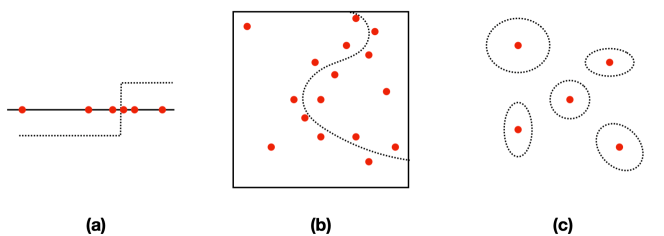
Figure 1: MaxiMin Active Learning strategically selects examples for labeling (red points). (a) reduces to binary search in simple 1-d threshold problem setting; (b) labeling is focused near decision boundary in multidimensional setting; (c) automatically discovers clusters and labels representative examples from each.

This paper builds on a new framework for active learning in the overparameterized and interpolationg regime, focusing on kernel methods and two-layer neural networks in the binary classification setting. The approach, called MaxiMin Active Learning, is based on mininum norm interpolating models. Roughly speaking, at each step of the learning process the maximin criterion requests a label for the example that is most difficult to interpolate. A minimum norm interpolating model is constructed for each possible example and the one yielding the largest norm indicates which example to label next. The rationale for the maximin criterion is that labeling the most challenging examples first may eliminate the need to label many of the other examples.

The maximin selection criterion is studied through experiments and mathematical analysis. We prove that the criterion has a number of desirable properties:

1. It tends to label examples near the current (estimated) decision boundary and close to oppositely labeled examples, allowing the active learning algorithm to focus on learning decision boundaries.

2. It reduces to optimal bisection in the one-dimensional linear classifier setting.

3. A data-based form of the criterion also provably discovers clusters and also automatically generates labeled coverings of the dataset.

Experimentally, we show that these properties generalize in several ways. For example, we find that in multiple dimensions the maximin criterion leads to a multidimensional bisection-like process that automatically finds a portion of the decision boundary and then locally explores to efficiently identify the complete boundary. We also show that MaxiMin Active Learning can learn hand-written digit classifiers with far fewer labeled examples than traditional passive learning based on labeling a randomly selected subset of examples.

2 A New Active Learning Criterion

At each iteration of the active learning algorithm, looking at the currently labeled set of samples, a new unlabeled point is selected to be labeled. The criterion we are proposing to pick the samples to be labeled is based on a ‘maximin’ operator. We will describe the criterion in its most general form along with the intuition behind this choice of criterion. In the remainder of the paper, we will go through some theoretical results about the properties of variations of this criterion in various setups along with some additional descriptive numerical evaluations and simulations.

2.1 Nonparametric Pool-based Active Learning

At each time step, the algorithm has access to a pool of labeled samples and a set of unlabaled samples. In other words, we have a partially labeled training set. Let $\mathcal{L}=\{(x_{1},y_{1}),\cdots,(x_{L},y_{L})\}$ be the set of labeled examples so far. We assume $x_{i}\in\mathcal{X}$ where $\mathcal{X}$ is the input/feature space and binary valued labels $y_{i}\in\{-1,+1\}$. Let $\mathcal{U}\subseteq\mathcal{X}$ be the set of unlabeled samples.

In the interpolating regime, the goal is to correctly label all the points in $\mathcal{U}$ so that the training error is zero. Passive learning generally requires labeling every point in $\mathcal{U}$. Active learning sequentially selects points in $\mathcal{U}$ for labeling with the aim of learning a correct classifier without necessarily labeling all of $\mathcal{U}$. Our setting can be viewed as an instance of pool-based active learning.

At each iteration, one unlabeled sample, $u^{*}\in\mathcal{U}$ is selected, labeled and added to the pool of labeled samples. The selection process is designed to pick the samples which are most informative upon being labeled. The proposed notion of score is the measure of informativeness of each sample $u\in\mathcal{U}$ at each time: the score of each unlabaled sample is computed, and the sample with the largest score is selected to be labeled.

$$u^{*}=\mathrm{argmax}_{u\in\mathcal{U}}\mathsf{score}(u)\,.$$ (1)

If there are multiple maximizers, then one is selected uniformly at random. Note that for any unlabeled sample $u\in\mathcal{U}$, the value of $\mathsf{score}(u)$ depends implicitly on the set of currently labeled points, $\mathcal{L}$. That is, information gained by labeling $u$ depends on the current knowledge of the learner. To define our proposed notion of $\mathsf{score}$, we define minimum norm interpolating function and introduce some notations next.

2.2 Minimum norm interpolating function

Let $\mathcal{F}$ be a class of functions mapping $\mathcal{X}$ to $\mathbb{R}$, where $\mathcal{X}$ is the input/feature space,. We assume the class $\mathcal{F}$ is rich enough to interpolate the training data. For example, $\mathcal{F}$ could be a nonparametric infinite dimensional Reproducing Kernel Hilbert Space (RKHS) or an overparameterized neural network representation.

Given the set of labeled samples, $\mathcal{L}$, and a class of functions $\mathcal{F}$, let $f\in\mathcal{F}$ be the interpolating function such that $f(x_{i})=y_{i}$ for all $(x_{i},y_{i})\in\mathcal{L}$. Note that there may be many functions that interpolate a discrete set of points such as $\mathcal{L}$. Among these, we choose $f$ to be the minimum norm interpolator:

$$f(x):= \,\mathrm{argmin}_{g\in\mathcal{F}}\,\,\|g\|_{\mathcal{F}}$$ (2)

s.t. $$\quad g(x_{i})=y_{i},\text{ for all }(x_{i},y_{i})\in\mathcal{L}\,.$$

Clearly, the definition of $f$ depends on the set of currently labeled samples $\mathcal{L}$ and the function norm $\|\cdot\|_{\mathcal{F}}$, although we omit these dependencies for ease of notation. The choice of $\mathcal{F}$ and the norm $\|\cdot\|_{\mathcal{F}}$ is application dependent. In this paper, we focus on (1) function classes represented by an overparameterized neural network representation with the $\ell^{2}$ norm of the weight vectors and (2) reproducing kernel Hilbert spaces with the corresponding Hilbert norm.

For unlabeled points $u\in\mathcal{U}$ and $\ell\in\{-1,+1\}$, define $f^{u}_{\ell}(x)$ is the minimum norm interpolating function based on current set of labeled samples $\mathcal{L}$ and the point $u\in\mathcal{U}$ with label $\ell$:

$$f^{u}_{\ell}(x):= \,\mathrm{argmin}_{g\in\mathcal{F}}\,\,\|g\|_{\mathcal{F}}$$ (3)

s.t. $$\quad g(x_{i})=y_{i},\text{ for all }(x_{i},y_{i})\in\mathcal{L}$$

$$\quad g(u)=\ell\,.$$

We use this definition in the next subsection to define the notion of $\mathsf{score}$.

2.3 Definition of proposed notion of $\mathsf{score}$

Roughly speaking, we want our selection criterion to prioritize labeling the most “informative” examples. Since the ultimate goal is to correctly label every example in $\mathcal{U}$, we design $\mathsf{score}(u)$ to measure the how hard it is to interpolate after adding $u$ to the set of labeled points. The intuition is that attacking the most challenging points in the input space first may eliminate the need to label other ‘easier’ examples later.

Note that we need to compute $\mathsf{score}(u)$ without knowing the label of $u$. To do so, we come up with an estimate of label of $u$, denoted by $\ell(u)\in\{-1,+1\}$ and compute $\mathsf{score}(u)$ assuming that upon labeling, $u$ will be labeled $\ell(u)$. We propose the following criterion for choosing $\ell(u)$:

$$\ell(u) :=\displaystyle{\mathrm{argmin}_{\ell\in\{-1,+1\}}}\|f_{\ell}^{u}(x)\|_{\mathcal{F}}\,.$$ (4)

Operating in the interpolating regime, we estimate the label of any unlabeled sample, $u$, to be the one that yields the minimum norm interpolant (i.e., the “smoother” of the two interpolants among the two possible functions $f_{+}^{u}(x)$ and $f_{-}^{u}(x)$).

Define

$$f^{u}(x):=f_{\ell(u)}^{u}(x)$$ (5)

to be the interpolating function after adding the sample $u$ with the label $\ell(u)$, defined in (4).

We propose two notions of $\mathsf{score}$. For $u\in\mathcal{U}$, define

$$\mathsf{score}_{\mathcal{F}}(u) = \|f^{u}(x)\|_{\mathcal{F}}\,$$ (6)

$$\mathsf{score}_{\mathtt{D}}(u) = \|f^{u}(x)-f(x)\|_{\mathtt{D}}\,$$ (7)

where $\|\cdot\|_{\mathcal{F}}$ is the norm associated the the function space $\mathcal{F}$. The function $f$ is the minimum norm interpolator of the labeled examples in $\mathcal{L}$ (defined in (2)), and $f^{u}(x)$ is defined (5) as the minimum norm interpolator after adding $u$ with the estimated label $\ell(u)$ to the set of labeled points. Also, define

$$\|g\|_{\mathtt{D}}\ =\ \int_{\mathcal{X}}|g(x)|^{2}\,\mbox{d}P_{X}(x)\ ,$$ (8)

where $P_{X}$ is the distribution of $x$. In practice, $P_{X}$ is the empirical distribution of $\mathcal{U}$. We refer to the (6) as the function norm score and (7) as the data-based norm score.

The distinction between the two definitions of the $\mathsf{score}$ function is as follows. Scoring unlabeled points according to the definition $\mathsf{score}_{\mathcal{F}}$ priotorizes labeling the examples which result in minimum norm interpolating functions with largest norm. Since the norm of the function can be associated with its smoothness, roughly speaking, this means that this criterion picks the points which give the least smooth interpolating functions. However, $\mathsf{score}_{\mathcal{F}}$ is insensitive to the distribution of data. The data-based $\mathsf{score}_{\mathtt{D}}$, in contrast, is sensitive to the distribution of the data. Measuring the difference between the new interpolation $f^{u}$ and the previous one makes this also sensitive to the structure of the function class.

With these definitions in place, we state the MaxiMin Active Learning criterion as follows. Given labeled data $\mathcal{L}$, the next example $u^{*}\in\mathcal{U}$ to label is selected according to

$$f^{u} = \arg\min_{f\in\{f_{+}^{u},f_{-}^{u}\}}\|f\|_{\mathcal{F}}\ ,\ \forall u\in\mathcal{U}$$

$$u^{*} = \arg\max_{u\in\mathcal{U}}\mathsf{score}(u)$$

with either $\mathsf{score}_{\mathcal{F}}$ or $\mathsf{score}_{\mathtt{D}}$.

3 MaxiMin Active Learning with Neural Networks

3.1 Overparameterized Neural Networks and Interpolation

Neural networks are often highly overparameterized and exactly fit to training data, yet remarkably the learned models generalize well to new data. A mathematical understanding of this phenomenom is beginning to emerge [1, 2, 3, 4, 5, 6, 7, 8]. This work suggests that among all the networks that could be fit to the training data, the learning algorithms used in training favor networks with smaller weights, providing a sort of implicit regularization. With this in mind, researchers have shown that even shallow networks and classical kernel methods fit to the data but regularized to have small weights (e.g., minimum norm fit to data) can generalize well [2, 9, 8, 10]. The functional mappings generated by wide, two-layer neural networks with Rectified Linear Unit (ReLU) activation functions were studied in [20]. It is shown that exactly fitting such networks to training data subject to minimizing the $\ell^{2}$-norm of the network weights results in a linear spline interpolation. This result was extended to a broad class of interpolating splines by appropriate choices of activation functions [21]. Our analysis of the MaxiMin active learning with neural networks will leverage these connections.

3.2 Neural Network Regularization

It has been long understood that the size of neural network weights, rather than simply the number of weights/neurons, characterizes the complexity of neural networks [22]. Here we focus on two-layer neural networks with ReLU activation functions in the hidden layer. If $\boldsymbol{x}\in{\mathbb{R}}^{d}$ is input to the network, then the output is computed by the function

$$f_{{\boldsymbol{w}},\boldsymbol{b},c}(\boldsymbol{x}) = \sum_{n=1}^{N}v_{n}\,\sigma(\boldsymbol{u}_{n}^{T}\boldsymbol{x}+b_{n})\ +\ c\ ,$$ (9)

where $\sigma(\cdot)=\max\{0,\cdot\}$ is the ReLU activation, ${\boldsymbol{w}}:=\{v_{n},\boldsymbol{u}_{n}\}_{n=1}^{N}$ are the “weights” of the network, and $\boldsymbol{b}:=\{b_{n}\}$ and $c$ are constant “bias” terms. The “norm” of $f_{{\boldsymbol{w}},\boldsymbol{b},c}$ is defined as $\|f_{{\boldsymbol{w}},\boldsymbol{b},c}\|:=\|{\boldsymbol{w}}\|_{2}$, the $\ell_{2}$-norm of the vector of network weights. We use the term norm in quotes because technically the weight norm does not correspond to a true norm on the function $f_{{\boldsymbol{w}},\boldsymbol{b},c}$ since, for example, constant functions $f_{{\boldsymbol{w}},\boldsymbol{b},c}=c$ have $\|{\boldsymbol{w}}\|_{2}=0$. From now on we will drop the subscripts and just write $f$ for ease of notation. Let $\{(x_{i},y_{i})\}_{i=1}^{M}$ be a set of training data. The minimum “norm” neural network interpolation of these data is the solution to the optimization

$$\min_{{\boldsymbol{w}}}\|{\boldsymbol{w}}\|_{2}\mbox{ subject to }f(x_{i})=y_{i},\ i=1,\dots,M.$$

A solution exists if the number of neurons $N$ is sufficiently large (see Theorem 5.1 in [23]).

In Section 5 we explore the behavior of MaxiMin active learning through numerical experiments using both the function “norm” score and the data-based norm score. In all our experiments and theory, we assume the binary classification setting where $y_{i}=\pm 1$. Broadly speaking, we observe the following behaviors.

1. With the function “norm” score the MaxiMin active learning algorithm tends to sample aggressively in the vicinity of the boundary, prefering to gather new labels between the closest oppositely labeled examples.

2. The data-based norm score is sensitive to the distribution of the data. It strikes a balance between exploiting regions between oppositely labeled examples (as in the function-based case) and exploring regions further away from labeled examples. Thus we see evidence that the data-based norm can effectively seek out the decision boundary and explore data clusters.

These behaviors are supported by a formal analysis of MaxiMin active learning in one dimension, discussed next.

3.3 MaxiMin Active Learning in One-Dimension

Our analysis of MaxiMin active learning with neural networks will focus on the behavior in one-dimension. We show that MaxiMin active learning with a two-layer ReLU netwok recovers optimal bisection learning strategies. The following characterization of minimum “norm” neural network interpolation in one-dimension follows from [20, 21] (see Theorem 4.4 and Proposition 6.1 in [21]).

Theorem 1.

Let $f:{\mathbb{R}}\rightarrow{\mathbb{R}}$ be a two-layer neural network with ReLU activation functions and $N$ hidden nodes as in (9). Let $\{(x_{i},y_{i})\}_{i=1}^{M}$ be a set of training data. If $N\geq M$, then a solution to the optimization

$$\min_{{\boldsymbol{w}}}\|{\boldsymbol{w}}\|_{2}\mbox{ subject to }f(x_{i})=y_{i},\ i=1,\dots,M$$

is a minimal knot linear spline interpolation of the points $\{(x_{i},y_{i})\}_{i=1}^{M}$.

In our analysis, we exploit the equivalence between minimum “norm” neural networks and linear splines. Specifically, a solution to the optimization is an interpolating function that is linear between each pair of neighboring points. This ensures that given a pair of neighboring labeled points $x_{1}$ and $x_{2}$ and any unlabeled point $x_{1}<u<x_{2}$, adding $u$ to the set of labeled points can only potentially change the interpolating function between $x_{1}$ and $x_{2}$. To eliminate uncertainty in the boundary conditions of the interpolation, we assume that the neural network is initialized by labeling the leftmost and rightmost points in the dataset and forced to have a constant extension to the left and right of these points (this can be accomplished by adding two artificial points to the left and right with the same labels as the true endpoints).

The main message of our analysis is that MaxiMin active learning with two-layer ReLU networks recovers optimal bisection (binary search) in one-dimension. This is summarized by the next corollary which follows in a straightforward fashion from Theorems 2 and 3.

Corollary 1.

Consider $N$ points uniformly distributed in the interval $[0,1]$ labeled according to a $k$-piecewise constant function $f$ so that $y_{i}=f(x_{i})\in\{-1,+1\}$, $i=1,\dots,N$, and length of the pieces are $\Theta(1/K)$. Then after labeling $O(k\log N)$ examples, the MaxiMin active learning with a two-layer ReLU network correctly labels all $N$ examples (i.e., the training error is zero).

The corollary follows from the fact that the MaxiMin criteria (both function norm and data-based norm) selects the next example to label at the midpoint between neighboring and oppositely labeled examples (i.e., at a bisection point). This is characterized in the next two theorems. First we consider the function “norm” criterion. The proof of the following theorem appears in Appendix A.1.

Theorem 2.

Let $\mathcal{L}$ be a set of labeled examples and let $u$ be an unlabeled example. Let $f_{+}^{u}$ be the minimum “norm” interpolator of $\mathcal{L}\cup(u,+1)$ and let $f_{-}^{u}$ be the minimum “norm” interpolator of $\mathcal{L}\cup(u,-1)$. Define the score of an unlabeled example $u$ as $\mathsf{score}_{\mathcal{F}}(u)\ =\ \min\{\|f_{+}^{u}\|,\|f_{-}^{u}\|\}$, where $\|f\|=\|{\boldsymbol{w}}\|_{2}$, the neural network weight norm. Then, the selection criterion based on $\mathsf{score}_{\mathcal{F}}$ has the following properties

1. Let $x_{1}$ and $x_{2}$ be two oppositely labeled neighboring points in $\mathcal{L}$, i.e., no other points between $x_{1}$ and $x_{2}$ have been labeled and $y_{1}\neq y_{2}$. Then for all $x_{1}<u<x_{2}$, $\mathsf{score}_{\mathcal{F}}\left(\frac{x_{1}+x_{2}}{2}\right)\geq\mathsf{score}_{\mathcal{F}}(u)$.

2. Let $x_{1}<x_{2}$ and $x_{3}<x_{4}$ be two pairs of oppositely labeled neighboring points (i.e., $y_{1}\neq y_{2}$ and $y_{3}\neq y_{4}$) such that $x_{2}-x_{1}\geq x_{4}-x_{3}$. Then,

   $$\mathsf{score}_{\mathcal{F}}\left(\frac{x_{1}+x_{2}}{2}\right)\ \leq\ \mathsf{score}_{\mathcal{F}}\left(\frac{x_{3}+x_{4}}{2}\right)\,.$$

3. Let $x_{5}$ and $x_{6}$ be two identically labeled neighboring points in $\mathcal{L}$, i.e., $y_{5}=y_{6}$. Then for all $x_{5}<u<x_{6}$, the function $\mathsf{score}_{\mathcal{F}}(u)$ is constant.

4. For any pair of neighboring oppositely labeled points $x_{1}$ and $x_{2}$, any pair of neighboring identically labeled points $x_{5}$ and $x_{6}$, any $x_{1}<u<x_{2}$ and any $x_{5}<v<x_{6}$, we have

   $$\mathsf{score}_{\mathcal{F}}(v)\leq\mathsf{score}_{\mathcal{F}}(u)\,.$$

Now we turn to the data-based norm. Here we observe the effect of the data distribution on the bisection properties. The properties mirror those in Theorem 2 except in the case of the second property. The data-based norm criterion tends to sample in the largest (most data-massive) interval between oppositely labeled points, whereas the function-based norm criterion favors points in the smallest interval.

Theorem 3.

Let the distribution $\mathbb{P}(X)$ be uniform over an interval. Let $\mathcal{L}$ be a set of labeled examples and let $u$ be an unlabeled example. Let $f_{+}^{u}$ be the minimum “norm” interpolator of $\mathcal{L}\cup(u,+1)$ and let $f_{-}^{u}$ be the minimum “norm” interpolator of $\mathcal{L}\cup(u,-1)$ and let $f^{u}=\arg_{g\in\{f_{+}^{u},f_{-}^{u}\}}\|g\|$ consistent with notations in (3) and (5). Then $\mathsf{score}_{\mathtt{D}}(u)=\int|f^{u}(x)-f(x)|^{2}\,dP_{X}(x)$, where $f$ is the minimum “norm” interpolator based on the labeled data $\mathcal{L}$. Then, the selection criterion based on $\mathsf{score}_{\mathtt{D}}$ has the following properties.

1. Let $x_{1}$ and $x_{2}$ be two oppositely labeled neighboring points in $\mathcal{L}$, i.e., $y_{1}\neq y_{2}$. Then for all $x_{1}<u<x_{2}$ $\mathsf{score}_{\mathtt{D}}\left(\frac{x_{1}+x_{2}}{2}\right)\geq\mathsf{score}_{\mathtt{D}}(u)$.

2. Let $x_{1}<x_{2}$ and $x_{3}<x_{4}$ be two pairs of oppositely labeled neighboring labeled points (i.e., $y_{1}\neq y_{2}$ and $y_{3}\neq y_{4}$) such that $x_{2}-x_{1}\geq x_{4}-x_{3}$. If the unlabeled points are uniformly distributed in each interval and the number of points is in $(x_{1},x_{2})$ is less than the number in $(x_{4},x_{3})$, then

   $$\mathsf{score}_{\mathtt{D}}\left(\frac{x_{1}+x_{2}}{2}\right)\geq\mathsf{score}_{\mathtt{D}}\left(\frac{x_{3}+x_{4}}{2}\right)\,.$$

3. Let $x_{5}$ and $x_{6}$ be two identically labeled neighboring points in $\mathcal{L}$, i.e., $y_{5}=y_{6}$. Then for all $x_{5}<v<x_{6}$, we have $\mathsf{score}_{\mathtt{D}}(v)=0$.

4. For any pair of neighboring oppositely labeled points $x_{1}$ and $x_{2}$, any pair of neighboring identically labeled points $x_{5}$ and $x_{6}$, any $x_{1}<u<x_{2}$ and any $x_{5}<v<x_{6}$, we have

   $$\mathsf{score}_{\mathtt{D}}(v)\leq\mathsf{score}_{\mathtt{D}}(u)\,.$$

The proof appears in Appendix A.2.

4 Interpolating Active Learners in an RKHS

In this section, we will focus on minimum norm interpolating functions in a Reproducing Kernel Hilbert Space (RKHS). We present theoretical properties for general RKHS settings, detailed analytical results in the one-dimensional setting, and numerical studies in multiple dimensions. Broadly speaking, we establish the following properties: the proposed score functions

$\bullet$ tend to select examples near the decision boundary of $f$, the current interpolator;

$\bullet$ the score is largest for unlabeled examples near the decision boundary and close to oppositely labeled examples, in effect searching for the boundary in the most likely region of the input space;

$\bullet$ in one dimension the interpolating active learner coincides with an optimal binary search procedure;

$\bullet$ using data-based function norms, rather than the RKHS norm, the interpolating active learner executes a tradeoff between sampling near the current decision boundary and sampling in regions far away from currently labeled examples, thus exploiting cluster structure in the data.

4.1 Kernel Methods

A Hilbert space $\mathcal{H}$ is associated with an inner product: $\langle f,g\rangle_{\mathcal{H}}$ for $f,g\in\mathcal{H}$. This induces a norm defined by $\|f\|_{\mathcal{H}}=\sqrt{\langle f,f\rangle}_{\mathcal{H}}$. A symmetric bivariate function $K:\mathcal{X}\times\mathcal{X}\to\mathbb{R}$ is positive semidefinite if for all $n\geq 1$, and points $\{x_{i}\}_{i=1}^{n}$, the matrix K with element $\textbf{K}_{i,j}=K(x_{i},x_{j})$ is positive semidefinite (PSD). These functions are called PSD kernel functions. A PSD kernel constructs a Hilbert space, $\mathcal{H}$ of functions on $f:\mathcal{X}\to\mathbb{R}$. For any $x\in\mathcal{X}$ and any $f\in\mathcal{H}$, the function $K(\cdot,x)\in\mathcal{H}$ and $\langle f,K(\cdot,x)\rangle_{\mathcal{H}}=f(x)$. Throughout this section, we assume $K(x,x)=1$.

For the set of labeled samples $\mathcal{L}=\{(x_{1},y_{1}),\cdots,(x_{L},y_{L})\}$ with $y_{i}\in\{-1,+1\}$, let the function $f(x)$ be decomposed as

$$f(x) =\sum_{i=1}^{L}\alpha_{i}k(x_{i},x)$$ (10)

$$\text{with}\quad\alpha =\textbf{K}^{-1}\textbf{y},$$

where $\textbf{K}=\big{[}\textbf{K}_{i,j}\big{]}_{i,j}$ is the $L$ by $L$ matrix such that $\textbf{K}_{i,j}=k(x_{i},x_{j})$ and $\textbf{y}=[y_{1},\cdots,y_{L}]^{T}$. Using reproducible kernels implies that $f(x)\in\mathcal{H}$ for the a RKHS $\mathcal{H}$. Then, $f(x)$ defined above is the minimum Hilbert norm interpolating function defined in (2). Using the property $\langle K(x_{i},\cdot),K(x_{j},\cdot)\rangle=K(x_{i},x_{j})$, we have

$$\|f(x)\|_{\mathcal{H}}^{2}=\alpha^{T}\,\textbf{K}\,\alpha=\textbf{y}^{T}\,\textbf{K}^{-1}\,\textbf{y}\,.$$

For $u\in\mathcal{U}$ and ${\ell}\in\{-1,+1\}$, the minimum norm interpolating unction $f^{u}_{\ell}(x)$, defined in (3) (based on currently labeled samples $\mathcal{L}$ and sample $u$ with label ${\ell}$) is derived similarly :

$$f^{u}_{\ell}(x) =\sum_{i=1}^{L}\widetilde{\alpha}_{i}k(x_{i},x)+\widetilde{\alpha}_{L+1}k(u,x)$$ (11)

$$\text{with}\quad\widetilde{\alpha} =\widetilde{\textbf{K}}_{u}^{-1}\widetilde{\textbf{y}}_{\ell},$$

where

$$\widetilde{\textbf{K}}_{u}=\begin{bmatrix}\textbf{K}&\textbf{a}_{u}\\ \textbf{a}_{u}^{T}&b\end{bmatrix}\,,\,\,\textbf{a}_{u}=\begin{bmatrix}k(x_{1},u)\\ \vdots\\ k(x_{L},u)\end{bmatrix}\,,\,\,\widetilde{\textbf{y}}_{\ell}=\begin{bmatrix}\textbf{y}\\ {\ell}\end{bmatrix}\,,\,\,\text{and}\,\,b=K(u,u)\,.$$ (12)

Throughout this paper, we use kernel such that $K(x,x)=1$ for all $x\in\mathcal{X}$.

4.2 Properties of General Kernels for Active Learning

We first show that using kernel based function spaces for interpolation, ${\ell}(u)$ defined in (4) coincides with the sign of value of current interpolator at $u$.

Proposition 1.

For $u\in\mathcal{X}$ and ${\ell}\in\{-,+\}$, define $f(x)$ and $f_{\ell}^{u}(x)$ according to (2) and (3) in Section 2. Then, $\ell(u)$ defined in (4) satisfies

$${\ell}(u)=\begin{cases}+1\quad\quad\text{ if }f(u)\geq 0\\ -1\quad\quad\text{ if }f(u)<0\,.\end{cases}$$

Proof.

Let $\widetilde{\textbf{y}}_{\ell}=[y_{1},\cdots,y_{n},{\ell}]^{T}$, $\textbf{a}_{u}=[K(x_{1},u),\cdots,K(x_{n},u)]^{T}$ and $b=K(u,u)=1$. Let K be the kernel matrix for the elements in $\mathcal{L}$ and $\widetilde{\textbf{K}}_{u}$ be the kernel matrix for the elements in $\mathcal{L}\cup\{u\}$, as defined in (12). Then, for ${\ell}\in\{-1,+1\}$

$$\|f^{u}_{\ell}(x)\|_{\mathcal{H}}^{2} =\widetilde{\textbf{y}}_{\ell}^{T}\,\,\widetilde{\textbf{K}}_{u}^{-1}\,\,\widetilde{\textbf{y}}_{\ell}\overset{(a)}{=}\textbf{y}^{T}\,\,\Big{(}\textbf{K}-\textbf{a}_{u}\,\textbf{a}_{u}^{T}\Big{)}^{-1}\,\,\textbf{y}-2{\ell}\,\,\textbf{y}^{T}\,\Big{(}\textbf{K}-\textbf{a}_{u}\,\textbf{a}_{u}^{T}\Big{)}^{-1}\textbf{a}+\Big{(}1-\textbf{a}_{u}^{T}\,\textbf{K}^{-1}\textbf{a}_{u}\Big{)}^{-1}$$

$$\overset{(b)}{=}\textbf{y}^{T}\,\,\textbf{K}^{-1}\,\,\textbf{y}+\frac{\Big{(}1-{\ell}\,\textbf{y}^{T}\,\,\textbf{K}^{-1}\textbf{a}_{u}\Big{)}^{2}}{1-\textbf{a}_{u}^{T}\,\textbf{K}^{-1}\textbf{a}_{u}}\overset{(c)}{=}\|f(x)\|_{\mathcal{H}}^{2}+\frac{\big{[}1-{\ell}\,f(u)\big{]}^{2}}{1-\textbf{a}_{u}^{T}\,\textbf{K}^{-1}\textbf{a}_{u}}\,.$$

where Schur’s complement formula gives (a) and Woodbury Identity with some algebra algebra gives (b). We are using the property that $K(x,x)=1$ and the diagonal elements of matrix $\widetilde{\textbf{K}}_{u}$ are equal to one. (c) uses (10) for the minimum norm interpolating function based on $\mathcal{L}$, i.e., $f(x)$. Hence, $\|f^{u}_{+}(x)\|_{\mathcal{H}}>\|f^{u}_{-}(x)\|_{\mathcal{H}}$ if and only if $f(u)<0$ which gives the statement of proposition. ∎

4.3 Radial Basis Kernels

From here on, we will focus on minimum norm interpolating functions with radial basis kernels. The kernel functions we use have the following form: For $x,x^{\prime}\in\mathbb{R}^{d}$, $h>0$ and $p>1$, let

$$k_{h,p}(x,x^{\prime})=\exp\Big{(}-\frac{1}{h}\|x-x^{\prime}\|_{p}\Big{)}\,,$$ (13)

where $\|x\|_{p}:=\big{(}\sum_{i=1}^{d}x_{i}^{p}\big{)}^{1/p}$ is the $\ell_{p}$ norm and $\|x-x^{\prime}\|_{p}$ is the Minkowski distance satisfying the triangle inequality. For $p=1,2$ this category of kernels construct Reproducing Kernel Hilbert Spaces. When the parameters $h$ and $p$ are specified, we denote the kernel function $k_{h,p}(x,y)$ by $k(x,y)$.

4.4 Laplace Kernel in One Dimension

To develop some intuition, we consider active learning in one-dimension. The sort of target function we have in mind is a multiple threshold classifier. Optimal active learning in this setting coincides with binary search. We now show that the proposed selection criterion based on $\mathsf{score}_{\mathcal{H}}$ with Hilbert norm associated with the Laplace kernels result in an optimal active learning in one dimension (proof in Appendix B.1).

Proposition 2.

[Maximin criteria in one dimension with Laplace kernel] Define $K(x,x^{\prime})=\exp(-|x-x^{\prime}|/h)$ to be the Laplace kernel in one dimension and the minimum norm interpolator function defined in Section 4.1. Let the selection criterion be based on $\mathsf{score}_{\mathcal{H}}(u)$ function defined in (6) with the Laplace kernel Hilbert norm. Then the following statements hold for any value of $h>0$:

1. Let $x_{1}$ and $x_{2}$ be two neighboring labeled points in $\mathcal{L}$. Then $\mathsf{score}_{\mathcal{H}}\left(\frac{x_{1}+x_{2}}{2}\right)\geq\mathsf{score}_{\mathcal{H}}(u)$ for all $x_{1}<u<x_{2}$.

2. Let $x_{1}<x_{2}$ and $x_{3}<x_{4}$ be two pairs of neighboring labeled points such that $x_{2}-x_{1}\geq x_{4}-x_{3}$, then

   • if $y_{1}\neq y_{2}$ and $y_{3}=y_{4}$. Then $\mathsf{score}_{\mathcal{H}}\left(\frac{x_{1}+x_{2}}{2}\right)\geq\mathsf{score}_{\mathcal{H}}\left(\frac{x_{3}+x_{4}}{2}\right)$.

   • if $y_{1}=y_{2}$ and $y_{3}\neq y_{4}$. Then $\mathsf{score}_{\mathcal{H}}\left(\frac{x_{1}+x_{2}}{2}\right)\leq\mathsf{score}_{\mathcal{H}}\left(\frac{x_{3}+x_{4}}{2}\right)$.

   • if $y_{1}\neq y_{2}$ and $y_{3}\neq y_{4}$. Then $\mathsf{score}_{\mathcal{H}}\left(\frac{x_{1}+x_{2}}{2}\right)\leq\mathsf{score}_{\mathcal{H}}\left(\frac{x_{3}+x_{4}}{2}\right)$.

   • if $y_{1}=y_{2}$ and $y_{3}=y_{4}$. Then $\mathsf{score}_{\mathcal{H}}\left(\frac{x_{1}+x_{2}}{2}\right)\geq\mathsf{score}_{\mathcal{H}}\left(\frac{x_{3}+x_{4}}{2}\right)$.

The key conclusion drawn from these properties is that the midpoints between the closest oppositely labeled neighboring examples have the highest score. If there are no oppositely labeled neighbors, then the score is largest at the midpoint of the largest gap between consecutive samples. Thus, the score results in a binary search for the thresholds definining the classifier. Using the proposition above, it is easy to show the following result, proved in the Appendix B.3.

Corollary 2.

Consider $N$ points uniformly distributed in the interval $[0,1]$ labeled according to a $k$-piecewise constant function $g(x)$ so that $y_{i}=g(x_{i})\in\{-1,+1\}$ and length of the pieces are roughly on the order of $\Theta(1/K)$. Then by running the proposed active learning algorithm with Laplace Kernel and any bandwidth, after $O(k\log N)$ queries the sign of the resulting interpolant $f$ correctly labels all $N$ examples (i.e., the training error is zero).

This statement is true for $N>5/h$. The proof is provided in Appendix B.3.

4.5 General Radial-Basis Kernels in One Dimension

In the next proposition, we look at the special case of radial basis kernels, defined in Equation(13) applied to one dimensional functions with only three initial points. We show how maximizing $\mathsf{score}_{\mathcal{H}}$ with the appropriate Hilbert norm is equivalent to picking the zero-crossing point of our current interpolator.

Proposition 3 (One Dimensional Functions with Radial Basis Kernels).

Assume that for any pair of samples $x,x^{\prime}\in\mathcal{L}$ we have $|x-x^{\prime}|\geq\Delta$. Assume $\Delta h^{-1/p}\geq D$ for a constant value of $D$. Let $x_{1}<x_{2}<x_{3}\in\mathbb{R}$, $y_{1}=y_{2}=+1$ and $y_{3}=-1$. For $u$ such that $x_{2}+\Delta/2<u<x_{3}-\Delta/2$, we have $\mathsf{score}_{\mathcal{H}}(u)\leq\mathsf{score}_{\mathcal{H}}(u^{*})$ where $u^{*}$ is the point satisfying $f(u^{*})=0$.

The proof is rather tedious and appears in Appendix C.1. But the idea is based on showing that with small enough bandwidth, $\|f^{u}_{+}\|$ is increasing in $u$ in the interval $[x_{2}+\Delta/2,x_{3}-\Delta/2]$ and $\|f^{u}_{-}\|$ is decreasing in $u$ in the same interval. This shows that $\max_{u}\min_{\ell\in\{-1,+1\}}\|f^{u}_{\ell}\|$ occurs at $u^{*}$ such that $\|f^{u^{*}}_{+}\|=\|f^{u^{*}}_{-}\|$. We showed that this is equivalent to the condition $f(u^{*})=0$.

4.6 Properties of data based-norm criterion

Intuitively, $\mathsf{score}_{\mathtt{D}}$ measures the expected change in the squared norm over all unlabeled examples if $u\in{\cal U}$ is selected as the next point. This norm is sensitive to the particular distribution of the data, which is important if the data are clustered. This behavior will be demonstrated in the multidimensional setting discussed next.

In this section, we present two theoretical results on the properties of data-based norm selection criterion. To do so, we will prove the properties of the selected examples based on the data-based norm in the context of the clustered data. In particular, if the support of the generative distribution $P_{X}(x)$ is composed of several disjoint clusters, the data-based norm criterion prioritizes labeling samples from bigger clusters first. Subsequently, it selects a sample from each cluster to be labeled. If the clustering in the dataset is aligned with their labels (most of the samples in the same cluster are in the same class), labeling one sample in each cluster ensures rapid decay in the probability of error of the classifier as a function of number of labeled samples. This behavior is consistent with numerical simulations presented in Section 5.

The next theorem will show that if the clusters are well-separated (the distance between the clusters are sufficiently large), then the first example to be selected to for labeling is in the biggest cluster.

Theorem 4 (First point in clustered data).

Fix $p>1$ and $h>0$. Let the distribution $\mathbb{P}(X)$ be uniform over $M$ disjoint sets $B_{1},\cdots,B_{M}$ such that $B_{i}$ is an $\ell_{p}$ ball with radius $r_{i}$ and center $c_{i}$, i.e.,

$$B_{i}=\mathcal{B}_{d,p}(r_{i};c_{i}):=\{x\in\mathbb{R}^{d}:\|x-c_{i}\|_{p}\leq r_{i}\}\,.$$ (14)

Without loss of generality, assume $r_{1}>r_{2}>\cdots>r_{K}$. Define $D=\min_{i\neq j}\|c_{i}-c_{j}\|_{p}-2r_{1}$ as an upper bound for the minimum distance between the clusters.

Assume $\mathcal{L}=\varnothing$ and let the interpolating functions $f$ be defined in (10) with $k_{h,p}$ (defined in (13)). The selection criterion is based on the $\mathsf{score}_{\mathtt{D}}$ function defined in (7). If

$$D>\frac{h}{2}\Big{[}\ln M-\ln\big{(}1-(r_{2}/r_{1})^{d}\big{)}\Big{]}\quad\quad\text{and}\quad\quad r_{1}\leq h/2,$$

then the first point to be labeled is in the biggest ball, $B_{1}$.

The proof is presented in Appendix C.1.

The next theorem shows that if the distance between the clusters are sufficiently large and the radius of the clusters are not too large, then the active learning algorithm based on the notion of $\mathsf{score}$ with data-based norm labels one sample from each cluster before zooming in inside the clusters.

Theorem 5 (Cluster exploration).

Let $\mathcal{S}$ be the support of $P_{X}$. Assume $\mathcal{S}=\cup_{i=1}^{M}B_{i}$ where $B_{i}$’s are $\ell_{p}$-balls with radii $r$ and centers $c_{i}$. Define $D:=\min_{i\neq j}\|c_{i}-c_{j}\|_{p}-2r_{1}$ to be the minimum distance between the clusters. Let $\mathcal{L}=\{x_{1},x_{2},\cdots,x_{L}\}$ be $L<M$ labeled points such that $x_{1}\in B_{1},x_{2}\in B_{2},\cdots,x_{L}\in B_{L}$. Let the selection criterion be based on the $\mathsf{score}_{\mathtt{D}}$ function defined in (7). If $r<h/3$ and $D\geq 12h\ln(2M)$, then the next point to be labeled is in a new ball ($\cup_{i={L+1}}^{M}B_{i}$) containing no labeled points.

As a corollary of the above theorem, one can see that if the ratio of the distance between the clusters to the radius of clusters is sufficiently large ($D/r>36ln(2M)$), then one can use a kernel with proper bandwidth which picks one sample from each cluster initially. The proof is presented in Appendix C.2.

5 Numerical Simulations of kernel based

In this Section, we present the outcome of numerical simulations of the proposed selection criteria on synthetic and real data. In this section, $\mathsf{score}_{\mathcal{H}}$ is used to denoted the $\mathsf{score}$ function defined in (6) with the Hilbert norm associated with the Laplace Kernel. Similarly, $\mathsf{score}_{\mathtt{D}}$ is the $\mathsf{score}$ function defined in (7) with the data-based norm.

5.1 Bisection in one dimension

The bisection process is illustrated experimentally in the Figure 2 below. $\mathsf{score}_{\mathcal{H}}$ uses the RKHS norm. For comparison, we also show the behavior of the algorithm using $\mathsf{score}_{\mathtt{D}}$ and the data-based norm. Data selection using either score drives the error to zero faster than random sampling (as shown on the left). We clearly see the bisection behavior of $\mathsf{score}_{\mathcal{H}}$, locating one decision boundary/threshold and then another, as the proof corollary above suggests. Also, we see that the data-based norm does more exploration away from the decision boundaries. As a result, the data-based norm has a faster and more graceful error decay, as shown on the right of the figure. Similar behavior is observed in the multidimensional setting shown in Figure 5.

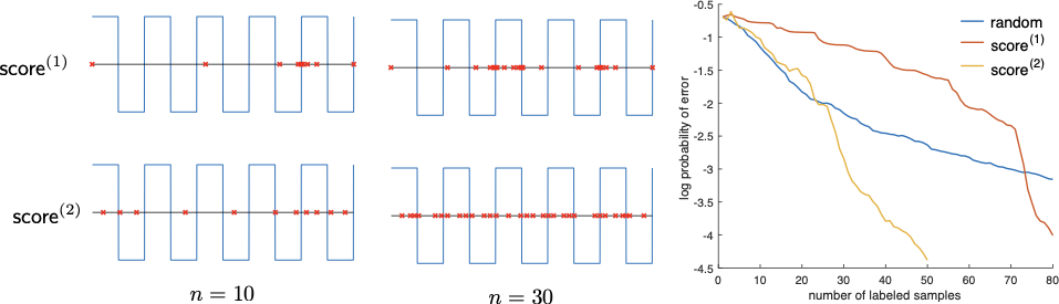
Figure 2: Uniform distribution of samples in unit interval, multiple thresholds between $\pm 1$ labels, and active learning using Laplace Kernel, Bandwidth$=.1$. Probability of error of the interpolated function shown on right.

5.2 Multidimensional setting with smooth boundary

The properties and behavior found in the one dimensional setting carry over to higher dimensions. In particular, the max-min norm criterion tends to select unlabeled examples near the decision boundary and close to oppositely labeled examples, This is illustrated in Figure 3 below. The inputs points (training examples) are uniformly distributed in the square $[-1,1]\times[-1,1]$. We trained an Laplace kernel machine to perfectly interpolate four training points with locations and binary labels as depicted in Figure 3(a). The color depicts the magnitude of the learned interpolating function: dark blue is $0$ indicating the “decision boundary” and bright yellow is approximately $3.5$. Figure 3(b) denotes the score for selecting a point at each location based on RKHS norm criterion. Figure 3(c) denotes the score for selecting a point at each location based on data-based norm criterion discussed above. Both criteria select the point on the decision boundary, but the RKHS norm favors points that are closest to oppositely labeled examples whereas the data-based norm favors points on the boundary further from labeled examples.

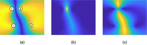
Figure 3: Data selection of Laplace kernel active learner. (a) Magnitude of output map kernel machine trained to interpolate four data points as indicated (dark blue is $0$ indicating the learned decision boundary). (b) Max-Min RKHS norm selection of next point to label. Brightest yellow is location of highest score and selected example. (c) Max-Min selection of next point to label using data-based norm. Both select the point on the decision boundary, but the RKHS norm favors points that are closest to oppositely labeled examples.

Next we present a modified scenario in which the examples are not uniformly distributed over the input space, but instead concentrated only in certain regions indicated by the magenta highlights in Figure 4(a). In this setting, the example selection criteria differ more significantly for the two norms. The weight norm selection criterion remains unchanged, but is applied only to regions where there are examples. Areas with out examples to select are indicated by dark blue in Figure 4(b)-(c). The data-based norm is sensitive to the non-uniform input distribution, and it scores examples near the lower portion of the decision boundary highest.

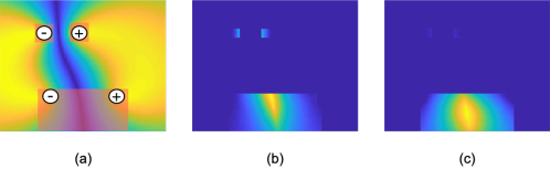
Figure 4: Data selection of Laplace kernel active learner. (a) Unlabeled examples are only available in magenta shaded regions. (b) Max-Min selection map using RKHS norm (6). (c) Max-Min selection map using data-based norm defined in Equation (7).

The distinction between the max-min selection criterion using the RKHS vs. data-based norm is also apparent in the experiment in which a curved decision boundary in two dimensions is actively learned using a Laplace kernel machine, as depicted in Figure 5 below. $\mathsf{score}_{\mathcal{H}}$ is the max-min RKHS norm criterion at progressive stages of the learning process (from left to right). The data-based norm is used in $\mathsf{score}_{\mathtt{D}}$ defined in Equation (7). Both dramatically outperform a passive (random sampling) scheme and both demonstrate how active learning automatically focuses sampling near the decision boundary between the oppositely labeled data (yellow vs. blue). However, the data-based norm does more exploration away from the decision boundary. As a result, the data-based norm requires slightly more labels to perfectly predict all unlabeled examples, but has a more graceful error decay, as shown on the right of the figure.

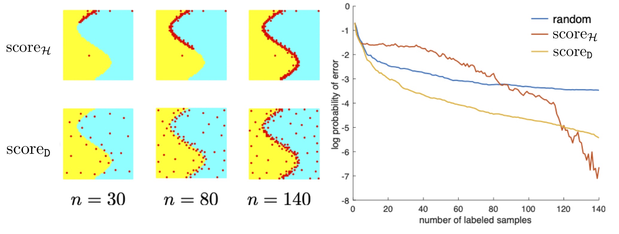
Figure 5: Uniform distribution of samples, smooth boundary, Laplace Kernel, Bandwidth$=.1$. On left, sampling behavior of $\mathsf{score}_{\mathcal{H}}$ and $\mathsf{score}_{\mathtt{D}}$ at progressive stages (left to right). On right, error probabilities as a function of number of labeled examples.

5.3 Multidimensional setting with clustered data

To capture the properties of the proposed selection criteria in clustered data, we implemented the algorithm on synthetic clustered data in Figures 6 and 7. We demonstrate how the data-based norm also tends to automatically select representive examples from clusters when such structure exists in the unlabeled dataset. Figure 6 compares the behavior of selection based on $\mathsf{score}_{\mathcal{H}}In$ with the RKHS norm and $\mathsf{score}_{\mathtt{D}}$ with data-based norm, when data are clusters and each cluster is homogeneously labeled. We see that the data-based norm quickly identifies the clusters and labels a representative from each, leading to faster error decay as shown on the right.

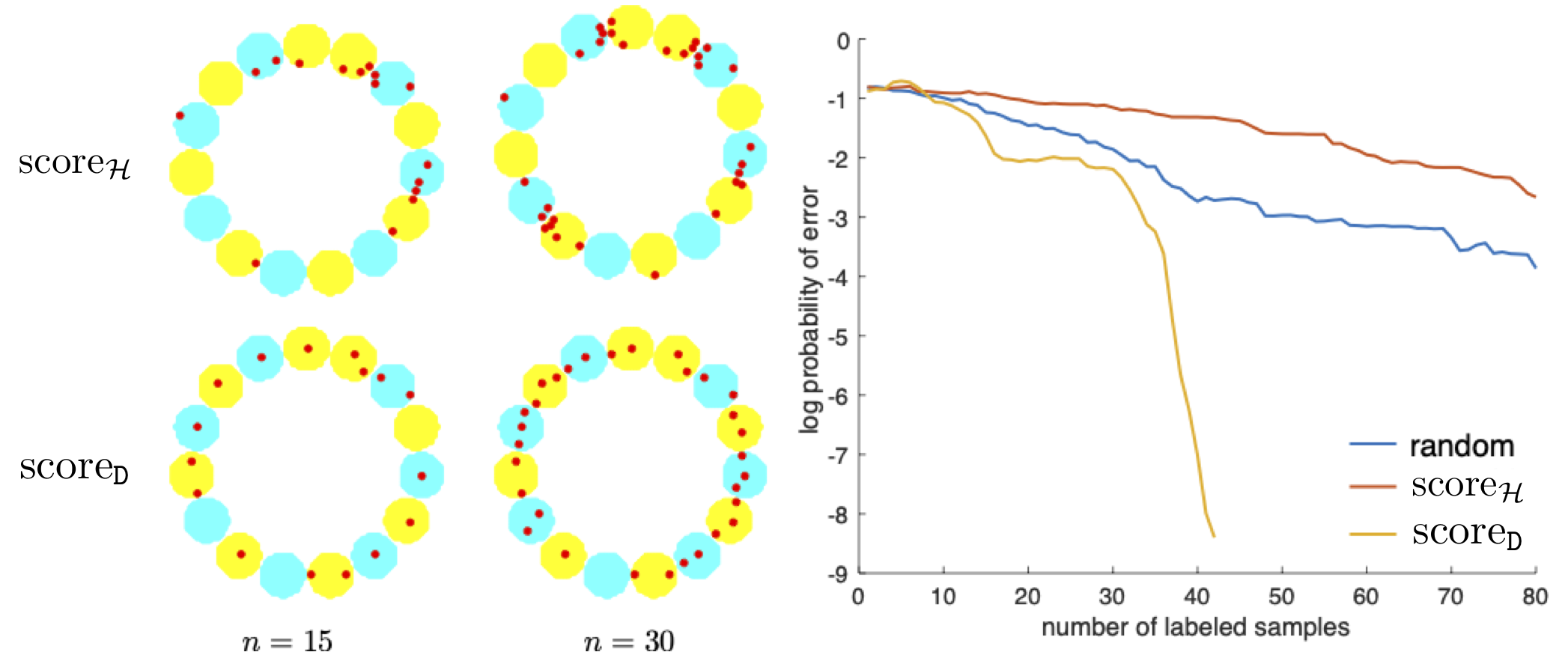
Figure 6: Uniform distribution of samples, smooth boundary, Laplace Kernel, Bandwidth$=.1$. On left, sampling behavior of $\mathsf{score}_{\mathcal{H}}$ and $\mathsf{score}_{\mathtt{D}}$ at progressive stages (left to right). On right, error probabilities as a function of number of labeled examples.

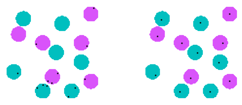
Figure 7: Points in blue and yellow clusters are labeled $+1$ and $-1$, respectively. The left figure uses $\mathsf{score}_{\mathcal{H}}$ to be the $\mathsf{score}$ function defined in (6) with the Hilbert norm associated with the Laplace Kernel. Similarly, $\mathsf{score}_{\mathtt{D}}$ is the $\mathsf{score}$ function defined in (7) with the data-based norm. The first 13 samples selected by $\mathsf{score}_{\mathcal{H}}$ and $\mathsf{score}_{\mathtt{D}}$ are depicted as black dots. $\mathsf{score}_{\mathtt{D}}$ has labeled one sample from each cluster, but $\mathsf{score}_{\mathcal{H}}$ has not labeled any samples from 5 clusters. Note that $\mathsf{score}_{\mathcal{H}}$ has spent some of the sample budget to discriminate between nearby clusters with opposite labels.

In the setup in Figure 7, the samples are generated based on a uniform distribution on 13 clusters. Points in blue and yellow clusters are labeled $+1$ and $-1$, respectively. We run the two variations of proposed active learning algorithms and compare their sampling strategy in this setup. The left figure uses $\mathsf{score}_{\mathcal{H}}$ to be the $\mathsf{score}$ function defined in (6) with the Hilbert norm associated with the Laplace Kernel. Similarly, $\mathsf{score}_{\mathtt{D}}$ is the $\mathsf{score}$ function defined in (7) with the data-based norm.

The selection criterion based on $\mathsf{score}_{\mathcal{H}}$ prioritizes sampling on the decision boundary of the current classifier where the currently oppositely labeled samples are close to each other. This behavior of the algorithm based on $\mathsf{score}_{\mathcal{H}}$ in one dimension is proved in Sections 4.4 and 4.5. Alternatively, $\mathsf{score}_{\mathtt{D}}$ prioritizes labeling at least one sample from each cluster. Hence, after labeling 13 samples, the active learning algorithm based on $\mathsf{score}_{\mathtt{D}}$ has one sample in each cluster, but the active learning algorithm based on $\mathsf{score}_{\mathtt{D}}$ has not labeled any samples in 5 clusters.

5.4 MNIST experiments

Here we illustrate the performance of the proposed active learning method on the MNIST dataset. We ran algorithms based on our proposed selection criteria for a binary classification task on MNIST dataset. The binary classification task used in this experiment assigns a label $-1$ to any digit in set $\{0,1,2,3,4\}$ and label $+1$ to $\{5,6,7,8,9\}$. The goal of the classifier is detecting whether an image belongs to the set of numbers greater or equal to $5$ or not. We used Laplace kernel as defined in (13) with $p=2$ and $h=10$ on the vectorized version of a dataset of $1000$ images. In Figures 8, $\mathsf{score}_{\mathcal{H}}$ is the $\mathsf{score}$ function defined in (6) with the Hilbert norm associated with the Laplace Kernel. Similarly, $\mathsf{score}_{\mathtt{D}}$ is the $\mathsf{score}$ function defined in (7) with the data-based norm.

To asses the quality of performance of each of the selection criteria, we compare the probability of error of the interpolator at each iteration. In particular, we plot the probability of error of the interpolator as a function of number of labeled samples, using the $\mathsf{score}_{\mathcal{H}}$ and $\mathsf{score}_{\mathtt{D}}$ functions on the training set and test set separately. For comparison, we also plot the probability of error when the selection criterion for picking samples to be labeled is random.

Figure 8 (a) shows the decay of probability of error in the training set. When the number of labeled samples is equal to the number of samples in the training set, it means that all the samples in training set are labeled and used in constructing the interpolator. Hence, the probability of error on the training set for any selection criterion is zero when number of labeled samples is equal to the number of samples in the training set. Figure 8 (b) shows the probability of error on the test set as a function of the number of labeled samples in the training set selected by each selection criterion.

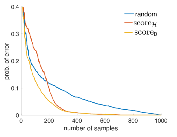
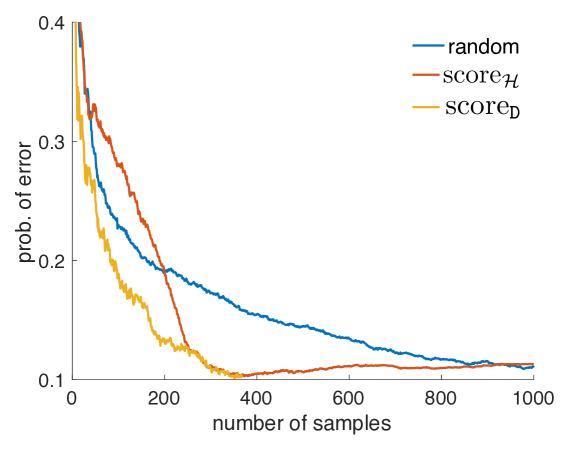
Figure 8: Probability of error for learning a classification task on MNIST data set. The performance of three selection criteria for labeling the samples: random selection, active selection based on $\mathsf{score}_{\mathcal{H}}$, and active selection based on $\mathsf{score}_{\mathtt{D}}$. The first curve depicts the probability of error on the training set and the second curve is the probability of error on the test set.

5.4.1 Clustering in MNIST

The binary classification task used in the MNIST experiment assigns a label $-1$ to any digit in set $\{0,1,2,3,4\}$ and label $+1$ to $\{5,6,7,8,9\}$. We expect that the images are clustered where each cluster would correspond to the images of a digit. We expect that the advantageous behavior of using data-based norm criterion in clustered data is one of the reasons for faster decay of probability of error of the $\mathsf{score}_{\mathtt{D}}$ in Figure 8.

To verify this intuition, we look at the samples that were chosen by each criterion and the digit corresponding to that sample. Note that this digit is the number represented in the image and not the label of the sample since the label of each sample is $+1$ or $-1$ depending whether the number is greater than $4$ or not. After labeling $100$ samples, we look at histogram of the digits associated with the labeled samples with each criterion $\mathsf{score}_{\mathcal{H}}$ and $\mathsf{score}_{\mathtt{D}}$. If samples of each cluster are chosen to be labeled uniformly among clusters, we would see about $10$ labeled samples in each cluster. Figure 9 shows the histogram described above for two variations of the selection criteria based on $\mathsf{score}_{\mathcal{H}}$ or $\mathsf{score}_{\mathtt{D}}$. We observe that selecting samples based on $\mathsf{score}_{\mathtt{D}}$ is much more uniform among the clusters. On the contrary, selecting samples based on $\mathsf{score}_{\mathcal{H}}$ gives much less uniform samples among clusters. In the particular example given in Figure 9, we see that even after selecting $100$ samples to be labeled, no sample in the cluster of images of number $0$ has been labeled in this instance of execution of the selection algorithm based on notion of $\mathsf{score}_{\mathcal{H}}$.

To quantify the uniformity of selecting samples in different clusters, we ran this experiment $20$ times and estimated the standard deviation of number of labeled samples in each cluster after labeling $100$ samples. Note that since we have $10$ clusters, the mean of the number of labeled samples in each cluster is $10$. The standard deviation using $\mathsf{score}_{\mathcal{H}}$ is $4.1$ whereas standard deviation using $\mathsf{score}_{\mathcal{H}}$ is $2.7$. This shows that selection criterion based on $\mathsf{score}_{\mathtt{D}}$ samples more uniformly among the clusters.

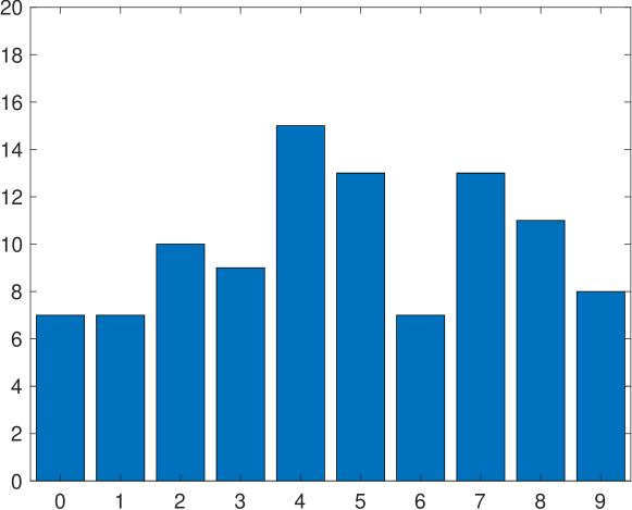
Figure 9: The histogram of the handwritten digits associated with the labeled samples after labeling $100$ samples. The first histogram is for the selection criterion $\mathsf{score}_{\mathcal{H}}$ and the second histogram is for the selection criterion $\mathsf{score}_{\mathtt{D}}$. Notably, $\mathsf{score}_{\mathcal{H}}$ has not labeled any of the images of the digit $0$.

6 Interpolating Neural Network Active Learners

Here we briefly examine the extension of the max-min criterion and its variants to neural network learners. Neural network complexity or capacity can be controlled by limiting magnitude of the network weights [24, 25, 26]. A number of weight norms and related measures have been recently proposed in the literature [27, 28, 29, 30, 31]. For example, ReLU networks with a single hidden layer and minimum $\ell_{2}$ norm weights coincide with linear spline interpolation [32]. With this in mind, we provide empirical evidence showing that defining the max-min criterion with the norm of the network weights yields a neural network active learning algorithm with properties analagous to those obtained in the RKHS setting.

Consider a single hidden layer network with ReLU activation units trained using MSE loss. In Figure 10 we show the results of an experiment implemented in PyTorch in the same settings considered above for kernel machines in Figures 3 and 4. We trained an overparameterized network with $100$ hidden layer units to perfectly interpolate four training points with locations and binary labels as depicted in Figure 10(a). The color depicts the magnitude of the learned interpolating function: dark blue is $0$ indicating the “decision boundary” and bright yellow is approximately $3.5$. Figure 10(b) denotes the $\mathsf{score}_{\mathcal{H}}$ with the weight norm (i.e., the $\ell_{2}$ norm of the resulting network weights when a new sample is selected at that location). The brightest yellow indicates the highest score and the location of the next selection. Figure 10(c) denotes the $\mathsf{score}_{\mathtt{D}}$ with the data-based norm defined in Equation (7). In both cases, the max occurs at roughly the same location, which is near the current decision boundary and closest to oppositely labeled points. The data-based norm also places higher scores on points further away from the labeled examples. Thus, the data selection behavior of the neural network is analagous to that of the kernel-based active learner (compare with Figure 3).

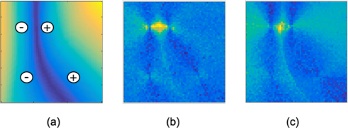
Figure 10: Data selection of neural network active learner. (a) Magnitude of output map of single hidden layer ReLU network trained to interpolate four data points as indicated (dark blue is $0$ indicating the learned decision boundary). (b) Max-Min selection of next point to label using network weight norm. (c) Max-Min selection of next point to label using data-based norm. Both select the point on the decision boundary that is closest to oppositely labeled examples.

Next we present a modified scenario in which the examples are not uniformly distributed over the input space, but instead concentrated only in certain regions indicated by the magenta highlights in Figure 11(a). In this setting, the example selection criteria differ more significantly for the two norms. The weight norm selection criterion remains unchanged, but is applied only to regions where there are examples. Areas without examples to select are indicated by dark blue in Figure 11(b)-(c). The data-based norm is sensitive to the non-uniform input distribution, and it scores examples near the lower portion of the decision boundary highest. Again, this is quite similar to the behavior of the kernel active learner (compare with Figure 4).

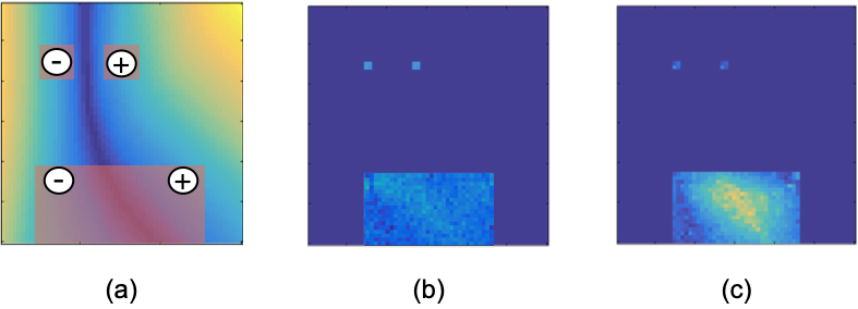
Figure 11: Data selection of neural network active learner. (a) Unlabeled examples are only available in magenta shaded regions. (b) Max-Min selection map using network weight norm. (c) Max-Min selection map using data-based norm.

7 Conclusion and Future Work

The question of designing active learning algorithms in the regime of nonparametric and overparameterized models become more essential as we look at larger models which require bigger training sets. To reduce the human cost of labeling all samples, we can use a pool-based active learning algorithm to avoid labeling non-informative examples.

Our algorithm does not exploit any assumption about the underlying classifier in selecting the samples to label. Yet, for a wide range of classifiers, it performs well with provable guarantees. It is designed for the extreme case of the nonparametric setting in which no assumption about the smoothness of the boundary between different classes is made by the learner.

There are many interesting questions remaining: the behavior of our proposed criterion applied to other classifiers such as kernel SVM instead of minimum norm interpolators, generalization of the criterion to multi-class settings and regression algorithms. The computational complexity of our criterion can also be a serious bottleneck in applications with bigger data-sets and should be addressed in future. Additional numerical simulations, especially with more complex architecture of Neural Networks can also be insightful.

Appendix A Maximin active learning with neural networks

We present the proof of Theorems 2 and 3 assuming the solutions to (2) and (3) – minimum norm interpolating functions – are linear spline functions with knots at each data point. According to Theorem 1, there are other solutions to the minimum “norm” neural network; but since $\mathsf{score}^{(1)}_{\mathcal{F}}$ only depends on the “norm” it suffices to just consider the spline case. Moreover, as shown in [21], the weight norm $\|f\|_{\mathcal{F}}:=\|{\boldsymbol{w}}\|_{2}$ is equal to the total variation of $f$. The total variation of a linear spline is the sum of the absolute values of the slopes of each linear piece. We use this equivalence throughout the proof.

For a linear spline function $f(x)$ with knots at each data point, the assumption $f(\infty)=f(-\infty)=0$ guarantees that for any $x_{i}$ such that $y_{i}=+1$, we have

$$\lim_{x\to x_{i}^{-}}\frac{\mathrm{d}}{\mathrm{d}x}f(x) \geq 0,\quad\quad\lim_{x\to x_{i}^{+}}\frac{\mathrm{d}}{\mathrm{d}x}f(x)\leq 0$$

Similarly, for any $x_{i}$ such that $y_{i}=+1$, we have

$$\lim_{x\to x_{i}^{-}}\frac{\mathrm{d}}{\mathrm{d}x}f(x) \leq 0,\quad\quad\lim_{x\to x_{i}^{+}}\frac{\mathrm{d}}{\mathrm{d}x}f(x)\geq 0$$

The assumption $f(\infty)=f(-\infty)=0$ also guarantees that $f^{\prime}(\infty)=f^{\prime}(-\infty)=0$.

Also, if a point $u$ is between two labeled points $x_{1}$ and $x_{2}$ such that $x_{1}<x_{2}$, then for any label $\ell\in\{-,1+1\}$ we know that $f^{u}_{\ell}(x)=f(x)$ for $x\leq x_{1}$ or $x\geq x_{2}$. Using these properties, we find the maximizer of $\mathsf{score}_{\mathcal{F}}(u)$ and $\mathsf{score}_{\mathtt{D}}(u)$ in various cases.

A.1 Maximin Criterion with Function Norm and Neural Networks (Proof of Theorem 2)

To prove Theorem 1, [20] shows that optimizing the parameters of a two layer Neural Network as described in Theorem 1 to find $\min_{\mathbf{w}}\|\mathbf{w}\|_{2}$ such that $f(x_{i})=y_{i}$ for all $i$ is the same as minimizing the $R(f)$ such that $f(x_{i})=y_{i}$ for all $i$ where $R(f)$ is defined as

$$R(f)=\max\Big{(}\big{|}f^{\prime}(+\infty)+f^{\prime}(-\infty)\big{|},\,\int|f^{\prime\prime}(x)|\,\mathrm{d}x\Big{)}\,.$$

Hence, we can use $R(f)$, as a proxy for a function norm in the context of Neural Networks.

In our setup, adding two artificial points to the left and right with the same labels as the true end points ensures that the function $R(f)=\int|f^{\prime\prime}(x)|\,\mathrm{d}x$ since $f^{\prime}(+\infty)=f^{\prime}(-\infty)=0$ for the minimum norm interpolating functions.

Hence, for a set of points $\{(x_{i},y_{i})\}_{i}$, the norm of minimum norm interpolating function is the same as $R(f)=\int|f^{\prime\prime}(x)|\,\mathrm{d}x$, i.e., “the summation of changes in the slope of minimal knot linear spline interpolation of points”. This quantity is used to compute the score of each unlabeled point. Note that clearly to compute the score of a point $u$ such that $x_{j}<u<x_{j+1}$, we only need to compute how much the slope of interpolating function changes by adding $u$ in the interval $x_{j}$ to $x_{j+1}$. In particular,

$$\|f^{u}_{\ell}(x)\|_{\mathcal{F}}-\|f(x)\|_{\mathcal{F}}=2\frac{1-\ell y_{j}}{u-x_{j}}+2\frac{1-\ell y_{j+1}}{x_{j+1}-u}-2\frac{1-y_{j}y_{j+1}}{x_{j+1}-x_{j}}\,.$$

1. Without loss of generality, assume $y_{1}=+1$ and $y_{2}=-1$. Hence,

   $$\lim_{x\to x_{1}^{-}}\frac{\mathrm{d}}{\mathrm{d}x}f(x)\geq 0$$

   and

   $$\lim_{x\to x_{2}^{+}}\frac{\mathrm{d}}{\mathrm{d}x}f(x)\geq 0\,.$$

   Looking at $f(x)$, we also have the slope of function between $x_{1}$ and $x_{2}$ to be $-\frac{2}{x_{2}-x_{1}}$.

   The same statements hold for $f_{\ell}^{u}(x)$ for any $x_{1}<u<x_{2}$ and $\ell\in\{-1,+1\}$.

   $$\lim_{x\to x_{1}^{-}}\frac{\mathrm{d}}{\mathrm{d}x}f_{\ell}^{u}(x) \geq 0\,,\quad\quad\lim_{x\to x_{2}^{+}}\frac{\mathrm{d}}{\mathrm{d}x}f_{\ell}^{u}(x)\geq 0\,.$$

   For $\ell=+1$, the slope of $f_{\ell}^{u}(x)$ for $x_{1}<x<u$ is zero and the slope of $f_{\ell}^{u}(x)$ for $u<x<x_{2}$ is $-\frac{2}{x_{2}-u}$. Since $f^{u}_{+}(x)=f(x)$ for $x\leq x_{1}$ or $x\geq x_{2}$,

   $$\|f(x)\|_{\mathcal{F}}-\frac{4}{x_{2}-x_{1}} =\|f^{u}_{+}(x)\|_{\mathcal{F}}-\frac{4}{x_{2}-u}\,.$$

   Using a similar calculation for $\ell=-1$ we get

   $$\|f^{u}_{+}(x)\|_{\mathcal{F}} =\|f(x)\|_{\mathcal{F}}-\frac{4}{x_{2}-x_{1}}+\frac{4}{x_{2}-u}\,,$$

   $$\|f^{u}_{-}(x)\|_{\mathcal{F}} =\|f(x)\|_{\mathcal{F}}-\frac{4}{x_{2}-x_{1}}+\frac{4}{u-x_{1}}\,.$$

   Hence, $\|f^{u}_{+}(x)\|_{\mathcal{F}}\geq\|f^{u}_{-}(x)\|_{\mathcal{F}}$ if and only if $u\geq\frac{x_{1}+x_{2}}{2}$ and

   $$\mathsf{score}_{\mathcal{F}}(u)=\|f^{u}(x)\|_{\mathcal{F}} =\|f(x)\|_{\mathcal{F}}-\frac{4}{x_{2}-x_{1}}+\min\Big{\{}\frac{4}{x_{2}-u},\frac{4}{u-x_{1}}\Big{\}}\,.$$ (15)

   This gives

   $$u^{*}:=\mathrm{argmax}_{x_{1}<u\leq x_{2}}\mathsf{score}^{(1)}_{\mathcal{F}}(u)=\frac{x_{1}+x_{2}}{2}\,.$$

   and

   $$\mathsf{score}_{\mathcal{F}}(u^{*})=\|f(x)\|_{\mathcal{F}}+\frac{4}{x_{2}-x_{1}}\,.$$

2. Above computation shows that pair of neighboring oppositely labeled points $x_{1}<x_{2}$ and $x_{3}<x_{4}$, if $x_{2}-x_{1}\geq x_{4}-x_{3}$, then

   $$\mathsf{score}_{\mathcal{F}}\big{(}\frac{x_{3}+x_{4}}{2}\big{)}\geq\mathsf{score}_{\mathcal{F}}\big{(}\frac{x_{1}+x_{2}}{2}\big{)}\,.$$

3. Assume $y_{5}=y_{6}=y$. Then, for $x_{5}\leq v\leq x_{6}$ we have $f^{v}_{y}(x)=f(x)$ for all $x$. For $\ell=-y$, we have

   $$\|f^{v}_{-y}(x)\|_{\mathcal{F}}=\|f(x)\|_{\mathcal{F}}+\frac{4}{u-x_{5}}+\frac{4}{x_{6}-u}\,.$$

   Hence, $\|f^{v}_{y}(x)\|_{\mathcal{F}}\leq\|f^{v}_{-y}(x)\|_{\mathcal{F}}$ and $f^{v}(x)=f^{v}_{y}(x)$. Hence, for a pair of identically labeled points $x_{5}$ and $x_{6}$ and all $x_{5}\leq v\leq x_{6}$, we have

   $$\mathsf{score}_{\mathcal{F}}(v)=\|f^{v}(x)\|_{\mathcal{F}}=\|f(x)\|_{\mathcal{F}}$$ (16)

   which is a constant independent of $v$.

4. Equations (15) and (16), show that in this setup

   $$\mathsf{score}_{\mathcal{F}}(v)=\|f(x)\|_{\mathcal{F}}\leq\mathsf{score}^{(1)}_{\mathcal{F}}(u)\,.$$

A.2 Proof of Theorem 3

Without loss of generality, assume $x_{1}=0$ and $x_{2}=1$. Then, if $y_{1}=y_{2}$, the statement of theorem is trivial.

Hnce,

$$f(x)=\frac{x_{2}+x_{1}-2x}{x_{2}-x_{1}}\,,\quad\text{ for all }x_{1}<x<x_{2}\,.$$

For $x_{1}<u<x_{2}$, we have $\ell(u)=+1$ if $x_{1}<u<(x_{1}+x_{2})/2$ and $\ell(u)=-1$ if $(x_{1}+x_{2})/2<u<x_{2}$. First, we look at $x_{1}<u<(x_{1}+x_{2})/2$:

$$f^{u}(x)=\begin{cases}1\,,\quad&\text{ for all }x_{1}<x<u\\ \frac{x_{2}+u-2x}{x_{2}-u}\,,\quad&\text{ for all }u<x<x_{2}\,.\end{cases}$$

Hence, for $x_{1}<u<(x_{1}+x_{2})/2$

$$\|f-f^{u}\|_{\mathtt{D}} =\int_{x_{1}}^{x_{2}}\big{[}f^{u}(x)-f(x)\big{]}^{2}\mathrm{d}x$$

$$=\frac{4}{(x_{2}-x_{1})^{2}}\int_{x_{1}}^{u}(x-x_{1})^{2}\mathrm{d}x+\frac{4(u-x_{1})^{2}}{(x_{2}-x_{1})^{2}(x_{2}-u)^{2}}\int_{u}^{x_{2}}(x_{2}-x)^{2}\mathrm{d}x$$

$$\frac{\mathrm{d}}{\mathrm{d}u}\|f-f^{u}\|_{\mathtt{D}} =\frac{4}{(x_{2}-x_{1})^{2}}(u-x_{1})^{2}-\frac{4(u-x_{1})^{2}}{(x_{2}-x_{1})^{2}(x_{2}-u)^{2}}(x_{2}-u)^{2}$$

$$\quad+\frac{8(u-x_{1})}{3(x_{2}-x_{1})(x_{2}-u)^{3}}(x_{2}-u)^{3}$$

$$=\frac{8}{3}\frac{u-x_{1}}{x_{2}-x_{1}}\geq 0\,.$$

Similarly, we can show that for $\frac{x_{1}+x_{2}}{2}\leq u\leq x_{2}$, $f^{u}(x)=f^{u}_{-}(x)$ and

$$\frac{\mathrm{d}}{\mathrm{d}u}\|f-f^{u}\|_{\mathtt{D}}\leq 0\,.$$

Appendix B Maximin kernel based active learning in one dimension

B.1 Minimum norm interpolating function with Laplace Kernel in one dimension

We want to find the minimum norm interpolating function based on set of labeled samples $\mathcal{L}=\{(x_{1},y_{1}),\cdots,(x_{n},y_{n})\}$ such that $x_{1}<x_{2}<\cdots,x_{n}$.

First, let us look at the Kernel matrix for three neighboring points $x_{1}<x_{2}<x_{3}$ according to the Laplace Kernel.

$$K =\begin{bmatrix}1&e^{-(x_{2}-x_{1})/h}&e^{-(x_{3}-x_{1})/h}\\ e^{-(x_{2}-x_{1})/h}&1&e^{-(x_{3}-x_{2})/h}\\ e^{-(x_{3}-x_{1})/h}&e^{-(x_{3}-x_{2})/h}&1\end{bmatrix}\,.$$

We define $d_{1}=e^{-(x_{2}-x_{1})/h}$ and $d_{2}=e^{-(x_{3}-x_{2})/h}$. It can be shown that with the above structure

$$K^{-1} =\begin{bmatrix}\frac{1}{1-d_{1}^{2}}&\frac{-d_{1}}{1-d_{1}^{2}}&0\\ \frac{-d_{1}}{1-d_{1}^{2}}&\frac{1}{1-d_{1}^{2}}+\frac{1}{1-d_{2}^{2}}-1&\frac{-d_{2}}{1-d_{2}^{2}}\\ 0&\frac{-d_{2}}{1-d_{2}^{2}}&\frac{1}{1-d_{2}^{2}}\\ \end{bmatrix}\,.$$

In general, if we look into the Kernel matrix for the set of points $x_{1}<x_{2}<\cdots<x_{n}$, and define $d_{i}=e^{-(x_{i+1}-x_{i})/h}$ for $1\leq i\leq n-1$. We define $d_{0}=d_{n}=0$. Using induction, on can show that the inverse of the Kernel matrix has a block diagonal form such that

$$(K^{-1})_{1,1} =\frac{1}{1-d_{1}^{2}},\quad\quad\quad(K^{-1})_{n,n}=\frac{1}{1-d_{n-1}^{2}}$$

$$(K^{-1})_{i,i} =\frac{1}{1-d_{i-1}^{2}}+\frac{1}{1-d_{i}^{2}}-1,\quad\quad\forall 1<i<n$$

$$(K^{-1})_{i,i+1} =(K^{-1})_{i+1,i}=\frac{-d_{i}}{1-d_{i}^{2}},\quad\quad\forall 1\leq i<n$$ (17)

and the remaining elements of matrix of matrix $K^{-1}$ is zero, i.e., $(K^{-1})_{i,j}$ for $|j-i|\geq 2$.

Using (10) and the above characterization of matrix $\textbf{K}^{-1}$, we can show that the the minimum norm interpolating function based on set of labeled samples $\mathcal{L}=\{(x_{1},y_{1}),\cdots,(x_{n},y_{n})\}$ such that $x_{1}<x_{2}<\cdots,x_{n}$ has the following form:

$$f(x) =\frac{1}{1+y_{1}y_{2}\,d_{1}}\,y_{1}k(x_{1},x)+\frac{1}{1+y_{n}y_{n_{1}}\,d_{n-1}}\,y_{n}k(x_{n},x)$$

$$\quad+\sum_{i=2}^{n-1}\Big{[}\frac{1}{1+y_{i}y_{i-1}d_{i-1}}+\frac{1}{1+y_{i}y_{i+1}d_{i}}-1\Big{]}\,y_{i}k(x_{i},x)\,.$$ (18)

B.2 Criterion $\mathsf{score}_{\mathcal{H}}$ with Laplace Kernel in one dimension (Proposition 2)

Proof of Proposition 1.

Looking at three neighboring points $x_{1}<x_{2}<\cdots<x_{n}$ labeled $\mathbf{y}=\{y_{1},y_{2},\cdots,y_{n}\}$, let $K$ be the kernel matrix corresponding to $\{x_{1},x_{2},\cdots,x_{n}\}$. Then, using the block diagonal structure given in Equation (17), we compute $\|f(x)\|_{\mathcal{H}}$:

$$\|f(x)\|_{\mathcal{H}} =\mathbf{y}^{T}K^{-1}\mathbf{y}$$

$$=\mathsf{trace}(K^{-1})+\sum_{i=1}^{n-1}2y_{i}y_{i+1}(K^{-1})_{i,i+1}$$

$$=-(n-2)+2\sum_{i=1}^{n-1}\frac{1-y_{i}y_{i+1}\exp(-(x_{i+1}-x_{i})/h)}{1-\exp(-2(x_{i+1}-x_{i})/h)}$$

$$=-(n-2)+2\sum_{i=1}^{n-1}\frac{1}{1+y_{i}y_{i+1}\exp(-(x_{i+1}-x_{i})/h)}\,.$$ (19)

This factorization of $\|f(x)\|_{\mathcal{H}}$ implies that if $x_{i}<u<x_{j+1}$, we have

$$\|f_{\ell}^{u}(x)\|_{\mathcal{H}}= \|f(x)\|_{\mathcal{H}}-1-\frac{2}{1+y_{j}y_{j+1}\exp(-(x_{j+1}-x_{j})/h)}$$

$$+\frac{2}{1+\ell y_{j}\exp(-(u-x_{j})/h)}+\frac{2}{1+\ell y_{j+1}\exp(-(x_{j+1}-u)/h)}\,.$$ (20)

This factorization of $\|f_{\ell}^{u}(x)\|_{\mathcal{H}}$ implies that given $n$ labeled points, to find the global maximizer of $\mathsf{score}_{\mathcal{H}}(u)$, the following strategy works:

Step 1: For each $j$, we find the maximizer of $\mathsf{score}_{\mathcal{H}}(u)$ for the unlabeled points $u$ such that $x_{j}<u<x_{j+1}$. We define

$$u_{j}^{*}=\arg\max_{x_{j}<u<x_{j+1}}\mathsf{score}_{\mathcal{H}}(u)$$ (21)

The above factorization (20) shows that to find $u_{j}^{*}$, we can alternatively find the maximizer of the sore given a configuration of only two labeled points $\mathcal{L}^{\prime}=\{(x_{i},y_{j}),(x_{j+1},y_{j+1})\}$ and unlabeled points $x_{j}<u<x_{j+1}$ to find the maximizer of the last two terms of the above factorization. The maximzer of $\mathsf{score}_{\mathcal{H}}(u)$ for $u$ such that $x_{j}<u<x_{j+1}$ given $\mathcal{L}^{\prime}$ is the same as the maximizer of $\mathsf{score}_{\mathcal{H}}(u)$ for $u$ such that $x_{j}<u<x_{j+1}$ given $\mathcal{L}$.

Step 2: Note that $\arg\max_{u}\mathsf{score}_{\mathcal{H}}(u)=u_{j^{*}}^{*}$ such that $j^{*}=\arg\max_{j}\mathsf{score}_{\mathcal{H}}(u_{j}^{*})$. We can use (20) to compare $\mathsf{score}_{\mathcal{H}}(u_{j}^{*})$ for various values of $j$.

In what follows, we show that using Laplace Kernel, whether $y_{j}=y_{j+1}$ or $y_{j}\neq y_{j+1}$, we always have $u_{j}^{*}=(x_{j}+x_{j+1})/2$ and $\ell(u_{j}^{*})=y_{j}$. Hence, using (20), we have

$$\mathsf{score}_{\mathcal{H}}(u_{j}^{*})= \|f(x)\|_{\mathcal{H}}-1-\frac{2}{1+y_{j}y_{j+1}\exp(-(x_{j+1}-x_{j})/h)}$$

$$+\frac{2}{1+\exp(-(x_{j+1}-x_{j})/2h)}+\frac{2}{1+y_{j}y_{j+1}\exp(-(x_{j+1}-x_{j})/2h)}\,.$$ (22)

Step 1:

1. Consider two neighboring points $x_{1}<x_{3}$ labeled $\mathbf{y}=\{-,+\}$. Let $u$ be such that $x_{1}<u<x_{3}$ and $t=y_{3}$. Define $A=e^{-(u-x_{1})/h}$ and $B=e^{-(x_{3}-u)/h}$. Define the matrix $K$ to be the kernel matrix corresponding to the points $x_{1},u,x_{3}$. Then using (19)

   $$\|f^{u}_{\ell}(x)\|^{2} =\frac{2}{1-\ell A}+\frac{2}{1+\ell B}-1$$

   Hence,

   $$\ell(u) =\mathrm{argmin}_{\ell}\|f^{u}_{\ell}(x)\|^{2}=\begin{cases}+1,\quad\quad\text{if }u>\frac{x_{1}+x_{3}}{2}\text{ or }B>A\\ -1,\quad\quad\text{if }u\leq\frac{x_{1}+x_{3}}{2}\text{ or }B\leq A\end{cases}$$

   Without loss of generality, assume $A\geq B$ or $u\leq\frac{x_{1}+x_{3}}{2}$, then the block diagonal structure given in Equation (17) implies

   $$\mathsf{score}_{\mathcal{H}}(u) =2\left\{\frac{1}{1+A}+\frac{1}{1-B}\right\}-1$$

   Note that for all $u$ such that $x_{1}<u<x_{3}$, we have $AB=e^{-(x_{3}-x_{1})/h}=C$ and is constant. So

   $$\max_{u\leq\frac{x_{1}+x_{3}}{2}}\mathsf{score}_{\mathcal{H}}(u) =\max_{A,B,\text{ s.t. }AB=C,A\geq B}2\left\{\frac{1}{1+A}+\frac{1}{1-B}\right\}-1$$

   $$=\frac{4}{1-C}-1=\frac{4}{1-e^{-(x_{3}-x_{1})/h}}-1$$

   which is attained when $A=B$ or $u=\frac{x_{1}+x_{3}}{2}$.

   This gives the following statement: For neighboring labeled points $x_{1}<x_{3}$ such that $y_{1}\neq y_{3}$, we have

   $$\max_{s_{1}\leq u\leq x_{3}}\mathsf{score}_{\mathcal{H}}(u)=\mathsf{score}_{\mathcal{H}}(\frac{x_{1}+x_{3}}{2})=\frac{4}{1-e^{-(x_{3}-x_{1})/h}}-1\,.$$ (23)

   Note that the above function is decreasing in $x_{3}-x_{1}$.

2. Consider two neighboring points $x_{1}<x_{3}$ labeled $\mathbf{y}=\{+,+\}$. Let $u$ such that $x_{1}<u<x_{3}$ and $t=y_{3}$. Define $A=e^{-(u-x_{1})/h}$ and $B=e^{-(x_{3}-u)/h}$.

   $$\max_{x_{1}<u<x_{3}}\mathsf{score}_{\mathcal{H}}(u) =\max_{A,B,\text{ s.t. }AB=C}2\left\{\frac{1}{1+A}+\frac{1}{1+B}\right\}-1$$

   $$=\frac{4}{1+\sqrt{C}}-1=\frac{4}{1+{e^{-(x_{3}-x_{1})/2h}}}-1$$

   This gives the following statement: For neighboring labeled points $x_{1}<x_{3}$ such that $y_{1}=y_{3}$, we have

   $$\max_{s_{1}\leq u\leq x_{3}}\mathsf{score}_{\mathcal{H}}(u)=\mathsf{score}_{\mathcal{H}}(\frac{x_{1}+x_{3}}{2})=\frac{4}{1+{e^{-(x_{3}-x_{1})/2h}}}-1\,.$$ (24)

   Note that the above function is increasing in $x_{3}-x_{1}$.

Step 2: In Step 1, we showed that the maximizer of score at each interval between two neighboring points is achieved in the center of the interval, i.e., $u^{*}_{j}=\frac{x_{j}+x_{j+1}}{2}$ with notation defined in (21). Now to compare $\mathsf{score}_{\mathcal{H}}(u^{*}_{j})$ for various $j$, we look at the following properties derived from the formulation in (22):

• If $y_{j}\neq y_{j+1}$, then

  $$\mathsf{score}_{\mathcal{H}}(u^{*}_{j})=\|f(x)\|_{\mathcal{H}}-1+\frac{2}{1-\exp(-(x_{j+1}-x_{j})/h)}\geq\|f(x)\|_{\mathcal{H}}+1\,.$$

  Note that if $y_{j}\neq y_{j+1}$, then $\mathsf{score}_{\mathcal{H}}(u^{*}_{j})$ is increasing in $x_{j+1}-x_{j}$.

• If $y_{j}=y_{j+1}$, then

  $$\mathsf{score}_{\mathcal{H}}(u^{*}_{j})=\|f(x)\|_{\mathcal{H}}-1-\frac{2}{1+\exp(-(x_{j+1}-x_{j})/h)}+\frac{4}{1+\exp(-(x_{j+1}-x_{j})/2h)}\leq\|f(x)\|_{\mathcal{H}}+1\,.$$

  Note that if $y_{j}=y_{j+1}$, then $\mathsf{score}_{\mathcal{H}}(u^{*}_{j})$ is decreasing in $x_{j+1}-x_{j}$.

The above two properties give the statement of the second part of proposition. ∎

B.3 Max Min criteria Binary Search (Corollary 2)

According to the last property in Proposition 2 the first sample selected will be at the midpoint of the unit interval and the second point will be at $1/4$ or $3/4$. If the labels agree, then the next sample will be at the midpoint of the largest subinterval (e.g., at $3/4$ if $1/4$ was sampled first). Sampling at the midpoints of the largest subinterval between a consecutive pairs labeled points continues until a point with the opposite label is found. Once a point the with opposite label have been found, Proposition 2 implies that subsequent samples repeatedly bisect the subinterval between the closest pair of oppositely labeled points. This bisection process will terminate with two neighboring points having opposite labels, thus identifying one boundary/threshold of $g$. The total number of labels collected by this bisection process is at most $\log_{2}N$. After this, the algorithm alternates between the two situations above. It performs bisection on the subinterval between the close pair of oppositely labeled points, if such an interval exists. If not, it samples at the midpoint of the largest subinterval between a consecutive pairs of labeled points. The stated label complexity bound follows from the assumptions that there are $K$ thresholds and the length of each piece (subinterval between thresholds) is on the order of $1/K$.

B.4 One Dimensional Functions with Radial Basis Kernels (Proposition 3)

Proof of Proposition 3 on maximum score with radial basis kernels.

For the ease of notation, for fixed $p$ and $h$, we define $a,b>0$ as the normalized distance between samples such that $x_{2}-x_{1}=bh^{1/p}$ and $x_{3}-x_{2}=ah^{1/p}$. For $x_{2}<u<x_{3}$, we define $0<c<a$ such that the distance between the point $u$ and $x_{2}$ is $u-x_{2}=ch^{1/p}$, as in Figure 12. The proposition is based on the assumption that for any pair of points, $|x-x^{\prime}|\geq\Delta$ and $h$ is sufficiently small that $a,b,c,a-c\geq\Delta h^{-1/p}$.

We want to show that the max score happens at the zero crossing of function $f(u)$. Since we normalized all pairwise distances by $h^{1/p}$, instead we will show that there exists a constant $D$ such that if $a,b,c,a-c\geq D$, then the max score is achieved at the zero crossing.

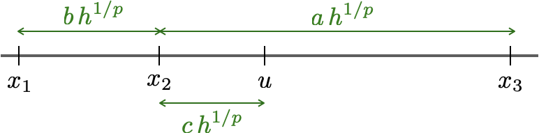
Figure 12: The samples $x_{1},x_{2}$ and $x_{3}$ are the labeled samples such that $y_{1}=y_{2}=+1$ and $y_{3}=-1$.

Note that $\|f^{(u)}_{+}\|$ depends on the location of point $u$, characterized by the normalized distance between $u$ and $x_{2}$ denoted by $c$. We want to prove that for small enough bandwidth, $\|f^{(u)}_{+}\|$ is increasing in $c$ for $\Delta h^{-1/p}<c<a-\Delta h^{-1/p}$. We can use similar argument to show that $\|f^{(u)}_{-}\|$ is decreasing in $c$. This implies

$$\max_{\Delta h^{-1/p}<c<a-\Delta h^{-1/p}}\,\,\,\,\min_{\ell\in\{\-,+\}}\|f^{(u)}_{\ell}\|=\|f^{(u^{*})}_{+}\|=\|f^{(u^{*})}_{-}\|$$

with $u^{*}$ defined to be the point in which $f(u^{*})=0$.

To do so, we will show that $\frac{\mathrm{d}}{\mathrm{d}c}\|f^{(u)}_{+}\|>0$ in the interval $\Delta h^{-1/p}<c<a-\Delta h^{-1/p}$.

In the proof of Proposition 1, we showed the following form for the function $\|f^{(u)}_{+}\|$,

$$\|f^{u}_{+}(x)\|=\frac{\big{[}1-\,f(u)\big{]}^{2}}{1-\textbf{a}_{u}^{T}\,\textbf{K}^{-1}\textbf{a}_{u}}$$

where K is the kernel matrix for the points $x_{1},x_{2}$ and $x_{3}$. The vector $\textbf{a}_{v}$ is defined to be $\textbf{a}_{v}=[K(x_{1},u),K(x_{2},u),K(x_{3},u)]^{T}$. The term $f(u)$ is the minimum norm interpolating function based on the points $x_{1},x_{2}$ and $x_{3}$ and their labels evaluated at $u$. Equation 10 shows that

$$f(u)=\textbf{y}^{T}\textbf{K}^{-1}\textbf{a}_{u}\,.$$

First, we look at K and its inverse in the setup explained above. Using the definition of Radial basis kernels in Equation (4),

$$\mathbf{K}=\begin{bmatrix}1&\exp(-b^{p})&\exp[-(a+b)^{p}]\\ \exp(-b^{p})&1&\exp(-a^{p})\\ \exp[-(a+b)^{p}]&\exp(-a^{p})&1\end{bmatrix}$$ (25)

Hence,

$$\mathbf{K}^{-1} =\frac{1}{|\mathbf{K}|}\begin{bmatrix}1-e^{-2a^{p}}&&-e^{-b^{p}}+e^{-a^{p}-(b+a)^{p}}&&e^{-a^{p}-b^{p}}-e^{-(a+b)^{p}}\\ \\ -e^{-b^{p}}+e^{-a^{p}-(b+a)^{p}}&&1-e^{-2(a+b)^{p}}&&-e^{-a^{p}}+e^{-b^{p}-(a+b)^{p}}\\ \\ e^{-a^{p}-b^{p}}-e^{-(a+b)^{p}}&&-e^{-a^{p}}+e^{-b^{p}-(a+b)^{p}}&&1-e^{-2b^{p}}\end{bmatrix}$$

$$=\frac{1}{|\mathbf{K}|}\begin{bmatrix}1-e^{-2a^{p}}&&-e^{-b^{p}}[1-\epsilon_{1}]&&e^{-a^{p}-b^{p}}[1-\epsilon_{2}]\\ \\ -e^{-b^{p}}[1-\epsilon_{1}]&&1-e^{-2(a+b)^{p}}&&-e^{-a^{p}}[1-\epsilon_{3}]\\ \\ e^{-a^{p}-b^{p}}[1-\epsilon_{2}]&&-e^{-a^{p}}[1-\epsilon_{3}]&&1-e^{-2b^{p}}\end{bmatrix}$$

The determinant of matrix K is

$$|\mathbf{K}| =1+2\exp[-a^{p}-b^{p}-(a+b)^{p}]-\exp[-2(a+b)^{p}]-\exp(-2a^{p})-\exp(-2b^{p}) =1-\epsilon^{\prime}$$

where we defined

$$\epsilon^{\prime} =\exp[-2(a+b)^{p}]+\exp(-2a^{p})+\exp(-2b^{p})-2\exp[-a^{p}-b^{p}-(a+b)^{p}]$$

$$\epsilon_{1} =\exp\big{(}{b^{p}-a^{p}-(b+a)^{p}}\big{)}$$

$$\epsilon_{2} =\exp\big{(}{b^{p}+a^{p}-(b+a)^{p}}\big{)}$$

$$\epsilon_{3} =\exp\big{(}{a^{p}-b^{p}-(b+a)^{p}}\big{)}$$

Note that since for $p\geq 1$, we have $(a+b)^{p}\geq a^{p}+b^{p}$, then $\epsilon^{\prime},\epsilon_{1},\epsilon_{2},\epsilon_{3}\geq 0$. Also, there exists a constant $D$ such that if $a,b>D$, then $|\textbf{K}|\geq 0.9$.

The vector $\textbf{a}_{v}$ is

$$\textbf{a}_{v} =[K(x_{1},u),K(x_{2},u),K(x_{3},u)]^{T}=\begin{bmatrix}\exp[-(c+b)^{p}]&\exp(-c^{p})&\exp[-(a-c)^{p}]\end{bmatrix}^{T}$$

Next, we compute $f(u)$

$$f(u) =\mathbf{y}^{T}\mathbf{K}^{-1}\textbf{a}_{u}$$

$$=\frac{1}{|\mathbf{K}|}\begin{bmatrix}1&1&-1\end{bmatrix}\begin{bmatrix}1-e^{-2a^{p}}&&-e^{-b^{p}}[1-\epsilon_{1}]&&e^{-a^{p}-b^{p}}[1-\epsilon_{2}]\\ \\ -e^{-b^{p}}[1-\epsilon_{1}]&&1-e^{-2(a+b)^{p}}&&-e^{-a^{p}}[1-\epsilon_{3}]\\ \\ e^{-a^{p}-b^{p}}[1-\epsilon_{2}]&&-e^{-a^{p}}[1-\epsilon_{3}]&&1-e^{-2b^{p}}\end{bmatrix}\begin{bmatrix}e^{-(c+b)^{p}}\\ \\ e^{-c^{p}}\\ \\ e^{-(a-c)^{p}}\end{bmatrix}$$

$$=\frac{1}{|\mathbf{K}|}\left\{e^{-(c+b)^{p}}[1-\epsilon_{4}]+e^{-c^{p}}[1-\epsilon_{5}]-e^{-(a-c)^{p}}[1-\epsilon_{6}]\right\}$$

where we defined

$$\epsilon_{4} =e^{-2a^{p}}+e^{-b^{p}}[1-\epsilon_{1}]+e^{-a^{p}-b^{p}}[1-\epsilon_{2}]$$

$$\epsilon_{5} =e^{-b^{p}}[1-\epsilon_{1}]+e^{-2(a+b)^{p}}-e^{-a^{p}}[1-\epsilon_{3}]$$

$$\epsilon_{6} =e^{-a^{p}-b^{p}}[1-\epsilon_{2}]-e^{-a^{p}}[1-\epsilon_{3}]+e^{-2b^{p}}$$

So there exists a constant $D$ such that if $a,b,c,a-c>D$, then $|f(u)|\leq 1$ and $\epsilon_{4},\epsilon_{5},\epsilon_{6}\leq 0.1$.

Next, we derive the derivative of $f(u)$ as a function of $c$

$$|\textbf{K}|\frac{\mathrm{d}}{\mathrm{d}c}f(u) =-p(c+b)^{p-1}e^{-(c+b)^{p}}[1-\epsilon_{4}]-p\,.c^{p-1}e^{-c^{p}}[1-\epsilon_{5}]-p(a-c)^{p-1}e^{-(a-c)^{p}}[1-\epsilon_{6}]\,.$$

$$\leq-0.9\big{\{}p\,.c^{p-1}e^{-c^{p}}+p(a-c)^{p-1}e^{-(a-c)^{p}}\big{\}}$$

where the last inequality uses $\epsilon_{4},\epsilon_{5},\epsilon_{6}\leq 0.1$.

Next, we compute $\textbf{a}_{u}^{T}\textbf{K}^{-1}\textbf{a}_{u}$ and its derivative with respect to $c$. To use the formulation computed in the proof of Proposition 1, we compute $\textbf{a}_{u}^{T}\mathbf{K}^{-1}\textbf{a}_{u}$ to be

$$|\textbf{K}|\textbf{a}_{u}^{T}\textbf{K}^{-1}\textbf{a}_{u} =e^{-2(b+c)^{p}}\big{[}1-e^{-2a^{p}}\big{]}+e^{-2c^{p}}\big{[}1-e^{-2(a+b)^{p}}\big{]}+e^{-2(a-c)^{p}}\,\big{[}1-e^{-2b^{p}}\big{]}$$

$$\quad-2\exp{\big{(}-b^{p}-c^{p}-(b+c)^{p}\big{)}}\,\,[1-\epsilon_{1}]$$

$$\quad+2\exp{\big{(}-b^{p}-a^{p}-(c+b)^{p}-(a-c)^{p}\big{)}}\,\,[1-\epsilon_{2}]$$

$$\quad-2\exp{\big{(}-a^{p}-c^{p}-(a-c)^{p}\big{)}}\,\,[1-\epsilon_{3}]$$

$$1-\textbf{a}_{u}^{T}\textbf{K}^{-1}\textbf{a}_{u} \geq 0.9$$

where the last inequality holds for large enough constant $D$ such that $a,b,c,a-c>D$. Hence,

$$|\textbf{K}|\frac{\mathrm{d}}{\mathrm{d}c}\textbf{a}_{u}^{T}\textbf{K}^{-1}\textbf{a}_{u} =-2p\,(b+c)^{p-1}e^{-2(b+c)^{p}}\big{[}1-e^{-2a^{p}}\big{]}$$

$$\quad-2pc^{p-1}e^{-2c^{p}}\big{[}1-e^{-2(a+b)^{p}}\big{]}+2p(a-c)^{p-1}e^{-2(a-c)^{p}}\,\big{[}1-e^{-2b^{p}}\big{]}$$

$$\quad+2p[c^{p-1}+(b+c)^{p-1}]\,\,\exp{\big{(}-b^{p}-c^{p}-(b+c)^{p}\big{)}}\,\,[1-\epsilon_{1}]$$

$$\quad-2p[(c+b)^{p-1}-(a-c)^{p-1}]\,\,\exp{\big{(}-b^{p}-a^{p}-(c+b)^{p}-(a-c)^{p}\big{)}}\,\,[1-\epsilon_{2}]$$

$$\quad+2p[c^{p-1}-(a-c)^{p-1}]\,\,\exp{\big{(}-a^{p}-c^{p}-(a-c)^{p}\big{)}}\,\,[1-\epsilon_{3}]$$

$$\big{|}\frac{\mathrm{d}}{\mathrm{d}c}\textbf{a}_{u}^{T}\textbf{K}^{-1}\textbf{a}_{u}\big{|} \leq 8pc^{p-1}e^{-2c^{p}}+8p(a-c)^{p-1}e^{-2(a-c)^{p}}$$

The remaining of the proof is based on the assumption that there exists a constant large enough value $D$ such that $a,b,c,a-c>D$. As we saw, this implies $f(u)<1$. Plugging in the above computations in to the derivative of the function $\|f^{u}_{+}(x)\|$ with respect to $c$, after doing some algebra, we see that this function is increasing in $c$. We give the sketch of this algebra here:

$$\frac{\mathrm{d}}{\mathrm{d}c}\|f^{u}_{+}(x)\| =\big{(}1-f(u)\big{)}\frac{-2(1-\textbf{a}_{u}^{T}\textbf{K}^{-1}\textbf{a}_{u})\,\frac{\mathrm{d}}{\mathrm{d}c}f(u)+\big{(}1-f(u)\big{)}\frac{\mathrm{d}}{\mathrm{d}c}\textbf{a}_{u}^{T}\textbf{K}^{-1}\textbf{a}_{u}}{(1-\textbf{a}_{u}^{T}\textbf{K}^{-1}\textbf{a}_{u})^{2}}$$

$$\geq\big{(}1-f(u)\big{)}\frac{1.5\big{\{}p\,.c^{p-1}e^{-c^{p}}+p(a-c)^{p-1}e^{-(a-c)^{p}}\big{\}}+\big{(}1-f(u)\big{)}\frac{\mathrm{d}}{\mathrm{d}c}\textbf{a}_{u}^{T}\textbf{K}^{-1}\textbf{a}_{u}}{(1-\textbf{a}_{u}^{T}\textbf{K}^{-1}\textbf{a}_{u})^{2}}$$

$$\geq 0\,.$$

The last inequality uses the bounds proved above.

Similarly, we can prove that $\|f^{u}_{-}(x)\|$ is decreasing in $c$. this implies that the $\mathsf{score}$ function is maximize in the zero crossing of function $f(x)$. ∎

Appendix C Maximin kernel based active learning with clustered data

To prove the statement of theorems presented in Section 4.6, we introduce some notations consistent with the notation introduced in Section 4.1. Given a set of labeled samples $\mathcal{L}=\{(x_{1},y_{1}),\cdots,(x_{L},y_{L})\}$, define the $L$ by $L$ matrix $\textbf{K}=[k(x_{i},x_{j})]_{1\leq i,j\leq L}$ and vector $\textbf{y}=[y_{1},\cdots,y_{L}]^{T}$.

Recall that $\mathcal{U}$ is a set of unlabled examples. For $u\in\mathcal{U}$ and $\ell\in\{-1,+1\}$, let $\textbf{a}_{u}=[k(x_{1},u),\cdots,k(x_{L},u)]^{T}$ and $\widetilde{\textbf{K}}_{u}$ be the $L+1$ by $L+1$ matrix such that

$$\widetilde{\textbf{K}}_{u}=\begin{bmatrix}\textbf{K}&\textbf{a}_{u}\\ \textbf{a}_{u}^{T}&1\end{bmatrix}\quad\text{and}\quad\widetilde{\textbf{y}}_{\ell}=\begin{bmatrix}\textbf{y}\\ t\end{bmatrix}\,.$$

Let $\mathcal{B}_{d,p}(r;c)$ be the $d$ dimensional $\ell_{p}$ ball with radius $r$ centered at $c$ (defined in (14)). Let $V_{d,p}(r)$ be the volume of $\mathcal{B}_{d,p}(r;0)$ with respect to the Lebesgue measure.

C.1 Proof of Theorem 4

The statement of theorem implies that when the data is clustered and distributed uniformly in $\ell_{p}$ balls, with centers far enough from each other, the first selected point using the $\mathsf{score}_{\mathtt{D}}$ function defined in (7) is in the largest ball. To prove this, we will show that the $\mathsf{score}_{\mathtt{D}}(c_{1})$, as defined in (7) is larger than $\mathsf{score}_{\mathtt{D}}(v)$ for any $v\notin B_{1}$ where $c_{1}$ is the center of $B_{1}$. Note that this does not imply that the first selected point coincides with the center of $B_{1}$. It guarantees that the largest ball contains at least one point with a score larger than that of every point in other balls.

Since $\mathcal{L}=\varnothing$, the empty set, the current interpolating function is uniformly zero everywhere $f(x)=0$ (according to the definition (10)). According to the Equations (3) and (4), for all $u\in\mathcal{U}$, we can choose $\ell(u)$ to be equal to $+1$ or $-1$. We choose $\ell(u)=+1$ without loss of generality for all $u\in\mathcal{U}$.

Using (10), adding any point $u\in\mathcal{U}$ with label $\ell(u)$ to $\mathcal{L}$ would give the new interpolating function

$$f^{u}(x):=f^{u}_{\ell(u)}(x)=k(u,x)=\exp\big{(}-\frac{1}{h}\|x-u\|_{p}\big{)}\,.$$

Hence, since $\mathbb{P}_{X}(x)$ is uniform over $\mathcal{X}=\cup_{i=1}^{M}B_{i}$

$$\mathsf{score}_{\mathtt{D}}(u) =\int_{x\in\mathcal{X}}\exp\big{(}-\frac{2}{h}\|x-u\|_{p}\big{)}\mathrm{d}P_{X}(x)=\frac{1}{V}\sum_{i=1}^{M}\int_{x\in B_{i}}\exp\big{(}-\frac{2}{h}\|x-u\|_{p}\big{)}\mathrm{d}x$$

where we defined $V=\sum_{i=1}^{M}V_{d,p}(r_{i})$ to be the total volume of $\mathcal{X}$. So, to compute $\mathsf{score}_{\mathtt{D}}(c_{1})$,

$$V\mathsf{score}_{\mathtt{D}}(c_{1}) =\sum_{i=1}^{M}\int_{x\in B_{i}}\exp\big{(}-\frac{2}{h}\|x-c_{1}\|_{p}\big{)}\,\mathrm{d}x\geq\int_{x\in B_{1}}\exp\big{(}-\frac{2}{h}\|x-c_{1}\|_{p}\big{)}\,\mathrm{d}x$$

$$=\int_{s=0}^{r_{1}}\exp\big{(}-\frac{2s}{h}\big{)}\,\mathrm{d}V_{d,p}(s)$$ (26)

where we used the change of variable $s=\|x-c_{1}\|_{p}$ in the last line.

For $v\notin B_{1}$, we want to show that $\mathsf{score}_{\mathtt{D}}(v)\leq\mathsf{score}_{\mathtt{D}}(c_{1})$. Let $v\in B_{j}$ such that $j\neq 1$.

$$V\mathsf{score}_{\mathtt{D}}(v) =\int_{x\in B_{j}}\exp\big{(}-\frac{2}{h}\|x-v\|_{p}\big{)}\mathrm{d}x+\sum_{i=1,i\neq j}^{M}\int_{x\in B_{i}}\exp\big{(}-\frac{2}{h}\|x-v\|_{p}\big{)}\mathrm{d}x$$ (27)

We will bound each of above terms separately.

For any $i\neq j$ and $x\in B_{i}$ application of triangle inequality gives

$$\|x-v\|_{p}\geq\|c_{i}-c_{j}\|-\|x-c_{i}\|-\|v-c_{j}\|\geq D$$

since $v\in B_{j},x\in B_{i}$ and $\|c_{i}-c_{j}\|_{p}\geq D+2r_{1}$, $\|x-c_{i}\|_{p}\leq r_{i}\leq r_{1}$ and $\|v-c_{j}\|_{p}\leq r_{j}\leq r_{1}$. Hence,

$$\sum_{i=1,i\neq j}^{M} \int_{x\in B_{i}}\exp\big{(}-\frac{2}{h}\|x-v\|_{p}\big{)}\mathrm{d}x\leq\sum_{i=1,i\neq j}^{M}\int_{x\in B_{i}}e^{-2D/h}\mathrm{d}x\leq e^{-2D/h}\sum_{i=1,i\neq j}^{M}V_{i}\,.$$ (28)

Lemma 1 shows that the first term in (27) is largest when $v$ coincides with $c_{j}$. Hence,

$$\int_{x\in B_{j}}\exp\big{(} -\frac{2}{h}\|x-v\|_{p}\big{)}\mathrm{d}x\leq\int_{x\in B_{j}}\exp\big{(}-\frac{2}{h}\|x-c_{j}\|_{p}\big{)}\mathrm{d}x=\int_{s=0}^{r_{j}}e^{-2s/h}\,\,\mathrm{d}V_{d,p}(s)\,.$$ (29)

Equations (26), (27), (28), and (29) give

$$V\mathsf{score}_{\mathtt{D}}(c_{1})-V\mathsf{score}_{\mathtt{D}}(v) \geq\int_{s=r_{j}}^{r_{1}}\exp\big{(}-\frac{2s}{h}\big{)}\,\,\mathrm{d}V_{d,p}(s)-\exp\big{(}-\frac{2}{h}D\big{)}\sum_{i=1,i\neq j}^{M}V_{i}$$

$$\geq\exp\big{(}-\frac{2r_{1}}{h}\big{)}\,\,\big{[}V_{1}-V_{j}\big{]}-M\,V_{1}\exp\big{(}-\frac{2D}{h}\big{)}\,.$$

Hence,

$$\frac{V}{V_{1}}\Big{[}\mathsf{score}_{\mathtt{D}}(c_{1})-\mathsf{score}_{\mathtt{D}}(v)\Big{]} \geq\exp\big{(}-\frac{2r_{1}}{h}\big{)}\,\,\big{[}1-\frac{V_{j}}{V_{1}}\big{]}-M\,\exp\big{(}-2\frac{D}{h}\big{)}$$

$$\stackrel{{\scriptstyle(a)}}{{\geq}}\exp\big{(}-\frac{2r_{1}}{h}\big{)}\,\,\big{[}1-\big{(}\frac{r_{2}}{r_{1}}\big{)}^{d}\big{]}-M\,\exp\big{(}-2\frac{D}{h}\big{)}\geq 0\,,$$

where inequality (a) is due to the property that

$$V_{d,p}(r)=\frac{\big{[}2r\,\Gamma(1+1/p)\big{]}^{d}}{\Gamma(1+d/p)}$$

and $r_{j}\leq r_{2}$ for all $j\neq 1$. Also, the assumption

$$D>\frac{h}{2}\Big{[}\ln M-\ln\big{(}1-(r_{2}/r_{1})^{d}\big{)}\Big{]},$$

and $r_{1}\leq h/2$ made in the statement of the theorem, yields the last inequality.

Lemma 1.

For any $v\in B=\mathcal{B}_{d,p}(r,c)$, we have

$$\int_{x\in B}\exp\Big{(}\frac{-\|x-v\|}{h}\Big{)}\,\mathrm{d}x\leq\int_{x\in B}\exp\Big{(}\frac{-\|x-c\|}{h}\Big{)}\,\mathrm{d}x\,.$$

Proof.

To prove the statement of lemma, instead of looking at the integration of two different functions $\exp\Big{(}\frac{-\|x-v\|}{h}\Big{)}$ and $\exp\Big{(}\frac{-\|x-c\|}{h}\Big{)}$ on one ball, we look at two balls each centered on $v$ and $c$. This intermediate steps helps up prove the statement of lemma.

Let $B_{1}=\mathcal{B}_{d,p}(r,c)$ and $B_{2}=\mathcal{B}_{d,p}(r,v)$. Then,

$$\int_{x\in B_{1}}\exp\Big{(}\frac{-\|x-c\|}{h}\Big{)}\,\mathrm{d}x=\int_{x\in B_{2}}\exp\Big{(}\frac{-\|x-v\|}{h}\Big{)}\,\mathrm{d}x\,.$$

Hence, to prove the statement of the lemma, we upper bound the following:

$$\int_{x\in B_{1}}\exp\Big{(}\frac{-\|x-v\|}{h}\Big{)}\,\mathrm{d}x -\int_{x\in B_{1}}\exp\Big{(}\frac{-\|x-c\|}{h}\Big{)}\,\mathrm{d}x$$

$$=\int_{x\in B_{1}}\exp\Big{(}\frac{-\|x-v\|}{h}\Big{)}\,\mathrm{d}x-\int_{x\in B_{2}}\exp\Big{(}\frac{-\|x-v\|}{h}\Big{)}\,\mathrm{d}x$$

$$=\int_{x\in B_{1}\setminus B_{2}}\exp\Big{(}\frac{-\|x-v\|}{h}\Big{)}\,\mathrm{d}x-\int_{x\in B_{2}\setminus B_{1}}\exp\Big{(}\frac{-\|x-v\|}{h}\Big{)}\,\mathrm{d}x$$

$$\stackrel{{\scriptstyle(a)}}{{\leq}}e^{-r/h}\int_{x\in B_{1}\setminus B_{2}}\mathrm{d}x-e^{-r/h}\int_{x\in B_{2}\setminus B_{1}}\mathrm{d}x\stackrel{{\scriptstyle(b)}}{{=}}0\,.$$

Inequality (a) is due to the fact that since $v$ is the center of $B_{2}$, for $x\in B_{1}\setminus B_{2}$, $\|x-v\|\geq r$ and for $x\in B_{2}\setminus B_{1}$, $\|x-v\|\leq r$. Equality (b) is due to the fact that volume of $B_{2}\setminus B_{1}$ is equal to the volume of $B_{1}\setminus B_{2}$. ∎

C.2 Proof of Theorem 5

The statement of theorem shows that if the data is clustered, and few of the clusters has been labeled so far, the algorithm selects a sample from a cluster which has not been labeled so far. To do so, without loss of generality, we show that for any $u\in B_{L}$, and there exists a $v\in B_{L+1}$ such that $\mathsf{score}_{\mathtt{D}}(v)>\mathsf{score}_{\mathtt{D}}(u)$. The same argument shows that for any $i\leq L$ and any $u\in B_{i}$, there exists a $v\in B_{L+1}$ such that $\mathsf{score}_{\mathtt{D}}(v)>\mathsf{score}_{\mathtt{D}}(u)$. This proves that the score of any point in the labeled balls so far is smaller than at least one point in the unlabeled clusters and hence the next point to be selected is in one of currently unlabeled balls.

We will show that for any $u\in B_{L}$, and there exists a $v\in B_{L+1}$ such that $\mathsf{score}_{\mathtt{D}}(v)>\mathsf{score}_{\mathtt{D}}(u)$. In particular, for any fixed $u\in B_{1},$ we choose

$$v=c_{L+1}+(u-c_{1})\,.$$ (30)

We break the rest of the proof into five steps.

Step 1: First, we will look into the interpolator function $f(x)$ such that $f(x_{i})=y_{i}$ for $(x_{i},y_{i})\in\mathcal{L}$, defined in (10).

Since $x_{i}\in B_{i}$ for $i=1,\cdots,L$, and $\|c_{i}-c_{j}\|_{p}>D+2r$, we have $\|x_{i}-x_{j}\|_{p}\geq D$ and $k(x_{i},x_{j})\leq e^{-D/h}$. Hence, matrix K can be decomposed as

$$\textbf{K}=\mathbf{I}_{L}+e^{-D/h}\mathbf{E}$$

where $\mathbf{I}_{L}$ is the identity $L\times L$ matrix and matrix $\mathbf{E}=[E_{i,j}]_{1\leq i,j\leq L}$ satisfies $0\leq E_{i,j}\leq 1$. Hence, using Taylor series,

$$\textbf{K}^{-1} =\mathbf{I}_{L}+\sum_{n=1}^{\infty}(-1)^{n}e^{-nD/h}\mathbf{E}^{n}\stackrel{{\scriptstyle(a)}}{{=}}\mathbf{I}_{L}+\widetilde{\mathbf{E}}^{(1)}\sum_{n=1}^{\infty}e^{-nD/h}L^{n-1}$$

$$\stackrel{{\scriptstyle(b)}}{{=}}\mathbf{I}_{L}+\frac{e^{-D/h}}{1-Le^{-D/h}}\widetilde{\mathbf{E}}^{(1)}\stackrel{{\scriptstyle(c)}}{{=}}\mathbf{I}_{L}+2\,e^{-D/h}\widetilde{\mathbf{E}}^{(2)}$$ (31)

The matrices $\widetilde{\mathbf{E}}^{(1)}=[\widetilde{E}_{i,j}]_{1\leq i,j\leq L}$ and $\widetilde{\mathbf{E}}^{(2)}$ also satisfy $|\widetilde{E}^{(1)}|_{i,j}\leq 1$ and $|\widetilde{E}^{(2)}|_{i,j}\leq 1$. For any $n\geq 1$, the matrix $\mathbf{E}^{n}$ has elements smaller than $L^{n-1}$ (This can be proved using induction over $n$). This gives (a). (b) is the summation of a geometric series (which holds since $D>h\log L$). (c) is due to the assumption $D>h\ln(2L)$. Plugging this into (10) gives

$$f(x) =\sum_{i=1}^{L}(y_{i}+\epsilon^{(f)}\gamma_{i})k(x_{i},x)$$

where $\epsilon^{(f)}=2L\,e^{-D/h}$. To make the notation easier, from now on, we will use the variables $\gamma_{i}$ with possibly different values in each line. Note that the values of $\gamma_{i}$ depend on the elements of matrix $\widetilde{E}^{(2)}$ and realization of $y_{i}$ for $i=1,\cdots,L$. But we always have $|\gamma_{i}|\leq 1$.

Step 2: For any $v\in B_{L+1}$, we have $\|v-x_{i}\|_{p}\geq D$ for all $i=1,\cdots,L$. Hence, the matrix $\widetilde{\textbf{K}}_{v}$ defined in (12) takes the form

$$\widetilde{\textbf{K}}_{v} =\mathbf{I}_{L+1}+e^{-D/h}\mathbf{E}$$

where matrix $\mathbf{E}=[E_{i,j}]_{1\leq i,j\leq L+1}$ satisfies $|E_{i,j}|\leq 1$. Similar analysis as in step 1 and (31) shows that for $v\in B_{L+1}$ and any $\ell\in\{-1,+1\}$, (using definition of $f_{v}^{\ell(v)}(x)$ in (3)) we have

$$f_{v}^{\ell}(x) =\sum_{i=1}^{L}[y_{i}+\epsilon^{(v)}\gamma_{i}]\,k(x_{i},x)+[\ell+\epsilon^{(v)}\gamma_{L+1}]\,k(v,x)$$

where $\epsilon^{(v)}=2(L+1)\,e^{-D/h}$. Hence,

$$f^{v}_{\ell}(x)- f(x)=\ell\,k(x,v)+\big{(}\epsilon^{(v)}+\epsilon^{(f)}\big{)}\Big{[}\sum_{i=1}^{L}\gamma_{i}k(x,x_{i})+\gamma_{L+1}k(x,v)\Big{]}$$

Note that the value of the variables $\gamma_{i}$ above might be different from the previous lines, but there exists parameters $\gamma_{i}$ that satisfy the above equality and $|\gamma_{i}|\leq 1$.

Step 3: For any $u\in B_{L}$, we will show that, $y_{L}f(u)\geq 0$. According to Proposition 1 in Section 4.2, this proves that $\ell(u)=y_{L}$: our estimation of label of any sample in ball $B_{L}$ is $y_{L}$, the label of the only currently labeled sample in $B_{L}$.

$$y_{L}f(u) =y_{1}\sum_{i=1}^{L}(y_{i}+\epsilon^{(f)}\gamma_{i})k(x_{i},u)$$

$$=(1+\epsilon^{(f)}y_{L}\gamma_{L})k(x_{L},u)+y_{L}\sum_{i=1}^{L-1}(y_{i}+\epsilon^{(f)}\gamma_{i})k(x_{i},u)$$

$$\stackrel{{\scriptstyle(a)}}{{\geq}}(1-\epsilon^{(f)})e^{-2r/h}-L(1+\epsilon^{(f)})e^{-D/h}\stackrel{{\scriptstyle(b)}}{{\geq}}0\,,$$

where (a) is due to the following facts: since $x_{L}\in B_{L}$ and $u\in B_{L}$, we have $\|x_{L}-u\|\leq 2r$ and $k(x_{L},u)\geq e^{-2r/h}$. Also, since $u\in B_{L}$, for $i\leq L-1$ we have $\|x_{i}-u\|\geq D$ and $k(x_{i},u)\leq e^{-D/h}$. The assumptions $D>12h\log(2M)$, $L<M$ and the definition of $\epsilon^{(f)}=2Le^{-D/h}$ give $\epsilon^{(f)}\leq 1/100$. Then using the assumption $r<h/3$ gives (b).

Step 4: Fix $u\in B_{L}$ and define $d:=\|u-x_{L}\|\leq 2r$. Step 3 above proves $\ell(u)=y_{L}$. Lemma 2 shows that there exist parameters $\gamma_{i}$ such that $|\gamma_{i}|\leq 1$ and the interpolating function $f^{u}_{\ell(u)}(x)$ defined in (3) takes the form

$$f^{u}_{\ell(u)}(x) =\Big{[}\frac{y_{L}}{1+e^{-d/h}}+L\epsilon^{(u)}\gamma_{L+1}\Big{]}\,k(x,u)+\Big{[}\frac{y_{L}}{1+e^{-d/h}}+L\epsilon^{(u)}\gamma_{1}\Big{]}\,k(x,x_{L})$$

$$\quad+\sum_{i=1}^{L-1}(y_{i}+\epsilon^{(u)}\gamma_{i})K(x,x_{i})$$

where $\epsilon^{(u)}=4L^{3}e^{-D/h}$. Hence,

$$f^{u}_{\ell(u)}(x)- f(x)=\frac{y_{L}}{1+e^{-d/h}}k(x,u)-\frac{y_{L}e^{-d/h}}{1+e^{-d/h}}k(x,x_{L})$$

$$\quad+\big{[}L\epsilon^{(u)}+\epsilon^{(f)}\big{]}\Big{[}\sum_{i=1}^{L}\gamma_{i}k(x,x_{i})+\gamma_{L+1}k(x,u)\Big{]}$$

Step 5: Hence, using the fact that $k(x,x^{\prime})\leq 1$, we get

$$|f^{v}_{\ell}(x) -f(x)|^{2}-|f^{u}_{\ell(u)}(x)-f(x)|^{2}$$

$$\geq k^{2}(x,v)-2(L+1)^{2}\big{[}L\epsilon^{(u)}+\epsilon^{(v)}+2\epsilon^{(f)}\big{]}-\frac{1}{(1+e^{-d/h})^{2}}\Big{[}k(x,u)-e^{-d/h}k(x,x_{L})\Big{]}^{2}$$

Since $P_{X}(x)$ is uniform over $\cup_{j=1}^{M}B_{j}$, we want to show that

$$\sum_{j=1}^{M}\int_{x\in B_{j}}|f^{v}_{\ell}(x)-f(x)|^{2}-|f^{u}_{\ell(u)}(x)-f(x)|^{2}\,\mathrm{d}x\geq 0\,.$$ (32)

To do so, we will bound the above term by

$$\int_{x\in B_{L+1}}k^{2}(x,v)\,\mathrm{d}x-2(L+1)^{2}\big{[}L\epsilon^{(u)}+\epsilon^{(v)}+2\epsilon^{(f)}\big{]}\sum_{i=1}^{M}V_{i}$$

$$-\sum_{j=1}^{M}\int_{x\in B_{j}}\frac{\Big{[}k(x,u)-e^{-d/h}k(x,x_{L})\Big{]}^{2}}{(1+e^{-d/h})^{2}}\,\mathrm{d}x$$

$$\geq\int_{x\in B_{L+1}}k^{2}(x,v)\,\mathrm{d}x-\int_{x\in B_{1}}\frac{\Big{[}k(x,u)-e^{-d/h}k(x,x_{L})\Big{]}^{2}}{(1+e^{-d/h})^{2}}\,\mathrm{d}x$$

$$\quad-\Big{\{}2(L+1)^{2}\big{[}L\epsilon^{(u)}+\epsilon^{(v)}+2\epsilon^{(f)}\big{]}+e^{-2D/h}\Big{\}}\sum_{i=1}^{M}V_{i}$$ (33)

where the last inequality holds since for $j\neq 1$ and $x\in B_{j}$, we have $k(x,u),k(x,x_{L})\leq e^{-D/h}$.

Note that in (30) we defined $v=c_{L+1}+(u-c_{L})$. This gives

$$\int_{B_{L+1}}k^{2}(x,v)dx=\int_{B_{L}}k^{2}(x,u)dx\,.$$

Hence,

$$\int_{x\in B_{L+1}}{(1+e^{-d/h})^{2}}k^{2}(x,v)\,\mathrm{d}x-\int_{x\in B_{L}}{\Big{[}k(x,u)-e^{-d/h}k(x,x_{L})\Big{]}^{2}}\mathrm{d}x$$

$$=\int_{B_{L}}\Big{[}(1+e^{-d/h})^{2}k^{2}(x,u)-k^{2}(x,u)-e^{-2d/h}k^{2}(x,x_{L})+2e^{-d/h}k(x,u)k(x,x_{L})\Big{]}dx$$

$$=e^{-d/h}\int_{B_{L}}\Big{[}(2+e^{-d/h})k^{2}(x,u)-e^{-d/h}k^{2}(x,x_{L})+2k(x,u)k(x,x_{L})\Big{]}dx$$

$$\stackrel{{\scriptstyle(a)}}{{\geq}}e^{-2d/h}\int_{B_{L}}k^{2}(x,x_{L})\Big{[}1+e^{-d/h}(2+e^{-d/h})\Big{]}dx$$

$$\stackrel{{\scriptstyle(b)}}{{\geq}}e^{-4r/h}\int_{B_{L}}k^{2}(x,u)dx\,\,\stackrel{{\scriptstyle(c)}}{{\geq}}\,\,e^{-6r/h}V_{L}\stackrel{{\scriptstyle(d)}}{{\geq}}\frac{1}{10}V_{L}\,.$$

We defined $d=\|u-x\|_{p}$. This implies $k(x,u)\geq k(x,x_{L})e^{-d/h}$ which gives (a). (b) uses $d\leq 2r$. For $x\in B_{L}$, we have $\|u-x\|_{p}\leq 2r$. This gives inequality (c). The assumption $\frac{h}{3}$ implies $r<\frac{h}{6}\,\ln 10$ which gives (d).

The assumption $D\geq 12h\ln(2M)$ implies $D\geq 6h\ln(2LM)$ (since $L<M$) which gives

$$2(L+1)^{2}\big{[}L\epsilon^{(u)}+\epsilon^{(v)}+2\epsilon^{(f)}\big{]}+e^{-2D/h}<\frac{1}{15M}\,.$$

Plugging the above two statements in (33) gives the desired result.

So for any $u\in\cup_{i=1}^{L}B_{i}$, there exists a $v\in\cup_{i=L+1}^{M}B_{i}$ which has larger score. Hence, the selection criterion based on $\mathsf{score}_{\mathtt{D}}$ would always pick a sample from a new ball to be labeled.

Lemma 2.

Let $\mathcal{L}=\{(x_{i},y_{i})\}_{i=1,\cdots,L}$ such that $\|x_{i}-x_{j}\|_{p}\geq D$ and let $u$ be such that $\|u-x_{L}\|=d\leq 2r$ and $\ell(u)=y_{L}$. Then there exists constants $\epsilon^{(u)}=8Le^{-D/h}$ and $\{\gamma_{i}\}_{i=1}^{L+1}$ satisfying $|\gamma_{i}|\leq 1$ such that the interpolating function $f^{u}_{\ell(u)}(x)$ defined in (3) may be expressed as

$$f^{u}_{\ell(u)}(x) =\Big{[}\frac{y_{L}}{1+e^{-d/h}}+L\epsilon^{(u)}\gamma_{L+1}\Big{]}\,k(x,u)+\Big{[}\frac{y_{L}}{1+e^{-d/h}}+L\epsilon^{(u)}\gamma_{L}\Big{]}\,k(x,x_{L})$$

$$\quad+\sum_{i=1}^{L-1}(y_{i}+\epsilon^{(u)}\gamma_{i})K(x,x_{i})\,.$$

Proof.

For fixed $u\in B_{L}$, define $d:=\|u-x_{L}\|\leq 2r$. Step 3 in the proof of Theorem 5 shows that $\ell(u)=y_{L}$. According to (11), we have

$$\widetilde{\alpha} =\widetilde{\textbf{K}}_{u}^{-1}\begin{bmatrix}y_{1},\cdots,y_{L-1},y_{L},y_{L}\end{bmatrix}^{T}\,.$$

Define ${\textbf{y}}_{[1:L-1]}=[y_{1},\cdots,y_{L-1}]^{T}$ and ${\widetilde{\alpha}}_{[1:L-1]}=[\alpha_{1},\cdots,\alpha_{L-1}]$. To prove the statement of the lemma, we need to show that

$${\widetilde{\alpha}}_{[1:L-1]}={\textbf{y}}_{[1:L-1]}+\epsilon^{(u)}{\gamma}_{[1:L-1]}$$ (34)

for ${\gamma}_{[1:L-1]}=[\gamma_{1},\cdots,\gamma_{L-1}]^{T}$ and

$$\begin{bmatrix}\widetilde{\alpha}_{L}\\ \widetilde{\alpha}_{L+1}\end{bmatrix}=\frac{1}{1+e^{-d/h}}y_{L}\begin{bmatrix}1\\ 1\end{bmatrix}+L\epsilon^{(u)}\begin{bmatrix}\gamma_{L}\\ \gamma_{L+1}\end{bmatrix}\,.$$ (35)

for parameters $\gamma_{i}$ such that $|\gamma_{i}|\leq 1$.

We will partition the matrix $\widetilde{\textbf{K}}_{u}$ defined in (12) into the blocks corresponding to $\{x_{1},\dots,x_{L-1}\}$ and $\{x_{L},x_{u}\}$,

$$\widetilde{\textbf{K}}_{u} =\begin{bmatrix}\textbf{A}&\textbf{B}\\ \textbf{B}^{T}&\textbf{D}\end{bmatrix}$$

where A is a symmetric $L-1$ by $L-1$ matrix and D is a symmetric $2$ by $2$ matrix. The proof essentially follows from the fact that the elements of B are $k(x_{i},x_{L})$ and $k(x_{i},x_{U})$ for $i=1,\dots,L-1$, and hence very small, so that

$$\widetilde{\textbf{K}}_{u}^{-1} \approx\begin{bmatrix}\textbf{A}^{-1}&\textbf{0}\\ \textbf{0}^{T}&\textbf{D}^{-1}\end{bmatrix}$$

To this end, first note that the diagonal elements of A are one. The off-diagonal elements of A are $\textbf{A}_{i,j}=k(x_{i},x_{j})\leq e^{-D/h}$ for $i,j\leq L-1$.

Since $d=\|u-x_{L}\|$, we have $\textbf{D}_{1,2}=\textbf{D}_{2,1}=k(x_{L},u)\leq e^{-d/h}$, and

$$\textbf{D}=\begin{bmatrix}1&e^{-d/h}\\ e^{-d/h}&1\end{bmatrix}$$

The elements of $L-1$ by $2$ matrix B are $\textbf{B}_{i,1}=k(x_{i},x_{L})\leq e^{D/h}$ and $\textbf{B}_{i,2}=k(x_{i},u)\leq e^{D/h}$ for $i\leq L-1$. Since $d=\|u-x_{L}\|$, the application of triangle inequality gives

$$\|u-x_{i}\|-\|u-x_{L}\|\leq\|x_{L}-x_{i}\|\leq\|u-x_{i}\|+\|u-x_{L}\|\,.$$

Hence,

$$k(u,x_{i})e^{-d/h}\leq k(x_{L},x_{i})\leq k(u,x_{i})e^{d/h}\,.$$ (36)

and consequently, $\textbf{B}_{i,1}\leq\textbf{B}_{i,2}e^{d/h}$.

Define $\textbf{F}=\textbf{B}\textbf{D}^{-1}$. Using Schur complements, the inverse of $\widetilde{\textbf{K}}_{u}$ can be expressed as

$$\widetilde{\textbf{K}}_{u}^{-1} =\begin{bmatrix}\big{(}\textbf{A}-\textbf{F}\textbf{B}^{T}\big{)}^{-1}&-\big{(}\textbf{A}-\textbf{F}\textbf{B}^{T}\big{)}^{-1}\textbf{F}\\ -\textbf{F}^{T}\big{(}\textbf{A}-\textbf{F}\textbf{B}^{T}\big{)}^{-1}&\big{(}\textbf{I}-\textbf{B}^{T}\textbf{A}^{-1}\textbf{F}\big{)}^{-1}\textbf{D}^{-1}\end{bmatrix}\,.$$

Then, we have

$${\widetilde{\alpha}}_{[1:L-1]} =\big{(}\textbf{A}-\textbf{F}\textbf{B}^{T}\big{)}^{-1}{\textbf{y}}_{[1:L-1]}-\big{(}\textbf{A}-\textbf{F}\textbf{B}^{T}\big{)}^{-1}\textbf{F}\begin{bmatrix}1\\ 1\end{bmatrix}y_{L}$$

$$\begin{bmatrix}\widetilde{\alpha}_{L}\\ \widetilde{\alpha}_{L+1}\end{bmatrix} =-\textbf{F}^{T}\big{(}\textbf{A}-\textbf{F}\textbf{B}^{T}\big{)}^{-1}{\textbf{y}}_{[1:L-1]}+\big{(}\textbf{I}-\textbf{B}^{T}\textbf{A}^{-1}\textbf{F}\big{)}^{-1}\textbf{D}^{-1}\begin{bmatrix}1\\ 1\end{bmatrix}y_{L}$$

Note that

$$\textbf{D}^{-1}=\frac{1}{1-e^{-2d/h}}\begin{bmatrix}1&-e^{-d/h}\\ -e^{-d/h}&1\end{bmatrix}\quad\quad\text{which gives}\quad\quad\textbf{D}^{-1}\begin{bmatrix}1\\ 1\end{bmatrix}=\frac{1}{1+e^{-d/h}}\begin{bmatrix}1\\ 1\end{bmatrix}\,.$$

Next, we will show that the elements of matrix $\textbf{F}=\textbf{B}\textbf{D}^{-1}$ are all smaller than $e^{-D/h}$. Observe that for $i\leq L-1$,

$$\textbf{F}_{i,1} =\frac{1}{1-e^{-2d/h}}\Big{(}k(x_{i},x_{L})-k(x_{i},u)e^{-d/h}\Big{)}\,,$$

$$\textbf{F}_{i,1} \stackrel{{\scriptstyle(a)}}{{\geq}}\frac{k(x_{i},x_{L})}{1-e^{-2d/h}}\Big{(}1-1\Big{)}=0\,,$$

$$\textbf{F}_{i,1} \stackrel{{\scriptstyle(b)}}{{\leq}}\frac{k(x_{i},x_{L})}{1-e^{-2d/h}}\Big{(}1-e^{-2d/h}\Big{)}\leq k(x_{i},x_{L})\stackrel{{\scriptstyle(c)}}{{\leq}}e^{-D/h}\,.$$

(a) uses $k(x_{i},u)\leq e^{d/h}k(x_{i},x_{L})$. (b) uses $k(x_{i},u)\geq e^{-d/h}k(x_{i},x_{L})$. (c) uses $\|x_{i}-x_{L}\|_{p}\geq D$. Similary, $\textbf{F}_{i,2}$ satisfies the same bounds. Thus we have established that the elements of matrices B and F and off-diagonal elements of A are all smaller than $e^{-D/h}$, and recall that the diagonal elements of A are all one.

Next, using some algebra, the elements of matrix $\textbf{F}\textbf{B}^{T}$ are smaller than $2e^{-2D/h}$. Hence, the elements of matrix $\textbf{A}-\textbf{F}\textbf{B}^{T}-\textbf{I}$ have magnitude smaller than $2e^{-D/h}$ (since off-diagonal elements of matrix A are smaller than $e^{-D/h}$). Similar analysis as in (31), gives $\big{(}\textbf{A}-\textbf{F}\textbf{B}^{T}\big{)}^{-1}-\textbf{I}$ have elements smaller than $4e^{-D/h}$ (using the assumption $2Le^{-D/h}\leq 1/2$). Also, $\textbf{F}^{T}\big{(}\textbf{A}-\textbf{F}\textbf{B}^{T}\big{)}^{-1}$ and $\big{(}\textbf{A}-\textbf{F}\textbf{B}^{T}\big{)}^{-1}\textbf{B}$ have elements smaller than $4Le^{-D/h}$.

Following analysis similar to (31), it is easy to show that $\textbf{A}^{-1}$ has off-diagonal elements less than $2e^{-D/h}$ in magnitude and diagonal elements satisfying $1-2e^{-D/h}\leq\textbf{A}^{-1}_{ii}\leq 1+2e^{-D/h}$. Thus the elements of matrix $\textbf{B}^{T}\textbf{A}^{-1}\textbf{F}$ are smaller than $L^{2}e^{-2D/h}$. Again, similar to the analysis in (31), $\big{(}\textbf{I}-\textbf{B}^{T}\textbf{A}^{-1}\textbf{F}\big{)}^{-1}-\textbf{I}$ both have elements smaller than $2L^{2}e^{-2D/h}$ (using the assumption $2L^{3}e^{-D/h}\leq 1/2$).

Thus we have established that the off-diagonal elements of matrix $\widetilde{\textbf{K}}_{u}^{-1}$ have magnitude smaller than $4\,L\,e^{-D/h}$ and the diagonal elements have magnitude between $1-2Le^{-D/h}$ and $1+2Le^{-D/h}$. This fact with the definition of $f^{u}_{\ell(u)}(x)$ in (3) gives

$$f^{u}_{\ell(u)}(x) =\big{[}\frac{y_{L}}{1+e^{-d/h}}+L\epsilon^{(u)}\gamma_{L+1}\big{]}\,k(x,u)+\big{[}\frac{y_{L}}{1+e^{-d/h}}+L\epsilon^{(u)}\gamma_{1}\big{]}\,k(x,x_{L})$$

$$\quad+\sum_{i=1}^{L-1}(y_{i}+\epsilon^{(u)}\gamma_{i})K(x,x_{i})$$

where $\epsilon^{(u)}=4L^{3}e^{-D/h}$.

∎

References

- [1] S. Ma, R. Bassily, and M. Belkin, “The power of interpolation: Understanding the effectiveness of sgd in modern over-parametrized learning,” in International Conference on Machine Learning, 2018, pp. 3331–3340.
- [2] M. Belkin, S. Ma, and S. Mandal, “To understand deep learning we need to understand kernel learning,” in International Conference on Machine Learning, 2018, pp. 540–548.
- [3] S. Vaswani, F. Bach, and M. Schmidt, “Fast and faster convergence of sgd for over-parameterized models and an accelerated perceptron,” arXiv preprint arXiv:1810.07288, 2018.
- [4] M. Belkin, A. Rakhlin, and A. B. Tsybakov, “Does data interpolation contradict statistical optimality?” arXiv preprint arXiv:1806.09471, 2018.
- [5] M. Belkin, D. Hsu, S. Ma, and S. Mandal, “Reconciling modern machine learning and the bias-variance trade-off,” arXiv preprint arXiv:1812.11118, 2018.
- [6] S. Arora, S. S. Du, W. Hu, Z. Li, and R. Wang, “Fine-grained analysis of optimization and generalization for overparameterized two-layer neural networks,” arXiv preprint arXiv:1901.08584, 2019.
- [7] M. Belkin, D. J. Hsu, and P. Mitra, “Overfitting or perfect fitting? risk bounds for classification and regression rules that interpolate,” in Advances in Neural Information Processing Systems, 2018, pp. 2300–2311.
- [8] T. Hastie, A. Montanari, S. Rosset, and R. J. Tibshirani, “Surprises in high-dimensional ridgeless least squares interpolation,” arXiv preprint arXiv:1903.08560, 2019.
- [9] M. Belkin, D. Hsu, and J. Xu, “Two models of double descent for weak features,” arXiv preprint arXiv:1903.07571, 2019.
- [10] T. Liang and A. Rakhlin, “Just interpolate: Kernel" ridgeless" regression can generalize,” arXiv preprint arXiv:1808.00387, 2018.
- [11] S. Tong and D. Koller, “Support vector machine active learning with applications to text classification,” Journal of machine learning research, vol. 2, no. Nov, pp. 45–66, 2001.
- [12] D. Cohn, L. Atlas, and R. Ladner, “Improving generalization with active learning,” Machine learning, vol. 15, no. 2, pp. 201–221, 1994.
- [13] O. Sener and S. Savarese, “Active learning for convolutional neural networks: A core-set approach,” arXiv preprint arXiv:1708.00489, 2017.
- [14] Y. Gal, R. Islam, and Z. Ghahramani, “Deep bayesian active learning with image data,” in Proceedings of the 34th International Conference on Machine Learning-Volume 70. JMLR. org, 2017, pp. 1183–1192.
- [15] K. Wang, D. Zhang, Y. Li, R. Zhang, and L. Lin, “Cost-effective active learning for deep image classification,” IEEE Transactions on Circuits and Systems for Video Technology, vol. 27, no. 12, pp. 2591–2600, 2017.
- [16] Y. Shen, H. Yun, Z. C. Lipton, Y. Kronrod, and A. Anandkumar, “Deep active learning for named entity recognition,” arXiv preprint arXiv:1707.05928, 2017.
- [17] B. Settles, “Active learning literature survey,” University of Wisconsin-Madison Department of Computer Sciences, Tech. Rep., 2009.
- [18] ——, “Active learning,” Synthesis Lectures on Artificial Intelligence and Machine Learning, vol. 6, no. 1, pp. 1–114, 2012.
- [19] S. Dasgupta, “Two faces of active learning,” Theoretical computer science, vol. 412, no. 19, pp. 1767–1781, 2011.
- [20] P. H. P. Savarese, I. Evron, D. Soudry, and N. Srebro, “How do infinite width bounded norm networks look in function space?” in Conference on Learning Theory, COLT 2019, 25-28 June 2019, Phoenix, AZ, USA, 2019, pp. 2667–2690.
- [21] R. Parhi and R. D. Nowak, “Minimum" norm" neural networks are splines,” arXiv preprint arXiv:1910.02333, 2019.
- [22] P. L. Bartlett, “The sample complexity of pattern classification with neural networks: the size of the weights is more important than the size of the network,” IEEE transactions on Information Theory, vol. 44, no. 2, pp. 525–536, 1998.
- [23] A. Pinkus, “Approximation theory of the mlp model in neural networks,” Acta numerica, vol. 8, pp. 143–195, 1999.
- [24] P. L. Bartlett, “For valid generalization the size of the weights is more important than the size of the network,” in Advances in neural information processing systems, 1997, pp. 134–140.
- [25] B. Neyshabur, R. Tomioka, and N. Srebro, “In search of the real inductive bias: On the role of implicit regularization in deep learning,” arXiv preprint arXiv:1412.6614, 2014.
- [26] C. Zhang, S. Bengio, M. Hardt, B. Recht, and O. Vinyals, “Understanding deep learning requires rethinking generalization,” arXiv preprint arXiv:1611.03530, 2016.
- [27] B. Neyshabur, R. Tomioka, and N. Srebro, “Norm-based capacity control in neural networks,” in Conference on Learning Theory, 2015, pp. 1376–1401.
- [28] P. L. Bartlett, D. J. Foster, and M. J. Telgarsky, “Spectrally-normalized margin bounds for neural networks,” in Advances in Neural Information Processing Systems, 2017, pp. 6240–6249.
- [29] N. Golowich, A. Rakhlin, and O. Shamir, “Size-independent sample complexity of neural networks,” in Conference On Learning Theory, 2018, pp. 297–299.
- [30] S. Arora, R. Ge, B. Neyshabur, and Y. Zhang, “Stronger generalization bounds for deep nets via a compression approach,” in International Conference on Machine Learning, 2018, pp. 254–263.
- [31] B. Neyshabur, S. Bhojanapalli, and N. Srebro, “A pac-bayesian approach to spectrally-normalized margin bounds for neural networks,” arXiv preprint arXiv:1707.09564, 2017.
- [32] P. Savarese, I. Evron, D. Soudry, and N. Srebro, “How do infinite width bounded norm networks look in function space?” arXiv preprint arXiv:1902.05040, 2019.