Discovery of CCS Velocity-Coherent Substructures in the Taurus Molecular Cloud 1

Abstract

We present the results of mapping observations toward a nearby starless filamentary cloud, the Taurus Molecular Cloud 1 (TMC-1), in the CCS($J_{N}=4_{3}-3_{2}$, 45.379033 GHz) emission line, using the Nobeyama 45-m telescope. The map shows that the TMC-1 filament has a diameter of $\sim 0.1$ pc and a length of $\sim$ 0.5 pc at a distance of 140 pc. The position-velocity diagrams of CCS clearly indicate the existence of velocity-coherent substructures in the filament. We identify 21 substructures that are coherent in the position-position-velocity space by eye. Most of the substructures are elongated along the major axis of the TMC-1 filament. The line densities of the subfilaments are close to the critical line density for the equilibrium ($\sim 17$ $M_{\sun}$ pc^-1 for the excitation temperature of $10$ K), suggesting that self-gravity should play an important role in the dynamics of the subfilaments.

1 INTRODUCTION

The Herschel observations have revealed that filamentary structures are ubiquitous in molecular clouds. André et al. (2014) found that 70 % of prestellar cores in Aquila Rift are distributed along the dense filaments with $A_{V}\gtrsim 7$ mag, suggesting that the filaments play a dominant role in the formation of prestellar cores and thus star formation process. According to André et al. (2014), the filaments discovered by the Herschel observations appear to have a typical diameter of 0.1 pc. The dense filaments are also supercritical for radial collapse, and thus gravitational fragmentation is likely to lead to formation of self-gravitating dense cores where stars are created. However, the origin of the 0.1 pc supercritical filaments remains uncertain.

One way to understand its origin is to investigate the kinematics and the internal structure of the filaments using molecular line emission which can distinguish the structures overlapping along the line of sight. On the basis of ${\rm C^{18}O}\,$($J=1-0$) and N₂H⁺ ($J=1-0$) data obtained by the FCRAO 14-m telescope, Hacar et al. (2013) analyze the internal structure of a long filament in L1495/B213 in the Taurus molecular cloud. They searched for components having similar line-of-sight velocities in neighboring pixels using an algorithm named Friend in VElocity (FIVE), and found that the filament identified by the Hershel observations contains velocity-coherent elongated structures which cannot be distinguished in the dust continuum emission map. They call the substructures “fibers”. The typical length of the fibers is about 0.5pc, and their typical line masses are estimated to be a few times 10 $M_{\odot}$ pc^-1, which is comparable to the critical line mass for gravitational contraction with the temperature of $\sim$ 10 K. Similar substructures are also found in other filaments (e.g., Hacar et al., 2017). However, it remains uncertain how ubiquitous the fibers are in molecular cloud. Their physical origin is also to be elucidated. To better understand the filamentary structure in molecular clouds, we search for velocity coherent structures similar to those probed by Hacar et al. (2013) toward the other filament in Taurus known as the Taurus Molecular Cloud 1 (TMC-1).

TMC-1 is a starless dense filamentary cloud and is very abundant in carbon-chain molecules such as CCS and HC₃N (e.g., Hirahara et al., 1992; Suzuki et al., 1992; Taniguchi et al., 2016a; Taniguchi & Saito, 2017). These molecules are known to appear in an early stage of cloud evolution, and have been detected in other low mass clouds (e.g., Hirota et al., 2009; Shimoikura et al., 2012; Taniguchi et al., 2017a) as well as in massive clouds forming high mass stars (e.g., Taniguchi et al., 2016b, 2017b, 2018a, 2018b, 2018c) and star clusters (e.g., Shimoikura et al., 2015, 2018a), but they are absent in more evolved clouds such as W40 (e.g., Shimoikura et al., 2015, 2018b). The high abundance of CCS and HC₃N in TMC-1 indicates that this region is young in terms of chemical composition. A chemical evolution model (Suzuki et al., 1992; Ruaud et al., 2016) infers an age of TMC-1 of $\sim$ $10^{5}$ years.

In this paper, we use the CCS($J_{N}=4_{3}-3_{2}$) emission line to investigate the internal structure. The typical CCS spectral line profile in TMC-1 can be fitted by multi-Gaussian profiles, suggesting the existence of substructures. Recently, we discovered that the CCS line profile at the cyanopolyyne peak in TMC-1 consists of four Gaussian components with different line-of-sight velocities (Dobashi et al., 2018). We summarize the main results of our previous work in Appendix A of this paper. The existence of the multiple velocity components implies that TMC-1 contains smaller substructures previously found in other regions.

In fact, Fehér et al. (2016) found four subfilaments in TMC-1 in NH₃ with the Effelsberg 100-m telescope. Their map has an effective angular resolution of $\sim 50\arcsec$ (more accurately, 40$\arcsec$ grids with the HPBW of 37$\arcsec$ in position switching mode). In an earlier study, Langer et al. (1995) already reported that TMC-1 contains many small blobs in CCS and these small blobs seem to be gravitationally unbound, and the typical mass is estimated to be only $\sim 0.1$ $M_{\odot}$. Substellar-mass self-gravitating structures are also found in the other star-forming region, $\rho$ Ophiuchus B2 clump (Nakamura et al., 2012). These previous studies suggest the existence of substructures in dense structures such as dense cores.

In this paper, we identify the velocity-coherent substructures in TMC-1 in the CCS ($J_{N}=4_{3}-3_{2}$) emission line using the Z45 receiver installed on the Nobeyama 45-m telescope. For the physical conditions of TMC-1, the $J_{N}=4_{3}-3_{2}$ transition line is the brightest among the rotational transition lines of CCS (see e.g., Suzuki et al., 1992; Wolkovitch et al., 1997). Taking into account the chemical age of TMC-1, the CCS line should have more advantage than other molecular lines to search for the internal structure of this region. In Section 2, we describe the CCS mapping observations. In Section 3, we demonstrate the global CCS distributions in TMC-1. In Section 4, we identify velocity-coherent structures in the position-position-velocity space. We have identified 21 structures by eye. In Section 5, we derive the masses of the substructures. Finally, we briefly discuss the dynamics of the TMC-1 filament in Section 6, and summarize our conclusions in Section 7.

2 OBSERVATIONS

We carried out CCS($J_{N}=4_{3}-3_{2}$, 45.379033 GHz) and HC₃N($J=5-4$, 45.490316 GHz) mapping observations in the On-The-Fly (OTF) mode toward TMC-1 in 2015 May with the Nobeyama 45-m telescope. For details of the observations, see Dobashi et al. (2018). In this paper, we use only CCS line data. We used the dual-polarization Z45 receiver at 45 GHz band (Nakamura et al., 2015). The main beam efficiency and half power beam width (HPBW) were $\eta=0.7$ and $\Theta\simeq 37\arcsec$, respectively. At the back end, we used the 4 sets of a 4096 channel SAM45 digital spectrometer with a frequency resolution of 3.81 kHz, corresponding to $\sim 0.025$ km s^-1 at 45 GHz. The typical system temperatures during the observations were 150 K. The telescope pointing was checked every 1 hr by observing a SiO maser source, NML Tau, and the typical pointing offset was better than $3\arcsec$ during the observations. By applying a convolution scheme with a spheroidal function, we obtained the final map having an effective angular resolution of $\sim 49\arcsec$.

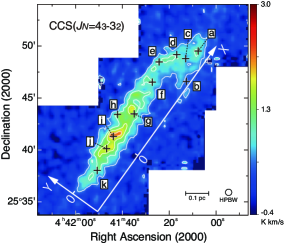
Figure 1: The CCS ($J_{N}=4_{3}-3_{2}$) intensity map integrated from 5 km s^-1 to 7 km s^-1. We set $X$ and $Y$ axes as shown in the panel. The position of the CCS peak is located at $(X,Y)=(0\arcmin,0\arcmin)$ whose equatorial coordinates are $\alpha_{\rm J2000}$=04^h41^m43.87^s and $\delta_{\rm J2000}$=+25^∘41$\arcmin$17.7$\arcsec$. Plus signs labeled “a”–“k” indicate the positions where the CCS spectra shown in Figure 2 are sampled. Positions with labels “b”, “c”, and “i” correspond to IRAS 04381+2540, the NH₃ peak position (Fehér et al., 2016), and the CCS peak position, respectively.

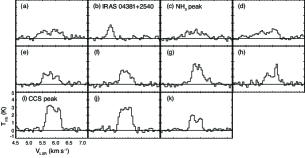
Figure 2: Panels (a)–(k) show the CCS spectra sampled at the positions “a”–“k” in Figure 1 in this order. Spectra in panels (b), (c), and (i) are observed toward IRAS 04381+2540, the NH₃ peak (Fehér et al., 2016), and the CCS peak, respectively. All of the spectra are smoothed to the 0.05 km s^-1 velocity resolution.

3 Distributions of the CCS Emission

In Figure 1, we show the intensity map of the CCS ($J_{N}=4_{3}-3_{2}$) emission integrated from 5 km s^-1 to 7 km s^-1. The TMC-1 filament has an aspect ratio of $\sim 7$ with a major axis of $\sim 20\arcmin$ and minor axes of $\sim 3\arcmin$. At a distance of 140 pc (e.g., Elias, 1978), the minor axis has a length of about 0.1 pc, comparable to the typical diameter of the Herschel filament. The TMC-1 filament detected in the CCS intensity map appears to be consistent with that of the Herschel image (Fehér et al., 2016). Hereafter, we define the $X$ and $Y$ axes of the filament as indicated in Figure 1.

The CCS emission is stronger in the southern part of the filament which appears to fragment along the major axis. The position of the strongest emission, $\alpha_{\rm J2000}$=04^h41^m43.87^s and $\delta_{\rm J2000}$=+25^∘41$\arcmin$17.7$\arcsec$, is designated by the plus sign labeled “i” in Figure 1. This position is often referred to as cyanopolyyne peak (CP). We found that the CP position is slightly shifted (by a few tens arcsecs) from the originally-reported position by earlier studies (e.g., Hirahara et al., 1992). We believe that this discrepancy comes from the different observation mode. We conducted OTF observations to obtain the map. On the other hand, previous observations were done by simple position-switch mode. Taking into account this difference, we believe that the position we identified should be more accurate.

In Figure 2, we show examples of the CCS spectra observed toward positions labeled “a”–“k” in Figure 1. Fehér et al. (2016) reported that in TMC-1 there are two velocity components at most observable in NH₃, but the CCS emission line appears complex consisting of more velocity components over the filament. In Figure 3(a), we present the position-velocity diagrams of the CCS emission along four cuts parallel to the $Y$ axis. The diagrams also imply the existence of multiple components overlapping along the line of sight. The existence of the substructures was first pointed out by Langer et al. (1995) based on the different transition data of CCS. Peng et al. (1998) observed an $8\arcmin\times 8\arcmin$ region around the CP position in the CCS($J_{N}=2_{1}-0_{1}$) and CCS($J_{N}=4_{3}-3_{2}$) emission lines with similar angular and velocity resolutions to our observations. The CCS($J_{N}=4_{3}-3_{2}$) spectra they obtained are very similar to our data in terms of the shapes, peak temperatures, and line widths. They divided the emission into three filaments by fitting the spectra with three simple Gaussian functions to find clumps along the filaments. In Appendix B, we compare our results with these earlier studies (Peng et al., 1998; Fehér et al., 2016).

Recently, we conducted a detailed analysis of the CCS and HC₃N line profiles at the CP position, taking into account the effects of radiative transfer (Dobashi et al., 2018). We found that the line profile consists of four Gaussian components with different line-of-sight velocities, which was confirmed by analyzing optically thin ($\tau\lesssim 0.17$) hyperfine lines of HC₃N. We used data having an extremely fine velocity resolution of 0.4 m s^-1 obtained with a spectrometer named PolariS (Mizuno et al., 2014), and estimated the centroid velocity of each component very accurately. Main results of our previous work related to this paper are summarized in Appendix A. For details, see Dobashi et al. (2018). The existence of the multiple components is in good agreement with our position-velocity map with a coarser velocity resolution.

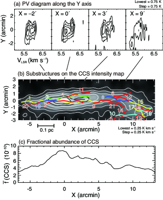
Figure 3: (a) Position-velocity (PV) diagram measured along the $Y$ axis at $X=-2\arcmin$, $0\arcmin$, $3\arcmin$, and $4\arcmin$, where $X$ and $Y$ axes are drawn in Figure 1. (b) Distributions of the subfilaments (labelled 1–21 ) shown on the CCS intensity map. (c) Fractional abundance of CCS measured as a function of $X$.

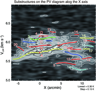
Figure 4: Distributions of the subfilaments shown on the PV diagram along the $X$ axis. The PV diagram is produced by averaging the CCS spectra over the $Y$ range $-3\arcmin<Y<3\arcmin$ at every $X$. Red circles labelled A–D at $X=0\arcmin$ denote the centroid velocities of the four components identified by Dobashi et al. (2018).

4 Velocity-Coherent Substructures

As shown in Figure 2 and Figure 3(a), the CCS spectra at several positions have multiple components along the line of sight. In the following, we identify the possible substructures in TMC-1 based on our CCS data. Hacar et al. (2013) first fitted the C¹⁸O$(J=1-0)$ spectra in L1495/B213 with $N$-component Gaussian functions and searched for velocity components having similar radial velocities in neighboring pixels using the FIVE algorithm. Following Hacar et al. (2013), we identify velocity-coherent structures in position-position-velocity space. In the case of the CCS data obtained in this work, however, it is not always easy to identify such substructures with an automatic method such as the FIVE or “clumpfind” (Williams et al., 1994) algorithms, because the emission line is not optically thin in the dense region ($\tau=1-2$) and two or more components with a small velocity difference ($0.1-0.2$ km s^-1) are aligned on the same line of sight (e.g, see Appendix A), which makes it difficult to separate them reliably. We therefore attempt to identify such structures in the position-position-velocity space by visual inspection for simplicity.

Our procedure to find the subfilaments is as follows; as shown in Figure 1, we first set the $X$ and $Y$ axes parallel and orthogonal to the elongation of TMC-1, respectively, and resampled the spectra at the 15$\arcsec$ grid along the $Y$axis by convolving the original CCS spectra with a 2 dimensional Gaussian function (FWHM$=30\arcsec$), and averaged the resulting spectra in the range $-3\arcmin<Y<3\arcmin$. We calculated the averaged spectra at every $X$ grid to produce the position-velocity (PV) diagram along the $X$ axis. Resulting PV diagram is shown in Figure 4. For a single CCS spectrum (e.g., those in Figure 2), it is not always easy to identify the individual velocity components. The PV diagram providing information of neighboring spectra is useful to find candidates of the velocity-coherent substructures which often appear as a ridge running parallel to the $X$ axis in the diagram. To investigate distributions of the substructures on the $XY$ plane, we selected a position $(X,V_{\rm LSR})$ along the ridge in the PV diagram, and calculated the CCS intensity for all of the $Y$ positions at the selected $(X,V_{\rm LSR})$ position, and plotted the peak intensity position on the $XY$ plane. We repeated this procedure for all of the positions along the noticeable ridges in the PV diagram, and regarded continuous peaks both in the PV diagram and $XY$ plane as a substructure.

In total, we found 21 CCS substructures. Their spatial and velocity distributions are delineated by the solid lines with different colors in Figures 3(b) and 4. The positions and physical quantities such as lengths, widths, and masses of the identified substructures are summarized in Table 1. The length ranges from $\sim 0.1$ pc to $\sim 0.5$ pc with a width of $0.05-0.1$ pc. Thus, the aspect ratios (the length/width ratios) are estimated to be about 0.3$-$5.7. Most of the substructures identified have aspect ratios greater than unity, indicating that they are filamentary. The substructures with aspect ratios smaller than unity are blobs or cores, instead of the filaments.

As we describe in Appendix C, there may be rather large ambiguities in our analyses which mainly arise from our method to find the substructures by visual inspection. However, most of the major substructures in TMC-1 should be detected in this survey, which provides us with important information on the structure of TMC-1. First, we found four velocity components toward the CP position, and named them A, B, C, and D in the order of their centroid velocities. In Figure 4, we indicate their locations in the PV diagram. The components apparently correspond to the substructures labeled “1”–“4”, suggesting that the velocity components A–D observed toward the CP position by our previous study are likely to be a part of the distinct substructures.

Second, we found that there is a systematic velocity gradient orthogonal to the elongation of TMC-1, which is evident in the PV diagrams in Figure 3(a). In addition, the identified substructures in the southern part of TMC-1 at $-5\arcmin\lesssim X\lesssim 3\arcmin$ in Figure 3(b) are well-aligned and concentrated around the axis of the main filament (around $Y\simeq 0\arcmin$), while those in the northern part ($5\arcmin\lesssim X\lesssim 13\arcmin$) are more widely and randomly distributed. The systematic velocity gradient seen in the southern part may infer the global infall motion in the main filament. In fact, on the basis of the detailed radiative transfer calculations with CCS and HC₃N line profiles, we proposed in our previous study (Dobashi et al., 2018) that the components A, B, C, and D having lower radial velocities in this order are aligned along the line of sight from farther side in this order, and concluded that the four components are shrinking, getting closer to one another as a whole.

Table 1: Parameters of the velocity-coherent components

	Peak Position
No.	R.A.(J2000)	Dec.(J2000)	$T_{\rm mb,max}$	$V_{\rm LSR}$	$N({\rm CCS})$	Length	${\rm Width}$	${\rm Aspect}$	Flux	Mass	Line density
			(K)	(km s-1)	(1012 cm-2)	(pc)	(pc)	${\rm Ratio}$	(K kms-1 arcmin2)	($M_{\odot}$)	($M_{\odot}$ pc-1)
1	4h41m43.0s	25∘41$\arcmin$ 9$\arcsec$	3.37	5.72	9.65	0.498	0.088	5.655	1.84	11.08	22.25
2	4h41m44.9s	25∘40$\arcmin$32$\arcsec$	2.96	5.89	8.47	0.220	0.073	3.034	0.71	3.57	16.18
3	4h41m46.1s	25∘41$\arcmin$ 2$\arcsec$	3.13	6.07	8.97	0.257	0.075	3.448	0.79	3.96	15.41
4	4h41m44.8s	25∘41$\arcmin$26$\arcsec$	2.68	6.16	7.66	0.096	0.076	1.259	0.33	1.60	16.63
5	4h41m15.4s	25∘45$\arcmin$56$\arcsec$	1.55	5.42	4.44	0.207	0.058	3.584	0.28	2.14	10.30
6	4h41m23.9s	25∘48$\arcmin$51$\arcsec$	1.63	5.81	4.68	0.105	0.117	0.904	0.27	2.34	22.24
7	4h41m38.7s	25∘42$\arcmin$55$\arcsec$	2.62	6.03	7.49	0.061	0.067	0.915	0.23	1.20	19.64
8	4h41m26.7s	25∘47$\arcmin$ 8$\arcsec$	1.97	5.71	5.64	0.176	0.101	1.737	0.41	3.43	19.50
9	4h41m30.4s	25∘44$\arcmin$40$\arcsec$	2.99	5.91	8.56	0.199	0.092	2.160	0.55	4.05	20.34
10	4h41m15.0s	25∘46$\arcmin$29$\arcsec$	2.05	5.32	5.86	0.146	0.071	2.046	0.26	2.27	15.57
11	4h41m39.1s	25∘44$\arcmin$31$\arcsec$	1.09	6.26	3.13	0.052	0.110	0.468	0.10	0.52	10.13
12	4h41m22.8s	25∘48$\arcmin$21$\arcsec$	1.53	5.55	4.37	0.089	0.102	0.874	0.18	1.54	17.27
13	4h41m 7.9s	25∘48$\arcmin$43$\arcsec$	1.30	5.57	3.73	0.170	0.135	1.254	0.23	2.07	12.21
14	4h41m14.5s	25∘47$\arcmin$56$\arcsec$	0.71	6.20	2.03	0.045	0.155	0.290	0.07	0.55	12.27
15	4h41m12.0s	25∘49$\arcmin$60$\arcsec$	1.38	6.11	3.94	0.140	0.095	1.483	0.27	2.52	17.95
16	4h41m 9.3s	25∘49$\arcmin$34$\arcsec$	1.30	5.92	3.71	0.079	0.061	1.296	0.11	1.03	13.01
17	4h41m12.8s	25∘48$\arcmin$54$\arcsec$	1.01	5.82	2.89	0.088	0.141	0.625	0.11	0.96	10.94
18	4h41m 8.0s	25∘49$\arcmin$58$\arcsec$	1.43	6.03	4.09	0.075	0.079	0.955	0.13	1.32	17.53
19	4h41m48.4s	25∘39$\arcmin$52$\arcsec$	2.66	5.99	7.60	0.125	0.064	1.940	0.32	1.91	15.36
20	4h41m51.8s	25∘37$\arcmin$57$\arcsec$	1.76	5.77	5.05	0.065	0.079	0.825	0.13	1.05	16.13
21	4h41m26.1s	25∘46$\arcmin$26$\arcsec$	1.56	5.84	4.48	0.053	0.120	0.436	0.16	1.40	26.66

Note. — Coordinates, $T_{\rm mb,max}$ the maximum brightness temperature, $V_{\rm LSR}$ the centroid velocity, $N($CCS$)$ the column density are measured at the intensity peak position of substructures.

5 Masses of the substructures

To study the dynamical states of the substructures, we derived their masses using the CCS data. The excitation temperatures of the CCS and HC₃N lines are reported to be $T_{\rm ex}\simeq 6-12$ K at the CP position (Dobashi et al., 2018), but it should vary slightly over TMC-1. For simplicity, we assumed a constant excitation temperature of $T_{\rm ex}=10$ K and an optically thin case in this paper. The masses derived in this section only weakly depend on the assumed $T_{\rm ex}$, and they would vary by $\sim 12$ $\%$ at most in the range $T_{\rm ex}=5-15$ K.

First, we estimated the fractional abundance of CCS relative to H₂, $f{\rm(CCS)}$. For the observed positions where the CCS emission is significantly detected with velocity-integrated intensity greater than $I_{\rm CCS}\geqq 0.2$ K km s^-1, we calculated the column density of CCS in a standard way (e.g., Shimoikura et al., 2018a) at each observed position as

$$N{\rm(CCS)}=C_{0}I_{\rm CCS}\$$ (1)

where $C_{0}$ is a function of $T_{\rm ex}$ and is $1.683\times 10^{13}$ (K km s^-1)^-1 cm^-2 for $T_{\rm ex}=10$ K. We then estimated $f{\rm(CCS)}$ as $f{\rm(CCS)}=N{\rm(CCS)}/N{\rm(H_{2})}$ where $N$(H₂) is the column density of hydrogen molecules calculated in a standard way (e.g., Shimoikura et al., 2013) using the C¹⁸O ($J=1-0$) data available at the Nobeyama 45-m data archive (e.g., see Dobashi et al., 2018). The fractional abundance of C¹⁸O is assumed to be $f$(C¹⁸O$)=1.7\times 10^{-7}$ (Frerking et al., 1982). Though there is a clear tendency that the derived $f$(CCS) is smaller in the northern part of TMC-1, it varies rather largely from pixel to pixel. We therefore smoothed $f$(CCS) along the $Y$ axis at every $X$ grid to derive the mean CCS fractional abundance $\bar{f}$(CCS) as a function of $X$, which we actually used to calculate the molecular masses of the substructures. As displayed in Figure 3(c), $\bar{f}$(CCS) varies from $2\times 10^{-10}$ to $9\times 10^{-10}$ within the elongation of TMC-1.

Next, we produced the velocity-integrated CCS intensity map $I_{\rm CCS}^{\rm sub}$ for each substructure. Assuming that the substructures have a constant radial velocity along the $Y$ axis, we extracted a value of the brightness temperature $T_{\rm mb}$(CCS) for every $Y$ grid at the velocity of the substructures $V_{\rm LSR}$ measured at each $X$ grid, and we made a map of the brightness temperature of the substructure $T_{\rm mb}^{\rm sub}$($X,Y$). We further estimated the velocity-integrated intensity maps $I_{\rm CCS}^{\rm sub}$ as $I_{\rm CCS}^{\rm sub}=T_{\rm mb}^{\rm sub}\Delta V^{\rm sub}$ where $\Delta V^{\rm sub}$ is the FWHM line width of the substructures. The true $\Delta V^{\rm sub}$ should be different from substructure to substructure and should also vary depending on the positions ($X,Y$). It is however very difficult to quantify $\Delta V^{\rm sub}$, and we therefore adopted the mean value $\Delta V^{\rm sub}=0.17$ km s^-1 of the four velocity components A–D observed at the CP position (Dobashi et al., 2018). We derived distributions of $N$(CCS) by substituting $I_{\rm CCS}^{\rm sub}$ for $I_{\rm CCS}$ in Equation (1), and derived the total molecular mass of each substructure by applying $\bar{f}$(CCS) and assuming a distance of 140 pc (e.g., Elias, 1978). The derived masses are summarized in Table 1. Note that the masses in the table would increase by $\sim 10$ $\%$, if we adopt a distance of $\sim 148$ pc reported by Loinard et al. (2007). In the table, flux denotes the total $I_{\rm CCS}^{\rm sub}$ summed over the substructures, and width denotes the mean FWMH width of $I_{\rm CCS}^{\rm sub}$ along the $Y$ axis. Aspect ratio is the ratio of length to width, and line density is defined to be the mass divided by the length. The total and mean masses of the 21 substructures in Table 1 are $\sim 50$ $M_{\odot}$ and $\sim 2.4$ $M_{\odot}$, respectively. Total molecular mass of the entire TMC-1 filament measured in C¹⁸O is $\sim 200$ $M_{\odot}$ (see Figure 8b of Dobashi et al., 2018), and thus $\sim 25$ $\%$ of the molecular mass is contained in the substructures.

The dynamical state of an isothermal filamentary cloud is determined by the line density, which is given as

$$m={2c_{s}^{2}\over G}\simeq 464\left({c_{s}\over{\rm km\ s^{-1}}}\right)^{2}M_{\odot}{\rm pc^{-1}}\ ,$$ (2)

where $c_{s}$ and $G$ are the isothernal sound speed and gravitational constant, respectively (Stodólkiewicz, 1963; Ostriker, 1964). The dust temperature in TMC-1 is measured to be $\sim$ 11 K on the basis of the Herschel observations (Fehér et al., 2016). If we adopt the isothermal sound speed at $T\simeq 10$ K ($c_{s}=0.2$ km s^-1), the critical line density for the dynamical equilibrium is estimated to be 17 $M_{\odot}$ pc^-1. Though our mass estimates based on the CCS data are rather coarse, most of the identified substructures have masses comparable to the critical value, and thus we believe that they should be close to the dynamical equilibrium. These nearly-equilibrium structures seem to have similar dynamical properties of the fibers identified by Hacar et al. (2017). It is also interesting to note that Peng et al. (1998) identified $45$ small clumps in CCS along the filamentary structures around the CP position, and they suggested that most of the clumps are gravitationally stable or unbound, though the optical depth of the emission line and the related radiative transfer were not taken into account in their analyses.

6 Discussion

A bundle of aligned substructures as seen in the southern part of TMC-1 can sometimes be recognized in numerical simulations to study the formation and evolution of dense filaments, although it remains uncertain whether the velocity-coherent substructures we found are the same as those found in the numerical simulations. For example, in the simulations performed by Dobashi et al. (2014) and Matsumoto et al. (2015), filaments naturally form in dense clumps mainly by turbulence, and they often consist of smaller substructures. Similar results are reported by Moeckel & Burkert (2015). (see also Zamora-Avilés et al. (2017) and Smith et al. (2016)). The substructures are gravitationally stable and scarcely collapse spontaneously by themselves, but when they happen to cross (or collide against) each other, they can soon form stars due to the increase of density at the intersections (e.g., see Figure 19 of Dobashi et al., 2014). Similar effects of filament-filament collisions on star formation have been reported also in other star-forming regions (e.g., Nakamura et al., 2014). We imagine that TMC-1 consists of such smaller, gravitationally stable substructures, and as predicted by the simulations, it would soon form stars when the internal substructures happen to cross each other.

The origin of the velocity-coherent substructures identified here and their role in the star formation process are still uncertain. They might be created by local cloud turbulence, as predicted by the numerical simulations. Recently, we found that the substructures Nos. 1 and 4 are infalling with a speed of $\sim$ 0.4 km s^-1 toward the center (Dobashi et al., 2018) at the CP position. If the TMC-1 filament is infalling toward the major axis, such a global infall motion may create local denser parts (e.g., substructures Nos.1 and 4) generated by shock. Thus, there is a possibility that we just see such local peaks temporally created in the main filament. To fully understand the origin and role of the substructures in star formation process, further investigation on the kinematics and internal structures of Herschel filaments and substructures would be needed.

7 Conclusions

We have observed the Taurus Molecular Cloud 1 (TMC-1) in the CCS($J_{N}=4_{3}-3_{2}$) emission line at 45 GHz using the Nobeyama 45-m telescope. We found that TMC-1 has a filamentary morphology with a diameter of $\sim 0.1$ pc and a length of $\sim 0.5$ pc. We identified 21 velocity-coherent substructures in TMC-1 by eye, and found that the substructures have a mass close to the critical values for the gravitational equilibrium.

Appendix A Four velocity components at the cyanopolyyne peak

Based on sensitive CCS and HC₃N spectral data, we recently identified four velocity components at the CP position, and reported the results in another article (Dobashi et al., 2018). In the following, we briefly review the methods and results of our previous work.

We observed the CP position with the CCS($J_{N}=4_{3}-3_{2}$) and HC₃N($J=5-4$) lines simultaneously using the Z45 receiver installed on the Nobeyama 45-m telescope. We used a spectrometer named PolariS (Mizuno et al., 2014) which provided an extremely high frequency resolution of 61 Hz corresponding to the $\sim 0.4$ m s^-1 velocity resolution. Total integration of $\sim 30$ hr suppressed the rms noise of the spectral data to $\Delta T_{\rm a}^{*}\simeq 40$ mK for the $\sim 0.4$ m s^-1 velocity resolution. Resulting spectra related to this work are displayed in Figure 5(a) and (b).

The HC₃N($J=5-4$) line consists of five hyperfine structures ($F=5-5$, $4-3$, $5-4$, $6-5$, and $4-4$). Among these, the $F=4-4$ and $5-5$ lines have intrinsically the same intensity, and are well separated in frequency from the other hyperfine lines. Therefore they can be averaged directly to reduce noise. The spectrum in Figure 5(a) is the average spectrum of the $F=4-4$ and $5-5$ lines. The $F=4-4$ and $5-5$ lines are generally optically thin. In fact, the maximum optical depth at the CP position is $\tau\lesssim 0.17$ (for details, see Dobashi et al., 2018). Therefore, under the assumption of the Local Thermodynamic Equilibrium (LTE), the spectrum in Figure 5(a) can be approximated by a simple Gaussian function with $N$ velocity components. We fitted the average HC₃N spectrum with a Gaussian function with $N$ velocity components leaving the centroid velocity, peak intensity, and line width of each component as free parameters. We calculated the reduced $\chi^{2}$ (hereafter, $\chi^{2}_{r}$) of the residual of the best fit for increasing $N$($=1$, $2$, $3$, and so on). We found that $\chi^{2}_{r}$ rapidly decreases up to $N=4$ ($\chi^{2}_{r}=1.0016$), and also that $\chi^{2}_{r}$ doesn’t change significantly for larger $N(\geqq 5)$. This indicates that the spectrum consists of $N=4$ distinct velocity components. We named the four components A, B, C, and D in the order of increasing centroid velocities. These components are shown by the solid lines with different colors in Figure 5(a). The fitted centroid velocities are given in Figure 5(c).

We assumed that the CCS line consists of the same velocity components having the same centroid velocities as those found in the HC₃N line, because the CCS and HC₃N lines should trace similar density regions ($n_{\rm H_{2}}=10^{4-5}$ cm^-3). We fitted the observed CCS spectrum with a Gaussian function which consists of $N=4$ velocity components with the fixed centroid velocities, leaving the line width, excitation temperature, and optical depth of each component as free parameters. Because the CCS line is not optically thin, radiative transfer should be taken into account in the fitting process. We looked for the parameters best fitting the observed CCS spectrum for all of the permutations ($N!=4!=24$) of the relative positions for the four velocity components along the line-of-sight, and calculated $\chi^{2}_{r}$ of the residual of the best fit for each permutation. As a result, we found that the minimum $\chi^{2}_{r}$ ($=1.063$) can be found when the components A, B, C, and D are lying from far side to near side from the observer in this order as illustrated in Figure 5(c). In Figure 5(b), contributions of the four components to the observed CCS spectrum are shown by the lines with different colors. Note that the contribution of each component cannot be expressed by a simple Gaussian function, not only because they are not optically thin, but also because they are partially absorbed by the other component(s) in the foreground. In the same way as for the CCS line, we analyzed the other hyperfine lines of HC₃N (i.e., $F=4-3$, $5-4$, $6-5$) which are blended and optically thicker, and obtained the same results as for the CCS line (see Figure 6 of Dobashi et al., 2018).

In addition to the above results, we pointed out a possibility that the centroid velocities and the relative locations of the components A–D along the line-of-sight illustrated in Figure 5(c) may represent the global infalling motion of TMC-1.

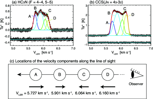
Figure 5: (a) The averaged spectrum of the two hyperfine transitions $F=4-4$ and $5-5$ of the HC₃N($J=5-4$) line, and (b) the CCS($J_{N}=4_{3}-3_{2}$) line observed toward the CP peak with the PolariS spectrometer. The original velocity resolution is 0.4 m s^-1, and it is smoothed to 0.8 m s^-1 in the panels. Four velocity components labeled “A”–“D” identified in the spectra are shown by the lines with different colors, and their sums best fitting the observed spectra are shown by the red lines. Residuals offset by $-0.3$ K and $-0.9$ K in panels (a) and (b), respectively, are also shown. The spectra are shown in units of the antenna temperature $T_{\rm a}^{*}$ related to the brightness temperature as $T_{\rm mb}={\eta}^{-1}T_{\rm a}^{*}$ where $\eta$ ($=0.7$ at 45 GHz) is the main beam efficiency of the 45-m telescope. (c) Inferred relative locations of the four velocity components along the line of sight. The figures are taken from Dobashi et al. (2018).

Appendix B Comparison with earlier studies

We compare our results with two earlier studies to investigate the substructures of TMC-1. One is the CCS observations around the CP position performed by Peng et al. (1998). They divided the CCS emission into three filamentary structures having typical radial velocities of $5.7$, $5.9$, and $6.1$ km s^-1 by fitting the spectra with a simple Gaussian function with three components at most (see their Figure 2). The first two components mainly correspond to our substructures “1” and “2”, respectively, and the third component is a mixture of our substructures “3” and “4”. A few other substructures identified in our work around the CP position (e.g., “19” and “20”) are not recognized or are merged to one of the three components in their work, because of their assumption of the three components at most over the $8\arcmin\times 8\arcmin$ region they observed. Except for these points, the results of Peng et al. (1998) are consistent with our results.

The other is the recent work by Fehér et al. (2016) who observed the entire TMC-1 filament in NH₃. In their NH₃ data, there can be seen a clear velocity gradient orthogonal to the axis of the main filament (see Figure 5 of Fehér et al., 2016), which is consistent with what we see in Figure 3a. They suggested existence of four filamentary substructures which they call “F1”, “F2”, “F3”, and “F4”. The lengths ($\sim 0.5$ pc) and radius ($0.1-0.2$ pc) of their substructures are similar to our substructures, but their distributions on the plane of the sky appear very different. This is because they fitted the spectra only with two velocity components at most and classified the components using “$k$-means clustering method”. Their F1–F4 are apparently mixtures of our substructures “1”–“21”, but it is difficult to identify their correspondence clearly. Coincidence of their and our substructures on the plane of the sky can be summarized as follows; their F1 contains our substructures “12”, “15”, and “21”, and F2 contains “11”. F3 contains “5”, “10”, “13”, and “14”, and F4 contains “1”–“4”, “7”, “19”, and “20”. Our “6” is shared by F1 and F2, and “9” is shared by F2 and F3. Finally, “16”, “17”, and “18” are shared by F1 and F3.

Major differences between our results and those of the earlier studies arise from the assumptions on the number of velocity components. For example, Peng et al. (1998) and Fehér et al. (2016) assume three and two velocity components around the CP position, while we found four components toward the position, which agrees with the detailed analyses in our previous work (Dobashi et al., 2018) as stated in Section 4.

Appendix C Uncertainties of our analyses

We describe caveats and ambiguities in our analyses. We first describe possible errors arising from our method to find substructures. We identified 21 substructures which should trace most of the major substructures in TMC-1. However, there may be some more substructures which escaped detection, because we searched them by visual inspection. In addition, our method to find substructures is apparently insufficient to identify and quantify filaments extending parallel to the $Y$ axis, and there might be some filamentary substructures extending nearly orthogonal to the $X$ axis. For example, candidates of such features can be seen at $X\simeq-2\arcmin$ and $X\simeq 6\arcmin$ in Figure 3(b) which we did not analyze in this paper. In addition, we can identify only one of two (or more) filaments having the same $V_{\rm LSR}$ and running parallel to the $X$ axis, because the method allows us to pick up only one $Y$ position for a given ($X$,$V_{\rm LSR}$) position. This is also a source of the incomplete sampling. The lengths of the substructures in Table 1 should be the lower limits to the actual lengths because of this shortcoming of the method.

Finally, we describe errors in our mass estimate of the substructures. The estimate is basically based on the C¹⁸O data, and therefore its accuracy depends on the ambiguity of the assumed fractional abundance of C¹⁸O. The assumed fractional abundance ($1.7\times 10^{-7}$) originally have an ambiguity of a factor of $\sim 3$ (Frerking et al., 1982). In addition, the C¹⁸O molecule is known to be adsorbed onto dust in dense regions (e.g., Bergin et al., 2002). In fact, the intensity of the C¹⁸O spectrum at the CP peak is about one half of what we would expect without adsorption (see Figure 9 of Dobashi et al., 2018), and therefore the derived total mass of the subscrutcures can be underestimated by a factor of $\sim 2$ by this effect. The assumed constant line width ($\Delta V^{\rm sub}=0.17$ km s^-1) is also a source of errors, because it is actually varying by a factor of $\sim 2$ depending on the velocity components even at the CP peak (see $\sigma^{i}$ in Table 3 of Dobashi et al., 2018). These errors arising from the assumptions on the fractional abundance and the line width may result in the total ambiguity of a factor of $\sqrt{3^{2}+2^{2}+2^{2}}\simeq 4$ in our mass estimate. There must be some other sources of errors not mentioned in the above, and thus the factor $\sim 4$ should be the minimum estimate of the total uncertainty in the derived mass of the subsctructures.

References

- André et al. (2014) André, P., Di Francesco, J., Ward-Thompson, D., et al. 2014, Protostars and Planets VI, 27
- Bergin et al. (2002) Bergin, E. A., Alves, J., Huard, T., & Lada, C. J. 2002, ApJ, 570, L101
- Dobashi et al. (2014) Dobashi, K., Matsumoto, T., Shimoikura, T., et al. 2014, ApJ, 797, 58
- Dobashi et al. (2018) Dobashi, K., Shimoikura, T., Nakamura, F., et al. 2018, ApJ, 864, 82
- Elias (1978) Elias, J. H. 1978, ApJ, 224, 857
- Fehér et al. (2016) Fehér, O., Tóth, L. V., Ward-Thompson, D., et al. 2016, A&A, 590, A75
- Frerking et al. (1982) Frerking, M. A., Langer, W. D., & Wilson, R. W. 1982, ApJ, 262, 590
- Hacar et al. (2017) Hacar, A., Tafalla, M., & Alves, J. 2017, A&A, 606, A123
- Hacar et al. (2013) Hacar, A., Tafalla, M., Kauffmann, J., & Kovács, A. 2013, A&A, 554, A55
- Hirahara et al. (1992) Hirahara, Y., Suzuki, H., Yamamoto, S., et al. 1992, ApJ, 394, 539
- Hirota et al. (2009) Hirota, T., Ohishi, M., & Yamamoto, S. 2009, ApJ, 699, 585
- Langer et al. (1995) Langer, W. D., Velusamy, T., Kuiper, T. B. H., et al. 1995, ApJ, 453, 293
- Loinard et al. (2007) Loinard, L., Torres, R. M., Mioduszewski, A. J., et al. 2007, ApJ, 671, 546
- Matsumoto et al. (2015) Matsumoto, T., Dobashi, K., & Shimoikura, T. 2015, ApJ, 801, 77
- Mizuno et al. (2014) Mizuno, I., Kameno, S., Kano, A., et al. 2014, Journal of Astronomical Instrumentation, 3, 1450010
- Moeckel & Burkert (2015) Moeckel, N., & Burkert, A. 2015, ApJ, 807, 67
- Nakamura et al. (2012) Nakamura, F., Takakuwa, S., & Kawabe, R. 2012, ApJ, 758, L25
- Nakamura et al. (2014) Nakamura, F., Sugitani, K., Tanaka, T., et al. 2014, ApJ, 791, L23
- Nakamura et al. (2015) Nakamura, F., Ogawa, H., Yonekura, Y., et al. 2015, PASJ, 67, 117
- Ostriker (1964) Ostriker, J. 1964, ApJ, 140, 1056
- Peng et al. (1998) Peng, R., Langer, W. D., Velusamy, T., Kuiper, T. B. H., & Levin S. 1998, ApJ, 497, 842
- Ruaud et al. (2016) Ruaud, M., Wakelam, V., & Hersant, F. 2016, MNRAS, 459, 3756
- Shimoikura et al. (2015) Shimoikura, T., Dobashi, K., Nakamura, F., et al. 2015, ApJ, 806, 201
- Shimoikura et al. (2018a) Shimoikura, T., Dobashi, K., Nakamura, F., Matsumoto, T., & Hirota, T. 2018a, ApJ, 855, 45
- Shimoikura et al. (2018b) Shimoikura, T., Dobashi, K., Nakamura, F., Shimajiri, Y., & Sugitani, K. 2018b, PASJ, arXiv:1809.09855
- Shimoikura et al. (2012) Shimoikura, T., Dobashi, K., Sakurai, T., et al. 2012, ApJ, 745, 195
- Shimoikura et al. (2013) Shimoikura, T., Dobashi, K., Saito, H., et al. 2013, ApJ, 768, 72
- Smith et al. (2016) Smith, R. J., Glover, S. C. O., Klessen, R. S., & Fuller, G. A. 2016, MNRAS, 455, 3640
- Stodólkiewicz (1963) Stodólkiewicz, J. S. 1963, Acta Astron., 13, 30
- Suzuki et al. (1992) Suzuki, H., Yamamoto, S., Ohishi, M., et al. 1992, ApJ, 392, 551
- Taniguchi et al. (2018a) Taniguchi, K., Miyamoto, Y., Saito, M., et al. 2018a, ApJ, 866, 32
- Taniguchi et al. (2017a) Taniguchi, K., Ozeki, H., & Saito, M. 2017a, ApJ, 846, 46
- Taniguchi et al. (2016a) Taniguchi, K., Ozeki, H., Saito, M., et al. 2016a, ApJ, 817, 147
- Taniguchi & Saito (2017) Taniguchi, K., & Saito, M. 2017, PASJ, 69, L7
- Taniguchi et al. (2016b) Taniguchi, K., Saito, M., & Ozeki, H. 2016b, ApJ, 830, 106
- Taniguchi et al. (2018b) Taniguchi, K., Saito, M., Sridharan, T. K., & Minamidani, T. 2018b, ApJ, 854, 133
- Taniguchi et al. (2017b) Taniguchi, K., Saito, M., Hirota, T., et al. 2017b, ApJ, 844, 68
- Taniguchi et al. (2018c) Taniguchi, K., Saito, M., Majumdar, L., et al. 2018c, ApJ, 866, 150
- Williams et al. (1994) Williams, J. P., de Geus, E. J., & Blitz, L. 1994, ApJ, 428, 693
- Wolkovitch et al. (1997) Wolkovitch, D., Langer, W. D., Goldsmith, P. F., & Heyer, M. 1997, ApJ, 477, 241
- Zamora-Avilés et al. (2017) Zamora-Avilés, M., Ballesteros-Paredes, J., & Hartmann, L. W. 2017, MNRAS, 472, 647