Higgs Parity Grand Unification
Abstract
The vanishing of the Higgs quartic coupling of the Standard Model at high energies may be explained by spontaneous breaking of Higgs Parity. Taking Higgs Parity to originate from the Left-Right symmetry of the gauge group, leads to a new scheme for precision gauge coupling unification that is consistent with proton decay. We compute the relevant running of couplings and threshold corrections to allow a precise correlation among Standard Model parameters. The scheme has a built-in solution for obtaining a realistic value for , which further improves the precision from gauge coupling unification, allowing the QCD coupling constant to be predicted to the level of 1% or, alternatively, the top quark mass to 0.2%. Future measurements of these parameters may significantly constrain the detailed structure of the theory. We also study an embedding of quark and lepton masses, showing how large neutrino mixing is compatible with small quark mixing, and predict a normal neutrino mass hierarchy. The strong CP problem may be explained by combining Higgs Parity with space-time parity.
I Introduction
The discoveries of a perturbative Higgs boson at the Large Hadron Collider Aad et al. (2012); Chatrchyan et al. (2012) and no new states beyond the Standard Model (SM) Aaboud et al. (2018); Sirunyan et al. (2018) suggest that the SM may be the correct effective theory of particle physics up to a scale orders of magnitude larger than the weak scale, a possibility largely ignored before the Large Hadron Collider. In such a scenario, progress in particle physics will depend on both precision measurements of SM parameters, as well as searches for rare processes, for example those violating baryon number, lepton numbers and CP.
Precision measurements can probe particle physics to extremely high energies. In 1974 Georgi, Quinn and Weinberg proposed that measurements of the three gauge couplings of the SM, , could test whether the three gauge forces of nature are unified into a single grand unified gauge force with coupling strength, , at some very high unified mass scale Georgi et al. (1974). The two fundamental UV parameters lead to a correlation among the three measured gauge couplings: . After decades of measurements, this correlation is at best a first order approximation, requiring very large threshold corrections from the unified scale to force the low energy gauge couplings to meet and to make sufficiently large to be consistent with the experimental limit on the proton lifetime. Similarly, the simplest Georgi and Glashow (1974) prediction for fermion masses, the ratio Chanowitz et al. (1977), is also at best a first order result, requiring large corrections. Nevertheless, unification is a bold and exciting vision that explains the gauge quantum numbers of the quarks and leptons, including charge quantization, and can be probed via precision measurements of SM parameters at low energy.
Precision measurements of the weak mixing angle at LEP Decamp et al. (1990) supported supersymmetric unification. Triggering the weak scale from supersymmetry breaking, , gave a successful correlation of the low energy gauge couplings via Dimopoulos et al. (1981); Dimopoulos and Georgi (1981); Sakai (1981); Ibanez and Ross (1981); Einhorn and Jones (1982); Marciano and Senjanovic (1982). While theories with a sufficiently long proton lifetime were easily constructed, the absence of superpartners at the Large Hadron Collider now makes it difficult to identify with the weak scale, weakening the theoretical basis for this correlation.
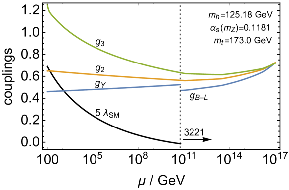
With a 125 GeV Higgs and the SM valid to sufficiently high energies, the Higgs quartic coupling of the SM passes through zero at a scale of order GeV Buttazzo et al. (2013), as shown in Fig. 1. This very striking behavior suggests that new physics lies at the scale where the Higgs quartic coupling vanishes, and that this new physics should explain the vanishing quartic via a new symmetry. One possibility is that the new symmetry is supersymmetry; although the vanishing of the quartic is not guaranteed, it does occur in a large portion of parameter space Hall and Nomura (2014); Hall et al. (2014a). We have recently introduced another possibility, “Higgs Parity” Hall and Harigaya (2018), that interchanges the weak gauge group (and SM Higgs, ) with a partner gauge group (and partner Higgs, )
| (1) |
where the quantum numbers of and refer to . Spontaneously breaking by leads to the Higgs being a Nambu-Goldstone boson with at tree-level. Depending on the implementation, this can also solve the strong CP problem Hall and Harigaya (2018) and lead to interesting dark matter candidates Dunsky et al. (2019).

In this paper we identify as the subgroup of the unified gauge group Georgi (1975); Fritzsch and Minkowski (1975), so that is identified as the scale of parity breaking. In unification, an intermediate scale of symmetry breaking introduces an extra free parameter so that the correlation of from gauge coupling unification is lost. However, in theories with Higgs Parity, is predicted from the Higgs mass so that a correlation is recovered, as illustrated in Fig. 1; three parameters of the unified theory yield a correlation among four measured observables, . In fact, the uncertainty in this correlation is dominated by the top quark Yukawa coupling via renormalization of the quartic coupling, so that in Higgs Parity Unification four UV parameters of the theory yield a correlation among five low energy observables Hall and Harigaya (2018)
| (2) |
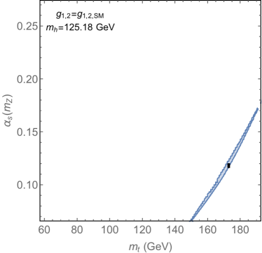
Fixing three of the observables to their central measured values, allows a projection of this correlation into a two-dimensional subspace, as shown for and in the left and right panels of Fig. 2. The blue shaded region allows for threshold corrections at the unification scale with (see Eq. (19)). The black rectangles show the observed SM values. In Figs. 1 and 2 the gauge group above is .
The organization of the paper is as follows. Secs. II and III summarize the essence of Higgs Parity unification. In Sec. II, we review how Higgs Parity explains the vanishing of the SM Higgs quartic at a high scale. Sec. III discusses the embedding of Higgs Parity into unified theories and how gauge coupling unification is tied to the vanishing quartic coupling. Secs. IV-VII analyze the framework in more detail. Sec. IV examines the running of gauge couplings between electroweak and unified scales, including threshold corrections at the unification scale, and derives the Higgs Parity symmetry breaking scale required for successful precision gauge coupling unification. The generation of the SM fermion masses is discussed in Sec. V. We show how the mass ratio and the structure of neutrino masses arise from an unified theory. In Sec. VI, we derive the threshold corrections to the SM Higgs quartic coupling at the Higgs Parity symmetry breaking scale, and show the relation between and the Parity symmetry breaking scale. Finally, the prediction for from the precise coupling unification is given in Sec. VII.
II Higgs Quartic Coupling and Higgs Parity
In this section we review the relation between the nearly vanishing SM Higgs quartic coupling at high energy scales and the Higgs Parity symmetry breaking scale introduced in Hall and Harigaya (2018). Consider a symmetry which exchanges the SM gauge symmetry with a new gauge interaction , as well as the SM Higgs field with its partner . Here the brackets show the quantum numbers. We refer to this symmetry as Higgs Parity.
Well below the cut off scale, the following renormalizable scalar potential dominates the dynamics of and ,
| (3) |
We assume and , the electroweak scale. Higgs Parity is spontaneously broken by the vacuum expectation value (VEV) , with . After integrating out , the low energy effective potential of is
| (4) |
To obtain the hierarchy , it is necessary to take a very small value of , leading to a small value of the SM Higgs quartic coupling . This is the boundary condition on at the renormalization scale . Renormalization group running from the top quark yukawa makes around the electroweak scale. From the IR perspective, the scale is identified with the energy scale around which the SM Higgs quartic coupling vanishes. Threshold corrections to as well as a precise prediction for are presented in Sec. VI.
In this paper, we identify Higgs Parity with the Left-Right symmetry which can be embedded into grand unification. As we illustrated in the introduction and will elaborate in Sec. VII, this identification leads to a non-trivial scheme for precise gauge coupling unification.
III Grand Unification and the Strong CP Problem
III.1 Left-Right symmetry as Higgs Parity
Let us first embed Higgs Parity into the Left-Right symmetry where is identified with . The gauge symmetry above the scale is or , which we refer to as or for short. 422 is the Pati-Salam gauge group Pati and Salam (1974), and is a subgroup of . The gauge quantum numbers of SM fermions, and are shown in Table 1. The Left-Right symmetry, which we denote as , is
| (5) |
and includes Higgs Parity. This results in the Higgs having gauge quantum numbers identical to leptons, which is not standard for Left-Right theories Beg and Tsao (1978); Mohapatra and Senjanovic (1978); Kibble et al. (1982); Chang et al. (1984a, b); Lazarides and Shafi (1985). The 3221 or 422 gauge groups are broken down to the group by the VEV of .
We may also combine Left-Right symmetry with another discrete symmetry; the most interesting option being space-time parity,
| (6) |
which we denote as . As we will see, the strong CP problem may then be solved.
| 1 | 1 | 1 | 1 | |||
III.2 Yukawa couplings and the strong CP problem
The gauge charges in Table 1 forbid renormalizable yukawa couplings. Instead, the SM fermion masses arise from the mixing of with extra massive fermions via yukawa couplings and masses of the form
| (7) |
After obtains a VEV, mixes with . A linear combination of them remains massless and has the yukawa coupling . If the mass of is much larger than , we may integrate out to obtain a dimension-five operator , which yields a yukawa coupling .
The strong CP problem can be solved by combining Left-Right symmetry with space-time parity, as the symmetry forbids the term and constrains the determinant of the quark mass matrix Beg and Tsao (1978); Mohapatra and Senjanovic (1978). See Refs. Barr et al. (1991); Kuchimanchi (1996); Mohapatra and Rasin (1996a, b); Mohapatra et al. (1997); Kuchimanchi (2010); D’Agnolo and Hook (2016); Albaid et al. (2015); Babu et al. (2019); Mimura et al. (2019) for studies on Left-Right symmetric solutions to the strong CP problem. Refs. Babu and Mohapatra (1989, 1990) propose a model with a structure for yukawa couplings similar to ours and show that the strong CP problem is actually solved since and is Hermitian. They obtain the hierarchy by softly breaking the Left-Right symmetry with space-time parity. In out setup the symmetry, which we call Higgs Parity, is spontaneously broken without soft breaking, predicting a vanishing . Spontaneous breaking of parity generates a phase in the determinant of the quark mass matrix via two-loop quantum corrections Hall and Harigaya (2018). Assuming that the couplings are , the corrections are safely below the current limit from the neutron electric dipole moment, but in the range that can be probed by planned experiments. The model of flavor presented in Sec. V does not obey this assumption, and the corrections may be larger.
III.3 unification
The 3221 and 422 theories can both be embedded into grand unified theories. The gauge charges of the SM fermions, and are shown in Table 1. The SM fermions are unified into three s, and the Higgs fields and are also embedded into a .
The symmetry breaking pattern is
The theory has three UV parameters relevant for gauge coupling unification: the gauge coupling, the symmetry breaking scale, and the LR symmetry breaking scale . As there are also three SM gauge coupling constants, it is not surprising that one can typically find a set of the three UV parameters that allow coupling unification. However, as we have shown, the LR symmetry breaking scale is not a free parameter when it is linked to Higgs Parity breaking, but is determined by the running of the SM Higgs quartic coupling. In this case, it would be significant if coupling unification were successful. In Fig. 1, we fix the scale using the central values of the Higgs mass, top quark mass and QCD coupling shown in the figure, and solve the RGE equations assuming the 3221 theory. Remarkably, gauge coupling unification occurs, and at a scale consistent with the proton lifetime.
III.4 Degree of fine-tuning
We comment on the fine-tuning of parameters in the Higgs potential (3) required for symmetry breaking. First, must be fine-tuned by an amount , so that the Higgs Parity breaking scale is much less than the cutoff scale , which must be larger than the unified scale . Secondly, must be fine-tuned by an amount to obtain the electroweak scale from the scale . The total fine-tuning with Higgs Parity is the product
| (8) |
which is independent of . This is because a smaller requires more fine-tuning in , but this is compensated by less fine-tuning in to obtain the electroweak scale from the scale . It is important to note that Higgs Parity, , ensures that the mass terms for and in (3) are identical, so that the single fine-tune by protects both scalars to the scale . Given that the SM Higgs must be protected for electroweak symmetry breaking, there is no additional cost to protect : the smallness of the scale requires no unnaturalness beyond that already needed for the weak scale. The total fine-tuning of the theory is nothing but the electroweak fine-tuning, which may be explained by environmental selection Agrawal et al. (1998); Hall et al. (2014b).
This is in contrast to the usual unification with an intermediate scale . A smaller intermediate scale does not reduce the fine-tuning to obtain the electroweak scale, and hence the total fine-tuning is
| (9) |
This extra fine-tuning cannot be explained by environmental selection of the electroweak scale, and requires an additional explanation.
IV Gauge Coupling Unification and Parity Breaking Scale
We assume an gauge symmetry at a high energy scale, broken to or at the unification scale. These are then broken to the SM gauge group by the VEV of . One possibility is that Higgs Parity is , a subgroup of that interchanges and . In this case, the symmetry breaking chain and the required Higgs fields are
| (10) | ||||
| (11) |
To solve the strong CP problem, the symmetry to begin with is . This symmetry is broken by the VEV of a field that is odd under both and CP, so that the residual symmetry for Higgs Parity is and includes spacetime parity. In this case
| (12) | ||||
| (13) |
In this section we compute the running of the gauge coupling constants from IR to UV, treating the parity symmetry breaking scale as a free parameter.
Values of the SM gauge couplings derived from experiment are
| (14) |
in the scheme at a renormalization scale of . Here the hypercharge coupling is given in the normalization appropriate for grand unification and is called , or occasionally to avoid confusion with the gauge coupling. Between the electroweak scale and the scale , the RGE equation at the two-loop level is given by
| (15) |
IV.1
We match the gauge coupling constants to those of 3221 at the mass,
| (16) |
Since is the only heavy charged gauge boson at this scale, no mass-dependent threshold corrections are introduced from the gauge bosons. The RGE equation in the 3221 theory is
| (17) |
Here we only show the contributions from gauge bosons, SM fermions, and ; contributions from states are shown in Appendix A.
We match the 3221 gauge couplings to that of at the mass, , of the XY gauge boson of charge . The only heavy gauge boson, other than the gauge boson, has 3221 quantum numbers . Taking this gauge boson to have mass , gives threshold corrections
| (18) |
where denote possible threshold corrections from scalars and fermions. If the symmetry is broken by a VEV of , . If it is broken by the VEV of the adjoint part of , . The VEV of or the singlet part of gives a mass only to the gauge bosons, and makes smaller.

For each , the threshold correction from scalars and fermions required for unification is
| (19) |
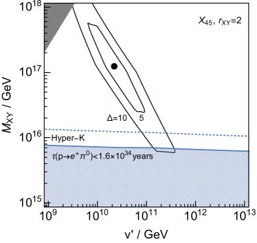
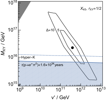
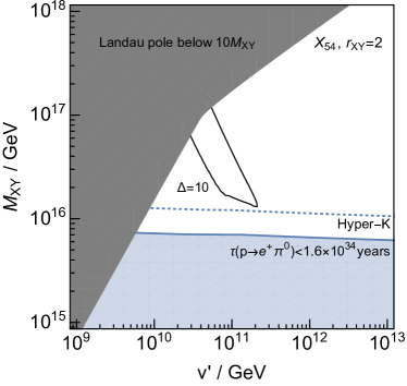
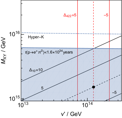
In Fig. 3, we show contours of in the plane, assuming (left) and (right). The dot indicates the point where . In the upper/lower panel, we assume that the multiplet generating the up yukawa couplings is . We fix the masses so that the quark yukawa couplings are reproduced for . In the gray-shaded region, the Landau pole of the gauge coupling is less than , so that the precision of gauge coupling unification is spoiled. The blue-shaded region predicts too rapid a proton decay rate and is excluded by Super Kamiokande Abe et al. (2017). The blue dotted line shows the sensitivity of Hyper Kamiokande Abe et al. (2018).
As is varied so the required value of changes. However, in the case that the entire multiplet is degenerate, an order of magnitude change in only changes by , as this is a two loop effect. The different 3221 irreducible representations, , within a single multiplet receive non-degeneracies of only few 10% or less from gauge radiative corrections below . However, for successful flavor physics we allow order unity tree-level splittings between these masses leading to contributions to of , where is a quadratic Casimir, normalized to 1/2 for a fundamental representation. Order unity splittings can give , depending on the size and number of the multiplets.
In Appendix B we compute contributions to from scalar multiplets that break . is typically smaller than 1 if is the only such multiplet, while and multiplets allow for of a few and 10, respectively.
Higher dimensional interactions between the symmetry breaking field and the gauge field in general split the gauge coupling constants at the unification scale. Assuming a suppression scale of the reduced Planck mass, splittings from a dimension five operator typically give for a unification scale of GeV. In theories with CP symmetry at the unification scale, which solve the strong CP problem, the dimension five operator is forbidden, and the splittings from a dimension six operator typically give . At lower values of the unification scale these values of are reduced.
IV.2
We match the SM gauge coupling constants to those of the 422 theory at the mass,
| (20) |
Since the values of and are known, the successful embedding of into the Pati-Salam gauge group fixes the scale . To take into account a possible threshold correction, we define
| (21) |
The RGE equation of the gauge coupling constants is
| (22) |
Here we only show the contribution from the gauge bosons, the SM fermions, and . The contribution from the states is shown in Appendix A.
We match the 422 gauge couplings at the mass, , of the XY gauge boson, which is the only heavy gauge boson. The threshold corrections at are
| (23) |
where denote possible threshold corrections from scalars and fermions. For each , we quantify the required value of the threshold correction by
| (24) |
In Fig. 4, we show the contours of and . The parameter point where no threshold correction is required is already excluded by Super Kamiokande. A threshold correction of is necessary to evade the bound from proton decay. We estimate the typical magnitude of the threshold corrections from the unified scalar multiplets that break belonging to or in Appendix B, and show that is typically . This is because of the smallness of the contribution of scalar particles to the renormalization of gauge couplings. Threshold correction can be large if the theory near the unification scale is non-minimal; if the unified scale arises from the supersymmetry breaking scale, the threshold correction can be easily as large as 10.
V Yukawa Couplings
The predictions from Higgs Parity coupling unification are affected by threshold corrections to . The SM yukawa couplings are generated from the mixing of with the states when parity is broken by . The leading correction to is expected to arise from the generation of the top quark yukawa coupling. In this section we discuss how the SM yukawa couplings arise from the unified theory via interactions of (7). We also show that there is a simple understanding of why the mass ratio deviates from the simplest expectation from grand unification, as well as why the neutrino masses and the mixings are not as hierarchical as those of quarks. We also comment on a possible impact on leptogenesis Fukugita and Yanagida (1986).
The states arise from or representations of , whose decomposition into 3221 is shown in Table 2. and give up-type yukawa couplings and neutrino masses, while gives down-type quark and charged lepton yukawa couplings. We do not consider larger representations as they lead to the gauge couplings blowing-up below the unification scale. For complex 3221 representations, and , we omit their complex conjugates, and from the table. Non-singlet multiplets are decomposed into SM multiplets by giving the charge as a subscript; thus , which is an doublet, contains SM multiplets .
Terms in the Lagrangian of the theory that lead to quark and lepton masses are
| (25) |
where and are both in , and denotes possible insertions of fields with symmetry breaking vevs. Note is not an invariant, and hence requires a non-trivial . In the following we analyze the yukawa couplings in the 3221 theory. The discussion for the 422 theory is almost the same, as the 422 symmetry does not impose relations between the parameters in the 3221 theory except for one case that we mention below. We study the generation of yukawa couplings in the up, down, charged lepton and neutrino sectors by integrating out the states.
| 54 | |||||
|---|---|---|---|---|---|
| 3 | 6 | 8 | 1 | 1 | |
| 2 | 1 | 1 | 3 | 1 | |
| 2 | 1 | 1 | 3 | 1 | |
| 0 | 0 | 0 | |||
| 45 | ||||||
|---|---|---|---|---|---|---|
| 3 | 3 | 8 | 1 | 1 | 1 | |
| 2 | 1 | 1 | 3 | 1 | 1 | |
| 2 | 1 | 1 | 1 | 3 | 1 | |
| 2/3 | 0 | 0 | 0 | 0 | ||
| 10 | ||
|---|---|---|
| 3 | 1 | |
| 1 | 2 | |
| 1 | 2 | |
V.1 Up-type quark yukawa couplings
The states for the up-type yukawas couplings are in or . For , the up yukawa couplings arise from the interaction and mass term
| (26) |
Note that below the breaking scale, the couplings and masses are given for each 3221 component of . We allow these couplings and masses to deviate from strict relations by order unity amounts via .
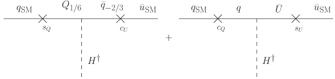
Here and below we neglect flavor mixing, which can be straightforwardly taken into account, so that and are real parameters referring to a single generation. We show how the SM up-type yukawa coupling arises in the upper most panel of Fig. 5. Because of the non-zero , and mix with each other. The mixings in Fig. 5 are given by
| (27) |
A linear combination of and obtains a mass , paired with . The orthogonal linear combination of and becomes a doublet quark of the SM acquiring a yukawa coupling to , a right-handed up-type quark, of
| (28) |
Except for the top yukawa coupling, we expect to be a good approximation, so that for the up and charm quarks. and obtain a mass .
When the states arise from , we have
| (29) |
The fate of and are the same as for . A linear combination of and pairs with and obtains a mass . The orthogonal combination becomes a of the SM, so that the corresponding up-type yukawa coupling is
| (30) |
Small up and charm yukawa couplings are explained by or .
V.2 Down-type quark yukawa coupling
The states for down-type quark yukawa couplings are in of , as larger representations result in non-perturbative gauge couplings. Yukawa couplings arise from
| (31) |
A linear combination of and obtains a mass , paired with . The orthogonal linear combination is the SM right-handed down quark. The SM down-type yukawa coupling is
| (32) |

V.3 Charged lepton yukawa couplings
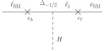
The states for charged lepton yukawa couplings are also in of , and the yukawa couplings arise from
| (33) |
A linear combination of and obtains a mass , paired with . The orthogonal linear combination is the SM lepton doublet.
The SM charged lepton yukawa couplings depend on whether the states for the up-type quark is or . If it is , is the SM right-handed charged lepton. If it is , we need to take into account the following interaction,
| (34) |
A linear combination of and obtains a mass , paired with . The orthogonal linear combination is the SM right-handed charged lepton. The SM charged lepton yukawa coupling is
| (35) |
V.4 Neutrino masses and mixing
If the states of up-type quarks are , neutrino masses may arise from the interactions and mass term,
| (36) |
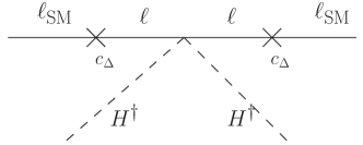
In the 422 theory and . At tree-level, only one linear combination of and , which is predominantly , obtains a mass, and the SM neutrino remains massless. However, since lepton and chiral symmetries are broken by , there is no symmetry forbidding a SM neutrino mass, which should arise from quantum corrections. Taking into account mixing between and , the neutrino mass is
| (37) |
If the states of up-type quarks are , the neutrino mass arises from Eq. (34),
| (38) |
Next we consider aspects of flavor mixing. Although the same states, , contribute to both up-type quark and neutrino masses, the lack of mass hierarchies and large mixing angles of neutrinos compared with up-type quarks can be understood. Assuming only for the third generation, the neutrino mass matrix is given by
| (39) |
where the factor of applies only for . With , the neutrino mass matrix is not near-diagonal nor hierarchical, except for the component. Thus, in Higgs Parity Unification we are able to derive an order-of-magnitude mass relation
| (40) |
which is successful since the Higgs mass and coupling unification require GeV. The small up quark mass arises from the component of (39), so that the lightest neutrino is much lighter than the other two neutrinos, goiving a normal hierarchy with
| (41) |
Because of the suppression of the neutrino mass by , for a given mass the couplings are larger than expected from the usual see-saw relation . We expect that the lepton asymmetry produced by decays of and is enhanced, reducing the minimal reheating temperature for successful leptogenesis, whether thermal Giudice et al. (2004); Buchmuller et al. (2005) or non-thermal Ibe et al. (2005).
V.5 A simple theory of flavor
The following renormalizable model can economically describe all quark and lepton masses
| (42) |
Here we introduce three generations of fermions, , and , with generation indices understood. The Higgs and are embedded into . is an symmetry breaking field, and , and are constants. Since does not appear in the above yukawa interactions, this model predicts and at the scale. However, while mass parameters are not necessarily unified, we assume that differing 3221 multiplets in the same representation have masses that are not hierarchically different from each other (e.g. ).
Despite the unification of , and departures from unification of by only amounts, the neutrino masses and mixings can be obtained via , as explained in the previous sub-section. This requires that both and are very close to unity, and hence and . Thus differs from that predicted in minimal unification schemes by , which arises from an O(1) difference between and . The ratios and can also be explained by ratios at the scale that are not far from unity.
The strong CP problem is solved by Left-Right symmetry including space-time parity. Above the breaking scale, the symmetry of the theory is . This symmetry is broken down to Left-Right symmetry with space-time parity by the VEV of a field that is both Left-Right and CP odd. The CP symmetry requires that and are real. When is made from an odd number of the Left-Right and CP odd fields, the couplings are pure-imaginary, explaining the CKM phase.
Ref. Hall and Harigaya (2018) shows that the quantum corrections to the strong CP phase arise at two-loop level. The corrections are shown to be below the current limit from the neutron electric dipole moment under the assumption that the couplings are and are above . This assumption is not valid for the components of and . As a result, the suppression of the corrections found in Hall and Harigaya (2018) is not guaranteed, and the corrections may be as large as . We expect that the corrections are suppressed by an appropriate flavor structure of and , which we leave to future work.
V.6 The bottom-tau mass ratio and
If the top quark mass is generated by , then the bottom quark but not the tau, receives a suppression from the up-type quark yukawa sector; thus from Eqs. (32) and (35) while . Assuming at the unification scale, as well as to obtain the neutrino masses and mixing, we find at the unified scale, which is renormalized to
| (43) |
To obtain the observed ratio of , we need
| (44) |
If the top quark mass is generated by , the tau yukawa coupling may be also suppressed by . To obtain the bottom/tau ratio, is required. Unless , we may neglect the suppression of the tau yukawa coupling. Assuming at the unification scale as well as , the observed value of then requires
| (45) |
where we assume and .
VI Prediction for the Scale of Parity Breaking
In Sec. II, we showed that the SM Higgs quartic coupling essentially vanishes at tree level at the Higgs Parity symmetry breaking scale, . In this section, we compute threshold corrections to the Higgs quartic coupling and derive in terms of SM parameters.
VI.1 Threshold corrections to the SM quartic coupling
The tree-level scalar potential is
| (46) |
After taking into account quantum corrections, the coupling becomes non-zero.
VI.1.1 Threshold correction from charged gauge bosons
The one-loop Coleman-Weinberg (CW) potential from and bosons is
| (47) |
where is an arbitrary scale. A change of can be absorbed by a change of . The vev of satisfies
| (48) |
After integrating out , the potential for , to leading order in and , is given by
| (49) |
To obtain the electroweak scale much smaller than requires , giving
| (50) |
We match this potential to the one-loop CW potential of the SM from the boson,
where we take the scheme. By matching to with , we obtain
| (51) |
To suppress higher order corrections, the coupling should be evaluated around .
VI.1.2 Threshold correction from neutral gauge bosons
The threshold correction from and bosons can be estimated in a similar manner. After integrating out and fine-tuning for the electroweak scale, the Higgs potential is
| (52) |
The one-loop CW potential of the SM from the boson is
| (53) |
Matching these results at gives the threshold correction
| (54) |
VI.1.3 Threshold correction from top quarks
The threshold correction from top quarks is model-dependent. Let us first consider the case where the state for the top quark is , where the relevant interaction is shown in Eq. (26). The mass squareds of the six mass eigenstates are
| (55) |
With a similar computation to the gauge contribution, we find that
| (56) | |||
| (57) |
The one-loop CW potential of the SM from the top quark is
| (58) |
and matching these potentials yields the threshold correction
| (59) |
Note that the threshold correction logarithmically diverges as i.e. because, for , there is an additional particle below the scale coupling to the SM Higgs.
We next consider the case where the state for the top quark is , where the relevant interactions are shown in Eq. (29). We only consider the case and , giving the top yukawa coupling
| (60) |
which can be solved for
| (61) |
We find the threshold correction
| (62) |
where the functions are given by
| (63) |
The function nearly vanishes around .
VI.1.4 Threshold correction from other fermions
The threshold correction from other charged fermions are expected to be negligibly small because the corresponding or . An exceptional case arises if the up/charm yukawas, arise from , and follows from while . We do not consider such a case.
The threshold correction from the neutrino that is in the same as the top quark can be large since and . If the state for the top quark is , the yukawa coupling of and to and are of the form (36), which is symmetric. The threshold correction to vanishes at one-loop level. If the state for the top quark is , the yukawa coupling is of the form
| (64) |
giving the threshold correction
| (65) |
We find this correction to be negligible unless , which requires and is disfavored from the bottom-tau ratio.
VI.1.5 Threshold correction from colored Higgses in the 422 theory
In the 422 theory, colored Higgs have masses around the scale , and contribute to the threshold correction to . We denote the and Higgses as and , respectively. Here , , are the , , indices, respectively. The invariant potential is given in general by
| (66) |
where . The threshold correction is given by Hall and Harigaya (2018)
| (67) | ||||
| (68) |
The function is always negative and is typically . As long as , , are less than , this contribution is subdominant. If , , are larger than unity, which leads to strongly coupled Higgses at higher energy scales, this contribution can be large and predicts larger top quark masses. We assume weakly coupled Higgs bosons and neglect the threshold correction from the colored Higgses.
VI.2 Top quark mass, QCD coupling and the Higgs Parity breaking scale
Let us first clarify the top quark mass we use in this paper. We use the pole top quark mass , from which we compute the top yukawa coupling via Buttazzo et al. (2013)
| (69) |
where the NNNLO QCD quantum correction is included. The conversion necessarily involves an uncertainty due to the non-perturbative nature of QCD Bigi et al. (1994); Beneke and Braun (1994); Beneke (1999). To go beyond the precision limited by this uncertainty, which is expected to be as large as the QCD scale, the top quark mass shown in this paper should be understood as a quantity defined by Eq. (69). Also, the pole mass measured using hadronic final states suffers from the uncertainty of soft QCD processes including hadronization Skands and Wicke (2007). We nevertheless show the value suggested in Tanabashi et al. (2018), GeV, as a guide.
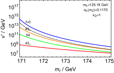
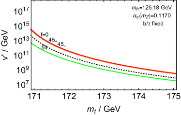
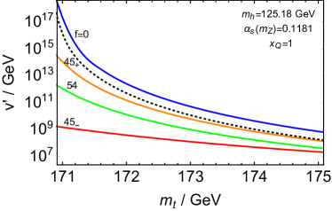
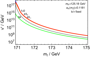
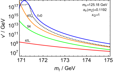
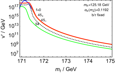
We compute the running of the SM Higgs quartic coupling following Buttazzo et al. (2013). In Fig. 6 we show the prediction for the Higgs Parity breaking scale as a function of the top quark mass for various values of the QCD coupling constant and choices of the states. In the left panels, we take . For a given top quark mass, the prediction for is smaller than the one for , since . We find that this is also the case for with generic . Thus, for a given , which is fixed by successful unification, we obtain an upper bound on the top quark mass.
We can make a sharper prediction by assuming bottom-tau unification discussed in Sec. V.6. In the right panels, we take the value of to reproduce the bottom/tau ratio. The predictions for are indistinguishable from the one for . Here it is assumed that . We find that this is still the case for , while for the result approaches that of . The prediction for differs from , but not by as much as when . For this case of the simplest successful result, for a given we have two predictions for the top quark mass, which differ from each other by GeV.
VII Precise Unification and SM parameters
In Sec. IV we used gauge coupling unification to predict the unified mass scale and the Higgs Parity breaking scale in terms of unified threshold corrections from gauge particles, , and from scalars and fermions, , as shown in Figs. 3 and 4. In Sec. VI, was predicted by evolution of the SM quartic, including threshold corrections from this Higgs Parity breaking scale that are sensitive to the top quark coupling , as shown in Fig. 6. By combining these results from Secs. IV and VI, which both depend on whether the state for the top quark mass is a or , we are finally ready to discuss the correlation among SM parameters discussed in the introduction.
VII.1
In Fig. 7, the predicted correlation between and is shown, for chosen to fix . In the left panel, regions with or 3 are shaded, which is reasonable if the Higgses are or . For a given theory, is predicted with uncertainties of
| (70) |
The range of and Tanabashi et al. (2018) is shown by a dotted box.
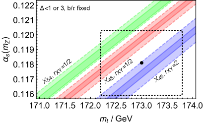
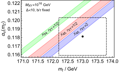
Note that, with fixed by , a top mass from gives . Since for and for any breaking to 3221 via Higgs of , the prediction labelled as can be understood as a model-independent upper bound on the top quark mass. For example, if , assuming , the top quark mass must be below GeV. The sensitivity of the prediction on to the value of is shown in Fig. 8 for and . The prediction on decreases by GeV if is larger than the one to fix by more than few 10%.

The running of the gauge and quartic couplings for the experimental central value of is shown in Fig. 1, assuming , and fixing . The global picture of the correlation shown in Fig. 2 also assumes the same setup, although the picture looks similar for other choices of the states, and .
In the right panel of Fig. 7, we fix the gauge boson mass to be GeV, which would be suggested if proton decay is observed by Hyper-K. A large value for is then needed for unification, and the widths of the shaded bands result from requiring . The top quark mass must be below GeV for . If proton decay is observed by Hyper-K and the top quark mass is found to be near this bound, we can infer that the bottom-tau ratio is fixed by and symmetry is broken by a VEV.
VII.2
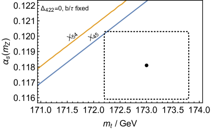
In the 422 theory, the embedding of the coupling into the couplings is non-trivial. In the minimal theory, the threshold correction only arises from the colored Higgs,
| (71) |
where is the mass of the colored Higgs whose gauge quantum number is the same as that of the SM quark doublet. The magnitude of this correction is less than , unless the parameters of the Higgs potential are fine-tuned to make the colored Higgs much lighter than . A contribution to may also arise from the mass splitting of states. As long as and preserve approximate grand unified relations, this contribution is also small. One may wonder whether the hierarchy of leads to a large threshold correction. This is not the case since the VEV of breaks only to .
For , GeV is required. In Fig. 9, the predicted correlation between and is shown, for chosen to fix . Note that, for this choice of , a top mass from gives . Since , the prediction labelled as can be understood as a model-independent upper bound on the top quark mass. The top quark mass/QCD coupling constant is predicted to be significantly smaller/larger than the central value.
VIII Discussion
Higgs Parity accounts for a remarkable coincidence: the scale at which the SM quartic coupling vanishes is close to the scale of Left-Right symmetry breaking required for gauge coupling unification in , as illustrated in Fig. 1. In this paper we have explored in detail the precision of this coincidence, which we frame in terms of a correlation of the measured values of the top quark mass and the QCD coupling.
Taking the intermediate gauge symmetry to be 3221, the global picture of this correlation is shown in the right panel of Fig. 2, and the fine detail close to the experimental values is shown in the left panel of Fig. 7. This correlation is indeed remarkable, and appears at least as precise as the correlation of the QCD coupling with the weak mixing angle in supersymmetric unification. The constraint on the 3221 breaking scale from gauge coupling unification alone is shown in Fig. 3, and is roughly GeV. This should be compared with the constraint on from running the SM quartic coupling, shown in Fig. 6, which is significantly affected by the threshold effect from a coupling of the top quark sector. If this parameter is the dominant effect reconciling with unified yukawa couplings, then this constraint on is sharpened. Matching the values of from gauge coupling unification and SM quartic running, and allowing typical threshold corrections in simple models of breaking, then yields a successful prediction at high precision: to 1%, or to 0.2%, as illustrated in the left panel of Fig. 7.
The precision may be reduced in more complicated models, or if large breaking effects enter the spectrum or couplings of the states that generate yukawa couplings. However, as experimental uncertainties on and are reduced, evidence may accumulate for a particular simple version of Higgs Parity unification. For example, future measurements leading to the blue region of the left panel of Fig. 7 would provide evidence for a simple model with: broken via a 45 to 3221, small unified corrections from scalars and fermions, exchange generating the top yukawa coupling, and resulting from mixing of states between this and the third generation matter .
The dominant sensitivity to in this correlation arises from the determination of from the running of the quartic, not from the determination of from gauge coupling unification. This implies that the sensitivity of the prediction for to the grand unified thresholds, , as shown by the widths of the shadings in the left panel of Fig. 7, is about an order of magnitude less in Higgs Parity unification than in conventional grand unification.
Taking the intermediate gauge symmetry to be 422 leads to a much larger value for from gauge coupling unification: GeV, even allowing quite large unified threshold corrections, as shown in Fig. 4. To match the value of from running of the SM quartic coupling then favors values that successfully determine , but only for large values of and small values of , as shown in Fig. 9.
In the 3221 theory with minimal content for the breaking Higgs, the unification scale is above GeV and the proton lifetime is predicted to be above the current constraint, as shown in the left panels of Fig. 3. An observation of proton decay at future experiments would require large threshold corrections at the unification scale, , and/or non-minimal breaking. In both cases, a larger and hence a smaller top quark mass is favored, as illustrated in the right panel of Fig. 7.
In the 422 theory, threshold corrections at the unification scale from breaking Higgses give . As Fig. 4 shows, the theory predicts the unification scale around GeV and hence too short a proton lifetime. The unification scale can be raised to GeV by large threshold corrections, , which requires a rich structure around the unification scale such as symmetry breaking induced by supersymmetry breaking.
The observed flavor structure of the SM may arise from an unified theory, as suggested in Eq. (V.5). Although we have not performed precise fits to the SM fermion masses, it would be interesting to do so and to investigate relations between the flavor observables. The model appears to predict a neutrino mass matrix proportional to the up quark mass matrix. However, this is avoided because of mixing between the third generation and fermions at the scale . The theory of Eq. (V.5) predicts , while the prediction is smaller by a factor of if is replaced by ; both cases give a normal neutrino mass hierarchy. To obtain realistic neutrino masses requires GeV, which coincides with the scale required from gauge coupling unification and the vanishing SM quartic coupling. Because of the suppression, the yukawa coupling of the right-handed neutrinos responsible for the see-saw mechanism is larger than naively expected from the see-saw relation, increasing the efficiency of leptogenesis and allowing lower reheat temperatures than usual.
In conventional theories, the amount of fine tuning for symmetry breaking increases as the intermediate scale is reduced below the unification scale. However, with Higgs Parity the amount of fine tuning is independent of the intermediate scale, and corresponds to the usual cost of keeping the weak scale below the cutoff.
Acknowledgement
This work was supported in part by the Director, Office of Science, Office of High Energy and Nuclear Physics, of the US Department of Energy under Contracts DE-AC02-05CH11231 (LH) and DE-SC0009988 (KH), as well as by the National Science Foundation under grants PHY-1316783 and PHY-1521446 (LH).
Appendix A Contributions of States to Beta Functions
In this Appendix we give the contributions of the states to the beta functions of the gauge couplings at two-loop level. We define the coefficient of the beta function by
| (72) |
The contributions of each multiplet to the coefficients of the 3221 theory are
| (73) | ||||
| (74) | ||||
| (75) |
and for the coefficients of the 422 theory are
| (76) | ||||
| (77) | ||||
| (78) |
Appendix B Threshold Corrections from Breaking Scalars
In this Appendix we derive the threshold corrections to the gauge coupling unification from scalar multiplets that spontaneously break .
B.1
The smallest representation which can break down to is . This case is particularly interesting as the strong CP problem is solved by assigning an odd CP parity to . The decomposition of into non-trivial representations, and the contribution of each of these to the beta functions, is summarized in Table 3. The representations and are would-be Nambu-Goldstone bosons. The threshold corrections to the gauge couplings are
| (79) | ||||
| (80) | ||||
| (81) |
The contributions of to are
| (82) |
As shown in Yasue (1981a, b); Anastaze et al. (1983); Bertolini et al. (2010), after choosing the parameters of the potential to avoid tachyonic directions, . Their masses are given by quantum corrections, taking natural values of about . Even with this hierarchy, are only .
| 45 | |||||
| 3 | 3 | 8 | 1 | 1 | |
| 2 | 1 | 1 | 3 | 1 | |
| 2 | 1 | 1 | 1 | 3 | |
| 2/3 | 0 | 0 | 0 | ||
| 2/3 | 1/6 | 1/2 | 0 | ||
| 1 | 0 | 0 | 1/3 | ||
| 2/3 | 2/3 | 0 | 0 | ||
| 54 | ||||
| 3 | 6 | 8 | 1 | |
| 2 | 1 | 1 | 3 | |
| 2 | 1 | 1 | 3 | |
| 0 | 0 | |||
| 2/3 | 5/6 | 1/2 | 0 | |
| 1 | 0 | 0 | 1 | |
| 2/3 | 4/3 | 0 | 0 | |
| 210 | ||||||||||||
| 3 | 3 | 8 | 1 | 1 | 3 | 3 | 8 | 8 | 6 | 3 | 1 | |
| 2 | 1 | 1 | 3 | 1 | 3 | 1 | 3 | 1 | 2 | 2 | 2 | |
| 2 | 1 | 1 | 1 | 3 | 1 | 3 | 1 | 3 | 2 | 2 | 2 | |
| 2/3 | 0 | 0 | 0 | 2/3 | 2/3 | 0 | 0 | 1/3 | -1 | |||
| 2/3 | 1/6 | 1/2 | 0 | 1 | 3 | 10/3 | 2/3 | 0 | ||||
| 1 | 0 | 0 | 1/3 | 2 | 8/3 | 2 | 1 | 1/3 | ||||
| 2/3 | 2/3 | 0 | 0 | 4 | 0 | 4/3 | 2/3 | 2 | ||||
We also consider whose decomposition is shown in Table 3. Although can break down only to , its presence allows all components of to have positive mass squared at tree-level Babu and Ma (1985). The threshold corrections from and are
| (83) |
With mass splittings, these threshold corrections can be . With mass splittings of , can be ; however such scalar mass hierarchies require fine-tuning of parameters.
We conclude that, in a theory with the strong CP problem solved by Higgs Parity, unified threshold corrections to gauge couplings are typically . However, threshold corrections can be large if the theory is non-minimal or the mass spectrum is fine-tuned, or if significant breaking feeds into the spectrum of states.
The next smallest representation is , whose decomposition is shown in Table 3. This representation is required if CP is not imposed on the theory. The contribution of to is
| (84) |
Depending on the mass spectrum, may be as large as 10 even if the mass splittings are of .
B.2
| 54 | |||
| 6 | 1 | ||
| 2 | 1 | 3 | |
| 2 | 1 | 3 | |
| 2/3 | 4/3 | 0 | |
| 1 | 0 | 1 | |
| 210 | |||||
| 6 | 15 | 15 | 15 | 10 | |
| 2 | 1 | 3 | 1 | 2 | |
| 2 | 1 | 1 | 3 | 2 | |
| 2/3 | 2/3 | 4 | 4 | ||
| 1 | 0 | 5 | 10/3 | ||
The smallest representation which can break down to is . The decomposition of into the representations and the contribution of each to the beta functions are summarized in Table 4. The threshold corrections to the gauge couplings are
| (85) |
Hence, the contribution of to is
| (86) |
which is a few at most, even if the mass splitting is .
The next smallest representation for breaking to 422 is , whose decomposition is shown in Table 4. The strong CP problem is solved by assigning an odd CP parity to . The contribution of to is
| (87) |
which is at most a few, even if the mass splitting is .
References
- Aad et al. (2012) G. Aad et al. (ATLAS), Phys. Lett. B716, 1 (2012), arXiv:1207.7214 [hep-ex] .
- Chatrchyan et al. (2012) S. Chatrchyan et al. (CMS), Phys. Lett. B716, 30 (2012), arXiv:1207.7235 [hep-ex] .
- Aaboud et al. (2018) M. Aaboud et al. (ATLAS), Phys. Rev. D97, 112001 (2018), arXiv:1712.02332 [hep-ex] .
- Sirunyan et al. (2018) A. M. Sirunyan et al. (CMS), JHEP 05, 025 (2018), arXiv:1802.02110 [hep-ex] .
- Georgi et al. (1974) H. Georgi, H. R. Quinn, and S. Weinberg, Phys. Rev. Lett. 33, 451 (1974).
- Georgi and Glashow (1974) H. Georgi and S. L. Glashow, Phys. Rev. Lett. 32, 438 (1974).
- Chanowitz et al. (1977) M. S. Chanowitz, J. R. Ellis, and M. K. Gaillard, Nucl. Phys. B128, 506 (1977).
- Decamp et al. (1990) D. Decamp et al. (ALEPH), Z. Phys. C48, 365 (1990).
- Dimopoulos et al. (1981) S. Dimopoulos, S. Raby, and F. Wilczek, Phys. Rev. D24, 1681 (1981).
- Dimopoulos and Georgi (1981) S. Dimopoulos and H. Georgi, Nucl. Phys. B193, 150 (1981).
- Sakai (1981) N. Sakai, Z. Phys. C11, 153 (1981).
- Ibanez and Ross (1981) L. E. Ibanez and G. G. Ross, Phys. Lett. 105B, 439 (1981).
- Einhorn and Jones (1982) M. B. Einhorn and D. R. T. Jones, Nucl. Phys. B196, 475 (1982).
- Marciano and Senjanovic (1982) W. J. Marciano and G. Senjanovic, Phys. Rev. D25, 3092 (1982).
- Buttazzo et al. (2013) D. Buttazzo, G. Degrassi, P. P. Giardino, G. F. Giudice, F. Sala, A. Salvio, and A. Strumia, JHEP 12, 089 (2013), arXiv:1307.3536 [hep-ph] .
- Hall and Nomura (2014) L. J. Hall and Y. Nomura, JHEP 02, 129 (2014), arXiv:1312.6695 [hep-ph] .
- Hall et al. (2014a) L. J. Hall, Y. Nomura, and S. Shirai, JHEP 06, 137 (2014a), arXiv:1403.8138 [hep-ph] .
- Hall and Harigaya (2018) L. J. Hall and K. Harigaya, JHEP 10, 130 (2018), arXiv:1803.08119 [hep-ph] .
- Dunsky et al. (2019) D. Dunsky, L. J. Hall, and K. Harigaya, (2019), arXiv:1902.07726 [hep-ph] .
- Georgi (1975) H. Georgi, PARTICLES AND FIELDS — 1974: Proceedings of the Williamsburg Meeting of APS/DPF, AIP Conf. Proc. 23, 575 (1975).
- Fritzsch and Minkowski (1975) H. Fritzsch and P. Minkowski, Annals Phys. 93, 193 (1975).
- Pati and Salam (1974) J. C. Pati and A. Salam, Phys. Rev. D10, 275 (1974), [Erratum: Phys. Rev.D11,703(1975)].
- Beg and Tsao (1978) M. A. B. Beg and H. S. Tsao, Phys. Rev. Lett. 41, 278 (1978).
- Mohapatra and Senjanovic (1978) R. N. Mohapatra and G. Senjanovic, Phys. Lett. 79B, 283 (1978).
- Kibble et al. (1982) T. W. B. Kibble, G. Lazarides, and Q. Shafi, Phys. Lett. 113B, 237 (1982).
- Chang et al. (1984a) D. Chang, R. N. Mohapatra, and M. K. Parida, Phys. Rev. Lett. 52, 1072 (1984a).
- Chang et al. (1984b) D. Chang, R. N. Mohapatra, and M. K. Parida, Phys. Rev. D30, 1052 (1984b).
- Lazarides and Shafi (1985) G. Lazarides and Q. Shafi, Phys. Lett. 159B, 261 (1985).
- Barr et al. (1991) S. M. Barr, D. Chang, and G. Senjanovic, Phys. Rev. Lett. 67, 2765 (1991).
- Kuchimanchi (1996) R. Kuchimanchi, Phys. Rev. Lett. 76, 3486 (1996), arXiv:hep-ph/9511376 [hep-ph] .
- Mohapatra and Rasin (1996a) R. N. Mohapatra and A. Rasin, Phys. Rev. Lett. 76, 3490 (1996a), arXiv:hep-ph/9511391 [hep-ph] .
- Mohapatra and Rasin (1996b) R. N. Mohapatra and A. Rasin, Phys. Rev. D54, 5835 (1996b), arXiv:hep-ph/9604445 [hep-ph] .
- Mohapatra et al. (1997) R. N. Mohapatra, A. Rasin, and G. Senjanovic, Phys. Rev. Lett. 79, 4744 (1997), arXiv:hep-ph/9707281 [hep-ph] .
- Kuchimanchi (2010) R. Kuchimanchi, Phys. Rev. D82, 116008 (2010), arXiv:1009.5961 [hep-ph] .
- D’Agnolo and Hook (2016) R. T. D’Agnolo and A. Hook, Phys. Lett. B762, 421 (2016), arXiv:1507.00336 [hep-ph] .
- Albaid et al. (2015) A. Albaid, M. Dine, and P. Draper, JHEP 12, 046 (2015), arXiv:1510.03392 [hep-ph] .
- Babu et al. (2019) K. S. Babu, B. Dutta, and R. N. Mohapatra, JHEP 01, 168 (2019), arXiv:1811.04496 [hep-ph] .
- Mimura et al. (2019) Y. Mimura, R. N. Mohapatra, and M. Severson, (2019), arXiv:1903.07506 [hep-ph] .
- Babu and Mohapatra (1989) K. S. Babu and R. N. Mohapatra, Phys. Rev. Lett. 62, 1079 (1989).
- Babu and Mohapatra (1990) K. S. Babu and R. N. Mohapatra, Phys. Rev. D41, 1286 (1990).
- Agrawal et al. (1998) V. Agrawal, S. M. Barr, J. F. Donoghue, and D. Seckel, Phys. Rev. D57, 5480 (1998), arXiv:hep-ph/9707380 [hep-ph] .
- Hall et al. (2014b) L. J. Hall, D. Pinner, and J. T. Ruderman, JHEP 12, 134 (2014b), arXiv:1409.0551 [hep-ph] .
- Abe et al. (2017) K. Abe et al. (Super-Kamiokande), Phys. Rev. D95, 012004 (2017), arXiv:1610.03597 [hep-ex] .
- Abe et al. (2018) K. Abe et al. (Hyper-Kamiokande), (2018), arXiv:1805.04163 [physics.ins-det] .
- Fukugita and Yanagida (1986) M. Fukugita and T. Yanagida, Phys. Lett. B174, 45 (1986).
- Giudice et al. (2004) G. F. Giudice, A. Notari, M. Raidal, A. Riotto, and A. Strumia, Nucl. Phys. B685, 89 (2004), arXiv:hep-ph/0310123 [hep-ph] .
- Buchmuller et al. (2005) W. Buchmuller, P. Di Bari, and M. Plumacher, Annals Phys. 315, 305 (2005), arXiv:hep-ph/0401240 [hep-ph] .
- Ibe et al. (2005) M. Ibe, T. Moroi, and T. Yanagida, Phys. Lett. B620, 9 (2005), arXiv:hep-ph/0502074 [hep-ph] .
- Bigi et al. (1994) I. I. Y. Bigi, M. A. Shifman, N. G. Uraltsev, and A. I. Vainshtein, Phys. Rev. D50, 2234 (1994), arXiv:hep-ph/9402360 [hep-ph] .
- Beneke and Braun (1994) M. Beneke and V. M. Braun, Nucl. Phys. B426, 301 (1994), arXiv:hep-ph/9402364 [hep-ph] .
- Beneke (1999) M. Beneke, Phys. Rept. 317, 1 (1999), arXiv:hep-ph/9807443 [hep-ph] .
- Skands and Wicke (2007) P. Z. Skands and D. Wicke, Eur. Phys. J. C52, 133 (2007), arXiv:hep-ph/0703081 [HEP-PH] .
- Tanabashi et al. (2018) M. Tanabashi et al. (Particle Data Group), Phys. Rev. D98, 030001 (2018).
- Yasue (1981a) M. Yasue, Phys. Rev. D24, 1005 (1981a).
- Yasue (1981b) M. Yasue, Phys. Lett. 103B, 33 (1981b).
- Anastaze et al. (1983) G. Anastaze, J. P. Derendinger, and F. Buccella, Z. Phys. C20, 269 (1983).
- Bertolini et al. (2010) S. Bertolini, L. Di Luzio, and M. Malinsky, Phys. Rev. D81, 035015 (2010), arXiv:0912.1796 [hep-ph] .
- Babu and Ma (1985) K. S. Babu and E. Ma, Phys. Rev. D31, 2316 (1985).