An adaptive nearest neighbor rule for classification

Akshay Balsubramani
abalsubr@stanford.edu
&Sanjoy Dasgupta
dasgupta@eng.ucsd.edu
&Yoav Freund
yfreund@eng.ucsd.edu
&Shay Moran
shaym@princeton.edu
Abstract

We introduce a variant of the kπ‘˜k-nearest neighbor classifier in which kπ‘˜k is chosen adaptively for each query, rather than supplied as a parameter. The choice of kπ‘˜k depends on properties of each neighborhood, and therefore may significantly vary between different points. (For example, the algorithm will use larger kπ‘˜k for predicting the labels of points in noisy regions.)

We provide theory and experiments that demonstrate that the algorithm performs comparably to, and sometimes better than, kπ‘˜k-NN with an optimal choice of kπ‘˜k. In particular, we derive bounds on the convergence rates of our classifier that depend on a local quantity we call the β€œadvantage” which is significantly weaker than the Lipschitz conditions used in previous convergence rate proofs. These generalization bounds hinge on a variant of the seminal Uniform Convergence Theorem due to Vapnik and Chervonenkis; this variant concerns conditional probabilities and may be of independent interest.

1 Introduction

We introduce an adaptive nearest neighbor classification rule. Given a training set with labels {Β±1}plus-or-minus1\{\pm 1\}, its prediction at a query point xπ‘₯x is based on the training points closest to xπ‘₯x, rather like the kπ‘˜k-nearest neighbor rule. However, the value of kπ‘˜k that it uses can vary from query to query. Specifically, if there are n𝑛n training points, then for any query xπ‘₯x, the smallest kπ‘˜k is sought for which the kπ‘˜k points closest to xπ‘₯x have labels whose average is either greater than +Δ​(n,k)Ξ”π‘›π‘˜+\Delta(n,k), in which case the prediction is +11+1, or less than βˆ’Ξ”β€‹(n,k)Ξ”π‘›π‘˜-\Delta(n,k), in which case the prediction is βˆ’11-1; and if no such kπ‘˜k exists, then β€œ?” (β€œdon’t know”) is returned. Here, Δ​(n,k)∼(log⁑n)/ksimilar-toΞ”π‘›π‘˜π‘›π‘˜\Delta(n,k)\sim\sqrt{(\log n)/k} corresponds to a confidence interval for the average label in the region around the query.

We study this rule in the standard statistical framework in which all data are i.i.d.Β draws from some unknown underlying distribution P𝑃P on 𝒳×𝒴𝒳𝒴{\mathcal{X}}\times{\mathcal{Y}}, where 𝒳𝒳{\mathcal{X}} is the data space and 𝒴𝒴{\mathcal{Y}} is the label space. We take 𝒳𝒳{\mathcal{X}} to be a separable metric space, with distance function d:𝒳×𝒳→ℝ:𝑑→𝒳𝒳ℝd:{\mathcal{X}}\times{\mathcal{X}}\rightarrow{\mathbb{R}}, and we take 𝒴={Β±1}𝒴plus-or-minus1{\mathcal{Y}}=\{\pm 1\}. We can decompose P𝑃P into the marginal distribution ΞΌπœ‡\mu on 𝒳𝒳{\mathcal{X}} and the conditional expectation of the label at each point xπ‘₯x: if (X,Y)π‘‹π‘Œ(X,Y) represents a random draw from P𝑃P, define η​(x)=𝔼​(Y|X=x)πœ‚π‘₯𝔼conditionalπ‘Œπ‘‹π‘₯\eta(x)={\mathbb{E}}(Y|X=x). In this terminology, the Bayes-optimal classifier is the rule gβˆ—:𝒳→{Β±1}:superscript𝑔→𝒳plus-or-minus1g^{*}:{\mathcal{X}}\rightarrow\{\pm 1\} given by

gβˆ—β€‹(x)={sign​(η​(x))if η​(x)β‰ 0eitherΒ βˆ’1Β orΒ +1if η​(x)=0superscript𝑔π‘₯casessignπœ‚π‘₯ifΒ Ξ·(x)β‰ 0eitherΒ βˆ’1Β orΒ +1ifΒ Ξ·(x)=0g^{*}(x)=\left\{\begin{array}[]{ll}\mbox{sign}(\eta(x))&\mbox{if $\eta(x)\neq 0$}\\ \mbox{either $-1$ or $+1$}&\mbox{if $\eta(x)=0$}\end{array}\right. (1)

and its error rate is the Bayes risk, Rβˆ—=12​𝔼XβˆΌΞΌβ€‹[1βˆ’|η​(X)|]superscript𝑅12subscript𝔼similar-toπ‘‹πœ‡delimited-[]1πœ‚π‘‹R^{*}=\frac{1}{2}{\mathbb{E}}_{X\sim\mu}\left[1-|\eta(X)|\right]. A variety of nonparametric classification schemes are known to have error rates that converge asymptotically to Rβˆ—superscript𝑅R^{*}. These include kπ‘˜k-nearest neighbor (henceforth, kπ‘˜k-NN) rulesΒ [FH51] in which kπ‘˜k grows with the number of training points n𝑛n according to a suitable schedule (kn)subscriptπ‘˜π‘›(k_{n}), under certain technical conditions on the metric measure space (𝒳,d,ΞΌ)π’³π‘‘πœ‡({\mathcal{X}},d,\mu).

In this paper, we are interested in consistency as well as rates of convergence. In particular, we find that the adaptive nearest neighbor rule is also asymptotically consistent (under the same technical conditions) while converging at a rate that is about as good as, and sometimes significantly better than, that of kπ‘˜k-NN under any schedule (kn)subscriptπ‘˜π‘›(k_{n}).

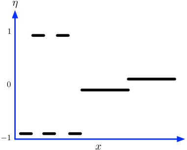
Intuitively, one of the advantages of kπ‘˜k-NN over nonparametric classifiers that use a fixed bandwidth or radius, such as Parzen window or kernel density estimators, is that kπ‘˜k-NN automatically adapts to variation in the marginal distribution ΞΌπœ‡\mu: in regions with large ΞΌπœ‡\mu, the kπ‘˜k nearest neighbors lie close to the query point, while in regions with small ΞΌπœ‡\mu, the kπ‘˜k nearest neighbors can be further afield. The adaptive NN rule that we propose goes further: it also adapts to variation in Ξ·πœ‚\eta. In certain regions of the input space, where Ξ·πœ‚\eta is close to 00, an accurate prediction would need large kπ‘˜k. In other regions, where Ξ·πœ‚\eta is near βˆ’11-1 or 111, a small kπ‘˜k would suffice, and in fact, a larger kπ‘˜k might be detrimental because neighboring regions might be labeled differently. See FigureΒ 1 for one such example. A kπ‘˜k-NN classifier is forced to pick a single value of kπ‘˜k that trades off between these two contingencies. Our adaptive NN rule, however, can pick the right kπ‘˜k in each neighborhood separately.

Refer to caption
Figure 1: For values of xπ‘₯x on the left half of the shown interval, the pointwise bias η​(x)πœ‚π‘₯\eta(x) is close to βˆ’11-1 or 111, and thus a small value of kπ‘˜k will yield an accurate prediction. Larger kπ‘˜k will not do as well, because they may run into neighboring regions with different labels. For values of xπ‘₯x on the right half of the interval, η​(x)πœ‚π‘₯\eta(x) is close to 00, and thus large kπ‘˜k is essential for accurate prediction.

Our estimator allows us to give rates of convergence that are tighter and more transparent than those customarily obtained in nonparametric statistics. Specifically, for any point xπ‘₯x in the instance space 𝒳𝒳{\mathcal{X}}, we define a notion of the advantage at xπ‘₯x, denoted adv​(x)advπ‘₯{\rm adv}(x), which is rather like a local margin. We show that the prediction at xπ‘₯x is very likely to be correct once the number of training points exceedsΒ O~​(1/adv​(x))~𝑂1advπ‘₯\tilde{O}(1/{\rm adv}(x)). Universal consistency follows by establishing that almost all points have positive advantage.

1.1 Relation to other work in nonparametric estimation

For linear separators and many other parametric families of classifiers, it is possible to give rates of convergence that hold without any assumptions on the input distribution ΞΌπœ‡\mu or the conditional expectation function Ξ·πœ‚\eta. This is not true of nonparametric estimation: although any target function can in principle be captured, the number of samples needed to achieve a specific level of accuracy will inevitably depend upon aspects of this function such as how fast it changesΒ [DGL96, chapter 7]. As a result, nonparametric statistical theory has focused on (1) asymptotic consistency, ideally without assumptions, and (2) rates of convergence under a variety of smoothness assumptions.

Asymptotic consistency has been studied in great detail for the kπ‘˜k-NN classifier, when kπ‘˜k is allowed to grow with the number of data points n𝑛n. The risk of the classifier, denoted Rnsubscript𝑅𝑛R_{n}, is its error rate on the underlying distribution P𝑃P; this is a random variable that depends upon the set of training points seen. Cover and HartΒ [CH67] showed that in general metric spaces, under the assumption that every xπ‘₯x in the support of ΞΌπœ‡\mu is either a continuity point of Ξ·πœ‚\eta or has μ​({x})>0πœ‡π‘₯0\mu(\{x\})>0, the expected risk 𝔼​Rn𝔼subscript𝑅𝑛{\mathbb{E}}R_{n} converges to the Bayes-optimal risk Rβˆ—superscript𝑅R^{*}, as long as kβ†’βˆžβ†’π‘˜k\rightarrow\infty and k/nβ†’0β†’π‘˜π‘›0k/n\rightarrow 0. For points in finite-dimensional Euclidean space, a series of results starting with StoneΒ [Sto77] established consistency without any assumptions on ΞΌπœ‡\mu or Ξ·πœ‚\eta, and showed that Rnβ†’Rβˆ—β†’subscript𝑅𝑛superscript𝑅R_{n}\rightarrow R^{*} almost surelyΒ [DGKL94]. More recent work has extended these universal consistency resultsβ€”that is, consistency without assumptions on Ξ·πœ‚\etaβ€”to arbitrary metric measure spaces (𝒳,d,ΞΌ)π’³π‘‘πœ‡({\mathcal{X}},d,\mu) that satisfy a certain differentiation conditionΒ [CG06, CD14].

Rates of convergence have been obtained for kπ‘˜k-nearest neighbor classification under various smoothness conditions including Holder conditions on Ξ·πœ‚\etaΒ [KP95, GyΓΆ81] and β€œTsybakov margin” conditionsΒ [MT99, AT07, CD14]. Such assumptions have become customary in nonparametric statistics, but they leave a lot to be desired. First, they are uncheckable: it is not possible to empirically determine the smoothness given samples. Second, they view the underlying distribution P𝑃P through the tiny window of two or three parameters, obscuring almost all the remaining structure of the distribution that also influences the rate of convergence. Finally, because nonparametric estimation is local, there is the intriguing possibility of getting different rates of convergence in different regions of the input space: a possibility that is immediately defeated by reducing the entire space to two smoothness constants.

The first two of these issues are partially addressed by recent work of [CD14], who analyze the finite sample risk of kπ‘˜k-NN classification without any assumptions on P𝑃P. Their bounds involve terms that measure the probability mass of the input space in a carefully defined region around the decision boundary, and are shown to be β€œinstance-optimal”: that is, optimal for the specific distribution P𝑃P, rather than minimax-optimal for some very large class containing P𝑃P. However, the expressions for the risk are somewhat hard to parse, in large part because of the interaction between n𝑛n and kπ‘˜k.

In the present paper, we obtain finite-sample rates of convergence that are β€œinstance-optimal” not just for the specific distribution P𝑃P but also for the specific query point. This is achieved by defining a margin, or advantage, at every point in the input space, and giving bounds (TheoremΒ 1) entirely in terms of this quantity. For parametric classification, it has become common to define a notion of margin that controls generalization. In the nonparametric setting, it makes sense that the margin would in fact be a function 𝒳→ℝ→𝒳ℝ{\mathcal{X}}\rightarrow{\mathbb{R}}, and would yield different generalization error bounds in different regions of space. Our adaptive nearest neighbor classifier allows us to realize this vision in a fairly elementary manner.

Organization.

Proofs are relegated to the appendices.

We begin by formally defining the setup and notation in SectionΒ 2. Then, a formal description of the adaptive kπ‘˜k-NN algorithm is given inΒ SectionΒ 3. In SectionsΒ 4, 5 andΒ A, we state and prove consistency and generalization bounds for this classifier, and compare them with previous bounds in the kπ‘˜k-NN literature. These bounds exploit a general VC-based uniform convergence statement which is presented and proved in a self-contained manner in AppendixΒ B.

2 Setup

Take the instance space to be a separable metric space (𝒳,d)𝒳𝑑({\mathcal{X}},d) and the label space to be 𝒴={Β±1}𝒴plus-or-minus1{\mathcal{Y}}=\{\pm 1\}. All data are assumed to be drawn i.i.d.Β from a fixed unknown distribution P𝑃P over 𝒳×𝒴𝒳𝒴{\mathcal{X}}\times{\mathcal{Y}}.

Let ΞΌπœ‡\mu denote the marginal distribution on 𝒳𝒳{\mathcal{X}}: if (X,Y)π‘‹π‘Œ(X,Y) is a random draw from P𝑃P, then

μ​(S)=Pr​(X∈S)πœ‡π‘†Pr𝑋𝑆\mu(S)={\rm Pr}(X\in S)

for any measurable set SβŠ†π’³π‘†π’³S\subseteq{\mathcal{X}}. For any xβˆˆπ’³π‘₯𝒳x\in{\mathcal{X}}, the conditional expectation, or bias, of Yπ‘ŒY given xπ‘₯x, is

η​(x)=𝔼​(Y|X=x)∈[βˆ’1,1].πœ‚π‘₯𝔼conditionalπ‘Œπ‘‹π‘₯11\eta(x)={\mathbb{E}}(Y|X=x)\in[-1,1].

Similarly, for any measurable set S𝑆S with μ​(S)>0πœ‡π‘†0\mu(S)>0, the conditional expectation of Yπ‘ŒY given X∈S𝑋𝑆X\in S is

η​(S)=𝔼​(Y|X∈S)=1μ​(S)β€‹βˆ«Sη​(x)​𝑑μ​(x).πœ‚π‘†π”Όconditionalπ‘Œπ‘‹π‘†1πœ‡π‘†subscriptπ‘†πœ‚π‘₯differential-dπœ‡π‘₯\eta(S)={\mathbb{E}}(Y|X\in S)=\frac{1}{\mu(S)}\int_{S}\eta(x)\ d\mu(x).

The risk of a classifier g:𝒳→{βˆ’1,+1,?}:𝑔→𝒳11?g:{\mathcal{X}}\rightarrow\{-1,+1,?\} is the probability that it is incorrect on pairs (X,Y)∼Psimilar-toπ‘‹π‘Œπ‘ƒ(X,Y)\sim P,

R​(g)=P​({(x,y):g​(x)β‰ y}).𝑅𝑔𝑃conditional-setπ‘₯𝑦𝑔π‘₯𝑦R(g)=P(\{(x,y):g(x)\neq y\}). (2)

The Bayes-optimal classifier gβˆ—superscript𝑔g^{*}, as given in (1), depends only on Ξ·πœ‚\eta, but its risk Rβˆ—superscript𝑅R^{*} depends on ΞΌπœ‡\mu. For a classifier gnsubscript𝑔𝑛g_{n} based on n𝑛n training points from P𝑃P, we will be interested in whether R​(gn)𝑅subscript𝑔𝑛R(g_{n}) converges to Rβˆ—superscript𝑅R^{*}, and the rate at which this convergence occurs.

The algorithm and analysis in this paper depend heavily on the probability masses and biases of balls in 𝒳𝒳{\mathcal{X}}. For xβˆˆπ’³π‘₯𝒳x\in{\mathcal{X}} and rβ‰₯0π‘Ÿ0r\geq 0, let B​(x,r)𝐡π‘₯π‘ŸB(x,r) denote the closed ball of radius rπ‘Ÿr centered at xπ‘₯x,

B​(x,r)={zβˆˆπ’³:d​(x,z)≀r}.𝐡π‘₯π‘Ÿconditional-set𝑧𝒳𝑑π‘₯π‘§π‘ŸB(x,r)=\{z\in{\mathcal{X}}:d(x,z)\leq r\}.

For 0≀p≀10𝑝10\leq p\leq 1, let rp​(x)subscriptπ‘Ÿπ‘π‘₯r_{p}(x) be the smallest radius rπ‘Ÿr such that B​(x,r)𝐡π‘₯π‘ŸB(x,r) has probability mass at least p𝑝p, that is,

rp​(x)=inf{rβ‰₯0:μ​(B​(x,r))β‰₯p}.subscriptπ‘Ÿπ‘π‘₯infimumconditional-setπ‘Ÿ0πœ‡π΅π‘₯π‘Ÿπ‘r_{p}(x)=\inf\{r\geq 0:\mu(B(x,r))\geq p\}. (3)

It follows that μ​(B​(x,rp​(x)))β‰₯pπœ‡π΅π‘₯subscriptπ‘Ÿπ‘π‘₯𝑝\mu(B(x,r_{p}(x)))\geq p.

The support of the marginal distribution ΞΌπœ‡\mu plays an important role in convergence proofs and is formally defined as

supp​(ΞΌ)={xβˆˆπ’³:μ​(B​(x,r))>0Β for allΒ r>0}.suppπœ‡conditional-setπ‘₯𝒳μ(B(x,r))>0Β for allΒ r>0{\rm supp}(\mu)=\{x\in{\mathcal{X}}:\mbox{$\mu(B(x,r))>0$ for all $r>0$}\}.

It is a well-known consequence of the separability of 𝒳𝒳{\mathcal{X}} that μ​(supp​(ΞΌ))=1πœ‡suppπœ‡1\mu({\rm supp}(\mu))=1Β [CH67].

3 The adaptive kπ‘˜k-nearest neighbor algorithm

The algorithm is given a labeled training set (x1,y1),…,(xn,yn)βˆˆπ’³Γ—π’΄subscriptπ‘₯1subscript𝑦1…subscriptπ‘₯𝑛subscript𝑦𝑛𝒳𝒴(x_{1},y_{1}),\ldots,(x_{n},y_{n})\in{\mathcal{X}}\times{\mathcal{Y}}. Based on these points, it is able to compute empirical estimates of the probabilities and biases of different balls.

For any set SβŠ†π’³π‘†π’³S\subseteq{\mathcal{X}}, we define its empirical count and probability mass as

#n​(S)subscript#𝑛𝑆\displaystyle\#_{n}(S) =|{i:xi∈S}|absentconditional-set𝑖subscriptπ‘₯𝑖𝑆\displaystyle=|\{i:x_{i}\in S\}|
ΞΌn​(S)subscriptπœ‡π‘›π‘†\displaystyle\mu_{n}(S) =#n​(S)n.absentsubscript#𝑛𝑆𝑛\displaystyle=\frac{\#_{n}(S)}{n}. (4)

If this is non-zero, we take the empirical bias to be

Ξ·n​(S)=βˆ‘i:xi∈Syi#n​(S).subscriptπœ‚π‘›π‘†subscript:𝑖subscriptπ‘₯𝑖𝑆subscript𝑦𝑖subscript#𝑛𝑆\eta_{n}(S)=\frac{\sum_{i:x_{i}\in S}y_{i}}{\#_{n}(S)}. (5)

Given: β€’ training set (x1,y1),…,(xn,yn)βˆˆπ’³Γ—{Β±1}subscriptπ‘₯1subscript𝑦1…subscriptπ‘₯𝑛subscript𝑦𝑛𝒳plus-or-minus1(x_{1},y_{1}),\ldots,(x_{n},y_{n})\in{\mathcal{X}}\times\{\pm 1\} β€’ confidence parameter 0<Ξ΄<10𝛿10<\delta<1 To predict at xβˆˆπ’³π‘₯𝒳x\in{\mathcal{X}}: β€’ For any integer kπ‘˜k, let Bk​(x)subscriptπ΅π‘˜π‘₯B_{k}(x) denote the smallest ball centered at xπ‘₯x that contains exactly kπ‘˜k training points. Β 111When several points have the same distance to xπ‘₯x, there might be some values of kπ‘˜k for which Bk​(x)subscriptπ΅π‘˜π‘₯B_{k}(x) is undefined. Our algorithm skips such values of kπ‘˜k. β€’ Find the smallest 0<k≀n0π‘˜π‘›0<k\leq n for which the Bk​(x)subscriptπ΅π‘˜π‘₯B_{k}(x) has a significant bias: that is,Β |Ξ·n​(Bk​(x))|>Δ​(n,k,Ξ΄)subscriptπœ‚π‘›subscriptπ΅π‘˜π‘₯Ξ”π‘›π‘˜π›Ώ\left|\eta_{n}(B_{k}(x))\right|>\Delta(n,k,\delta), where Δ​(n,k,Ξ΄)=c1​log⁑n+log⁑(1/Ξ΄)k.Ξ”π‘›π‘˜π›Ώsubscript𝑐1𝑛1π›Ώπ‘˜\Delta(n,k,\delta)=c_{1}\sqrt{\frac{\log n+\log(1/\delta)}{k}}. (6) β€’ If there exists such a ball, return label sign​(Ξ·n​(Bk​(x)))signsubscriptπœ‚π‘›subscriptπ΅π‘˜π‘₯\mbox{sign}(\eta_{n}(B_{k}(x))). β€’ If no such ball exists: return β€œ?”

Figure 2: The adaptive kπ‘˜k-NN (AKNN) classifier. The absolute constant c1subscript𝑐1c_{1} is from LemmaΒ 11.

The adaptive kπ‘˜k-NN algorithm (AKNN) is shown in FigureΒ 2. It makes a prediction at xπ‘₯x by growing a ball around xπ‘₯x until the ball has significant bias, and then choosing the corresponding label. In some cases, a ball of sufficient bias may never be obtained, in which event β€œ?” is returned. In what follows, let gn:𝒳→{βˆ’1,+1,?}:subscript𝑔𝑛→𝒳11?g_{n}:{\mathcal{X}}\rightarrow\{-1,+1,?\} denote the AKNN classifier.

Later, we will also discuss a variant of this algorithm in which a modified confidence interval,

Δ​(n,k,Ξ΄)=c1​d0​log⁑n+log⁑(1/Ξ΄)kΞ”π‘›π‘˜π›Ώsubscript𝑐1subscript𝑑0𝑛1π›Ώπ‘˜\Delta(n,k,\delta)=c_{1}\sqrt{\frac{d_{0}\log n+\log(1/\delta)}{k}} (7)

is used, where d0subscript𝑑0d_{0} is the VC dimension of the family of balls in (𝒳,d)𝒳𝑑({\mathcal{X}},d).

4 Pointwise advantage and rates of convergence

We now provide finite-sample rates of convergence for the adaptive nearest neighbor rule. For simplicity, we give convergence rates that are specific to any query point xπ‘₯x and that depend on a suitable notion of the β€œmargin” of distribution P𝑃P around xπ‘₯x.

Pick any p,Ξ³>0𝑝𝛾0p,\gamma>0. Recalling definition (3), we say a point xβˆˆπ’³π‘₯𝒳x\in{\mathcal{X}} is (p,Ξ³)𝑝𝛾(p,\gamma)-salient if the following holds for either s=+1𝑠1s=+1 or s=βˆ’1𝑠1s=-1:

  • β€’

    s​η​(x)>0π‘ πœ‚π‘₯0s\eta(x)>0, and s​η​(B​(x,r))>0π‘ πœ‚π΅π‘₯π‘Ÿ0s\eta(B(x,r))>0 for all r∈[0,rp​(x))π‘Ÿ0subscriptπ‘Ÿπ‘π‘₯r\in[0,r_{p}(x)), and s​η​(B​(x,rp​(x)))β‰₯Ξ³π‘ πœ‚π΅π‘₯subscriptπ‘Ÿπ‘π‘₯𝛾s\eta(B(x,r_{p}(x)))\geq\gamma.

In words, this means that gβˆ—β€‹(x)=ssuperscript𝑔π‘₯𝑠g^{*}(x)=s (recall that gβˆ—superscript𝑔g^{*} is the Bayes classifier), that the biases of all balls of radius ≀rp​(x)absentsubscriptπ‘Ÿπ‘π‘₯\leq r_{p}(x) around xπ‘₯x have the same sign as s𝑠s, and that the bias of the ball of radius rp​(x)subscriptπ‘Ÿπ‘π‘₯r_{p}(x) has margin at least γ𝛾\gamma. A point xπ‘₯x can satisfy this definition for a variety of pairs (p,Ξ³)𝑝𝛾(p,\gamma). The advantage ofΒ xπ‘₯x is taken to be the largest value of p​γ2𝑝superscript𝛾2p\gamma^{2} over all such pairs:

adv​(x)={sup{p​γ2:xΒ isΒ (p,Ξ³)-salient}if η​(x)β‰ 00if η​(x)=0advπ‘₯casessupremumconditional-set𝑝superscript𝛾2xΒ isΒ (p,Ξ³)-salientifΒ Ξ·(x)β‰ 00ifΒ Ξ·(x)=0{\rm adv}(x)=\left\{\begin{array}[]{ll}\sup\{p\gamma^{2}:\mbox{$x$ is $(p,\gamma)$-salient}\}&\mbox{if $\eta(x)\neq 0$}\\ 0&\mbox{if $\eta(x)=0$}\end{array}\right. (8)

We will see (LemmaΒ 3) that under a mild condition on the underlying metric measure space, almost all xπ‘₯x with η​(x)β‰ 0πœ‚π‘₯0\eta(x)\neq 0 have a positive advantage.

4.1 Advantage-based finite-sample bounds

The following theorem shows that for every point xπ‘₯x, if the sample size n𝑛n satisfies nβͺ†1/adv​(x)greater-than-or-approximately-equals𝑛1advπ‘₯n\gtrapprox 1/{\rm adv}(x), then the label of xπ‘₯x is likely to be gβˆ—β€‹(x)superscript𝑔π‘₯g^{*}(x), where gβˆ—superscript𝑔g^{*} is the Bayes optimal classifier. This provides a pointwise convergence of g​(x)𝑔π‘₯g(x) to gβˆ—β€‹(x)superscript𝑔π‘₯g^{*}(x) with a rate which is sensitive to the β€œlocal geometry” ofΒ xπ‘₯x.

Theorem 1 (Pointwise convergence rate).

There is an absolute constant C>0𝐢0C>0 for which the following holds. Let 0<Ξ΄<10𝛿10<\delta<1 denote the confidence parameter in the AKNN algorithm (FigureΒ 2), and suppose the algorithm is used to define a classifier gnsubscript𝑔𝑛g_{n} based on n𝑛n training points chosen i.i.d.Β from P𝑃P. Then, for every point x∈supp​(ΞΌ)π‘₯suppπœ‡x\in{\rm supp}(\mu), if

nβ‰₯Cadv​(x)​max⁑(log⁑1adv​(x),log⁑1Ξ΄)𝑛𝐢advπ‘₯1advπ‘₯1𝛿n\geq\frac{C}{{\rm adv}(x)}\max\left(\log\frac{1}{{\rm adv}(x)},\ \log\frac{1}{\delta}\right)

then with probability at least 1βˆ’Ξ΄1𝛿1-\delta we have that gn​(x)=gβˆ—β€‹(x)subscript𝑔𝑛π‘₯superscript𝑔π‘₯g_{n}(x)=g^{*}(x).

If we further assume that the family of all balls in the space has finite VC dimension dosubscriptπ‘‘π‘œd_{o} then we can strengthen TheoremΒ 1 so that the guarantee holds with high probability simultaneously for allΒ x∈supp​(ΞΌ)π‘₯suppπœ‡x\in{\rm supp}(\mu). This is achieved by a modified version of the algorithm that uses confidence interval (7) instead of (6).

Theorem 2 (Uniform convergence rate).

Suppose that the set of balls in (𝒳,d)𝒳𝑑({\mathcal{X}},d) has finite VC dimension d0subscript𝑑0d_{0}, and that the algorithm of FigureΒ 2 is used with confidence interval (7) instead of (6). Then, with probability at least 1βˆ’Ξ΄1𝛿1-\delta, the resulting classifier gnsubscript𝑔𝑛g_{n} satisfies the following: for every pointΒ x∈supp​(ΞΌ)π‘₯suppπœ‡x\in{\rm supp}(\mu), if

nβ‰₯Cadv​(x)​max⁑(log⁑1adv​(x),log⁑1Ξ΄)𝑛𝐢advπ‘₯1advπ‘₯1𝛿n\geq\frac{C}{{\rm adv}(x)}\max\left(\log\frac{1}{{\rm adv}(x)},\ \log\frac{1}{\delta}\right)

then gn​(x)=gβˆ—β€‹(x)subscript𝑔𝑛π‘₯superscript𝑔π‘₯g_{n}(x)=g^{*}(x).

A key step towards proving TheoremsΒ 1 and 2 is to identify the subset of 𝒳𝒳{\mathcal{X}} that is likely to be correctly classified for a given number of training points n𝑛n. This follows the rough outline of [CD14], which gave rates of convergence for kπ‘˜k-nearest neighbor, but there are two notable differences. First, we will see that the likely-correct sets obtained in that earlier work (for kπ‘˜k-NN) are subsets of those we obtain for the new adaptive nearest neighbor procedure. Second, the proof for our setting is considerably more streamlined; for instance, there is no need to devise tie-breaking strategies for deciding the identities of the kπ‘˜k nearest neighbors.

4.2 A comparison with kπ‘˜k-nearest neighbor

For aβ‰₯0π‘Ž0a\geq 0, let 𝒳asubscriptπ’³π‘Ž{\mathcal{X}}_{a} denote all points with advantage greater than aπ‘Ža:

𝒳a={x∈supp​(ΞΌ):adv​(x)>a}.subscriptπ’³π‘Žconditional-setπ‘₯suppπœ‡advπ‘₯π‘Ž{\mathcal{X}}_{a}=\{x\in{\rm supp}(\mu):{\rm adv}(x)>a\}. (9)

In particular, 𝒳0subscript𝒳0{\mathcal{X}}_{0} consists of all points with positive advantage.

By TheoremΒ 1, points in 𝒳asubscriptπ’³π‘Ž{\mathcal{X}}_{a} are likely to be correctly classified when the number of training points isΒ Ξ©~​(1/a)~Ξ©1π‘Ž\widetilde{\Omega}(1/a), where the Ξ©~​(β‹…)~Ξ©β‹…\widetilde{\Omega}(\cdot) notation ignores logarithmic terms. In contrast, the work of [CD14] showed that with n𝑛n training points, the kπ‘˜k-NN classifier is likely to correctly classify the following set of points:

𝒳n,kβ€²subscriptsuperscriptπ’³β€²π‘›π‘˜\displaystyle{\mathcal{X}}^{\prime}_{n,k} ={x∈supp​(ΞΌ):η​(x)>0,η​(B​(x,r))β‰₯kβˆ’1/2​ for allΒ 0≀r≀rk/n​(x)}absentconditional-setπ‘₯suppπœ‡formulae-sequenceπœ‚π‘₯0πœ‚π΅π‘₯π‘Ÿsuperscriptπ‘˜12Β for allΒ 0≀r≀rk/n(x)\displaystyle=\{x\in{\rm supp}(\mu):\eta(x)>0,\eta(B(x,r))\geq k^{-1/2}\mbox{\ for all $0\leq r\leq r_{k/n}(x)$}\}
βˆͺ{x∈supp​(ΞΌ):η​(x)<0,η​(B​(x,r))β‰€βˆ’kβˆ’1/2​ for allΒ 0≀r≀rk/n​(x)}.conditional-setπ‘₯suppπœ‡formulae-sequenceπœ‚π‘₯0πœ‚π΅π‘₯π‘Ÿsuperscriptπ‘˜12Β for allΒ 0≀r≀rk/n(x)\displaystyle\ \cup\{x\in{\rm supp}(\mu):\eta(x)<0,\eta(B(x,r))\leq-k^{-1/2}\mbox{\ for all $0\leq r\leq r_{k/n}(x)$}\}.

Such points are (k/n,kβˆ’1/2)π‘˜π‘›superscriptπ‘˜12(k/n,k^{-1/2})-salient and thus have advantage at least 1/n1𝑛1/n. In fact,

⋃1≀k≀n𝒳n,kβ€²βŠ†π’³1/n.subscript1π‘˜π‘›subscriptsuperscriptπ’³β€²π‘›π‘˜subscript𝒳1𝑛\bigcup_{1\leq k\leq n}{\mathcal{X}}^{\prime}_{n,k}\subseteq{\mathcal{X}}_{1/n}.

In this sense, the adaptive nearest neighbor procedure is able to perform roughly as well as all choices of kπ‘˜k simultaneously (logarithmic factors prevent this from being a precise statement).

5 Universal consistency

In this section we study the convergence of R​(gn)𝑅subscript𝑔𝑛R(g_{n}) to the Bayes risk Rβˆ—superscript𝑅R^{*} as the number of points n𝑛n grows. An estimator is described as universally consistent in a metric measure space (𝒳,d,ΞΌ)π’³π‘‘πœ‡({\mathcal{X}},d,\mu) if it has this desired limiting behavior for all conditional expectation functions Ξ·πœ‚\eta.

Earlier workΒ [CD14] has established the universal consistency of kπ‘˜k-nearest neighbor (for k/nβ†’0β†’π‘˜π‘›0k/n\rightarrow 0 and k/(log⁑n)β†’βˆžβ†’π‘˜π‘›k/(\log n)\rightarrow\infty) in any metric measure space that satisfies the Lebesgue differentiation condition: that is, for any bounded measurable f:𝒳→ℝ:𝑓→𝒳ℝf:{\mathcal{X}}\rightarrow{\mathbb{R}} and for almost all (ΞΌπœ‡\mu-a.e.) xβˆˆπ’³π‘₯𝒳x\in{\mathcal{X}},

limr↓01μ​(B​(x,r))β€‹βˆ«B​(x,r)f​𝑑μ=f​(x).subscriptβ†“π‘Ÿ01πœ‡π΅π‘₯π‘Ÿsubscript𝐡π‘₯π‘Ÿπ‘“differential-dπœ‡π‘“π‘₯\lim_{r\downarrow 0}\frac{1}{\mu(B(x,r))}\int_{B(x,r)}f\ d\mu=f(x). (10)

This is known to hold, for instance, in any finite-dimensional normed space or any doubling metric spaceΒ [Hei01, Chapter 1].

We will now see that this same condition implies the universal consistency of the adaptive nearest neighbor rule. To begin with, it implies that almost every point has a positive advantage.

Lemma 3.

Suppose metric measure space (𝒳,d,ΞΌ)π’³π‘‘πœ‡({\mathcal{X}},d,\mu) satisfies condition (10). Then, for any conditional expectation Ξ·πœ‚\eta, the set of points

{xβˆˆπ’³:η​(x)β‰ 0,adv​(x)=0}conditional-setπ‘₯𝒳formulae-sequenceπœ‚π‘₯0advπ‘₯0\{x\in{\mathcal{X}}:\eta(x)\neq 0,\,{\rm adv}(x)=0\}

has zero ΞΌπœ‡\mu-measure.

Proof.

Let π’³β€²βŠ†π’³superscript𝒳′𝒳{\mathcal{X}}^{\prime}\subseteq{\mathcal{X}} consist of all points x∈supp​(ΞΌ)π‘₯suppπœ‡x\in{\rm supp}(\mu) for which condition (10) holds true with f=Ξ·π‘“πœ‚f=\eta, that is, limr↓0η​(B​(x,r))=η​(x)subscriptβ†“π‘Ÿ0πœ‚π΅π‘₯π‘Ÿπœ‚π‘₯\lim_{r\downarrow 0}\eta(B(x,r))=\eta(x). Since μ​(supp​(ΞΌ))=1πœ‡suppπœ‡1\mu({\rm supp}(\mu))=1, it follows that μ​(𝒳′)=1πœ‡superscript𝒳′1\mu({\mathcal{X}}^{\prime})=1.

Pick any xβˆˆπ’³β€²π‘₯superscript𝒳′x\in{\mathcal{X}}^{\prime} with η​(x)β‰ 0πœ‚π‘₯0\eta(x)\neq 0; without loss of generality, η​(x)>0πœ‚π‘₯0\eta(x)>0. By (10), there exists ro>0subscriptπ‘Ÿπ‘œ0r_{o}>0 such that

η​(B​(x,r))β‰₯η​(x)/2​ for all ​0≀r≀ro.πœ‚π΅π‘₯π‘Ÿπœ‚π‘₯2Β for allΒ 0π‘Ÿsubscriptπ‘Ÿπ‘œ\eta(B(x,r))\geq\eta(x)/2\mbox{\ for all \ }0\leq r\leq r_{o}.

Thus xπ‘₯x is (p,Ξ³)𝑝𝛾(p,\gamma)-salient for p=μ​(B​(x,ro))>0π‘πœ‡π΅π‘₯subscriptπ‘Ÿπ‘œ0p=\mu(B(x,r_{o}))>0 and Ξ³=η​(x)/2π›Ύπœ‚π‘₯2\gamma=\eta(x)/2, and has positive advantage. ∎

Universal consistency follows as a consequence; the proof details are deferred to Β AppendixΒ A.

Theorem 4 (Universal consistency).
Suppose the metric measure space (𝒳,d,ΞΌ)π’³π‘‘πœ‡({\mathcal{X}},d,\mu) satisfies conditionΒ (10). Let (Ξ΄n)subscript𝛿𝑛(\delta_{n}) be a sequence in [0,1]01[0,1] with (1) βˆ‘nΞ΄n<∞subscript𝑛subscript𝛿𝑛\sum_{n}\delta_{n}<\infty and (2) limnβ†’βˆž(log⁑(1/Ξ΄n))/n=0subscript→𝑛1subscript𝛿𝑛𝑛0\lim_{n\rightarrow\infty}(\log(1/\delta_{n}))/n=0. Let the classifier gn,Ξ΄n:𝒳→{βˆ’1,+1,?}:subscript𝑔𝑛subscript𝛿𝑛→𝒳11?g_{n,\delta_{n}}:{\mathcal{X}}\rightarrow\{-1,+1,?\} be the result of applying the AKNN procedure (FigureΒ 2) with n𝑛n points chosen i.i.d.Β from P𝑃P and with confidence parameter Ξ΄nsubscript𝛿𝑛\delta_{n}. Letting Rn=R​(gn,Ξ΄n)subscript𝑅𝑛𝑅subscript𝑔𝑛subscript𝛿𝑛R_{n}=R(g_{n,\delta_{n}}) denote the risk of gn,Ξ΄nsubscript𝑔𝑛subscript𝛿𝑛g_{n,\delta_{n}}, we have Rnβ†’Rβˆ—β†’subscript𝑅𝑛superscript𝑅R_{n}\rightarrow R^{*} almost surely.

Refer to caption
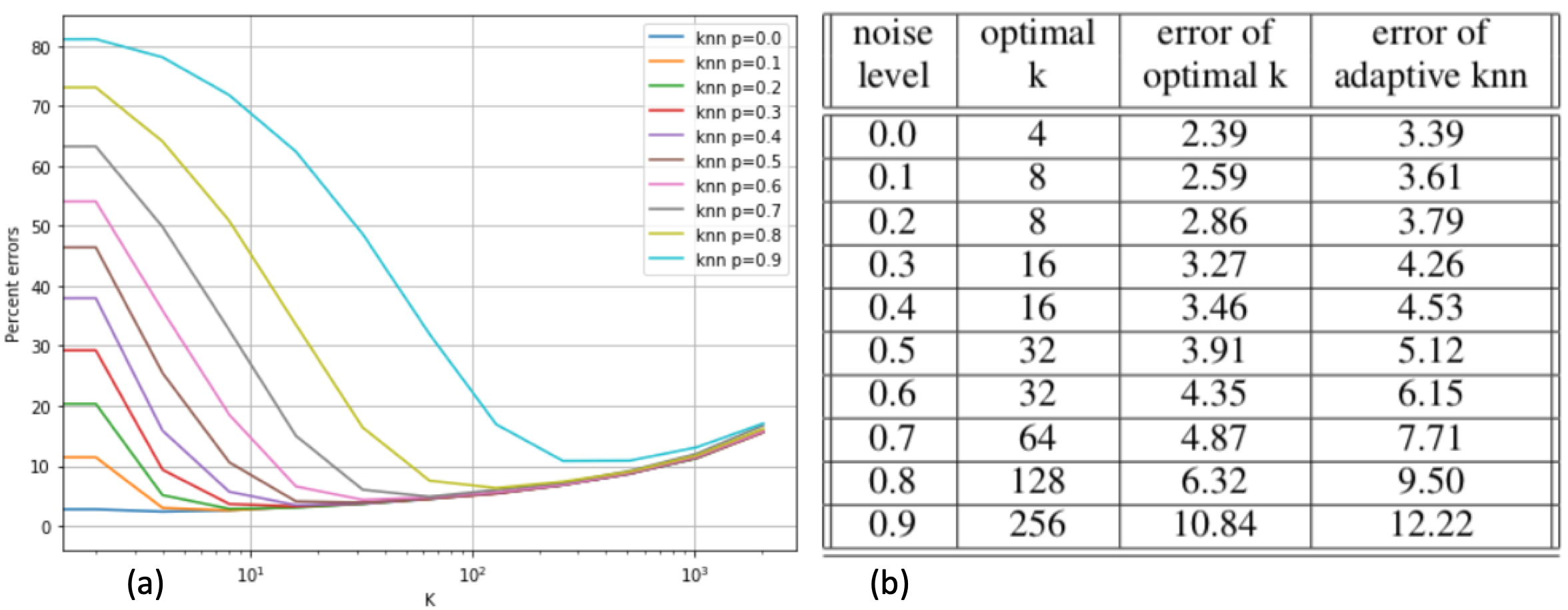
Figure 3: Effect of label noise on kπ‘˜k-NN and AKNN. Performance on MNIST for different levels of random label noise p𝑝p and for different values of kπ‘˜k. Each line in the figure on the left (a) represents the performance of kπ‘˜k-NN as a function of kπ‘˜k for a given level of noise. The optimal choice of kπ‘˜k increases with the noise level, and that the performance degrades severely for too-small kπ‘˜k. The table (b) shows that AKNN, with a fixed value of A𝐴A, performs almost as well as kπ‘˜k-NN with the optimal choice of kπ‘˜k.
Refer to caption

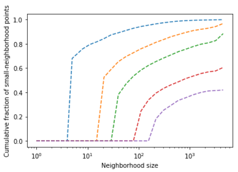
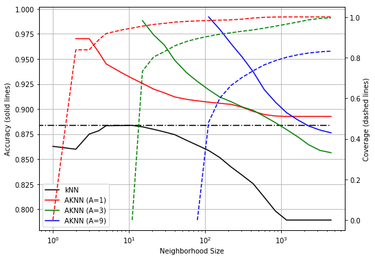
At left: performance of AKNN on notMNIST for different settings of the confidence parameter (A=1,3,9𝐴139A=1,3,9), as a function of the neighborhood size. For each confidence level we show two graphs: an accuracy graph (solid line) and a coverage line (dashed line). For each value of kπ‘˜k we plot the accuracy and the coverage of AKNN which is restricted to using a neighborhood size of at most kπ‘˜k. Increasing A𝐴A generally causes an increase in the accuracy and a decrease in coverage. Larger values of A𝐴A cause AKNN to have coverage zero for values of kπ‘˜k that are too small. For comparison, we plot the performance of kπ‘˜k-NN as a function of kπ‘˜k. The highest accuracy (β‰ˆ\approx 0.88) is achieved for k=10π‘˜10k=10 (dotted horizontal line), and is surpassed by AKNN with high coverage (100% for A=1𝐴1A=1).


Figure 4: Performance of AKNN on notMNIST. See also Figure 5.

6 Experiments

We performed a few experiments using real-world datasets from computer vision and genomics (see Section C). These were conducted with some practical alterations to the algorithm of Fig.Β 2.

Multiclass extension: Suppose the set of possible labels is 𝒴𝒴\mathcal{Y}. We replace the binary rule β€œfind the smallest kπ‘˜k such that |Ξ·n​(Bk​(x))|>Δ​(n,k,Ξ΄)subscriptπœ‚π‘›subscriptπ΅π‘˜π‘₯Ξ”π‘›π‘˜π›Ώ\left|\eta_{n}(B_{k}(x))\right|>\Delta(n,k,\delta)" with the rule: β€œfind the smallest kπ‘˜k such that Ξ·ny​(Bk​(x))βˆ’1|𝒴|>Δ​(n,k,Ξ΄)subscriptsuperscriptπœ‚π‘¦π‘›subscriptπ΅π‘˜π‘₯1π’΄Ξ”π‘›π‘˜π›Ώ\eta^{y}_{n}(B_{k}(x))-\frac{1}{|\mathcal{Y}|}>\Delta(n,k,\delta) for some yβˆˆπ’΄π‘¦π’΄y\in\mathcal{Y}, where Ξ·ny​(S)≐#n​{xi∈S​ and ​yi=y}#n​(S)approaches-limitsubscriptsuperscriptπœ‚π‘¦π‘›π‘†subscript#𝑛subscriptπ‘₯𝑖𝑆 andΒ subscript𝑦𝑖𝑦subscript#𝑛𝑆\eta^{y}_{n}(S)\doteq\frac{\#_{n}\{x_{i}\in S\mbox{ and }y_{i}=y\}}{\#_{n}(S)}."
Parametrization: We replace EquationΒ (6) with Ξ”=AkΞ”π΄π‘˜\Delta=\frac{A}{\sqrt{k}}, where A𝐴A is a confidence parameter corresponding to the theory’s δ𝛿\delta (given n𝑛n).
Resolving multilabel predictions: Our algorithm can output answers that are not a single label. The output can be β€œ?”, which indicates that no label has sufficient evidence. It can also be a subset of 𝒴𝒴\mathcal{Y} that contains more than one element, indicating that more than one label has significant evidence. In some situations, using subsets of the labels is more informative. However, when we want to compare head-to-head with kπ‘˜k-NN, we need to output a single label. We use a heuristic to predict with a single label yβˆˆπ’΄π‘¦π’΄y\in\mathcal{Y} on any xπ‘₯x: the label for which maxk⁑ηny​(Bk​(x))/ksubscriptπ‘˜subscriptsuperscriptπœ‚π‘¦π‘›subscriptπ΅π‘˜π‘₯π‘˜\max_{k}\eta^{y}_{n}(B_{k}(x))/\sqrt{k} is largest.

Refer to caption
Refer to caption
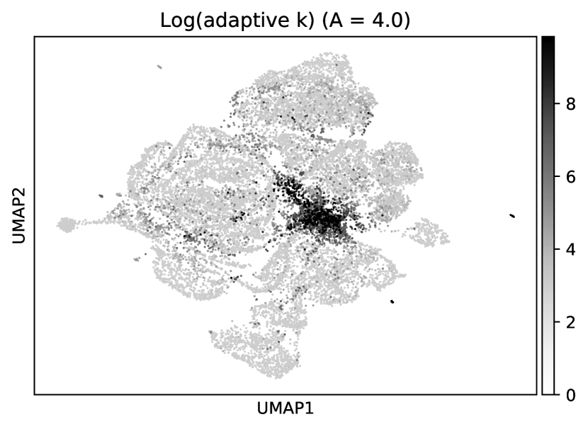
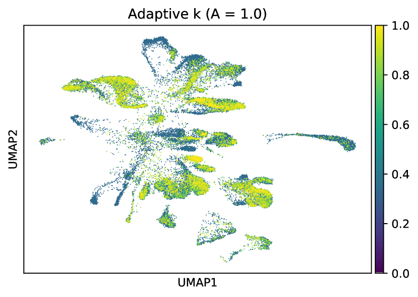
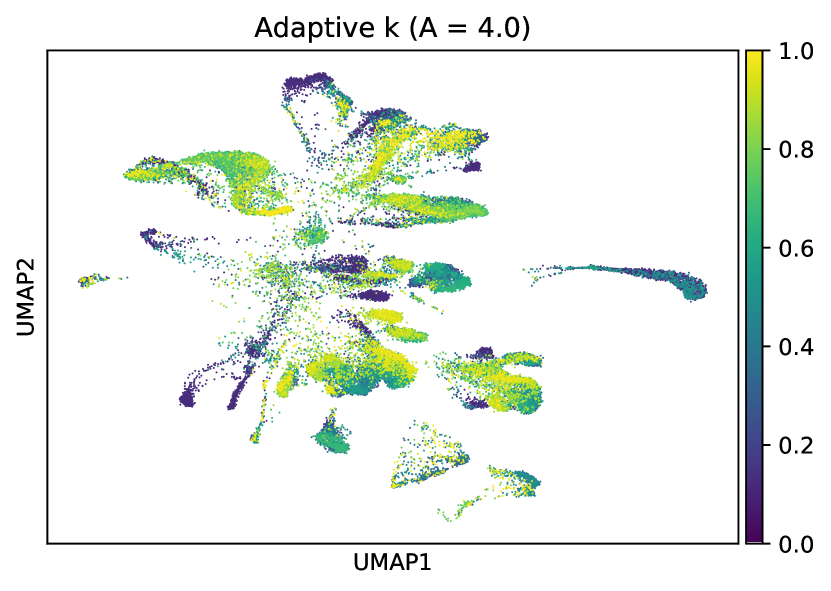
Figure 5: A visualization of the performance of AKNN on notMNIST. (a) The correct labels, with prediction errors of AKNN​(A=4)AKNN𝐴4\textsc{AKNN}\;(A=4) highlighted. (b) The value of kπ‘˜k chosen by the algorithm when predicting each datapoint. Zooming in reveals more details. An interactive explorer for our experiments is available at http://35.239.251.24/aknn/.

We briefly discuss our main conclusions from the experiments, with further details deferred to AppendixΒ C.

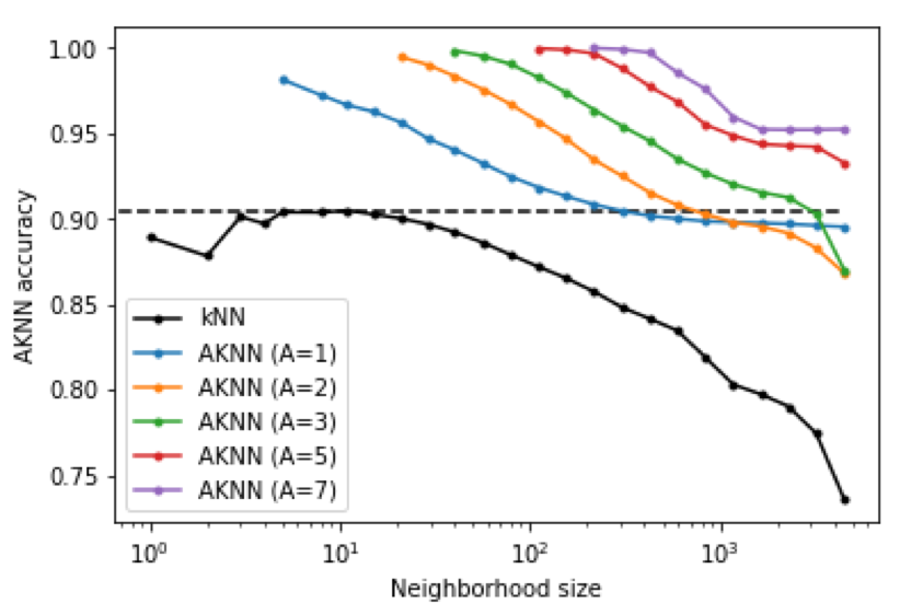
AKNN is comparable to the best kπ‘˜k-NN rule. In SectionΒ 4.2 we prove that AKNN compares favorably to kπ‘˜k-NN with any fixed kπ‘˜k. We demonstrate this in practice in different situations. With simulated independent label noise on the MNIST dataset (Fig.Β 3), a small value of kπ‘˜k is optimal for noiseless data, but performs very poorly when the noise level is high. On the other hand, AKNN adapts to the local noise level automatically, as demonstrated without adding noise on the more challenging notMNIST and single-cell genomics data (Fig. 4, 5, 6).

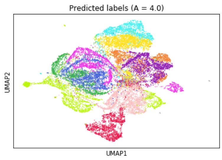
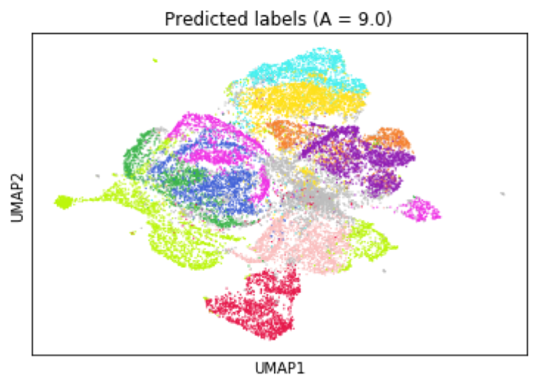
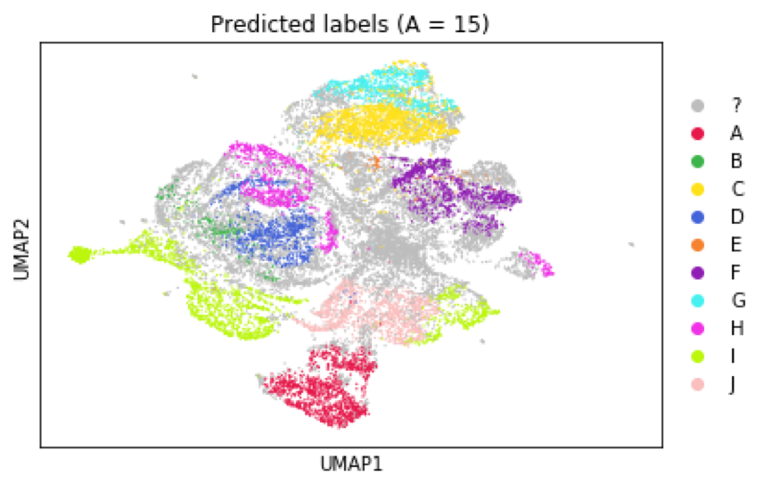
Varying the confidence parameter A𝐴A controls abstaining. The parameter A𝐴A controls how conservative the algorithm is in deciding to abstain, instead of incurring error by predicting. Aβ†’0→𝐴0A\to 0 represents the most aggressive setting, in which the algorithm never abstains, essentially predicting according to a 111-NN rule. Higher settings of A𝐴A cause the algorithm to abstain on some of these predicted points, for which there is no sufficiently small neighborhood with a sufficiently significant label bias (Fig. 7).

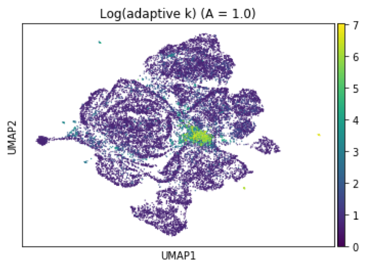
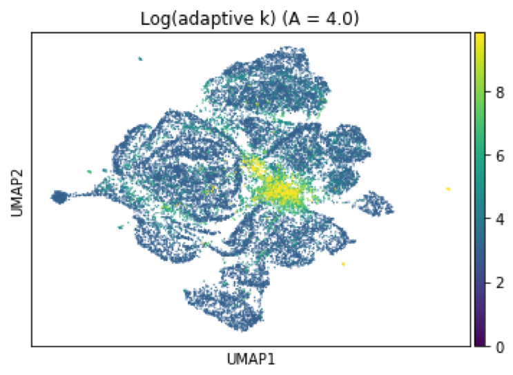
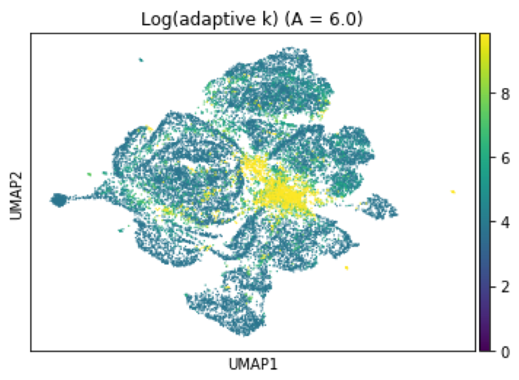
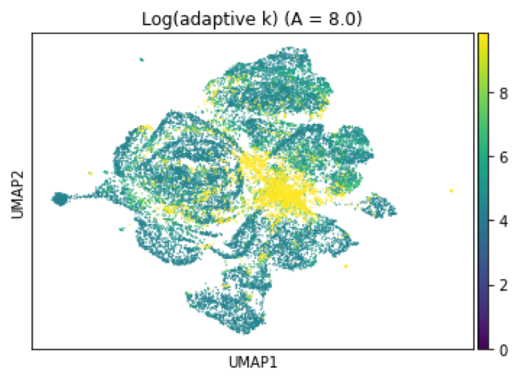
Adaptively chosen neighborhood sizes reflect local confidence. The number of neighbors chosen by AKNN is a local quantity that gives a practical pointwise measure of the confidence associated with label predictions. Small neighborhoods are chosen when one label is measured as significant nearly as soon as statistically possible; by definition of the AKNN stopping rule, this is not true where large neighborhoods are necessary. In our experiments, performance on points with significantly higher neighborhood sizes dropped monotonically, with the majority of the dataset having performance significantly exceeding the best kπ‘˜k-NN rule over a range of settings of A𝐴A (Fig. 4, 6; AppendixΒ C).

References

  • [AT07] J.-Y. Audibert and A.B. Tsybakov. Fast learning rates for plug-in classifiers. Annals of Statistics, 35(2):608–633, 2007.
  • [BBL05] StΓ©phane Boucheron, Olivier Bousquet, and GΓ‘bor Lugosi. Theory of classification: A survey of some recent advances. ESAIM: probability and statistics, 9:323–375, 2005.
  • [C+18] TabulaΒ Muris Consortium etΒ al. Single-cell transcriptomics of 20 mouse organs creates a tabula muris. Nature, 562(7727):367, 2018.
  • [CD10] K.Β Chaudhuri and S.Β Dasgupta. Rates of convergence for the cluster tree. In Advances in Neural Information Processing Systems, pages 343–351, 2010.
  • [CD14] K.Β Chaudhuri and S.Β Dasgupta. Rates of convergence for nearest neighbor classification. In Advances in Neural Information Processing Systems, pages 3437–3445. 2014.
  • [CG06] F.Β Cerou and A.Β Guyader. Nearest neighbor classification in infinite dimension. ESAIM: Probability and Statistics, 10:340–355, 2006.
  • [CH67] T.Β Cover and P.E. Hart. Nearest neighbor pattern classification. IEEE Transactions on Information Theory, 13:21–27, 1967.
  • [DCL11] Wei Dong, Moses Charikar, and Kai Li. Efficient k-nearest neighbor graph construction for generic similarity measures. In Proceedings of the 20th international conference on World wide web, pages 577–586. ACM, 2011.
  • [DGKL94] L.Β Devroye, L.Β GyΓΆrfi, A.Β Krzyzak, and G.Β Lugosi. On the strong universal consistency of nearest neighbor regression function estimates. Annals of Statistics, 22:1371–1385, 1994.
  • [DGL96] L.Β Devroye, L.Β GyΓΆrfi, and G.Β Lugosi. A Probabilistic Theory of Pattern Recognition. Springer, 1996.
  • [Dud79] R.M. Dudley. Balls in ℝksuperscriptβ„π‘˜\mathbb{R}^{k} do not cut all subsets of k+2π‘˜2k+2 points. Advances in Mathematics, 31(3):306–308, 1979.
  • [FH51] E.Β Fix and J.Β Hodges. Discriminatory analysis, nonparametric discrimination. USAF School of Aviation Medicine, Randolph Field, Texas, Project 21-49-004, Report 4, Contract AD41(128)-31, 1951.
  • [GyΓΆ81] L.Β GyΓΆrfi. The rate of convergence of knsubscriptπ‘˜π‘›k_{n}-nn regression estimates and classification rules. IEEE Transactions on Information Theory, 27(3):362–364, 1981.
  • [Hei01] J.Β Heinonen. Lectures on Analysis on Metric Spaces. Springer, 2001.
  • [KP95] S.Β Kulkarni and S.Β Posner. Rates of convergence of nearest neighbor estimation under arbitrary sampling. IEEE Transactions on Information Theory, 41(4):1028–1039, 1995.
  • [MNI]
  • [Mou18] Mouse cell atlas dataset. ftp://ngs.sanger.ac.uk/production/teichmann/BBKNN/MouseAtlas.zip, 2018. Accessed: 2019-05-02.
  • [MT99] E.Β Mammen and A.B. Tsybakov. Smooth discrimination analysis. The Annals of Statistics, 27(6):1808–1829, 1999.
  • [not11] notmnist dataset. http://yaroslavvb.com/upload/notMNIST/, 2011. Accessed: 2019-05-02.
  • [RS98] Martin Raab and Angelika Steger. "balls into bins" - A simple and tight analysis. In Randomization and Approximation Techniques in Computer Science, Second International Workshop, RANDOM’98, Barcelona, Spain, October 8-10, 1998, Proceedings, pages 159–170, 1998.
  • [Sto77] C.Β Stone. Consistent nonparametric regression. Annals of Statistics, 5:595–645, 1977.
  • [VC71] VladimirΒ N Vapnik and AΒ Ya Chervonenkis. On the uniform convergence of relative frequencies of events to their probabilities. Theory of Probability & Its Applications, 16(2):264–280, 1971.

Appendix A Analysis and proofs

The first step in establishing advantage-dependent rates of convergence is to bound the accuracy of empirical estimates of probability mass and bias. This is achieved by a careful choice of large deviation bounds.

A.1 Large deviation bounds

Suppose we draw n𝑛n points (x1,y1),…,(xn,yn)subscriptπ‘₯1subscript𝑦1…subscriptπ‘₯𝑛subscript𝑦𝑛(x_{1},y_{1}),\ldots,(x_{n},y_{n}) from P𝑃P. If n𝑛n is reasonably large, we would expect the empirical mass ΞΌn​(S)subscriptπœ‡π‘›π‘†\mu_{n}(S) of any set SβŠ‚π’³π‘†π’³S\subset{\mathcal{X}}, as defined in (4), to be close to its probability mass under ΞΌπœ‡\mu. The following lemma, from [CD10], quantifies one particular aspect of this.

Lemma 5 ([CD10], Lemma 7).

There is a universal constant cosubscriptπ‘π‘œc_{o} such that the following holds. Let ℬℬ{\mathcal{B}} be any class of measurable subsets of 𝒳𝒳{\mathcal{X}} of VC dimension d0subscript𝑑0d_{0}. Pick any 0<Ξ΄<10𝛿10<\delta<1. Then with probability at least 1βˆ’Ξ΄2/21superscript𝛿221-\delta^{2}/2 over the choice of (x1,y1),…,(xn,yn)subscriptπ‘₯1subscript𝑦1…subscriptπ‘₯𝑛subscript𝑦𝑛(x_{1},y_{1}),\ldots,(x_{n},y_{n}), for all Bβˆˆβ„¬π΅β„¬B\in{\mathcal{B}} and for any integer kπ‘˜k, we have

μ​(B)β‰₯kn+con​max⁑(k,d0​log⁑nΞ΄)⟹μn​(B)β‰₯kn.formulae-sequenceπœ‡π΅π‘˜π‘›subscriptπ‘π‘œπ‘›π‘˜subscript𝑑0𝑛𝛿subscriptπœ‡π‘›π΅π‘˜π‘›\mu(B)\geq\frac{k}{n}+\frac{c_{o}}{n}\max\left(k,d_{0}\log\frac{n}{\delta}\right)\ \ \implies\ \ \mu_{n}(B)\geq\frac{k}{n}.

Likewise, we would expect the empirical bias Ξ·n​(S)subscriptπœ‚π‘›π‘†\eta_{n}(S) of a set SβŠ‚π’³π‘†π’³S\subset{\mathcal{X}}, as defined in (5), to be close to its true bias η​(S)πœ‚π‘†\eta(S). The latter is defined whenever μ​(S)>0πœ‡π‘†0\mu(S)>0.

Lemma 6.

There is a universal constant c1subscript𝑐1c_{1} for which the following holds. Let π’žπ’ž\mathcal{C} be a class of subsets of 𝒳𝒳{\mathcal{X}} with VC dimension d0subscript𝑑0d_{0}. Pick any 0<Ξ΄<10𝛿10<\delta<1. Then with probability at least 1βˆ’Ξ΄2/21superscript𝛿221-\delta^{2}/2 over the choice of (x1,y1),…,(xn,yn)subscriptπ‘₯1subscript𝑦1…subscriptπ‘₯𝑛subscript𝑦𝑛(x_{1},y_{1}),\ldots,(x_{n},y_{n}), for all Cβˆˆπ’žπΆπ’žC\in\mathcal{C},

|Ξ·n​(C)βˆ’Ξ·β€‹(C)|≀Δ​(n,#n​(C),Ξ΄)subscriptπœ‚π‘›πΆπœ‚πΆΞ”π‘›subscript#𝑛𝐢𝛿\left|\eta_{n}(C)-\eta(C)\right|\ \leq\ \Delta(n,\#_{n}(C),\delta)

where #n​(C)=|{i:xi∈B}|subscript#𝑛𝐢conditional-set𝑖subscriptπ‘₯𝑖𝐡\#_{n}(C)=|\{i:x_{i}\in B\}| is the number of points in C𝐢C and

Δ​(n,k,Ξ΄)=c1​d0​log⁑n+log⁑(1/Ξ΄)k.Ξ”π‘›π‘˜π›Ώsubscript𝑐1subscript𝑑0𝑛1π›Ώπ‘˜\Delta(n,k,\delta)=c_{1}\sqrt{\frac{d_{0}\log n+\log(1/\delta)}{k}}. (11)

EquationΒ 11 is a special case222Indeed, EquationΒ 11 follows from TheoremΒ 8 by plugging in it π’œ={𝒳×{+1}},ℬ={CΓ—{Β±1}:Cβˆˆπ’ž}formulae-sequenceπ’œπ’³1ℬconditional-set𝐢plus-or-minus1πΆπ’ž\mathcal{A}=\{{\mathcal{X}}\times\{+1\}\},{\mathcal{B}}=\{C\times\{\pm 1\}:C\in\mathcal{C}\}. of a uniform convergence bound for conditional probabilities (TheoremΒ 8) that we present and prove in AppendixΒ B.

A.2 Proof of TheoremΒ 1

Theorem (TheoremΒ 1 restatement).

There is an absolute constant C>0𝐢0C>0 for which the following holds. Let 0<Ξ΄<10𝛿10<\delta<1 denote the confidence parameter in the AKNN algorithm (FigureΒ 2), and suppose the algorithm is used to define a classifier gnsubscript𝑔𝑛g_{n} based on n𝑛n training points chosen i.i.d.Β from P𝑃P. Then, for every point x∈supp​(ΞΌ)π‘₯suppπœ‡x\in{\rm supp}(\mu), if

nβ‰₯Cadv​(x)​max⁑(log⁑1adv​(x),log⁑1Ξ΄)𝑛𝐢advπ‘₯1advπ‘₯1𝛿n\geq\frac{C}{{\rm adv}(x)}\max\left(\log\frac{1}{{\rm adv}(x)},\ \log\frac{1}{\delta}\right)

then with probability at least 1βˆ’Ξ΄1𝛿1-\delta we have that gn​(x)=gβˆ—β€‹(x)subscript𝑔𝑛π‘₯superscript𝑔π‘₯g_{n}(x)=g^{*}(x).

Proof.

Define c2=max⁑(c1,1/2)​1+cosubscript𝑐2subscript𝑐1121subscriptπ‘π‘œc_{2}=\max(c_{1},1/2)\sqrt{1+c_{o}}, where cosubscriptπ‘π‘œc_{o} and c1subscript𝑐1c_{1} are the constants from LemmasΒ 5 and 11, and take c3=16​c22subscript𝑐316superscriptsubscript𝑐22c_{3}=16c_{2}^{2}.

Suppose η​(x)>0πœ‚π‘₯0\eta(x)>0; the negative case is symmetric. The set ℬℬ{\mathcal{B}} of all balls centered at xπ‘₯x is easily seen to have VC dimension d0=1subscript𝑑01d_{0}=1. By LemmasΒ 5 and 11, we have that with probability at least 1βˆ’Ξ΄21superscript𝛿21-\delta^{2}, the following two properties hold for all Bβˆˆβ„¬π΅β„¬B\in{\mathcal{B}}:

  1. 1.

    For any integer kπ‘˜k, we have #n​(B)β‰₯ksubscript#π‘›π΅π‘˜\#_{n}(B)\geq k whenever n​μ​(B)β‰₯k+co​max⁑(k,log⁑(n/Ξ΄))π‘›πœ‡π΅π‘˜subscriptπ‘π‘œπ‘˜π‘›π›Ώn\mu(B)\geq k+c_{o}\max(k,\log(n/\delta)).

  2. 2.

    |Ξ·n​(B)βˆ’Ξ·β€‹(B)|≀Δ​(n,#n​(B),Ξ΄)subscriptπœ‚π‘›π΅πœ‚π΅Ξ”π‘›subscript#𝑛𝐡𝛿|\eta_{n}(B)-\eta(B)|\leq\Delta(n,\#_{n}(B),\delta).

Assume henceforth that these hold.

By the definition of advantage, point xπ‘₯x is (p,Ξ³)𝑝𝛾(p,\gamma)-salient for some p,Ξ³>0𝑝𝛾0p,\gamma>0 with adv​(x)=p​γ2advπ‘₯𝑝superscript𝛾2{\rm adv}(x)=p\gamma^{2}. The lower bound on n𝑛n in the theorem statement implies that

Ξ³β‰₯2​c2​log⁑n+log⁑(1/Ξ΄)n​p,𝛾2subscript𝑐2𝑛1𝛿𝑛𝑝\gamma\geq 2c_{2}\sqrt{\frac{\log n+\log(1/\delta)}{np}}, (12)

or equivalently that nβ‹…adv​(x)β‰₯4​c22​(log⁑n+log⁑(1/Ξ΄))⋅𝑛advπ‘₯4superscriptsubscript𝑐22𝑛1𝛿n\cdot{\rm adv}(x)\geq 4c_{2}^{2}(\log n+\log(1/\delta)).

Set k=n​p/(1+w)π‘˜π‘›π‘1𝑀k=np/(1+w). By (12) we have n​pβ‰₯4​c22​log⁑(n/Ξ΄)𝑛𝑝4superscriptsubscript𝑐22𝑛𝛿np\geq 4c_{2}^{2}\log(n/\delta) and thus kβ‰₯log⁑(n/Ξ΄)π‘˜π‘›π›Ώk\geq\log(n/\delta). As a result, n​pβ‰₯k+w​max⁑(k,log⁑(n/Ξ΄))π‘›π‘π‘˜π‘€π‘˜π‘›π›Ώnp\geq k+w\max(k,\log(n/\delta)), and by property 1, the ball B=B​(x,rp​(x))𝐡𝐡π‘₯subscriptπ‘Ÿπ‘π‘₯B=B(x,r_{p}(x)) has #n​(B)β‰₯ksubscript#π‘›π΅π‘˜\#_{n}(B)\geq k. This means, in turn, that by property 2,

Ξ·n​(B)subscriptπœ‚π‘›π΅\displaystyle\eta_{n}(B) β‰₯η​(B)βˆ’Ξ”β€‹(n,k,Ξ΄)=Ξ³βˆ’c1​log⁑(n/Ξ΄)kabsentπœ‚π΅Ξ”π‘›π‘˜π›Ώπ›Ύsubscript𝑐1π‘›π›Ώπ‘˜\displaystyle\geq\ \eta(B)-\Delta(n,k,\delta)=\gamma-c_{1}\sqrt{\frac{\log(n/\delta)}{k}}
β‰₯2​c2​log⁑(n/Ξ΄)n​pβˆ’c1​log⁑(n/Ξ΄)kβ‰₯2​c1​log⁑(n/Ξ΄)kβˆ’c1​log⁑(n/Ξ΄)kabsent2subscript𝑐2𝑛𝛿𝑛𝑝subscript𝑐1π‘›π›Ώπ‘˜2subscript𝑐1π‘›π›Ώπ‘˜subscript𝑐1π‘›π›Ώπ‘˜\displaystyle\geq 2c_{2}\sqrt{\frac{\log(n/\delta)}{np}}-c_{1}\sqrt{\frac{\log(n/\delta)}{k}}\geq 2c_{1}\sqrt{\frac{\log(n/\delta)}{k}}-c_{1}\sqrt{\frac{\log(n/\delta)}{k}}
=c1​log⁑(n/Ξ΄)kβ‰₯Δ​(n,#n​(B),Ξ΄).absentsubscript𝑐1π‘›π›Ώπ‘˜Ξ”π‘›subscript#𝑛𝐡𝛿\displaystyle=c_{1}\sqrt{\frac{\log(n/\delta)}{k}}\geq\Delta(n,\#_{n}(B),\delta).

Thus ball B𝐡B would trigger a prediction of +11+1.

At the same time, for any ball Bβ€²=B​(x,r)superscript𝐡′𝐡π‘₯π‘ŸB^{\prime}=B(x,r) with r<rp​(x)π‘Ÿsubscriptπ‘Ÿπ‘π‘₯r<r_{p}(x),

Ξ·n​(Bβ€²)β‰₯η​(Bβ€²)βˆ’Ξ”β€‹(n,#n​(Bβ€²),Ξ΄)>βˆ’Ξ”β€‹(n,#n​(Bβ€²),Ξ΄)subscriptπœ‚π‘›superscriptπ΅β€²πœ‚superscript𝐡′Δ𝑛subscript#𝑛superscript𝐡′𝛿Δ𝑛subscript#𝑛superscript𝐡′𝛿\eta_{n}(B^{\prime})\geq\eta(B^{\prime})-\Delta(n,\#_{n}(B^{\prime}),\delta)>-\Delta(n,\#_{n}(B^{\prime}),\delta)

and thus no such ball will trigger a prediction of βˆ’11-1. Therefore, the prediction at xπ‘₯x must be +11+1. ∎

A.3 Proof of TheoremΒ 2

This proof follows much the same outline as that of TheoremΒ 1. A crucial difference is that uniform large deviation bounds (LemmasΒ 5 and 11) are applied to the class of all balls in 𝒳𝒳{\mathcal{X}}, which is assumed333This is motivated by finite-dimensional Euclidean space ℝDsuperscriptℝ𝐷\mathbb{R}^{D}, where it holds with d0=D+1subscript𝑑0𝐷1d_{0}=D+1 ([Dud79]). to have finite VC dimension d0subscript𝑑0d_{0}. In contrast, the proof of TheoremΒ 1 only applies these bounds to the class of balls centered at a specific point, which has VC dimension at most 1 in any metric space.

A.4 Proof of TheoremΒ 4

Recall from (9) that 𝒳asubscriptπ’³π‘Ž{\mathcal{X}}_{a} denotes the set of points with advantage >aabsentπ‘Ž>a.

Lemma 7.

Pick any 0<Ξ΄<10𝛿10<\delta<1 as a confidence parameter for the AKNN estimator of FigureΒ 2. Fix any a>0π‘Ž0a>0. If the number of training points n𝑛n satisfies

nβ‰₯c3a​max⁑(log⁑c3a,log⁑1Ξ΄),𝑛subscript𝑐3π‘Žsubscript𝑐3π‘Ž1𝛿n\geq\frac{c_{3}}{a}\max\left(\log\frac{c_{3}}{a},\ \log\frac{1}{\delta}\right),

then with probability at least 1βˆ’Ξ΄1𝛿1-\delta, the resulting classifier gnsubscript𝑔𝑛g_{n} has risk

R​(gn)βˆ’Rβˆ—β‰€Ξ΄+μ​(𝒳0βˆ–π’³a).𝑅subscript𝑔𝑛superscriptπ‘…π›Ώπœ‡subscript𝒳0subscriptπ’³π‘ŽR(g_{n})-R^{*}\leq\delta+\mu({\mathcal{X}}_{0}\setminus{\mathcal{X}}_{a}).
Proof.

From TheoremΒ 1 , we have that for any xβˆˆπ’³aπ‘₯subscriptπ’³π‘Žx\in{\mathcal{X}}_{a},

Prn​(gn​(x)β‰ gβˆ—β€‹(x))≀δ2,subscriptPr𝑛subscript𝑔𝑛π‘₯superscript𝑔π‘₯superscript𝛿2{\rm Pr}_{n}(g_{n}(x)\neq g^{*}(x))\leq\delta^{2},

where PrnsubscriptPr𝑛{\rm Pr}_{n} denotes probability over the choice of training points. Thus, for X∼μsimilar-toπ‘‹πœ‡X\sim\mu,

𝔼n​𝔼X​1​(gn​(X)β‰ gβˆ—β€‹(X)|Xβˆˆπ’³a)≀δ2,subscript𝔼𝑛subscript𝔼𝑋1subscript𝑔𝑛𝑋conditionalsuperscript𝑔𝑋𝑋subscriptπ’³π‘Žsuperscript𝛿2{\mathbb{E}}_{n}{\mathbb{E}}_{X}1(g_{n}(X)\neq g^{*}(X)|X\in{\mathcal{X}}_{a})\leq\delta^{2},

and by Markov’s inequality,

Prn​[PrX​(gn​(X)β‰ gβˆ—β€‹(X)|Xβˆˆπ’³a)β‰₯Ξ΄]≀δ.subscriptPr𝑛delimited-[]subscriptPr𝑋subscript𝑔𝑛𝑋conditionalsuperscript𝑔𝑋𝑋subscriptπ’³π‘Žπ›Ώπ›Ώ{\rm Pr}_{n}[{\rm Pr}_{X}(g_{n}(X)\neq g^{*}(X)|X\in{\mathcal{X}}_{a})\geq\delta]\leq\delta.

Thus, with probability at least 1βˆ’Ξ΄1𝛿1-\delta over the training set,

PrX​(gn​(X)β‰ gβˆ—β€‹(X)|Xβˆˆπ’³a)≀δ.subscriptPr𝑋subscript𝑔𝑛𝑋conditionalsuperscript𝑔𝑋𝑋subscriptπ’³π‘Žπ›Ώ{\rm Pr}_{X}(g_{n}(X)\neq g^{*}(X)|X\in{\mathcal{X}}_{a})\leq\delta.

On points with η​(x)=0πœ‚π‘₯0\eta(x)=0, both gnsubscript𝑔𝑛g_{n} and the Bayes-optimal gβˆ—superscript𝑔g^{*} incur the same risk. Thus

R​(gn)βˆ’Rβˆ—π‘…subscript𝑔𝑛superscript𝑅\displaystyle R(g_{n})-R^{*} ≀PrX​(gn​(X)β‰ gβˆ—β€‹(X)|Xβˆˆπ’³a)+PrX​(Xβˆ‰π’³a,η​(X)β‰ 0)absentsubscriptPr𝑋subscript𝑔𝑛𝑋conditionalsuperscript𝑔𝑋𝑋subscriptπ’³π‘ŽsubscriptPr𝑋formulae-sequence𝑋subscriptπ’³π‘Žπœ‚π‘‹0\displaystyle\leq{\rm Pr}_{X}(g_{n}(X)\neq g^{*}(X)|X\in{\mathcal{X}}_{a})+{\rm Pr}_{X}(X\not\in{\mathcal{X}}_{a},\eta(X)\neq 0)
≀δ+PrX​(Xβˆˆπ’³0βˆ–π’³a)+PrX​(adv​(X)=0,η​(X)β‰ 0)absent𝛿subscriptPr𝑋𝑋subscript𝒳0subscriptπ’³π‘ŽsubscriptPr𝑋formulae-sequenceadv𝑋0πœ‚π‘‹0\displaystyle\leq\delta+{\rm Pr}_{X}(X\in{\mathcal{X}}_{0}\setminus{\mathcal{X}}_{a})+{\rm Pr}_{X}({\rm adv}(X)=0,\eta(X)\neq 0)
≀δ+μ​(𝒳0βˆ–π’³a),absentπ›Ώπœ‡subscript𝒳0subscriptπ’³π‘Ž\displaystyle\leq\delta+\mu({\mathcal{X}}_{0}\setminus{\mathcal{X}}_{a}),

where we invoke Lemma 3 for the last step. ∎

We now complete the proof of TheoremΒ 4. Given the sequence of confidence parameters (Ξ΄n)subscript𝛿𝑛(\delta_{n}), define a sequence of advantage values (an)subscriptπ‘Žπ‘›(a_{n}) by

an=c3n​max⁑(2​log⁑n,log⁑1Ξ΄n).subscriptπ‘Žπ‘›subscript𝑐3𝑛2𝑛1subscript𝛿𝑛a_{n}=\frac{c_{3}}{n}\max\left(2\log n,\ \log\frac{1}{\delta_{n}}\right).

The conditions on (Ξ΄n)subscript𝛿𝑛(\delta_{n}) imply anβ†’0β†’subscriptπ‘Žπ‘›0a_{n}\rightarrow 0.

Pick any Ο΅>0italic-Ο΅0\epsilon>0. By the conditions on (Ξ΄n)subscript𝛿𝑛(\delta_{n}), we can pick N𝑁N so that βˆ‘nβ‰₯NΞ΄n≀ϡsubscript𝑛𝑁subscript𝛿𝑛italic-Ο΅\sum_{n\geq N}\delta_{n}\leq\epsilon. Let Ο‰πœ”\omega denote a realization of an infinite training sequence (X1,Y1),(X2,Y2),…subscript𝑋1subscriptπ‘Œ1subscript𝑋2subscriptπ‘Œ2…(X_{1},Y_{1}),(X_{2},Y_{2}),\ldots from P𝑃P. By LemmaΒ 7, for any positive integer N𝑁N,

Pr(Ο‰:βˆƒnβ‰₯NΒ s.t.Β R(gn(Ο‰))βˆ’Rβˆ—>Ξ΄n+ΞΌ(𝒳0βˆ–π’³an))β‰€βˆ‘nβ‰₯NΞ΄n≀ϡ.{\rm Pr}\left(\omega:\exists n\geq N\mbox{\ s.t.\ }R(g_{n}(\omega))-R^{*}>\delta_{n}+\mu({\mathcal{X}}_{0}\setminus{\mathcal{X}}_{a_{n}})\right)\leq\sum_{n\geq N}\delta_{n}\leq\epsilon.

Thus, with probability at least 1βˆ’Ο΅1italic-Ο΅1-\epsilon over the training sequence Ο‰πœ”\omega, we have that for all nβ‰₯N𝑛𝑁n\geq N,

R​(gn​(Ο‰))βˆ’Rβˆ—β‰€Ξ΄n+μ​(𝒳0βˆ–π’³an),𝑅subscriptπ‘”π‘›πœ”superscript𝑅subscriptπ›Ώπ‘›πœ‡subscript𝒳0subscript𝒳subscriptπ‘Žπ‘›R(g_{n}(\omega))-R^{*}\leq\delta_{n}+\mu({\mathcal{X}}_{0}\setminus{\mathcal{X}}_{a_{n}}),

whereupon R​(gn​(Ο‰))β†’Rβˆ—β†’π‘…subscriptπ‘”π‘›πœ”superscript𝑅R(g_{n}(\omega))\rightarrow R^{*} (since Ξ΄n,anβ†’0β†’subscript𝛿𝑛subscriptπ‘Žπ‘›0\delta_{n},a_{n}\rightarrow 0 and lima↓0μ​(𝒳0βˆ–π’³a)=0subscriptβ†“π‘Ž0πœ‡subscript𝒳0subscriptπ’³π‘Ž0\lim_{a\downarrow 0}\mu({\mathcal{X}}_{0}\setminus{\mathcal{X}}_{a})=0). Since this holds for any Ο΅>0italic-Ο΅0\epsilon>0, the theorem follows.

Appendix B Uniform Convergence of Empirical Conditional Measures

B.1 Formal Statement

Let P𝑃P be a distribution over X𝑋X, and let π’œ,β„¬π’œβ„¬\mathcal{A},\mathcal{B} be two collections of events. Consider n𝑛n independent samples fromΒ P𝑃P, denoted byΒ x1,…,xnsubscriptπ‘₯1…subscriptπ‘₯𝑛x_{1},\ldots,x_{n}. We would like to estimate P​(A|B)𝑃conditional𝐴𝐡P(A|B) simultaneously for allΒ Aβˆˆπ’œ,Bβˆˆβ„¬formulae-sequenceπ΄π’œπ΅β„¬A\in\mathcal{A},B\in\mathcal{B}. It is natural to consider the empirical estimates:

Pn​(A|B)=βˆ‘i1[xi∈A∩B]βˆ‘i1[xi∈B].subscript𝑃𝑛conditional𝐴𝐡subscript𝑖subscript1delimited-[]subscriptπ‘₯𝑖𝐴𝐡subscript𝑖subscript1delimited-[]subscriptπ‘₯𝑖𝐡P_{n}(A|B)=\frac{\sum_{i}1_{[x_{i}\in A\cap B]}}{\sum_{i}1_{[x_{i}\in B]}}.

We study when (and to what extent) these estimates provide a good approximation. Note that the case where ℬ={X}ℬ𝑋\mathcal{B}=\{X\} (i.e., in which one estimates P​(A)𝑃𝐴P(A) using Pn​(A)subscript𝑃𝑛𝐴P_{n}(A) simultaneously for all Aβˆˆπ’œπ΄π’œA\in\mathcal{A}) is handled by the classical VC theory. Throughout this section we assume that both π’œ,β„¬π’œβ„¬\mathcal{A},\mathcal{B} have a finite VC-dimension, and we let d0subscript𝑑0d_{0} denote an upper bound on both 𝖡𝖒​(π’œ)π–΅π–’π’œ\mathsf{VC}(\mathcal{A}) and 𝖡𝖒​(ℬ)𝖡𝖒ℬ\mathsf{VC}(\mathcal{B}).

To demonstrate the kinds of statements we would like to derive, consider the case where each ofΒ π’œ,β„¬π’œβ„¬\mathcal{A},\mathcal{B} contains only one event: π’œ={A}π’œπ΄\mathcal{A}=\{A\}, and ℬ={B}ℬ𝐡\mathcal{B}=\{B\}, and set #n​(B)=βˆ‘i1[xi∈B]subscript#𝑛𝐡subscript𝑖subscript1delimited-[]subscriptπ‘₯𝑖𝐡\#_{n}(B)=\sum_{i}1_{[x_{i}\in B]}. A Chernoff bound implies that conditioned on the event that #n​(B)>0subscript#𝑛𝐡0\#_{n}(B)>0, the following holds with probability at leastΒ 1βˆ’Ξ΄1𝛿1-\delta:

|P​(A|B)βˆ’Pn​(A|B)|≀2​log⁑(1/Ξ΄)#n​(B).𝑃conditional𝐴𝐡subscript𝑃𝑛conditional𝐴𝐡21𝛿subscript#𝑛𝐡\left\lvert P(A|B)-P_{n}(A|B)\right\rvert\leq\sqrt{\frac{2\log(1/\delta)}{\#_{n}(B)}}. (13)

To derive it, use that conditioned on xi∈Bsubscriptπ‘₯𝑖𝐡x_{i}\in B, the event xi∈Asubscriptπ‘₯𝑖𝐴x_{i}\in A has probability P​(A|B)𝑃conditional𝐴𝐡P(A|B), and therefore the random variable β€œ#n​(B)β‹…pn​(A|B)β‹…subscript#𝑛𝐡subscript𝑝𝑛conditional𝐴𝐡\#_{n}(B)\cdot p_{n}(A|B)” has a binomial distribution with parameters #n​(B)subscript#𝑛𝐡\#_{n}(B) and P​(A|B)𝑃conditional𝐴𝐡P(A|B).

Note that the bound on the error in EquationΒ 13 depends on #n​(B)subscript#𝑛𝐡\#_{n}(B) and therefore is data-dependent. We stress that this is the type of statement we want: the more samples belong to B𝐡B, the more certain we are with the empirical estimate. Thus, we would want to prove a statement as follows:

With probability at leastΒ 1βˆ’Ξ΄1𝛿1-\delta,

(βˆ€Aβˆˆπ’œ)​(βˆ€Bβˆˆβ„¬):|P​(A|B)βˆ’Pn​(A|B)|≀O​(d0​log⁑(1/Ξ΄)#n​(B)),:for-allπ΄π’œfor-all𝐡ℬ𝑃conditional𝐴𝐡subscript𝑃𝑛conditional𝐴𝐡𝑂subscript𝑑01𝛿subscript#𝑛𝐡\left(\forall A\in\mathcal{A}\right)\left(\forall B\in{\mathcal{B}}\right):\left\lvert P(A|B)-P_{n}(A|B)\right\rvert\leq O\left(\sqrt{\frac{d_{0}\log(1/\delta)}{\#_{n}(B)}}\right),

where #n​(B)=βˆ‘i=1n1​[xi∈B]subscript#𝑛𝐡superscriptsubscript𝑖1𝑛1delimited-[]subscriptπ‘₯𝑖𝐡\#_{n}(B)=\sum_{i=1}^{n}1[x_{i}\in B].

The above statement is, unfortunately, false. As an example, consider the probability space defined by drawing x∼[n]similar-toπ‘₯delimited-[]𝑛x\sim[n] uniformly, and then coloring xπ‘₯x by cx∈{Β±1}subscript𝑐π‘₯plus-or-minus1c_{x}\in\{\pm 1\} uniformly. For each i𝑖i let Bisubscript𝐡𝑖B_{i} denote the event thatΒ i𝑖i was drawn, and let A𝐴A denote the event that the drawn color was +11+1. (formally, Bi={i}Γ—{Β±1}subscript𝐡𝑖𝑖plus-or-minus1B_{i}=\{i\}\times\{\pm 1\}, and A=[n]Γ—{+1}𝐴delimited-[]𝑛1A=[n]\times\{+1\}). One can verify that the VC dimension of ℬ={Bi:i≀n}ℬconditional-setsubscript𝐡𝑖𝑖𝑛{\mathcal{B}}=\{B_{i}:i\leq n\} and of π’œ={A}π’œπ΄\mathcal{A}=\{A\} is at most 111. The above statement fails in this setting: indeed, one can verify that if we draw n𝑛n samples from this space then with a constant probability there will be some j𝑗j such that:

  • (i)

    j𝑗j always gets the same color (say +11+1), and

  • (ii)

    j𝑗j is sampled at least Ω​(log⁑n/log⁑log⁑n)Ω𝑛𝑛\Omega(\log n/\log\log n) times444This follows from analyzing the maximal bin in a uniform assignment of Ξ˜β€‹(n)Ξ˜π‘›\Theta(n) balls into n𝑛n binsΒ [RS98].

Therefore, with constant probability we get that

Pn​(A|Bi)=1,P​(A|Bi)=1/2,formulae-sequencesubscript𝑃𝑛conditional𝐴subscript𝐡𝑖1𝑃conditional𝐴subscript𝐡𝑖12P_{n}(A|B_{i})=1,P(A|B_{i})=1/2,

and so the difference between the error is clearly 1βˆ’(1/2)=1/2112121-(1/2)=1/2, which is clearly not upper bounded by O​(log⁑log⁑n/log⁑n)𝑂𝑛𝑛O(\sqrt{\log\log n/\log n}).

We prove the following (slightly weaker) variant:

Theorem 8 (UCECM).

Let P𝑃P be a probability distribution over X𝑋X, and let π’œ,β„¬π’œβ„¬\mathcal{A},\mathcal{B} be two families of measurable subsets of X𝑋X such that 𝖡𝖒​(π’œ),𝖡𝖒​(ℬ)≀d0π–΅π–’π’œπ–΅π–’β„¬subscript𝑑0\mathsf{VC}(\mathcal{A}),\mathsf{VC}(\mathcal{B})\leq d_{0}. Let nβˆˆβ„•π‘›β„•n\in\mathbb{N}, and let x1​…​xnsubscriptπ‘₯1…subscriptπ‘₯𝑛x_{1}\ldots x_{n} be n𝑛n i.i.d samples from P𝑃P. The, the following event occurs with probability at least 1βˆ’Ξ΄1𝛿1-\delta:

(βˆ€Aβˆˆπ’œ)​(βˆ€Bβˆˆβ„¬):|P​(A|B)βˆ’Pn​(A|B)|≀ko#n​(B),:for-allπ΄π’œfor-all𝐡ℬ𝑃conditional𝐴𝐡subscript𝑃𝑛conditional𝐴𝐡subscriptπ‘˜π‘œsubscript#𝑛𝐡\left(\forall A\in\mathcal{A}\right)\left(\forall B\in{\mathcal{B}}\right):\left\lvert P(A|B)-P_{n}(A|B)\right\rvert\leq\sqrt{\frac{k_{o}}{\#_{n}(B)}},

where ko=1000​(d0​log⁑(8​n)+log⁑(4/Ξ΄))subscriptπ‘˜π‘œ1000subscript𝑑08𝑛4𝛿k_{o}=1000\left(d_{0}\log(8n)+\log(4/\delta)\right), and555Note that the above inequality makes sense also when k​(B)=0π‘˜π΅0k(B)=0, by identifying β‹…0β‹…0\frac{\cdot}{0} as ∞\infty, and using the convention that βˆžβˆ’βˆž=∞\infty-\infty=\infty and that βˆžβ‰€βˆž\infty\leq\infty. #n​(B)=βˆ‘i=1n1​[xi∈B]subscript#𝑛𝐡superscriptsubscript𝑖1𝑛1delimited-[]subscriptπ‘₯𝑖𝐡\#_{n}(B)=\sum_{i=1}^{n}1[x_{i}\in B].

Discussion.

TheoremΒ 8 can be combined with LemmaΒ 5 to yield a bound on the minimal n𝑛n for which Pn​(A|B)subscript𝑃𝑛conditional𝐴𝐡P_{n}(A|B) is a non-trivial approximation of P​(A|B)𝑃conditional𝐴𝐡P(A|B). Indeed, LemmaΒ 5 implies that if n𝑛n is large enough so that P​(B)=Ω​(d0​log⁑nn)𝑃𝐡Ωsubscript𝑑0𝑛𝑛P(B)=\Omega\left(\frac{d_{0}\log n}{n}\right), then the empirical estimate Pn​(A|B)subscript𝑃𝑛conditional𝐴𝐡P_{n}(A|B) is a decent approximation. In the context of the adaptive nearest neighbor classifier, this means that the empirical biases provide meaningful estimates of the true biases for balls whose measure is Ξ©~​(d0n)~Ξ©subscript𝑑0𝑛\tilde{\Omega}\left(\frac{d_{0}}{n}\right). This resembles the learning rate in realizable settings.

We remark that a weaker statement than TheoremΒ 8 can be derived as a corollary of the classical uniform convergence resultΒ [VC71]. Indeed, since the VC dimension of {B∩A:iβˆˆβ„}conditional-set𝐡𝐴𝑖ℐ\{B\cap A:i\in\mathcal{I}\} is at most d0subscript𝑑0d_{0}, it follows that

Pn​(A|B)β‰ˆP​(A∩B)Β±d0/nP​(B)Β±d0/n.subscript𝑃𝑛conditional𝐴𝐡plus-or-minus𝑃𝐴𝐡subscript𝑑0𝑛plus-or-minus𝑃𝐡subscript𝑑0𝑛P_{n}(A|B)\approx\frac{P(A\cap B)\pm\sqrt{d_{0}/n}}{P(B)\pm\sqrt{d_{0}/n}}.

However, this bound guarantees non-trivial estimates only once P​(B)𝑃𝐡P(B) is roughly d0/nsubscript𝑑0𝑛\sqrt{d_{0}/n}. This is similar to the learning rate in agnostic (i.e., non-realizable) settings.

Another major advantage of the uniform convergence bound in TheoremΒ 8 is that it is data-dependent: if many points from the sample belong to Bβˆˆβ„¬π΅β„¬B\in\mathcal{B} (i.e.Β #n​(B)subscript#𝑛𝐡\#_{n}(B) is large), then we get better guarantees on the approximation of P​(A|B)𝑃conditional𝐴𝐡P(A|B) by Pn​(A|B)subscript𝑃𝑛conditional𝐴𝐡P_{n}(A|B) for all Aβˆˆπ’œπ΄π’œA\in\mathcal{A}.

B.2 Proof of TheoremΒ 8

As noted above, the standard uniform convergence bound for VC classes can not yield the bound in TheoremΒ 8. Instead, we use a variant of it due toΒ [BBL05] which concerns relative deviations (seeΒ [BBL05]: Theorem 5.1 and the discussion before Corollary 5.2). In order to state the theorem, we need the following notation: Let π’žπ’ž\mathcal{C} be a family of subsets of 𝒳𝒳{\mathcal{X}}. We denote by π•Šπ’ž:β„•β†’β„•:subscriptπ•Šπ’žβ†’β„•β„•\mathbb{S}_{\mathcal{C}}:\mathbb{N}\to\mathbb{N} the growth function of π’žπ’ž\mathcal{C}, which is defined by:

π•Šπ’žβ€‹(n)=max⁑{|π’ž|R|:RβŠ†X,|R|=n},subscriptπ•Šπ’žπ‘›:evaluated-atπ’žπ‘…formulae-sequence𝑅𝑋𝑅𝑛\mathbb{S}_{\mathcal{C}}(n)=\max\{\lvert\mathcal{C}|_{R}\rvert:R\subseteq X,\lvert R\rvert=n\},

where π’ž|R={C∩R:Cβˆˆπ’ž}evaluated-atπ’žπ‘…conditional-setπΆπ‘…πΆπ’ž\mathcal{C}|_{R}=\{C\cap R:C\in\mathcal{C}\} is the projection of π’žπ’ž\mathcal{C} to R𝑅R.

Theorem 9 ([BBL05]).

Let π’žπ’ž\mathcal{C} be a family of subsets of 𝒳𝒳{\mathcal{X}} and let P𝑃P be a distribution over 𝒳𝒳{\mathcal{X}}. Then, the following holds with probability 1βˆ’Ξ΄1𝛿1-\delta:

(βˆ€Cβˆˆπ’ž):|P​(C)βˆ’Pn​(C)|≀2​Pn​(C)​logβ‘π•Šπ’žβ€‹(2​n)+log⁑(4/Ξ΄)n+4​logβ‘π•Šπ’žβ€‹(2​n)+log⁑(4/Ξ΄)n.:for-allπΆπ’žπ‘ƒπΆsubscript𝑃𝑛𝐢2subscript𝑃𝑛𝐢subscriptπ•Šπ’ž2𝑛4𝛿𝑛4subscriptπ•Šπ’ž2𝑛4𝛿𝑛(\forall C\in\mathcal{C}):\lvert P(C)-P_{n}(C)\rvert\leq 2\sqrt{P_{n}(C)\frac{\log\mathbb{S}_{\mathcal{C}}(2n)+\log(4/\delta)}{n}}+4\frac{\log\mathbb{S}_{\mathcal{C}}(2n)+\log(4/\delta)}{n}.

Set π’ž=ℬβˆͺ{A∩B:Aβˆˆπ’œ,Bβˆˆβ„¬}π’žβ„¬conditional-set𝐴𝐡formulae-sequenceπ΄π’œπ΅β„¬\mathcal{C}=\mathcal{B}\cup\{A\cap B:A\in\mathcal{A},B\in{\mathcal{B}}\}. We prove TheoremΒ 8 by applying TheoremΒ 9 on π’žπ’ž\mathcal{C}; to this end we first upper bound π•Šπ’žβ€‹(n)subscriptπ•Šπ’žπ‘›\mathbb{S}_{\mathcal{C}}(n). Let π’Ÿ={A∩B:Aβˆˆπ’œ,Bβˆˆβ„¬}π’Ÿconditional-set𝐴𝐡formulae-sequenceπ΄π’œπ΅β„¬\mathcal{D}=\{A\cap B:A\in\mathcal{A},B\in\mathcal{B}\}, so that π’ž=ℬβˆͺπ’Ÿπ’žβ„¬π’Ÿ\mathcal{C}=\mathcal{B}\cup\mathcal{D}. Then:

π•Šπ’žβ€‹(n)β‰€π•Šβ„¬β€‹(n)+π•Šπ’Ÿβ€‹(n)β‰€π•Šβ„¬β€‹(n)+π•Šπ’œβ€‹(n)β€‹π•Šβ„¬β€‹(n)≀2β€‹π•Šπ’œβ€‹(n)β€‹π•Šβ„¬β€‹(n)≀2​(n≀d0)2≀2​(2​n)2​d0,subscriptπ•Šπ’žπ‘›subscriptπ•Šβ„¬π‘›subscriptπ•Šπ’Ÿπ‘›subscriptπ•Šβ„¬π‘›subscriptπ•Šπ’œπ‘›subscriptπ•Šβ„¬π‘›2subscriptπ•Šπ’œπ‘›subscriptπ•Šβ„¬π‘›2superscriptbinomial𝑛absentsubscript𝑑022superscript2𝑛2subscript𝑑0\displaystyle\mathbb{S}_{\mathcal{C}}(n)\leq\mathbb{S}_{\mathcal{B}}(n)+\mathbb{S}_{\mathcal{D}}(n)\leq\mathbb{S}_{\mathcal{B}}(n)+\mathbb{S}_{\mathcal{A}}(n)\mathbb{S}_{\mathcal{B}}(n)\leq 2\mathbb{S}_{\mathcal{A}}(n)\mathbb{S}_{\mathcal{B}}(n)\leq 2{n\choose\leq d_{0}}^{2}\leq 2(2n)^{2d_{0}},

where the second inequality follows since π•Šπ’Ÿβ€‹(n)β‰€π•Šπ’œβ€‹(n)β€‹π•Šβ„¬β€‹(n)subscriptπ•Šπ’Ÿπ‘›subscriptπ•Šπ’œπ‘›subscriptπ•Šβ„¬π‘›\mathbb{S}_{\mathcal{D}}(n)\leq\mathbb{S}_{\mathcal{A}}(n)\mathbb{S}_{\mathcal{B}}(n), the second to last inequality follows from the Sauer-Shelah-Perles Lemma, and the last inequality follows sinceΒ (a≀b)≀(2​a)bbinomialπ‘Žabsent𝑏superscript2π‘Žπ‘{a\choose\leq b}\leq(2a)^{b}. Therefore, applying TheoremΒ 9 on π’žπ’ž\mathcal{C} yields that with probability 1βˆ’Ξ΄1𝛿1-\delta the following event holds:

(βˆ€Cβˆˆπ’ž):|P​(C)βˆ’Pn​(C)|≀4​Pn​(C)​d0​log⁑8​n+log⁑(4/Ξ΄)n+8​d0​log⁑8​n+log⁑(4/Ξ΄)n.:for-allπΆπ’žπ‘ƒπΆsubscript𝑃𝑛𝐢4subscript𝑃𝑛𝐢subscript𝑑08𝑛4𝛿𝑛8subscript𝑑08𝑛4𝛿𝑛(\forall C\in\mathcal{C}):\lvert P(C)-P_{n}(C)\rvert\leq 4\sqrt{P_{n}(C)\frac{d_{0}\log 8n+\log(4/\delta)}{n}}+8\frac{d_{0}\log 8n+\log(4/\delta)}{n}. (14)

For the remainder of the proof we assume that the event in EquationΒ 14 holds and argue that it implies the conclusion in TheoremΒ 8. Let Aβˆˆπ’œ,Bβˆˆβ„¬formulae-sequenceπ΄π’œπ΅β„¬A\in\mathcal{A},B\in\mathcal{B}, and let k=nβ‹…Pn​(B)=#n​(B)π‘˜β‹…π‘›subscript𝑃𝑛𝐡subscript#𝑛𝐡k=n\cdot P_{n}(B)=\#_{n}(B) denote the number of data points in B𝐡B. We want to show that

|P​(A|B)βˆ’Pn​(A|B)|≀kok,𝑃conditional𝐴𝐡subscript𝑃𝑛conditional𝐴𝐡subscriptπ‘˜π‘œπ‘˜\left\lvert P(A|B)-P_{n}(A|B)\right\rvert\leq\sqrt{\frac{k_{o}}{k}}, (15)

where ko=1000​(d0​log⁑(8​n)+log⁑(4/Ξ΄))subscriptπ‘˜π‘œ1000subscript𝑑08𝑛4𝛿k_{o}=1000\left(d_{0}\log(8n)+\log(4/\delta)\right). Let j=kβ‹…Pn​(A|B)=#n​(A∩B)π‘—β‹…π‘˜subscript𝑃𝑛conditional𝐴𝐡subscript#𝑛𝐴𝐡j=k\cdot P_{n}(A|B)=\#_{n}(A\cap B) denote the number of data points inΒ A∩B𝐴𝐡A\cap B. We establish EquationΒ 15 by showing that

P​(A|B)≀Pn​(A|B)+kok​ and ​P​(A|B)β‰₯Pn​(A|B)βˆ’kok.𝑃conditional𝐴𝐡subscript𝑃𝑛conditional𝐴𝐡subscriptπ‘˜π‘œπ‘˜Β and 𝑃conditional𝐴𝐡subscript𝑃𝑛conditional𝐴𝐡subscriptπ‘˜π‘œπ‘˜P(A|B)\leq P_{n}(A|B)+\sqrt{\frac{k_{o}}{k}}~{}~{}~{}\text{ and }~{}~{}~{}P(A|B)\geq P_{n}(A|B)-\sqrt{\frac{k_{o}}{k}}.

In the following calculation it will be convenient to denote D:=d0​log⁑(8​n)+log⁑(4/Ξ΄)assign𝐷subscript𝑑08𝑛4𝛿D:=d_{0}\log(8n)+\log(4/\delta). By EquationΒ 14 we get:

P​(A|B)𝑃conditional𝐴𝐡\displaystyle P(A|B) =P​(A∩B)P​(B)absent𝑃𝐴𝐡𝑃𝐡\displaystyle=\frac{P(A\cap B)}{P(B)}
≀Pn​(A∩B)+4​Pn​(A∩B)​Dn+8​DnPn​(B)βˆ’4​Pn​(B)​Dnβˆ’8​Dnabsentsubscript𝑃𝑛𝐴𝐡4subscript𝑃𝑛𝐴𝐡𝐷𝑛8𝐷𝑛subscript𝑃𝑛𝐡4subscript𝑃𝑛𝐡𝐷𝑛8𝐷𝑛\displaystyle\leq\frac{P_{n}(A\cap B)+4\sqrt{P_{n}(A\cap B)\frac{D}{n}}+8\frac{D}{n}}{P_{n}(B)-4\sqrt{P_{n}(B)\frac{D}{n}}-8\frac{D}{n}}
=Pn​(A∩B)Pn​(B)+4​Pn​(A∩B)Pn​(B)​Dn​Pn​(B)+8​Dn​Pn​(B)1βˆ’4​Dn​Pn​(B)βˆ’8​Dn​Pn​(B)​s=Pn​(A|B)​1+4​Dj+8​Dj1βˆ’4​Dkβˆ’8​Dk,absentsubscript𝑃𝑛𝐴𝐡subscript𝑃𝑛𝐡4subscript𝑃𝑛𝐴𝐡subscript𝑃𝑛𝐡𝐷𝑛subscript𝑃𝑛𝐡8𝐷𝑛subscript𝑃𝑛𝐡14𝐷𝑛subscript𝑃𝑛𝐡8𝐷𝑛subscript𝑃𝑛𝐡𝑠subscript𝑃𝑛conditional𝐴𝐡14𝐷𝑗8𝐷𝑗14π·π‘˜8π·π‘˜\displaystyle=\frac{\frac{P_{n}(A\cap B)}{P_{n}(B)}+4\sqrt{\frac{P_{n}(A\cap B)}{P_{n}(B)}\frac{D}{nP_{n}(B)}}+8\frac{D}{nP_{n}(B)}}{1-4\sqrt{\frac{D}{nP_{n}(B)}}-8\frac{D}{nP_{n}(B)}}s=P_{n}(A|B)\frac{1+4\sqrt{\frac{D}{j}}+8\frac{D}{j}}{1-4\sqrt{\frac{D}{k}}-8\frac{D}{k}},

where the first inequality follows from EquationΒ 14 and the following equalities are trivial. Thus,

P​(A|B)≀jk​(1+4​Dj+8​Dj1βˆ’4​Dkβˆ’8​Dk).𝑃conditionalπ΄π΅π‘—π‘˜14𝐷𝑗8𝐷𝑗14π·π‘˜8π·π‘˜P(A|B)\leq\frac{j}{k}\Biggl{(}\frac{1+4\sqrt{\frac{D}{j}}+8\frac{D}{j}}{1-4\sqrt{\frac{D}{k}}-8\frac{D}{k}}\Biggr{)}. (16)

Next, note that we may assume that kβ‰₯ko=1000​Dπ‘˜subscriptπ‘˜π‘œ1000𝐷k\geq k_{o}=1000D, as otherwise EquationΒ 15 trivially holds. Therefore,

11βˆ’4​Dkβˆ’8​Dk≀1+8​Dk+16​Dk.114π·π‘˜8π·π‘˜18π·π‘˜16π·π‘˜\displaystyle\frac{1}{1-4\sqrt{\frac{D}{k}}-8\frac{D}{k}}\leq 1+8\sqrt{\frac{D}{k}}+16\frac{D}{k}. ((βˆ€x<12):11βˆ’x≀1+2​x:for-allπ‘₯1211π‘₯12π‘₯(\forall x<\frac{1}{2}):\frac{1}{1-x}\leq 1+2x)

Plugging this in EquationΒ 16, and using first that j≀kπ‘—π‘˜j\leq k and then that 1000​D≀k1000π·π‘˜1000D\leq k, yields:

P​(A|B)𝑃conditional𝐴𝐡\displaystyle P(A|B) ≀jk​(1+4​Dj+8​Dj)​(1+8​Dk+16​Dk)absentπ‘—π‘˜14𝐷𝑗8𝐷𝑗18π·π‘˜16π·π‘˜\displaystyle\leq\frac{j}{k}\Bigl{(}1+4\sqrt{\frac{D}{j}}+8\frac{D}{j}\Bigr{)}\Bigl{(}1+8\sqrt{\frac{D}{k}}+16\frac{D}{k}\Bigr{)}
=jk+8​jk​Dk​(1+2​Dk)+(4​j​D+8​Dk)​(1+4​Dk)2absentπ‘—π‘˜8π‘—π‘˜π·π‘˜12π·π‘˜4𝑗𝐷8π·π‘˜superscript14π·π‘˜2\displaystyle=\frac{j}{k}+8\frac{j}{k}\sqrt{\frac{D}{k}}\left(1+2\sqrt{\frac{D}{k}}\right)+\Bigl{(}\frac{4\sqrt{jD}+8D}{k}\Bigr{)}\Bigl{(}1+4\sqrt{\frac{D}{k}}\Bigr{)}^{2}
≀jk+8​Dk​(1+2​Dk)+(4​Dk+8​Dk)​(1+4​Dk)2absentπ‘—π‘˜8π·π‘˜12π·π‘˜4π·π‘˜8π·π‘˜superscript14π·π‘˜2\displaystyle\leq\frac{j}{k}+8\sqrt{\frac{D}{k}}\left(1+2\sqrt{\frac{D}{k}}\right)+\Bigl{(}4\sqrt{\frac{D}{k}}+\frac{8D}{k}\Bigr{)}\Bigl{(}1+4\sqrt{\frac{D}{k}}\Bigr{)}^{2}
≀jk+30​Dk=Pn​(A|B)+kok,absentπ‘—π‘˜30π·π‘˜subscript𝑃𝑛conditional𝐴𝐡subscriptπ‘˜π‘œπ‘˜\displaystyle\leq\frac{j}{k}+30\sqrt{\frac{D}{k}}=P_{n}(A|B)+\sqrt{\frac{k_{o}}{k}},

and so

P​(A|B)≀Pn​(A|B)+kok.𝑃conditional𝐴𝐡subscript𝑃𝑛conditional𝐴𝐡subscriptπ‘˜π‘œπ‘˜P(A|B)\leq P_{n}(A|B)+\sqrt{\frac{k_{o}}{k}}.

A symmetric argument yields similarly to EquationΒ 16 that:

P​(A|B)β‰₯jk​(1βˆ’4​Djβˆ’8​Dj1+4​Dk+8​Dk).𝑃conditionalπ΄π΅π‘—π‘˜14𝐷𝑗8𝐷𝑗14π·π‘˜8π·π‘˜\displaystyle P(A|B)\geq\frac{j}{k}\Biggl{(}\frac{1-4\sqrt{\frac{D}{j}}-8\frac{D}{j}}{1+4\sqrt{\frac{D}{k}}+8\frac{D}{k}}\Biggr{)}.

Then, a similar calculation (using the relation (βˆ€x>0):11+xβ‰₯1βˆ’2​x:for-allπ‘₯011π‘₯12π‘₯(\forall x>0):\frac{1}{1+x}\geq 1-2x) implies that

P​(A|B)β‰₯Pn​(A|B)βˆ’kok,𝑃conditional𝐴𝐡subscript𝑃𝑛conditional𝐴𝐡subscriptπ‘˜π‘œπ‘˜P(A|B)\geq P_{n}(A|B)-\sqrt{\frac{k_{o}}{k}},

which finishes the proof. ∎

Appendix C Experimental Results

C.1 Datasets

We test AKNN on several datasets. The first was the MNIST dataset of 70000 examples ([MNI]).

We also evaluate AKNN on the more challenging notMNIST dataset ([not11]), consisting of extracted glyphs of the letters A-J from publicly available fonts. We use the 18724 labeled examples from this set, preprocessed feature-wise to be in [βˆ’12,12]1212[-\frac{1}{2},\frac{1}{2}] using x↦x255βˆ’12maps-toπ‘₯π‘₯25512x\mapsto\frac{x}{255}-\frac{1}{2}.

We further use AKNN on a challenging binary classification task of independent and continuing interest, involving gene expression data on a population of single cells from different mouse organs collected by the Tabula Muris consortium ([C+18], as processed in [Mou18]). This constitutes 45291 cells (training examples). Each cell has its data collected using one of two approaches. The task is to classify between them. More details follow.

The data are collected using representative protocols of the two currently dominant approaches to isolate and measure single cells: a β€œplate"-based approach using microwells on a chip, and a β€œdroplet"-based approach manipulating cells within droplets using microfluidic technologies. Each approach has its own set of technical biases, about which much remains to be understood. Identifying and characterizing these biases to discriminate between such approaches is currently of great interest.

Both approaches measure effectively the same cells for our purposes, so there is a large decision boundary in the binary classification problem.

C.2 A note on efficient implementation

In this paper, we computed the nearest neighbors of data exactly when running AKNN, to faithfully demonstrate its behavior. In practice, this would be done using approximate nearest-neighbor search to build a kπ‘˜k-NN graph using a small fixed kπ‘˜k (say 10), and then using pairwise distances on this graph to compute neighborhoods as needed by AKNN. We tried this (using the nearest-neighbor method of [DCL11]) on notMNIST without substantive differences in the results, and will release this implementation upon publication.

C.3 Supplemental Figures
Refer to caption
Refer to caption
Figure 6: As Fig. 4, on single-cell mouse data. AKNN is notably accurate on small-neighborhood points at moderate coverage, and performance drops off at higher kπ‘˜k, with A𝐴A controlling this frontier.
Refer to caption
Refer to caption
Refer to caption
Figure 7: AKNN predictions on notMNIST, for different settings of A𝐴A.
Refer to caption
Refer to caption
Refer to caption
Refer to caption
Refer to caption
Refer to caption
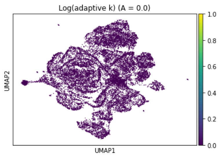
Figure 8: AKNN neighborhood sizes on notMNIST, in increasing order of A𝐴A, plotted on a log scale. Top left figure (A=0𝐴0A=0) represents a 111-NN classifier. Bottom right figure (A=15𝐴15A=15) shows that many of the points’ neighborhoods are maximally large, which can be compared to the right panel of Fig. 7.
Refer to caption
Refer to caption
Figure 9: As Fig. 8, on single-cell mouse data, with the AKNN k-values replaced by their quantiles over the data. The relative ordering of the data by AKNN neighborhood size is fairly robust to A𝐴A. Zoom in or see http://35.239.251.24/aknn/ for details.