Spatial Evolutionary Generative Adversarial Networks

Abstract.

Generative adversary networks (GANs) suffer from training pathologies such as instability and mode collapse. These pathologies mainly arise from a lack of diversity in their adversarial interactions. Evolutionary generative adversarial networks apply the principles of evolutionary computation to mitigate these problems. We hybridize two of these approaches that promote training diversity. One, E-GAN, at each batch, injects mutation diversity by training the (replicated) generator with three independent objective functions then selecting the resulting best performing generator for the next batch. The other, Lipizzaner, injects population diversity by training a two-dimensional grid of GANs with a distributed evolutionary algorithm that includes neighbor exchanges of additional training adversaries, performance based selection and population-based hyper-parameter tuning. We propose to combine mutation and population approaches to diversity improvement. We contribute a superior evolutionary GANs training method, Mustangs, that eliminates the single loss function used across Lipizzaner ’s grid. Instead, each training round, a loss function is selected with equal probability, from among the three E-GAN uses. Experimental analyses on standard benchmarks, MNIST and CelebA, demonstrate that Mustangs provides a statistically faster training method resulting in more accurate networks.

1. Introduction

Generative adversarial networks (GANs) have emerged as a powerful machine learning paradigm. They were first introduced for the task of estimating a distribution function underlying a given set of samples (Goodfellow et al., 2014). A GAN consists of two neural networks, one a generator and the other a discriminator. The discriminator is trained to correctly discern the “natural/real” samples from “artificial/fake” samples produced by the generator. The generator, given a latent random space, is trained to transform its inputs into samples that fool the discriminator. Formulated as a minmax optimization problem through the definitions of discriminator and generator loss, training can converge on an optimal generator, one that approximates the latent true distribution so well that the discriminator can only provide a label at random for any sample.

The early successes of GANs in generating realistic, complex, multivariate distributions motivated a growing body of applications, such as image generation (Gan et al., 2017), video prediction (Liang et al., 2017), image in-painting (Yeh et al., 2017), and text to image synthesis (Reed et al., 2016). However, while the competitive juxtaposition of the generator and discriminator is a compelling design, GANs are notoriously hard to train. Frequently training dynamics show pathologies. Since the generator and the discriminator are differentiable networks, optimizing the minmax GAN objective is generally performed by (variants of) simultaneous gradient-based updates to their parameters (Goodfellow et al., 2014). This type of gradient-based training rarely converges to an equilibrium. GAN training thus exhibits degenerate behaviors, such as mode collapse (Arora et al., 2018), discriminator collapse (Li et al., 2017b), and vanishing gradients (Arjovsky and Bottou, 2017).

Different objectives impact the gradient information used to update parameters weights of the networks. Therefore, changing the objective impacts the search trajectory and could eliminate or decrease the frequency of pathological trajectories. A set of recent studies by members of the machine learning community proposed different objective functions. Generally, these functions compute loss as the distance between the fake data and real data distributions according to different measures. The original GAN (Goodfellow et al., 2014) applies the Jensen-Shannon divergence (JSD). Other measures include: 1) Kullback-Leibler divergence (KLD)(Nguyen et al., 2017), 2) the Wasserstein distance (Arjovsky et al., 2017), 3) the least-squares (LS) (Mao et al., 2017), and 4) the absolute deviation (Zhao et al., 2016).

Each of these objective functions improves training but none entirely solves all of its challenges. An evolutionary computation project investigated an evolutionary generative adversarial network (E-GAN), a different approach (Wang et al., 2018). E-GAN, batch after batch, is able to guide its trajectory with gradient information from a population of three different objectives, which defines the gradient-based mutation to be applied. As we will describe in more detail in Section 2, each batch, E-GAN trains each of three copies of the GAN with one of the three objectives in the population. After this independent training, E-GAN selects the best GAN according to a given fitness function to start the next batch and train further. This process splices batch-length trajectories from different gradient information together. Essentially, E-GAN injects mutation diversity into training. As a result, on some benchmarks, E-GAN improves and provides comparable performance on a baseline using a single objective.

Another evolutionary computation idea for addressing training pathologies comes from competitive coevolutionary algorithms. With one population adversarially posed against another, they optimize with a minmax objective like GANs. Pathologies similar to what is reported in GAN training have been observed in coevolutionary algorithms, such as focusing, relativism, and lost of gradient (Popovici et al., 2012). They have been attributed to a lack of diversity. Each population converges or the coupled population dynamics lock into a tit-for-tat pattern of ineffective signaling. Spatial distributed populations have been demonstrated to be particularly effective at resolving this. This approach has been transferred to GANs with Lipizzaner (Schmiedlechner et al., 2018; Al-Dujaili et al., 2018). Lipizzaner uses a spatial distributed competitive coevolutionary algorithm. It places the individuals of the generator and discriminator populations on a grid (each cell contains a pair of generator-discriminators). Each generator is evaluated against all the discriminators of its neighborhood and the same happen with each discriminator. Lipizzaner takes advantage of neighborhood communication to propagate models. Lipizzaner, in effect, provides diversity in the genome space.

In this paper we ask whether a method that capitalizes on ideas from both E-GAN and Lipizzaner is better than either one of them. Specifically, can a combination of diversity in mutation and genome space train GANs faster, more accurately and more reliably? Thus, we present the MUtation SpaTial gANs training method, Mustangs. For each cell of the grid, Mustangs selects randomly with equal probability a given loss function from among the set of three that E-GAN introduced, which is applied for the current training batch. This process is repeated for each batch during the whole GAN training. We experimentally evaluate Mustangs on standard benchmarks, MNIST and CelebA, to determine whether it provides more accurate results and/or requires shorter execution times. The main contributions of this paper are: 1) Mustangs, a training method of GANs that provides both mutation and genome diversity. 2) A open source software implementation of Mustangs , 3) A demonstration of Mustangs’s higher accuracy and performance on MNIST and CelebA. 4) A deployment of Mustangs on cloud computing infrastructure that optimizes the GAN grid in parallel.

The rest of the paper is organized as follows. Section 2 presents related work. Section 3 describes the method. The experimental setup and the results are in sections 4 and 5. Finally, conclusions are drawn and future work is outlined in Section 6.

2. Related work

Recent work have focused on improving the robustness of GAN training and the overall quality of generated samples (Arjovsky and Bottou, 2017; Arora et al., 2018; Nguyen et al., 2017). Prior approaches tried to mitigate degenerate GAN dynamics by using heuristics, such as decreasing the optimizer’s learning rate along the iterations (Radford et al., 2015). Other authors have proposed changing generator’s or discriminator’s objectives (Arjovsky et al., 2017; Mao et al., 2017; Nguyen et al., 2017; Zhao et al., 2016). More advanced methods apply ensemble approaches (Wang et al., 2016).

A different category of studies employ multiple generators and/or discriminators. Some remarkable examples analyze training a cascade of GANs (Wang et al., 2016); sequentially training and adding new generators with boosting techniques (Tolstikhin et al., 2017); training in parallel multiple generators and discriminators (Jiwoong Im et al., 2016); and training an array of discriminators specialized in a different low-dimensional projection of the data (Neyshabur et al., 2017).

Recent work by Yao and co-authors proposed E-GAN, whose main idea is to evolve a population of three independent loss functions defined according to three distance metrics (JSD, LS, and a metric based on JSD and KL) (Wang et al., 2018). One at a time, independently, the loss functions are used to train a generator from some starting condition, over a batch. The generators produced by the loss functions are evaluated by a single discriminator (considered optimal) that returns a fitness value for each generator. The best generator of the three options is then selected and training continues, with the next training batch, and the three different loss functions. The use of different objective functions (mutations) overcomes the limitations of a single individual training objective and a better adapts the population to the evolution of the discriminator. E-GAN defines a specific fitness function that evaluates the generators in terms of the quality and the diversity of the generated samples. The results shown that E-GAN is able to get higher inception scores, while showing comparable stability when it goes to convergence. E-GAN works because the evolutionary population injects diversity into the training. Over one training run, different loss functions inform the best generator of a batch.

Another evolutionary way to improve training is also motivated by diversity (Schmiedlechner et al., 2018; Al-Dujaili et al., 2018). Lipizzaner simultaneously trains a spatially distributed population of GANs (pairs of generators and discriminators) that allows neighbors to communicate and share information. Gradient learning is used for GAN training and evolutionary selection and variation is used for hyperparameter learning. Overlapping neighborhoods and local communication allow efficient propagation of improving models. Besides, this strategy has the ability to distribute the training process on parallel computation architectures, and therefore, it can efficiently scale. Lipizzaner coevolutionary dynamics are able to escape degenerate GAN training behaviors, e.g, mode collapse and vanishing gradient, and resulting generators provide accurate and diverse samples.

In this paper we ask whether an advance that capitalizes on ideas from both E-GAN (i.e., diversity in the mutation space) and Lipizzaner (i.e., diversity in genomes space) is better than either one of them.

Figure 1. Spatial coevolution training on a $3\times 3$ grid (Al-Dujaili et al., 2018). $P_{v}=\{v_{1},\dots v_{9}\}$ and $P_{u}=\{u_{1},\dots u_{9}\}$ denote neural network weights of discriminator and generator population respectively. $P_{\gamma}=\{\gamma_{1},\dots,\gamma_{9}\}$ and $P_{\delta}=\{\delta_{1},\dots,\delta_{9}\}$ denote the hyperparameters (e.g., learning rate) of discriminator and generator population, respectively. $P_{\bf w}=\{\mathbf{w}_{1},\dots,\mathbf{w}_{9}\}$ denote the mixture weights. The $(\cdot)^{\prime}$ notation denotes the value of $(\cdot)$ after one iteration of coevolution.

3. Mustangs Method

This section presents Mustangs devised in this work. First, we introduce the general optimization problem of GAN training. Then, we describe a method for spatial coevolution GANs training. Finally, we present the multiple mutations applied to produce the generators offspring.

3.1. General GAN Training

In this paper we adopt a mix of notation used in (Li et al., 2017b). Let $\mathcal{G}=\{G_{u},u\in\mathcal{U}\}$ and $\mathcal{D}=\{D_{v},v\in\mathcal{V}\}$ denote the class of generators and discriminators, respectively, where $G_{u}$ and $D_{v}$ are functions parameterized by $u$ and $v$. $\mathcal{U},\mathcal{V}\subseteq\operatorname{\mathbb{R}}^{p}$ represent the parameters space of the generators and discriminators, respectively. Further, let $G_{*}$ be the target unknown distribution that we would like to fit our generative model to.

Formally, the goal of GAN training is to find parameters $u$ and $v$ so as to optimize the objective function

$$\min_{hu\in\mathcal{U}}\max_{v\in\mathcal{V}}\mathcal{L}(u,v)\;,\;\text{where}$$

(1) $$\mathcal{L}(u,v)=\operatorname{\mathbb{E}}_{x\sim G_{*}}[\phi(D_{v}(x))]+\operatorname{\mathbb{E}}_{x\sim G_{u}}[\phi(1-D_{v}(x))]\;,$$

and $\phi:[0,1]\to\operatorname{\mathbb{R}}$, is a concave function, commonly referred to as the measuring function. In practice, we have access to a finite number of training samples $x_{1},\ldots,x_{m}\sim G_{*}$. Therefore, an empirical version $\frac{1}{m}\sum_{i=1}^{m}\phi(D_{v}(x_{i}))$ is used to estimate $\operatorname{\mathbb{E}}_{x\sim G_{*}}[\phi(D_{v}(x))]$. The same holds for $G_{u}$.

3.2. Spatial Coevolution for GAN Training

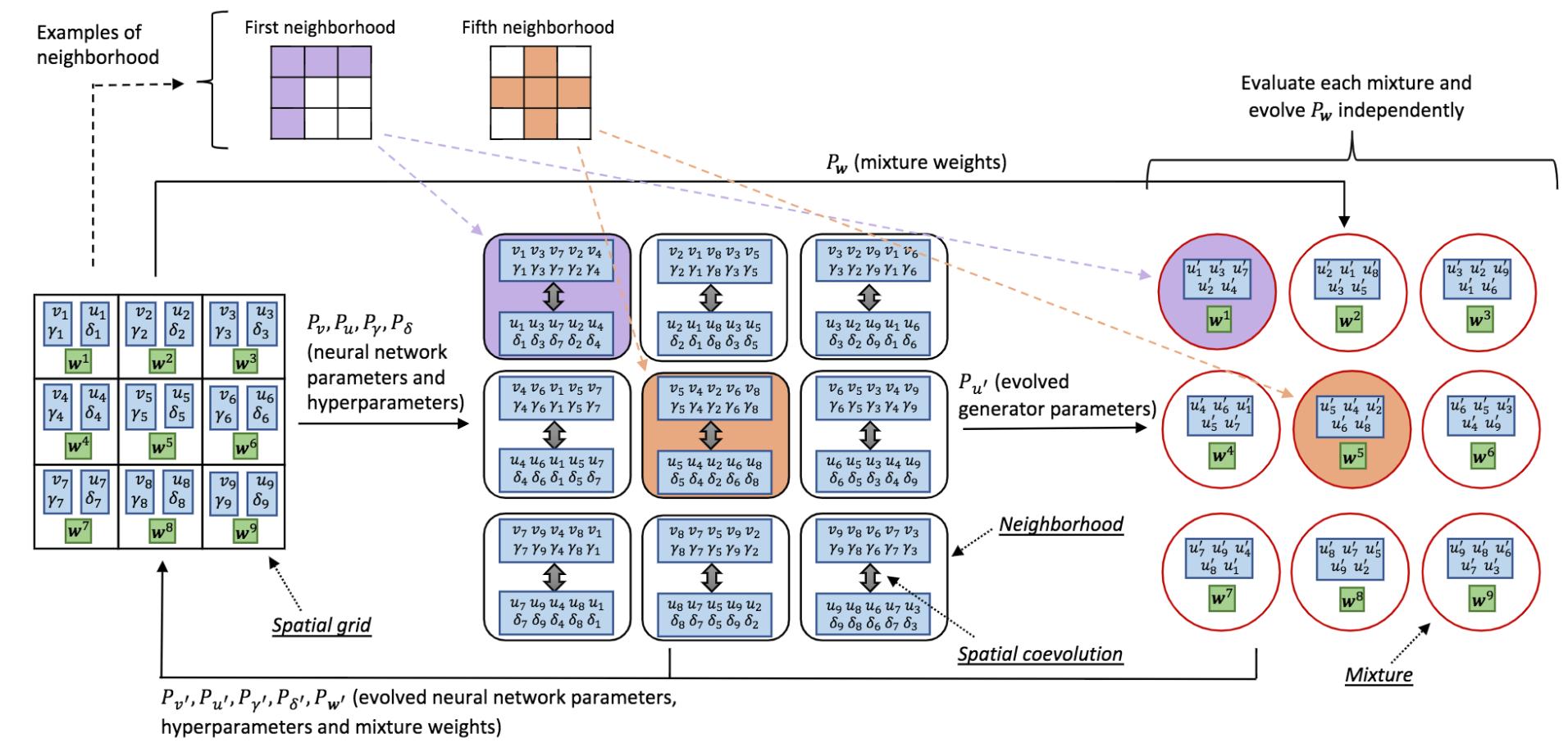
Evolutionary computation implements mechanisms inspired by biological evolution such as reproduction, diversity generation, and survival of the fittest to address optimization problems. In this case. we apply the competitive coevolutionary algorithm outlined in Algorithm 1 to optimize GANs. It evolves two populations, $P_{u}=\{u_{1},\ldots,u_{T}\}$ a population of generators and $P_{v}=\{v_{1},\ldots,v_{T}\}$ a population of discriminators to create diversity in genomes spaces, where $T$ is the population size. The fitness $\mathcal{L}$ of each generator $u_{i}\in P_{u}$ and discriminator $v_{j}\in P_{v}$ are assessed according to their interactions with a set of discriminators from $P_{v}$ and generators from $P_{u}$, respectively (Lines 3 to 8). The fittest individuals are used to generate the new of individuals (generators and discriminators) by applying mutation (see Section 3.3). The new individuals replace the ones in the current population if they perform better (better fitness) to produce the next generation.

Mustangs applies the spatially distributed coevolution summarized in Algorithm 1, the individuals of both populations (generators of $P_{u}$ and discriminators of $P_{v}$) are distributed on the cells of a two imensional toroidal grid (Al-Dujaili et al., 2018). Spatial coevolution has shown a considerable ability in maintaining diversity in the populations and fostering continuous arms races (Mitchell et al., 2006; Williams and Mitchell, 2005).

Algorithm 1 GeneralCoevGANs($P_{u},P_{v},\mathcal{L},\{\alpha_{i}\},\{\beta_{i}\},p_{\mu},$)
Input:
 $P_{u}$ : generator population                                    $P_{v}$ : discriminator population
 $\{\alpha_{i}\}$ : selection probability                                $\{\beta_{i}\}$ : mutation probability
 $I$ : number of generations                                    $\mathcal{L}$ : GAN objective function
 $p_{\mu}$ : objective-selection probabilities vector
Return:
 $P_{u}$ : evolved generator population
 $P_{v}$ : evolved discriminator population

1:for $i$ in $[1\ldots I]$ do

2:     // Evaluate $P_{u}$ and $P_{v}$

3:    $f_{u_{1}\ldots u_{T}}\leftarrow 0$

4:    $f_{v_{1}\ldots v_{T}}\leftarrow 0$

5:    for each $u_{i}$ in $P_{u}$, each $v_{j}$ in $P_{v}$ do

6:        $f_{u_{i}}\mathrel{-}=\mathcal{L}(u_{i},v_{j})$

7:        $f_{v_{j}}\mathrel{+}=\mathcal{L}(u_{i},v_{j})$

8:    end for

9:     // Sort $P_{u}$ and $P_{v}$

10:    $u_{1\ldots T}\leftarrow u_{s(1)\ldots s(T)}\texttt{ with }s(i)=\texttt{argsort}(f_{u_{1}\ldots u_{T}},i)$

11:    $v_{1\ldots T}\leftarrow v_{s(1)\ldots s(T)}\texttt{ with }s(j)=\texttt{argsort}(f_{v_{1}\ldots v_{T}},j)$

12:     // Selection

13:    $u_{1\ldots T}\leftarrow u_{s(1)\ldots s(T)}\texttt{ with }s(i)=\texttt{argselect}(u_{1\ldots T},i,\{\alpha_{i}\})$

14:    $v_{1\ldots T}\leftarrow v_{s(1)\ldots s(T)}\texttt{ with }s(j)=\texttt{argselect}(v_{1\ldots T},j,\{\alpha_{j}\})$

15:     // Mutation & Replacement

16:    $u_{1\ldots T}\leftarrow\texttt{replace}(\{u_{i}\},\{u^{\prime}_{i}\})\texttt{ with }u^{\prime}_{i}=\texttt{mutateP${}_{u}$}(u_{i},\{\beta_{i}\})$

17:    $v_{1\ldots T}\leftarrow\texttt{replace}(\{v_{j}\},\{v^{\prime}_{j}\})\texttt{ with }v^{\prime}_{j}=\texttt{mutateP${}_{v}$}(v_{j},\{\beta_{i}\})$

18:end for

19:return $P_{u},P_{v}$

The cell’s neighborhood defines the subset of individuals of $P_{u}$ and $P_{v}$ to interact with and it is specified by its size $s_{n}$. Given a $m\times n$-grid, there are $m\times n$ neighborhoods. Without losing generality, we consider $m^{2}$ square grids to simplify the notation. In our study, we use a five-cell neighborhood, i.e, one center and four adjacent cells (see Figure  1). We apply the same notation used in (Al-Dujaili et al., 2018). For the $k$-th neighborhood in the grid, we refer to the generator in its center cell by $P^{k,1}_{u}\subset P_{u}$ and the set of generators in the rest of the neighborhood cells by $P^{k,2}_{u},\ldots,P^{k,s_{n}}$, respectively. Furthermore, we denote the union of these sets by $P^{k}_{u}=\cup^{s_{n}}_{i=1}P^{k,i}_{u}\subseteq P_{u}$, which represents the $k$th generator neighborhood.

In the spatial coevolution applied here, each neighborhood performs an instance of Algorithm 1 with the populations $P^{k}_{u}$ and $P^{k}_{v}$ to update its center cell, i.e. $P^{k,1}_{u}$, $P^{k,1}_{v}$, with the returned values (Line 19 of Algorithm 1).

Given the $m^{2}$ neighborhoods, all the individuals of $P_{u}$ and $P_{v}$ will get updates as $P_{u}=\cup^{m^{2}}_{k=1}P^{k}_{u}$, $P_{v}=\cup^{m^{2}}_{k=1}P^{k}_{v}$. These $m^{2}$ instances of Algorithm 1 run in parallel in an asynchronous fashion when dealing with reading/writing from/to the populations. This implementation scales with lower communication overhead, allows the cells to run its instances without waiting each other, increases the diversity by mixing individuals computed during different stages of the training process, and performs better with limited number of function evaluations (Nielsen et al., 2012).

Taking advantage of the population of $|P_{u}|$ generators trained, the spatial coevolution method selects one of the generator neighborhoods $\{P^{k}_{u}\}_{1\leq k\leq m^{2}}$ as a mixture of generators according to a given performance metric $f:\mathcal{U}^{s_{n}}\times\operatorname{\mathbb{R}}^{s_{n}}\to\operatorname{\mathbb{R}}$. Thus, it is chosen the best generator mixture $P^{*}_{u}\in\mathcal{U}^{s_{n}}$ according to the mixture weights $\bm{w}^{*}\in[0,1]^{s_{n}}$. Hence, the $s_{n}$-dimensional mixture weight vector $\bm{w}$ is defined as follows

(2) $$\footnotesize P^{*}_{u},\bm{w}^{*}=\operatorname*{arg\,max}_{P^{k}_{u},\bm{w}^{k}:1\leq k\leq m^{2}}f\big{(}\sum_{{u_{i}\in P^{k}_{u}\\ w_{i}\in\bm{w}^{k}}}w_{i}G_{u_{i}}\big{)}\;,$$

where $w_{i}$ represents the mixture weight of (or the probability that a data point comes from) the $i$th generator in the neighborhood, with $\sum_{w_{i}\in\bm{w}^{k}}w_{i}=1$. These hyperparameters $\{\bm{w}^{k}\}_{1\leq k\leq m^{2}}$ are optimized during the training process after each step of spatial coevolution by applying an evolution strategy (1+1)-ES (Al-Dujaili et al., 2018).

3.3. Mustangs Gradient-based Mutation

Mustangs coevolutionary algorithm generates the offspring of both populations $P_{h}$ and $P_{q}$ by by applying asexual reproduction, i.e. next generation’s of individuals are produced by applying mutation (Lines 16 and 17 in Algorithm 1). These mutation operators are defined according to a giving training objective, which generally attempts to minimize the distance between the generated fake data and real data distributions according to a given measure. Lipizzaner applies the same gradient-based mutation for both populations during the coevolutionary learning (Al-Dujaili et al., 2018).

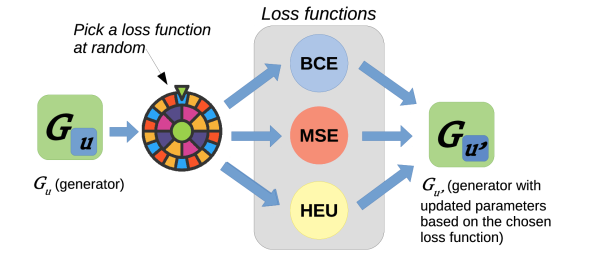
In this study, we add mutation diversity to the genome diversity provided by Lipizzaner. Thus, we use the mutations used by E-GAN to generate the offspring of generators (Wang et al., 2018). E-GAN applies three different mutations corresponding with three different minimization objectives w.r.t. the generator: 1) Minmax mutation, which objective is to minimize the JSD between the real and fake data distributions, i.e., $JSD(p_{real}\parallel p_{fake})$ (see Equation (3)). 2) Least-square mutation, which is inspired in the least-square GAN (Mao et al., 2017) that applies this criterion to adapt both, the generator and the discriminator. The objective function is formulated as shown in Equation (4). 3) Heuristc mutation, which maximizes the probability of the discriminator being mistaken by minimizing the objective function in Equation (5). This objective is equal to minimizing $[KL(p_{real}\parallel p_{fake})-2JSD(p_{real}\parallel p_{fake})]$

(3) $$M^{minmax}_{G}=\frac{1}{2}\operatorname{\mathbb{E}}_{x\sim G_{u}}[log(1-D_{v}(x))]$$

(4) $$M^{least-square}_{G}=\operatorname{\mathbb{E}}_{x\sim G_{u}}[log(D_{v}(x)-1)^{2}]$$

(5) $$M^{heuristic}_{G}=\frac{1}{2}\operatorname{\mathbb{E}}_{x\sim G_{u}}[log(D_{v}(x))]$$

Thus, the mutation applied to the generators (mutateP_u) in Line 16 of Algorithm 1 is defined in the Algorinthm 2. The new generator is produced by using a loss function (mutation) to optimize one of the three objectives functions introduced above. i.e., $M^{minmax}_{G}$, $M^{least-square}_{G}$, and $M^{heuristic}_{G}$, which are binary cross entropy (BCE) loss, mean square error (MSE) loss, and heuristic loss, respectively.

E-GAN applies the three mutations to the generator (ancestor) and it selects the individual that provides the best fitness when is evaluated against the discriminator (Wang et al., 2018). In contrast, Mustangs picks at random with same the probability ($\frac{1}{3}$) one of the mutations (loss functions), as it is shown in Figure 2, and then the gradient descent method is applied accordingly (see Algorithm 2). This enables diversity in the mutation space without adding noticeable overhead over the spatial coevolutionary training method presented before, since Mustangs evaluates only the mutated generator instead of three as E-GAN does.

Figure 2. Graphical representation of the mutation used in Mustangs. The generator (ancestor) $G_{u}$ is mutated to produce the new generator $G_{u\prime}$ by using one of the loss functions chosen at random.

Algorithm 2 mutateP_u($u$)
Input:
 $u$ : generator parameters
Return:
 $u^{\prime}$ : mutated generator parameters

1:$operator\leftarrow\texttt{pick\_random}[1\ldots 3]$

2:if $operator==1$ then

3:    $u^{\prime}\leftarrow\texttt{applyGradienDescent}(M^{minmax}_{G},u)$

4:else if $operator==2$ then

5:    $u^{\prime}\leftarrow\texttt{applyGradienDescent}(M^{least-square}_{G},u)$

6:else

7:    $u^{\prime}\leftarrow\texttt{applyGradienDescent}(M^{heuristic}_{G},u)$

8:end if

9:return $u^{\prime}$

E-GAN, Lipizzaner, and Mustangs apply the same mutation (loss function) to update the discriminators, the one defined to address the GAN minmax optimization problem described in Equation (3.1).

4. Experimental Setup

Mustangs is evaluated on two common image data sets: MNIST and CelebA. The experiments compare the following methods:

1. a standard GAN which uses $M^{minmax}_{G}$ objective

2. the E-GAN method

3. Lipizzaner with $M^{minmax}_{G}$ objective

4. Lipizzaner with $M^{least-square}_{G}$ objective

5. Lipizzaner with $M^{heuristic}_{G}$ objective

6. the Mustangs method

The settings used for the experiments are summarized in Table 1. The four spatial coveolutionary GANs use the parameters presented in Table 1. E-GAN and GAN-BCE both use the Adam optimizer with an initial learning rate (0.0002). The other parameters of E-GAN use the same configuration as used in (Wang et al., 2018).

For MNIST data set experiments, all methods use the same stop condition: a computational budget of nine hours (9h). The distributed methods of Mustangs, Lip-BCE, Lip-MSE, and Lip-HEU use a grid size of $3\times 3$, and are able to train nine networks in parallel. Thus, they are executed during one hour to comply with the computational budget of nine hours. Regarding CelebA experiments, the four spatial coveolutionary GANs are analyzed. Thus, they stop after performing 20 training epochs, since they require similar computational budget to perform them.

All methods have been implemented in Python3 and pytorch. The spatial coevolutionary ones have extended the Lipizzaner framework (Schmiedlechner et al., 2018).

The experimental analysis is performed on a cloud computation platform that provides 8 Intel Xeon cores 2.2GHz with 32 GB RAM and a NVIDIA Tesla T4 GPU with 16 GB RAM. We run multiple independent runs for each method.

Table 1. Network topology of the GANs trained.

Parameter	MNIST	CelebA
Network topology
Network type	MLP	DCGAN
Input neurons	64	100
Number of hidden layers	2	4
Neurons per hidden layer	256	16,384 - 131,072
Output neurons	784	64$\times$64$\times$64
Activation function	$tanh$	$tanh$
Training settings
Batch size	100	128
Skip N disc. steps	1	-
Coevolutionary settings
Stop condition	9 hours comp.	20 training epochs
Population size per cell	1	1
Tournament size	2	2
Grid size	3$\times$3	2$\times$2
Performance metric ($m$)	FID	FID
Mixture mutation scale	0.01	0.01
Hyperparameter mutation
Optimizer	Adam	Adam
Initial learning rate	0.0002	0.00005
Mutation rate	0.0001	0.0001
Mutation probability	0.5	0.5

For quantitative assessment of the accuracy of the generated fake data the Frechet inception distance (FID) is evaluated (Heusel et al., 2017). We analyze the computational performance of each method. Finally, we evaluate the diversity of the data samples generated.

5. Results and Discussion

This section presents the results and the analyses of the studied optimization methods. The first three subsections evaluate the MNIST experiments in terms of the FID score, the computational performance, and the diversity of the generated samples, respectively. The last one analyzes the CelebA results in terms of FID score.

5.1. Quality of the Generated Data

Table 2 shows the best FID value from each of the 30 independent runs performed for each method. Mustangs has the lowest median (see Figure 3 for a boxplot). All the methods that used Lipizzaner are better than E-GAN and GAN-BCE. However, there is quite a significant increase in FID value between the Lip-MSE and the other Lipizzaner based methods. The results indicate that Mustangs is robust to the varying performance of the individual loss functions and can still find a high performing mixture of generators. This helps to strengthen the idea that diversity, both in genome and mutation space, provides robust GAN training.

Table 2. FID MNIST results in terms of best mean, normalized standard deviation, median and interquartile range (IQR). (Low FID indicates good performance)

Algorithm	Mean	Std%	Median	IQR
Mustangs	42.235	12.863%	43.181	7.586
Lip-BCE	48.958	20.080%	46.068	4.663
Lip-MSE	371.603	20.108%	381.768	104.625
Lip-HEU	52.525	17.230%	52.732	9.767
E-GAN	466.111	10.312%	481.610	69.329
GAN-BCE	457.723	2.648%	459.629	17.865

The results provided by the methods that generates diversity in genome space only (Lip-BCE, Lip-HEU, and Lip-MSE) are significantly more competitive than E-GAN, which provides diversity in mutation space only (see Figure 3). Therefore, the spatial distributed coevolution provides an efficient tool to optimize GANs.

Figure 3. Results on MNIST dataset. Boxplot that shows the best FIDs computed for each independent run.

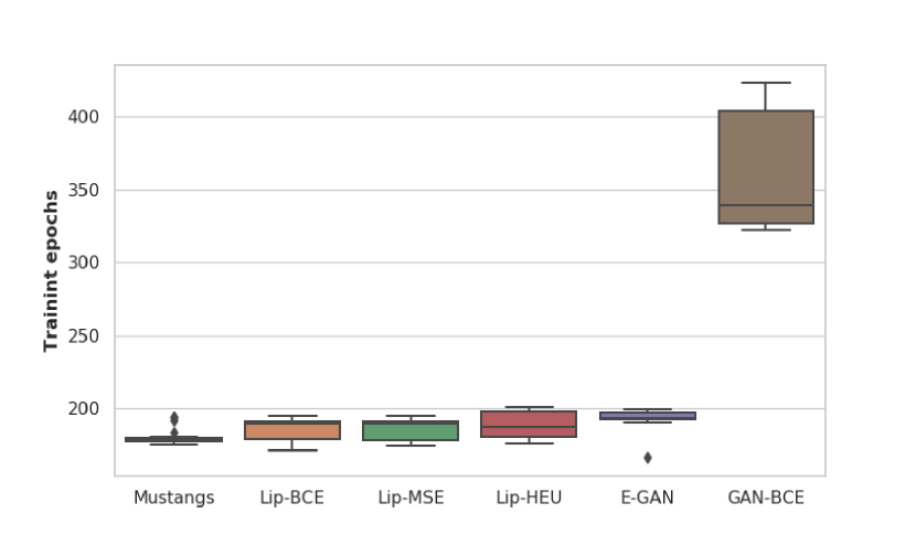
Surprisingly the median FID score of GAN-BCE is better than E-GAN. E-GAN has a larger variance of FID scores compared to GAN-BCE, and in the original paper it was shown that E-GAN performance improved with more epochs (by using a computational budget of 30h, compared to the 9h we use here).

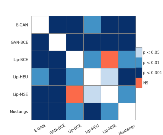
The results in Table 2 indicate that spatialy distributed coevolutionary training is the best choice to train GANs, even when there is no knowledge about the best loss function to the problem. However, the choice of loss function (mutation) may impact the final results. In summary, the combination of both mutation and genome diversity significantly provides the most best result. A ranksum test with Holm correction confirms that the difference between Mustangs and the other methods is significant at confidence levels of $\alpha$=0.01 and $\alpha$=0.001 (see Figure 4).

Figure 4. Holm statistical post-hoc analysis on MNIST dataset. It illustrates the $p$-values computed by the statistical tests.

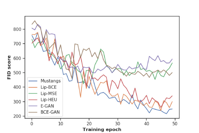
Next, we evaluate the FID score through out the GAN training process, see Figure 5 illustrates the FID changes during the entire training process. In addition, we zoom in on the first 50 training epochs in Figure 6. None of the evolutionary GAN training methods seem to have converged after 9h of computation. This implies that longer runs can further improve the results.

According to Figure 5, the robustness of the three most competitive methods (Mustangs, Lip-BCE, and Lip-HEU) indicates that the FID almost behaves like a monotonically decreasing function with small oscilations. The other three methods have larger osilations and does not seem to have a FID trend that decreases with the same rate.

Focusing on the two methods that apply the same unique loss function in Equation (3), GAN-BCE and Lip-BCE, we can clearly state the benefits of the distributed spatial evolution. Even the two methods provide comparable FID during the first 30 training epochs, Lip-BCE converges faster to better FID values (see Figure 6). This difference is even more noticeable when both algorithms consume the 9h of computational cost (see Figure 5).

Figure 5. Results on MNIST dataset. FID evolution through the training process during 9h of computational cost.

Figure 6. Results on MNIST dataset. FID evolution through the first 50 epochs of the training process.

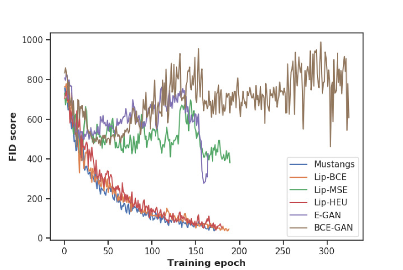
Notice that the spatial coevolutionary methods use FID as the objective function to select the best mixture of generators during the optimization of the GANs. In contrast, E-GAN applies a specific objective function based on the losses (Wang et al., 2018) and GAN-BCE optimizes just one network.

5.2. Computational Performance

In this section, we analyze the computational performance of the GAN training methods, all used the same computational budget (9h). We start analyzing the number of training epochs. As Mustangs and Lipizzaner variations apply asynchronous parallelism, the number of training epochs performed by each cell of the grid in the same run varies. Thus, for these methods, we consider that the number of training epochs of a given run is the mean of the epochs performed by each cell.

Table 3 shows the mean, normalized standard deviation, minimum, and maximum values of number of training epochs. The number of epochs are normally distributed for all the algorithms. Please note that, first, all the analyzed methods have been executed on a cloud architecture, which could generate some differences in terms of computational efficiency results; and second, everything is implemented by using the same Python libraries and versions to limit computational differences between them due to the technologies used.

Table 3. Results on MNIST dataset. Mean, normalized standard deviation, minimum, median and maximum of training epochs.

Algorithm	Mean	Std%	Minimum	Median	Maximum
Mustangs	179.456	2.708%	174.778	177.944	194.000
Lip-BCE	185.919	4.072%	171.222	189.444	194.333
Lip-MSE	185.963	3.768%	173.667	189.222	194.778
Lip-HEU	188.644	4.657%	175.667	186.667	200.556
E-GAN	193.167	2.992%	166.000	193.000	199.000
GAN-BCE	365.267	10.570%	322.000	339.500	423.000

Figure 7. Results on MNIST dataset. Boxplot of the number of training epochs.

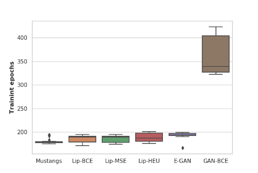
The method that is able to train each network for the most epochs is GAN-BCE. However, this method trains only one network, in contrast to the other evaluated methods. GAN-BCE performs about two times the number of iterations of E-GAN, which evaluates three networks.

The spatially distributed coevolutionary algorithms performed significantly fewer training epochs than E-GAN. However, during each epoch these methods evaluate 45 GANs, i.e., neighborhood size of 5 $\times$ 9 cells, which is 15 times more networks than E-GAN.

One of the most important features of the spatial coevolutionary algorithm is that it is executed asynchronously and in parallel for all the cells (Schmiedlechner et al., 2018). Thus, there is no bottleneck for each cells performance since it operates without waiting for the others. In future work E-GAN could take advantage of parallelism and optimizing the three discriminators at the same time. However, it has an important synchronization bottleneck because they are evaluated over the same discriminator, which is trained and evaluated sequentially after that operation.

5.3. Diversity of the Generated Outputs

In this section, we evaluate the diversity of the generated samples by the networks that had the best FID score. We report the the total variation distance (TVD) for each algorithm (Li et al., 2017a) (see Table 4).

Table 4. Results on MNIST dataset. TVD results. (Low TVD indicates more diversity)

Alg.	Mustangs	Lip-BCE	Lip-HEU	Lip-MSE	E-GAN	GAN-BCE
TVD	0.180	0.171	0.115	0.365	0.534	0.516

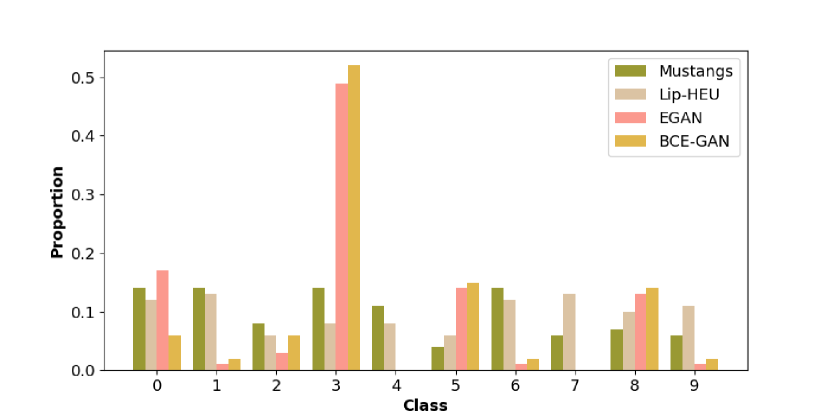
The methods that provide genome diversity generate more diverse data samples than the other two analyzed methods. This shows that genomic diversity introduces a capability to avoid mode collapse situations as the one shown in Figure 9(a). The three algorithms with the lowest FID score (Mustangs, Lip-BCE, and Lip-HEU) also provide the lowest TVD values. The best TVD result is obtained by Lip-HEU.

The distribution of each class of digits for generated images is shown in Figure 8. The diagram supports the TVD results, e.g. Lip-HEU and Mustangs produce more diverse set of samples spanning across different classes. We can observe that the two methods that do not apply diversity in terms of genome display a possible mode collapse, since about half of the samples are of class 3 and they not generate samples of class 4 and 7.

Figure 8. Classes distribution of the samples generated of MNIST by Mustangs, Lip-HEU, E-GAN, and GAN-BCE.

(a) Mode collapse	(b) Mustangs	(c) Lip-BCE	(d) Lip-HEU	(e) Lip-MSE	(f) E-GAN	(g) GAN-BCE

Figure 9. Sequence of samples generated of MNIST dataset. (a) contains for mode collapse, the generator is focused on the character 0. It illustrates samples generated by the best generator (in terms of FID) by Mustangs (b), Lip-BCE (c), Lip-HEU (d), Lip-MSE (e), E-GAN (f), and GAN-BCE (g).

Figure 9 illustrates how spatially distributed coevolutionary algorithms are able to produce robust generators that provide with accurate samples across all the classes.

5.4. CelebA Experimental Results

The spatially distributed coevolutionary methods are applied to perform the CelebA experiments. Table 5 summarizes the results over multiple independent runs.

Table 5. Results on CelebA dataset. FID results in terms of best mean, normalized standard deviation, median and interquartile range (IQR). (Low FID indicates good performance)

Algorithm	Mean	Std%	Median	IQR
Mustangs	36.148	0.571%	36.087	0.237
Lip-BCE	36.250	5.676%	36.385	2.858
Lip-MSE	158.740	40.226%	160.642	47.216
Lip-HEU	37.872	5.751%	37.681	2.455

Mustangs provides the lowest median FID and Lip-MSE the highest one. Lip-BCE and Lip-HEU provide median and average FID scores close to the Mustangs ones. However, Mustangs is more robust to the varying performance of the methods that apply a unique loss function (see deviations in Table 5).

The robustness of the training provided by Mustangs makes it an efficient tool when the computation budget is limited (i.e., performing a limited number of independent runs), since it shows low variability in its competitive results.

Next, we evaluate the FID score through the training process. Figure 10 shows the FID changes during the entire training process. All the analyzed methods behave like a monotonically decreasing function. However, the FID evolution of Lip-BCE presents oscillations. Mustangs, Lip-BCE, and Lip-HEU FIDs show a similar evolution.

Figure 10. Results on CelebA dataset. FID evolution through the 20 epochs of the training process.

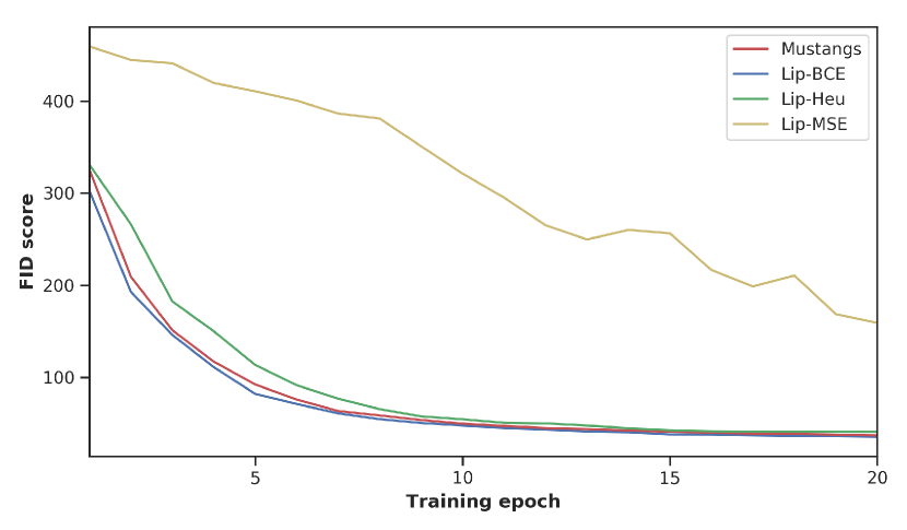
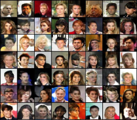
Figure 11 illustrates a sequence of samples generated by the best mixture of generators in terms of FID score of the most competitive two training methods, i.e., Mustangs and Lip-BCE. As it can be seen in these two sets images generated, both methods present similar capacity of generating human faces.

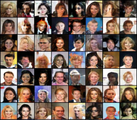(a) Mustangs	(b) Lip-BCE

Figure 11. Sequence of samples generated of CelebA. It illustrates samples generated by the best mixture of generators (in terms of FID) by Mustangs (a) and Lip-BCE (b).

6. Conclusions and Future Work

We have empirically showed that GAN training can be improved by boosting diversity. We enhanced an existing spatial evolutionary GAN training framework that promoted genomic diversity by probabilistically choosing one of three loss functions. This new method, called Mustangs was tested on the MNIST and CelebA data sets showed the best performance and high diversity in label space, as well as on the TVD measure. The high performance of Mustangs is due to its inherent robustness. This allows it to overcome often observed training pathologies, e.g. mode collapse. Furthermore, the Mustangs method can be executed asynchronously and the computation is easy to distribute with low overhead. We extended the Lipizzaner open source implementation to demonstrate this.

Future work will include the evaluation of Mustangs on more data sets and longer training epochs. We can also include other loss functions. In addition, we are exploring the diversity of the networks over their neighborhoods and the whole grid when applying the different methods studied here. This study will be a first step in devising an algorithm that self-adapts the probabilities of the different mutations dynamically. Finally, other advancements in evolutionary algorithms that can improve the robustness of GAN training, e.g. temporal evolutionary training, need to be considered.

References

- (1)
- Al-Dujaili et al. (2018) Abdullah Al-Dujaili, Tom Schmiedlechner, Erik Hemberg, and Una-May O’Reilly. 2018. Towards distributed coevolutionary GANs. In AAAI 2018 Fall Symposium.
- Arjovsky and Bottou (2017) Martin Arjovsky and Léon Bottou. 2017. Towards principled methods for training generative adversarial networks. arXiv preprint arXiv:1701.04862 (2017).
- Arjovsky et al. (2017) Martin Arjovsky, Soumith Chintala, and Léon Bottou. 2017. Wasserstein GAN. arXiv preprint arXiv:1701.07875 (2017).
- Arora et al. (2018) Sanjeev Arora, Andrej Risteski, and Yi Zhang. 2018. Do GANs learn the distribution? Some Theory and Empirics. In International Conference on Learning Representations. https://openreview.net/forum?id=BJehNfW0-
- Gan et al. (2017) Zhe Gan, Liqun Chen, Weiyao Wang, Yuchen Pu, Yizhe Zhang, Hao Liu, Chunyuan Li, and Lawrence Carin. 2017. Triangle generative adversarial networks. In Advances in Neural Information Processing Systems. 5247–5256.
- Goodfellow et al. (2014) Ian Goodfellow, Jean Pouget-Abadie, Mehdi Mirza, Bing Xu, David Warde-Farley, Sherjil Ozair, Aaron Courville, and Yoshua Bengio. 2014. Generative adversarial nets. In Advances in neural information processing systems. 2672–2680.
- Heusel et al. (2017) Martin Heusel, Hubert Ramsauer, Thomas Unterthiner, Bernhard Nessler, Günter Klambauer, and Sepp Hochreiter. 2017. GANs trained by a two time-scale update rule converge to a nash equilibrium. arXiv preprint arXiv:1706.08500 12, 1 (2017).
- Jiwoong Im et al. (2016) Daniel Jiwoong Im, He Ma, Chris Dongjoo Kim, and Graham Taylor. 2016. Generative Adversarial Parallelization. arXiv preprint arXiv:1612.04021 (2016).
- Li et al. (2017a) Chengtao Li, David Alvarez-Melis, Keyulu Xu, Stefanie Jegelka, and Suvrit Sra. 2017a. Distributional Adversarial Networks. arXiv preprint arXiv:1706.09549 (2017).
- Li et al. (2017b) Jerry Li, Aleksander Madry, John Peebles, and Ludwig Schmidt. 2017b. Towards Understanding the Dynamics of Generative Adversarial Networks. arXiv preprint arXiv:1706.09884 (2017).
- Liang et al. (2017) Xiaodan Liang, Lisa Lee, Wei Dai, and Eric P Xing. 2017. Dual motion GAN for future-flow embedded video prediction. In IEEE International Conference on Computer Vision (ICCV), Vol. 1.
- Mao et al. (2017) Xudong Mao, Qing Li, Haoran Xie, Raymond YK Lau, Zhen Wang, and Stephen Paul Smolley. 2017. Least squares generative adversarial networks. In Proceedings of the IEEE International Conference on Computer Vision. 2794–2802.
- Mitchell et al. (2006) Melanie Mitchell, Michael D. Thomure, and Nathan L. Williams. 2006. The role of space in the success of coevolutionary learning. In Artificial Life X: Proceedings of the Tenth International Conference on the Simulation and Synthesis of Living Systems. MIT Press, 118–124.
- Neyshabur et al. (2017) Behnam Neyshabur, Srinadh Bhojanapalli, and Ayan Chakrabarti. 2017. Stabilizing GAN training with multiple random projections. arXiv preprint arXiv:1705.07831 (2017).
- Nguyen et al. (2017) Tu Nguyen, Trung Le, Hung Vu, and Dinh Phung. 2017. Dual discriminator generative adversarial nets. In Advances in Neural Information Processing Systems. 2670–2680.
- Nielsen et al. (2012) Sune S Nielsen, Bernabé Dorronsoro, Grégoire Danoy, and Pascal Bouvry. 2012. Novel efficient asynchronous cooperative co-evolutionary multi-objective algorithms. In Evolutionary Computation (CEC), 2012 IEEE Congress on. IEEE, 1–7.
- Popovici et al. (2012) Elena Popovici, Anthony Bucci, R Paul Wiegand, and Edwin D De Jong. 2012. Coevolutionary principles. In Handbook of natural computing. Springer, 987–1033.
- Radford et al. (2015) Alec Radford, Luke Metz, and Soumith Chintala. 2015. Unsupervised Representation Learning with Deep Convolutional Generative Adversarial Networks. arXiv preprint arXiv:1511.06434 (2015).
- Reed et al. (2016) Scott E Reed, Zeynep Akata, Santosh Mohan, Samuel Tenka, Bernt Schiele, and Honglak Lee. 2016. Learning what and where to draw. In Advances in Neural Information Processing Systems. 217–225.
- Schmiedlechner et al. (2018) Tom Schmiedlechner, Ignavier Ng Zhi Yong, Abdullah Al-Dujaili, Erik Hemberg, and Una-May O’Reilly. 2018. Lipizzaner: A System That Scales Robust Generative Adversarial Network Training. In the 32nd Conference on Neural Information Processing Systems (NeurIPS 2018) Workshop on Systems for ML and Open Source Software.
- Tolstikhin et al. (2017) Ilya O Tolstikhin, Sylvain Gelly, Olivier Bousquet, Carl-Johann Simon-Gabriel, and Bernhard Schölkopf. 2017. Adagan: Boosting generative models. In Advances in Neural Information Processing Systems. 5430–5439.
- Wang et al. (2018) Chaoyue Wang, Chang Xu, Xin Yao, and Dacheng Tao. 2018. Evolutionary Generative Adversarial Networks. arXiv preprint arXiv:1803.00657 (2018).
- Wang et al. (2016) Yaxing Wang, Lichao Zhang, and Joost van de Weijer. 2016. Ensembles of generative adversarial networks. arXiv preprint arXiv:1612.00991 (2016).
- Williams and Mitchell (2005) Nathan Williams and Melanie Mitchell. 2005. Investigating the Success of Spatial Coevolution. In Proceedings of the 7th Annual Conference on Genetic and Evolutionary Computation (GECCO ’05). ACM, New York, NY, USA, 523–530. https://doi.org/10.1145/1068009.1068096
- Yeh et al. (2017) Raymond A Yeh, Chen Chen, Teck Yian Lim, Alexander G Schwing, Mark Hasegawa-Johnson, and Minh N Do. 2017. Semantic image inpainting with deep generative models. In Proceedings of the IEEE Conference on Computer Vision and Pattern Recognition. 5485–5493.
- Zhao et al. (2016) Junbo Zhao, Michael Mathieu, and Yann LeCun. 2016. Energy-based generative adversarial network. arXiv preprint arXiv:1609.03126 (2016).