Inference in latent factor regression with clusterable features

Abstract

Regression models, in which the observed features $X\in\mathbb{R}^{p}$ and the response $Y\in\mathbb{R}$ depend, jointly, on a lower dimensional, unobserved, latent vector $Z\in\mathbb{R}^{K}$, with $K\ll p$, are popular in a large array of applications, and mainly used for predicting a response from correlated features. In contrast, methodology and theory for inference on the regression coefficient $\beta\in\mathbb{R}^{K}$ relating $Y$ to $Z$ are scarce, since typically the un-observable factor $Z$ is hard to interpret. Furthermore, the determination of the asymptotic variance of an estimator of $\beta$ is a long-standing problem, with solutions known only in a few particular cases.

To address some of these outstanding questions, we develop inferential tools for $\beta$ in a class of factor regression models in which the observed features are signed mixtures of the latent factors. The model specifications are practically desirable, in a large array of applications, render interpretability to the components of $Z$, and are sufficient for parameter identifiability.

Without assuming that the number of latent factors $K$ or the structure of the mixture is known in advance, we construct computationally efficient estimators of $\beta$, along with estimators of other important model parameters. We benchmark the rate of convergence of $\beta$ by first establishing its $\ell_{2}$-norm minimax lower bound, and show that our proposed estimator $\widehat{\beta}$ is minimax-rate adaptive. Our main contribution is the provision of a unified analysis of the component-wise Gaussian asymptotic distribution of $\widehat{\beta}$ and, especially, the derivation of a closed form expression of its asymptotic variance, together with consistent variance estimators. The resulting inferential tools can be used when both $K$ and $p$ are independent of the sample size $n$, and also when both, or either, $p$ and $K$ vary with $n$, while allowing for $p>n$. This complements the only asymptotic normality results obtained for a particular case of the model under consideration, in the regime $K=O(1)$ and $p\rightarrow\infty$, but without a variance estimate.

As an application, we provide, within our model specifications, a statistical platform for inference in regression on latent cluster centers, thereby increasing the scope of our theoretical results.

We benchmark the newly developed methodology on a recently collected data set for the study of the effectiveness of a new SIV vaccine. Our analysis enables the determination of the top latent antibody-centric mechanisms associated with the vaccine response.

Keywords: High dimensional regression, latent factor model, identification, uniform inference, minimax estimation, pure variables, post clustering inference/regression, adaptive estimation

1 Introduction

Latent factor models have been used successfully for several decades for modeling data with embedded low dimensional structures. In particular, they provide a natural framework for regression problems in which the covariate vector $X\in\mathbb{R}^{p}$ and the response $Y\in\mathbb{R}$ are jointly low dimensional. In a latent factor regression model, this is formalized by assuming that there exists a random vector $Z\in\mathbb{R}^{K}$, for some unknown $K<p$, that is connected to the observed pair $(X,Y)\in\mathbb{R}^{p}\times\mathbb{R}$ via the model

$$Y =Z^{\top}\beta+\varepsilon$$ (1)

$$X =AZ+W.$$ (2)

The dimension $K$, matrix $A\in\mathbb{R}^{p\times K}$ and vector $\beta\in\mathbb{R}^{K}$ are unknown. The random vectors $Z$ and $W$ and random variable $\varepsilon$ are independent, with zero means, $\mathbb{E}[Z]={\bf 0}$, $\mathbb{E}[W]={\bf 0}$ and $\mathbb{E}[\varepsilon]=0$, and covariance matrices $\Sigma_{Z}:=\text{Cov}{(Z)}$ and $\Gamma:=\text{Cov}{(W)}$, and variance $\sigma^{2}:=\mathbb{E}[\varepsilon^{2}]$, respectively.

Factor regression models, and their many variants (Connor and Korajczyk, 1986; Forni and Reichlin, 1996; Forni et al., 2000; Stock and Watson, 2002a, b; Bai and Ng, 2006; Bair et al., 2006; Boivin and Ng, 2006; Blei and McAuliffe, 2007; Bai and Ng, 2008; Hahn et al., 2013; Kelly and Pruitt, 2015; Reiß and Wahl, 2016; Fan et al., 2017; Bunea et al., 2020) have been introduced to motivate and analyze prediction schemes for $Y\in\mathbb{R}$ from $X\in\mathbb{R}^{p}$, when $p$ is very large and the components of $X$ are highly correlated. Parameter identifiability is not required for prediction purposes, as unique predictors can still be constructed when the assignment matrix $A$ and the covariance matrix $\Sigma_{Z}$ of $Z$ are identifiable only up to orthogonal transformations.

Substantially less work has been devoted to inference in factor models, the problem treated in this work. Classical factor analysis for an observable vector $U\in\mathbb{R}^{d}$ postulates the existence of factors $Z\in\mathbb{R}^{K}$ such that $U=BZ+E$, for some $d\times K$ factor loading matrix. Factor regression models are an instance of factor models, where one emphasizes the different roles, response and covariates, respectively, of the observable variables $U=(X,Y)$, and $B$ consists in the matrix $A$ augmented by the vector $\beta$.

This paper proposes and analyses computationally efficient estimators for inference on the regression coefficient $\beta$ in identifiable and interpretable factor regression models, an under-explored problem.

1.1 A framework for regression on interpretable latent factors

We begin by summarizing the model parameters, the nature of the data, as well as the relation between parameter dimensions and sample size. Throughout this work we assume that we have access to an i.i.d. sample $(X_{1},Y_{1}),\dots,(X_{n},Y_{n})$ of $(X,Y)\in{\mathbb{R}}^{p}\times\mathbb{R}$, and that $(X,Y)$ have mean zero and satisfy (1) and (2).

We allow for $p>n$, while $K<p$. In this work, we consider the case of non-sparse $\beta$, and $K<\sqrt{n}$, but allow $K$ to grow with the sample size $n$. The complementary cases of $K>\sqrt{n}$ and $\beta$ sparse will be studied in a follow-up work.

Our central interest is on valid inference for $\beta$, which first requires establishing its identifiability. Restrictions on generic factor models of the type $U=BZ+E$ under which the model parameters are identifiable can be traced back to Lawley (1940). A very detailed exposition of possible identifiability restrictions was first collected in the seminal work of Anderson and Rubin (1956). They have been revisited in several works, for instance, Lawley and Maxwell (1971); Bollen (1989); Yalcin and Amemiya (2001); Bai and Li (2012). Of those restrictions on $B$, some are of purely mathematical convenience (Anderson and Rubin, 1956, Sections 5 and 6), whereas, as considered in this work, others are practically interpretable, Anderson and Rubin (1956); Anderson and Amemiya (1988).

We focus on a class of identifiable factor regression models in which the observed covariates $X$ are signed mixtures of the latent vector’s components $Z_{k}$, $1\leq k\leq K$, with unknown $K$. A latent $Z_{k}$ can be interpreted as the representative of one of the mixtures. Inference on $\beta$ is thus inference for the mixture representatives. The nature of a representative $Z_{k}$ is the nature of those few observed $X_{j}$’s that are connected only to that $Z_{k}$, justifying their name, pure variables, indexed by $I_{k}$, with their totality indexed by $I:=\cup_{k=1}^{K}I_{k}\subseteq\{1,\ldots,p\}$. In Section 2.1 we formalize this model class, and show that it is identifiable.

Versions of this factor model class are routinely used in educational and psychological testing, where the latent variables are viewed as aptitudes or psychological states (Thurstone, 1931; Anderson and Rubin, 1956; Bollen, 1989). The $X$-variables are test results, with some tests specifically designed to measure only one single aptitude $Z_{k}$, for each aptitude, whereas others test mixtures of aptitudes. By experimental design, $I$ and $K$ are known in this classical literature.

Another important application of this factor regression model, in which both $I$ and $K$ are unknown, is to the analysis of biological data sets with hidden signatures. The data sets that we discuss in Section 7 have, by design, what we termed pure variables. Furthermore, because of the inherent biological redundancy built into the multi-omic screens that generate the components of $X$, one expects at least two of the $X$-variables effectively measuring the same biological signature, and only that one. For instance, there can be two or more paralogous genes with one very specific function, or two or more different subsets of immune cells carrying out the same specific niche immunological function. Such signatures are known to exist, but cannot be measured directly, and correspond to the components of the latent vector $Z$. Whereas some of these functions are known, it is one of the purposes of the analysis to discover new ones, as well as new $X$-variables solely associated with them. Thus, neither $I$ nor $K$ can be treated as known, nor can $K$ be treated as fixed, since the number of functions $K$ can grow as $p$ grows, which can in turn grow with $n$.

Our first contribution is to propose this flexible and, in many applications, more realistic, framework for estimation and inference on $\beta$ in factor models with pure variables, in which the index set $I$ and the number of factors $K$ are not known and have to be estimated from the data. All the results of this paper are derived in this context, which is the first point of departure from previous results for inference in factor models derived for models with $I$ and $K$ known, for instance in Anderson and Rubin (1956); Anderson and Amemiya (1988); Yalcin and Amemiya (2001); Bai and Li (2012).

To emphasize the specific usage of factor models for regression and inference on mixture representatives, under the model specifications formally given in Section 2.1, we refer to it as Essential Regression.

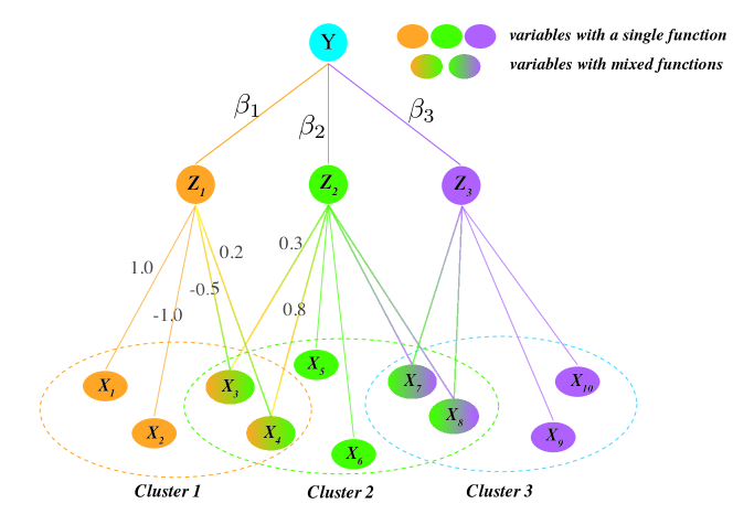
Figure 1 below gives an instance of Essential Regression. A response $Y$ depends on three latent factors $(Z_{1},Z_{2},Z_{3})$, which in turn are connected to $(X_{1},\ldots,X_{10})$. The measured variables $X_{1}$ and $X_{2}$ have only (100%) function $Z_{1}$. The $\pm$ 1 edge weights indicate that this function activates $X_{1}$ and inhibits $X_{2}$. Variable $X_{3}$ has mixed functions, $50\%$ is devoted to function $Z_{1}$, and the sign indicates that $Z_{1}$ is an inhibitor, while $30\%$ is devoted to function $Z_{2}$, an activator. The fact that the weights, in absolute value, do not sum up to 1 increases the model flexibility, by allowing free association between $X_{3}$ and other functions that are not explained by this model.

Figure 1: An illustrative example of Essential Regression

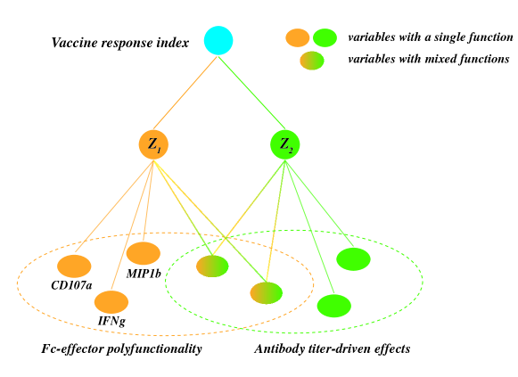
A similar, data-driven, figure is presented in Section 7, in which we show that the Essential Regression model fits the data collected in a new SIV-study (SIV is the non-human primate equivalent of HIV), and offers insights into immunological signatures driving the vaccine response. This example illustrates a scientifically-desirable way of modeling a response $Y$ directly at the function ($Z$) level, when the observed $X$-variables have either single or mixed functions.

1.2 Our contributions

Minimax adaptive estimation of $\beta$.

In Section 3, we construct a computationally tractable estimator of $\beta$. As part of the estimation procedure, the following unknown quantities are also estimated from the data, under the Essential Regression model: $A$, $I$, $K$, $\Sigma_{Z}:=\text{Cov}(Z)$, $\sigma^{2}:=\mathbb{E}[\varepsilon^{2}]$ and $\Gamma:=\text{Cov}(W)$. To benchmark the quality of our estimator we derive first, in Theorem 2 of Section 4.1 the minimax optimal rate of estimating $\beta$ in $\ell_{2}$-norm in an Essential Regression model. We show in Theorem 3 of Section 4.3 that the proposed estimator $\widehat{\beta}$ is minimax rate adaptive, up to logarithmic factors in $n$ and $p$. Our result uses the fact that only the estimation of the $|I|\times K$ sub-matrix $A_{I\,\begin{picture}(-1.0,1.0)(-0.5,-2.0)\circle*{2.3}\end{picture}\ }$, instead of the entire $p\times K$ matrix $A$, is involved in the construction of $\widehat{\beta}$. In Section 4.4 we introduce and discuss various competitors, including an estimator of $\beta$ that utilizes estimators of the full matrix $A$. These estimators are natural consequences of rewriting the identity for $\beta=\Sigma_{Z}^{-1}\text{Cov}(Z,Y)$, see (4), (5), (6), (24) and (26). We give insight into why these estimators are less efficient than the estimator proposed and studied, and confirm this in our simulation study in Section 6.

To estimate $I$ and $K$ we use the method proposed in Bing et al. (2019b), as it guarantees that we can consistently estimate $K$, without imposing any restrictions on our target for inference, $\beta$. Furthermore, this method also guarantees that $I\subseteq\widehat{I}\subseteq I\cup J_{1}$, where $J_{1}$ is an index set of what we term quasi-pure variables, defined formally in Section 4.2. As the name suggests, a quasi-pure variable is a measured $X$-variable that is very strongly associated with only one $Z_{k}$, while having very small, but non-zero, association with other latent factors. A signal strength assumption on the entries of $A$ would render $J_{1}=\varnothing$, which would simplify the analysis of $\widehat{\beta}$ considerably.

To maintain a flexible modeling framework, the proofs of all our results, rate optimality and asymptotic distribution, allow for the presence of quasi-pure variables, $J_{1}\neq\varnothing$, while controlling their relative number via Assumptions 3 and 3^′. The price to pay for considering a more realistic scenario is an increase in the technical difficulty of the proofs of Theorems 3 and 4 and Proposition 5, for instance in Lemmas 12, 15, 22, 32, 33, 34.

Inference for $\beta$: component-wise limiting distribution, asymptotic variance and its estimates.

Within various classes of identifiable factor models, and in the classical set-up $K$ and $p$ fixed, Anderson and Rubin (1956); Anderson and Amemiya (1988) proposed MLE-based estimators of the rows of identifiable loading factors $B$, in a generic factor model $U=BZ+E$. They pointed out that the asymptotic covariance matrix of the Gaussian limit of their estimators has a very involved expression, and left its derivation open.

In the regime $K$ fixed and $p\to\infty$, Bai and Li (2012) offered a solution to this problem, two decades later. They derived the asymptotic distribution, including the expression of the limiting covariance, of MLE-inspired estimators of the rows of $B$, under various identifiability restrictions on $B$, including a version of the conditions given in Section 4.5 below, corresponding to $I$ and $K$ known. Their proof uses a linearization argument, and requires $p\rightarrow\infty$ to establish that the corresponding remainder term converges in probability to zero. The practical implementation of the estimator involves an EM-type algorithm that is very sensitive to initialization, and becomes problematic in high dimensions. The estimation of the limiting covariance is not considered in their work.

Computationally feasible estimators of the rows of $B$, and in particular of the entries of $\beta$, with closed form, estimable, asymptotic variances continue to be lacking in the classical regime $K,p$ fixed, and also when both dimensions are allowed to grow. Furthermore, no results of this type have been established when $K$ and $I$ are unknown.

As our main contribution, we address these open questions in this work, via a unifying analysis, by studying the component-wise distribution of estimators of $\beta_{k}$, for $1\leq k\leq K$

Theorem 4 of Section 4.5 shows that the computationally tractable estimator proposed in Section 3 is asymptotically normal, with consistently estimable variance, under all scenarios of interest. A consistent estimator of this variance is given in Section 4.5 and its consistency is proved in Proposition 5. Table 1 below offers a snap shot of our asymptotic normality results, relative to existing results.

	$K$ and $I$ both known			$K$ and $I$ both unknown
	$K,p$ fixed	$K$ fixed, $p\to\infty$	$K,p\to\infty$	$K,p$ fixed	$K$ fixed, $p\to\infty$	$K,p\to\infty$
Existing results	Anderson and Rubin (1956), MLE estimator, no closed form of the asymptotic variance.	Bai and Li (2012), MLE-inspired estimator, computationally involved; closed form asymptotic variance $Q_{k}$ when $\lambda_{K}\asymp p$.	NA	NA	NA	NA
Theorem 4, Section 4.5	Computationally tractable $\widehat{\beta}_{k}$ and asymptotic variance $V_{k}$
	✓	$V_{k}$ reduces to $Q_{k}$ when $\lambda_{K}\to\infty$ and $\lambda_{K}\gtrsim({p}/{\sqrt{n}})\log(p\vee n)$.	✓	✓	✓	✓

Table 1: Asymptotically normal estimators of $\beta_{k}$ in a class of factor models: existing and new results (Theorem 4).

The quantity $\lambda_{K}:=\lambda_{K}(A\Sigma_{Z}A^{\top})$ quantifies the size of the signal in $X=AZ+W$. Theoretical analyses under the regime $p>n$ are performed under a conservative signal strength assumption, $\lambda_{K}\asymp p$, in the existing literature on factor models. See, for instance, (Chamberlain and Rothschild, 1983; Connor and Korajczyk, 1986; Bai and Ng, 2008; Bai, 2003; Fan et al., 2011, 2013). This includes results pertaining to inference on $\beta$ of Bai and Li (2012), which are most closely related to our work.

In Section 4.5 we prove that our proposed estimators of $\beta$ attain a Gaussian limit under a considerably relaxed condition, $\lambda_{K}\gtrsim{p/\sqrt{n}}$ (up to logarithmic $\log(p\vee n)$ factors), within a framework in which $K$ can grow as fast as $O(\sqrt{n}/\log(p\vee n))$. A technical discussion of this condition is provided in Section 4.2, and in Remark 3 of Section 4.5.

Table 1 offers a complete picture, to the best of our knowledge, of the existing literature on inference for $\beta$, under the modelling framework considered in this work. For completeness, we summarize in Remark 2 of Section 4.3, other approaches proposed in the literature for the selection of $K$, in other identifiable factor models. We summarize them, and state sufficient conditions for their consistency in Table 2.

For clarity of presentation, we give below the expressions of the limiting variances in the particular case when $\text{Cov}(W)=\tau^{2}\bf{I}_{p}$. By letting $\sigma^{2}=\mathbb{E}[\varepsilon^{2}]$, $\text{Cov}(W)=\tau^{2}\bf{I}_{p}$, $\Theta:=A\Sigma_{Z}$ and $\Theta^{+}=(\Theta^{\top}\Theta)^{-1}\Theta^{\top}$, the asymptotic variance derived in Bai and Li (2012), in the regime $K=O(1)$ and $\lambda_{K}\asymp p\rightarrow\infty$, is

$${Q_{k}=\left(\sigma^{2}+\tau^{2}\|\beta\|_{2}^{2}\right)\left[\Sigma_{Z}^{-1}\right]_{kk}}.$$

The assumption that $\lambda_{K}\asymp p$ is made in Bai and Li (2012) indirectly, as a consequence of their assumption (A) ($\Sigma_{Z}$ is positive definite and $K$ is fixed) and of their Assumption (C) ($\|A_{i\,\begin{picture}(-1.0,1.0)(-0.5,-2.0)\circle*{2.3}\end{picture}\ }\|_{2}\leq C$, $c\leq\Gamma_{ii}\leq C$ and $p^{-1}A^{\top}\Gamma^{-1}A$ converges to some positive definite matrix as $p\to\infty$), see page 438 of Bai and Li (2012).

The asymptotic variance of our proposed estimator, valid for all the regimes represented in Table 1 above, has the formula derived in Theorem 4 of Section 4.5,

$${V_{k}=\left(\sigma^{2}+{\tau^{2}\over m}\|\beta\|_{2}^{2}\right)\left[\left[\Sigma_{Z}^{-1}\right]_{kk}+\tau^{2}{\bf{e}}_{k}^{\top}\left(\Theta^{\top}\Theta\right)^{-1}{\bf{e}}_{k}\right]+{\tau^{4}\over m(m-1)}\sum_{a=1}^{K}\beta_{a}^{2}\sum_{i\in I_{a}}\left[{\bf{e}}_{k}^{\top}\Theta^{+}{\bf{e}}_{i}\right]^{2},}$$

where $\{{\bf{e}}_{1},\ldots,{\bf{e}}_{K}\}$ is the canonical basis of $\mathbb{R}^{K}$.

To contrast the two asymptotic variance expressions, we consider the common regime $K=O(1)$ and $p\rightarrow\infty$, in which case we note that the signal strength requirement under which our Theorem 4 is established reduces to $\lambda_{K}\gtrsim(p/\sqrt{n})\log(p\vee n)$. Theorem 4 shows that, in this case, if we further assume that $\lambda_{K}\to\infty$, the asymptotic variance of our estimator reduces to

$$V_{k}=\left(\sigma^{2}+{\tau^{2}\over m}\|\beta\|_{2}^{2}\right)\Omega_{kk},$$

and thus $\lim_{n\to\infty}Q_{k}/V_{k}\geq 1$. The two asymptotic variances coincide when $m=1$, which is the minimum identifiability requirement for a factor model with pure variables in which the pure variable set $I$ is known. Hence we recover, in this regime, the asymptotic variance derived in Bai and Li (2012), while at the same time relaxing their signal strength conditions required for this derivation.

As noted above, and as we prove formally in Theorem 4, the expression of the asymptotic variance $V_{k}$ is valid in all the regimes presented in this table. In particular, in the classical regime in which $K$ and $p$ do not vary with $n$, its derivation requires only $\lambda_{K}\gtrsim n^{-1/2}$.

In order to provide a unifying analysis, valid for both fixed and growing dimensions, we use the classical Lyapunov CLT for triangular arrays. The verification of the third moment condition of this theorem requires the lengthy, technical, derivations in Lemmas 21 and 24. Finally, although the expression of the asymptotic variance $V_{k}$ is involved, it can be estimated consistently for each $1\leq k\leq K$, by a computationally efficient estimator. This result is given in Proposition 5 of Section 4.5 and its proof, which requires considerable attention, is presented in Appendix F, followed by a list of the many technical lemmas used in this proof, Lemmas 26 – 34.

An application to regression on latent cluster centers

The identifiable factor model $X=AZ+W$ satisfying Assumption 1 in Section 2.1 below can be used to define, uniquely, overlapping clusters of the coordinates of $X$. The clusters are centered around the components of the latent vector $Z$, and $X$-variables in cluster $k$ have indices in the set $G_{k}:=\{j\in[p]:|A_{jk}|>0\},\ \text{for $1\leq k\leq K$}.$ A procedure for estimating consistently $K$ and the corresponding clusters has been developed recently in Bing et al. (2019b). With this interpretation, the Essential Regression framework can be employed for inference on the latent cluster centers. We show in Section 5 that although it may be tempting to replace the components of $Z$ by weighted averages of variables within a cluster, and subsequently regress $Y$ onto them, this procedure would not estimate $\beta$ in (1). However, we further show that this can be immediately corrected by regressing on the best linear predictor of $Z$ from these weighted averages. With this correction, we obtain exactly the estimator of $\beta$ constructed in Section 3, and the inferential tools developed in Section 4.5 can be used for inference in regression on unobserved, latent, cluster centers. In the context of the applications to biological data sets mentioned in Section 1.1, this will be inference at the biological signature level, as illustrated in Section 7.

1.3 Organization of the paper

The rest of the paper is organized as follows.

Section 2 gives a set of modeling assumptions under which the model given by (1) and (2) is identifiable. Section 2.1 introduces and discusses these assumptions, including parameter interpretability. Section 2.2 shows that our central parameter, $\beta$, along with other important parameters, is identifiable.

Section 3 introduces our proposed estimator $\widehat{\beta}$ of $\beta$. Section 4.4 discusses other natural estimators, and explains why they should be expected to have inferior theoretical and practical perfomance relative to $\widehat{\beta}$. The numerical performance of these alternate estimators is presented in Section 6.

The performance of estimators of $\beta$ in factor regression models satisfying Assumption 1 is benchmarked in Section 4.1. Theorem 2 provides the minimax lower bound for estimating $\beta$ in this class of models, with respect to the $\ell_{2}$ loss.

Section 4.3 shows that the estimator $\widehat{\beta}$ proposed in Section 3 is $\ell_{2}$-norm consistent, and minimax-rate adaptive, under assumptions collected in Section 4.2.

Section 4.5 is devoted to the component-wise asymptotic normality of $\widehat{\beta}$ and to the estimation of the asymptotic variance, as well as to a comparison with existing literature.

Section 5 presents an application of the framework, methodology and theory developed in previous sections to regression on latent cluster centers, when the clusters are allowed to overlap.

Section 6 verifies numerically our theoretical results. Section 7 shows how our methodology can be used to make inference on unobserved, latent, immunological modules, using a data set collected during a study on the effectiveness of a new SIV-type vaccine.

All proofs are deferred to the supplement. Appendix B gives the proofs of Proposition 1 and Theorem 2, on identification and minimax lower bounds, respectively. Appendix C provides necessary preliminary results, and could be skipped at first reading. The proof of Theorem 3 concerning the convergence rates of $\widehat{\beta}$ is given in Appendix D. The proof of Theorem 4 on the asymptotic normality of $\widehat{\beta}$ is given in Appendix E, while Proposition 5 on consistent estimation of the asymptotic variance $V_{k}$ is proved in Appendix F.

1.4 Notation

For any positive integer $q$, we let $[q]=\{1,2,\ldots,q\}$. For two numbers $a$ and $b$, we write $a\vee b:=\max\{a,b\}$ and $a\wedge b:=\min\{a,b\}$. For a set $S$, we use $|S|$ to denote its cardinality. We use $\mathcal{H}_{d}$ to denote the set of all $d\times d$ signed permutation matrices and $\mathcal{S}^{d-1}$ to represent the space of the unit vectors in $\mathbb{R}^{d}$. We denote by ${\bf{I}}_{d}$ the $d\times d$ identity matrix, by $\bm{1}_{d}$ the $d$-dimensional vector with entries equal to $1$ and by $\{{\bf{e}}_{j}\}_{1\leq j\leq d}$ the canonical basis in $\mathbb{R}^{d}$. For a generic vector $v$, we let $\|v\|_{q}=\left(\sum_{i}|v_{i}|^{q}\right)^{1/q}$ denote its $\ell_{q}$ norm for $1\leq q<\infty$. We also write $\|v\|_{\infty}=\max_{i}|v_{i}|$ and $\|v\|_{0}=|\textrm{supp}(v)|$. Let $Q$ be any matrix. We use $\|Q\|_{{\rm op}}=\sup_{v\in\mathcal{S}^{d-1}}\|Qv\|$ and $\|Q\|_{\infty}=\max_{i,j}|Q_{ij}|$ for its operator norm and element-wise maximum norm, respectively. For a symmetric matrix $Q\in\mathbb{R}^{d\times d}$, we denote by $\lambda_{k}(Q)$ its $k$th largest eigenvalue for $k\in[d]$. For a positive semi-definite symmetric matrix, we will frequently use the fact that $\lambda_{1}(Q)=\|Q\|_{{\rm op}}$. For an arbitrary real valued matrix $M$, we let $\sigma_{K}(M)$ denote its $k$th singular value (in decreasing order).

For any two sequences $a_{n}$ and $b_{n}$, $a_{n}\lesssim b_{n}$ stands for there exists constant $C>0$ such that $a_{n}\leq Cb_{n}$. We write $a_{n}\asymp b_{n}$ if $a_{n}\lesssim b_{n}$ and $b_{n}\lesssim a_{n}$. We also use $a_{n}=o(b_{n})$ to denote $a_{n}/b_{n}\to 0$ as $n\to\infty$.

2 Modeling assumptions and identifiability

2.1 Modeling assumptions

We begin by formalizing and explaining the set of model identifiability assumptions that will be used in this work.

Assumption 1.

1. $\|A_{j\,\begin{picture}(-1.0,1.0)(-0.5,-2.0)\circle*{2.3}\end{picture}\ }\|_{1}\leq 1$ for all $j\in[p]$.

2. For every $k\in[K]$, there exists at least two $j\neq\ell\in[p]$, such that $|A_{j\,\begin{picture}(-1.0,1.0)(-0.5,-2.0)\circle*{2.3}\end{picture}\ }|=|A_{\ell\,\begin{picture}(-1.0,1.0)(-0.5,-2.0)\circle*{2.3}\end{picture}\ }|={\bf{e}}_{k}$.

3. $\Sigma_{Z}:=\text{Cov}(Z)$ is positive definite. There exists a constant $\nu>0$ such that

   $$\min_{1\leq a<b\leq K}\Bigl{(}\left[\Sigma_{Z}\right]_{aa}\wedge\left[\Sigma_{Z}\right]_{bb}-\left|\left[\Sigma_{Z}\right]_{ab}\right|\Bigr{)}>\nu.$$

In (A1), the absolute value is taken entry-wise and we use $\{{\bf{e}}_{1},\ldots,{\bf{e}}_{K}\}$ to denote the canonical basis in $\mathbb{R}^{K}$. For future reference, we denote the index set corresponding to pure variables as

$$I=\bigcup_{k=1}^{K}I_{k},\qquad I_{k}=\left\{i\in[p]:|A_{i\,\begin{picture}(-1.0,1.0)(-0.5,-2.0)\circle*{2.3}\end{picture}\ }|={\bf{e}}_{k}\right\}.$$ (3)

Its complement set is called the non-pure variable set $J:=[p]\setminus I$.

Assumption 1 guarantees that $A$ and $\Sigma_{Z}$ are identifiable, up to signed permutations (Bing et al., 2019b, Theorem 2). We refer to the second assumption (A1) as the pure variable assumption. It states that every $Z_{k}$, $1\leq k\leq K$, must have at least two components of $X$, the pure variables, solely associated with it, up to additive noise with possibly different variance levels. An in-depth comparison with the rich literature on factor models of type (2) and a detailed explanation of assumptions (A0) – (A2) can be found in Bing et al. (2019b), and thus we only offer a brief set of comments here.

If $A\Sigma_{Z}A^{T}$ is identifiable, we show in Corollary 6 in Appendix A that $A$ and $\Sigma_{Z}$ are identifiable up to signed permutations under Assumption 1, but when (A1) is relaxed to

(A1’) For each $$k\in[K] i\in[p] A_{i\cdot}={\bf{e}}_{k}$$, there exists at least one index such that .

However, the existing conditions under which $A\Sigma_{Z}A^{T}$ can be identified from the decomposition $\Sigma=A\Sigma_{Z}A^{T}+\Gamma$ can be incompatible with factor models with pure variables, for instance the incoherence condition in Chandrasekaran et al. (2009), or can be very stringent growth conditions on the eigenvalues of $A\Sigma_{Z}A^{T}$. For an instance of the latter we refer to Fan et al. (2013); Bai and Ng (2002) and also to Table 2 below. These difficulties can be bypassed under (A1) of Assumption 1, using the approach taken in Bing et al. (2019b), which does not rely on separating out $A\Sigma_{Z}A^{T}$ from $\Sigma$ in the first step. In Assumption 1, (A0), we set the scale to 1 to aid the interpretation of matrix $A$ as a cluster membership matrix, and thus view the model $X=AZ+W$ as a latent clustering model, following Bing et al. (2019b). The equality between the weights of two pure variables, $|A_{j\cdot}|=|A_{\ell\cdot}|={\bf{e}}_{k}$ has been relaxed in a recent work, (Bing et al., 2020), but under a slightly different scaling condition than (A0), and we do not pursue that approach here.

Furthermore, we mention, for completeness, that a more rigid form of assumption (A1’), specifically

(A1”) For each $$k\in[K] i\in[p] A_{i\cdot}={\bf{e}}_{k}$$, there exists a known index such that ,

has had a long history, as it is one of the few “user-interpretable” parametrizations of $A$ that eliminates the rotation ambiguity of the latent factors. In psychology, the “pure” variables induced by the parametrization are called factorially simple items McDonald (1999). A similar condition on $A$ can be traced back to the econometrics literature, and an early reference is Koopmans and Reiersol (1950), further discussed in Anderson and Rubin (1956), who called it “zero elements (of $A$) in specified positions”. We refer to Koopmans and Reiersol (1950); Anderson and Rubin (1956); Thurstone (1931) for more examples in psychology, sociology, etc. This parametrization is also called the errors-in-variable parametrization and has wide applications in structural equation models, see, Joreskog (1970a, b). The more recent review paper Yalcin and Amemiya (2001), and the references therein, provide a nice overview of many other concrete applications that support interest in factor models under a parametrization of this type. We provide another example below.

In the context of Assumption 1, we interpret the entries in $A$ as (signed) mixture weights. Under model (1), each $X_{j}$ is a signed mixture of $Z_{1},\ldots,Z_{K}$, according to these weights. This assumption, which is sufficient for identifiability, is also a a desirable modelling assumption.

As an illustration, assume that $X\in\mathbb{R}^{p}$ contains gene-level measurements, and that $Z\in\mathbb{R}^{K}$ corresponds to their biological functions. Then, (A0) enables, in this example, to associate a gene with multiple biological functions, in different proportions per function. The inequality sign in (A0) further allows some genes not to be associated with any of the functions captured by this model, thereby increasing the robustness of the model. The second requirement, (A1), simply says that the measured $X_{j}$ and $X_{\ell}$ have the same biological function $Z_{k}$, and only that function. We considered signed mixtures to increase the flexibility of the model. In this example, signs correspond to the nature of the function. For instance, if gene $X_{j}$ activates a signaling pathway, and $Z_{k}$ has positive sign, then $Z_{k}$ has a function associated with the activation of this pathway, whereas a negative sign indicates a function associated with its inhibition.

Assumption (A2) allows us to depart from the widely used, and restrictive, assumption of independence among the latent factors. We require the variability of the factors to be strictly larger than that between factors. This implies the minimal desideratum that the factors be different.

We first discuss the identifiability of $\beta$ in Section 2.2. Then in Section 3, we propose our estimator of $\beta$ which uses its identifiability constructively.

2.2 Identifiability of $\beta$: a constructive approach

Under model (1), we have $Y=Z^{\top}\beta+\varepsilon$, and thus the coefficient $\beta$ satisfies

$$\beta=[\text{Cov}(Z)]^{-1}\text{Cov}(Z,Y)=\Sigma_{Z}^{-1}\text{Cov}(Z,Y).$$ (4)

Since model (2) and Assumption 1 imply $\text{Cov}(Z,Y)=(A^{\top}A)^{-1}A^{\top}\text{Cov}(X,Y)$, we have

$$\beta ~{}=~{}\Sigma_{Z}^{-1}(A^{\top}A)^{-1}A^{\top}\text{Cov}(X,Y)$$ (5)

$$~{}=~{}(\Theta^{\top}\Theta)^{-1}\Theta^{\top}\text{Cov}(X,Y)$$ (6)

with $\Theta=A\Sigma_{Z}$. Therefore, $\beta$ is uniquely defined whenever $\Theta$ is unique. By partitioning the $p\times K$ matrix $A$ as $A_{I\,\begin{picture}(-1.0,1.0)(-0.5,-2.0)\circle*{2.3}\end{picture}\ }\in\mathbb{R}^{|I|\times K}$ and $A_{J\,\begin{picture}(-1.0,1.0)(-0.5,-2.0)\circle*{2.3}\end{picture}\ }\in\mathbb{R}^{|J|\times K}$ corresponding to $I$ and $J$, respectively, model (2) and Assumption 1 imply the following decomposition of $\Sigma$,

$$\Sigma=\begin{bmatrix}\Sigma_{II}&\Sigma_{IJ}\\ \Sigma_{JI}&\Sigma_{JJ}\end{bmatrix}=\begin{bmatrix}A_{I\,\begin{picture}(-1.0,1.0)(-0.5,-2.0)\circle*{2.3}\end{picture}\ }\Sigma_{Z}A_{I\,\begin{picture}(-1.0,1.0)(-0.5,-2.0)\circle*{2.3}\end{picture}\ }^{\top}&A_{I\,\begin{picture}(-1.0,1.0)(-0.5,-2.0)\circle*{2.3}\end{picture}\ }\Sigma_{Z}A_{J\,\begin{picture}(-1.0,1.0)(-0.5,-2.0)\circle*{2.3}\end{picture}\ }^{\top}\vspace{2mm}\\ A_{J\,\begin{picture}(-1.0,1.0)(-0.5,-2.0)\circle*{2.3}\end{picture}\ }\Sigma_{Z}A_{I\,\begin{picture}(-1.0,1.0)(-0.5,-2.0)\circle*{2.3}\end{picture}\ }^{\top}&A_{J\,\begin{picture}(-1.0,1.0)(-0.5,-2.0)\circle*{2.3}\end{picture}\ }\Sigma_{Z}A_{J\,\begin{picture}(-1.0,1.0)(-0.5,-2.0)\circle*{2.3}\end{picture}\ }^{\top}\end{bmatrix}+\begin{bmatrix}\Gamma_{II}&\\ &\Gamma_{JJ}\end{bmatrix}.$$

In particular, we have $\Sigma_{II}=A_{I\,\begin{picture}(-1.0,1.0)(-0.5,-2.0)\circle*{2.3}\end{picture}\ }\Sigma_{Z}A_{I\,\begin{picture}(-1.0,1.0)(-0.5,-2.0)\circle*{2.3}\end{picture}\ }^{\top}+\Gamma_{II}$ and

$$\Theta=A\Sigma_{Z}=\left(\Sigma_{\,\begin{picture}(-1.0,1.0)(-0.5,-2.0)\circle*{2.3}\end{picture}\ I}-\Gamma_{\,\begin{picture}(-1.0,1.0)(-0.5,-2.0)\circle*{2.3}\end{picture}\ I}\right)A_{I\,\begin{picture}(-1.0,1.0)(-0.5,-2.0)\circle*{2.3}\end{picture}\ }^{\top}(A_{I\,\begin{picture}(-1.0,1.0)(-0.5,-2.0)\circle*{2.3}\end{picture}\ }^{\top}A_{I\,\begin{picture}(-1.0,1.0)(-0.5,-2.0)\circle*{2.3}\end{picture}\ })^{-1}.$$ (7)

The uniqueness of $\Theta$ is thus implied by that of $A_{I\,\begin{picture}(-1.0,1.0)(-0.5,-2.0)\circle*{2.3}\end{picture}\ }$ and $\Sigma_{Z}$. Theorem 1 in Bing et al. (2019b) shows that, under Assumption 1, the matrices $A_{I\,\begin{picture}(-1.0,1.0)(-0.5,-2.0)\circle*{2.3}\end{picture}\ }$ and $\Sigma_{Z}$ can be uniquely determined, up to a signed permutation matrix $P$, from $\Sigma:=\text{Cov}(X)$. As a result, $\Theta$ can also be recovered from (7) up to $P^{\top}$, hence $\beta$ is identifiable from (6) up to $P^{\top}$. We remark that the permutation matrix $P$ will not affect either inference or prediction. Indeed, writing $\widetilde{A}=AP$, $\widetilde{Z}=P^{\top}Z$ and $\widetilde{\beta}=P^{\top}\beta$, one still has $Y=\widetilde{Z}^{\top}\widetilde{\beta}+\varepsilon$ and $X=\widetilde{A}\widetilde{Z}+W$. We summarize the identifiability of $\beta$ in the proposition below. Its proof can be found in Appendix B.1.

Proposition 1.

Under models (1) – (2) and Assumption 1, the quantities $\Sigma$ and $\text{Cov}(X,Y)$ define $\beta$ uniquely, via (6) and (7), up to a signed permutation matrix.

Our estimator, given in the next section, is based on the representations (6) and (7), followed by appropriate plug-in estimators.

3 Estimation of $\beta$

We assume that the data consists of $n$ independent observations $(X_{1},Y_{1}),\ldots,(X_{n},Y_{n})$ that satisfy model (1) and (2). We write $\mathbf{X}:=(X_{1},\ldots,X_{n})^{\top}$ for the observed $n\times p$ data matrix and $\mathbf{y}:=(Y_{1},\ldots,Y_{n})^{\top}$ for the observed response vector. Let $\widehat{\Sigma}=n^{-1}\sum_{i=1}^{n}X_{i}X_{i}^{\top}$ denote the sample covariance matrix. Motivated by equations (6) and (7), we consider the plug-in estimator of $\beta$ via the following steps:

1. Obtain estimates $\widehat{K}$ and $\{\widehat{I}_{1},\cdots,\widehat{I}_{\widehat{K}}\}$ from $\widehat{\Sigma}$ with tuning parameter $\delta$ by using Algorithm 1 in Bing et al. (2019b). For the reader’s convenience, we state the procedure in Algorithm 1 below.

2. Next, for each $a\in[\widehat{K}]$ and $b\in[\widehat{K}]\setminus\{a\}$, we compute

   $$[\widehat{\Sigma}_{Z}]_{aa}=\frac{1}{|\widehat{I}_{a}|(|\widehat{I}_{a}|-1)}\sum_{i\neq j\in\widehat{I}_{a}}|\widehat{\Sigma}_{ij}|,\quad~{}[\widehat{\Sigma}_{Z}]_{ab}=\frac{1}{|\widehat{I}_{a}||\widehat{I}_{b}|}\sum_{i\in\widehat{I}_{a},j\in\widehat{I}_{b}}\widehat{A}_{ia}\widehat{A}_{ib}\widehat{\Sigma}_{ij},$$ (8)

   to form the estimator $\widehat{\Sigma}_{Z}$ of $\Sigma_{Z}$. Furthermore, the estimation of $A_{I\,\begin{picture}(-1.0,1.0)(-0.5,-2.0)\circle*{2.3}\end{picture}\ }$ follows the procedure in Bing et al. (2019b). For each $k\in[\widehat{K}]$ and the estimated pure variable set $\widehat{I}_{k}$,

   Pick an element $$i\in\widehat{I}_{k} \widehat{A}_{i\,\begin{picture}(-1.0,1.0)(-0.5,-2.0)\circle*{2.3}\end{picture}\ }={\bf{e}}_{k}$$ at random, and set ; (9)

   For the remaining $$j\in\widehat{I}_{k}\setminus\{i\} \widehat{A}_{j\,\begin{picture}(-1.0,1.0)(-0.5,-2.0)\circle*{2.3}\end{picture}\ }=\textrm{sign}(\widehat{\Sigma}_{ij})\cdot{\bf{e}}_{k}$$, set . (10)

3. Estimate $\Gamma_{\,\begin{picture}(-1.0,1.0)(-0.5,-2.0)\circle*{2.3}\end{picture}\ I}$ by $\widehat{\Gamma}_{{\,\begin{picture}(-1.0,1.0)(-0.5,-2.0)\circle*{2.3}\end{picture}\ \widehat{I}}}$ with

   $$\widehat{\Gamma}_{ii}=\widehat{\Sigma}_{ii}-\widehat{A}_{i\,\begin{picture}(-1.0,1.0)(-0.5,-2.0)\circle*{2.3}\end{picture}\ }^{\top}\widehat{\Sigma}_{Z}\widehat{A}_{i\,\begin{picture}(-1.0,1.0)(-0.5,-2.0)\circle*{2.3}\end{picture}\ },\quad\forall\ i\in\widehat{I},\qquad\widehat{\Gamma}_{ji}=0,\quad\forall\ j\neq i.$$ (11)

4. Compute

   $$\widehat{\Theta}=\left(\widehat{\Sigma}_{\,\begin{picture}(-1.0,1.0)(-0.5,-2.0)\circle*{2.3}\end{picture}\ \widehat{I}}-\widehat{\Gamma}_{{\,\begin{picture}(-1.0,1.0)(-0.5,-2.0)\circle*{2.3}\end{picture}\ \widehat{I}}}\right)\widehat{A}_{{\widehat{I}\,\begin{picture}(-1.0,1.0)(-0.5,-2.0)\circle*{2.3}\end{picture}\ }}\left(\widehat{A}_{{\widehat{I}\,\begin{picture}(-1.0,1.0)(-0.5,-2.0)\circle*{2.3}\end{picture}\ }}^{\top}\widehat{A}_{{\widehat{I}\,\begin{picture}(-1.0,1.0)(-0.5,-2.0)\circle*{2.3}\end{picture}\ }}\right)^{-1}.$$ (12)

   Provided that $\widehat{\Theta}^{\top}\widehat{\Theta}$ is non-singular, estimate $\beta$ by

   $$\widehat{\beta}=\left(\widehat{\Theta}^{\top}\widehat{\Theta}\right)^{-1}\widehat{\Theta}^{\top}{1\over n}\mathbf{X}^{\top}\mathbf{y}.$$ (13)

Algorithm 1 Estimate the partition of the pure variables $\mathcal{I}$ by $\widehat{\mathcal{I}}$

1:procedure PureVar($\widehat{\Sigma}$, $\delta$)

2:     $\widehat{\mathcal{I}}\leftarrow\varnothing$.

3:     for all $i\in[p]$ do

4:         $\widehat{I}^{(i)}\leftarrow\bigl{\{}l\in[p]\setminus\{i\}:\max_{j\in[p]\setminus\{i\}}|\widehat{\Sigma}_{ij}|\leq|\widehat{\Sigma}_{il}|+2\delta\bigr{\}}$

5:         $Pure(i)\leftarrow True$.

6:         for all $j\in\widehat{I}^{(i)}$ do

7:              if $\bigl{|}|\widehat{\Sigma}_{ij}|-\max_{k\in[p]\setminus\{j\}}|\widehat{\Sigma}_{jk}|\bigr{|}>2\delta$ then

8:                  $Pure(i)\leftarrow False$,

9:                  break                        

10:         if $Pure(i)$ then

11:              $\widehat{I}^{(i)}\leftarrow\widehat{I}^{(i)}\cup\{i\}$

12:              $\widehat{\mathcal{I}}\leftarrow$ Merge($\widehat{I}^{(i)},\ \widehat{\mathcal{I}}$)               

13:     return $\widehat{\mathcal{I}}$ and $\widehat{K}$ as the number of sets in $\widehat{\mathcal{I}}$

14:

15:function Merge($\widehat{I}^{(i)}$, $\widehat{\mathcal{I}}$)

16:     for all $G\in\widehat{\mathcal{I}}$ do $\triangleright$ $\widehat{\mathcal{I}}$ is a collection of sets

17:         if $G\cap\widehat{I}^{(i)}\neq\varnothing$ then

18:              $G\leftarrow G\cap\widehat{I}^{(i)}$ $\triangleright$ Replace $G\in\widehat{\mathcal{I}}$ by $G\cap\widehat{I}^{(i)}$

19:              return $\widehat{\mathcal{I}}$               

20:     $\widehat{I}^{(i)}\in\widehat{\mathcal{I}}$ $\triangleright$ add $\widehat{I}^{(i)}$ in $\widehat{\mathcal{I}}$

21:     return $\widehat{\mathcal{I}}$

The above procedure requires a single tuning parameter $\delta$, and that $K<n$. The theoretical order of $\delta$ is given in (17) of Section 4.2 under the sub-Gaussian distributional assumptions. A practical data-driven procedure of selecting $\delta$ is stated in Appendix H. We show in Section 5 that $\widehat{\beta}$ coincides with the ordinary least squares estimator that minimizes $\|\mathbf{y}-\widehat{\mathbf{Z}}\beta\|_{2}^{2}$ over $\beta$, based on an appropriately constructed predictor $\widehat{\mathbf{Z}}$ of the latent data matrix $\mathbf{Z}:=(Z_{1},\ldots,Z_{n})^{\top}$. We prove in Theorem 3 of Section 4.3 that $\widehat{\Theta}^{\top}\widehat{\Theta}$ is non-singular with high probability. In practice, in case that $\widehat{\Theta}^{\top}\widehat{\Theta}$ is singular or ill-conditioned, we propose to invert $\widehat{\Theta}^{\top}\widehat{\Theta}+t\cdot{\bf I}_{\widehat{K}}$ instead, for any small $t>0$.

In Section 4.4 we discuss other possible estimators based on the alternative representations of $\beta$ given in (4), (5) and (6).

4 Statistical guarantees

4.1 Minimax lower bounds for estimators of $\beta$ in Essential Regression

To benchmark our estimator of $\beta$, we derive the minimax optimal rate of $\|\widehat{\beta}-\beta\|_{2}$ over the parameter space $(\beta,\Sigma_{Z},A)\in\mathcal{S}(R,m)$ with

$$\mathcal{S}(R,m):=\big{\{}(\beta,\Sigma_{Z},A):\ \|\beta\|_{2}\leq R,\ C_{\min}\leq\lambda_{\min}(\Sigma_{Z})\leq\lambda_{\max}(\Sigma_{Z})\leq C_{\max},$$

$$A\text{ satisfies Assumption \ref{ass_model} with }\min_{k}|I_{k}|=m\big{\}},$$

where $I_{k}$ is defined in (3). For the purpose of the minimax result, it suffices to consider the joint distribution of $(X,Y)$ as

$$\begin{bmatrix}X\\ Y\end{bmatrix}\sim N_{p+1}\left(0,\begin{bmatrix}A\Sigma_{Z}A^{\top}+\tau^{2}{\bf{I}}_{p}&A\Sigma_{Z}\beta\\ \beta^{\top}\Sigma_{Z}A^{\top}&\beta^{\top}\Sigma_{Z}\beta+\sigma^{2}\end{bmatrix}\right)$$ (14)

for $(\beta,\Sigma_{Z},A)\in\mathcal{S}(R,m)$ and some positive constants $\sigma^{2}$ and $\tau^{2}$.

Theorem 2.

Let $K\leq\bar{c}(R^{2}\vee m)n$ for some positive constant $\bar{c}$. Let $(X_{1},Y_{1}),\ldots,(X_{n},Y_{n})$ be i.i.d. random variables from the normal distribution in (14). Then, there exist constants $c^{\prime}>0$, $c^{\prime\prime}\in(0,1]$ depending only on $\bar{c}$, $C_{\max}$, $C_{\min}$, $\sigma^{2}$ and $\tau^{2}$, such that

$$\inf_{\widehat{\beta}}\sup_{(\beta,\Sigma_{Z},A)\in\mathcal{S}(R,m)}\mathbb{P}\left\{\|\widehat{\beta}-\beta\|_{2}\geq c^{\prime}\left(1\vee{R\over\sqrt{m}}\right)\cdot\sqrt{K\over n}\right\}\geq c^{\prime\prime}.$$ (15)

The inf is taken over all estimators $\widehat{\beta}$ of $\beta$.

Proof.

The proof is deferred to Appendix B.2. It uses the classical technique in Tsybakov (2009) for proving minimax lower bounds. After carefully constructing a set of “hypotheses” of $\beta$, we observe that the Kullback-Leibler (KL) divergence between joint distributions of $(X,Y)$ parametrized by two hypotheses of $\beta$ can be calculated from the log ratio of corresponding conditional densities of $Y|X$. This observation greatly simplifies the proof. ∎

The factor $\sqrt{K/n}$ in (15) is the standard minimax rate of estimation in linear regression with observed $Z$ and sub-Gaussian errors. The factor multiplying it can be viewed as the price to pay for not observing $Z$. It quantifies the trade-off between not observing $Z$, with strength $\|\beta\|_{2}$, and the number of times, given by $m=\min_{k}|I_{k}|$, each component of $Z$ is partially observed, up to additive error. The ratio $\|\beta\|_{2}/\sqrt{m}$ indicates that, under the Essential Regression framework, the fact that $Z$ is not observed can be alleviated by the existence of pure variables, and the quality of estimation is expected to increase as $m$ increases. Theorem 2 above shows that, from the point of view of estimating $\beta$ consistently in Essential Regression, the number of factors $K$ can grow with $n$, a scenario not treated in the more classical factor regression literature. It also reveals that, as in the classical regression set-up, although $K$ can grow with $n$ in Essential Regression, consistent estimation of unstructured $\beta$ cannot be guaranteed when $K>n$. This will be treated in follow-up work.

To the best of our knowledge, the minimax lower bound established above is a new result in the factor regression model literature and it is interesting to place our results in a broader, related, context. For this, note that under the Essential Regression framework, if $I$ and $A_{I\,\begin{picture}(-1.0,1.0)(-0.5,-2.0)\circle*{2.3}\end{picture}\ }$ were known, the pure variable assumption implies

$$Y=Z^{\top}\beta+\varepsilon,\qquad\bar{X}_{I}=Z+\bar{W}_{I}$$ (16)

with $\bar{X}_{I}:=(A_{I\,\begin{picture}(-1.0,1.0)(-0.5,-2.0)\circle*{2.3}\end{picture}\ }^{\top}A_{I\,\begin{picture}(-1.0,1.0)(-0.5,-2.0)\circle*{2.3}\end{picture}\ })^{-1}A_{I\,\begin{picture}(-1.0,1.0)(-0.5,-2.0)\circle*{2.3}\end{picture}\ }^{\top}X_{I}$ and $\bar{W}_{I}:=(A_{I\,\begin{picture}(-1.0,1.0)(-0.5,-2.0)\circle*{2.3}\end{picture}\ }^{\top}A_{I\,\begin{picture}(-1.0,1.0)(-0.5,-2.0)\circle*{2.3}\end{picture}\ })^{-1}A_{I\,\begin{picture}(-1.0,1.0)(-0.5,-2.0)\circle*{2.3}\end{picture}\ }^{\top}W_{I}$. Model (16) becomes an instance of an errors in variables model where the covariance structure of the error term $\bar{W}_{I}$ is diagonal. The minimax optimal lower bound for estimating $\beta$ in such models has been derived recently in Belloni et al. (2017), under sparsity assumptions on $\beta$. In the particular case of non-sparse $\beta$, which we treat here, their lower bound agrees with that given by our Theorem 2, although their bound is derived over a larger class, and can only be compared with (15) when $I$ is known. The closest result to that of Theorem 2 is the minimax lower bound on rows of $A$ bounded in $\ell_{1}$ norm, and has been derived in Bing et al. (2019b). We complement this here, in the latent factor regression context, by providing a minimax lower bound on $\beta$ with a $\ell_{2}$ norm allowed to increase with $n$.

4.2 Assumptions

In this section we collect the assumptions under which we evaluate the performance of our proposed estimator $\widehat{\beta}$.

We first make the following distributional specifications for $\varepsilon$, $W$ and $Z$ defined in model (1):

Assumption 2.

Let $\gamma_{\varepsilon},\gamma_{w},\gamma_{z}$ and $B_{z}$ be positive finite constants. Assume $\varepsilon$ is $\gamma_{\varepsilon}$-sub-Gaussian and $W$ has independent $\gamma_{w}$-sub-Gaussian entries. Further assume $\|\Sigma_{Z}\|_{\infty}\leq B_{z}$ and the random vector $\Sigma_{Z}^{-{1/2}}Z$ is $\gamma_{z}$-sub-Gaussian.

The quality of our estimator $\widehat{\beta}$ given by (13) depends on how well we estimate $K$, $I$, its partition $\{I_{k}\}_{1\leq k\leq K}$, as well as $\Theta$. Our goal is to estimate $K$ consistently, under minimal assumptions. However, consistent estimation of the partition requires a stronger set of assumptions that we would like to avoid. We introduce and discuss below a set of assumptions under which the partition is recovered sufficiently well for the purpose of inference on $\widehat{\beta}$.

Assumption 2 implies that $X_{j}$ is $\gamma_{x}$-sub-Gaussian with $\gamma_{x}=(\gamma_{z}\sqrt{B_{z}}+\gamma_{w})$, as shown in Lemma 9 in Appendix C.3, and it is well known (see, for instance, (Bien et al., 2016, Lemma 1)) that in this case,

$$\mathbb{P}\left\{\max_{1\leq j<\ell\leq p}|\widehat{\Sigma}_{j\ell}-\Sigma_{j\ell}|\leq\delta\right\}\geq 1-(p\vee n)^{-c^{\prime}}$$ (17)

with $\delta=c\sqrt{\log(p\vee n)/n}$, for some constant $c^{\prime}>0$ and $c=c(\gamma_{x})>0$ sufficiently large.

Under Assumptions 1 and 2, and when $\log p\leq c^{\prime\prime}n$ for some constant $c^{\prime\prime}>0$, Bing et al. (2019b) provides an algorithm for estimating $K$ and $I$, and prove in their Theorem 3 the following:

1. $\widehat{K}=K$;

2. $I_{k}\subseteq\widehat{I}_{\pi(k)}\subseteq I_{k}\cup J_{1}^{k}$, for all $k\in[K]$,

where $\pi:[K]\rightarrow[K]$ is a permutation and $J_{1}^{k}:=\{j\in J:|A_{jk}|\geq 1-4\delta/\nu\}$ with constant $\nu$ defined in Assumption 1 of Section 2.1 above.

Since we do not impose any separation condition between the pure variable rows $A_{I\,\begin{picture}(-1.0,1.0)(-0.5,-2.0)\circle*{2.3}\end{picture}\ }$ and the remaining rows in $A_{J\,\begin{picture}(-1.0,1.0)(-0.5,-2.0)\circle*{2.3}\end{picture}\ }$, the sets $\{J_{1}^{k}\}_{k=1}^{K}$ are typically not empty, and as formalized in (2) above, we cannot expect to recover $I$ perfectly in the presence of quasi-pure variables with indices belonging to the set $J_{1}\coloneqq\bigcup_{k=1}^{K}J_{1}^{k}$. Indeed, when $\log p=o(n)$, for any $j\in J_{1}^{k}$ we have $|A_{jk}|\approx 1$ and $A_{jk^{\prime}}\approx 0$ for any $k^{\prime}\neq k$, so variables corresponding to $J_{1}^{k}$ are very close to the pure variables in $I_{k}$, and possibly indistinguishable from one another, in finite samples.

While allowing for $J_{1}\neq\varnothing$ increases the flexibility of the model, it also poses significant technical difficulties in the analysis of the asymptotic distribution of $\widehat{\beta}_{k}$, for each $k$, evidenced in the proofs of Theorem 3, Theorem 4 and Proposition 5. Nevertheless, the limiting distribution can still be derived when $|J_{1}|$ is small relative to $|I|$. The influence of the misclassified $X$-variables with entries in $J_{1}$ becomes negligible in both the finite sample rate analysis of $\widehat{\beta}$ provided in Section 4.3 and the asymptotic analysis of Section 4.5 under the condition given below. We introduce

$$\bar{\rho}^{2}=\sum_{k=1}^{K}\left(\frac{|J_{1}^{k}|}{|I_{k}|+|J_{1}^{k}|}\right)^{2}$$ (18)

to quantify the influence of quasi-pure variables on the quality of our estimation. Theorem 3 shows that optimal estimation of $\beta$ is possible in the presence of quasi-pure variables as long as their number is negligible relative to the number of pure variables in the same group, in that the following assumption holds.

Assumption 3.

3 The overall proportion $\bar{\rho}^{2}$ satisfies $m\bar{\rho}^{2}=O(1)$ with $m:=\min_{k\in[K]}|I_{k}|$.

We briefly discuss this assumption below. Let $s\leq K$ be the number of factors that have quasi-pure variables, that is,

$$s=|S|,\quad S=\{1\leq k\leq K:|J_{1}^{k}|\geq 1\}.$$

1. Note that, by (18), we have $\bar{\rho}^{2}\leq s$, and therefore $m\bar{\rho}^{2}\leq ms$. Thus, if both $s$ (and in particular $K$, when $s=K$) and $m$ remain bounded, as $n\to\infty$, Assumption 3 holds. In other words, in factor models with a possibly large, but fixed, number of factors $K$, such that one of the factors has very few $X$-variables solely associated with it, the assumption holds.

2. Otherwise, if $ms\to\infty$, we note that if we assume that

   $$|J_{1}^{k}|\leq c(|J_{1}^{k}|+|I_{k}|)/\sqrt{ms},\quad$$ (19)

   holds for all $k\in S$ where $c>0$ is some universal constant, then $\bar{\rho}^{2}\leq c^{2}/m$, and Assumption 3 holds. To gain insight into (19), note that it also implies that, for each cluster $k\in S$, $|J_{1}^{k}|=o(|I_{k}|)$, and therefore $|J_{1}|=o(|I|)$. Thus, in factor models with a growing number of factors and a growing number of pure variables per factor, (19) prevents the number of quasi-pure variables to grow faster than the number of pure variables.

3. In support of the above discussion, we also offer a calculation of $\bar{\rho}^{2}$ in a particular case. Assume that each $I_{k}$ has the same size $m$, and each $J_{1}^{k}$ has the same size $m^{\prime}$. Then $\bar{\rho}^{2}=s(m^{\prime}/(m+m^{\prime}))^{2}$, and we can verify Assumption 3 explicitly in terms of $m,m^{\prime}$ and $s$. Consider

   1. $|I_{k}|=m$ with $m\geq 1$, $m$ fixed, and $|J_{1}^{k}|=m^{\prime}\geq 1$, for all $k\in S$. Then $\bar{\rho}^{2}=s(m^{\prime}/(m+m^{\prime}))^{2}$, and Assumption 3 is met if and only if $s$ remains bounded.

   2. $|I_{k}|=m$ and $|J_{1}^{k}|=m^{\prime}=O(m^{\alpha})$, for all $k\in S$, with $0\leq\alpha\leq 1$ and $m\to\infty$. A simple calculation shows that Assumption 3 is met only if $s=O(m^{1-2\alpha})$. In particular, $\alpha<1/2$ allows $s\to\infty$; $\alpha=1/2$ requires $s$ to be bounded, and the case $\alpha>1/2$ forces $s=0$ (all the stated limits are in terms of $n\to\infty$).
      

Another quantity that needs to be controlled is the covariance matrix $\Sigma_{Z}$. It plays the same role as the Gram matrix in classical linear regression with random design.

Assumption 4.

The smallest eigenvalue $\lambda_{\min}(\Sigma_{Z})>C_{\min}$ for some constant $C_{\min}$ bounded away from $0$.

Assumptions 2 – 4 allow for a cleaner presentation of our results. We can trace explicitly the dependency of the estimation rate for $\beta$ on $\bar{\rho}$ and $C_{\min}$ in the proofs. An important feature of this framework is that under Assumptions 1 – 4 and $K=O\left(n/\log(p\vee n)\right),$ the matrix $\widehat{\Theta}^{\top}\widehat{\Theta}$ can be inverted, with probability tending to 1.

We require one more condition, which measures the strength of the signal $A\Sigma_{Z}A^{\top}$ retained by the low rank approximation of $\Sigma=A\Sigma_{Z}A^{\top}+\Gamma$.

Assumption 5.

The $K$th eigenvalue $\lambda_{K}:=\lambda_{K}(A\Sigma_{Z}A^{\top})$ of the signal $A\Sigma_{Z}A^{\top}$ satisfies

$$\lambda_{K}\geq c\ p\sqrt{\log(p\vee n)\over n}$$ (20)

for some sufficiently small constant $c>0$. This implies $K\lesssim\sqrt{n/\log(p\vee n)}$.

The implication $K\lesssim\sqrt{n/\log(p\vee n)}$ follows immediately from (20) and the bound $\lambda_{K}\leq B_{z}(p/K)$ in Lemma 19.

We recall that the quantity $\lambda_{K}:=\lambda_{K}(A\Sigma_{Z}A^{\top})$ quantifies the size of the signal in $X=AZ+W$. It is a key quantity in the well studied problem of signal recovery from a $n\times p$ matrix of noisy observations ${\bf X}$, with rows corresponding to $n$ i.i.d. copies of $X$. The signal can be recovered from $n^{-1}\mathbf{X}^{\top}\mathbf{X}$ as soon as $\lambda_{K}$ is above the noise level (Bunea et al., 2011; Bunea and Xiao, 2015; Giraud, 2015; Wegkamp and Zhao, 2016; Wainwright, 2019). The noise level is quantified by the largest eigen-value $\lambda_{1}(n^{-1}\mathbf{W}^{\top}\mathbf{W})$, based on the $n\times p$ data matrix ${\mathbf{W}}$ with rows corresponding to $n$ i.i.d. copies of $W$. Standard random matrix theory shows that $\lambda_{1}(n^{-1}\mathbf{W}^{\top}\mathbf{W})$ concentrates with overwhelming probability around its mean, which is of order $(n+p)/n$, see Vershynin (2012). Therefore, one needs at least $\lambda_{K}\gtrsim(n+p)/n$ to distinguish the signal from the noise. For the more specific task of optimal estimation of $\beta$, we require Assumption 5 (see Lemma 18 in Appendix D). The investigation of its optimality is beyond the scope of this paper, and will be studied in a follow up work. However, we emphasize that, as mentioned in the Introduction, the consistent estimation of rows of the factor loadings in factor models, especially when $p>n$, has only been established under the stricter condition $\lambda_{K}\asymp p$ (Bai, 2003; Fan et al., 2011, 2013; Bai and Li, 2012). The intuition behind this more restrictive assumption is as follows. If $\Sigma_{Z}$ is positive definite, with finite eigenvalues, and the rows of $A$ are $p$ i.i.d. draws of a $K$-dimensional sub-Gaussian random vector, $p>K$, then reasoning as above and using the results in Vershynin (2012), $\lambda_{K}\asymp p$, with high probability. However, for a generic, deterministic, $A$, it would be an assumption, that we show can be considerably relaxed to Assumption 5. More details are provided in Remark 3 of Section 4.5.

4.3 Consistency of $\widehat{\beta}$ in $\ell_{2}$-norm: Rates of convergence and optimality

The following theorem states the convergence rate of $\min_{P\in\mathcal{H}_{K}}\|\widehat{\beta}-P\beta\|_{2}$.

Theorem 3.

Suppose Assumptions 1 – 4 hold and assume $K\log(p\vee n)\leq cn$ for some sufficiently small constant $c>0$. Then, with probability greater than $1-(p\vee n)^{-c^{\prime}}$ for some constant $c^{\prime}>0$, $\widehat{K}=K$, the matrix $\widehat{\Theta}^{\top}\widehat{\Theta}$ is non-singular and the estimator $\widehat{\beta}$ given by (13) satisfies:

$$\min_{P\in\mathcal{H}_{K}}\left\|\widehat{\beta}-P\beta\right\|_{2}\lesssim\left(1\vee{\|\beta\|_{2}\over\sqrt{m}}\right)\sqrt{K\log(p\vee n)\over n}\left(1\vee{p\over\lambda_{K}}\sqrt{\log(p\vee n)\over n}\right)$$ (21)

If additionally Assumption 5 holds, then with the same probability, $\widehat{\beta}$ given by (13) satisfies

$$\min_{P\in\mathcal{H}_{K}}\left\|\widehat{\beta}-P\beta\right\|_{2}\lesssim\left(1\vee{\|\beta\|_{2}\over\sqrt{m}}\right)\sqrt{K\log(p\vee n)\over n}.$$ (22)

Proof.

The proof is given in Appendix D. ∎

Remark 1.

The estimator $\widehat{\beta}$ achieves the minimax rate in Theorem 2 up to a logarithmic $\log(p\vee n)$ term. Inspection of the proof, when $K$ grows with $n$, shows that the $\log(p\vee n)$ terms appearing in the condition $K\log(p\vee n)\leq cn$ and in the upper bound (22) can be improved to $\log K$, but in that case the probability tail in Theorem 3 will change to $1-K^{-c}$. This additional $\log K$ is the price to pay for not observing $Z$. On the other hand, comparing (22) with the convergence rate of the oracle least squares estimator (OLS) when $Z$ is observable, the extra factor $\|\beta\|_{2}/\sqrt{m}$ is due to the error term $W$ in $X=AZ+W$. This extra factor becomes negligible when the coefficients of $\beta$ are uniformly bounded ($\|\beta\|_{\infty}\lesssim 1$) and the number of latent factors cannot grow much faster than the cardinality of the smallest subgroup of pure variables ($K\lesssim m$). In the worst case scenario the rate of $\widehat{\beta}$ is slower than the aforementioned OLS by a factor of the order of $\|\beta\|_{2}$.

Remark 2.

The selection of $K$, the number of latent factors, has been thoroughly studied, in general factor models. For completeness, we provide Table 2 below summarizing the existing approaches of selecting $K$, as well as the conditions under which the resulting estimates are consistent. As the table shows, consistent estimation of $K$ via the existing methods is proved under the assumption that there exists a large gap between the eigenvalues of $A\Sigma_{Z}A^{T}$ and $\Gamma$, respectively. Although in the inference results derived in this manuscript we also need $\lambda_{K}=\lambda_{K}(A\Sigma_{Z}A^{T})$ to satisfy Assumption 3, that is,

$${\lambda_{K}\over p}~{}\gtrsim~{}{\log(p\vee n)\over\sqrt{n}},$$

this is not used to guarantee the correct selection of $K$ (this can be readily seen from the discussion in the middle of page 15), hence it is much milder than the conditions in the existing literature Ahn and Horenstein (2013); Bai and Ng (2002); Onatski (2009), as seen from the table. We do, however, also establish that $K$ can be consistently estimated by our procedure. Leveraging the particular class of factor models treated in this work, we show that our method is consistent, for both growing $K$ and fixed $K$, but under a set of conditions that is very different than those previously considered (please see Table 2 below). In particular, we do not require $\lambda_{1}$ and $\lambda_{K}$ to be of equal order $p$, but we do consider only diagonal error structures $\Gamma$.

$\widehat{K}=K$ w.h.p.	$K$ is fixed	$K$ grows with $n$
Existing literature: Ahn and Horenstein (2013), Bai and Ng (2002); Onatski (2009)	$\lambda_{1}\asymp\lambda_{K}\asymp p$, $\|\Gamma\|_{\infty,1}=O(1)$	NA
Proposed method	Assumption 1, $\Gamma$ is diagonal with bounded entries, $\log p=o(n)$

Table 2: Selection of the number of factors $K$: methods and sufficient conditions for consistency. We write $\lambda_{1},\ldots,\lambda_{K}$ for the top $K$ eigenvalues of $A\Sigma_{Z}A^{T}$.

4.4 Other possible estimators

We discuss other natural estimators that could be considered in this model, based on equivalent representations of $\beta$. Each of these representations offer a valid basis for estimating $\beta$ via plug-in estimation of the unknown quantities. However, we recommend the estimator $\widehat{\beta}$ in (13) above, as it has several advantages over these other candidates, both theoretically and numerically.

1. Recall that $\beta$ can be uniquely defined via identity (5) as long as $A$ and $\Sigma_{Z}$ are unique up to signed permutations. The expression (5) suggests the following estimator

   $$\widetilde{\beta}^{(A)}=\widehat{\Sigma}_{Z}^{-1}\left(\widehat{A}^{\top}\widehat{A}\right)^{-1}\widehat{A}^{\top}{1\over n}\mathbf{X}^{\top}\mathbf{y}$$ (23)

   based on some estimates $\widehat{A}$ of $A$ and $\widehat{\Sigma}_{Z}$ of $\Sigma_{Z}$. For instance, one can estimate $A$ and $\Sigma_{Z}$ by the procedure given in (8), (9), (10) and (33), as these estimates have optimal convergence rates (Bing et al., 2019b).

2. Building on identity (5), using $\Sigma-\Gamma=A\Sigma_{Z}A^{\top}$ and writing $B=A(A^{\top}A)^{-1}$, we can show that

   $$\beta=\left[B^{\top}(\Sigma-\Gamma)B\right]^{-1}B^{\top}\text{Cov}(X,Y).$$ (24)

   If $A$ and $\Sigma_{Z}$ are unique up to signed permutations, then so is $\Gamma=\Sigma-A\Sigma_{Z}A^{\top}$. Equipped with $\widehat{A}$, one can further estimate $\Gamma$ via (30) and estimate $B$ by $\widehat{B}=\widehat{A}(\widehat{A}^{\top}\widehat{A})^{-1}$. Then expression (24) provides another way of estimating $\beta$ via

   $$\widehat{\beta}^{(A)}=\left[\widehat{B}^{\top}(\widehat{\Sigma}-\widehat{\Gamma})\widehat{B}\right]^{-1}\widehat{B}^{\top}{1\over n}\mathbf{X}^{\top}\mathbf{y}.$$ (25)

The two estimates are the same, $\widetilde{\beta}^{(A)}=\widehat{\beta}^{(A)}$, if $\widehat{\Gamma}=\widehat{\Sigma}-\widehat{A}\widehat{\Sigma}_{Z}\widehat{A}^{\top}$ in (25). Since $\widehat{\beta}^{(A)}$ uses the diagonal structure of $\Gamma$, it is expected to have better performance than $\widetilde{\beta}_{(A)}$. However, both (23) and (25) require separate estimation of $A$ and $\Sigma_{Z}$ by $\widehat{A}$ and $\widehat{\Sigma}_{Z}$, respectively. In contrast, our estimator $\widehat{\beta}$ in (13) estimates $\Theta=A\Sigma_{Z}$ as a whole, leading to better rate performance as evidenced in the simulation section. Furthermore, as we mentioned in Section 3, the proposed $\widehat{\beta}$ has a simple interpretation, as a ordinary least squares estimator, relative to appropriately constructed predictors of $Z$, which makes it more appealing in practice. We give the details in Section 5.

1. Recall that $X_{I}=A_{I\,\begin{picture}(-1.0,1.0)(-0.5,-2.0)\circle*{2.3}\end{picture}\ }Z+W_{I}$ and $A_{I\,\begin{picture}(-1.0,1.0)(-0.5,-2.0)\circle*{2.3}\end{picture}\ }$ has full rank under model (2) and Assumption 1. By using (4) and $\text{Cov}(Z,Y)=(A_{I\,\begin{picture}(-1.0,1.0)(-0.5,-2.0)\circle*{2.3}\end{picture}\ }^{\top}A_{I\,\begin{picture}(-1.0,1.0)(-0.5,-2.0)\circle*{2.3}\end{picture}\ })^{-1}A_{I\,\begin{picture}(-1.0,1.0)(-0.5,-2.0)\circle*{2.3}\end{picture}\ }^{\top}\text{Cov}(X_{I},Y)$, we find the identity

   $$\beta=\Sigma_{Z}^{-1}(A_{I\,\begin{picture}(-1.0,1.0)(-0.5,-2.0)\circle*{2.3}\end{picture}\ }^{\top}A_{I\,\begin{picture}(-1.0,1.0)(-0.5,-2.0)\circle*{2.3}\end{picture}\ })^{-1}A_{I\,\begin{picture}(-1.0,1.0)(-0.5,-2.0)\circle*{2.3}\end{picture}\ }^{\top}\text{Cov}(X_{I},Y)=\left(\Sigma_{Z}A_{I\,\begin{picture}(-1.0,1.0)(-0.5,-2.0)\circle*{2.3}\end{picture}\ }^{\top}A_{I\,\begin{picture}(-1.0,1.0)(-0.5,-2.0)\circle*{2.3}\end{picture}\ }\Sigma_{Z}\right)^{-1}\Sigma_{Z}A_{I\,\begin{picture}(-1.0,1.0)(-0.5,-2.0)\circle*{2.3}\end{picture}\ }^{\top}\text{Cov}(X_{I},Y).$$ (26)

   This expression of $\beta$ relies only on $A_{I\,\begin{picture}(-1.0,1.0)(-0.5,-2.0)\circle*{2.3}\end{picture}\ }\Sigma_{Z}$ rather than the full matrix $\Theta=A\Sigma_{Z}$ as in (5). This is yet a different way of estimating $\beta$ and identity (26) suggests the following estimator of $\beta$

   $$\widehat{\beta}^{(I)}=\widehat{\Sigma}_{Z}^{-1}\left(\widehat{A}_{{\widehat{I}\,\begin{picture}(-1.0,1.0)(-0.5,-2.0)\circle*{2.3}\end{picture}\ }}^{\top}\widehat{A}_{{\widehat{I}\,\begin{picture}(-1.0,1.0)(-0.5,-2.0)\circle*{2.3}\end{picture}\ }}\right)^{-1}\widehat{A}_{{\widehat{I}\,\begin{picture}(-1.0,1.0)(-0.5,-2.0)\circle*{2.3}\end{picture}\ }}^{\top}{1\over n}\mathbf{X}^{\top}\mathbf{y}.$$ (27)

In Appendix G, we state, without its lengthy proof due to space restrictions, that $\widehat{\beta}^{(I)}$ has the same convergence rate as (22) under Assumptions 1 – 4. However, we still recommend $\widehat{\beta}$ over $\widehat{\beta}^{(I)}$ as $\widehat{\beta}$ has better numerical performance and has a smaller asymptotic variance (see Theorem 4 and Theorem 36 in the Appendix). We also verify these points in the simulation study presented in Section 6.

4.5 Component-wise asymptotic normality of $\widehat{\beta}$

In this section, for ease of presentation, we assume that the signed permutation matrix $P$ is identity and we consider $\Gamma=\tau^{2}{\bf{I}}_{p}$ and $|I_{k}|=m$ for all $k\in[K]$, but our proof holds for the general case and the corresponding explicit, general, expression of the asymptotic variance is given in display (113) of the Appendix.

The component-wise asymptotic normality of $\widehat{\beta}$ is proved under the challenging, but realistic, scenario in which some of the non-pure variables are very close to the pure variables, justifying their name, quasi-pure variables, introduced in Section 4.2 above. Allowing for this situation is similar to relaxing the signal strength conditions used in the literature on support recovery. In our context, they would correspond to requiring that the pure and non-pure variables are well separated, in that

$$\min_{j\in J}\min_{P\in\mathcal{H}_{K}}\left\|A_{j\,\begin{picture}(-1.0,1.0)(-0.5,-2.0)\circle*{2.3}\end{picture}\ }-P{\bf{e}}_{1}\right\|_{1}\geq c\sqrt{\log(p\vee n)/n}$$

for some universal constant $c>0$, an assumption that we do not make. We note that such assumption would be equivalent to requiring $\bar{\rho}=0$, for $\bar{\rho}$ defined in (18).

In Section 4.2 we established the convergence rate of $\widehat{\beta}$ when $\bar{\rho}\neq 0$, but satisfies Assumption 3. For the asymptotic normality result, we can still allow for $\bar{\rho}\neq 0$, but require it to be of the smaller size stated in Assumption 3^′.

Assumption 3^′.

The overall proportion $\bar{\rho}$ satisfies $\bar{\rho}^{2}\log(p\vee n)=o(1/m)$ as $n\to\infty$.

Assumption 5^′.

The $K$th eigenvalue $\lambda_{K}=\lambda_{K}(A\Sigma_{Z}A^{\top})$ of $A\Sigma_{Z}A^{\top}$ satisfies

$$\lambda_{K}\Bigg{/}{p\log(p\vee n)\over\sqrt{n}}\to\infty,\ \text{as}\ n\rightarrow\infty.$$

Theorem 4.

Under Assumptions 1, 2, 3^′, 4 and 5^′, assume $\gamma_{w}/\tau=O(1)$ and $\gamma_{\varepsilon}/\sigma=O(1)$. Then, with probability tending to one, $\widehat{K}=K$, $\widehat{\Theta}^{\top}\widehat{\Theta}$ is non-singular and for any $1\leq k\leq K$,

$$\sqrt{n/V_{k}}(\widehat{\beta}_{k}-\beta_{k})\overset{d}{\to}N\left(0,1\right),\qquad\text{as}\quad n\to\infty,$$

where, with $\Theta^{+}=(\Theta^{\top}\Theta)^{-1}\Theta^{\top}$,

$$V_{k}=\left(\sigma^{2}+{\tau^{2}\over m}\|\beta\|_{2}^{2}\right)\left[\Omega_{kk}+\tau^{2}{\bf{e}}_{k}^{\top}\left(\Theta^{\top}\Theta\right)^{-1}{\bf{e}}_{k}\right]+{\tau^{4}\over m(m-1)}\sum_{a=1}^{K}\beta_{a}^{2}\sum_{i\in I_{a}}\left[{\bf{e}}_{k}^{\top}\Theta^{+}{\bf{e}}_{i}\right]^{2}.$$ (28)

Furthermore, if additionally $\lambda_{K}/\tau^{2}\to\infty$ holds, then

$$V_{k}=\left(\sigma^{2}+{\tau^{2}\over m}\|\beta\|_{2}^{2}\right)\Omega_{kk}.$$ (29)

Proof.

The proof is deferred to Appendix E, and we offer insights into its main steps below. ∎

Outline of the proof of Theorem 4:

There are four main steps in the proof. We briefly explain them below and highlight the difficulties in each step.

In the classical approach of establishing the asymptotic normality for $\widehat{\beta}_{k}-\beta_{k}$, a crucial step is to decompose the expression of $\widehat{\beta}_{k}-\beta_{k}$ as a sum of independent mean-zero random variables, that serves as the leading term, plus a remainder term of smaller order. The asymptotic variance of the main term determines the asymptotic variance of $\widehat{\beta}_{k}-\beta_{k}$.

Under our setting (1) and (2), the first step of proving Theorem 4 is to establish such a decomposition on the event that the dimensions of $\widehat{\beta}$ and $\beta$ are equal. This event holds with overwhelming probability tending to one. In display (112) of the proof, we show that indeed, on this event,

$$\sqrt{n}(\widehat{\beta}_{k}-\beta_{k}) ={1\over\sqrt{n}}\sum_{i=1}^{n}{\xi_{ik}}+\sqrt{n}([{\rm Rem}_{1}]_{k}+[{\rm Rem}_{2}]_{k}),$$

with ${\rm Rem}_{1}$ and ${\rm Rem}_{2}$ defined in display (109). Each summand $\xi_{ik}$ is in turn a sum of four terms that are bi-linear combinations of $\varepsilon$, $Z$ and $W$. The $\xi_{ik}$ are independent and form a triangular array since $K$ and $p$ may grow in $n$. Interestingly, if $X=AZ$ and $W=0$, $\xi_{ik}$ reduces to ${\bf{e}}_{k}^{\top}\Sigma_{Z}^{-1}\mathbf{Z}_{i\,\begin{picture}(-1.0,1.0)(-0.5,-2.0)\circle*{2.3}\end{picture}\ }\varepsilon$, the usual error term in the analysis of the ordinary least squares estimator based on observed $Z$. For the two remainder terms, we note that ${\rm Rem}_{1}$ depends on the error of estimating $\Theta^{+}:=(\Theta^{\top}\Theta)^{-1}\Theta^{\top}$, while ${\rm Rem}_{2}$ is induced by the existence of quasi-pure variables indexed by $J_{1}$.

The second step of the proof is to calculate the first two moments of $\xi_{ik}$ via Lemmas 20 and 23, which is relatively straightforward algebra.

In the third step, we apply Lyapunov’s central limit theorem to $\sum_{i=1}^{n}\xi_{ik}$ for triangular arrays. Verification of the Lyapunov condition requires calculation of the third moments of $\xi_{ik}$. We rely on Rosenthal’s inequality and a careful analysis to accomplish this in Lemma 21.

The final, fourth step is to show that both $[{\rm Rem}_{1}]_{k}$ and $[{\rm Rem}_{2}]_{k}$ are negligible as $n\to\infty$. This requires a fair amount of work.

To control the remainder term ${\rm Rem}_{1}$, a key step is to provide upper bound for the quantity $(\widehat{\Theta}-\Theta)^{\top}\widehat{\Theta}(\widehat{\Theta}^{\top}\widehat{\Theta})^{-1}$ and even establishing the existence of $(\widehat{\Theta}^{\top}\widehat{\Theta})^{-1}$ requires a delicate analysis. Lemmas 15 and 18 are devoted to this goal. In order to ensure that $[{\rm Rem_{1}}]_{k}/\sqrt{V_{k}}=o_{p}(1)$, we need the signal strength condition in Assumption 5^′, which is slightly stronger relative to Assumption 5. Assumption 5^′ implies $K\log(p\vee n)=o(\sqrt{n})$, needed for analyzing the estimator of $(\Theta^{\top}\Theta)^{-1}$, as we recall that we allow for $\Theta^{\top}\Theta$ to be general, in particular we do not impose any sparsity assumption on it.

The remainder term $[{\rm Rem}_{2}]_{k}$ is a complicated function of random quantities that involve sums or maxima over the quasi-pure variable index set $J_{1}$. If no such variable exists ($\bar{\rho}=0$), then ${\rm Rem}_{2}=0$, and the proof ends. However, since we allow for $\bar{\rho}\neq 0$, it turns out to be challenging to show that $\sqrt{n/V_{k}}[{\rm Rem}_{2}]_{k}$ still vanishes asymptotically under Assumption 3^′. This is done in Lemmas 22 and 25.

In practice, estimation of $V_{k}$ is required to construct valid confidence intervals for individual coordinates of $\beta$. We propose a simple plug-in estimator $\widehat{V}_{k}$ by substituting $\sigma^{2}$, $\tau_{i}^{2}$, $|I_{k}|$, $\beta$ and $\Omega$ by their estimates. Specifically, we use $\widehat{\Omega}=\widehat{\Sigma}_{Z}^{-1}$ and estimate $\sigma^{2}$ and $\tau_{i}^{2}$ by

$$\widehat{\tau}_{i}^{2} =\widehat{\Sigma}_{ii}-\widehat{A}_{i\,\begin{picture}(-1.0,1.0)(-0.5,-2.0)\circle*{2.3}\end{picture}\ }^{\top}\widehat{\Sigma}_{Z}\widehat{A}_{i\,\begin{picture}(-1.0,1.0)(-0.5,-2.0)\circle*{2.3}\end{picture}\ },\quad\text{for all }i\in[p];$$ (30)

$$\widehat{\sigma}^{2} ={1\over n}\mathbf{y}^{\top}\mathbf{y}-2\widehat{\beta}^{\top}\widehat{h}+\widehat{\beta}^{\top}\widehat{\Sigma}_{Z}\widehat{\beta}$$ (31)

with

$${\widehat{h}}={1\over n}\left(\widehat{A}_{{\widehat{I}\,\begin{picture}(-1.0,1.0)(-0.5,-2.0)\circle*{2.3}\end{picture}\ }}^{\top}\widehat{A}_{{\widehat{I}\,\begin{picture}(-1.0,1.0)(-0.5,-2.0)\circle*{2.3}\end{picture}\ }}\right)^{-1}\widehat{A}_{{\widehat{I}\,\begin{picture}(-1.0,1.0)(-0.5,-2.0)\circle*{2.3}\end{picture}\ }}^{\top}\mathbf{X}_{\,\begin{picture}(-1.0,1.0)(-0.5,-2.0)\circle*{2.3}\end{picture}\ \widehat{I}}^{\top}\mathbf{y}.$$ (32)

If either $\widehat{\tau}_{i}^{2}$ or $\widehat{\sigma}^{2}$ is negative, we set it to 0. We estimate $A_{I\,\begin{picture}(-1.0,1.0)(-0.5,-2.0)\circle*{2.3}\end{picture}\ }$ according to (9) – (10) and estimate $A_{J\,\begin{picture}(-1.0,1.0)(-0.5,-2.0)\circle*{2.3}\end{picture}\ }$ by using the Dantzig-type estimator $\widehat{A}_{D}$ proposed in Bing et al. (2019b) given by

$$\widehat{A}_{j\,\begin{picture}(-1.0,1.0)(-0.5,-2.0)\circle*{2.3}\end{picture}\ }=\arg\min_{\beta^{j}\in\mathbb{R}^{K}}\left\{\|\beta^{j}\|_{1}:\ \left\|\widehat{\Sigma}_{Z}\beta^{j}-(\widehat{A}_{{\widehat{I}\,\begin{picture}(-1.0,1.0)(-0.5,-2.0)\circle*{2.3}\end{picture}\ }}^{\top}\widehat{A}_{{\widehat{I}\,\begin{picture}(-1.0,1.0)(-0.5,-2.0)\circle*{2.3}\end{picture}\ }})^{-1}\widehat{A}_{{\widehat{I}\,\begin{picture}(-1.0,1.0)(-0.5,-2.0)\circle*{2.3}\end{picture}\ }}^{\top}\widehat{\Sigma}_{\widehat{I}j}\right\|_{\infty}\leq c\sqrt{\log(p\vee n)/n}\right\}$$ (33)

for any $j\in\widehat{J}$, with some constant $c>0$. The estimator $\widehat{A}$ enjoys the optimal convergence rate of $\max_{j\in[p]}\|\widehat{A}_{j\,\begin{picture}(-1.0,1.0)(-0.5,-2.0)\circle*{2.3}\end{picture}\ }-A_{j\,\begin{picture}(-1.0,1.0)(-0.5,-2.0)\circle*{2.3}\end{picture}\ }\|_{q}$ for any $1\leq q\leq\infty$ (Bing et al., 2019b, Theorem 5). Finally, $\Theta$ is estimated by (12).

The next proposition shows that the plug-in estimator $\widehat{V}_{k}$ consistently estimates the asymptotic variance $V_{k}$ of $\widehat{\beta}_{k}$.

Proposition 5.

Under the same conditions of Theorem 4, we have with probability tending to one, $\widehat{K}=K$ and

$$\left|{\widehat{V}_{k}^{1/2}/V_{k}^{1/2}}-1\right|=o_{p}(1).$$

Consequently, we have with probability tending to one, $\widehat{K}=K$ and

$$\sqrt{n/\widehat{V}_{k}}(\widehat{\beta}_{k}-\beta_{k})\overset{d}{\to}N(0,1),\qquad\text{as }n\to\infty,\quad k\in[K].$$

Proof.

The proof of the consistency of $\widehat{V}_{k}$ is given in Appendix F and the rest of the proof follows from Theorem 4 and an application of the Slutsky’s theorem. ∎

Remark 3.

If we treat model (1) and (2) as an augmented factor model, the vector $\beta$ simply corresponds to a particular row of the augmented matrix $\widetilde{A}=[A^{\top},\beta^{\top}]^{\top}$. As mentioned in the Introduction, and to the best of our knowledge, the only asymptotic normality results, with explicit asymptotic variance, have been derived in Bai and Li (2012), when $I$ and $K$ are known, $K$ is a fixed constant, and $p\rightarrow\infty$. In this framework, Bai and Li (2012) show

$$\sqrt{n/Q_{k}}(\widetilde{\beta}_{k}-\beta_{k})\overset{d}{\to}N(0,1),\qquad\text{with}\qquad Q_{k}=\left(\sigma^{2}+\tau^{2}\|\beta\|_{2}^{2}\right)\Omega_{kk},$$ (34)

as $n\to\infty$, for $1\leq k\leq K$, for an MLE-type estimator $\widetilde{\beta}$ of $\beta$.

We discuss below the relative computational and theoretical enhancements offered by Theorem 4 above, first within their framework, and then beyond it.

At the computational level, Bai and Li (2012) propose to estimate $\beta$ via an alternating EM-algorithm, but offer no guarantees that this estimator coincides with the MLE-type estimator $\widetilde{\beta}$ that is theoretically studied. In contrast, the estimator $\widehat{\beta}$ constructed in Section 3 is also the estimator analyzed theoretically in this work.

At the theoretical level, the estimator $\widetilde{\beta}$ of Bai and Li (2012) is analyzed under

$$p\lesssim\lambda_{K}(A\Sigma_{Z}A^{\top})\leq\lambda_{1}(A\Sigma_{Z}A^{\top})\lesssim p,\qquad c\leq\lambda_{K}(\Sigma_{Z})\leq\lambda_{1}(\Sigma_{Z})\leq C$$ (35)

for some constants $0<c<C<\infty$, among other technical assumptions. Our estimator $\widehat{\beta}$ is analyzed under considerably weaker assumptions. For instance, our condition on $\lambda_{K}(A\Sigma_{Z}A^{\top})$ in Assumption 5 considerably relaxes the above condition (35), we don’t require $\lambda_{1}(A\Sigma_{Z}A^{\top})\asymp\lambda_{K}(A\Sigma_{Z}A^{\top})$, but we allow the condition number of $A\Sigma_{Z}A^{\top}$ to grow as fast as ${n}^{1/2}/\log(p\vee n)$. The latter follows from Assumption 5^′ in conjunction with the fact that $\lambda_{1}(A\Sigma_{Z}A^{\top})\lesssim p$.

Furthermore, when (35) holds, $\|\beta\|_{2}$ is bounded and $p\rightarrow\infty$, as assumed in Bai and Li (2012), display (29) shows that the asymptotic variance $V_{k}$ of our estimator $\widehat{\beta}_{k}$ reduces to $Q_{k}$ given in (34) above, when $m=1$ and $I$ is known, as considered in Bai and Li (2012).

In summary, Theorem 4 holds uniformly over $\beta\in\mathbb{R}^{K}$, and for both fixed and growing dimensions $K$ and $p$, and whether $I$ is known or not. While unifying these cases requires a much more complicated analysis, the reward is that our asymptotic analysis, and in particular the asymptotic variance $V_{k}$ can be derived simultaneously for all cases of interest. Furthermore, we provide a consistent estimator of $V_{k}$, which to the best of our knowledge has not been considered elsewhere.

5 Essential Regression as regression on latent cluster centers

The decomposition (2) in our model formulation can be used as a model for possibly overlapping clustering. For this, we interpret $A$ as an allocation matrix that assigns the $X$-variables to possibly overlapping groups $G_{k}$ corresponding to the components of $Z$ via

$$G_{k}=\{j\in[p]:A_{jk}\neq 0\}.$$

This approach was first proposed in Bing et al. (2019b), and their algorithm, called LOVE, was shown to estimate clusters consistently. With this interpretation, the quantity (at the population level)

$$\bar{X}:=(A^{\top}A)^{-1}A^{\top}X,$$

can be viewed as weighted cluster averages of all variables. As discussed in the Introduction, Essential Regression provides a framework within which we can analyze when the commonly used cluster averages can be used for downstream analysis, with statistical guarantees. For inference on $\beta$, we remark that, at the population level,

$$\beta=\arg\min_{\alpha}\mathbb{E}\left[\left(Y-\alpha^{\top}\widetilde{Z}\right)^{2}\right]\neq~{}\arg\min_{\alpha}\mathbb{E}\left[\left(Y-\alpha^{\top}\bar{X}\right)^{2}\right]$$ (36)

where $\widetilde{Z}$ is the best linear predictor (BLP) of $Z$ from $\bar{X}$, given by

$$\widetilde{Z}=~{}\text{Cov}(Z,\bar{X})[\text{Cov}(\bar{X})]^{-1}\bar{X}=\Theta^{\top}\Theta\left(\Theta^{\top}\Sigma\Theta\right)^{-1}\Theta^{\top}X.$$ (37)

Display (36) suggests that estimation of $\beta$ should be based on the BLP of $Z$ rather than the weighted cluster averages. This is indeed true. We let $\widehat{\mathbf{Z}}=\mathbf{X}\widehat{\Theta}(\widehat{\Theta}^{\top}\widehat{\Sigma}\widehat{\Theta})^{-1}\widehat{\Theta}^{\top}\widehat{\Theta}$, which is well defined provided that $(\widehat{\Theta}^{\top}\widehat{\Sigma}\widehat{\Theta})^{-1}$ exists. The latter is met with high probability under Assumption 5. Consider the least squares estimator $\widetilde{\beta}$ corresponding to regressing $\mathbf{y}$ onto $\mathbf{Z}$. Then

$$\widetilde{\beta} =\left(\widehat{\mathbf{Z}}^{\top}\widehat{\mathbf{Z}}\right)^{-1}\widehat{\mathbf{Z}}^{\top}\mathbf{y}=\left(\widehat{\Theta}^{\top}\widehat{\Theta}\right)^{-1}\left(\widehat{\Theta}^{\top}\widehat{\Sigma}\widehat{\Theta}\right)\left(\widehat{\Theta}^{\top}\widehat{\Sigma}\widehat{\Theta}\right)^{-1}\widehat{\Theta}^{\top}\mathbf{X}^{\top}\mathbf{y}=\widehat{\beta},$$

by using $\widehat{\Sigma}=n^{-1}\mathbf{X}^{\top}\mathbf{X}$. This natural approach yields exactly the same estimator $\widehat{\beta}$ we introduced in Section 3. We can thus view $\widehat{\beta}$ as a post-clustering estimator, and the results of Theorems 3 and 4 as pertaining to post-clustering inference, at the factor level.

6 Simulations

In this section, we complement and support our theoretical findings with simulations, focusing on the $\ell_{2}$ convergence rate of $\widehat{\beta}$ and on the attained coverage of the corresponding 95% confidence interval (CI) for $\beta$. Additional simulation results are provided in Appendix J to investigate the impact of a potential inconsistent estimation of the number of factors on subsequent estimation steps, and on inference for $\beta$.

Data generating mechanism:

We first describe how we generate $A$, $\Sigma_{Z}$, $\Gamma$, and $\beta$. Recall that $A$ can be partitioned into $A_{I\,\begin{picture}(-1.0,1.0)(-0.5,-2.0)\circle*{2.3}\end{picture}\ }$ and $A_{J\,\begin{picture}(-1.0,1.0)(-0.5,-2.0)\circle*{2.3}\end{picture}\ }$. To generate $A_{I\,\begin{picture}(-1.0,1.0)(-0.5,-2.0)\circle*{2.3}\end{picture}\ }$, we set $|I_{k}|=m$ for each $k\in[K]$ and choose $A_{I\,\begin{picture}(-1.0,1.0)(-0.5,-2.0)\circle*{2.3}\end{picture}\ }={\bf{I}}_{K}\otimes{\bm{1}}_{m}$, where $\otimes$ denotes the Kronecker product. Each row of $A_{J\,\begin{picture}(-1.0,1.0)(-0.5,-2.0)\circle*{2.3}\end{picture}\ }$ is generated by first randomly selecting its support with cardinality drawn from $\{2,3\ldots,K\}$ and then by sampling its non-zero entries from $\textrm{Uniform}(0,1)$. In the end, we rescale $A_{J\,\begin{picture}(-1.0,1.0)(-0.5,-2.0)\circle*{2.3}\end{picture}\ }$ such that the $\ell_{1}$-norm of each row is no greater than 1. We multiply all entries in $A_{J\,\begin{picture}(-1.0,1.0)(-0.5,-2.0)\circle*{2.3}\end{picture}\ }$ by independent random signs. To generate $\Sigma_{Z}$, we range its $K$ diagonal entries from 2.5 to 3 with equal increments. The off-diagonal elements of $\Sigma_{Z}$ are then chosen as $[\Sigma_{Z}]_{ij}=(-1)^{(i+j)}([\Sigma_{Z}]_{ii}\wedge[\Sigma_{Z}]_{jj})(0.3)^{|i-j|}$ for any $i\neq j\in[K]$. Finally, $\Gamma$ is chosen by randomly sampling its diagonal elements from $\textrm{Unif}(1,3)$.

Next, we generate the $n\times K$ matrix $\mathbf{Z}$ and the $n\times p$ noise matrix $\mathbf{W}$ by generating i.i.d. rows from $N_{K}(0,\Sigma_{Z})$ and $N_{p}(0,\Gamma)$, respectively. Finally, we set $\mathbf{X}=\mathbf{Z}A^{\top}+\mathbf{W}$ and $\mathbf{y}=\mathbf{Z}\beta+\varepsilon$ where the $n$ components of $\varepsilon$ are i.i.d. $N(0,1)$. For each setting, we repeat generating pairs $(\mathbf{X},\mathbf{y})$ 200 times and record the corresponding results.

Convergence rate and the coverage of the 95% confidence interval

We consider the following four settings:

1. Fix $p=400$, $K=10$, $m=5$, and vary $n\in\{200,400,600,800\}$;

2. Fix $n=300$, $K=10$, $m=5$, and vary $p\in\{100,300,500,700\}$;

3. Fix $n=300$, $p=400$, $m=5$ and vary $K\in\{5,10,15,20\}$;

4. Fix $n=300$, $p=400$, $K=10$ and vary $m\in\{2,5,10,15,20\}.$

The entries of $\beta$ are independently sampled from $\textrm{Unif}(1,3)$. For each setting, we calculate the averaged $\ell_{2}$ errors $\|\widehat{\beta}-\beta\|_{2}$ of the following four estimators, the proposed estimator and three other estimates, and report them in Table :

• Our proposed estimator: $\widehat{\beta}$ constructed in (13);

• $\widehat{\beta}^{(A)}$ defined in (25);

• $\widehat{\beta}^{(I)}$ defined in (27);

• $\widehat{\beta}_{\rm naive}$ obtained by naively regressing $\mathbf{y}$ on $\bar{\mathbf{X}}=\mathbf{X}\widehat{A}[\widehat{A}^{\top}\widehat{A}]^{-1}$;

• $\widehat{\beta}_{\rm oracle}=(\mathbf{Z}^{\top}\mathbf{Z})^{-1}\mathbf{Z}^{\top}\mathbf{y}$, the oracle least squares estimator based on the true matrix $\mathbf{Z}$.

We focus on the best feasible estimators, with respect to their respective $\ell_{2}$ error, $\widehat{\beta}$ and $\widehat{\beta}^{(I)}$, and check the coverage of their corresponding 95% confidence intervals (CI). Table 3 shows the coverage and average length of the CI’s for $\beta_{1}$, respectively constructed from $\widehat{\beta}$, based on Theorem 4 and Proposition 5 and $\widehat{\beta}^{(I)}$, based on Theorem 36 and Proposition 37 in the Appendix.

Summary:

As expected, the oracle estimator $\widehat{\beta}_{\rm oracle}$ is the best performer, since it uses the true $\mathbf{Z}$, not available to the other estimates. Among the remaining estimators, our proposed estimator $\widehat{\beta}$ outperforms the other three estimators in all cases. The gap between $\widehat{\beta}$ and $\widehat{\beta}_{\rm oracle}$ decreases as either $n$ or $m$ increases or $K$ decreases. We find that $\widehat{\beta}^{(I)}$ has better performance than $\widehat{\beta}_{\rm naive}$ and $\widehat{\beta}^{(A)}$. While dominated by $\widehat{\beta}_{\rm oracle}$ and $\widehat{\beta}$, we find that for large $m$, $\widehat{\beta}^{(I)}$ performs similarly to $\widehat{\beta}$. Overall, the naive estimator $\widehat{\beta}_{\rm naive}$ has the worst performance, which supports our findings in Section 5.

The estimation errors of $\widehat{\beta}$ and $\widehat{\beta}^{(I)}$ decrease as $n$ and/or $m$ increase. The estimation errors increase in $K$. It is worth mentioning that increasing $p$ barely affects the estimation errors. These findings support Theorem 3.

Regarding the CIs of $\beta$ based on $\widehat{\beta}$, the average coverage, over $200$ repetitions, are close to the nominal 95% in most settings, especially for moderately large sample size $n$. This further supports the results of Section 4.5. The coverage level of the intervals based on $\widehat{\beta}$ are closer to the 95% level than those based on $\widehat{\beta}^{(I)}$. The averaged CI lengths corresponding to $\widehat{\beta}$ are also smaller than those relative to $\widehat{\beta}^{(I)}$, in most of the settings we considered. This suggests that $\widehat{\beta}$ is more efficient than $\widehat{\beta}^{(I)}$. We further corroborate the validity of Theorem 4 and Proposition 5 in Figure 3 in Appendix I. This figure depicts histograms based on 200 values of $\sqrt{n/\widehat{V}_{k}}(\widehat{\beta}_{1}-\beta_{1})$.

	$\widehat{\beta}$	$\widehat{\beta}^{(I)}$	$\widehat{\beta}_{\rm naive}$	$\widehat{\beta}^{(A)}$	$\widehat{\beta}_{\rm oracle}$	CIs of $\widehat{\beta}$		CIs of $\widehat{\beta}^{(I)}$
Vary $n$ with $p=400$, $K=10$, $m=5$						coverage	length	coverage	length
$n=200$	0.045	0.052	0.204	0.106	0.002	91.0	0.76	92.5	0.85
$n=400$	0.019	0.023	0.135	0.052	0.001	95.0	0.53	93.5	0.58
$n=600$	0.013	0.016	0.112	0.036	0.001	93.5	0.44	94.0	0.47
$n=800$	0.009	0.011	0.101	0.029	0.001	94.0	0.38	93.5	0.40
Vary $p$ with $n=300$, $K=10$, $m=5$
$p=100$	0.029	0.035	0.183	0.029	0.002	94.5	0.69	92.5	0.72
$p=300$	0.029	0.035	0.181	0.067	0.002	94.0	0.64	92.0	0.69
$p=500$	0.031	0.039	0.179	0.088	0.002	95.0	0.65	95.0	0.72
$p=700$	0.030	0.037	0.176	0.103	0.001	94.5	0.63	94.0	0.70
Vary $K$ with $n=300$, $p=400$, $m=5$
$K=5$	0.016	0.020	0.064	0.041	0.001	91.0	0.44	91.0	0.45
$K=10$	0.026	0.032	0.177	0.080	0.001	94.5	0.63	92.0	0.68
$K=15$	0.052	0.065	0.282	0.099	0.002	93.0	0.88	94.0	0.96
$K=20$	0.046	0.057	0.192	0.064	0.002	97.5	0.81	96.5	0.89
Vary $m$ with $n=300$, $p=400$, $K=10$
$m=2$	0.116	0.191	0.301	0.171	0.002	90.1	1.02	90.1	1.34
$m=5$	0.030	0.035	0.173	0.080	0.001	93.5	0.65	91.0	0.70
$m=10$	0.015	0.016	0.097	0.036	0.002	94.0	0.48	93.0	0.48
$m=15$	0.011	0.012	0.060	0.022	0.002	92.0	0.40	90.5	0.39
$m=20$	0.008	0.008	0.035	0.012	0.001	96.5	0.35	96.0	0.34

Table 3: $\ell_{2}$ error of different estimators and the coverages and
the averaged lengths of the 95% CIs of $\beta_{1}$.

7 Analysis of SIV-vaccine induced humoral immune responses

We tested Esential Regression on a high-dimensional dataset of vaccine-induced humoral immune responses, from a recently published study that demonstrated multiple antibody-centric mechanisms of vaccine-induced protection against SIV (Ackerman et al., 2018), the non-human primate equivalent of HIV. The dataset comprised $p=191$ antibody functional and biophysical properties, including Fc effector functions, glycosylation profiles and binding to Fc receptors. The properties were measured for $n=60$ non-human primates (NHPs). For each NHP, the level of protection offered by the vaccine (number of intra-rectal SIV challenges after which the NHP got infected or whether the NHP remained uninfected after the maximum number of challenges for the study, 12, normalized by the total number of challenges) was used as the outcome $Y\in[0,1]$ we regressed to.

Figure 2: Two representative clusters with their pure variables. (The overlapping variables between these two clusters are more than the plot shows.)

One goal of the study was to determine the un-observed humoral signatures associated with the level of protection offered by the vaccine $Y$, and suggests therefore a latent factor regression framework. In particular, the Essential Regression model is ideally suited for this data set, in light of prior biological knowledge on the measured $X$-variables: some of the measured antibody properties work in tandem with several other properties (mixed-function variables), while others are part of individual immunological signatures (pure/single-function variables) (Bournazos and Ravetch, 2017; Nimmerjahn and Ravetch, 2007). For this data set we used the algorithm developed in Bing et al. (2019b) to obtain an estimator $\widehat{K}=10$ of the number of factors.

We used the asymptotic normality of $\widehat{\beta}$, established in Section 4.5 above, to determine the strength of association between $Y$ and the biologically interpretable immunological signatures. This task is difficult to accomplish, with theoretical guarantees, outside a latent factor regression framework. Common existing approaches include standard regularized regression at the observed bio-marker level, followed by an ad-hoc re-creation of clusters and cluster centers (Ackerman et al., 2018). Although subsequent regression of $Y$ onto cluster centers, appropriately defined, can be easily performed, theoretical justifications of such procedure is lacking. In contrast, Essential Regression coupled with Theorem 4 and Proposition 5 provides a principled way of regressing directly onto the latent cluster centers. Figure 2 depicts the top two biological functions associated with the level of protection offered by the vaccine, under FDR-control. The estimated coefficients are $\widehat{\beta}_{1}=0.104$ with asymptotic $90\%$ confidence interval $[0,0.21]$, and $\widehat{\beta}_{2}=0.105$ with 90% asymptotic confidence interval $[0.02,0.19]$, corresponding respectively to $Z_{1}$ on the left of Figure 2, and to $Z_{2}$, on the right. On the basis of the pure and mixed variables in the two associated clusters, $Z_{1}$ and $Z_{2}$ can be broadly defined as Polyfunctionality involving multiple Fc effector functions and Enhanced IgG titers and FcR2A binding, respectively. These findings are in excellent alignment with biological expectations, providing strong support for the applicability of the methods and theory developed in this work even in data sets of modest sample size.

Supplementary Material

The supplementary document includes all the proofs, the data-driven selection of the tuning parameter and auxiliary results.

Appendix A The identifiability of $A$ when $\Gamma$ is known

We state and prove the identifiability of $A$ when $\Gamma$ is known under Assumption 1 but when (A1) is replaced by

(A1’) For each $$k\in[K] i\in[p] A_{i\,\begin{picture}(-1.0,1.0)(-0.5,-2.0)\circle*{2.3}\end{picture}\ }={\bf{e}}_{k}$$, there exists at least one index such that .

Corollary 6.

Under (A0), (A2) of Assumption 1 and (A1’), suppose $\Gamma$ is known. Then the matrix $A$ is identifiable from $\Sigma$, up to a $K\times K$ signed permuation matrix.

Proof.

When $\Gamma$ is known, one can identify $A\Sigma_{Z}A^{\top}=\Sigma-\Gamma$. If $I$ can be identified, then $A$ is identifiable by the proof of Theorem 2 in Bing et al. (2019b). It remains to show that $I$ is identifiable from $A\Sigma_{Z}A^{\top}$. This can be shown by repeating the same arguments of proving (Bing et al., 2019b, Theorem 1) except that we replace the definitions in (2.2) and (2.3) of Bing et al. (2019b) by

$$M_{i}:=\arg\max_{j\in[p]}|\Sigma_{ij}|,\quad S_{i}:=\{j\in[p]:|\Sigma_{ij}|=M_{i}\}$$

for each $1\leq i\leq p$. ∎

Appendix B Proofs of Proposition 1 and Theorem 2

B.1 Proof of Proposition 1: the identifiability of $\beta$

From the structure of $\Sigma$ together with Assumption 1, Theorem 1 in Bing et al. (2019b) can be directly invoked to show that $I$ and its partition $\mathcal{I}$ are identifiable up to a label permutation. In addition, $A$ is identifiable up to a signed permutation. Suppose we identify $\widetilde{A}=AP$ for some signed permutation $P$ and, in particular, $\widetilde{A}_{I\,\begin{picture}(-1.0,1.0)(-0.5,-2.0)\circle*{2.3}\end{picture}\ }=A_{I\,\begin{picture}(-1.0,1.0)(-0.5,-2.0)\circle*{2.3}\end{picture}\ }P$.

First observe that for any $a,b\in[K]$, $[\Sigma_{Z}]_{ab}$ is recovered by

$$[\Sigma_{Z}]_{ab}=A_{ia}A_{jb}\Sigma_{ij},\ \ \text{for }i\in I_{a},\ j\in I_{b},\ i\neq j.$$ (38)

We prove this as follows. Since $\Sigma=A\Sigma_{Z}A^{\top}+\Gamma$ with $\Gamma$ diagonal,

$$\Sigma_{ij}=\sum_{c,d=1}^{K}A_{ic}[\Sigma_{Z}]_{cd}A_{jc}=A_{ia}A_{jb}[\Sigma_{Z}]_{ab},$$

where in the second step we use that $i\in I_{a}$, $j\in I_{b}$. Then (38) follows from $|A_{ia}|=|A_{jb}|=1$.

From $\widetilde{A}$ and the corresponding partition $\{\widetilde{I}_{a}\}_{a\in[K]}$, we can define $\widetilde{\Sigma}_{Z}$ to be the matrix with elements $[\widetilde{\Sigma}_{Z}]_{ab}=\widetilde{A}_{i_{a}a}\widetilde{A}_{j_{b}b}\Sigma_{i_{a}j_{b}}$ for some $i_{a}\in\widetilde{I}_{a}$, $j_{b}\in\widetilde{I}_{b}$, and $i_{a}\neq j_{b}$. Let $\pi:[K]\to[K]$ be the permutation mapping corresponding to $P$. Specifically, $\pi(a)$ equals the unique $b\in[K]$ such that $|P_{ba}|=1$. Then for any $i\in[p]$ and $a\in[K]$, $\widetilde{A}=AP$ implies $\widetilde{A}_{ia}=P_{\pi(a)a}A_{i\pi(a)}$ and $\widetilde{I}_{a}=I_{\pi(a)}$, so

$$[\widetilde{\Sigma}_{Z}]_{ab}=P_{\pi(a)a}P_{\pi(b)b}A_{i_{a}\pi(a)}A_{j_{b}\pi(b)}\Sigma_{i_{a}j_{b}}=P_{\pi(a)a}P_{\pi(b)b}[\Sigma_{Z}]_{\pi(a)\pi(b)}=[P^{\top}\Sigma_{Z}P]_{ab},$$

where we use (38) in the second equality since $i_{a}\in I_{\pi(a)}$, $j_{b}\in I_{\pi(b)}$, $i_{a}\neq j_{b}$. This shows $\widetilde{\Sigma}_{Z}=P^{\top}\Sigma_{Z}P$. Finally, we have

$$\widetilde{\beta}=\widetilde{\Sigma}_{Z}^{-1}(\widetilde{A}_{I\,\begin{picture}(-1.0,1.0)(-0.5,-2.0)\circle*{2.3}\end{picture}\ }^{\top}\widetilde{A}_{I\,\begin{picture}(-1.0,1.0)(-0.5,-2.0)\circle*{2.3}\end{picture}\ })^{-1}\widetilde{A}_{I\,\begin{picture}(-1.0,1.0)(-0.5,-2.0)\circle*{2.3}\end{picture}\ }^{\top}\text{Cov}(X_{I},Y)=\widetilde{\Sigma}_{Z}^{-1}(\widetilde{A}_{I\,\begin{picture}(-1.0,1.0)(-0.5,-2.0)\circle*{2.3}\end{picture}\ }^{\top}\widetilde{A}_{I\,\begin{picture}(-1.0,1.0)(-0.5,-2.0)\circle*{2.3}\end{picture}\ })^{-1}\widetilde{A}_{I\,\begin{picture}(-1.0,1.0)(-0.5,-2.0)\circle*{2.3}\end{picture}\ }^{\top}A_{I\,\begin{picture}(-1.0,1.0)(-0.5,-2.0)\circle*{2.3}\end{picture}\ }\Sigma_{Z}\beta=P^{\top}\beta$$

by using $\widetilde{A}_{I\,\begin{picture}(-1.0,1.0)(-0.5,-2.0)\circle*{2.3}\end{picture}\ }=A_{I\,\begin{picture}(-1.0,1.0)(-0.5,-2.0)\circle*{2.3}\end{picture}\ }P$ and $\widetilde{\Sigma}_{Z}=P^{\top}\Sigma_{Z}P$ in the last step. This concludes the proof.∎

B.2 Proof of Theorem 2: the minimax lower bounds for estimators of $\beta$

Let $\mathbb{P}_{\beta}$ and $\mathbb{P}_{\beta^{\prime}}$ denote the joint distribution of $(X_{i},Y_{i})$ for $i=1,\ldots,n$, parametrized by the same $(A,\Sigma_{Z})$ but different $\beta$ and $\beta^{\prime}$, respectively. Denote by $\text{KL}(\mathbb{P}_{\beta},\mathbb{P}_{\beta^{\prime}})$ the Kullback-Leibler divergence between these two distributions. Since

$$\sup_{(\beta,A,\Sigma_{Z})\in\mathcal{S}(R,m)} \mathbb{P}_{A,\Sigma_{Z},\beta}\left\{\|\widehat{\beta}-\beta\|\geq c^{\prime}\left(1\vee{R\over\sqrt{m}}\right)\cdot\sqrt{K\over n}\right\}$$

$$\geq\sup_{\|\beta\|\leq R}\mathbb{P}_{A^{*},\Sigma_{Z}^{*},\beta}\left\{\|\widehat{\beta}-\beta\|\geq c^{\prime}\left(1\vee{R\over\sqrt{m}}\right)\cdot\sqrt{K\over n}\right\},$$

for any fixed $A^{*}$ and $\Sigma_{Z}^{*}$, we let $\mathbb{P}_{\beta}:=\mathbb{P}_{A^{*},\Sigma_{Z}^{*},\beta}$ for $A^{*}$ and $\Sigma_{Z}^{*}$ defined below and aim to prove

$$\inf_{\widehat{\beta}}\sup_{\|\beta\|\leq R}\mathbb{P}_{\beta}\left\{\|\widehat{\beta}-\beta\|\geq c^{\prime}\left(1\vee{R\over\sqrt{m}}\right)\cdot\sqrt{K\over n}\right\}\geq c^{\prime\prime}.$$

We choose $\Sigma_{Z}^{*}$ such that $0<C_{\min}\leq\lambda_{\min}(\Sigma_{Z}^{*})\leq\lambda_{\max}(\Sigma_{Z}^{*})\leq C_{\max}<\infty$ and

$$A^{*}:=\begin{bmatrix}\bm{1}_{m}\otimes{\bf{I}}_{K}\vspace{2mm}\\ 0\end{bmatrix}$$ (39)

with $\otimes$ denoting the kronecker product and $\bm{1}_{d}$ denoting the vector in $\mathbb{R}^{d}$ with all ones.

We start by constructing a set of hypothesis $S$ for $\beta$. From Lemma 7, stated in Section B.3. with $s=k=K-1$, we can find a subset $S_{0}$ of the set of binary sequences $\{0,1\}^{K-1}$ such that

1. $\log|S_{0}|\geq c_{1}(K-1)$,

2. $c_{2}(K-1)\leq\|a\|_{0}\leq(K-1)$, for all $a\in S_{0}$.

3. $\|a-b\|^{2}\geq c_{3}(K-1)$, for all $a,b\in S_{0}$ and $a\neq b$,

where $c_{1},c_{2},c_{3}>0$ are absolute constants. Let $v^{(0)}=(1,0,\ldots,0)\in\mathbb{R}^{K}$ and $v^{(j)}=(0,a)\in\mathbb{R}^{K}$ for all $a\in S_{0}$ so that $j\in\{1,\ldots,|S_{0}|\}$. We then define $\beta^{(0)}=(R,0,\ldots,0)$ and

$$\beta^{(j)}:={R\over\sqrt{1+\eta^{2}(K-1)}}\left(v^{(0)}+\eta v^{(j)}\right)\quad\text{for all }j\in\{1,\ldots,|S_{0}|\},$$ (40)

with $\eta$ to be chosen later.

It is easy to verify that $\|\beta^{(j)}\|\leq R$ so that $(\beta^{(j)},\Sigma_{Z}^{*},A^{*})\in\mathcal{S}(R,m)$ for $j\in\{0,1,\ldots,|S_{0}|\}$. Moreover, (iii) above implies that, for any $j,\ell\geq 1$ with $j\neq\ell$,

$$\|\beta^{(j)}-\beta^{(\ell)}\|^{2}={R^{2}\eta^{2}\over 1+\eta^{2}(K-1)}\|v^{(j)}-v^{(\ell)}\|^{2}\geq c_{3}{R^{2}\eta^{2}(K-1)\over 1+\eta^{2}(K-1)},$$ (41)

and (ii) above guarantees that, for any $j\geq 1$,

$$\|\beta^{(j)}-\beta^{(0)}\|^{2} ={R^{2}(\sqrt{1+\eta^{2}(K-1)}-1)^{2}\over 1+\eta^{2}(K-1)}+{R^{2}\eta^{2}\over 1+\eta^{2}(K-1)}\|v^{(j)}\|^{2}$$ (42)

$$\geq{R^{2}\eta^{2}\over 1+\eta^{2}(K-1)}\|v^{(j)}\|^{2}$$

$$\geq c_{2}{R^{2}\eta^{2}(K-1)\over 1+\eta^{2}(K-1)}.$$ (43)

On the other hand, for any $j\in\{1,\ldots,|S_{0}|\}$, Lemma 8 in Section B.3 implies

$${1\over n}\text{KL}(\mathbb{P}_{\beta^{(j)}},\mathbb{P}_{\beta^{(0)}})$$

$$\leq{|(\beta^{(j)})^{\top}G^{-1}\beta^{(j)}-(\beta^{(0)})^{\top}G^{-1}\beta^{(0)}|+\|\Sigma_{Z}-G^{-1}\|_{{\rm op}}\|\beta^{(j)}-\beta^{(0)}\|^{2}\over\sigma^{2}+\min(\|\beta^{(j)}\|^{2},\|\beta^{(0)}\|^{2})/\|G\|_{{\rm op}}}$$

with $G=\Sigma_{Z}^{-1}+\tau^{-2}A^{\top}A$. By using (40), the definition of $\beta^{(0)}$ and (ii), we further have

$$|(\beta^{(j)})^{\top}G^{-1}\beta^{(j)}-(\beta^{(0)})^{\top}G^{-1}\beta^{(0)}|$$

$$={R^{2}\eta\over 1+\eta^{2}(K-1)}\left|2(v^{(0)})^{\top}G^{-1}v^{(j)}+\eta(v^{(j)})^{\top}G^{-1}v^{(j)}-\eta(K-1)(v^{(0)})^{\top}G^{-1}v^{(0)}\right|$$

$$={R^{2}\eta^{2}\over 1+\eta^{2}(K-1)}\left|(v^{(j)})^{\top}G^{-1}v^{(j)}-(K-1)(G^{-1})_{11}\right|$$

$$\leq{R^{2}\eta^{2}(K-1)\over 1+\eta^{2}(K-1)}\|G^{-1}\|_{{\rm op}}.$$

Also note that $\|\beta^{(0)}\|^{2}=R^{2}$ and

$$\|\beta^{(j)}\|^{2}={R^{2}\over 1+\eta^{2}(K-1)}\left\|v^{(0)}+\eta v^{(j)}\right\|^{2}={R^{2}(1+\eta^{2}\|v^{(j)}\|^{2})\over 1+\eta^{2}(K-1)}\overset{(ii)}{\geq}cR^{2}.$$

Together with

$$\|\beta^{(j)}-\beta^{(0)}\|^{2}\leq{R^{2}\eta^{2}(K-1)\over 4[1+\eta^{2}(K-1)]}+{R^{2}\eta^{2}\over 1+\eta^{2}(K-1)}\|v^{(j)}\|^{2}\overset{(ii)}{\leq}{5R^{2}\eta^{2}(K-1)\over 4[1+\eta^{2}(K-1)]},$$

from (42) and the fact that $f(x)=\sqrt{x}$ is concave for $x>0$, we obtain

$$\text{KL}(\mathbb{P}_{\beta^{(j)}},\mathbb{P}_{\beta^{(0)}}) \leq{5\over 4}\cdot{nR^{2}\eta^{2}(K-1)\over 1+\eta^{2}(K-1)}\cdot{\|G^{-1}\|_{{\rm op}}+\|\Sigma_{Z}-G^{-1}\|_{{\rm op}}\over\sigma^{2}+\min(\|\beta^{(j)}\|^{2},\|\beta^{(0)}\|^{2})/\|G\|_{{\rm op}}}$$

$$\leq 3n\eta^{2}(K-1)\cdot{R^{2}C_{\max}\over\sigma^{2}+cR^{2}/\|G\|_{{\rm op}}}.$$

where in the second line we use

$$\|G^{-1}\|_{{\rm op}} \leq\|\Sigma_{Z}\|_{{\rm op}}\left\|\left[{\bf{I}}_{K}+(\Sigma_{Z})^{1/2}A^{\top}\Gamma^{-1}A(\Sigma_{Z})^{1/2}\right]^{-1}\right\|_{{\rm op}}\leq\|\Sigma_{Z}\|_{{\rm op}}.$$

Further note that

$$\|G\|_{{\rm op}}\leq\|\Sigma_{Z}^{-1}\|_{{\rm op}}+\tau^{-2}\|A^{\top}A\|_{{\rm op}}\leq C_{\min}^{-1}+m/\tau^{2}\leq c^{\prime}m/\tau^{2}.$$ (44)

Choosing

$$\eta^{2}=c\cdot{\sigma^{2}+c\tau^{2}R^{2}/(c^{\prime}m)\over nR^{2}C_{\max}}$$ (45)

yields

$$\text{KL}(\mathbb{P}_{\beta^{(j)}},\mathbb{P}_{\beta^{(0)}})\leq c\log|S_{0}|$$

for any $j\geq 1$, and

$$\|\beta^{(j)}-\beta^{(\ell)}\|^{2}\geq c\left({\sigma^{2}\over C_{\max}}\vee{\tau^{2}R^{2}\over c^{\prime}C_{\max}m}\right){(K-1)\over n}\cdot{1\over 1+\eta^{2}(K-1)}$$

for any $j\neq\ell$, from (41) and (43). Since condition $K\leq\bar{c}(R^{2}\vee m)n$ guarantees that $\eta^{2}(K-1)\leq c=c(\bar{c})$, invoking Theorem 2.5 in Tsybakov (2009) concludes

$$\inf_{\widehat{\beta}}\sup_{\|\beta\|\leq R}\mathbb{P}_{\beta}\left\{\|\widehat{\beta}-\beta\|\geq c\left(1\vee{R\over\sqrt{m}}\right)\sqrt{K-1\over n}\right\}\geq c^{\prime},$$

which completes the proof.∎

B.3 Lemmas used in the proof of Theorem 2

Lemma 7.

Let $k\geq 2$ and $s\geq 1$ be integers, $s\leq k$. There exists a subset $S_{0}$ of the set of binary sequences $\{0,1\}^{k}$ such that

• $\log|S_{0}|\geq c_{1}^{*}s\log(ek/s)$,

• $c_{2}^{*}s\leq\|a\|_{0}\leq s$, for all $a\in S_{0}$, and all $\|a\|_{0}=s$ for $a\in S_{0}$, if $s\leq k/2$,

• $\|a-b\|^{2}\geq c_{3}^{*}s$, for all $a,b\in S_{0}$ and $a\neq b$,

where $c_{j}^{*}>0$, $j=1,2,3$ are absolute constants.

Proof.

This lemma is proved in (Klopp et al., 2017, Lemma 16). ∎

Lemma 8.

Suppose that $(X_{i},Y_{i})$ are i.i.d. Gaussian from model (1). Then, for any $\beta,\beta^{\prime}\in\mathbb{R}^{K}$,

$${1\over n}\text{KL}(\mathbb{P}_{\beta},\mathbb{P}_{\beta^{\prime}})\leq{|\beta^{\top}G^{-1}\beta-\beta^{\prime\top}G^{-1}\beta^{\prime}|+\|\Sigma_{Z}-G^{-1}\|_{{\rm op}}\|\beta-\beta^{\prime}\|^{2}\over\sigma^{2}+\min(\|\beta\|^{2},\|\beta^{\prime}\|^{2})/\|G\|_{{\rm op}}}$$

where $G=\Sigma_{Z}^{-1}+A^{\top}\Gamma^{-1}A$.

Proof.

By the additivity of the Kullback-Leibler divergence, it suffices to consider one data pair $(X_{i},Y_{i})$. We remove the subscript $i$ to lighten the notation. Note that, for given $\beta_{j}$ with $j=1,2$, model (1) implies

$$\begin{bmatrix}Y\\ X\end{bmatrix}\sim N_{p+1}\left(0,~{}\begin{bmatrix}\beta_{j}^{\top}\Sigma_{Z}\beta_{j}+\sigma^{2}&\beta_{j}^{\top}\Sigma_{Z}A^{\top}\\ A\Sigma_{Z}\beta_{j}&\Sigma\end{bmatrix}\right)$$

with $\Sigma=A\Sigma_{Z}A^{\top}+\Gamma$. This further yields

$$Y|X \sim N(\beta_{j}^{\top}\Sigma_{Z}A^{\top}\Sigma^{-1}X,\sigma^{2}+\beta_{j}^{\top}(\Sigma_{Z}-\Sigma_{Z}A^{\top}\Sigma^{-1}A\Sigma_{Z})\beta_{j})$$

$$:=N(\mu_{j},\sigma^{2}_{j}).$$ (46)

Since the marginal distribution of $X$ does not depend on $\beta$, we observe that

$${1\over n} \text{KL}(\mathbb{P}_{\beta_{1}},\mathbb{P}_{\beta_{2}})$$

$$~{}=\mathbb{E}_{\beta_{1}}\left[\log f_{\beta_{1}}(Y|X)\right]-\mathbb{E}_{\beta_{1}}\left[\log f_{\beta_{2}}(Y|X)\right]$$

$$=-{1\over 2}\log\sigma_{1}^{2}-{1\over 2\sigma_{1}^{2}}\mathbb{E}_{\beta_{1}}\left[(Y-\mu_{1})^{2}\right]+{1\over 2}\log\sigma_{2}^{2}+{1\over 2\sigma_{2}^{2}}\mathbb{E}_{\beta_{1}}\left[(Y-\mu_{2})^{2}\right]$$

$$={1\over 2}(\log\sigma_{2}^{2}-\log\sigma_{1}^{2})+{1\over 2\sigma_{2}^{2}}\mathbb{E}_{\beta_{1}}\left[(Y-\mu_{2})^{2}-(Y-\mu_{1})^{2}\right]$$

$$\qquad+{\sigma_{1}^{2}-\sigma_{2}^{2}\over 2\sigma_{1}^{2}\sigma_{2}^{2}}\cdot\mathbb{E}_{\beta_{1}}\left[(Y-\mu_{1})^{2}\right]$$

$$={1\over 2}(\log\sigma_{2}^{2}-\log\sigma_{1}^{2})+{1\over 2\sigma_{2}^{2}}\mathbb{E}_{\beta_{1}}\left[(Y-\mu_{2})^{2}-(Y-\mu_{1})^{2}\right]+{\sigma_{1}^{2}-\sigma_{2}^{2}\over 2\sigma_{2}^{2}}$$

where the last inequality uses $\mathbb{E}_{\beta_{1}}[(Y-\mu_{1})^{2}]=\sigma_{1}^{2}$ from (B.3). To calculate the expectation, it follows from $\mathbb{E}[XX^{\top}]=\Sigma$ and (B.3) that

$$\mathbb{E}_{\beta_{1}}\left[(Y-\mu_{2})^{2}-(Y-\mu_{1})^{2}\right] =\mathbb{E}_{\beta_{1}}\left[\mu_{2}^{2}-\mu_{1}^{2}+2Y(\mu_{1}-\mu_{2})\right]$$

$$=\beta_{2}^{\top}\Sigma_{Z}A^{\top}\Sigma^{-1}A\Sigma_{Z}\beta_{2}-\beta_{1}^{\top}\Sigma_{Z}A^{\top}\Sigma^{-1}A\Sigma_{Z}\beta_{1}$$

$$\qquad+2\mathbb{E}_{\beta_{1}}\left[Y(\beta_{1}-\beta_{2})^{\top}\Sigma_{Z}A^{\top}\Sigma^{-1}X\right]$$

$$=\beta_{2}^{\top}\Sigma_{Z}A^{\top}\Sigma^{-1}A\Sigma_{Z}\beta_{2}-\beta_{1}^{\top}\Sigma_{Z}A^{\top}\Sigma^{-1}A\Sigma_{Z}\beta_{1}$$

$$\qquad+2\mathbb{E}\left[(\beta_{1}-\beta_{2})^{\top}\Sigma_{Z}A^{\top}\Sigma^{-1}AZZ^{\top}\beta_{1}\right]$$

$$=(\beta_{1}-\beta_{2})^{\top}\Sigma_{Z}A^{\top}\Sigma^{-1}A\Sigma_{Z}(\beta_{1}-\beta_{2}),$$

where in the fourth line we use model (1). Plugging this into the KL-divergence yields

$${1\over n}\text{KL}(\mathbb{P}_{\beta_{1}},\mathbb{P}_{\beta_{2}}) ={1\over 2}(\log\sigma_{2}^{2}-\log\sigma_{1}^{2})+{\sigma_{1}^{2}-\sigma_{2}^{2}\over 2\sigma_{2}^{2}}$$

$$\qquad+{1\over 2\sigma_{2}^{2}}(\beta_{1}-\beta_{2})^{\top}\Sigma_{Z}A^{\top}\Sigma^{-1}A\Sigma_{Z}(\beta_{1}-\beta_{2}).$$

Note that $\Sigma_{Z}-\Sigma_{Z}A^{\top}\Sigma^{-1}A\Sigma_{Z}=G^{-1}$ from Fact 1. Recalling that $\sigma_{j}^{2}=\sigma^{2}+\beta_{j}^{\top}G^{-1}\beta_{j}$ from (B.3) and Fact 1 and using the inequality

$$\left|\log(\sigma^{2}+t_{2})-\log(\sigma^{2}+t_{1})\right|\leq{|t_{2}-t_{1}|\over\min(\sigma^{2}+t_{1},\sigma^{2}+t_{2})}$$

for $t_{1},t_{2}>0$ gives

$${1\over n}\text{KL}(\mathbb{P}_{\beta_{1}},\mathbb{P}_{\beta_{2}})\leq{|\beta_{1}^{\top}G^{-1}\beta_{1}-\beta_{2}^{\top}G^{-1}\beta_{2}|\over\min(\sigma_{1}^{2},\sigma_{2}^{2})}+{(\beta_{1}-\beta_{2})^{\top}(\Sigma_{Z}-G^{-1})(\beta_{1}-\beta_{2})\over 2\sigma_{2}^{2}}.$$

Using $\sigma_{j}^{2}\geq\sigma^{2}+\|\beta_{j}\|^{2}\lambda_{\min}(G^{-1})=\sigma^{2}+\|\beta_{j}\|^{2}/\|G\|_{{\rm op}}$ completes the proof. ∎

The following fact is used in the proof of Lemma 8.

Fact 1.

Let $\Sigma=A\Sigma_{Z}A^{\top}+\Gamma$, $G=\Omega+A^{\top}\Gamma^{-1}A$ with $\Omega=\Sigma_{Z}^{-1}$.

$$\Sigma^{-1}A\Sigma_{Z}=\Gamma^{-1}AG^{-1},\quad\Sigma_{Z}-\Sigma_{Z}A^{\top}\Sigma^{-1}A\Sigma_{Z}=G^{-1}.$$

Proof.

The Sherman-Morrison-Woodbury formula gives

$$\Sigma^{-1}A\Sigma_{Z} =\left[\Gamma^{-1}-\Gamma^{-1}A(\Omega+A^{\top}\Gamma^{-1}A)^{-1}A^{\top}\Gamma^{-1}\right]A\Sigma_{Z}$$

$$=\Gamma^{-1}A\Sigma_{Z}-\Gamma^{-1}A(\Omega+A^{\top}\Gamma^{-1}A)^{-1}(\Omega+A^{\top}\Gamma^{-1}A-\Omega)\Sigma_{Z}$$

$$=\Gamma^{-1}A(\Omega+A^{\top}\Gamma^{-1}A)^{-1},$$

which concludes the proof of the first statement. The second part follows immediately by noting that

$$\Sigma_{Z}-\Sigma_{Z}A^{\top}\Sigma^{-1}A\Sigma_{Z}=\Sigma_{Z}-\Sigma_{Z}A^{\top}\Gamma^{-1}A(\Omega+A^{\top}\Gamma^{-1}A)^{-1}=(\Omega+A^{\top}\Gamma^{-1}A)^{-1}.$$

∎

Appendix C Preliminaries

C.1 General principles

Throughout the proofs of the main results, we will work on the event

$$\mathcal{E}:=\left\{\max_{1\leq k\leq K}{1\over n}\sum_{t=1}^{n}\mathbf{Z}_{tk}^{2}\leq B_{z}\right\}\bigcap\left\{\max_{1\leq j<\ell\leq p}|\widehat{\Sigma}_{j\ell}-\Sigma_{j\ell}|\leq\delta\right\}$$ (47)

with $B_{z}$ defined in Assumption 2 and $\delta:=c\delta_{n}$ some constant $c>0$ and

$$\delta_{n}=\sqrt{\log(p\vee n)/n}.$$

Provided $\log p\lesssim n$, Lemma 9 and Lemma 11 below guarantee that $\mathbb{P}(\mathcal{E})\geq 1-(p\vee n)^{-\alpha}$ for some constant $\alpha>0$. This event plays an important role. The proof of Theorem 3 in Bing et al. (2019b) reveals that on this event $\mathcal{E}$, we have

• $\widehat{K}=K$,

• $I_{k}\subseteq\widehat{I}_{\pi(k)}\subseteq I_{k}\cup J_{1}^{k}$ with $J_{1}^{k}=\{j\in J:\ |A_{jk}|\geq 1-4\delta/v\}$, for all $k\in[K],$

for some permutation $\pi:[K]\to[K]$. To lighten the notation, we assume throughout the remainder of the appendix that $\pi$ is the identity group permutation and $A_{ik}=1$ for any $i\in I_{k}$ and $k\in[K]$. In the general case, the signed permutation matrix $P$ can be traced throughout the proofs.

This means in particular that the dimensions of the parameter $\beta$ and its estimate $\widehat{\beta}$ are the same. Unfortunately, $\widehat{I}$ is only guaranteed to satisfy $\widehat{I}\supseteq I$. This is the main source of many technical challenges in the proofs. We emphasize that signal conditions on $A$ could prevent this, and lead to guarantees of $\widehat{I}=I$. However, an assumption that the entries of $A$ are either zero or exceed a certain threshold in absolute value, is rather unnatural and instead we only rely on a mild separation condition on the matrix $\Sigma_{Z}$ in Assumptions 1 and 4.

The next subsections contain notation and some auxiliary results, that may be skipped during the first reading of this manuscript.

C.2 Notation

We write

$$\widehat{\Pi}=\widehat{A}_{{\widehat{I}\,\begin{picture}(-1.0,1.0)(-0.5,-2.0)\circle*{2.3}\end{picture}\ }}(\widehat{A}_{{\widehat{I}\,\begin{picture}(-1.0,1.0)(-0.5,-2.0)\circle*{2.3}\end{picture}\ }}^{\top}\widehat{A}_{{\widehat{I}\,\begin{picture}(-1.0,1.0)(-0.5,-2.0)\circle*{2.3}\end{picture}\ }})^{-1}$$ (48)

and

$$\widetilde{\mathbf{X}}:=\mathbf{X}_{\,\begin{picture}(-1.0,1.0)(-0.5,-2.0)\circle*{2.3}\end{picture}\ \widehat{I}}\widehat{\Pi},\qquad\widetilde{\mathbf{Z}}:=\mathbf{Z}A_{{\widehat{I}\,\begin{picture}(-1.0,1.0)(-0.5,-2.0)\circle*{2.3}\end{picture}\ }}^{\top}\widehat{\Pi},\qquad\widetilde{\mathbf{W}}:=\mathbf{W}_{\,\begin{picture}(-1.0,1.0)(-0.5,-2.0)\circle*{2.3}\end{picture}\ \widehat{I}}\widehat{\Pi},$$ (49)

so that $\widetilde{\mathbf{X}}=\widetilde{\mathbf{Z}}+\widetilde{\mathbf{W}}$. Similarly, we write

$$\Pi=A_{I\,\begin{picture}(-1.0,1.0)(-0.5,-2.0)\circle*{2.3}\end{picture}\ }(A_{I\,\begin{picture}(-1.0,1.0)(-0.5,-2.0)\circle*{2.3}\end{picture}\ }^{\top}A_{I\,\begin{picture}(-1.0,1.0)(-0.5,-2.0)\circle*{2.3}\end{picture}\ })^{-1}$$ (50)

and

$$\overline{\mathbf{X}}:=\mathbf{X}_{\,\begin{picture}(-1.0,1.0)(-0.5,-2.0)\circle*{2.3}\end{picture}\ I}\Pi,\qquad\overline{\mathbf{W}}:=\mathbf{W}_{\,\begin{picture}(-1.0,1.0)(-0.5,-2.0)\circle*{2.3}\end{picture}\ I}\Pi,$$ (51)

so that $\overline{\mathbf{X}}=\mathbf{Z}+\overline{\mathbf{W}}$. For all $k\in[K]$, set

$$m_{k}:=|I_{k}|\quad\text{ and }\quad m=\min_{k\in[K]}m_{k}.$$

On the event $\mathcal{E}$, we further define $L_{k}:=\widehat{I}_{k}\setminus I_{k}\subseteq J_{1}^{k}$ so that

$$\widehat{m}_{k}:=|\widehat{I}_{k}|=m_{k}+|L_{k}|,$$

and

$$D_{\rho}=\textrm{diag}(\rho_{1},\ldots,\rho_{K}),\quad\text{with}\quad\rho_{k}={|L_{k}|\over\widehat{m}_{k}}.$$ (52)

On the event $\mathcal{E}$, we have $|L_{k}|\leq|J_{1}^{k}|$, and we will frequently make use of the inequality

$$\|\rho\|_{2}^{2}=\sum_{k=1}^{K}\left(\frac{|L_{k}|}{m_{k}+|L_{k}|}\right)^{2}\leq\sum_{k=1}^{K}\left(\frac{|J_{1}^{k}|}{m_{k}+|J_{1}^{k}|}\right)^{2}:=\bar{\rho}^{2}.$$ (53)

This inequality uses the fact that the function $x/(m_{k}+x)$ is increasing for $x\geq 0$. Finally, the inequality

$$\max_{k\in[K],\ j\in J_{1}^{k}}\|A_{j\,\begin{picture}(-1.0,1.0)(-0.5,-2.0)\circle*{2.3}\end{picture}\ }-{\bf{e}}_{k}\|_{1}\leq{8\delta/\nu}\lesssim\delta_{n}$$ (54)

is a direct consequence of the definition of $J_{1}^{k}$, and will be repeatedly used in our proofs. Here $\nu$ is the constant defined in Assumption 1. Recall $\Theta=A\Sigma_{Z}$ and define the matrices

$$\Omega:=\Sigma_{Z}^{-1}\quad\text{ and }\quad H:=A(\Sigma_{Z})^{1/2}=\Theta(\Sigma_{Z})^{-1/2}=\Theta\Omega^{1/2}$$

and $H^{+}=(H^{\top}H)^{-1}H^{\top}$. Further, on the event $\mathcal{E}$ to ensure that $\widehat{K}=K$, write

$$\widehat{H}:=\widehat{\Theta}\Omega^{1/2}$$ (55)

with $\widehat{\Theta}$ defined in (12), and

$$\Delta=A_{{\widehat{I}\,\begin{picture}(-1.0,1.0)(-0.5,-2.0)\circle*{2.3}\end{picture}\ }}^{\top}\widehat{A}_{{\widehat{I}\,\begin{picture}(-1.0,1.0)(-0.5,-2.0)\circle*{2.3}\end{picture}\ }}(\widehat{A}_{{\widehat{I}\,\begin{picture}(-1.0,1.0)(-0.5,-2.0)\circle*{2.3}\end{picture}\ }}^{\top}\widehat{A}_{{\widehat{I}\,\begin{picture}(-1.0,1.0)(-0.5,-2.0)\circle*{2.3}\end{picture}\ }})^{-1}-{\bf{I}}_{K}=A_{{\widehat{I}\,\begin{picture}(-1.0,1.0)(-0.5,-2.0)\circle*{2.3}\end{picture}\ }}^{\top}\widehat{\Pi}-{\bf{I}}_{K}.$$ (56)

C.3 Preliminary lemmas

We now state three preliminary lemmas that will be used throughout the proofs that follow. Their proofs are relegated to Section C.4.1.

Lemma 9.

Suppose Assumption 2 holds.

1. For any fixed $v\in\mathbb{R}^{K}$ and $t\in[n]$, $\langle\mathbf{Z}_{t\,\begin{picture}(-1.0,1.0)(-0.5,-2.0)\circle*{2.3}\end{picture}\ },v\rangle$ is $\gamma_{z}\sqrt{v^{\top}\Sigma_{Z}v}$–sub-Gaussian. In particular, $\mathbf{Z}_{tk}$ is $\gamma_{z}^{\prime}$-sub-Gaussian with $\gamma_{z}^{\prime}:=\gamma_{z}\sqrt{B_{z}}$ for any $k\in[K]$.

2. Provided Assumption 1 holds as well, $\mathbf{X}_{tj}$ is $(\gamma_{z}^{\prime}+\gamma_{w})$-sub-Gaussian for any $t\in[n]$ and $j\in[p]$.

Lemma 10.

Suppose Assumption 2 holds. Let $v\in\mathbb{R}^{K}$ and $\alpha\in\mathbb{R}^{p}$ be any fixed vectors. Then, for any $t\in[n]$,

• $\alpha^{\top}\mathbf{W}_{t\,\begin{picture}(-1.0,1.0)(-0.5,-2.0)\circle*{2.3}\end{picture}\ }$ is $\gamma_{w}\|\alpha\|_{2}$-sub-Gaussian;

• $v^{\top}H^{+}\mathbf{W}_{t\,\begin{picture}(-1.0,1.0)(-0.5,-2.0)\circle*{2.3}\end{picture}\ }$ is $\gamma_{w}\sqrt{v^{\top}(H^{\top}H)^{-1}v}$-sub-Gaussian;

• $\overline{\mathbf{W}}_{tk}$ is $\gamma_{w}/\sqrt{m}$-sub-Gaussian for any $k\in[K]$.

Lemma 11.

Let $\{X_{t}\}_{t=1}^{n}$ and $\{Y_{t}\}_{t=1}^{n}$ be any two sequences, each with zero mean independent $\gamma_{x}$-sub-Gaussian and $\gamma_{y}$-sub-Gaussian elements. Then, for some constants $c,c^{\prime}>0$, we have

$$\mathbb{P}\left\{{1\over n}\left|\sum_{t=1}^{n}\left(X_{t}Y_{t}-\mathbb{E}[X_{t}Y_{t}]\right)\right|\leq c\gamma_{x}\gamma_{y}t\right\}\geq 1-2\exp\left\{-c^{\prime}\min\left(t^{2},t\right)n\right\}.$$

In particular, when $\log p\leq c^{\prime\prime}n$ for some constant $c^{\prime\prime}>0$, one has

$$\mathbb{P}\left\{{1\over n}\left|\sum_{t=1}^{n}\left(X_{t}Y_{t}-\mathbb{E}[X_{t}Y_{t}]\right)\right|\leq c\gamma_{x}\gamma_{y}\sqrt{\log(p\vee n)\over n}\right\}\geq 1-2(p\vee n)^{-c^{\prime}}.$$

Finally we collect several results that control different random quantities of interest.

Lemma 12.

Let $u,v\in\mathbb{R}^{K}$ and $\alpha\in\mathbb{R}^{p}$ be fixed vectors. Under Assumption 2, each of the following statements holds with probability $1-(p\vee n)^{-c}$ for some constant $c>0$,

$${1\over n}|u^{\top}\mathbf{Z}^{\top}\varepsilon|\lesssim\delta_{n}\sqrt{u^{\top}\Sigma_{Z}u},$$ (57)

$${1\over n}|\alpha^{\top}\mathbf{W}^{\top}\varepsilon|\lesssim\delta_{n}\|\alpha\|_{2},$$ (58)

$${1\over n}|\alpha^{\top}\mathbf{W}^{\top}\mathbf{Z}u|\lesssim\delta_{n}\|\alpha\|_{2}\sqrt{u^{\top}\Sigma_{Z}u},$$ (59)

$${1\over n}|u^{\top}H^{+}\mathbf{W}^{\top}\varepsilon|\lesssim\delta_{n}\sqrt{u^{\top}(H^{\top}H)^{-1}u},$$ (60)

$${1\over n}|u^{\top}H^{+}\mathbf{W}^{\top}\mathbf{Z}v|\lesssim\delta_{n}\sqrt{v^{\top}\Sigma_{Z}v}\sqrt{u^{\top}(H^{\top}H)^{-1}u},$$ (61)

$$\left|u^{\top}\left({1\over n}\mathbf{Z}^{\top}\mathbf{Z}-\Sigma_{Z}\right)v\right|\lesssim\delta_{n}\sqrt{u^{\top}\Sigma_{Z}u}\sqrt{v^{\top}\Sigma_{Z}v},$$ (62)

$${1\over n}|u^{\top}\mathbf{Z}^{\top}\mathbf{Z}v|\lesssim|u^{\top}\Sigma_{Z}v|+\delta_{n}\sqrt{u^{\top}\Sigma_{Z}u}\sqrt{v^{\top}\Sigma_{Z}v}.$$ (63)

If, in addition, Assumption 1 holds, we have, on an event that holds with probability $1-C(p\vee n)^{-\alpha}$ for some constants $C,\alpha>0$, $\widehat{K}=K$ and each of the following inequalities holds,

$${1\over n}|u^{\top}\mathbf{Z}^{\top}\widetilde{\mathbf{W}}v|\lesssim\delta_{n}\|v\|_{2}\sqrt{u^{\top}\Sigma_{Z}u}\left({1\over\sqrt{m}}+\bar{\rho}\right)$$ (64)

$$\left|u^{\top}H^{+}\left({1\over n}\mathbf{W}^{\top}\widetilde{\mathbf{W}}-\widehat{\Gamma}_{{\,\begin{picture}(-1.0,1.0)(-0.5,-2.0)\circle*{2.3}\end{picture}\ \widehat{I}}}\widehat{\Pi}\right)v\right|\lesssim\delta_{n}{\|u\|_{2}\|v\|_{2}\over\sigma_{K}(H)}\left({1\over\sqrt{m}}+\bar{\rho}\right)$$ (65)

$$\left|\alpha^{\top}\left({1\over n}\mathbf{W}^{\top}\widetilde{\mathbf{W}}-\widehat{\Gamma}_{{\,\begin{picture}(-1.0,1.0)(-0.5,-2.0)\circle*{2.3}\end{picture}\ \widehat{I}}}\widehat{\Pi}\right)v\right|\lesssim\delta_{n}\|\alpha\|_{2}\|v\|_{2}\left({1\over\sqrt{m}}+\bar{\rho}\right).$$ (66)

Proof.

This lemma is proved in Section C.4.2. We emphasize that the expressions on the left hand side of (64), (65) and (66) are well defined on the event $\widehat{K}=K$. ∎

Lemma 13.

Under Assumption 2, on an event that holds with probability $1-C(p\vee n)^{-K\alpha}$ for some constants $C,\alpha>0$, $\widehat{K}=K$ as well as

$${1\over n}\|H^{+}\mathbf{W}^{\top}\mathbf{Z}\Omega^{1/2}\|_{{\rm op}}\lesssim{\delta_{n}\over\sigma_{K}(H)}\sqrt{K},$$ (67)

$$\left\|\Omega^{1/2}\left({1\over n}\mathbf{Z}^{\top}\mathbf{Z}-\Sigma_{Z}\right)\Omega^{1/2}\right\|_{{\rm op}}\lesssim\delta_{n}\sqrt{K},$$ (68)

$${1\over n}\left\|\Omega^{1/2}\mathbf{Z}^{\top}\widetilde{\mathbf{W}}\right\|_{{\rm op}}\lesssim\left({1\over\sqrt{m}}+\bar{\rho}\right)\delta_{n}\sqrt{K},$$ (69)

$$\left\|H^{+}\left({1\over n}\mathbf{W}^{\top}\widetilde{\mathbf{W}}-\widehat{\Gamma}_{{\,\begin{picture}(-1.0,1.0)(-0.5,-2.0)\circle*{2.3}\end{picture}\ \widehat{I}}}\widehat{\Pi}\right)\right\|_{{\rm op}}\lesssim{1\over\sigma_{K}(H)}\left({1\over\sqrt{m}}+\bar{\rho}\right)\delta_{n}\sqrt{K}.$$ (70)

Proof.

This lemma is proved in Section C.4.3. ∎

Lemma 14.

Under Assumptions 1 and 2, we have, for any fixed $v\in\mathbb{R}^{K}$, on an event that holds with probability at least $1-C(p\vee n)^{-\alpha}$ for some constants $C,\alpha>0$, $\widehat{K}=K$ and

$$\|\Delta v\|_{1}\lesssim\|v\|_{2}\bar{\rho}\delta_{n}.$$

Furthermore, for any $K\times K$-matrix $Q$, on an event that holds with probability $1-C(p\vee n)^{-\alpha}$ for some constants $C,\alpha>0$, $\widehat{K}=K$ and

$$\|Q\Delta\|_{{\rm op}}\leq\|Q\|_{2,\infty}\cdot\bar{\rho}\cdot\delta_{n}.$$

Proof.

This lemma is proved in Section C.4.4. ∎

Lemma 15.

Suppose Assumptions 1 and 2 hold, and that there exists some sufficiently small constant $c_{0}>0$ such that

$$\delta_{n}\sqrt{K}\cdot T_{n}\leq c_{0}$$ (71)

with

$$T_{n}:=1+\left.\left({1\over\sqrt{m}}+{\bar{\rho}}+{\bar{\rho}\delta_{n}}\right)\right/\sqrt{C_{\min}}$$ (72)

Then, for some constants $0<c_{1}<1$ and $c_{2}>0$, on an event that holds with probability at least $1-C(p\vee n)^{-\alpha}$ for some constants $C,\alpha>0$, $\widehat{K}=K$ and the following inequalities hold

1. $\|H^{+}(\widehat{H}-H)\|_{{\rm op}}\leq c^{\prime}\delta_{n}T_{n}\sqrt{K}\leq c_{1}$;

2. $\lambda_{K}(\widehat{H}^{\top}\widehat{H})\geq(1-c_{1})^{2}\lambda_{K}\left(H^{\top}H\right);$

3. $\lambda_{K}(\widehat{\Theta}^{\top}\widehat{\Theta})\geq(1-c_{1})^{2}C_{\min}\lambda_{K}(H^{\top}H);$

4. $|u^{\top}(\widehat{H}-H)v|\lesssim\|u\|_{2}\|v\|_{2}T_{n}\delta_{n}$ for any fixed $u\in\mathbb{R}^{p}$ and $v\in\mathbb{R}^{K}$;

5. $\|\widehat{H}-H\|_{{\rm op}}\leq c_{2}T_{n}\delta_{n}\sqrt{pK}$.

Proof.

This lemma is proved in Section C.4.5. ∎

C.4 Proofs of the preliminary lemmas

C.4.1 Proof of lemmas 9, 10 and 11

Proof of Lemma 9.

For any $t\in[n]$, Assumption 2 implies that

$$\mathbb{E}\left[\exp\left(\lambda\left\langle\mathbf{Z}_{t\,\begin{picture}(-1.0,1.0)(-0.5,-2.0)\circle*{2.3}\end{picture}\ },v\right\rangle\right)\right] =\mathbb{E}\left[\exp\left(\lambda\langle\Sigma_{Z}^{-1/2}\mathbf{Z}_{t\,\begin{picture}(-1.0,1.0)(-0.5,-2.0)\circle*{2.3}\end{picture}\ },\Sigma_{Z}^{1/2}v\rangle\right)\right]$$

$$\leq\mathbb{E}\left[\exp\left(\lambda^{2}\gamma_{z}^{2}v^{\top}\Sigma_{Z}v/2\right)\right],\qquad\forall\ \lambda\in\mathbb{R}.$$

This proves the statement of $\langle\mathbf{Z}_{t\,\begin{picture}(-1.0,1.0)(-0.5,-2.0)\circle*{2.3}\end{picture}\ },v\rangle$. Taking $v={\bf{e}}_{k}$ and using $\|\Sigma_{Z}\|_{\infty}\leq B_{z}$ concludes the proof of (1). Part (1) and the independence between $Z$ and $W$ yield

$$\mathbb{E}[\exp(\lambda\mathbf{X}_{tj})] =\mathbb{E}\left[\exp(\lambda\langle A_{j\,\begin{picture}(-1.0,1.0)(-0.5,-2.0)\circle*{2.3}\end{picture}\ },\mathbf{Z}_{t\,\begin{picture}(-1.0,1.0)(-0.5,-2.0)\circle*{2.3}\end{picture}\ }\rangle)\right]\mathbb{E}\left[\exp(\lambda\mathbf{W}_{tj})\right]$$

$$\leq\exp\left(\lambda^{2}\gamma_{z}^{2}A_{j\,\begin{picture}(-1.0,1.0)(-0.5,-2.0)\circle*{2.3}\end{picture}\ }^{\top}\Sigma_{Z}A_{j\,\begin{picture}(-1.0,1.0)(-0.5,-2.0)\circle*{2.3}\end{picture}\ }/2\right)\exp\left(\lambda^{2}\gamma_{w}^{2}/2\right)$$

$$\leq\exp\left\{{\lambda^{2}(\gamma_{z}^{2}\|\Sigma_{Z}\|_{\infty}+\gamma_{w}^{2})/2}\right\}\qquad(\|A_{j\,\begin{picture}(-1.0,1.0)(-0.5,-2.0)\circle*{2.3}\end{picture}\ }\|_{1}\leq 1)$$

for any $\lambda\in\mathbb{R}$ and any $1\leq j\leq p$. This completes the proof. ∎

Proof of Lemma 10.

By Assumption 2, $\mathbf{W}_{tj}$ is $\gamma_{w}$-sub-Gaussian for all $t\in[n]$ and $j\in[p]$, so

$$\mathbb{E}[\exp(\lambda\mathbf{W}_{ti})]\leq\exp(\lambda^{2}\gamma_{w}^{2}/2),\quad\forall\lambda\in\mathbb{R}.$$

Again by Assumption 2, the $\mathbf{W}_{ti}$ are independent across index $i$, whence

$$\mathbb{E}[\exp(t\alpha^{\top}W_{t\,\begin{picture}(-1.0,1.0)(-0.5,-2.0)\circle*{2.3}\end{picture}\ })] =\prod_{j=1}^{p}\mathbb{E}\left[\exp(t\alpha_{j}\mathbf{W}_{tj})\right]$$

$$\leq\prod_{j=1}^{p}\exp\left[t^{2}\gamma_{w}^{2}\alpha_{j}^{2}/2\right]$$

$$\leq\exp\left[t^{2}\gamma_{w}^{2}\|\alpha\|_{2}^{2}/2\right],$$

proving that $\sum_{j}\alpha_{j}\mathbf{W}_{tj}$ is $\gamma_{w}\|\alpha\|_{2}$-sub-Gaussian. The second statement follows by taking $\alpha=(H^{+})^{\top}v$. Similarly,

$$\mathbb{E}[\exp(t\overline{\mathbf{W}}_{tk})] =\prod_{i\in I_{k}}\mathbb{E}\left[\exp(t\mathbf{W}_{ti}/m_{k})\right]$$

$$\leq\prod_{i\in I_{k}}\exp\left[t^{2}\gamma_{w}^{2}/(2m_{k}^{2})\right]$$

$$\leq\exp\left[t^{2}\gamma_{w}^{2}/(2m)\right],$$

proving that $\overline{\mathbf{W}}_{tk}$ is $\gamma_{w}/\sqrt{m}$-sub-Gaussian. This concludes the proof. ∎

Proof of Lemma 11.

Let $\|\cdot\|_{\psi_{1}}$ and $\|\cdot\|_{\psi_{2}}$ denote, respectively, the sub-exponential norm and the sub-gaussian norm (Definitions 5.7 and 5.13 in Vershynin (2012)) as

$$\|X\|_{\psi_{1}}=\sup_{p\geq 1}p^{-1}\left(\mathbb{E}[|X|^{p}]\right)^{1/p},\quad\|X\|_{\psi_{2}}=\sup_{p\geq 1}p^{-1/2}\left(\mathbb{E}[|X|^{p}]\right)^{1/p}$$

for any random variable $X$. Then, $\|X_{t}\|_{\psi_{2}}\leq c\gamma_{x}$ and $\|Y_{t}\|_{\psi_{2}}\leq c\gamma_{y}$ and an application of the Hölder’s inequality yields $\|X_{t}Y_{t}\|_{\psi_{1}}\leq\|X_{t}\|_{\psi_{2}}\|Y_{t}\|_{\psi_{2}}\leq c\gamma_{x}\gamma_{y}$. The proof of the first statement follows by Corollary 5.17 in Vershynin (2012). The second statement follows by taking $t=\max(\delta_{n},\delta_{n}^{2})$ and observing that $\min(t^{2},t)n=\log(p\vee n)$. ∎

C.4.2 Proof of Lemma 12

The proofs of (57) – (63) are all based on applying Lemma 11 in conjunction with Assumption 2, Lemmas 9 and 10 and the fact that $\mathbb{E}[\mathbf{Z}_{t\,\begin{picture}(-1.0,1.0)(-0.5,-2.0)\circle*{2.3}\end{picture}\ }\mathbf{Z}_{t\,\begin{picture}(-1.0,1.0)(-0.5,-2.0)\circle*{2.3}\end{picture}\ }^{\top}]=\Sigma_{Z}$ for all $t\in[n]$.

We work on the event $\mathcal{E}$ defined in (47) that has probability at least $1-(p\vee n)^{-c}$ for some $c>0$. Recall that it implies $\widehat{K}=K$ and $I_{k}\subseteq\widehat{I}_{k}\subseteq I_{k}\cup J_{1}^{k}$ for all $k\in[K]$.

To prove (64), since

$$\widetilde{\mathbf{W}}_{\,\begin{picture}(-1.0,1.0)(-0.5,-2.0)\circle*{2.3}\end{picture}\ k}=\overline{\mathbf{W}}_{\,\begin{picture}(-1.0,1.0)(-0.5,-2.0)\circle*{2.3}\end{picture}\ k}+{|L_{k}|\over\widehat{m}_{k}}\left({1\over|L_{k}|}\sum_{i\in L_{k}}\mathbf{W}_{\,\begin{picture}(-1.0,1.0)(-0.5,-2.0)\circle*{2.3}\end{picture}\ i}-\overline{\mathbf{W}}_{\,\begin{picture}(-1.0,1.0)(-0.5,-2.0)\circle*{2.3}\end{picture}\ k}\right)$$

from (49) and (51), we have

$$\widetilde{\mathbf{W}}-\overline{\mathbf{W}}=\mathbf{W}_{\,\begin{picture}(-1.0,1.0)(-0.5,-2.0)\circle*{2.3}\end{picture}\ L}\widehat{A}_{L\,\begin{picture}(-1.0,1.0)(-0.5,-2.0)\circle*{2.3}\end{picture}\ }D_{\widehat{m}}-\overline{\mathbf{W}}D_{\rho}$$ (73)

where $D_{\widehat{m}}=\textrm{diag}(1/\widehat{m}_{1},\ldots,1/\widehat{m}_{K})$ and $D_{\rho}$ is defined in (52). It then follows that

$${1\over n}|u^{\top}\mathbf{Z}^{\top}\widetilde{\mathbf{W}}v|$$

$$\leq{1\over n}|u^{\top}\mathbf{Z}^{\top}\overline{\mathbf{W}}v|+{1\over n}|u^{\top}\mathbf{Z}^{\top}\mathbf{W}_{\,\begin{picture}(-1.0,1.0)(-0.5,-2.0)\circle*{2.3}\end{picture}\ L}\widehat{A}_{L\,\begin{picture}(-1.0,1.0)(-0.5,-2.0)\circle*{2.3}\end{picture}\ }D_{\widehat{m}}v|+{1\over n}|u^{\top}\mathbf{Z}^{\top}\overline{\mathbf{W}}D_{\rho}v|$$

$$\leq{1\over n}|u^{\top}\mathbf{Z}^{\top}\overline{\mathbf{W}}v|+\max_{i\in J_{1}}{1\over n}|u^{\top}\mathbf{Z}^{\top}\mathbf{W}_{\,\begin{picture}(-1.0,1.0)(-0.5,-2.0)\circle*{2.3}\end{picture}\ i}|\cdot\|\widehat{A}_{L\,\begin{picture}(-1.0,1.0)(-0.5,-2.0)\circle*{2.3}\end{picture}\ }D_{\widehat{m}}v\|_{1}+\max_{k}{1\over n}|u^{\top}\mathbf{Z}^{\top}\overline{\mathbf{W}}_{\,\begin{picture}(-1.0,1.0)(-0.5,-2.0)\circle*{2.3}\end{picture}\ k}|\cdot\|D_{\rho}v\|_{1}.$$ (74)

We find that

$$\|\widehat{A}_{L\,\begin{picture}(-1.0,1.0)(-0.5,-2.0)\circle*{2.3}\end{picture}\ }D_{\widehat{m}}v\|_{1}\leq\bar{\rho}\|v\|_{2}\leq\|v\|_{2}\|\rho\|_{2}\overset{(\ref{disp_rho_rho_bar})}{\leq}\|v\|_{2}\bar{\rho},$$ (75)

after we apply Lemmas 9, 10 and 11 and take a union bound. This concludes the proof of (64).

To prove the results of (65) and (66), we first have

$${1\over n}\mathbf{W}^{\top}\widetilde{\mathbf{W}}-\widehat{\Gamma}_{{\,\begin{picture}(-1.0,1.0)(-0.5,-2.0)\circle*{2.3}\end{picture}\ \widehat{I}}}\widehat{\Pi}={1\over n}\mathbf{W}^{\top}(\widetilde{\mathbf{W}}-\overline{\mathbf{W}})+{1\over n}\mathbf{W}^{\top}\overline{\mathbf{W}}-\Gamma_{\,\begin{picture}(-1.0,1.0)(-0.5,-2.0)\circle*{2.3}\end{picture}\ I}\Pi+\Gamma_{\,\begin{picture}(-1.0,1.0)(-0.5,-2.0)\circle*{2.3}\end{picture}\ I}\Pi-\widehat{\Gamma}_{{\,\begin{picture}(-1.0,1.0)(-0.5,-2.0)\circle*{2.3}\end{picture}\ \widehat{I}}}\widehat{\Pi}.$$ (76)

Then by plugging (73) into (76), we obtain

$${1\over n}\mathbf{W}^{\top}\widetilde{\mathbf{W}}-\widehat{\Gamma}_{{\,\begin{picture}(-1.0,1.0)(-0.5,-2.0)\circle*{2.3}\end{picture}\ \widehat{I}}}\widehat{\Pi} =\left({1\over n}\mathbf{W}^{\top}\mathbf{W}_{\,\begin{picture}(-1.0,1.0)(-0.5,-2.0)\circle*{2.3}\end{picture}\ L}-\Gamma_{\,\begin{picture}(-1.0,1.0)(-0.5,-2.0)\circle*{2.3}\end{picture}\ L}\right)\widehat{A}_{L\,\begin{picture}(-1.0,1.0)(-0.5,-2.0)\circle*{2.3}\end{picture}\ }D_{\widehat{m}}-\left({1\over n}\mathbf{W}^{\top}\overline{\mathbf{W}}-\Gamma_{\,\begin{picture}(-1.0,1.0)(-0.5,-2.0)\circle*{2.3}\end{picture}\ I}\Pi\right)D_{\rho}$$ (77)

$$\quad+{1\over n}\mathbf{W}^{\top}\overline{\mathbf{W}}-\Gamma_{\,\begin{picture}(-1.0,1.0)(-0.5,-2.0)\circle*{2.3}\end{picture}\ I}\Pi+\Delta_{d}$$

where

$$\Delta_{d}=\Gamma_{\,\begin{picture}(-1.0,1.0)(-0.5,-2.0)\circle*{2.3}\end{picture}\ I}\Pi-\widehat{\Gamma}_{{\,\begin{picture}(-1.0,1.0)(-0.5,-2.0)\circle*{2.3}\end{picture}\ \widehat{I}}}\widehat{\Pi}+\Gamma_{\,\begin{picture}(-1.0,1.0)(-0.5,-2.0)\circle*{2.3}\end{picture}\ L}\widehat{A}_{L\,\begin{picture}(-1.0,1.0)(-0.5,-2.0)\circle*{2.3}\end{picture}\ }D_{\widehat{m}}-\Gamma_{\,\begin{picture}(-1.0,1.0)(-0.5,-2.0)\circle*{2.3}\end{picture}\ I}\Pi D_{\rho}.$$ (78)

We first prove (66) and fix any $\alpha\in\mathbb{R}^{p}$ and $v\in\mathbb{R}^{K}$. From display (77), we only need to upper bound

$$\left\|\alpha^{\top}\left({1\over n}\mathbf{W}^{\top}\mathbf{W}_{\,\begin{picture}(-1.0,1.0)(-0.5,-2.0)\circle*{2.3}\end{picture}\ L}-\Gamma_{\,\begin{picture}(-1.0,1.0)(-0.5,-2.0)\circle*{2.3}\end{picture}\ L}\right)\right\|_{\infty}\|\widehat{A}_{L\,\begin{picture}(-1.0,1.0)(-0.5,-2.0)\circle*{2.3}\end{picture}\ }D_{\widehat{m}}v\|_{1}+\left\|\alpha^{\top}\left({1\over n}\mathbf{W}^{\top}\overline{\mathbf{W}}-\Gamma_{\,\begin{picture}(-1.0,1.0)(-0.5,-2.0)\circle*{2.3}\end{picture}\ I}\Pi\right)\right\|_{\infty}\|D_{\rho}v\|_{1}$$

$$\quad+\left|\alpha^{\top}\left({1\over n}\mathbf{W}^{\top}\overline{\mathbf{W}}-\Gamma_{\,\begin{picture}(-1.0,1.0)(-0.5,-2.0)\circle*{2.3}\end{picture}\ I}\Pi\right)v\right|+|\alpha^{\top}\Delta_{d}v|.$$

Invoke Lemmas 10 and 11 and apply a union bound to derive

$$\max_{i\in J_{1}}\left|\alpha^{\top}\left({1\over n}\mathbf{W}^{\top}\mathbf{W}_{\,\begin{picture}(-1.0,1.0)(-0.5,-2.0)\circle*{2.3}\end{picture}\ i}-\Gamma_{\,\begin{picture}(-1.0,1.0)(-0.5,-2.0)\circle*{2.3}\end{picture}\ i}\right)\right|\lesssim\|\alpha\|_{2}\delta_{n},$$

$$\left|\alpha^{\top}\left({1\over n}\mathbf{W}^{\top}\overline{\mathbf{W}}-\Gamma_{\,\begin{picture}(-1.0,1.0)(-0.5,-2.0)\circle*{2.3}\end{picture}\ I}\Pi\right)v\right|\lesssim\|\alpha\|_{2}\|v\|_{2}\delta_{n}/\sqrt{m}$$

Each inequality holds with probability $1-(p\vee n)^{-c}$. By further using (75), we conclude that, with probability $1-c^{\prime}(p\vee n)^{-c}$,

$$\left\|\alpha^{\top}\left({1\over n}\mathbf{W}^{\top}\mathbf{W}_{\,\begin{picture}(-1.0,1.0)(-0.5,-2.0)\circle*{2.3}\end{picture}\ L}-\Gamma_{\,\begin{picture}(-1.0,1.0)(-0.5,-2.0)\circle*{2.3}\end{picture}\ L}\right)\right\|_{\infty}\|\widehat{A}_{L\,\begin{picture}(-1.0,1.0)(-0.5,-2.0)\circle*{2.3}\end{picture}\ }D_{\widehat{m}}v\|_{1}\lesssim\bar{\rho}\|v\|_{2}\|\alpha\|_{2}\delta_{n},$$ (79)

$$\left\|\alpha^{\top}\left({1\over n}\mathbf{W}^{\top}\overline{\mathbf{W}}-\Gamma_{\,\begin{picture}(-1.0,1.0)(-0.5,-2.0)\circle*{2.3}\end{picture}\ I}\Pi\right)\right\|_{\infty}\|D_{\rho}v\|_{1}\lesssim\bar{\rho}\|v\|_{2}\|\alpha\|_{2}\delta_{n}/\sqrt{m},$$ (80)

$$\left|\alpha^{\top}\left({1\over n}\mathbf{W}^{\top}\overline{\mathbf{W}}-\Gamma_{\,\begin{picture}(-1.0,1.0)(-0.5,-2.0)\circle*{2.3}\end{picture}\ I}\Pi\right)v\right|\lesssim\|\alpha\|_{2}\|v\|_{2}\delta_{n}/\sqrt{m}.$$ (81)

We upper bound the remaining term $|\alpha^{\top}\Delta_{d}v|$. First note that

$$[\Delta_{d}]_{ik}={\Gamma_{ii}-\widehat{\Gamma}_{ii}\over\widehat{m}_{k}},\quad\forall i\in\widehat{I}_{k},\qquad[\Delta_{d}]_{ik}=0,\text{ otherwise }.$$

Furthermore, since $\widehat{I}\subseteq I\cup J_{1}$ on the event $\mathcal{E}$, we have

$$\|\Delta_{d}v\|_{2}^{2}=\sum_{k=1}^{K}\sum_{i\in\widehat{I}_{k}}{v_{k}^{2}\over\widehat{m}_{k}^{2}}\left(\widehat{\Gamma}_{ii}-\Gamma_{ii}\right)^{2}\leq{\|v\|_{2}^{2}\over m}\max_{i\in I\cup J_{1}}\left(\widehat{\Gamma}_{ii}-\Gamma_{ii}\right)^{2}.$$

We thus obtain

$$|\alpha^{\top}\Delta_{d}v| \leq\|\alpha\|_{2}\|\Delta_{d}v\|_{2}\lesssim\|\alpha\|_{2}\|v\|_{2}\delta_{n}/\sqrt{m}$$ (82)

on the event $\mathcal{E}$ intersected with

$$\mathcal{E}_{W}:=\left\{\max_{i\in I\cup J_{1}}\left|\widehat{\Gamma}_{ii}-\Gamma_{ii}\right|\lesssim\delta_{n}\right\}.$$ (83)

Since $\mathcal{E}_{W}$ holds with probability $1-(p\vee n)^{-c}$ by Lemma 26, in conjunction with (79) – (81), we conclude (66). The result of (65) follows immediately by taking $\alpha=u^{\top}H^{+}$ and noting that $\|\alpha\|_{2}\leq\|u\|_{2}/\sigma_{K}(H)$.∎

C.4.3 Proof of Lemma 13

All results (67) – (70) can be proved based on Lemma 12 together with a classical discretization method to prove the uniformity over the unit sphere. We only prove display (69) since the other results can be shown by similar arguments.

Again, we work on the event $\mathcal{E}$ defined in (47) that has probability at least $1-(p\vee n)^{-c}$ for some $c>0$. Recall that it implies $\widehat{K}=K$ and $I_{k}\subseteq\widehat{I}_{k}\subseteq I_{k}\cup J_{1}^{k}$ for all $k\in[K]$.

Let $\mathcal{N}_{\varepsilon}\subset\mathcal{S}^{K-1}$ be a minimal $\varepsilon$-net of $\mathcal{S}^{K-1}$, i.e. a set with minimum cardinality such that the collection of $\varepsilon$-balls centered at points in $\mathcal{N}_{\varepsilon}$ covers $\mathcal{S}^{K-1}$.

To prove (69), a standard discretization argument, for instance, see (Rudelson and Vershynin, 2010, Proof of Proposition 2.4) gives, on the event $\mathcal{E}$,

$${1\over n}\|\Omega^{1/2}\mathbf{Z}^{\top}\widetilde{\mathbf{W}}\|_{{\rm op}}=\sup_{u,v\in\mathcal{S}^{K-1}}{1\over n}|u^{\top}\Omega^{1/2}\mathbf{Z}^{\top}\widetilde{\mathbf{W}}v|\leq 4\max_{u,v\in\mathcal{N}_{1/2}}{1\over n}|u^{\top}\Omega^{1/2}\mathbf{Z}^{\top}\widetilde{\mathbf{W}}v|.$$

Recall that (74) and (75) imply that, for any $u,v\in\mathcal{S}^{K-1}$,

$${1\over n}|u^{\top}\Omega^{1/2}\mathbf{Z}^{\top}\widetilde{\mathbf{W}}v| \leq{1\over n}|u^{\top}\Omega^{1/2}\mathbf{Z}^{\top}\overline{\mathbf{W}}v|+\max_{i\in J_{1}}{1\over n}|u^{\top}\Omega^{1/2}\mathbf{Z}^{\top}\mathbf{W}_{\,\begin{picture}(-1.0,1.0)(-0.5,-2.0)\circle*{2.3}\end{picture}\ i}|\cdot\bar{\rho}\|v\|_{2}$$

$$\quad+\max_{1\leq k\leq K}{1\over n}|u^{\top}\Omega^{1/2}\mathbf{Z}^{\top}\overline{\mathbf{W}}_{\,\begin{picture}(-1.0,1.0)(-0.5,-2.0)\circle*{2.3}\end{picture}\ k}|\cdot\bar{\rho}\|v\|_{2},$$

on the event $\mathcal{E}$. Use the classical bound $|\mathcal{N}_{1/2}|\leq 5^{K}$ by Lemma 5.2 in Vershynin (2012), apply Lemma 10 and Lemma 11 with $t=\delta_{n}\sqrt{K}$ for each random term in the above display and take the union bound over $u,v\in\mathcal{N}_{1/2}$, $i\in J_{1}$ and $k\in[K]$, and use the restriction $K\log(p\vee n)\leq cn$ to obtain

$$\max_{u,v\in\mathcal{N}_{1/2}}{1\over n}|u^{\top}\Omega^{1/2}\mathbf{Z}^{\top}\widetilde{\mathbf{W}}v|\lesssim\delta_{n}\sqrt{K}\left({1\over\sqrt{m}}+\bar{\rho}\right)$$

with probability $1-4\cdot 5^{2K}(p\vee n)^{-cK}$. This finishes the proof of (69). ∎

C.4.4 Proof of Lemma 14

We work on the event $\mathcal{E}$. Recall that it $\widehat{K}=K$, but also $\widehat{A}_{ik}=A_{ik}$ for all $i\in I$ and $k\in[K]$ by Theorem 4.2. Recall the definition $\Delta=A_{{\widehat{I}\,\begin{picture}(-1.0,1.0)(-0.5,-2.0)\circle*{2.3}\end{picture}\ }}^{\top}\widehat{A}_{{\widehat{I}\,\begin{picture}(-1.0,1.0)(-0.5,-2.0)\circle*{2.3}\end{picture}\ }}(\widehat{A}_{{\widehat{I}\,\begin{picture}(-1.0,1.0)(-0.5,-2.0)\circle*{2.3}\end{picture}\ }}^{\top}\widehat{A}_{{\widehat{I}\,\begin{picture}(-1.0,1.0)(-0.5,-2.0)\circle*{2.3}\end{picture}\ }})^{-1}-{\bf{I}}_{K}.$ For any fixed vector $v\in\mathbb{R}^{K}$, we have

$$\|\Delta v\|_{1} =\sum_{k=1}^{K}\left|\sum_{a=1}^{K}{v_{a}\over\widehat{m}_{a}}\sum_{i\in\widehat{I}_{a}}(\widehat{A}_{ik}-A_{ia})\right|$$

$$\leq\sum_{k=1}^{K}\sum_{a=1}^{K}{|v_{a}|\over\widehat{m}_{a}}\sum_{i\in L_{a}}\left|\widehat{A}_{ik}-A_{ia}\right|$$

$$=\sum_{a=1}^{K}{|v_{a}|\over\widehat{m}_{a}}\sum_{i\in L_{a}}\left\|\widehat{A}_{i\,\begin{picture}(-1.0,1.0)(-0.5,-2.0)\circle*{2.3}\end{picture}\ }-A_{i\,\begin{picture}(-1.0,1.0)(-0.5,-2.0)\circle*{2.3}\end{picture}\ }\right\|_{1}$$

$$\leq\max_{i\in J_{1}}\left\|\widehat{A}_{i\,\begin{picture}(-1.0,1.0)(-0.5,-2.0)\circle*{2.3}\end{picture}\ }-A_{i\,\begin{picture}(-1.0,1.0)(-0.5,-2.0)\circle*{2.3}\end{picture}\ }\right\|_{1}\sum_{a=1}^{K}\rho_{a}|v_{a}|$$

$$\lesssim\delta_{n}\bar{\rho}\|v\|_{2}.$$

We used $\widehat{I}_{a}\subseteq I_{a}\cup L_{a}$ on the event $\mathcal{E}$ in the second line and (52), (53) and (54) in the last line. This proves the first result.

To prove the second claim, we argue that for any matrix $Q\in\mathbb{R}^{d\times K}$, by using the dual norm inequality and the Cauchy-Schwarz inequality, we have

$$\|Q\Delta\|_{{\rm op}} =\sup_{\alpha\in\mathcal{S}^{d-1},u\in\mathcal{S}^{K-1}}\alpha^{\top}Q\Delta u$$

$$\leq\sup_{\alpha\in\mathcal{S}^{d-1},u\in\mathcal{S}^{K-1}}\|\alpha^{\top}Q\|_{\infty}\|\Delta u\|_{1}$$

$$\lesssim\sup_{u\in\mathcal{S}^{K-1}}\|Q\|_{2,\infty}\cdot\delta_{n}\|D_{\rho}u\|_{1}.$$

The result then follows from $\|D_{\rho}u\|_{1}\leq\|\rho\|_{2}\leq\bar{\rho}$ by using (53). ∎

C.4.5 Proof of Lemma 15

We work on the event $\mathcal{E}$ defined in (47) that has probability at least $1-(p\vee n)^{-c}$ for some $c>0$. Recall that it implies $\widehat{K}=K$ and $I_{k}\subseteq\widehat{I}_{k}\subseteq I_{k}\cup J_{1}^{k}$ for all $k\in[K]$.

We first prove $(a)$. The definition of $\widehat{\Theta}$ in (12) gives

$$\widehat{\Theta}-\Theta ={1\over n}\mathbf{X}^{\top}\widetilde{\mathbf{X}}-\widehat{\Gamma}_{{\,\begin{picture}(-1.0,1.0)(-0.5,-2.0)\circle*{2.3}\end{picture}\ \widehat{I}}}\widehat{\Pi}-A\Sigma_{Z}$$

$$={1\over n}\mathbf{X}^{\top}\mathbf{Z}+{1\over n}\mathbf{X}^{\top}(\widetilde{\mathbf{X}}-\mathbf{Z})-\widehat{\Gamma}_{{\,\begin{picture}(-1.0,1.0)(-0.5,-2.0)\circle*{2.3}\end{picture}\ \widehat{I}}}\widehat{\Pi}-A\Sigma_{Z}$$ (84)

$$=A\left({1\over n}\mathbf{Z}^{\top}\mathbf{Z}-\Sigma_{Z}\right)+A{1\over n}\mathbf{Z}^{\top}\widetilde{\mathbf{W}}+A{1\over n}\mathbf{Z}^{\top}\mathbf{Z}\Delta$$

$$\quad+{1\over n}\mathbf{W}^{\top}\widetilde{\mathbf{Z}}+{1\over n}\mathbf{W}^{\top}\widetilde{\mathbf{W}}-\widehat{\Gamma}_{{\,\begin{picture}(-1.0,1.0)(-0.5,-2.0)\circle*{2.3}\end{picture}\ \widehat{I}}}\widehat{\Pi}$$

where we use $\mathbf{X}=\mathbf{Z}A^{\top}+\mathbf{W}$ and the definition (56) in the third equality. By writing

$$\Delta_{1} :=\Omega^{1/2}\left({1\over n}\mathbf{Z}^{\top}\mathbf{Z}-\Sigma_{Z}+{1\over n}\mathbf{Z}^{\top}\widetilde{\mathbf{W}}+{1\over n}\mathbf{Z}^{\top}\mathbf{Z}\Delta\right)\Omega^{1/2},$$ (85)

$$\Delta_{2} :=\left({1\over n}\mathbf{W}^{\top}\widetilde{\mathbf{Z}}+{1\over n}\mathbf{W}^{\top}\widetilde{\mathbf{W}}-\widehat{\Gamma}_{{\,\begin{picture}(-1.0,1.0)(-0.5,-2.0)\circle*{2.3}\end{picture}\ \widehat{I}}}\widehat{\Pi}\right)\Omega^{1/2},$$ (86)

we have $(\widehat{\Theta}-\Theta)\Omega^{1/2}=\widehat{H}-H=H\Delta_{1}+\Delta_{2}$ such that

$$\|H^{+}(\widehat{H}-H)\|_{{\rm op}}\leq\|\Delta_{1}\|_{{\rm op}}+\|H^{+}\Delta_{2}\|_{{\rm op}}.$$

By triangle inequality and the definition of operator norm, we can upper bound $\|\Delta_{1}\|_{{\rm op}}$ by

$$\left\|\Omega^{1/2}\left({1\over n}\mathbf{Z}^{\top}\mathbf{Z}-\Sigma_{Z}\right)\Omega^{1/2}\right\|_{{\rm op}}+{1\over n}\|\Omega^{1/2}\mathbf{Z}^{\top}\widetilde{\mathbf{W}}\|_{{\rm op}}\|\Omega^{1/2}\|_{{\rm op}}+{1\over n}\|\Omega^{1/2}\mathbf{Z}^{\top}\mathbf{Z}\Delta\|_{{\rm op}}\|\Omega^{1/2}\|_{{\rm op}}.$$

By adding and subtracting $Z$, $\|H^{+}\Delta_{2}\|_{{\rm op}}$ is upper bounded by

$${1\over n}\|H^{+}\mathbf{W}^{\top}\mathbf{Z}\Omega^{1/2}\|_{{\rm op}}+{1\over n}\|H^{+}\mathbf{W}^{\top}\mathbf{Z}\Delta\|_{{\rm op}}\|\Omega^{1/2}\|_{{\rm op}}+\left\|H^{+}\left({1\over n}\mathbf{W}^{\top}\widetilde{\mathbf{W}}-\widehat{\Gamma}_{{\,\begin{picture}(-1.0,1.0)(-0.5,-2.0)\circle*{2.3}\end{picture}\ \widehat{I}}}\widehat{\Pi}\right)\right\|_{{\rm op}}\|\Omega^{1/2}\|_{{\rm op}}.$$

Note that Lemma 14 gives

$${1\over n}\|\Omega^{1/2}\mathbf{Z}^{\top}\mathbf{Z}\Delta\|_{{\rm op}}\lesssim{1\over n}\max_{k}\|\Omega^{1/2}\mathbf{Z}^{\top}\mathbf{Z}_{k}\|_{2}\cdot\bar{\rho}\delta_{n}\leq\sqrt{K}{1\over n}\max_{k,k^{\prime}}|{\bf{e}}_{k^{\prime}}^{\top}\Omega^{1/2}\mathbf{Z}^{\top}\mathbf{Z}{\bf{e}}_{k}|\cdot\bar{\rho}\delta_{n}$$

with probability $1-(p\vee n)^{-c}$, where in the second inequality we used $\|v\|_{2}\leq\sqrt{K}\|v\|_{\infty}$ for any $v\in\mathbb{R}^{K}$. And the term $H^{+}\mathbf{W}^{\top}\mathbf{Z}\Delta$ can be bounded by the same way. By invoking results (62), (64), (63), (59), and (66) in Lemma 13 and Lemma 14 and taking the union bounds over $k,k^{\prime}\in[K]$, one has

$$\|\Delta_{1}\|_{{\rm op}} \lesssim\delta_{n}\sqrt{K}\cdot T_{n},$$ (87)

$$\|H^{+}\Delta_{2}\|_{{\rm op}} \lesssim{\delta_{n}\sqrt{K}\over\sigma_{K}(H)}\cdot T_{n}$$ (88)

with probability $1-c(p\vee n)^{-c^{\prime}}$ and $T_{n}$ defined in (72). These two displays and condition (71) yield the result in $(a)$.

For part $(b)$, to lower bound the $K$th eigenvalue of $\widehat{H}^{\top}\widehat{H}$, observe that

$$\lambda_{K}\left(\widehat{H}^{\top}\widehat{H}\right) \geq\lambda_{K}\left(\widehat{H}^{\top}H(H^{\top}H)^{-1}H^{\top}\widehat{H}\right)$$

$$\geq\lambda_{K}(H^{\top}H)\cdot\lambda_{K}\left(\widehat{H}^{\top}H(H^{\top}H)^{-2}H^{\top}\widehat{H}\ \right)$$

$$=\lambda_{K}(H^{\top}H)\cdot\sigma_{K}^{2}\left((H^{\top}H)^{-1}H^{\top}\widehat{H}\ \right).$$

Since Weyl’s inequality gives

$$\sigma_{K}\left(H^{+}\widehat{H}\ \right)\geq 1-\|H^{+}(\widehat{H}-H)\|_{{\rm op}},$$

invoking $(a)$ finishes the proof of $(b)$. Part $(c)$ follows immediately from part $(b)$ and noting that

$$\lambda_{K}(\widehat{H}^{\top}\widehat{H})=\lambda_{K}(\Omega^{1/2}\widehat{\Theta}^{\top}\widehat{\Theta}\Omega^{1/2})\leq{\lambda_{K}(\widehat{\Theta}^{\top}\widehat{\Theta})/C_{\min}}.$$

To prove $(d)$, starting from $\widehat{H}-H=H\Delta_{1}+\Delta_{2}$, it suffices to upper bound $|u^{\top}H\Delta_{1}v|$ and $|u^{\top}\Delta_{2}v|$. For the first term, recalling that $H=A\Sigma_{Z}^{1/2}$, we have

$$|u^{\top}H\Delta_{1}v| \leq\|u^{\top}A\|_{1}\cdot\max_{k}|{\bf{e}}_{k}^{\top}(\Sigma_{Z})^{1/2}\Delta_{Z}v|$$

$$\leq\|u^{\top}A\|_{1}\cdot\max_{k}\left|{\bf{e}}_{k}^{T}\left({1\over n}\mathbf{Z}^{\top}\mathbf{Z}-\Sigma_{Z}+{1\over n}\mathbf{Z}^{\top}\widetilde{\mathbf{W}}+{1\over n}\mathbf{Z}^{\top}\mathbf{Z}\Delta\right)\Omega^{1/2}v\right|$$

where we used the definition of $\Delta_{1}$ in (85) in the third line. Noting that $|{\bf{e}}_{k}^{T}\mathbf{Z}^{\top}\mathbf{Z}\Delta\Omega^{1/2}v|\leq\max_{a}|\mathbf{Z}_{\,\begin{picture}(-1.0,1.0)(-0.5,-2.0)\circle*{2.3}\end{picture}\ k}^{T}\mathbf{Z}_{\,\begin{picture}(-1.0,1.0)(-0.5,-2.0)\circle*{2.3}\end{picture}\ a}|\|\Delta\Omega^{1/2}v\|_{1}$, invoking (62), (64), (63) together with Lemma 14 gives

$$|u^{\top}H\Delta_{1}v|\lesssim\|u^{\top}A\|_{1}\cdot\delta_{n}\|v\|_{2}\cdot T_{n}$$

with probability greater than $1-c(p\vee n)^{-c^{\prime}}$. On the other hand, by the definition of $\Delta_{2}$ in (86) and using $\widetilde{\mathbf{Z}}=\mathbf{Z}+\mathbf{Z}\Delta$, we can upper bound $|u^{\top}\Delta_{2}v|$ by

$$\left\{{1\over n}|u^{\top}\mathbf{W}^{\top}\mathbf{Z}\Omega^{1/2}v|+{1\over n}|u^{\top}\mathbf{W}^{\top}\mathbf{Z}\Delta\Omega^{1/2}v|+\left|u^{T}\left({1\over n}\mathbf{W}^{\top}\widetilde{\mathbf{W}}-\widehat{\Gamma}_{\,\begin{picture}(-1.0,1.0)(-0.5,-2.0)\circle*{2.3}\end{picture}\ \widehat{I}}\widehat{\Pi}\right)\Omega^{1/2}v\right|\right\}.$$

Invoking (59) and (66) in Lemma 12 together with Lemma 14 again, gives

$$\|u^{\top}\Delta_{2}v|\lesssim\delta_{n}\|u\|_{2}\|v\|_{2}T_{n}$$

with probability $1-c(p\vee n)^{-c^{\prime}}$. This concludes the result of $(d)$.

The result of $(e)$ follows by using $\|\widehat{H}-H\|_{{\rm op}}\leq\sqrt{pK}\max_{j,k}|{\bf{e}}_{j}^{\top}(\widehat{H}-H){\bf{e}}_{k}|$ together with choosing $u={\bf{e}}_{j}$ and $v={\bf{e}}_{K}$ in part $(d)$ and taking a union bound over $1\leq j\leq p$ and $1\leq k\leq K$. ∎

Appendix D Proof of Theorem 3: convergence rate of $\|\widehat{\beta}-\beta\|_{2}$

D.1 Main proof of Theorem 3

Throughout this proof, we work on the event that $\widehat{\Theta}^{\top}\widehat{\Theta}$ can be inverted intersected with the event $\mathcal{E}$ defined in (47). This event holds with probability $1-c(p\vee n)^{-c^{\prime}}$ by recalling that $\mathbb{P}(\mathcal{E})\geq 1-(p\vee n)^{-c}$ and using Lemma 15 in Section C. Further recall that $\mathcal{E}$ implies $\widehat{K}=K$ and $I_{k}\subseteq\widehat{I}_{k}\subseteq I_{k}\cup J_{1}^{k}$ with $J_{1}^{k}=\{j\in J:\ |A_{jk}|\geq 1-4\delta/v\}$, for all $k\in[K]$. Define

$$\widehat{\Theta}^{+}:=[\widehat{\Theta}^{\top}\widehat{\Theta}]^{-1}\widehat{\Theta}^{\top}$$

so that $\widehat{\Theta}^{+}\widehat{\Theta}={\bf{I}}_{K}$. In the same way, using $\textrm{rank}(\Theta)=K$, define $\Theta^{+}:=(\Theta^{\top}\Theta)^{-1}\Theta^{\top}$. Recall that

$$\widehat{\beta}=\widehat{\Theta}^{+}{1\over n}\mathbf{X}^{\top}\mathbf{y},$$

hence

$$\widehat{\beta}-\beta =\widehat{\Theta}^{+}\left({1\over n}\mathbf{X}^{\top}\mathbf{y}-\widehat{\Theta}\beta\right)$$

$$=\Theta^{+}\left({1\over n}\mathbf{X}^{\top}\mathbf{y}-\widehat{\Theta}\beta\right)+\left(\widehat{\Theta}^{+}-\Theta^{+}\right)\left({1\over n}\mathbf{X}^{\top}\mathbf{y}-\widehat{\Theta}\beta\right).$$ (89)

Let $\delta_{n}^{2}:=\log(p\vee n)/n$ and let $\bar{\rho}$ be as defined in (18). Lemma 18 in Section D.2 implies that, with probability $1-(p\vee n)^{-c}$,

$$\left\|\left(\widehat{\Theta}^{+}-\Theta^{+}\right)\left({1\over n}\mathbf{X}^{\top}\mathbf{y}-\widehat{\Theta}\beta\right)\right\|_{2}$$

$$\qquad\lesssim C_{\min}^{-1/2}\cdot{\delta_{n}\sqrt{p}\over\sigma_{K}(A\Sigma_{Z}^{1/2})}\cdot\left\{1+{\sqrt{p}\over\sigma_{K}(A\Sigma_{Z}^{1/2})}\right\}\delta_{n}\sqrt{K}\left\{1+{\|\beta\|_{2}\over\sqrt{m}}+\bar{\rho}\|\beta\|_{2}\right\}.$$ (90)

It remains to study the first term on the right of (D.1). Recall the definition of $\widehat{\Theta}$ in (12),

$$\widehat{\Theta}=\left(\widehat{\Sigma}_{\,\begin{picture}(-1.0,1.0)(-0.5,-2.0)\circle*{2.3}\end{picture}\ \widehat{I}}-\widehat{\Gamma}_{\,\begin{picture}(-1.0,1.0)(-0.5,-2.0)\circle*{2.3}\end{picture}\ \widehat{I}}\right)\widehat{\Pi}$$

with

$$\widehat{\Pi}:=\widehat{A}_{\widehat{I}\,\begin{picture}(-1.0,1.0)(-0.5,-2.0)\circle*{2.3}\end{picture}\ }\left[\widehat{A}_{\widehat{I}\,\begin{picture}(-1.0,1.0)(-0.5,-2.0)\circle*{2.3}\end{picture}\ }^{\top}\widehat{A}_{\widehat{I}\,\begin{picture}(-1.0,1.0)(-0.5,-2.0)\circle*{2.3}\end{picture}\ }\right]^{-1}.$$

Use the fact that $\mathbf{X}=\mathbf{Z}A^{T}+\mathbf{W}$ to obtain

$$\widehat{\Theta} =\left({1\over n}\mathbf{X}^{\top}\mathbf{X}_{{\,\begin{picture}(-1.0,1.0)(-0.5,-2.0)\circle*{2.3}\end{picture}\ \widehat{I}}}-\widehat{\Gamma}_{{\,\begin{picture}(-1.0,1.0)(-0.5,-2.0)\circle*{2.3}\end{picture}\ \widehat{I}}}\right)\widehat{\Pi}$$

$$=\left[A{1\over n}\mathbf{Z}^{\top}\mathbf{Z}A_{{\widehat{I}\,\begin{picture}(-1.0,1.0)(-0.5,-2.0)\circle*{2.3}\end{picture}\ }}^{\top}+A{1\over n}\mathbf{Z}^{\top}\mathbf{W}_{{\,\begin{picture}(-1.0,1.0)(-0.5,-2.0)\circle*{2.3}\end{picture}\ {\rm\widehat{I}}}}+{1\over n}\mathbf{W}^{\top}\mathbf{Z}A_{{\widehat{I}\,\begin{picture}(-1.0,1.0)(-0.5,-2.0)\circle*{2.3}\end{picture}\ }}^{\top}+\left({1\over n}\mathbf{W}^{\top}\mathbf{W}_{{\,\begin{picture}(-1.0,1.0)(-0.5,-2.0)\circle*{2.3}\end{picture}\ \widehat{I}}}-\widehat{\Gamma}_{{\,\begin{picture}(-1.0,1.0)(-0.5,-2.0)\circle*{2.3}\end{picture}\ \widehat{I}}}\right)\right]\widehat{\Pi}.$$ (91)

Combine this expression with the expansion

$${1\over n}\mathbf{X}^{\top}\mathbf{y}=A{1\over n}\mathbf{Z}^{\top}\mathbf{Z}\beta+A{1\over n}\mathbf{Z}^{\top}\mathbf{\varepsilon}+{1\over n}\mathbf{W}^{\top}\mathbf{Z}\beta+{1\over n}\mathbf{W}^{\top}\varepsilon,$$ (92)

to arrive at

$${1\over n}\mathbf{X}^{\top}\mathbf{y}-\widehat{\Theta}\beta =A\Delta_{Z}+\Delta_{W}$$ (93)

with

$$\Delta_{Z} :={1\over n}\mathbf{Z}^{\top}\varepsilon-{1\over n}\mathbf{Z}^{\top}\mathbf{W}_{{\,\begin{picture}(-1.0,1.0)(-0.5,-2.0)\circle*{2.3}\end{picture}\ \widehat{I}}}\widehat{\Pi}\beta+{1\over n}\mathbf{Z}^{\top}\mathbf{Z}\left({{\bf{I}}}_{K}-A_{{\widehat{I}\,\begin{picture}(-1.0,1.0)(-0.5,-2.0)\circle*{2.3}\end{picture}\ }}^{\top}\widehat{\Pi}\right)\beta,$$ (94)

$$\Delta_{W} :={1\over n}\mathbf{W}^{\top}\varepsilon+{1\over n}\mathbf{W}^{\top}\mathbf{Z}\left({\bf{I}}_{K}-A_{{\widehat{I}\,\begin{picture}(-1.0,1.0)(-0.5,-2.0)\circle*{2.3}\end{picture}\ }}^{\top}\widehat{\Pi}\right)\beta+\left(\widehat{\Gamma}_{{\,\begin{picture}(-1.0,1.0)(-0.5,-2.0)\circle*{2.3}\end{picture}\ \widehat{I}}}-{1\over n}\mathbf{W}^{\top}\mathbf{W}_{{\,\begin{picture}(-1.0,1.0)(-0.5,-2.0)\circle*{2.3}\end{picture}\ \widehat{I}}}\right)\widehat{\Pi}\beta.$$ (95)

Recall that $\Theta=A\Sigma_{Z}$ and $\Theta^{+}\Theta={\bf{I}}_{K}$, to arrive at the identity

$$\Theta^{+}\left({1\over n}\mathbf{X}^{\top}\mathbf{y}-\widehat{\Theta}\beta\right) =\Theta^{+}A\Sigma_{Z}\Sigma_{Z}^{-1}\Delta_{Z}+\Theta^{+}\Delta_{W}$$

$$=\Sigma_{Z}^{-1}\Delta_{Z}+\Theta^{+}\Delta_{W}.$$ (96)

Use the inequality $\|\Sigma_{Z}^{-1}\Delta_{Z}\|_{2}\leq\|\Sigma_{Z}^{-1/2}\|_{\rm op}\|\Sigma_{Z}^{-1/2}\Delta_{Z}\|_{2}\leq C_{\min}^{-1/2}\|\Sigma_{Z}^{-1/2}\Delta_{Z}\|_{2}$ and invoke Lemma 16 and 17 in Section D.2 to obtain the bounds

$$\left\|\Sigma_{Z}^{-1}\Delta_{Z}\right\|_{2}\lesssim C_{\min}^{-1/2}\delta_{n}\sqrt{K}\left(1+{\|\beta\|_{2}\over\sqrt{m}}+\bar{\rho}\|\beta\|_{2}\right),$$ (97)

$$\|\Theta^{+}\Delta_{W}\|_{2}\lesssim C_{\min}^{-1/2}{\delta_{n}\sqrt{K}\over\sigma_{K}(A\Sigma_{Z}^{1/2})}\left(1+{\|\beta\|_{2}\over\sqrt{m}}+\bar{\rho}\|\beta\|_{2}\right).$$ (98)

These inequalities hold with probability $1-C(p\vee n)^{-c}$. Use the inequality

$$\sigma_{K}(A\Sigma_{Z}^{1/2})\geq C_{\min}^{1/2}\sigma_{K}(A)\geq C_{\min}^{1/2}\sigma_{K}(A_{I\,\begin{picture}(-1.0,1.0)(-0.5,-2.0)\circle*{2.3}\end{picture}\ })\geq C_{\min}^{1/2}\sqrt{m}\geq\sqrt{2C_{\min}},$$

and collect (D.1), (97) and (98) to conclude that, with probability $1-C(p\vee n)^{-c}$,

$$\|\widehat{\beta}-\beta\|_{2} \leq\left\|\Theta^{+}\left({1\over n}\mathbf{X}^{\top}\mathbf{y}-\widehat{\Theta}\beta\right)\right\|_{2}+\left\|\left(\widehat{\Theta}^{+}-\Theta^{+}\right)\left({1\over n}\mathbf{X}^{\top}\mathbf{y}-\widehat{\Theta}\beta\right)\right\|_{2}$$

$$\leq C_{\min}^{-1/2}\left\|\Sigma_{Z}^{-1}\Delta_{Z}\right\|_{2}+\|\Theta^{+}\Delta_{W}\|_{2}+\left\|\left(\widehat{\Theta}^{+}-\Theta^{+}\right)\left({1\over n}\mathbf{X}^{\top}\mathbf{y}-\widehat{\Theta}\beta\right)\right\|_{2}$$

$$\lesssim C_{\min}^{-1/2}\delta_{n}\sqrt{K}\left\{1+{\|\beta\|_{2}\over\sqrt{m}}+\bar{\rho}\|\beta\|_{2}\right\}\left\{1+{\delta_{n}\sqrt{p}\over\sigma_{K}(A\Sigma_{Z}^{1/2})}\cdot\left(1+{\sqrt{p}\over\sigma_{K}(A\Sigma_{Z}^{1/2})}\right)\right\}.$$

Recall that $\lambda_{K}:=\lambda_{K}(A\Sigma_{Z}A^{\top})=\sigma_{K}^{2}(A\Sigma_{Z}^{1/2})$ and invoke Lemma 19 in Section D.2 to deduce $p/\lambda_{K}\geq K/B_{z}$. This implies

$${\delta_{n}\sqrt{p}\over\sigma_{K}(A\Sigma_{Z}^{1/2})}\cdot\left\{1+{\sqrt{p}\over\sigma_{K}(A\Sigma_{Z}^{1/2})}\right\}=\delta_{n}\sqrt{{p\over\lambda_{K}}}+{\delta_{n}{p\over\lambda_{K}}}\lesssim\delta_{n}{p\over\lambda_{K}},$$ (99)

whence

$$\|\widehat{\beta}-\beta\|_{2} \lesssim C_{\min}^{-1/2}\delta_{n}\sqrt{K}\left(1+{\|\beta\|_{2}\over\sqrt{m}}+\bar{\rho}\|\beta\|_{2}\right)\left(1+\delta_{n}{p\over\lambda_{K}}\right).$$

Finally, invoke Assumptions 3 and 5 to complete the proof. ∎

D.2 Main lemmas used in the proof of Theorem 3

The first two lemmas provide upper bounds for the Euclidean norm of $\left(\Sigma_{Z}\right)^{-1}\Delta_{Z}$ and $\Delta_{W}$ defined in (94) and (95). The third lemma controls the sup-norm and $\ell_{2}$ norm of $(\widehat{\Theta}^{+}-\Theta^{+})(\frac{1}{n}\mathbf{X}^{\top}\mathbf{y}-\widehat{\Theta}\beta)$ in (D.1). The final lemma gives a lower bound on the “signal strength” $\lambda_{K}(A\Sigma_{Z}A^{\top})$. All lemmas are proved in Section D.3. We use throughout the notation

$$H:=A[\Sigma_{Z}]^{1/2}=\Theta[\Sigma_{Z}^{-1}]^{1/2}.$$

All statements are valid on some events that are subsets of $\mathcal{E}$ and the probabilities of these events are greater than $1-C(p\vee n)^{-\alpha}$ for some positive constants $C,\alpha$. This is an important observation since on the event $\mathcal{E}$, the dimensions $\widehat{K}$ and $K$ are equal, which ensures that the various quantities in the statements are well-defined. For instance, $\Delta_{Z}$, $\Delta_{W}$ and $\widehat{\Theta}-\Theta$ are only defined if $\widehat{K}=K$.

Lemma 16.

Under the conditions of Theorem 3, with probability $1-c(p\vee n)^{-c^{\prime}}$,

$$\left\|\left(\Sigma_{Z}\right)^{-1/2}\Delta_{Z}\right\|_{2}\lesssim\delta_{n}\sqrt{K}\left(1+{\|\beta\|_{2}\over\sqrt{m}}+\bar{\rho}\|\beta\|_{2}\right)$$

and

$$\|\Delta_{Z}\|_{\infty}\lesssim\delta_{n}\left(1+{\|\beta\|_{2}\over\sqrt{m}}+\bar{\rho}\|\beta\|_{2}\right).$$ (100)

Lemma 17.

Under the conditions of Theorem 3, with probability $1-c(p\vee n)^{-c^{\prime}}$,

$$\|\Theta^{+}\Delta_{W}\|_{2}\lesssim C_{\min}^{-1/2}{\delta_{n}\sqrt{K}\over\sigma_{K}(H)}\left(1+{\|\beta\|_{2}\over\sqrt{m}}+\bar{\rho}\|\beta\|_{2}\right)$$

and

$$\|\Delta_{W}\|_{\infty}\lesssim\delta_{n}\left(1+{\|\beta\|_{2}\over\sqrt{m}}+\bar{\rho}\|\beta\|_{2}\right).$$ (101)

Lemma 18.

Under the conditions of Theorem 3, with probability $1-c(p\vee n)^{-c^{\prime}}$, we have

$$\left|{\bf{e}}_{k}^{\top}\left(\widehat{\Theta}^{+}-\Theta^{+}\right)\left({1\over n}\mathbf{X}^{\top}\mathbf{y}-\widehat{\Theta}\beta\right)\right|$$

$$\qquad\lesssim[\Sigma_{Z}^{-1}]_{kk}^{1/2}\cdot{\delta_{n}\sqrt{p}\over\sigma_{K}(H)}\cdot\left(\sqrt{K}+{\sqrt{p}\over\sigma_{K}(H)}\right)\delta_{n}\left(1+{\|\beta\|_{2}\over\sqrt{m}}+\bar{\rho}\|\beta\|_{2}\right)$$

for any $1\leq k\leq K$. Moreover, with the same probability,

$$\left\|\left(\widehat{\Theta}^{+}-\Theta^{+}\right)\left({1\over n}\mathbf{X}^{\top}\mathbf{y}-\widehat{\Theta}\beta\right)\right\|_{2}$$

$$\qquad\lesssim C_{\min}^{-1/2}\cdot{\delta_{n}\sqrt{p}\over\sigma_{K}(H)}\cdot\left(1+{\sqrt{p}\over\sigma_{K}(H)}\right)\delta_{n}\sqrt{K}\left(1+{\|\beta\|_{2}\over\sqrt{m}}+\bar{\rho}\|\beta\|_{2}\right)$$

Lemma 19.

Under Assumptions 1 and 2, we have

$$\lambda_{K}(A\Sigma_{Z}A^{\top})\leq B_{z}{p\over K}.$$

D.3 Proof of lemmas in Section D.2

D.3.1 Proof of Lemma 16

We work on the event $\mathcal{E}$ defined in (47) that has probability at least $1-(p\vee n)^{-c}$ for some $c>0$. Recall that it implies $\widehat{K}=K$ and $I_{k}\subseteq\widehat{I}_{k}\subseteq I_{k}\cup J_{1}^{k}$ for all $k\in[K]$.

By writing $\Omega=\Sigma_{Z}^{-1}$, note that

$$\|\Omega\Delta_{Z}\|_{2}\leq\|\Omega^{1/2}\|_{{\rm op}}\cdot\|\Omega^{1/2}\Delta_{Z}\|_{2}\leq C_{\min}^{-1/2}\cdot\sqrt{K}\cdot\|\Omega^{1/2}\Delta_{Z}\|_{\infty}.$$

From (94), it suffices to bound

$$\max_{k}\left[{1\over n}|\Omega_{k\,\begin{picture}(-1.0,1.0)(-0.5,-2.0)\circle*{2.3}\end{picture}\ }^{1/2}\mathbf{Z}^{\top}\varepsilon|+{1\over n}|\Omega_{k\,\begin{picture}(-1.0,1.0)(-0.5,-2.0)\circle*{2.3}\end{picture}\ }^{1/2}\mathbf{Z}^{\top}\mathbf{W}_{\,\begin{picture}(-1.0,1.0)(-0.5,-2.0)\circle*{2.3}\end{picture}\ \widehat{I}}\widehat{\Pi}\beta|+{1\over n}\left|\Omega_{k\,\begin{picture}(-1.0,1.0)(-0.5,-2.0)\circle*{2.3}\end{picture}\ }^{1/2}\mathbf{Z}^{\top}\mathbf{Z}\left({\bf{I}}_{K}-A_{{\widehat{I}\,\begin{picture}(-1.0,1.0)(-0.5,-2.0)\circle*{2.3}\end{picture}\ }}^{\top}\widehat{\Pi}\right)\beta\right|\right].$$

Note that, by definition (56),

$$\left|\Omega_{k\,\begin{picture}(-1.0,1.0)(-0.5,-2.0)\circle*{2.3}\end{picture}\ }^{1/2}\mathbf{Z}^{\top}\mathbf{Z}\left({\bf{I}}_{K}-A_{{\widehat{I}\,\begin{picture}(-1.0,1.0)(-0.5,-2.0)\circle*{2.3}\end{picture}\ }}^{\top}\widehat{\Pi}\right)\beta\right|\leq\max_{a}\left|\Omega_{k\,\begin{picture}(-1.0,1.0)(-0.5,-2.0)\circle*{2.3}\end{picture}\ }^{1/2}\mathbf{Z}^{\top}\mathbf{Z}_{\,\begin{picture}(-1.0,1.0)(-0.5,-2.0)\circle*{2.3}\end{picture}\ a}\right|\left\|\Delta\beta\right\|_{1}.$$

Invoking (57), (64), (63) in Lemma 12 together with Lemma 14 concludes the proof of the first result. The second result follows immediately by the same arguments applied to $\max_{k}|{\bf{e}}_{k}^{\top}\Delta_{Z}|$. ∎

D.3.2 Proof of Lemma 17

We work on the event $\mathcal{E}$ defined in (47) that has probability at least $1-(p\vee n)^{-c}$ for some $c>0$. Recall that it implies $\widehat{K}=K$ and $I_{k}\subseteq\widehat{I}_{k}\subseteq I_{k}\cup J_{1}^{k}$ for all $k\in[K]$.

First recall that $H\Sigma_{Z}^{1/2}=\Theta$ implies $\Theta^{+}=\Omega^{1/2}H^{+}$. Note that

$$\|\Theta^{+}\Delta_{W}\|_{2}=\|\Omega^{1/2}H^{+}\Delta_{W}\|_{2}\leq C_{\min}^{-1/2}\sqrt{K}\|H^{+}\Delta_{W}\|_{\infty}.$$

By definitions (95) and (56), we can bound

$$\max_{k}\left\{{1\over n}\left|{\bf{e}}_{k}^{\top}H^{+}\mathbf{W}^{\top}\mathbf{\varepsilon}\right|+{1\over n}\left\|{\bf{e}}_{k}^{\top}H^{+}\mathbf{W}^{\top}\mathbf{Z}\right\|_{\infty}\|\Delta\beta\|_{1}+\left|{\bf{e}}_{k}^{\top}H^{+}\left({1\over n}\mathbf{W}^{\top}\mathbf{W}_{\,\begin{picture}(-1.0,1.0)(-0.5,-2.0)\circle*{2.3}\end{picture}\ \widehat{I}}-\widehat{\Gamma}_{{\,\begin{picture}(-1.0,1.0)(-0.5,-2.0)\circle*{2.3}\end{picture}\ \widehat{I}}}\right)\widehat{\Pi}\beta\right|\right\}.$$

Apply (60), (61) and (65) in Lemma 12, apply Lemma 14 and take an union bound to complete the proof of the first result. To prove (101), since

$$\|\Delta_{W}\|_{\infty} \leq\max_{j}\left\{{1\over n}\left|\mathbf{W}_{\,\begin{picture}(-1.0,1.0)(-0.5,-2.0)\circle*{2.3}\end{picture}\ j}^{\top}\varepsilon\right|+{1\over n}\left\|\mathbf{W}_{\,\begin{picture}(-1.0,1.0)(-0.5,-2.0)\circle*{2.3}\end{picture}\ j}^{\top}\mathbf{Z}\right\|_{\infty}\|\Delta\beta\|_{1}+\left|{\bf{e}}_{j}^{\top}\left({1\over n}\mathbf{W}^{\top}\mathbf{W}_{\,\begin{picture}(-1.0,1.0)(-0.5,-2.0)\circle*{2.3}\end{picture}\ \widehat{I}}-\widehat{\Gamma}_{{\,\begin{picture}(-1.0,1.0)(-0.5,-2.0)\circle*{2.3}\end{picture}\ \widehat{I}}}\right)\widehat{\Pi}\beta\right|\right\},$$

invoking (58), (59) and (66) in Lemma 12 and applying Lemma 14 completes the proof. ∎

D.3.3 Proof of Lemma 18

We work on the event $\mathcal{E}$ defined in (47) that has probability at least $1-(p\vee n)^{-c}$ for some $c>0$. Recall that it implies $\widehat{K}=K$ and $I_{k}\subseteq\widehat{I}_{k}\subseteq I_{k}\cup J_{1}^{k}$ for all $k\in[K]$.

Using the identity (93) and $\Theta=A\Sigma_{Z}$ gives

$$\left(\widehat{\Theta}^{+}-\Theta^{+}\right)\left({1\over n}\mathbf{X}^{\top}\mathbf{y}-\widehat{\Theta}\beta\right) =\left(\widehat{\Theta}^{+}-\Theta^{+}\right)(A\Delta_{Z}+\Delta_{W})$$

$$=\left([\Theta^{\top}\Theta]^{-1}[\widehat{\Theta}-\Theta]^{\top}P_{\widehat{\Theta}}^{\perp}+\Theta^{+}[\Theta-\widehat{\Theta}]\widehat{\Theta}^{+}\right)(A\Delta_{Z}+\Delta_{W}).$$ (102)

In the last line, we used $P_{\widehat{\Theta}}^{\perp}={\bf{I}}_{p}-\widehat{\Theta}\widehat{\Theta}^{+}$ and the identity

$$\widehat{\Theta}^{+}-\Theta^{+}=(\Theta^{\top}\Theta)^{-1}(\widehat{\Theta}-\Theta)^{\top}P_{\widehat{\Theta}}^{\perp}+\Theta^{+}(\Theta-\widehat{\Theta})\widehat{\Theta}^{+}.$$ (103)

To prove the first statement of the lemma, recall that $\Theta\Omega^{1/2}=H$ and $\widehat{\Theta}\Omega^{1/2}=\widehat{H}$, so that we can write

$$\left|{\bf{e}}_{k}^{\top}\left(\widehat{\Theta}^{+}-\Theta^{+}\right)\left({1\over n}\mathbf{X}^{\top}\mathbf{y}-\widehat{\Theta}\beta\right)\right|$$

$$=\left|{\bf{e}}_{k}^{\top}\left([\Theta^{\top}\Theta]^{-1}[\widehat{\Theta}-\Theta]^{\top}P_{\widehat{\Theta}}^{\perp}+\Theta^{+}[\Theta-\widehat{\Theta}]\widehat{\Theta}^{+}\right)(A\Delta_{Z}+\Delta_{W})\right|$$

$$=\left|{\bf{e}}_{k}^{\top}\Omega^{1/2}\left([H^{\top}H]^{-1}[\widehat{H}-H]^{\top}P_{\widehat{\Theta}}^{\perp}+H^{+}[H-\widehat{H}]\widehat{H}^{+}\right)(A\Delta_{Z}+\Delta_{W})\right|$$

$$\leq\left\|{\bf{e}}_{k}^{\top}\Omega^{1/2}\left([H^{\top}H]^{-1}[\widehat{H}-H]^{\top}P_{\widehat{\Theta}}^{\perp}+H^{+}[H-\widehat{H}]\widehat{H}^{+}\right)\right\|_{2}\left(\|A\Delta_{Z}\|_{2}+\|\Delta_{W}\|_{2}\right)$$

by using the Cauchy-Schwarz inequality in the last step. Note that

$$\|A\Delta_{Z}\|_{2}+\|\Delta_{W}\|_{2}\leq\sqrt{p}\max_{j}\left(|A_{j\,\begin{picture}(-1.0,1.0)(-0.5,-2.0)\circle*{2.3}\end{picture}\ }^{\top}\Delta_{Z}|+\|\Delta_{W}\|_{\infty}\right)\leq\sqrt{p}(\|\Delta_{Z}\|_{\infty}+\|\Delta_{W}\|_{\infty})$$

from the fact that $\|A_{j\,\begin{picture}(-1.0,1.0)(-0.5,-2.0)\circle*{2.3}\end{picture}\ }\|_{1}\leq 1$. The first term can be bounded above via

$$\left\|{\bf{e}}_{k}^{\top}\Omega^{1/2}(H^{\top}H)^{-1}(\widehat{H}-H)^{\top}P_{\widehat{\Theta}}^{\perp}\right\|_{2}+\left\|{\bf{e}}_{k}^{\top}\Omega^{1/2}H^{+}(\widehat{H}-H)\widehat{H}^{+}\right\|_{2}$$

$$\leq\left\|{\bf{e}}_{k}^{\top}\Omega^{1/2}(H^{\top}H)^{-1}(\widehat{H}-H)^{\top}\right\|_{2}+\Omega_{kk}^{1/2}{\|H^{+}(\widehat{H}-H)\|_{{\rm op}}\over\sigma_{K}(\widehat{H})}.$$

Apply Lemma 15 to obtain

$$\sigma_{K}(\widehat{H})\geq(1-c_{1})\sigma_{K}(H),\qquad\|H^{+}(\widehat{H}-H)\|_{{\rm op}}\lesssim\delta_{n}\sqrt{K}$$ (104)

and

$$\left\|{\bf{e}}_{k}^{\top}\Omega^{1/2}(H^{\top}H)^{-1}(\widehat{H}-H)^{\top}\right\|_{2} \leq\sqrt{p}\max_{j\in[K]}\left|{\bf{e}}_{k}^{\top}\Omega^{1/2}(H^{\top}H)^{-1}(\widehat{H}-H)^{\top}{\bf{e}}_{j}\right|$$

$$\lesssim\sqrt{p}\cdot\delta_{n}\left\|{\bf{e}}_{k}^{\top}\Omega^{1/2}(H^{\top}H)^{-1}\right\|_{2}$$

$$\leq{\delta_{n}\sqrt{p}\over\lambda_{K}(H^{\top}H)}\Omega_{kk}^{1/2}.$$ (105)

Hence,

$$\left\|{\bf{e}}_{k}^{\top}\Omega^{1/2}(H^{\top}H)^{-1}(\widehat{H}-H)^{\top}P_{\widehat{\Theta}}^{\perp}\right\|_{2}+\left\|{\bf{e}}_{k}^{\top}\Omega^{1/2}H^{+}(\widehat{H}-H)\widehat{H}^{+}\right\|_{2}$$

$$\lesssim\left({\delta_{n}\sqrt{p}\over\lambda_{K}(H^{\top}H)}+{\delta_{n}\sqrt{K}\over\sigma_{K}(H)}\right)\Omega_{kk}^{1/2},$$ (106)

and, using (100) and (101), we conclude

$$\left\|{\bf{e}}_{k}^{\top}\Omega^{1/2}\left([H^{\top}H]^{-1}[\widehat{H}-H]^{\top}P_{\widehat{\Theta}}^{\perp}+H^{+}(H-\widehat{H})\widehat{H}^{+}\right)\right\|_{2}\left(\|A\Delta_{Z}\|_{2}+\|\Delta_{W}\|_{2}\right)$$

$$\qquad\lesssim\Omega_{kk}^{1/2}\left({\delta_{n}p\over\lambda_{K}(H^{\top}H)}+{\delta_{n}\sqrt{pK}\over\sigma_{K}(H)}\right)\cdot\delta_{n}\left(1+{\|\beta\|_{2}\over\sqrt{m}}+\bar{\rho}\|\beta\|_{2}\right)$$

with probability $1-(p\vee n)^{-c}$. This proves the first statement.

We now prove the second statement. From (D.3.3), observe that

$$\left\|\left([\Theta^{\top}\Theta]^{-1}[\widehat{\Theta}-\Theta]^{\top}P_{\widehat{\Theta}}^{\perp}+\Theta^{+}[\Theta-\widehat{\Theta}]\widehat{\Theta}^{+}\right)(A\Delta_{Z}+\Delta_{W})\right\|_{2}$$

$$\leq\|\Omega^{1/2}\|_{{\rm op}}\left\|\left([H^{\top}H]^{-1}[\widehat{H}-H]^{\top}P_{\widehat{\Theta}}^{\perp}+H^{+}[H-\widehat{H}]\widehat{H}^{+}\right)(A\Delta_{Z}+\Delta_{W})\right\|_{2}$$

$$\leq\|\Omega^{1/2}\|_{{\rm op}}\left[{\|\widehat{H}-H\|_{{\rm op}}\over\lambda_{K}(H^{\top}H)}+{\|H^{+}(\widehat{H}-H)\|_{{\rm op}}\over\sigma_{K}(\widehat{H})}\right]\|A\Delta_{Z}+\Delta_{W}\|_{2}.$$

Invoking (104), (D.3.3), (100) and Lemma 15 concludes the proof. ∎

D.3.4 Proof of Lemma 19

We argue that

$$\lambda_{K}(A\Sigma_{Z}A^{\top}) =\lambda_{\min}(\Sigma_{Z}^{1/2}A^{\top}A\Sigma_{Z}^{1/2})$$

$$\leq\min_{k\in[K]}{\bf{e}}_{k}^{\top}\Sigma_{Z}^{1/2}A^{\top}A\Sigma_{Z}^{1/2}{\bf{e}}_{k}$$

$$\leq{1\over K}\sum_{k=1}^{K}\sum_{j=1}^{p}A_{j\,\begin{picture}(-1.0,1.0)(-0.5,-2.0)\circle*{2.3}\end{picture}\ }^{\top}\Sigma_{Z}^{1/2}{\bf{e}}_{k}{\bf{e}}_{k}^{\top}\Sigma_{Z}^{1/2}A_{j\,\begin{picture}(-1.0,1.0)(-0.5,-2.0)\circle*{2.3}\end{picture}\ }$$

$$={1\over K}\sum_{j=1}^{p}A_{j\,\begin{picture}(-1.0,1.0)(-0.5,-2.0)\circle*{2.3}\end{picture}\ }^{\top}\Sigma_{Z}A_{j\,\begin{picture}(-1.0,1.0)(-0.5,-2.0)\circle*{2.3}\end{picture}\ }.$$

By $\|A_{j\,\begin{picture}(-1.0,1.0)(-0.5,-2.0)\circle*{2.3}\end{picture}\ }\|_{1}\leq 1$, the result follows from the inequality

$$A_{j\,\begin{picture}(-1.0,1.0)(-0.5,-2.0)\circle*{2.3}\end{picture}\ }^{\top}\Sigma_{Z}A_{j\,\begin{picture}(-1.0,1.0)(-0.5,-2.0)\circle*{2.3}\end{picture}\ }\leq\|A_{j\,\begin{picture}(-1.0,1.0)(-0.5,-2.0)\circle*{2.3}\end{picture}\ }\|_{1}^{2}\|\Sigma_{Z}\|_{\infty}\leq B_{z}.$$

∎

Appendix E Proof of Theorem 4: Asymptotic normality of $\widehat{\beta}$

E.1 Main proof of Theorem 4

We work throughout this proof on the event $\mathcal{E}$ so that $\widehat{K}=K$ and $I_{k}\subseteq\widehat{I}_{k}\subseteq I_{k}\cup J_{1}^{k}$ with $J_{1}^{k}=\{j\in J:\ |A_{jk}|\geq 1-4\delta/v\}$, for all $k\in[K]$, and the event that the inverse of $\widehat{\Theta}^{\top}\widehat{\Theta}$ exists. This event holds with probability $1-c(p\vee n)^{-c^{\prime}}$ by recalling that $\mathbb{P}(\mathcal{E})\geq 1-(p\vee n)^{-c}$ and Lemma 15. Recall from (D.1) the identity

$$\widehat{\beta}-\beta=\Theta^{+}\left({1\over n}\mathbf{X}^{\top}\mathbf{y}-\widehat{\Theta}\beta\right)+\left(\widehat{\Theta}^{+}-\Theta^{+}\right)\left({1\over n}\mathbf{X}^{\top}\mathbf{y}-\widehat{\Theta}\beta\right).$$ (107)

The proof consists of four main steps:

1. We derive the decomposition of $\widehat{\beta}_{k}-\beta_{k}$ as an average of independent, mean zero random variables $n^{-1}\sum_{i=1}^{n}\xi_{ik}$ and two remainder terms;

2. We verify that $\mathbb{E}[\xi_{ik}]=0$ and calculate the variance $\mathbb{E}[\xi_{ik}^{2}]$;

3. We apply Lyapunov’s central limit theorem for triangular arrays to $\sum_{t=1}^{n}\xi_{tk}$;

4. We show that the two remainder terms are asymptotically negligible.
   

Step 1:

Set $\Pi:=A_{I\,\begin{picture}(-1.0,1.0)(-0.5,-2.0)\circle*{2.3}\end{picture}\ }[A_{I\,\begin{picture}(-1.0,1.0)(-0.5,-2.0)\circle*{2.3}\end{picture}\ }^{\top}A_{I\,\begin{picture}(-1.0,1.0)(-0.5,-2.0)\circle*{2.3}\end{picture}\ }]^{-1}$. Recall (93), (94) and (95), to obtain the identity

$${1\over n}\mathbf{X}^{\top}\mathbf{y}-\widehat{\Theta}\beta =A\Delta_{Z}+\Delta_{W}$$

and rewrite $\Delta_{Z}$ and $\Delta_{W}$ by adding and subtracting appropriate terms as

$$\Delta_{Z} =\underbrace{{1\over n}\mathbf{Z}^{\top}\varepsilon-{1\over n}\mathbf{Z}^{\top}\mathbf{W}_{{\,\begin{picture}(-1.0,1.0)(-0.5,-2.0)\circle*{2.3}\end{picture}\ I}}\Pi\beta}_{\Delta_{Z,I}}+\underbrace{{1\over n}\mathbf{Z}^{\top}\left(\mathbf{W}_{{\,\begin{picture}(-1.0,1.0)(-0.5,-2.0)\circle*{2.3}\end{picture}\ I}}\Pi-\mathbf{W}_{{\,\begin{picture}(-1.0,1.0)(-0.5,-2.0)\circle*{2.3}\end{picture}\ \widehat{I}}}\widehat{\Pi}\right)\beta+{1\over n}\mathbf{Z}^{\top}\mathbf{Z}\left({\bf{I}}_{K}-A_{{\widehat{I}\,\begin{picture}(-1.0,1.0)(-0.5,-2.0)\circle*{2.3}\end{picture}\ }}^{\top}\widehat{\Pi}\right)\beta}_{\Delta_{Z,J_{1}}},$$

$$\Delta_{W} =\underbrace{{1\over n}\mathbf{W}^{\top}\varepsilon+\left(\widetilde{\Gamma}_{\,\begin{picture}(-1.0,1.0)(-0.5,-2.0)\circle*{2.3}\end{picture}\ I}-{1\over n}\mathbf{W}^{\top}\mathbf{W}_{{\,\begin{picture}(-1.0,1.0)(-0.5,-2.0)\circle*{2.3}\end{picture}\ I}}\right)\Pi\beta}_{\Delta_{W,I}}$$

$$\quad+\underbrace{{1\over n}\mathbf{W}^{\top}\mathbf{Z}\left({\bf{I}}_{K}-A_{{\widehat{I}\,\begin{picture}(-1.0,1.0)(-0.5,-2.0)\circle*{2.3}\end{picture}\ }}^{\top}\widehat{\Pi}\right)\beta+\left[\left(\widehat{\Gamma}_{{\,\begin{picture}(-1.0,1.0)(-0.5,-2.0)\circle*{2.3}\end{picture}\ \widehat{I}}}-{1\over n}\mathbf{W}^{\top}\mathbf{W}_{{\,\begin{picture}(-1.0,1.0)(-0.5,-2.0)\circle*{2.3}\end{picture}\ \widehat{I}}}\right)\widehat{\Pi}-\left(\widetilde{\Gamma}_{\,\begin{picture}(-1.0,1.0)(-0.5,-2.0)\circle*{2.3}\end{picture}\ I}-{1\over n}\mathbf{W}^{\top}\mathbf{W}_{{\,\begin{picture}(-1.0,1.0)(-0.5,-2.0)\circle*{2.3}\end{picture}\ I}}\right)\Pi\right]\beta}_{\Delta_{W,J_{1}}}.$$

Here, in view of (11), the matrix $\widetilde{\Gamma}$ is a diagonal $p\times p$ matrix with

$$\widetilde{\Gamma}_{ii} :=\widehat{\Sigma}_{ii}-{1\over|I_{a}|(|I_{a}|-1)}\mathop{\sum\sum}_{j,\ell\in I_{a},\ j\neq\ell}\widehat{\Sigma}_{j\ell}\quad\forall i\in I_{a},~{}a\in[K].$$ (108)

Plug (D.1) into (107), use the above expressions of $\Delta_{Z}$ and $\Delta_{W}$, and find, for each $k\in[K]$,

$$\widehat{\beta}_{k}-\beta_{k} = {\bf{e}}_{k}^{\top}\Theta^{+}\left({1\over n}\mathbf{X}^{\top}\mathbf{y}-\widehat{\Theta}\beta\right)+{\bf{e}}_{k}^{\top}\left(\widehat{\Theta}^{+}-\Theta^{+}\right)\left({1\over n}\mathbf{X}^{\top}\mathbf{y}-\widehat{\Theta}\beta\right)$$

$$= {\bf{e}}_{k}^{\top}\left(\Sigma_{Z}^{-1}\Delta_{Z}+\Theta^{+}\Delta_{W}\right)+{\bf{e}}_{k}^{\top}\left(\widehat{\Theta}^{+}-\Theta^{+}\right)\left({1\over n}\mathbf{X}^{\top}\mathbf{y}-\widehat{\Theta}\beta\right)$$

$$= {\bf{e}}_{k}^{\top}\left(\Sigma_{Z}^{-1}\Delta_{Z,I}+\Theta^{+}\Delta_{W,I}\right)+[{\rm Rem}_{1}]_{k}+[{\rm Rem}_{2}]_{k}$$

with

$${\rm Rem}_{1}=\left(\widehat{\Theta}^{+}-\Theta^{+}\right)\left({1\over n}\mathbf{X}^{\top}\mathbf{y}-\widehat{\Theta}\beta\right),\qquad{\rm Rem}_{2}=\Sigma_{Z}^{-1}\Delta_{Z,J_{1}}+\Theta^{+}\Delta_{W,J_{1}}.$$ (109)

We now write ${\bf{e}}_{k}^{\top}\left(\Sigma_{Z}^{-1}\Delta_{Z,I}+\Theta^{+}\Delta_{W,I}\right)$ as a sum of independent variables. First observe that

$${\bf{e}}_{k}^{\top}\Sigma_{Z}^{-1}\Delta_{Z,I} = {\bf{e}}_{k}^{\top}\Sigma_{Z}^{-1}\left(\frac{1}{n}\mathbf{Z}^{\top}\varepsilon-\frac{1}{n}\mathbf{Z}^{\top}\mathbf{W}_{{\,\begin{picture}(-1.0,1.0)(-0.5,-2.0)\circle*{2.3}\end{picture}\ I}}\Pi\beta\right)$$

$$= {\bf{e}}_{k}^{\top}\Sigma_{Z}^{-1}\frac{1}{n}\sum_{t=1}^{n}\mathbf{Z}_{t\,\begin{picture}(-1.0,1.0)(-0.5,-2.0)\circle*{2.3}\end{picture}\ }\left(\varepsilon_{t}-\mathbf{W}_{{tI}}\Pi\beta\right)$$

and

$${\bf{e}}_{k}^{\top}\Theta^{+}\Delta_{W,I} = {\bf{e}}_{k}^{\top}\Theta^{+}\left\{\frac{1}{n}\mathbf{W}^{\top}\varepsilon+\left(\widetilde{\Gamma}_{{\,\begin{picture}(-1.0,1.0)(-0.5,-2.0)\circle*{2.3}\end{picture}\ I}}-\frac{1}{n}\mathbf{W}^{\top}\mathbf{W}_{{\,\begin{picture}(-1.0,1.0)(-0.5,-2.0)\circle*{2.3}\end{picture}\ I}}\right)\Pi\beta\right\}$$

$$= {\bf{e}}_{k}^{\top}\Theta^{+}\left\{\frac{1}{n}\sum_{t=1}^{n}\mathbf{W}_{t\,\begin{picture}(-1.0,1.0)(-0.5,-2.0)\circle*{2.3}\end{picture}\ }\varepsilon_{t}+\frac{1}{n}\sum_{t=1}^{n}\widetilde{\Gamma}_{{\,\begin{picture}(-1.0,1.0)(-0.5,-2.0)\circle*{2.3}\end{picture}\ I}}^{(t)}\Pi\beta-\frac{1}{n}\sum_{t=1}^{n}\mathbf{W}_{t\,\begin{picture}(-1.0,1.0)(-0.5,-2.0)\circle*{2.3}\end{picture}\ }\mathbf{W}_{{tI}}\Pi\beta\right\}$$

with, for any $t\in[n]$, $\widetilde{\Gamma}_{ij}^{(t)}:=0$ for all $i\neq j$ and

$$\widetilde{\Gamma}_{ii}^{(t)}:=\mathbf{X}_{ti}^{2}-{1\over|I_{a}|(|I_{a}|-1)}\mathop{\sum\sum}_{j,\ell\in I_{a},\ j\neq\ell}\mathbf{X}_{tj}\mathbf{X}_{t\ell},~{}\text{for all }i\in I_{a},~{}a\in[K],$$ (110)

so that $\widetilde{\Gamma}_{{\,\begin{picture}(-1.0,1.0)(-0.5,-2.0)\circle*{2.3}\end{picture}\ I}}=n^{-1}\sum_{t=1}^{n}\widetilde{\Gamma}_{\,\begin{picture}(-1.0,1.0)(-0.5,-2.0)\circle*{2.3}\end{picture}\ I}^{(t)}$. Finally, define

$$\xi_{tk} := {\bf{e}}_{k}^{\top}\Sigma_{Z}^{-1}\mathbf{Z}_{t\,\begin{picture}(-1.0,1.0)(-0.5,-2.0)\circle*{2.3}\end{picture}\ }\left[\varepsilon_{t}-\mathbf{W}_{{t\,\begin{picture}(-1.0,1.0)(-0.5,-2.0)\circle*{2.3}\end{picture}\ }}\Pi\beta\right]+{\bf{e}}_{k}^{\top}\Theta^{+}\left[\mathbf{W}_{t\,\begin{picture}(-1.0,1.0)(-0.5,-2.0)\circle*{2.3}\end{picture}\ }\varepsilon_{t}+\left(\widetilde{\Gamma}_{\,\begin{picture}(-1.0,1.0)(-0.5,-2.0)\circle*{2.3}\end{picture}\ I}^{(t)}-\mathbf{W}_{t\,\begin{picture}(-1.0,1.0)(-0.5,-2.0)\circle*{2.3}\end{picture}\ }\mathbf{W}_{{tI}}\right)\Pi\beta\right]$$ (111)

and conclude that

$$\widehat{\beta}_{k}-\beta_{k}={1\over{n}}\sum_{t=1}^{n}\xi_{tk}+[{\rm Rem}_{1}]_{k}+[{\rm Rem}_{2}]_{k}.$$ (112)

It is easily verified that, for each $k$, the random variables $\xi_{1k},\ldots,\xi_{nk}$ are independent.

Step 2:

Next we calculate the first two moments of $\xi_{tk}$. Lemma 20 in Section E.2 shows that $\mathbb{E}[\xi_{tk}]=0$ and

$$\mathbb{E}[\xi_{tk}^{2}] =\left\{\sigma^{2}+\sum_{\ell=1}^{K}\beta_{\ell}^{2}\left(\frac{1}{|I_{\ell}|^{2}}\sum_{i\in I_{\ell}}\tau_{i}^{2}\right)\right\}\left\{[\Sigma_{Z}^{-1}]_{kk}+{\bf{e}}_{k}^{\top}(\Theta^{\top}\Theta)^{-1}\Theta^{\top}\Gamma\Theta(\Theta^{\top}\Theta)^{-1}{\bf{e}}_{k}\right\}$$ (113)

$$\quad+\sum_{\ell=1}^{K}\sum_{a\in I_{\ell}}\left({\bf{e}}_{k}^{\top}(\Theta^{\top}\Theta)^{-1}\Theta^{\top}{\bf{e}}_{a}\right)^{2}{\beta_{\ell}^{2}\over m_{\ell}}\sum_{i\in I_{\ell}}\tau_{i}^{2}\left({1\over(|I_{\ell}|-1)^{2}}\sum_{j\in I_{\ell}\setminus\{i\}}\tau_{j}^{2}-{1\over|I_{\ell}|^{2}}\sum_{j\in I_{\ell}}\tau_{j}^{2}\right),$$

for all $1\leq t\leq n$. In case $|I_{1}|=\cdots=|I_{K}|=m$ and $\tau_{1}^{2}=\cdots=\tau_{p}^{2}=\tau^{2}$, the above expression simplifies to

$$\left(\sigma^{2}+\tau^{2}{\|\beta\|_{2}^{2}\over m}\right)\left([\Sigma_{Z}^{-1}]_{kk}+\tau^{2}{\bf{e}}_{k}^{\top}[\Theta^{\top}\Theta]^{-1}{\bf{e}}_{k}\right)+{\tau^{4}\over m(m-1)}\sum_{\ell=1}^{K}\beta_{\ell}^{2}\sum_{i\in I_{\ell}}\left({\bf{e}}_{k}^{\top}[\Theta^{\top}\Theta]^{-1}\Theta^{\top}{\bf{e}}_{i}\right)^{2}.$$ (114)

This corresponds to the expression for $V_{k}$ in (28). Furthermore, since

$$\tau^{2}{\bf{e}}_{k}^{\top}[\Theta^{\top}\Theta]^{-1}{\bf{e}}_{k}\leq{\tau^{2}[\Sigma_{Z}^{-1}]_{kk}\over\lambda_{K}(A\Sigma_{Z}A^{\top})}$$ (115)

and the second term in (114) is always smaller than the first term (as shown below), it follows that $V_{k}$ reduces to (29), provided $\lambda_{K}(A\Sigma_{Z}A^{\top})/\tau^{2}\to\infty$. To appreciate why the first term dominates the second term in (114), observe that

$$\sum_{\ell=1}^{K}{\beta_{\ell}^{2}\over m}\sum_{i\in I_{\ell}}\left({\bf{e}}_{k}^{\top}[\Theta^{\top}\Theta]^{-1}\Theta^{\top}{\bf{e}}_{i}\right)^{2} =\sum_{\ell=1}^{K}\left({\bf{e}}_{k}^{\top}[\Theta^{\top}\Theta]^{-1}\Sigma_{Z}{\bf{e}}_{\ell}\right)^{2}\beta_{\ell}^{2}$$

$$\leq\|\beta\|_{2}^{2}\max_{\ell}\left|{\bf{e}}_{k}^{\top}(\Theta^{\top}\Theta)^{-1}\Sigma_{Z}{\bf{e}}_{\ell}\right|^{2}$$

$$\leq\|\beta\|_{2}^{2}\cdot{\bf{e}}_{k}^{\top}(\Theta^{\top}\Theta)^{-1}{\bf{e}}_{k}\cdot\max_{\ell}\left|{\bf{e}}_{\ell}^{\top}\Sigma_{Z}(\Theta^{\top}\Theta)^{-1}\Sigma_{Z}{\bf{e}}_{\ell}\right|$$

$$=\|\beta\|_{2}^{2}\cdot{\bf{e}}_{k}^{\top}(\Theta^{\top}\Theta)^{-1}{\bf{e}}_{k}\cdot\max_{\ell}\left|{\bf{e}}_{\ell}^{\top}(A^{\top}A)^{-1}{\bf{e}}_{\ell}\right|$$

$$\leq\|\beta\|_{2}^{2}\cdot{\bf{e}}_{k}^{\top}(\Theta^{\top}\Theta)^{-1}{\bf{e}}_{k}\cdot\lambda_{\min}^{-1}(A^{\top}A)$$

$$\leq{\|\beta\|_{2}^{2}}{\bf{e}}_{k}^{\top}(\Theta^{\top}\Theta)^{-1}{\bf{e}}_{k}/m.$$ (116)

We used the identity $\Theta=A\Sigma_{Z}$, $A_{I\,\begin{picture}(-1.0,1.0)(-0.5,-2.0)\circle*{2.3}\end{picture}\ }=|{\bf{e}}_{\ell}|$ for all $i\in I_{\ell}$ and $|I_{\ell}|=m$ in the first line, the Cauchy-Schwarz inequality in the second line, $\Theta=A\Sigma_{Z}$ in the third line and the inequality $\lambda_{\min}(A^{\top}A)\geq\lambda_{\min}(A_{I\,\begin{picture}(-1.0,1.0)(-0.5,-2.0)\circle*{2.3}\end{picture}\ }^{\top}A_{I\,\begin{picture}(-1.0,1.0)(-0.5,-2.0)\circle*{2.3}\end{picture}\ })\geq m$ in the last line.

Step 3:

Next we apply Lyapunov’s central limit theorem (see, for instance, Shorack (2017)) to $\sum_{t=1}^{n}\xi_{tk}$. The independent $\xi_{1k},\ldots,\xi_{nk}$ form a triangular array, with variances possibly changing in $n$, due to the dependence on $p$ and $K$. We verify Lyapunov’s condition

$$\lim_{n\to\infty}{\sum_{i=1}^{n}\mathbb{E}[|\xi_{ik}|^{3}]\over(\sum_{j=1}^{n}\mathbb{E}[\xi_{jk}^{2}])^{3/2}}=\lim_{n\to\infty}{\sum_{i=1}^{n}\mathbb{E}[|\xi_{ik}|^{3}]\over(n\mathbb{E}[\xi_{1k}^{2}])^{3/2}}=0$$ (117)

for the simplified case with $\mathbb{E}[\xi_{1k}^{2}]:=V_{k}$ in (114) only. The general case using the variance in (113) can be verified in a similar way. Invoke Lemma 21 in Section E.2 to obtain

$$\frac{1}{n\sqrt{n}}\sum_{i=1}^{n}\mathbb{E}\left[|\xi_{ik}|^{3}\right]\lesssim{1\over\sqrt{n}}\left\{\left(\gamma_{\varepsilon}+{\tau\|\beta\|_{2}\over\sqrt{m}}\right)^{3}[\Sigma_{Z}^{-1}]_{kk}^{3/2}+\left(\gamma_{w}{\|\beta\|_{2}\over\sqrt{m}}+\gamma_{\varepsilon}\right)^{3}\gamma_{w}^{3}\left({\bf{e}}_{k}^{\top}(\Theta^{\top}\Theta)^{-1}{\bf{e}}_{k}\right)^{3/2}\right\}.$$

Here $\gamma_{\varepsilon}$ and $\gamma_{w}$ are the sub-Gaussian constants of $\varepsilon$ and $W$. Compare this expression with $V_{k}=\mathbb{E}[\xi_{1k}^{2}]$ in (114),

$$V_{k}^{3/2}\geq\left(\sigma^{2}+{\tau^{2}\|\beta\|_{2}^{2}/m}\right)^{3/2}\left([\Sigma_{Z}^{-1}]_{kk}+\tau^{2}{\bf{e}}_{k}^{\top}(\Theta^{\top}\Theta)^{-1}{\bf{e}}_{k}\right)^{3/2}$$

and conclude

$$\lim_{n\to\infty}{\sum_{i=1}^{n}\mathbb{E}[|\xi_{ik}|^{3}]\over(nV_{k})^{3/2}}\lesssim\lim_{n\to\infty}{1\over\sqrt{n}}=0.$$

The last step used $\gamma_{\varepsilon}\lesssim\Sigma$ and $\gamma_{w}\lesssim\tau$. By Lyapunov’s central limit theorem, the standardized sum $\sum_{i=1}^{n}\xi_{ik}/\sqrt{nV_{k}}$ converges weakly to $N(0,1)$, as $n\to\infty$.

Step 4:

Finally, we show that both remainder terms in (109) are $o_{p}(\sqrt{V_{k}/n})$. For ${\rm Rem}_{1}$, apply Lemma 18 in Section D.2 and invoke Assumption 3^′ to find

$$\sqrt{n}\left|[{\rm Rem}_{1}]_{k}\right|$$

$$=O_{p}\left([\Sigma_{Z}^{-1}]_{kk}^{1/2}\left\{1+{\|\beta\|_{2}\over\sqrt{m}}+\bar{\rho}\|\beta\|_{2}\right\}{\delta_{n}\sqrt{p\log(p\vee n)}\over\sigma_{K}(A\Sigma_{Z}^{1/2})}\left\{\sqrt{K}+{\sqrt{p}\over\sigma_{K}(A\Sigma_{Z}^{1/2})}\right\}\right)$$

$$=O_{p}\left([\Sigma_{Z}^{-1}]_{kk}^{1/2}\left\{1+{\|\beta\|_{2}\over\sqrt{m}}\right\}{\delta_{n}\sqrt{p\log(p\vee n)}\over\sigma_{K}(A\Sigma_{Z}^{1/2})}\left\{\sqrt{K}+{\sqrt{p}\over\sigma_{K}(A\Sigma_{Z}^{1/2})}\right\}\right).$$

Invoke Assumption 5^′ and write $\lambda_{K}:=\sigma_{K}^{2}(A\Sigma_{Z}^{1/2})$, to get

$${\delta_{n}\sqrt{p\log(p\vee n)}\over\sigma_{K}(A\Sigma_{Z}^{1/2})}\left\{\sqrt{K}+{\sqrt{p}\over\sigma_{K}(A\Sigma_{Z}^{1/2})}\right\}=\sqrt{{K\log^{2}(p\vee n)\over n}\cdot{p\over\lambda_{K}}}+{p\log(p\vee n)\over\lambda_{K}\sqrt{n}}=o(1),$$

as $n\to\infty$, where we also use $\lambda_{K}\lesssim(p/K)$ from Lemma 19 in conjunction with Assumption 5^′ to deduce $K=o(\sqrt{n}/\log(p\vee n))$. This concludes

$$\sqrt{n}\left|[{\rm Rem}_{1}]_{k}\right|=o_{p}\left([\Sigma_{Z}^{-1}]_{kk}^{1/2}\left(1+{\|\beta\|_{2}\over\sqrt{m}}\right)\right)=o_{p}\left(\sqrt{V_{k}}\right).$$

Finally, invoke Lemma 22 in Section E.2 and Assumption 3^′, to obtain

$$\sqrt{n}\left|[{\rm Rem}_{2}]_{k}\right| =O_{p}\left(\bar{\rho}\|\beta\|_{2}\sqrt{\log(p\vee n)}\sqrt{[\Sigma_{Z}^{-1}]_{kk}}\right)=o_{p}\left(\sqrt{V_{k}}\right).$$

This completes the proof.∎

E.2 Lemmas used in the proof of Theorem 4

Let $\xi_{tk}$ be defined in (111) for all $t\in[n]$ and $k\in[K]$. The first lemma states its first and second moments while the second lemma provides upper bounds for its third absolute moment. The third lemma studies the rate of ${\rm Rem}_{2}$ defined in (109). These lemmas are proved in Section E.3.

Lemma 20.

Under Assumption 2, we have $\mathbb{E}[\xi_{tk}]=0$ and

$$\mathbb{E}[\xi_{tk}^{2}] =\left(\sigma^{2}+\sum_{a=1}^{K}\beta_{a}^{2}\overline{\tau}^{2}_{a}\right)\left([\Sigma_{Z}^{-1}]_{kk}+{\bf{e}}_{k}^{\top}[\Theta^{\top}\Theta]^{-1}\Theta^{\top}\Gamma\Theta[\Theta^{\top}\Theta]^{-1}{\bf{e}}_{k}\right)$$

$$\quad+\sum_{a=1}^{K}{\Delta_{\tau}^{(a)}\over m_{a}}\sum_{i\in I_{a}}\left({\bf{e}}_{k}^{\top}[\Theta^{\top}\Theta]^{-1}\Theta^{\top}{\bf{e}}_{i}\right)^{2}$$

for all $t\in[n]$ and $k\in[K]$, with $\overline{\tau}^{2}_{a}:=\sum_{i\in I_{a}}\tau_{i}^{2}/m_{a}^{2}$ and

$$\Delta_{\tau}^{(a)}:={\beta_{a}^{2}}\sum_{i\in I_{a}}\tau_{i}^{2}\left({1\over(m_{a}-1)^{2}}\sum_{j\in I_{a}\setminus\{i\}}\tau_{j}^{2}-{1\over m_{a}^{2}}\sum_{j\in I_{a}}\tau_{j}^{2}\right).$$

Lemma 21.

Under the conditions of Theorem 4, we have

$$\mathbb{E}[|\xi_{tk}|^{3}]\lesssim\left(\gamma_{\varepsilon}+{\tau\|\beta\|\over\sqrt{m}}\right)^{3}[\Sigma_{Z}^{-1}]_{kk}^{3/2}+\left(\gamma_{w}{\|\beta\|\over\sqrt{m}}+\gamma_{\varepsilon}\right)^{3}\gamma_{w}^{3}\left({\bf{e}}_{k}^{\top}[\Theta^{\top}\Theta]^{-1}{\bf{e}}_{k}\right)^{3/2}.$$

Lemma 22.

Let ${\rm Rem}_{2}$ be defined in (109) on the event $\mathcal{E}$ defined in (47). Under the conditions of Theorem 4, we have

$$\sqrt{n}\left|[{\rm Rem}_{2}]_{k}\right|\cdot\bm{1}_{\mathcal{E}}=O_{p}\left(\bar{\rho}\|\beta\|_{2}\sqrt{\log(p\vee n)}\sqrt{[\Sigma_{Z}^{-1}]_{kk}}\right).$$

E.3 Proof of lemmas in Section E.2

E.3.1 Proof of Lemma 20

Fix any $t\in[n]$ and $k\in[K]$. Recall that

$$\xi_{tk} := {\bf{e}}_{k}^{\top}\Sigma_{Z}^{-1}\mathbf{Z}_{t\,\begin{picture}(-1.0,1.0)(-0.5,-2.0)\circle*{2.3}\end{picture}\ }\left[\varepsilon_{t}-\mathbf{W}_{{t\,\begin{picture}(-1.0,1.0)(-0.5,-2.0)\circle*{2.3}\end{picture}\ }}\Pi\beta\right]+{\bf{e}}_{k}^{\top}\Theta^{+}\left[\mathbf{W}_{t\,\begin{picture}(-1.0,1.0)(-0.5,-2.0)\circle*{2.3}\end{picture}\ }\varepsilon_{t}+\left(\widetilde{\Gamma}_{\,\begin{picture}(-1.0,1.0)(-0.5,-2.0)\circle*{2.3}\end{picture}\ I}^{(t)}-\mathbf{W}_{t\,\begin{picture}(-1.0,1.0)(-0.5,-2.0)\circle*{2.3}\end{picture}\ }\mathbf{W}_{{tI}}\right)\Pi\beta\right]$$

Since $\Theta=A\Sigma_{Z}$, we have

$$\Theta^{+}\left(\widetilde{\Gamma}_{\,\begin{picture}(-1.0,1.0)(-0.5,-2.0)\circle*{2.3}\end{picture}\ I}^{(t)}-\mathbf{W}_{t\,\begin{picture}(-1.0,1.0)(-0.5,-2.0)\circle*{2.3}\end{picture}\ }\mathbf{W}_{tI}\right)\Pi\beta=(\Theta^{\top}\Theta)^{-1}\Sigma_{Z}A^{\top}\left(\widetilde{\Gamma}_{\,\begin{picture}(-1.0,1.0)(-0.5,-2.0)\circle*{2.3}\end{picture}\ I}^{(t)}-\mathbf{W}_{t\,\begin{picture}(-1.0,1.0)(-0.5,-2.0)\circle*{2.3}\end{picture}\ }\mathbf{W}_{tI}\right)\Pi\beta.$$

Write $U^{(t)}:=(\widetilde{\Gamma}_{\,\begin{picture}(-1.0,1.0)(-0.5,-2.0)\circle*{2.3}\end{picture}\ I}^{(t)}-\mathbf{W}_{t\,\begin{picture}(-1.0,1.0)(-0.5,-2.0)\circle*{2.3}\end{picture}\ }\mathbf{W}_{tI})\Pi\in\mathbb{R}^{p\times K}$, and observe that definition (110) yields

$$U_{ia}^{(t)} =\mathbf{W}_{ti}^{\top}\overline{\mathbf{W}}_{ta},\quad \forall i\in J,\ a\in[K];$$

$$U_{ib}^{(t)} =\mathbf{W}_{ti}^{\top}\overline{\mathbf{W}}_{tb},\quad \forall i\in I_{a},\ a,b\in[K],\ b\neq a;$$

$$U_{ia}^{(t)} =\mathbf{W}_{ti}^{\top}\overline{\mathbf{W}}_{ta}-{1\over m_{a}}\widetilde{\Gamma}_{ii}^{(t)},\qquad \forall i\in I_{a},\ a\in[K].$$

Lemma 23, stated immediately after this proof, gives

$${1\over m_{a}}\sum_{i\in I_{a}}U_{ia}^{(t)}=\overline{\mathbf{W}}_{ta}^{\top}\overline{\mathbf{W}}_{ta}-{1\over m_{a}^{2}}\sum_{i\in I_{a}}\widetilde{\Gamma}_{ii}^{(t)}={1\over m_{a}(m_{a}-1)}\sum_{j\neq\ell\in I_{a}}\mathbf{W}_{tj}\mathbf{W}_{t\ell}.$$

Hence, we have

$$A_{J\,\begin{picture}(-1.0,1.0)(-0.5,-2.0)\circle*{2.3}\end{picture}\ }^{\top}U_{J\,\begin{picture}(-1.0,1.0)(-0.5,-2.0)\circle*{2.3}\end{picture}\ }^{(t)}=A_{J\,\begin{picture}(-1.0,1.0)(-0.5,-2.0)\circle*{2.3}\end{picture}\ }^{\top}\mathbf{W}_{tJ}\overline{\mathbf{W}}_{t}\in\mathbb{R}^{K\times K}$$

and

$$\left[A_{I\,\begin{picture}(-1.0,1.0)(-0.5,-2.0)\circle*{2.3}\end{picture}\ }^{\top}U^{(t)}_{I\,\begin{picture}(-1.0,1.0)(-0.5,-2.0)\circle*{2.3}\end{picture}\ }\right]_{ab} ={1\over m_{b}}\sum_{j\in I_{a},\ell\in I_{b}}\mathbf{W}_{tj}\mathbf{W}_{t\ell},\qquad\forall a\neq b,\ a,b\in[K],$$ (118)

$$\left[A_{I\,\begin{picture}(-1.0,1.0)(-0.5,-2.0)\circle*{2.3}\end{picture}\ }^{\top}U^{(t)}_{I\,\begin{picture}(-1.0,1.0)(-0.5,-2.0)\circle*{2.3}\end{picture}\ }\right]_{aa} ={1\over m_{a}-1}\sum_{j\neq\ell\in I_{a}}\mathbf{W}_{tj}\mathbf{W}_{t\ell},\quad\forall a\in[K].$$ (119)

It follows that

$$\xi_{tk} =\Omega_{k\,\begin{picture}(-1.0,1.0)(-0.5,-2.0)\circle*{2.3}\end{picture}\ }^{\top}\mathbf{Z}_{t\,\begin{picture}(-1.0,1.0)(-0.5,-2.0)\circle*{2.3}\end{picture}\ }\varepsilon_{t}-\Omega_{k\,\begin{picture}(-1.0,1.0)(-0.5,-2.0)\circle*{2.3}\end{picture}\ }^{\top}\mathbf{Z}_{t\,\begin{picture}(-1.0,1.0)(-0.5,-2.0)\circle*{2.3}\end{picture}\ }\overline{\mathbf{W}}_{t\,\begin{picture}(-1.0,1.0)(-0.5,-2.0)\circle*{2.3}\end{picture}\ }^{\top}\beta+{\bf{e}}_{k}^{\top}\Theta^{+}\mathbf{W}_{t\,\begin{picture}(-1.0,1.0)(-0.5,-2.0)\circle*{2.3}\end{picture}\ }\varepsilon_{t}$$

$$\quad-{\bf{e}}_{k}^{\top}(\Theta^{\top}\Theta)^{-1}\Sigma_{Z}A_{J\,\begin{picture}(-1.0,1.0)(-0.5,-2.0)\circle*{2.3}\end{picture}\ }^{\top}\mathbf{W}_{tJ}\overline{\mathbf{W}}_{t\,\begin{picture}(-1.0,1.0)(-0.5,-2.0)\circle*{2.3}\end{picture}\ }^{\top}\beta-{\bf{e}}_{k}^{\top}(\Theta^{\top}\Theta)^{-1}\Sigma_{Z}A_{I\,\begin{picture}(-1.0,1.0)(-0.5,-2.0)\circle*{2.3}\end{picture}\ }^{\top}U_{I\,\begin{picture}(-1.0,1.0)(-0.5,-2.0)\circle*{2.3}\end{picture}\ }^{(t)}\beta.$$

Since all terms in the above display have zero mean, $\mathbb{E}[\xi_{tk}]=0$. We use Assumption 2 to verify that any two terms are uncorrelated, and we find $\mathbb{E}[\xi_{tk}^{2}]$ after summing up the second moments for each individual term. We have

$$\mathbb{E}\left[\Omega_{k\,\begin{picture}(-1.0,1.0)(-0.5,-2.0)\circle*{2.3}\end{picture}\ }^{\top}\mathbf{Z}_{t\,\begin{picture}(-1.0,1.0)(-0.5,-2.0)\circle*{2.3}\end{picture}\ }\varepsilon_{t}\right]^{2}=\sigma^{2}\Omega_{kk},$$

$$\mathbb{E}\left[\Omega_{k\,\begin{picture}(-1.0,1.0)(-0.5,-2.0)\circle*{2.3}\end{picture}\ }^{\top}\mathbf{Z}_{t\,\begin{picture}(-1.0,1.0)(-0.5,-2.0)\circle*{2.3}\end{picture}\ }\overline{\mathbf{W}}_{t\,\begin{picture}(-1.0,1.0)(-0.5,-2.0)\circle*{2.3}\end{picture}\ }^{\top}\beta\right]^{2}=\Omega_{kk}\sum_{a=1}^{K}{\beta_{a}^{2}\over m_{a}^{2}}\sum_{i\in I_{a}}\tau_{i}^{2}=\Omega_{kk}\sum_{a=1}^{K}\beta_{a}^{2}\overline{\tau}^{2}_{a}$$

$$\mathbb{E}\left[{\bf{e}}_{k}^{\top}\Theta^{+}W_{t\,\begin{picture}(-1.0,1.0)(-0.5,-2.0)\circle*{2.3}\end{picture}\ }\varepsilon_{t}\right]^{2}=\sigma^{2}\sum_{i=1}^{p}\tau_{i}^{2}\left({\bf{e}}_{k}^{\top}(\Theta^{\top}\Theta)^{-1}\Theta_{I\,\begin{picture}(-1.0,1.0)(-0.5,-2.0)\circle*{2.3}\end{picture}\ }\right)^{2}$$

$$\mathbb{E}\left[{\bf{e}}_{k}^{\top}(\Theta^{\top}\Theta)^{-1}\Sigma_{Z}A_{J\,\begin{picture}(-1.0,1.0)(-0.5,-2.0)\circle*{2.3}\end{picture}\ }^{\top}\mathbf{W}_{tJ}\overline{\mathbf{W}}_{t\,\begin{picture}(-1.0,1.0)(-0.5,-2.0)\circle*{2.3}\end{picture}\ }^{\top}\beta\right]^{2}=\sum_{j\in J}\tau_{i}^{2}\left({\bf{e}}_{k}^{\top}(\Theta^{\top}\Theta)^{-1}\Theta_{i\,\begin{picture}(-1.0,1.0)(-0.5,-2.0)\circle*{2.3}\end{picture}\ }\right)^{2}\sum_{a=1}^{K}\beta_{a}^{2}\overline{\tau}^{2}_{a},$$

by writing $\overline{\tau}^{2}_{a}=\sum_{i\in I_{a}}\tau_{i}^{2}/m_{a}^{2}$. Finally, we have

$$\mathbb{E}\left[{\bf{e}}_{k}^{\top}(\Theta^{\top}\Theta)^{-1}\Sigma_{Z}A_{I\,\begin{picture}(-1.0,1.0)(-0.5,-2.0)\circle*{2.3}\end{picture}\ }^{\top}U_{I\,\begin{picture}(-1.0,1.0)(-0.5,-2.0)\circle*{2.3}\end{picture}\ }^{(t)}\beta\right]^{2}$$

$$=\sum_{a=1}^{K}\left({\bf{e}}_{k}^{\top}(\Theta^{\top}\Theta)^{-1}[\Sigma_{Z}]_{a\,\begin{picture}(-1.0,1.0)(-0.5,-2.0)\circle*{2.3}\end{picture}\ }\right)^{2}\sum_{b=1}^{K}\beta_{b}^{2}\mathbb{E}\left[(A_{I\,\begin{picture}(-1.0,1.0)(-0.5,-2.0)\circle*{2.3}\end{picture}\ }^{\top}U_{I\,\begin{picture}(-1.0,1.0)(-0.5,-2.0)\circle*{2.3}\end{picture}\ })_{ab}\right]^{2}$$

$$=\sum_{a=1}^{K}\left({\bf{e}}_{k}^{\top}(\Theta^{\top}\Theta)^{-1}[\Sigma_{Z}]_{a\,\begin{picture}(-1.0,1.0)(-0.5,-2.0)\circle*{2.3}\end{picture}\ }\right)^{2}\left[\sum_{b=1}^{K}{\beta_{b}^{2}\over m_{b}^{2}}\mathop{\sum\sum}_{i\in I_{a},\ j\in I_{b}}\tau_{i}^{2}\tau_{j}^{2}+\Delta_{\tau}^{(a)}\right]$$

$$=\sum_{a=1}^{K}\sum_{i\in I_{a}}\tau_{i}^{2}\left({\bf{e}}_{k}^{\top}(\Theta^{\top}\Theta)^{-1}[\Sigma_{Z}]_{a\,\begin{picture}(-1.0,1.0)(-0.5,-2.0)\circle*{2.3}\end{picture}\ }\right)^{2}\sum_{b=1}^{K}\beta_{b}^{2}\overline{\tau}^{2}_{b}+\sum_{a=1}^{K}\left({\bf{e}}_{k}^{\top}(\Theta^{\top}\Theta)^{-1}[\Sigma_{Z}]_{a\,\begin{picture}(-1.0,1.0)(-0.5,-2.0)\circle*{2.3}\end{picture}\ }\right)^{2}\Delta_{\tau}^{(a)}$$

with

$$\Delta_{\tau}^{(a)} ={\beta_{a}^{2}\over(m_{a}-1)^{2}}\mathop{\sum\sum}_{i,j\in I_{a},i\neq j}\tau_{i}^{2}\tau_{j}^{2}-{\beta_{a}^{2}\over m_{a}^{2}}\sum_{i,j\in I_{a}}\tau_{i}^{2}\tau_{j}^{2}$$

$$=\beta_{a}^{2}\sum_{i\in I_{a}}\tau_{i}^{2}\left({1\over(m_{a}-1)^{2}}\sum_{j\in I_{a}\setminus\{i\}}\tau_{j}^{2}-{1\over m_{a}^{2}}\sum_{j\in I_{a}}\tau_{j}^{2}\right).$$

Since $A_{i\,\begin{picture}(-1.0,1.0)(-0.5,-2.0)\circle*{2.3}\end{picture}\ }={\bf{e}}_{a}$ for any $i\in I_{a}$ and $\Theta=A\Sigma_{Z}$, we further find

$$\mathbb{E}\left[{\bf{e}}_{k}^{\top}(\Theta^{\top}\Theta)^{-1}\Sigma_{Z}A_{I\,\begin{picture}(-1.0,1.0)(-0.5,-2.0)\circle*{2.3}\end{picture}\ }^{\top}U_{I\,\begin{picture}(-1.0,1.0)(-0.5,-2.0)\circle*{2.3}\end{picture}\ }^{(t)}\beta\right]^{2}$$

$$=\sum_{i\in I}\tau_{i}^{2}\left({\bf{e}}_{k}^{\top}(\Theta^{\top}\Theta)^{-1}\Theta_{I\,\begin{picture}(-1.0,1.0)(-0.5,-2.0)\circle*{2.3}\end{picture}\ }\right)^{2}\sum_{b=1}^{K}\beta_{b}^{2}\overline{\tau}^{2}_{b}+\sum_{a=1}^{K}{\Delta_{\tau}^{(a)}\over m_{a}}\sum_{i\in I_{a}}\left({\bf{e}}_{k}^{\top}(\Theta^{\top}\Theta)^{-1}\Theta^{\top}{\bf{e}}_{i}\right)^{2}.$$

Collecting all second moments yields (113) and completes the proof. ∎

Lemma 23.

Let $\widetilde{\Gamma}_{\,\begin{picture}(-1.0,1.0)(-0.5,-2.0)\circle*{2.3}\end{picture}\ I}$ be as defined in (108). For any $a\in[K]$, we have

$${1\over n}\overline{\mathbf{W}}_{\,\begin{picture}(-1.0,1.0)(-0.5,-2.0)\circle*{2.3}\end{picture}\ a}^{\top}\overline{\mathbf{W}}_{\,\begin{picture}(-1.0,1.0)(-0.5,-2.0)\circle*{2.3}\end{picture}\ a}-{1\over m_{a}^{2}}\sum_{i\in I_{a}}\widetilde{\Gamma}_{ii}={1\over m_{a}(m_{a}-1)}\mathop{\sum\sum}_{j\neq\ell\in I_{a}}{1\over n}\mathbf{W}_{\,\begin{picture}(-1.0,1.0)(-0.5,-2.0)\circle*{2.3}\end{picture}\ j}^{\top}\mathbf{W}_{\,\begin{picture}(-1.0,1.0)(-0.5,-2.0)\circle*{2.3}\end{picture}\ \ell}.$$

Proof of Lemma 23.

Fix any $a\in[K]$. Definition (108) yields

$${1\over m_{a}^{2}}\sum_{i\in I_{a}}\widetilde{\Gamma}_{ii}-{1\over n}\overline{\mathbf{W}}_{\,\begin{picture}(-1.0,1.0)(-0.5,-2.0)\circle*{2.3}\end{picture}\ a}^{\top}\overline{\mathbf{W}}_{\,\begin{picture}(-1.0,1.0)(-0.5,-2.0)\circle*{2.3}\end{picture}\ a}$$

$$={1\over m_{a}^{2}}\sum_{i\in I_{a}}{1\over n}\mathbf{X}_{\,\begin{picture}(-1.0,1.0)(-0.5,-2.0)\circle*{2.3}\end{picture}\ i}^{\top}\mathbf{X}_{\,\begin{picture}(-1.0,1.0)(-0.5,-2.0)\circle*{2.3}\end{picture}\ i}-{1\over m_{a}^{2}(m_{a}-1)}\mathop{\sum\sum}_{i,j\in I_{a},i\neq j}{1\over n}\mathbf{X}_{\,\begin{picture}(-1.0,1.0)(-0.5,-2.0)\circle*{2.3}\end{picture}\ i}^{\top}\mathbf{X}_{\,\begin{picture}(-1.0,1.0)(-0.5,-2.0)\circle*{2.3}\end{picture}\ j}-{1\over m_{a}^{2}}\sum_{i,j\in I_{a}}{1\over n}\mathbf{W}_{\,\begin{picture}(-1.0,1.0)(-0.5,-2.0)\circle*{2.3}\end{picture}\ i}^{\top}\mathbf{W}_{\,\begin{picture}(-1.0,1.0)(-0.5,-2.0)\circle*{2.3}\end{picture}\ j}$$

$$={1\over m_{a}^{2}}\sum_{i\in I_{a}}{1\over n}\left(\mathbf{Z}_{\,\begin{picture}(-1.0,1.0)(-0.5,-2.0)\circle*{2.3}\end{picture}\ a}^{\top}\mathbf{Z}_{\,\begin{picture}(-1.0,1.0)(-0.5,-2.0)\circle*{2.3}\end{picture}\ a}+2\mathbf{Z}_{\,\begin{picture}(-1.0,1.0)(-0.5,-2.0)\circle*{2.3}\end{picture}\ a}^{\top}\mathbf{W}_{\,\begin{picture}(-1.0,1.0)(-0.5,-2.0)\circle*{2.3}\end{picture}\ i}+\mathbf{W}_{\,\begin{picture}(-1.0,1.0)(-0.5,-2.0)\circle*{2.3}\end{picture}\ i}^{\top}\mathbf{W}_{\,\begin{picture}(-1.0,1.0)(-0.5,-2.0)\circle*{2.3}\end{picture}\ j}\right)-{1\over m_{a}^{2}}\sum_{i\in I_{a}}{1\over n}\mathbf{W}_{\,\begin{picture}(-1.0,1.0)(-0.5,-2.0)\circle*{2.3}\end{picture}\ i}^{\top}\mathbf{W}_{\,\begin{picture}(-1.0,1.0)(-0.5,-2.0)\circle*{2.3}\end{picture}\ i}-{1\over m_{a}^{2}}\mathop{\sum\sum}_{i,j\in I_{a},i\neq j}{1\over n}\mathbf{W}_{\,\begin{picture}(-1.0,1.0)(-0.5,-2.0)\circle*{2.3}\end{picture}\ i}^{\top}\mathbf{W}_{\,\begin{picture}(-1.0,1.0)(-0.5,-2.0)\circle*{2.3}\end{picture}\ j}$$

$$\quad-{1\over m_{a}^{2}(m_{a}-1)}\mathop{\sum\sum}_{i,j\in I_{a},i\neq j}{1\over n}\left(\mathbf{Z}_{\,\begin{picture}(-1.0,1.0)(-0.5,-2.0)\circle*{2.3}\end{picture}\ a}^{\top}\mathbf{Z}_{\,\begin{picture}(-1.0,1.0)(-0.5,-2.0)\circle*{2.3}\end{picture}\ a}+\mathbf{Z}_{\,\begin{picture}(-1.0,1.0)(-0.5,-2.0)\circle*{2.3}\end{picture}\ a}^{\top}\mathbf{W}_{\,\begin{picture}(-1.0,1.0)(-0.5,-2.0)\circle*{2.3}\end{picture}\ j}+\mathbf{Z}_{\,\begin{picture}(-1.0,1.0)(-0.5,-2.0)\circle*{2.3}\end{picture}\ a}^{\top}\mathbf{W}_{\,\begin{picture}(-1.0,1.0)(-0.5,-2.0)\circle*{2.3}\end{picture}\ i}+\mathbf{W}_{\,\begin{picture}(-1.0,1.0)(-0.5,-2.0)\circle*{2.3}\end{picture}\ i}^{\top}\mathbf{W}_{\,\begin{picture}(-1.0,1.0)(-0.5,-2.0)\circle*{2.3}\end{picture}\ j}\right)$$

$$=-{1\over m_{a}(m_{a}-1)}\mathop{\sum\sum}_{i,j\in I_{a},i\neq j}{1\over n}\mathbf{W}_{\,\begin{picture}(-1.0,1.0)(-0.5,-2.0)\circle*{2.3}\end{picture}\ i}^{\top}\mathbf{W}_{\,\begin{picture}(-1.0,1.0)(-0.5,-2.0)\circle*{2.3}\end{picture}\ j},$$

as desired. ∎

E.3.2 Proof of Lemma 21

By using the inequality $|x+y|^{3}\leq 4(|x|^{3}+|y|^{3})$ and (111), we obtain

$$\mathbb{E}\left[|\xi_{tk}|^{3}\right] \leq 4\mathbb{E}\left[\left|{\bf{e}}_{k}^{\top}(\Theta^{\top}\Theta)^{-1}\Sigma_{Z}A_{I\,\begin{picture}(-1.0,1.0)(-0.5,-2.0)\circle*{2.3}\end{picture}\ }^{\top}U_{I\,\begin{picture}(-1.0,1.0)(-0.5,-2.0)\circle*{2.3}\end{picture}\ }^{(t)}\beta\right|^{3}\right]+4\mathbb{E}\left[\left|{\bf{e}}_{k}^{\top}(\Theta^{\top}\Theta)^{-1}\Sigma_{Z}A_{J\,\begin{picture}(-1.0,1.0)(-0.5,-2.0)\circle*{2.3}\end{picture}\ }^{\top}\mathbf{W}_{tJ}\overline{\mathbf{W}}_{t\,\begin{picture}(-1.0,1.0)(-0.5,-2.0)\circle*{2.3}\end{picture}\ }^{\top}\beta\right|^{3}\right]$$

$$\qquad\quad+4\mathbb{E}\left[\left|{\bf{e}}_{k}^{\top}\Theta^{+}\mathbf{W}_{t\,\begin{picture}(-1.0,1.0)(-0.5,-2.0)\circle*{2.3}\end{picture}\ }\varepsilon_{t}\right|^{3}\right]+4\mathbb{E}\left[\left|\Omega_{k\,\begin{picture}(-1.0,1.0)(-0.5,-2.0)\circle*{2.3}\end{picture}\ }^{\top}\mathbf{Z}_{t\cdot}(\varepsilon_{t}-\langle\overline{\mathbf{W}}_{t\,\begin{picture}(-1.0,1.0)(-0.5,-2.0)\circle*{2.3}\end{picture}\ },\beta\rangle\right|^{3}\right].$$

The upper bound of the first term is established in Lemma 24, stated immediately after this proof. For the second term, by using the inequality $\|XY\|_{\psi_{1}}\leq\|X\|_{\psi_{2}}\|Y\|_{\psi_{2}}$ for any two sub-Gaussian random variables $X$ and $Y$, we find

$$\left\|{\bf{e}}_{k}^{\top}(\Theta^{\top}\Theta)^{-1}\Sigma_{Z}A_{J\,\begin{picture}(-1.0,1.0)(-0.5,-2.0)\circle*{2.3}\end{picture}\ }^{\top}\mathbf{W}_{tJ}\overline{\mathbf{W}}_{t\,\begin{picture}(-1.0,1.0)(-0.5,-2.0)\circle*{2.3}\end{picture}\ }^{\top}\beta\right\|_{\psi_{1}}\leq\left\|{\bf{e}}_{k}^{\top}(\Theta^{\top}\Theta)^{-1}\Sigma_{Z}A_{J\,\begin{picture}(-1.0,1.0)(-0.5,-2.0)\circle*{2.3}\end{picture}\ }^{\top}\mathbf{W}_{tJ}\right\|_{\psi_{2}}\left\|\overline{\mathbf{W}}_{t\,\begin{picture}(-1.0,1.0)(-0.5,-2.0)\circle*{2.3}\end{picture}\ }^{\top}\beta\right\|_{\psi_{2}}.$$

Lemma 10 implies that $\overline{\mathbf{W}}_{t\,\begin{picture}(-1.0,1.0)(-0.5,-2.0)\circle*{2.3}\end{picture}\ }^{\top}\beta$ is $\gamma_{w}\|\beta\|/\sqrt{m}$-sub-Gaussian, hence $\|\overline{\mathbf{W}}_{t\,\begin{picture}(-1.0,1.0)(-0.5,-2.0)\circle*{2.3}\end{picture}\ }^{\top}\beta\|_{\psi_{2}}\leq c\gamma_{w}\|\beta\|/\sqrt{m}$ for some constant $c>0$. Similarly,

$$\left\|{\bf{e}}_{k}^{\top}(\Theta^{\top}\Theta)^{-1}\Sigma_{Z}A_{J\,\begin{picture}(-1.0,1.0)(-0.5,-2.0)\circle*{2.3}\end{picture}\ }^{\top}\mathbf{W}_{tJ}\right\|_{\psi_{2}}\leq c\gamma_{w}\sqrt{{\bf{e}}_{k}^{\top}(\Theta^{\top}\Theta)^{-1}\Theta_{J\,\begin{picture}(-1.0,1.0)(-0.5,-2.0)\circle*{2.3}\end{picture}\ }^{\top}\Theta_{J\,\begin{picture}(-1.0,1.0)(-0.5,-2.0)\circle*{2.3}\end{picture}\ }(\Theta^{\top}\Theta)^{-1}{\bf{e}}_{k}}\leq c\gamma_{w}\sqrt{{\bf{e}}_{k}^{\top}(\Theta^{\top}\Theta)^{-1}{\bf{e}}_{k}}$$

and

$$\left\|{\bf{e}}_{k}^{\top}(\Theta^{\top}\Theta)^{-1}\Sigma_{Z}A_{J\,\begin{picture}(-1.0,1.0)(-0.5,-2.0)\circle*{2.3}\end{picture}\ }^{\top}\mathbf{W}_{tJ}\overline{\mathbf{W}}_{t\,\begin{picture}(-1.0,1.0)(-0.5,-2.0)\circle*{2.3}\end{picture}\ }^{\top}\beta\right\|_{\psi_{1}}\leq c\gamma_{w}^{2}{\|\beta\|\over\sqrt{m}}\sqrt{{\bf{e}}_{k}^{\top}(\Theta^{\top}\Theta)^{-1}{\bf{e}}_{k}}.$$

This inequality and the definition of $\|\cdot\|_{\psi_{1}}$ imply that

$$\mathbb{E}\left[\left|{\bf{e}}_{k}^{\top}(\Theta^{\top}\Theta)^{-1}\Sigma_{Z}A_{J\,\begin{picture}(-1.0,1.0)(-0.5,-2.0)\circle*{2.3}\end{picture}\ }^{\top}W_{tJ}\overline{\mathbf{W}}_{t\,\begin{picture}(-1.0,1.0)(-0.5,-2.0)\circle*{2.3}\end{picture}\ }^{\top}\beta\right|^{3}\right]\leq c\gamma_{w}^{6}\left(\|\beta\|^{2}\over m\right)^{3/2}\left({\bf{e}}_{k}^{\top}(\Theta^{\top}\Theta)^{-1}{\bf{e}}_{k}\right)^{3/2}.$$ (120)

Similarly, observe that ${\bf{e}}_{k}^{\top}\Theta^{+}W_{t\,\begin{picture}(-1.0,1.0)(-0.5,-2.0)\circle*{2.3}\end{picture}\ }$ is $\gamma_{w}\sqrt{e_{k}^{\top}(\Theta^{\top}\Theta)^{-1}e_{k}}$-sub-Gaussian by Lemma 10, and deduce

$$\left\|{\bf{e}}_{k}^{\top}\Theta^{+}\mathbf{W}_{t\,\begin{picture}(-1.0,1.0)(-0.5,-2.0)\circle*{2.3}\end{picture}\ }\varepsilon_{t}\right\|_{\psi_{1}}\leq\left\|{\bf{e}}_{k}^{\top}\Theta^{+}\mathbf{W}_{t\,\begin{picture}(-1.0,1.0)(-0.5,-2.0)\circle*{2.3}\end{picture}\ }\right\|_{\psi_{2}}\|\varepsilon_{t}\|_{\psi_{2}}\leq c\gamma_{\varepsilon}\gamma_{w}\left({\bf{e}}_{k}^{\top}(\Theta^{\top}\Theta)^{-1}{\bf{e}}_{k}\right)^{3/2}$$

so that

$$\mathbb{E}\left[\left|{\bf{e}}_{k}^{\top}\Theta^{+}\mathbf{W}_{t\,\begin{picture}(-1.0,1.0)(-0.5,-2.0)\circle*{2.3}\end{picture}\ }\varepsilon_{t}\right|^{3}\right]\leq c\gamma_{\varepsilon}^{3}\gamma_{w}^{3}\left({\bf{e}}_{k}^{\top}(\Theta^{\top}\Theta)^{-1}{\bf{e}}_{k}\right)^{3/2}.$$ (121)

Finally, we bound the third term. The independence of $Z$, $W$ and $\varepsilon$ guarantees

$$\mathbb{E}\left[\left|\Omega_{k\,\begin{picture}(-1.0,1.0)(-0.5,-2.0)\circle*{2.3}\end{picture}\ }^{\top}\mathbf{Z}_{t\,\begin{picture}(-1.0,1.0)(-0.5,-2.0)\circle*{2.3}\end{picture}\ }(\varepsilon_{t}-\langle\overline{\mathbf{W}}_{t\,\begin{picture}(-1.0,1.0)(-0.5,-2.0)\circle*{2.3}\end{picture}\ },\beta\rangle\right|^{3}\right]\leq\mathbb{E}\left[\left|\Omega_{k\,\begin{picture}(-1.0,1.0)(-0.5,-2.0)\circle*{2.3}\end{picture}\ }^{\top}\mathbf{Z}_{t\,\begin{picture}(-1.0,1.0)(-0.5,-2.0)\circle*{2.3}\end{picture}\ }\right|^{3}\right]\mathbb{E}\left[\left|\varepsilon_{t}-\langle\overline{\mathbf{W}}_{t\,\begin{picture}(-1.0,1.0)(-0.5,-2.0)\circle*{2.3}\end{picture}\ },\beta\rangle\right|^{3}\right].$$

Observe that $\|\varepsilon_{t}-\langle\overline{\mathbf{W}}_{t\,\begin{picture}(-1.0,1.0)(-0.5,-2.0)\circle*{2.3}\end{picture}\ },\beta\rangle\|_{\psi_{2}}\leq c(\gamma_{\varepsilon}+\|\beta\|\gamma_{w}/\sqrt{m})$ and part (1) of Lemma 9 imply that $\langle\Omega_{k\,\begin{picture}(-1.0,1.0)(-0.5,-2.0)\circle*{2.3}\end{picture}\ },\mathbf{Z}_{t\,\begin{picture}(-1.0,1.0)(-0.5,-2.0)\circle*{2.3}\end{picture}\ }\rangle$ is $(\gamma_{z}\sqrt{\Omega_{kk}})$-sub-Gaussian. The definition of the Orlicz $\psi_{2}$ norm implies

$$\mathbb{E}\left[\left|\Omega_{k\,\begin{picture}(-1.0,1.0)(-0.5,-2.0)\circle*{2.3}\end{picture}\ }^{\top}\mathbf{Z}_{t\,\begin{picture}(-1.0,1.0)(-0.5,-2.0)\circle*{2.3}\end{picture}\ }\right|^{3}\right]\mathbb{E}\left[\left|\varepsilon_{t}-\langle\overline{\mathbf{W}}_{t\,\begin{picture}(-1.0,1.0)(-0.5,-2.0)\circle*{2.3}\end{picture}\ },\beta\rangle\right|^{3}\right]\leq c\left(\gamma_{\varepsilon}+{\tau\|\beta\|\over\sqrt{m}}\right)^{3}\Omega_{kk}^{3/2}.$$ (122)

Collecting (120) – (122) and invoking Lemma 24 concludes the proof. ∎

Lemma 24.

Under conditions of Theorem 4, we have

$$\mathbb{E}\left[\left|{\bf{e}}_{k}^{\top}(\Theta^{\top}\Theta)^{-1}\Sigma_{Z}A_{I\,\begin{picture}(-1.0,1.0)(-0.5,-2.0)\circle*{2.3}\end{picture}\ }^{\top}U_{I\,\begin{picture}(-1.0,1.0)(-0.5,-2.0)\circle*{2.3}\end{picture}\ }^{(t)}\beta\right|^{3}\right]\lesssim\gamma_{w}^{6}\left(\|\beta\|^{2}_{2}\over m\right)^{3/2}\left({\bf{e}}_{k}^{\top}(\Theta^{\top}\Theta)^{-1}{\bf{e}}_{k}\right)^{3/2}$$

for any $1\leq t\leq n$.

Proof.

From (118), we have

$${\bf{e}}_{k}^{\top}(\Theta^{\top}\Theta)^{-1}\Sigma_{Z}A_{I\,\begin{picture}(-1.0,1.0)(-0.5,-2.0)\circle*{2.3}\end{picture}\ }^{\top}U_{I\,\begin{picture}(-1.0,1.0)(-0.5,-2.0)\circle*{2.3}\end{picture}\ }^{(t)}\beta$$

$$=\mathop{\sum\sum}_{a,b}{\bf{e}}_{k}^{\top}(\Theta^{\top}\Theta)^{-1}[\Sigma_{Z}]_{a\,\begin{picture}(-1.0,1.0)(-0.5,-2.0)\circle*{2.3}\end{picture}\ }\beta_{b}[A_{I\,\begin{picture}(-1.0,1.0)(-0.5,-2.0)\circle*{2.3}\end{picture}\ }^{\top}U_{I\,\begin{picture}(-1.0,1.0)(-0.5,-2.0)\circle*{2.3}\end{picture}\ }^{(t)}]_{ab}$$

$$=\sum_{a=1}^{K}{\bf{e}}_{k}^{\top}(\Theta^{\top}\Theta)^{-1}[\Sigma_{Z}]_{a\,\begin{picture}(-1.0,1.0)(-0.5,-2.0)\circle*{2.3}\end{picture}\ }\left({\beta_{a}\over m_{a}-1}\mathop{\sum\sum}_{j\neq\ell\in I_{a}}\mathbf{W}_{tj}\mathbf{W}_{t\ell}+\mathop{\sum\sum}_{b\neq a}{\beta_{b}\over m_{b}}\mathop{\sum\sum}_{j\in I_{a},\ell\in I_{b}}\mathbf{W}_{tj}\mathbf{W}_{t\ell}\right)$$

$$=\sum_{a=1}^{K}{\bf{e}}_{k}^{\top}(\Theta^{\top}\Theta)^{-1}[\Sigma_{Z}]_{a\,\begin{picture}(-1.0,1.0)(-0.5,-2.0)\circle*{2.3}\end{picture}\ }\left({\beta_{a}\over m_{a}-1}\mathop{\sum\sum}_{j\neq\ell\in I_{a}}\mathbf{W}_{tj}\mathbf{W}_{t\ell}-{\beta_{a}\over m_{a}}\mathop{\sum\sum}_{j,\ell\in I_{a}}\mathbf{W}_{tj}\mathbf{W}_{t\ell}+\sum_{b=1}^{K}\beta_{b}\sum_{j\in I_{a}}\mathbf{W}_{tj}\overline{\mathbf{W}}_{tb}\right)$$

$$=\sum_{a=1}^{K}{\bf{e}}_{k}^{\top}(\Theta^{\top}\Theta)^{-1}[\Sigma_{Z}]_{a\,\begin{picture}(-1.0,1.0)(-0.5,-2.0)\circle*{2.3}\end{picture}\ }\beta_{a}\left({1\over m_{a}(m_{a}-1)}\mathop{\sum\sum}_{j\neq\ell\in I_{a}}\mathbf{W}_{tj}\mathbf{W}_{t\ell}-{1\over m_{a}}\sum_{j\in I_{a}}\mathbf{W}_{tj}^{2}\right)$$

$$\quad+\sum_{a=1}^{K}{\bf{e}}_{k}^{\top}(\Theta^{\top}\Theta)^{-1}[\Sigma_{Z}]_{a\,\begin{picture}(-1.0,1.0)(-0.5,-2.0)\circle*{2.3}\end{picture}\ }\sum_{j\in I_{a}}\mathbf{W}_{tj}\beta^{\top}\overline{\mathbf{W}}_{t\cdot}.$$

By using

$$\sum_{a=1}^{K}{\bf{e}}_{k}^{\top}(\Theta^{\top}\Theta)^{-1}[\Sigma_{Z}]_{a\,\begin{picture}(-1.0,1.0)(-0.5,-2.0)\circle*{2.3}\end{picture}\ }\sum_{j\in I_{a}}\mathbf{W}_{tj}={\bf{e}}_{k}^{\top}(\Theta^{\top}\Theta)^{-1}\Sigma_{Z}A_{I\,\begin{picture}(-1.0,1.0)(-0.5,-2.0)\circle*{2.3}\end{picture}\ }^{\top}\mathbf{W}_{tI}={\bf{e}}_{k}^{\top}(\Theta^{\top}\Theta)^{-1}\Theta_{I\,\begin{picture}(-1.0,1.0)(-0.5,-2.0)\circle*{2.3}\end{picture}\ }^{\top}\mathbf{W}_{tI},$$

after a bit algebra, we obtain

$${\bf{e}}_{k}^{\top}(\Theta^{\top}\Theta)^{-1}\Sigma_{Z}A_{I\,\begin{picture}(-1.0,1.0)(-0.5,-2.0)\circle*{2.3}\end{picture}\ }^{\top}U_{I\,\begin{picture}(-1.0,1.0)(-0.5,-2.0)\circle*{2.3}\end{picture}\ }^{(t)}\beta$$

$$=\sum_{a=1}^{K}{\bf{e}}_{k}^{\top}(\Theta^{\top}\Theta)^{-1}[\Sigma_{Z}]_{a\,\begin{picture}(-1.0,1.0)(-0.5,-2.0)\circle*{2.3}\end{picture}\ }\beta_{a}\left({1\over m_{a}(m_{a}-1)}\sum_{j,\ell\in I_{a}}\mathbf{W}_{tj}\mathbf{W}_{t\ell}-{m_{a}-2\over m_{a}(m_{a}-1)}\sum_{j\in I_{a}}\mathbf{W}_{tj}^{2}\right)$$

$$\quad+{\bf{e}}_{k}^{\top}(\Theta^{\top}\Theta)^{-1}\Theta_{I\,\begin{picture}(-1.0,1.0)(-0.5,-2.0)\circle*{2.3}\end{picture}\ }^{\top}\mathbf{W}_{tI}\beta^{\top}\overline{\mathbf{W}}_{t\cdot}$$

such that

$$\left|{\bf{e}}_{k}^{\top}(\Theta^{\top}\Theta)^{-1}\Sigma_{Z}A_{I\,\begin{picture}(-1.0,1.0)(-0.5,-2.0)\circle*{2.3}\end{picture}\ }^{\top}U_{I\,\begin{picture}(-1.0,1.0)(-0.5,-2.0)\circle*{2.3}\end{picture}\ }^{(t)}\beta\right|$$ (123)

$$\leq\left|\sum_{a=1}^{K}{\bf{e}}_{k}^{\top}(\Theta^{\top}\Theta)^{-1}[\Sigma_{Z}]_{a\,\begin{picture}(-1.0,1.0)(-0.5,-2.0)\circle*{2.3}\end{picture}\ }\beta_{a}{m_{a}\over m_{a}-1}\overline{\mathbf{W}}_{ta}^{2}\right|+\left|\sum_{a=1}^{K}{\bf{e}}_{k}^{\top}(\Theta^{\top}\Theta)^{-1}[\Sigma_{Z}]_{a\,\begin{picture}(-1.0,1.0)(-0.5,-2.0)\circle*{2.3}\end{picture}\ }\beta_{a}{m_{a}-2\over m_{a}(m_{a}-1)}\sum_{j\in I_{a}}\mathbf{W}_{tj}^{2}\right|$$

$$\quad+|{\bf{e}}_{k}^{\top}(\Theta^{\top}\Theta)^{-1}\Theta_{I\,\begin{picture}(-1.0,1.0)(-0.5,-2.0)\circle*{2.3}\end{picture}\ }^{\top}\mathbf{W}_{tI}\beta^{\top}\overline{\mathbf{W}}_{t\,\begin{picture}(-1.0,1.0)(-0.5,-2.0)\circle*{2.3}\end{picture}\ }|.$$

We now bound the third moment of each term on the right. For the last term, using the inequality $\|XY\|_{\psi_{1}}\leq\|X\|_{\psi_{2}}\|Y\|_{\psi_{2}}$ yields

$$\left\|{\bf{e}}_{k}^{\top}(\Theta^{\top}\Theta)^{-1}\Theta_{I\,\begin{picture}(-1.0,1.0)(-0.5,-2.0)\circle*{2.3}\end{picture}\ }^{\top}\mathbf{W}_{tI}\beta^{\top}\overline{\mathbf{W}}_{t\cdot}\right\|_{\psi_{1}}\leq\left\|{\bf{e}}_{k}^{\top}(\Theta^{\top}\Theta)^{-1}\Theta_{I\,\begin{picture}(-1.0,1.0)(-0.5,-2.0)\circle*{2.3}\end{picture}\ }^{\top}\mathbf{W}_{tI}\right\|_{\psi_{2}}\left\|\beta^{\top}\overline{\mathbf{W}}_{t\cdot}\right\|_{\psi_{2}}.$$

Recall that, by Lemma 10,

$$\left\|\beta^{\top}\overline{\mathbf{W}}_{t\cdot}\right\|_{\psi_{2}}\leq c{\gamma_{w}\|\beta\|_{2}\over\sqrt{m}},\quad\left\|{\bf{e}}_{k}^{\top}(\Theta^{\top}\Theta)^{-1}\Theta_{I\,\begin{picture}(-1.0,1.0)(-0.5,-2.0)\circle*{2.3}\end{picture}\ }^{\top}\mathbf{W}_{tI}\right\|_{\psi_{2}}\leq c\gamma_{w}\sqrt{{\bf{e}}_{k}^{\top}(\Theta^{\top}\Theta)^{-1}{\bf{e}}_{k}}$$

after using ${\bf{e}}_{k}^{\top}(\Theta^{\top}\Theta)^{-1}\Theta_{I\,\begin{picture}(-1.0,1.0)(-0.5,-2.0)\circle*{2.3}\end{picture}\ }^{\top}\Theta_{I\,\begin{picture}(-1.0,1.0)(-0.5,-2.0)\circle*{2.3}\end{picture}\ }(\Theta^{\top}\Theta)^{-1}{\bf{e}}_{k}\leq{\bf{e}}_{k}^{\top}(\Theta^{\top}\Theta)^{-1}{\bf{e}}_{k}$. The definition of the Orlicz $\psi_{1}$-norm gives

$$\mathbb{E}\left[\left|{\bf{e}}_{k}^{\top}(\Theta^{\top}\Theta)^{-1}\Theta_{I\,\begin{picture}(-1.0,1.0)(-0.5,-2.0)\circle*{2.3}\end{picture}\ }^{\top}\mathbf{W}_{tI}\beta^{\top}\overline{\mathbf{W}}_{t\cdot}\right|^{3}\right]\leq c\gamma_{w}^{6}\left(\|\beta\|_{2}^{2}\over m\right)^{3/2}\left({\bf{e}}_{k}^{\top}(\Theta^{\top}\Theta)^{-1}{\bf{e}}_{k}.\right)^{3/2}$$ (124)

It remains to study the first two terms in (123). By using the independence between $\overline{\mathbf{W}}_{ta}$, $a\in[K]$ and $\mathbf{W}_{tj}$, $j\in I$, and by further writing, for each $a\in[K]$,

$$\alpha_{a} ={\bf{e}}_{k}^{\top}(\Theta^{\top}\Theta)^{-1}[\Sigma_{Z}]_{a\,\begin{picture}(-1.0,1.0)(-0.5,-2.0)\circle*{2.3}\end{picture}\ }\beta_{a}{m_{a}\over m_{a}-1},$$

$$\widetilde{\alpha}_{a} ={\bf{e}}_{k}^{\top}(\Theta^{\top}\Theta)^{-1}[\Sigma_{Z}]_{a\,\begin{picture}(-1.0,1.0)(-0.5,-2.0)\circle*{2.3}\end{picture}\ }\beta_{a}{m_{a}-2\over m_{a}(m_{a}-1)},$$

two applications of Rosenthal’s inequality (Ibragimov and Sharakhmetov, 1998) give

$$\mathbb{E}\left[\left|\sum_{a=1}^{K}\alpha_{a}\overline{\mathbf{W}}_{ta}^{2}\right|^{3}\right]\leq c^{\prime}\left\{\sum_{a=1}^{K}|\alpha_{a}|^{3}\mathbb{E}[\overline{\mathbf{W}}_{ta}^{6}]+\left(\sum_{a=1}^{K}\alpha_{a}^{2}\mathbb{E}[\overline{\mathbf{W}}_{ta}^{4}]\right)^{3/2}\right\},$$

$$\mathbb{E}\left[\left|\sum_{a=1}^{K}\sum_{j\in I_{a}}\widetilde{\alpha}_{a}\mathbf{W}_{tj}^{2}\right|^{3}\right]\leq c^{\prime}\left\{\sum_{a=1}^{K}\sum_{j\in I_{a}}|\widetilde{\alpha}_{a}|^{3}\mathbb{E}[\mathbf{W}_{tj}^{6}]+\left(\sum_{a=1}^{K}\sum_{j\in I_{a}}\widetilde{\alpha}_{a}^{2}\mathbb{E}[\mathbf{W}_{tj}^{4}]\right)^{3/2}\right\}$$

for some absolute constant $c^{\prime}>0$. The definition of the Orlicz $\psi_{2}$-norm and the inequalities $\|\overline{\mathbf{W}}_{ta}\|_{\psi_{2}}\leq c\gamma_{w}/\sqrt{m}$ and $\|\mathbf{W}_{tj}\|_{\psi_{2}}\leq c\gamma_{w}$ from Lemma 10 imply

$$\mathbb{E}[\overline{\mathbf{W}}_{ta}^{6}]\leq c\gamma_{w}^{6}/m^{3},\quad\mathbb{E}[\overline{\mathbf{W}}_{ta}^{4}]\leq c\gamma_{w}^{4}/m^{2},\quad\mathbb{E}[\mathbf{W}_{tj}^{6}]\leq c\gamma_{w}^{6},\quad\mathbb{E}[\mathbf{W}_{tj}^{4}]\leq c\gamma_{w}^{4}.$$

Furthermore, we have

$$\sum_{a=1}^{K}\left({\bf{e}}_{k}^{\top}(\Theta^{\top}\Theta)^{-1}[\Sigma_{Z}]_{a\,\begin{picture}(-1.0,1.0)(-0.5,-2.0)\circle*{2.3}\end{picture}\ }\right)^{2} \leq\sum_{a=1}^{K}\left({\bf{e}}_{k}^{\top}(\Theta^{\top}\Theta)^{-1}[\Sigma_{Z}]_{a\,\begin{picture}(-1.0,1.0)(-0.5,-2.0)\circle*{2.3}\end{picture}\ }m_{a}[\Sigma_{Z}]_{a\,\begin{picture}(-1.0,1.0)(-0.5,-2.0)\circle*{2.3}\end{picture}\ }^{\top}(\Theta^{\top}\Theta)^{-1}{\bf{e}}_{k}\right)^{2}$$

$$={\bf{e}}_{k}^{\top}(\Theta^{\top}\Theta)^{-1}\Sigma_{Z}A_{I\,\begin{picture}(-1.0,1.0)(-0.5,-2.0)\circle*{2.3}\end{picture}\ }^{\top}A_{I\,\begin{picture}(-1.0,1.0)(-0.5,-2.0)\circle*{2.3}\end{picture}\ }\Sigma_{Z}(\Theta^{\top}\Theta)^{-1}{\bf{e}}_{k}$$

$$={\bf{e}}_{k}^{\top}(\Theta^{\top}\Theta)^{-1}\Theta_{I\,\begin{picture}(-1.0,1.0)(-0.5,-2.0)\circle*{2.3}\end{picture}\ }^{\top}\Theta_{I\,\begin{picture}(-1.0,1.0)(-0.5,-2.0)\circle*{2.3}\end{picture}\ }(\Theta^{\top}\Theta)^{-1}{\bf{e}}_{k}$$

$$\leq{\bf{e}}_{k}^{\top}(\Theta^{\top}\Theta)^{-1}{\bf{e}}_{k},$$ (125)

and we obtain

$$\sum_{a=1}^{K}|\alpha_{a}|^{3}\mathbb{E}[\overline{\mathbf{W}}_{ta}^{6}] \leq c{\gamma_{w}^{6}\over m^{3}}\left(\sum_{a=1}^{K}|\alpha_{a}|\right)^{3}$$

$$\leq c{\gamma_{w}^{6}\over m^{3}}\left(\sum_{a=1}^{K}|\beta_{a}|\cdot\left|{\bf{e}}_{k}^{\top}(\Theta^{\top}\Theta)^{-1}[\Sigma_{Z}]_{a\,\begin{picture}(-1.0,1.0)(-0.5,-2.0)\circle*{2.3}\end{picture}\ }\right|\right)^{3}$$

$$\leq c{\gamma_{w}^{6}}\left(\|\beta\|_{2}^{2}\over m\right)^{3/2}\left({\bf{e}}_{k}^{\top}(\Theta^{\top}\Theta)^{-1}{\bf{e}}_{k}\right)^{3/2}$$

where we use $m\geq 2$, the Cauchy-Schwarz inequality and (E.3.2) in the last line. Moreover, by the same reasoning, we find

$$\sum_{a=1}^{K}\alpha_{a}^{2}\mathbb{E}[\overline{\mathbf{W}}_{ta}^{4}] \leq c{\gamma_{w}^{4}\over m^{2}}\sum_{a=1}^{K}\beta_{a}^{2}\left({\bf{e}}_{k}^{\top}(\Theta^{\top}\Theta)^{-1}[\Sigma_{Z}]_{a\,\begin{picture}(-1.0,1.0)(-0.5,-2.0)\circle*{2.3}\end{picture}\ }\right)^{2}\leq c\gamma_{w}^{4}{\|\beta\|_{2}^{2}\over m}{\bf{e}}_{k}^{\top}[\Theta^{\top}\Theta]^{-1}{\bf{e}}_{k}.$$

Combine the previous displays to conclude that

$$\mathbb{E}\left[\left|\sum_{a=1}^{K}\alpha_{a}\overline{\mathbf{W}}_{ta}^{2}\right|^{3}\right]\leq c^{\prime}c\gamma_{w}^{6}\left(\|\beta\|_{2}^{2}\over m\right)^{3/2}\left({\bf{e}}_{k}^{\top}(\Theta^{\top}\Theta)^{-1}{\bf{e}}_{k}\right)^{3/2}.$$ (126)

By similar arguments, it is easy to show that

$$\sum_{a=1}^{K}\sum_{j\in I_{a}}|\widetilde{\alpha}_{a}|^{3}\mathbb{E}[\mathbf{W}_{tj}^{6}] \leq c{\gamma_{w}^{6}}\left(\sum_{a=1}^{K}|{\bf{e}}_{k}^{\top}(\Theta^{\top}\Theta)^{-1}[\Sigma_{Z}]_{a\,\begin{picture}(-1.0,1.0)(-0.5,-2.0)\circle*{2.3}\end{picture}\ }\beta_{a}|\right)^{3}$$

$$\leq c{\gamma_{w}^{6}}\left(\sum_{a=1}^{K}{|\beta_{a}|\over\sqrt{m}_{a}}\cdot|{\bf{e}}_{k}^{\top}(\Theta^{\top}\Theta)^{-1}[\Sigma_{Z}]_{a\,\begin{picture}(-1.0,1.0)(-0.5,-2.0)\circle*{2.3}\end{picture}\ }\sqrt{m_{a}}|\right)^{3}$$

$$\leq c{\gamma_{w}^{6}}\left(\|\beta\|_{2}^{2}\over m\right)^{3/2}\left({\bf{e}}_{k}^{\top}(\Theta^{\top}\Theta)^{-1}{\bf{e}}_{k}\right)^{3/2}$$

and

$$\sum_{a=1}^{K}\sum_{j\in I_{a}}\widetilde{\alpha}_{a}^{2}\mathbb{E}[\mathbf{W}_{tj}^{4}] \leq c\gamma_{w}^{4}\sum_{a=1}^{K}\beta_{a}^{2}\left({\bf{e}}_{k}^{\top}(\Theta^{\top}\Theta)^{-1}[\Sigma_{Z}]_{a\,\begin{picture}(-1.0,1.0)(-0.5,-2.0)\circle*{2.3}\end{picture}\ }\right)^{2}\leq c\gamma_{w}^{4}{\|\beta\|_{2}^{2}\over m}{\bf{e}}_{k}^{\top}(\Theta^{\top}\Theta)^{-1}{\bf{e}}_{k}.$$

Consequently,

$$\mathbb{E}\left[\left|\sum_{a=1}^{K}\sum_{j\in I_{a}}\widetilde{\alpha}_{a}\mathbf{W}_{tj}^{2}\right|^{3}\right]\leq c\gamma_{w}^{6}\left(\|\beta\|_{2}^{2}\over m\right)^{3/2}\left({\bf{e}}_{k}^{\top}(\Theta^{\top}\Theta)^{-1}{\bf{e}}_{k}\right)^{3/2}.$$ (127)

Combination of the bounds (124), (126) and (127) concludes the proof. ∎

E.3.3 Proof of Lemma 22

We work on the event $\mathcal{E}$ defined in (47) that has probability at least $1-(p\vee n)^{-c}$ for some $c>0$. Recall that it implies $\widehat{K}=K$ and $I_{k}\subseteq\widehat{I}_{k}\subseteq I_{k}\cup J_{1}^{k}$ for all $k\in[K]$.

Fix any $k\in K$. Definition (109) yields

$$\left|[{\rm Rem}_{2}]_{k}\right| \leq{1\over n}\left|{\bf{e}}_{k}^{\top}\Omega\mathbf{Z}^{\top}\mathbf{Z}\Delta\beta\right|+{1\over n}\left|{\bf{e}}_{k}^{\top}\Theta^{+}\mathbf{W}^{\top}\mathbf{Z}\Delta\beta\right|+{1\over n}\left|{\bf{e}}_{k}^{\top}\Omega\mathbf{Z}^{\top}(\widetilde{\mathbf{W}}-\overline{\mathbf{W}})\beta\right|$$

$$\quad+\left|{\bf{e}}_{k}^{\top}\Theta^{+}\left(\widehat{\Gamma}_{{\,\begin{picture}(-1.0,1.0)(-0.5,-2.0)\circle*{2.3}\end{picture}\ \widehat{I}}}-\widetilde{\Gamma}_{{\,\begin{picture}(-1.0,1.0)(-0.5,-2.0)\circle*{2.3}\end{picture}\ \widehat{I}}}\Pi-{1\over n}\mathbf{W}^{\top}(\widetilde{\mathbf{W}}-\bar{\mathbf{W}})\right)\beta\right|.$$

First, recall $\Theta^{+}=\Omega^{1/2}H^{+}$, and observe that Lemma 12 with $u=\Omega^{1/2}{\bf{e}}_{k}$ and Lemma 14 imply

$${1\over n}\left|{\bf{e}}_{k}^{\top}\Omega\mathbf{Z}^{\top}\mathbf{Z}\Delta\beta\right|+{1\over n}\left|{\bf{e}}_{k}^{\top}\Theta^{+}\mathbf{W}^{\top}\mathbf{Z}\Delta\beta\right|\lesssim\left(\sqrt{\Omega_{kk}}+\sqrt{{\bf{e}}_{k}^{\top}(\Theta^{\top}\Theta)^{-1}{\bf{e}}_{k}}\right)\|D_{\rho}\beta\|_{1}\delta_{n}$$

with probability tending to one. Next, we bound $n^{-1}|{\bf{e}}_{k}^{\top}\Omega\mathbf{Z}^{\top}(\widetilde{\mathbf{W}}-\overline{\mathbf{W}})\beta|$. From the identity (73) for $\widetilde{\mathbf{W}}-\overline{\mathbf{W}}$, we need to bound

$${1\over n}\left|{\bf{e}}_{k}^{\top}\Omega\mathbf{Z}^{\top}\mathbf{W}_{\,\begin{picture}(-1.0,1.0)(-0.5,-2.0)\circle*{2.3}\end{picture}\ L}\widehat{A}_{L\,\begin{picture}(-1.0,1.0)(-0.5,-2.0)\circle*{2.3}\end{picture}\ }D_{\widehat{m}}\beta\right|+{1\over n}\left|{\bf{e}}_{k}^{\top}\Omega\mathbf{Z}^{\top}\overline{\mathbf{W}}D_{\rho}\beta\right|$$

$$\leq\max_{i\in J_{1}}{1\over n}\left|{\bf{e}}_{k}^{\top}\Omega\mathbf{Z}^{\top}\mathbf{W}_{\,\begin{picture}(-1.0,1.0)(-0.5,-2.0)\circle*{2.3}\end{picture}\ i}\right|\cdot\|\widehat{A}_{L\,\begin{picture}(-1.0,1.0)(-0.5,-2.0)\circle*{2.3}\end{picture}\ }D_{\widehat{m}}\beta\|_{1}+{1\over n}\left\|{\bf{e}}_{k}^{\top}\Omega\mathbf{Z}^{\top}\overline{\mathbf{W}}\right\|_{\infty}\|D_{\rho}\beta\|_{1}$$

$$\leq\bar{\rho}\|\beta\|_{2}\left(\max_{i\in J_{1}}{1\over n}\left|{\bf{e}}_{k}^{\top}\Omega\mathbf{Z}^{\top}\mathbf{W}_{\,\begin{picture}(-1.0,1.0)(-0.5,-2.0)\circle*{2.3}\end{picture}\ i}\right|+{1\over n}\left\|{\bf{e}}_{k}^{\top}\Omega\mathbf{Z}^{\top}\overline{\mathbf{W}}\right\|_{\infty}\right)$$

The last inequality uses (75) with $v=\beta$. Observe that ${\bf{e}}_{k}^{\top}\Omega\mathbf{Z}_{t\,\begin{picture}(-1.0,1.0)(-0.5,-2.0)\circle*{2.3}\end{picture}\ }$ is $\gamma_{z}\sqrt{\Omega_{kk}}$-sub-Gaussian by Lemma 9, and apply Lemmas 10 and 11 together with a union bound to conclude

$$\max_{i\in J_{1}}{1\over n}\left|{\bf{e}}_{k}^{\top}\Omega\mathbf{Z}^{\top}\mathbf{W}_{\,\begin{picture}(-1.0,1.0)(-0.5,-2.0)\circle*{2.3}\end{picture}\ i}\right|+{1\over n}\left\|{\bf{e}}_{k}^{\top}\Omega\mathbf{Z}^{\top}\overline{\mathbf{W}}\right\|_{\infty}\lesssim\sqrt{\Omega_{kk}}\delta_{n}.$$

Finally, from using identity (73) again, we find that

$$\left|{\bf{e}}_{k}^{\top}\Theta^{+}\left(\widehat{\Gamma}_{{\,\begin{picture}(-1.0,1.0)(-0.5,-2.0)\circle*{2.3}\end{picture}\ \widehat{I}}}-\widetilde{\Gamma}_{{\,\begin{picture}(-1.0,1.0)(-0.5,-2.0)\circle*{2.3}\end{picture}\ \widehat{I}}}\Pi-n^{-1}\mathbf{W}^{\top}(\widetilde{\mathbf{W}}-\bar{\mathbf{W}})\right)\beta\right|$$

$$=\left|{\bf{e}}_{k}^{\top}\Theta^{+}\left(\widehat{\Gamma}_{{\,\begin{picture}(-1.0,1.0)(-0.5,-2.0)\circle*{2.3}\end{picture}\ \widehat{I}}}-\widetilde{\Gamma}_{{\,\begin{picture}(-1.0,1.0)(-0.5,-2.0)\circle*{2.3}\end{picture}\ \widehat{I}}}\Pi-{1\over n}\mathbf{W}^{\top}\mathbf{W}_{\,\begin{picture}(-1.0,1.0)(-0.5,-2.0)\circle*{2.3}\end{picture}\ L}\widehat{A}_{L\,\begin{picture}(-1.0,1.0)(-0.5,-2.0)\circle*{2.3}\end{picture}\ }D_{\widehat{m}}+{1\over n}\mathbf{W}^{\top}\overline{\mathbf{W}}D_{\rho}\right)\beta\right|$$

$$\leq\left|{\bf{e}}_{k}^{\top}\Theta^{+}\left(\widehat{\Gamma}_{{\,\begin{picture}(-1.0,1.0)(-0.5,-2.0)\circle*{2.3}\end{picture}\ \widehat{I}}}-\widetilde{\Gamma}_{{\,\begin{picture}(-1.0,1.0)(-0.5,-2.0)\circle*{2.3}\end{picture}\ \widehat{I}}}\Pi-\Gamma_{\,\begin{picture}(-1.0,1.0)(-0.5,-2.0)\circle*{2.3}\end{picture}\ L}\widehat{A}_{L\,\begin{picture}(-1.0,1.0)(-0.5,-2.0)\circle*{2.3}\end{picture}\ }D_{\widehat{m}}+\Gamma_{\,\begin{picture}(-1.0,1.0)(-0.5,-2.0)\circle*{2.3}\end{picture}\ I}\Pi D_{\rho}\right)\beta\right|$$

$$\quad+\left|{\bf{e}}_{k}^{\top}\Theta^{+}\left({1\over n}\mathbf{W}^{\top}\overline{\mathbf{W}}-\Gamma_{\,\begin{picture}(-1.0,1.0)(-0.5,-2.0)\circle*{2.3}\end{picture}\ I}\Pi\right)D_{\rho}\beta\right|+\left|{\bf{e}}_{k}^{\top}\Theta^{+}\left({1\over n}\mathbf{W}^{\top}\mathbf{W}_{\,\begin{picture}(-1.0,1.0)(-0.5,-2.0)\circle*{2.3}\end{picture}\ L}-\Gamma_{\,\begin{picture}(-1.0,1.0)(-0.5,-2.0)\circle*{2.3}\end{picture}\ L}\right)\widehat{A}_{L\,\begin{picture}(-1.0,1.0)(-0.5,-2.0)\circle*{2.3}\end{picture}\ }D_{\widehat{m}}\beta\right|.$$

Close inspection of the proof of (66), by taking $\alpha={\bf{e}}_{k}^{\top}\Theta^{+}$ and $v=\beta$, we can bound the last two terms above by

$$\bar{\rho}\|\beta\|_{2}\delta_{n}\sqrt{{\bf{e}}_{k}^{\top}(\Theta^{\top}\Theta)^{-1}{\bf{e}}_{k}}$$

with probability $1-(p\vee n)^{-c}$. It remains to bound $|{\bf{e}}_{k}^{\top}\Theta^{+}\Delta^{\prime}\beta|$ with

$$\Delta^{\prime}=\widehat{\Gamma}_{{\,\begin{picture}(-1.0,1.0)(-0.5,-2.0)\circle*{2.3}\end{picture}\ \widehat{I}}}-\widetilde{\Gamma}_{{\,\begin{picture}(-1.0,1.0)(-0.5,-2.0)\circle*{2.3}\end{picture}\ \widehat{I}}}\Pi-\Gamma_{\,\begin{picture}(-1.0,1.0)(-0.5,-2.0)\circle*{2.3}\end{picture}\ L}\widehat{A}_{L\,\begin{picture}(-1.0,1.0)(-0.5,-2.0)\circle*{2.3}\end{picture}\ }D_{\widehat{m}}+\Gamma_{\,\begin{picture}(-1.0,1.0)(-0.5,-2.0)\circle*{2.3}\end{picture}\ I}\Pi D_{\rho}.$$

Observe that

$$\Delta^{\prime}_{ik} ={\widehat{\Gamma}_{ii}-\Gamma_{ii}\over\widehat{m}_{k}},\quad i\in L_{k}$$

$$\Delta^{\prime}_{ik} ={|L_{k}|\over m_{k}\widehat{m}_{k}}\left(\Gamma_{ii}-\widehat{\Gamma}_{ii}\right)+{\widehat{\Gamma}_{ii}-\widetilde{\Gamma}_{ii}\over m_{k}},\quad i\in I_{k}$$

$$\Delta^{\prime}_{ik} =0,\quad\text{otherwise.}$$

On the event $\mathcal{E}_{W}$ defined in (83), we find

$$|{\bf{e}}_{k}^{\top}\Theta^{+}\Delta^{\prime}\beta| \leq\left|\sum_{a=1}^{K}\sum_{i\in I_{a}\cup L_{a}}{\bf{e}}_{k}^{\top}(\Theta^{\top}\Theta)^{-1}\Theta_{i\,\begin{picture}(-1.0,1.0)(-0.5,-2.0)\circle*{2.3}\end{picture}\ }\Delta^{\prime}_{ia}\beta_{a}\right|$$

$$\leq\max_{i\in I\cup J_{1}}\left|{\bf{e}}_{k}^{\top}(\Theta^{\top}\Theta)^{-1}\Theta_{i\,\begin{picture}(-1.0,1.0)(-0.5,-2.0)\circle*{2.3}\end{picture}\ }\right|\cdot\sum_{a=1}^{K}\left(\sum_{i\in L_{a}}|\Delta^{\prime}_{ia}\beta_{a}|+\sum_{i\in I_{a}}|\Delta^{\prime}_{ia}\beta_{a}|\right)$$

$$\lesssim\sqrt{{\bf{e}}_{k}^{\top}(\Theta^{\top}\Theta)^{-1}{\bf{e}}_{k}}\left(\|D_{\rho}\beta\|_{1}\delta_{n}+\sum_{a=1}^{K}|\beta_{a}|\max_{i\in I_{a}}|\widehat{\Gamma}_{ii}-\widetilde{\Gamma}_{ii}|\right).$$

Since Lemma 25 gives

$$\max_{i\in I_{a}}|\widehat{\Gamma}_{ii}-\widetilde{\Gamma}_{ii}|=O_{p}\left({|J_{1}^{a}|\over|J_{1}^{a}|+m_{a}}\delta_{n}\right),$$

for all $a\in[K]$, we conclude

$$|{\bf{e}}_{k}^{\top}\Theta^{+}\Delta^{\prime}\beta|=O_{p}\left(\bar{\rho}\|\beta\|_{2}\delta_{n}\sqrt{{\bf{e}}_{k}^{\top}(\Theta^{\top}\Theta)^{-1}{\bf{e}}_{k}}\right).$$

Finally, we complete the proof by collecting all bounds, using the bound (115) for ${\bf{e}}_{k}^{\top}(\Theta^{\top}\Theta)^{-1}{\bf{e}}_{k}$ and the inequality $\lambda_{K}(H^{\top}H)\geq\lambda_{K}(A_{I\,\begin{picture}(-1.0,1.0)(-0.5,-2.0)\circle*{2.3}\end{picture}\ }^{\top}A_{I\,\begin{picture}(-1.0,1.0)(-0.5,-2.0)\circle*{2.3}\end{picture}\ })C_{\min}\gtrsim 1$. ∎

Lemma 25.

Let $\widehat{\Gamma}_{ii}$ and $\widetilde{\Gamma}_{ii}$ be defined in (11) and (108), respectively. Under the conditions of Theorem 4, we have

$$\max_{i\in I_{a}}|\widehat{\Gamma}_{ii}-\widetilde{\Gamma}_{ii}|=O_{p}\left({|J_{1}^{a}|\over|J_{1}^{a}|+m_{a}}\delta_{n}\right),\quad\text{for all }a\in[K].$$

Proof.

We work on the event $\mathcal{E}$ defined in (47) that has probability at least $1-(p\vee n)^{-c}$ for some $c>0$. Recall that it implies $\widehat{K}=K$ and $I_{k}\subseteq\widehat{I}_{k}\subseteq I_{k}\cup J_{1}^{k}$ for all $k\in[K]$.

First recall the definitions of $\widehat{\Sigma}_{Z}$ and $\bar{\Sigma}^{z}$. For any $a,b\in[K]$,

$$\left[\widehat{\Sigma}_{Z}\right]_{aa}=\frac{1}{\widehat{m}_{a}(\widehat{m}_{a}-1)}\mathop{\sum\sum}_{i,j\in\widehat{I}_{a},\ i\neq j}{1\over n}\mathbf{X}_{\,\begin{picture}(-1.0,1.0)(-0.5,-2.0)\circle*{2.3}\end{picture}\ i}^{\top}\mathbf{X}_{\,\begin{picture}(-1.0,1.0)(-0.5,-2.0)\circle*{2.3}\end{picture}\ j},\quad\left[\widehat{\Sigma}_{Z}\right]_{ab}=\frac{1}{\widehat{m}_{a}\widehat{m}_{b}}\sum_{i\in\widehat{I}_{a}}\sum_{j\in\widehat{I}_{b}}{1\over n}\mathbf{X}_{\,\begin{picture}(-1.0,1.0)(-0.5,-2.0)\circle*{2.3}\end{picture}\ i}^{\top}\mathbf{X}_{\,\begin{picture}(-1.0,1.0)(-0.5,-2.0)\circle*{2.3}\end{picture}\ j},$$ (128)

$$\left[\bar{\Sigma}_{Z}\right]_{aa}=\frac{1}{m_{a}(m_{a}-1)}\mathop{\sum\sum}_{i,j\in I_{a},\ i\neq j}{1\over n}\mathbf{X}_{\,\begin{picture}(-1.0,1.0)(-0.5,-2.0)\circle*{2.3}\end{picture}\ i}^{\top}\mathbf{X}_{\,\begin{picture}(-1.0,1.0)(-0.5,-2.0)\circle*{2.3}\end{picture}\ j},\quad\left[\bar{\Sigma}_{Z}\right]_{ab}=\frac{1}{m_{a}m_{b}}\sum_{i\in I_{a}}\sum_{j\in I_{b}}{1\over n}\mathbf{X}_{\,\begin{picture}(-1.0,1.0)(-0.5,-2.0)\circle*{2.3}\end{picture}\ i}^{\top}\mathbf{X}_{\,\begin{picture}(-1.0,1.0)(-0.5,-2.0)\circle*{2.3}\end{picture}\ j}$$ (129)

Choose any $a\in[K]$ and $i\in I_{a}$. Since $\widehat{\Gamma}_{ii}-\widetilde{\Gamma}_{ii}=[\widehat{\Sigma}_{Z}]_{aa}-[\bar{\Sigma}_{Z}]_{aa}$, we have

$$\left[\widehat{\Sigma}_{Z}\right]_{aa}-\left[\bar{\Sigma}_{Z}\right]_{aa}=$$

$${1\over\widehat{m}_{a}(\widehat{m}_{a}-1)}\mathop{\sum\sum}_{i,j\in\widehat{I}_{a},\ i\neq j}{1\over n}\left(A_{i\,\begin{picture}(-1.0,1.0)(-0.5,-2.0)\circle*{2.3}\end{picture}\ }^{\top}\mathbf{Z}^{\top}\mathbf{Z}A_{j\,\begin{picture}(-1.0,1.0)(-0.5,-2.0)\circle*{2.3}\end{picture}\ }+A_{i\,\begin{picture}(-1.0,1.0)(-0.5,-2.0)\circle*{2.3}\end{picture}\ }^{\top}\mathbf{Z}^{\top}\mathbf{W}_{\,\begin{picture}(-1.0,1.0)(-0.5,-2.0)\circle*{2.3}\end{picture}\ j}+\mathbf{W}_{\,\begin{picture}(-1.0,1.0)(-0.5,-2.0)\circle*{2.3}\end{picture}\ i}^{\top}\mathbf{Z}A_{j\,\begin{picture}(-1.0,1.0)(-0.5,-2.0)\circle*{2.3}\end{picture}\ }+\mathbf{W}_{\,\begin{picture}(-1.0,1.0)(-0.5,-2.0)\circle*{2.3}\end{picture}\ i}^{\top}\mathbf{W}_{\,\begin{picture}(-1.0,1.0)(-0.5,-2.0)\circle*{2.3}\end{picture}\ j}\right)$$

$$\quad-{1\over m_{a}(m_{a}-1)}\mathop{\sum\sum}_{i,j\in I_{a},\ i\neq j}{1\over n}\left(A_{i\,\begin{picture}(-1.0,1.0)(-0.5,-2.0)\circle*{2.3}\end{picture}\ }^{\top}\mathbf{Z}^{\top}\mathbf{Z}A_{j\,\begin{picture}(-1.0,1.0)(-0.5,-2.0)\circle*{2.3}\end{picture}\ }+A_{i\,\begin{picture}(-1.0,1.0)(-0.5,-2.0)\circle*{2.3}\end{picture}\ }^{\top}\mathbf{Z}^{\top}\mathbf{W}_{\,\begin{picture}(-1.0,1.0)(-0.5,-2.0)\circle*{2.3}\end{picture}\ j}+\mathbf{W}_{\,\begin{picture}(-1.0,1.0)(-0.5,-2.0)\circle*{2.3}\end{picture}\ i}^{\top}\mathbf{Z}A_{j\,\begin{picture}(-1.0,1.0)(-0.5,-2.0)\circle*{2.3}\end{picture}\ }+\mathbf{W}_{\,\begin{picture}(-1.0,1.0)(-0.5,-2.0)\circle*{2.3}\end{picture}\ i}^{\top}\mathbf{W}_{\,\begin{picture}(-1.0,1.0)(-0.5,-2.0)\circle*{2.3}\end{picture}\ j}\right).$$

Use $\mathbf{Z}A_{i\,\begin{picture}(-1.0,1.0)(-0.5,-2.0)\circle*{2.3}\end{picture}\ }=\mathbf{Z}_{\,\begin{picture}(-1.0,1.0)(-0.5,-2.0)\circle*{2.3}\end{picture}\ a}$ for all $i\in I_{a}$ and $\widehat{m}_{a}=m_{a}+|L_{a}|$, to argue that

$$\mathop{\sum\sum}_{i,j\in\widehat{I}_{a},\ i\neq j}{1\over n}A_{i\,\begin{picture}(-1.0,1.0)(-0.5,-2.0)\circle*{2.3}\end{picture}\ }^{\top}\mathbf{Z}^{\top}\mathbf{Z}A_{j\,\begin{picture}(-1.0,1.0)(-0.5,-2.0)\circle*{2.3}\end{picture}\ }-\mathop{\sum\sum}_{i,j\in I_{a},\ i\neq j}{1\over n}A_{i\,\begin{picture}(-1.0,1.0)(-0.5,-2.0)\circle*{2.3}\end{picture}\ }^{\top}\mathbf{Z}^{\top}\mathbf{Z}A_{j\,\begin{picture}(-1.0,1.0)(-0.5,-2.0)\circle*{2.3}\end{picture}\ }$$

$$=\left(2m_{a}\sum_{j\in L_{a}}+\mathop{\sum\sum}_{i,j\in L_{a},\ i\neq j}\right)\left\{{1\over n}A_{i\,\begin{picture}(-1.0,1.0)(-0.5,-2.0)\circle*{2.3}\end{picture}\ }^{\top}\mathbf{Z}^{\top}\mathbf{Z}A_{j\,\begin{picture}(-1.0,1.0)(-0.5,-2.0)\circle*{2.3}\end{picture}\ }-\left[\widehat{m}_{a}(\widehat{m}_{a}-1)-m_{a}(m_{a}-1)\right]{1\over n}\mathbf{Z}_{\,\begin{picture}(-1.0,1.0)(-0.5,-2.0)\circle*{2.3}\end{picture}\ a}^{\top}\mathbf{Z}_{\,\begin{picture}(-1.0,1.0)(-0.5,-2.0)\circle*{2.3}\end{picture}\ a}\right\}$$

$$=\left(2m_{a}\sum_{j\in L_{a}}+\mathop{\sum\sum}_{i,j\in L_{a},\ i\neq j}\right)\left\{{1\over n}(A_{i\,\begin{picture}(-1.0,1.0)(-0.5,-2.0)\circle*{2.3}\end{picture}\ }^{\top}\mathbf{Z}^{\top}\mathbf{Z}A_{j\,\begin{picture}(-1.0,1.0)(-0.5,-2.0)\circle*{2.3}\end{picture}\ }-\mathbf{Z}_{\,\begin{picture}(-1.0,1.0)(-0.5,-2.0)\circle*{2.3}\end{picture}\ a}^{\top}\mathbf{Z}_{\,\begin{picture}(-1.0,1.0)(-0.5,-2.0)\circle*{2.3}\end{picture}\ a})\right\}$$

$$\leq 2\left\{2m_{a}|L_{a}|+|L_{a}|(|L_{a}|-1)\right\}\sum_{i\in I_{a}\cup J_{1}^{a}}\left|{1\over n}\mathbf{Z}_{\,\begin{picture}(-1.0,1.0)(-0.5,-2.0)\circle*{2.3}\end{picture}\ a}^{\top}\mathbf{Z}(A_{i\,\begin{picture}(-1.0,1.0)(-0.5,-2.0)\circle*{2.3}\end{picture}\ }-{\bf{e}}_{a})\right|.$$

This implies

$$\left|{1\over\widehat{m}_{a}(\widehat{m}_{a}-1)}\mathop{\sum\sum}_{i,j\in\widehat{I}_{a},\ i\neq j}{1\over n}A_{i\,\begin{picture}(-1.0,1.0)(-0.5,-2.0)\circle*{2.3}\end{picture}\ }^{\top}\mathbf{Z}^{\top}\mathbf{Z}A_{j\,\begin{picture}(-1.0,1.0)(-0.5,-2.0)\circle*{2.3}\end{picture}\ }-{1\over m_{a}(m_{a}-1)}\mathop{\sum\sum}_{i,j\in I_{a},i\neq j}{1\over n}A_{i\,\begin{picture}(-1.0,1.0)(-0.5,-2.0)\circle*{2.3}\end{picture}\ }^{\top}\mathbf{Z}^{\top}\mathbf{Z}A_{j\,\begin{picture}(-1.0,1.0)(-0.5,-2.0)\circle*{2.3}\end{picture}\ }\right|$$

$$\leq{2|J_{1}^{a}|\over|J_{1}^{a}|+m_{a}}\sum_{i\in I_{a}\cup J_{1}^{a}}\left|{1\over n}\mathbf{Z}_{\,\begin{picture}(-1.0,1.0)(-0.5,-2.0)\circle*{2.3}\end{picture}\ a}^{\top}\mathbf{Z}(A_{i\,\begin{picture}(-1.0,1.0)(-0.5,-2.0)\circle*{2.3}\end{picture}\ }-{\bf{e}}_{a})\right|$$

$$\leq{2|J_{1}^{a}|\over|J_{1}^{a}|+m_{a}}\frac{8B_{z}}{\nu}\delta_{n}$$

The last line follows from inequality (152), and holds with probability $1-C((p\vee n))^{-c}$. For the other two terms, after expanding $\widehat{I}_{a}=I_{a}\cup L_{a}$ to $I_{a}\cup J_{1}^{a}$, we find that

$$\left|{1\over\widehat{m}_{a}(\widehat{m}_{a}-1)}\mathop{\sum\sum}_{i,j\in\widehat{I}_{a},\ i\neq j}{1\over n}A_{i\,\begin{picture}(-1.0,1.0)(-0.5,-2.0)\circle*{2.3}\end{picture}\ }^{\top}\mathbf{Z}^{\top}\mathbf{W}_{\,\begin{picture}(-1.0,1.0)(-0.5,-2.0)\circle*{2.3}\end{picture}\ j}-{1\over m_{a}(m_{a}-1)}\mathop{\sum\sum}_{i,j\in I_{a},\ i\neq j}{1\over n}A_{i\,\begin{picture}(-1.0,1.0)(-0.5,-2.0)\circle*{2.3}\end{picture}\ }^{\top}\mathbf{Z}^{\top}\mathbf{W}_{\,\begin{picture}(-1.0,1.0)(-0.5,-2.0)\circle*{2.3}\end{picture}\ j}\right|$$

$$\lesssim{{|J_{1}^{a}|\over|J_{1}^{a}|+m_{a}}\max_{i,j\in I_{a}\cup J_{1}^{a},i\neq j}\left|{1\over n}A_{i\,\begin{picture}(-1.0,1.0)(-0.5,-2.0)\circle*{2.3}\end{picture}\ }^{\top}\mathbf{Z}_{\,\begin{picture}(-1.0,1.0)(-0.5,-2.0)\circle*{2.3}\end{picture}\ a}^{\top}\mathbf{W}_{\,\begin{picture}(-1.0,1.0)(-0.5,-2.0)\circle*{2.3}\end{picture}\ j}\right|}$$

and

$$\left|{1\over\widehat{m}_{a}(\widehat{m}_{a}-1)}\mathop{\sum\sum}_{i,j\in\widehat{I}_{a},\ i\neq j}{1\over n}\mathbf{W}_{\,\begin{picture}(-1.0,1.0)(-0.5,-2.0)\circle*{2.3}\end{picture}\ i}^{\top}\mathbf{W}_{\,\begin{picture}(-1.0,1.0)(-0.5,-2.0)\circle*{2.3}\end{picture}\ j}-{1\over m_{a}(m_{a}-1)}\mathop{\sum\sum}_{i,j\in I_{a},\ i\neq j}{1\over n}\mathbf{W}_{\,\begin{picture}(-1.0,1.0)(-0.5,-2.0)\circle*{2.3}\end{picture}\ i}^{\top}\mathbf{W}_{\,\begin{picture}(-1.0,1.0)(-0.5,-2.0)\circle*{2.3}\end{picture}\ j}\right|$$

$$\lesssim{{|J_{1}^{a}|\over|J_{1}^{a}|+m_{a}}\max_{i,j\in I_{a}\cup J_{1}^{a},i\neq j}\left|{1\over n}\mathbf{W}_{\,\begin{picture}(-1.0,1.0)(-0.5,-2.0)\circle*{2.3}\end{picture}\ i}^{\top}\mathbf{W}_{\,\begin{picture}(-1.0,1.0)(-0.5,-2.0)\circle*{2.3}\end{picture}\ j}\right|.}$$

Apply the exponential inequality Lemma 11 and use the fact that $\|A_{i\,\begin{picture}(-1.0,1.0)(-0.5,-2.0)\circle*{2.3}\end{picture}\ }\|_{1}\leq 1$ to arrive at the desired result. ∎

Appendix F Proof of Proposition 5: consistent estimation of the asymptotic variance $V_{k}$

F.1 Main proof of Proposition 5

We only need to show $\widehat{V}_{k}^{1/2}/V_{k}^{1/2}=1+o_{p}(1)$ as $n\to\infty$ since the rest of the proof is a direct consequence of Theorem 4 and Slutsky’s lemma. For ease of presentation, we only prove the result for simplified $V_{k}$ in (114) when $|I_{1}|=\cdots=|I_{K}|=m$ and $\tau_{1}^{2}=\cdots=\tau^{2}_{p}=\tau^{2}$. The general case with the complicated expression for $V_{k}$ in (113 can be proved by similar arguments.

We work on the event $\mathcal{E}$ defined in (47) intersected with $\widehat{\Theta}^{\top}\widehat{\Theta}$ and $\widehat{\Sigma}_{Z}$ are invertible. This event holds with probability $1-c(p\vee n)^{-c^{\prime}}$ by Lemma 15 and Lemma 28. Also recall that $\mathcal{E}$ implies $\widehat{K}=K$ and $I_{k}\subseteq\widehat{I}_{k}\subseteq I_{k}\cup J_{1}^{k}$ for all $k\in[K]$.

Write $\Omega:=\Sigma_{Z}^{-1}$ and $\widehat{\Omega}=\widehat{\Sigma}_{Z}^{-1}$. By a Taylor expansion, we have

$$\left|\widehat{V}_{k}^{1/2}V_{k}^{-1/2}-1\right|=V_{k}^{-1}\left|\widehat{V}_{k}-V_{k}\right|(1+o_{p}(1)),$$

and it suffices to show $V_{k}^{-1}|\widehat{V}_{k}-V_{k}|=o_{p}(1)$. To this end, we first recall

$$V_{k}=\underbrace{\left(\sigma^{2}+{\tau^{2}\|\beta\|_{2}^{2}\over m}\right)}_{\Delta_{a}}\underbrace{\left(\Omega_{kk}+\tau^{2}{\bf{e}}_{k}^{\top}\left(\Theta^{\top}\Theta\right)^{-1}{\bf{e}}_{k}\right)}_{\Delta_{b}}+\underbrace{{\tau^{4}\over m-1}\sum_{a=1}^{K}{\beta_{a}^{2}\over m}\sum_{i\in I_{a}}\left({\bf{e}}_{k}^{\top}\Theta^{+}{\bf{e}}_{i}\right)^{2}}_{\Delta_{c}}.$$ (130)

The corresponding estimator is $\widehat{V}_{k}=\widehat{\Delta}_{a}\widehat{\Delta}_{b}+\widehat{\Delta}_{c}$ with

$$\widehat{\Delta}_{a}:=\widehat{\sigma}^{2}+\widehat{\tau}^{2}{\|\widehat{\beta}\|_{2}^{2}\over\widehat{m}},\qquad\widehat{\Delta}_{b}:=\widehat{\Omega}_{kk}+\widehat{\tau}^{2}{\bf{e}}_{k}^{\top}(\widehat{\Theta}^{\top}\widehat{\Theta})^{-1}{\bf{e}}_{k}$$

and

$$\widehat{\Delta}_{c}:={\widehat{\tau}^{4}\over\widehat{m}-1}\sum_{a=1}^{K}{\widehat{\beta}_{a}^{2}\over\widehat{m}}\sum_{i\in I_{a}}\left({\bf{e}}_{k}^{\top}\widehat{\Theta}^{+}{\bf{e}}_{i}\right)^{2}$$ (131)

writing $\widehat{m}=|\widehat{I}_{k}|$ and $\widehat{\tau}^{2}=\widehat{\tau}^{2}_{i}$ for any $k\in[K]$ and $i\in[p]$. Observe that

$${|\widehat{V}_{k}-V_{k}|\over V_{k}}\leq{|\widehat{\Delta}_{a}-\Delta_{a}|\over\Delta_{a}}+{|\widehat{\Delta}_{b}-\Delta_{b}|\over\Delta_{b}}+{|\widehat{\Delta}_{c}-\Delta_{c}|\over\Delta_{a}\Delta_{b}},$$ (132)

and we will bound each term on the right separately. Lemma 29 in Section F.2 guarantees that $|\widehat{\Delta}_{c}-\Delta_{c}|=o_{p}(\Delta_{a}\Delta_{b})$. From the definition of $\bar{\rho}$ in (18) and the inequality $|\widehat{m}-m|/\widehat{m}\leq\bar{\rho}$, we have

$$|\widehat{\Delta}_{a}-\Delta_{a}|$$

$$\leq|\widehat{\sigma}^{2}-\sigma^{2}|+\widehat{\tau}^{2}\|\widehat{\beta}\|_{2}^{2}{|m-\widehat{m}|\over m\widehat{m}}+{\|\beta\|_{2}^{2}\over m}|\widehat{\tau}^{2}-\tau^{2}|+{\widehat{\tau}^{2}\over m}(\|\widehat{\beta}\|_{2}+\|\beta\|_{2})\|\widehat{\beta}-\beta\|_{2}$$

$$\leq|\widehat{\sigma}^{2}-\sigma^{2}|+\widehat{\tau}^{2}{\|\widehat{\beta}\|_{2}^{2}\over m}\bar{\rho}+{\|\beta\|_{2}^{2}\over m}|\widehat{\tau}^{2}-\tau^{2}|+{\widehat{\tau}^{2}\over m}(\|\widehat{\beta}\|_{2}+\|\beta\|_{2})\|\widehat{\beta}-\beta\|_{2}.$$

Since Lemma 19 and Assumption 5^′ imply

$$K\log(p\vee n)=o(\sqrt{n}),$$

the rate of $\|\widehat{\beta}-\beta\|_{2}$ in (22) and the rate of $\max_{1\leq i\leq p}|\widehat{\tau}_{i}^{2}-\tau_{i}^{2}|$ in Lemma 26 in Section F.2 guarantee that, with probability tending to one,

$$\|\widehat{\beta}\|_{2}=O\left(1\vee\|\beta\|_{2}\right),\qquad\widehat{\tau}^{2}=\tau^{2}+o(1)=O(\tau^{2}).$$ (133)

Combine Lemmas 26 and 27 in Section F.2 with the rate of $\|\widehat{\beta}-\beta\|_{2}$ from (22) to find

$$|\widehat{\Delta}_{a}-\Delta_{a}|=O\left(\left(1\vee{\|\beta\|_{2}^{2}\over m}\right)\left(\bar{\rho}+C_{\min}^{-1/2}\delta_{n}\sqrt{K}\right)\right)$$

with probability tending to one. This bound with $K\log(p\vee n)=o(n)$ and Assumption 3 and the definition $\Delta_{a}=\sigma^{2}+{\tau^{2}\|\beta\|_{2}^{2}/m}$ yields

$$\Delta_{a}^{-1}|\widehat{\Delta}_{a}-\Delta_{a}| =O\left(\bar{\rho}+C_{\min}^{-1/2}\delta_{n}\sqrt{K}\right)=o(1)$$ (134)

with probability tending to one. We proceed to bound $\Delta_{b}^{-1}|\widehat{\Delta}_{b}-\Delta_{b}|$ by

$$|\widehat{\Delta}_{b}-\Delta_{b}| \leq|\widehat{\Omega}_{kk}-\Omega_{kk}|+|\widehat{\tau}^{2}-\tau^{2}|\cdot{\bf{e}}_{k}^{\top}(\Theta^{\top}\Theta)^{-1}{\bf{e}}_{k}+\widehat{\tau}^{2}\left|{\bf{e}}_{k}^{\top}\left[(\widehat{\Theta}^{\top}\widehat{\Theta})^{-1}-(\Theta^{\top}\Theta)^{-1}\right]{\bf{e}}_{k}\right|,$$

and study each term on the right separately. Write $H:=A\Sigma_{Z}^{1/2}=\Theta\Omega^{1/2}$ and $\widehat{H}=\widehat{\Theta}\Omega^{1/2}$. For the first term on the right, observe that the identity

$$\widehat{\Omega}-\Omega=\Omega^{1/2}\left[\Omega^{1/2}(\widehat{\Sigma}_{Z}-\Sigma_{Z})\Omega^{1/2}\right](\Omega^{1/2}\widehat{\Sigma}_{Z}\Omega^{1/2})^{-1}\Omega^{1/2},$$ (135)

implies

$$|\widehat{\Omega}_{kk}-\Omega_{kk}| \leq\Omega_{kk}{\|\Omega^{1/2}(\Sigma_{Z}-\widehat{\Sigma}_{Z})\Omega^{1/2}\|_{{\rm op}}\over\lambda_{K}(\Omega^{1/2}\widehat{\Sigma}_{Z}\Omega^{1/2})}.$$

By Weyl’s inequality

$$\lambda_{K}\left(\Omega^{1/2}\widehat{\Sigma}_{Z}\Omega^{1/2}\right)=\lambda_{K}\left({\bf{I}}_{K}-\Omega^{1/2}(\Sigma_{Z}-\widehat{\Sigma}_{Z})\Omega^{1/2}\right)\geq 1-\|\Omega^{1/2}(\widehat{\Sigma}_{Z}-\Sigma_{Z})\Omega^{1/2}\|_{{\rm op}},$$ (136)

and Lemma 28 in Section F.2 yields

$$|\widehat{\Omega}_{kk}-\Omega_{kk}|=O\left(\Omega_{kk}\delta_{n}\sqrt{K}\right)=o(\Delta_{b})$$

with probability tending to one. Next, invoke Lemma 26 in Section F.2 and the definition of $\Delta_{b}$ to obtain for the second term on the right

$$|\widehat{\tau}^{2}-\tau^{2}|\cdot{\bf{e}}_{k}^{\top}(\Theta^{\top}\Theta)^{-1}{\bf{e}}_{k}=o(\Delta_{b})$$

with probability tending to one. Finally, obtain the identity

$$(\widehat{\Theta}^{\top}\widehat{\Theta})^{-1}-(\Theta^{\top}\Theta)^{-1}$$

$$=(\Theta^{\top}\Theta)^{-1}(\Theta^{\top}\Theta-\widehat{\Theta}^{\top}\widehat{\Theta})(\widehat{\Theta}^{\top}\widehat{\Theta})^{-1}$$

$$=\Theta^{+}(\Theta-\widehat{\Theta})(\widehat{\Theta}^{\top}\widehat{\Theta})^{-1}+(\Theta^{\top}\Theta)^{-1}(\Theta-\widehat{\Theta})^{\top}\widehat{\Theta}(\widehat{\Theta}^{\top}\widehat{\Theta})^{-1}$$

$$=\Omega^{1/2}\left[H^{+}(H-\widehat{H})(\widehat{H}^{\top}\widehat{H})^{-1}+(H^{\top}H)^{-1}(H-\widehat{H})^{\top}\widehat{H}(\widehat{H}^{\top}\widehat{H})^{-1}\right]\Omega^{1/2},$$

and invoke Lemma 15 in Section C to conclude

$$\left|{\bf{e}}_{k}^{\top}\left[(\widehat{\Theta}^{\top}\widehat{\Theta})^{-1}-(\Theta^{\top}\Theta)^{-1}\right]{\bf{e}}_{k}\right|=O\left({\Omega_{kk}\over\lambda_{K}(H^{\top}H)}\left(\delta_{n}\sqrt{K}+{\delta_{n}\sqrt{pK}\over\sigma_{K}(H)}\right)\right)=o(\Delta_{b})$$

with probability tending to one. The last step uses Assumption 5^′. From (133), we get

$$\widehat{\tau}^{2}\left|{\bf{e}}_{k}^{\top}\left[(\widehat{\Theta}^{\top}\widehat{\Theta})^{-1}-(\Theta^{\top}\Theta)^{-1}\right]{\bf{e}}_{k}\right|=o(\Delta_{b})$$

with probability tending to one. Collecting all three bounds, we find

$$\Delta_{b}^{-1}|\widehat{\Delta}_{b}-\Delta_{b}|=o(1)$$

with probability tending to one. This concludes completes the proof.∎

F.2 Lemmas used in the proof of Proposition 5

We state the lemmas used for proving Proposition 5. Their proofs are deferred to Section F.3. All statements are valid on some events that are subsets of $\mathcal{E}$ and the probabilities of these events are greater than $1-C(p\vee n)^{-\alpha}$ for some positive constants $C,\alpha$. This is an important observation since on the event $\mathcal{E}$, the dimensions $\widehat{K}$ and $K$ are equal, which ensures that the various quantities in the statements, for instance, the difference $\Sigma_{Z}-\Sigma_{Z}$, are well-defined.

Lemma 26.

Let $\widehat{\tau}_{i}^{2}$ be defined in (30). Under the conditions of Theorem 4.2, with probability greater than $1-(p\vee n)^{-c}$ for some constant $c>0$, we have

$$\max_{1\leq i\leq p}|\widehat{\tau}_{i}^{2}-\tau_{i}^{2}|\lesssim\delta_{n}.$$

Lemma 27.

Let $\widehat{\sigma}^{2}$ be defined as in (31). Under the conditions of Theorem 3, with probability $1-c(p\vee n)^{-c^{\prime}}$,

$$|\widehat{\sigma}^{2}-\sigma^{2}|\lesssim C_{\min}^{-1}\left(1\vee{\|\beta\|_{2}^{2}\over m}\right)\delta_{n}\sqrt{K}.$$

Lemma 28.

Under the conditions of Theorem 3, with probability $1-c(p\vee n)^{-c^{\prime}}$,

$$\left\|\Sigma_{Z}^{-1/2}(\widehat{\Sigma}_{Z}-\Sigma_{Z})\Sigma_{Z}^{-1/2}\right\|_{{\rm op}}\lesssim\delta_{n}\sqrt{K}.$$

Lemma 29.

Let $\Delta_{a}$, $\Delta_{b}$ and $\Delta_{c}$ be defined in (130). Let $\widehat{\Delta}_{c}$ be defined in (131). Under the conditions of Proposition 5, we have

$$|\widehat{\Delta}_{c}-\Delta_{c}|=o_{p}(\Delta_{a}\Delta_{b}).$$

F.3 Proof of lemmas in Section F.2

F.3.1 Proof of Lemma 26

We work on the event $\mathcal{E}$ defined in (47) that has probability at least $1-(p\vee n)^{-c}$ for some $c>0$. Recall that it implies $\widehat{K}=K$ and $I_{k}\subseteq\widehat{I}_{k}\subseteq I_{k}\cup J_{1}^{k}$ for all $k\in[K]$.

Fix any $i\in[p]$. The decomposition $\mathbf{X}_{\,\begin{picture}(-1.0,1.0)(-0.5,-2.0)\circle*{2.3}\end{picture}\ i}=\mathbf{Z}A_{i\,\begin{picture}(-1.0,1.0)(-0.5,-2.0)\circle*{2.3}\end{picture}\ }+\mathbf{W}_{\,\begin{picture}(-1.0,1.0)(-0.5,-2.0)\circle*{2.3}\end{picture}\ i}$ readily gives

$$|\widehat{\tau}_{i}^{2}-\tau_{i}^{2}| \leq\left|{1\over n}A_{i\,\begin{picture}(-1.0,1.0)(-0.5,-2.0)\circle*{2.3}\end{picture}\ }^{\top}\mathbf{Z}^{\top}\mathbf{Z}A_{i\,\begin{picture}(-1.0,1.0)(-0.5,-2.0)\circle*{2.3}\end{picture}\ }-\widehat{A}_{i\,\begin{picture}(-1.0,1.0)(-0.5,-2.0)\circle*{2.3}\end{picture}\ }^{\top}\widehat{\Sigma}_{Z}\widehat{A}_{i\,\begin{picture}(-1.0,1.0)(-0.5,-2.0)\circle*{2.3}\end{picture}\ }\right|+\left|{1\over n}\mathbf{W}_{\,\begin{picture}(-1.0,1.0)(-0.5,-2.0)\circle*{2.3}\end{picture}\ i}^{\top}\mathbf{W}_{\,\begin{picture}(-1.0,1.0)(-0.5,-2.0)\circle*{2.3}\end{picture}\ i}-\tau_{i}^{2}\right|+\left|{2\over n}A_{i\,\begin{picture}(-1.0,1.0)(-0.5,-2.0)\circle*{2.3}\end{picture}\ }^{\top}\mathbf{Z}^{\top}\mathbf{W}_{\,\begin{picture}(-1.0,1.0)(-0.5,-2.0)\circle*{2.3}\end{picture}\ i}\right|$$

Since $\mathbb{E}[n^{-1}\mathbf{W}_{\,\begin{picture}(-1.0,1.0)(-0.5,-2.0)\circle*{2.3}\end{picture}\ i}^{\top}\mathbf{W}_{\,\begin{picture}(-1.0,1.0)(-0.5,-2.0)\circle*{2.3}\end{picture}\ i}]=\tau_{i}^{2}$ and $|A_{i\,\begin{picture}(-1.0,1.0)(-0.5,-2.0)\circle*{2.3}\end{picture}\ }^{\top}\mathbf{Z}^{\top}\mathbf{W}_{\,\begin{picture}(-1.0,1.0)(-0.5,-2.0)\circle*{2.3}\end{picture}\ i}|\leq\|\mathbf{Z}^{\top}\mathbf{W}_{\,\begin{picture}(-1.0,1.0)(-0.5,-2.0)\circle*{2.3}\end{picture}\ i}\|_{\infty}$ by $\|A_{i\,\begin{picture}(-1.0,1.0)(-0.5,-2.0)\circle*{2.3}\end{picture}\ }\|_{1}\leq 1$, an application of the exponential inequality in Lemma 11 followed by the union bound yields

$$\mathbb{P}\left\{\left|{1\over n}\mathbf{W}_{\,\begin{picture}(-1.0,1.0)(-0.5,-2.0)\circle*{2.3}\end{picture}\ i}^{\top}\mathbf{W}_{\,\begin{picture}(-1.0,1.0)(-0.5,-2.0)\circle*{2.3}\end{picture}\ i}-\tau_{i}^{2}\right|+\left|{2\over n}A_{i\,\begin{picture}(-1.0,1.0)(-0.5,-2.0)\circle*{2.3}\end{picture}\ }^{\top}\mathbf{Z}^{\top}\mathbf{W}_{\,\begin{picture}(-1.0,1.0)(-0.5,-2.0)\circle*{2.3}\end{picture}\ i}\right|\lesssim\delta_{n}\right\}\geq 1-(p\vee n)^{-c}.$$ (137)

For the first term, we argue that, for any $i\in I_{k}$ and $k\in[K]$, $\widehat{A}_{i\,\begin{picture}(-1.0,1.0)(-0.5,-2.0)\circle*{2.3}\end{picture}\ }=A_{i\,\begin{picture}(-1.0,1.0)(-0.5,-2.0)\circle*{2.3}\end{picture}\ }$ (on the event $\mathcal{E}$) so that

$$\left|{1\over n}A_{i\,\begin{picture}(-1.0,1.0)(-0.5,-2.0)\circle*{2.3}\end{picture}\ }^{\top}\mathbf{Z}^{\top}\mathbf{Z}A_{i\,\begin{picture}(-1.0,1.0)(-0.5,-2.0)\circle*{2.3}\end{picture}\ }-\widehat{A}_{i\,\begin{picture}(-1.0,1.0)(-0.5,-2.0)\circle*{2.3}\end{picture}\ }^{\top}\widehat{\Sigma}_{Z}\widehat{A}_{i\,\begin{picture}(-1.0,1.0)(-0.5,-2.0)\circle*{2.3}\end{picture}\ }\right|=\left|{1\over n}\mathbf{Z}_{\,\begin{picture}(-1.0,1.0)(-0.5,-2.0)\circle*{2.3}\end{picture}\ k}^{\top}\mathbf{Z}_{\,\begin{picture}(-1.0,1.0)(-0.5,-2.0)\circle*{2.3}\end{picture}\ k}-[\Sigma_{Z}]_{kk}\right|.$$

This can be bounded by applying (62) in Lemma 12 with $u=v={\bf{e}}_{k}$. Taking the union bound concludes the proof of $\widehat{\tau}_{i}^{2}-\tau_{i}^{2}$ for $i\in I$.
For any $i\in J$,

$$|\tau_{i}^{2}-\widehat{\tau}_{i}^{2}|=\left|{1\over n}A_{i\,\begin{picture}(-1.0,1.0)(-0.5,-2.0)\circle*{2.3}\end{picture}\ }^{\top}\mathbf{Z}^{\top}\mathbf{Z}A_{i\,\begin{picture}(-1.0,1.0)(-0.5,-2.0)\circle*{2.3}\end{picture}\ }-\widehat{A}_{i\,\begin{picture}(-1.0,1.0)(-0.5,-2.0)\circle*{2.3}\end{picture}\ }^{\top}\widehat{\Sigma}_{Z}\widehat{A}_{i\,\begin{picture}(-1.0,1.0)(-0.5,-2.0)\circle*{2.3}\end{picture}\ }\right| \leq\left|(\widehat{A}_{i\,\begin{picture}(-1.0,1.0)(-0.5,-2.0)\circle*{2.3}\end{picture}\ }-A_{i\,\begin{picture}(-1.0,1.0)(-0.5,-2.0)\circle*{2.3}\end{picture}\ })^{\top}\widehat{\Sigma}_{Z}\widehat{A}_{i\,\begin{picture}(-1.0,1.0)(-0.5,-2.0)\circle*{2.3}\end{picture}\ }\right|+\left|(\widehat{A}_{i\,\begin{picture}(-1.0,1.0)(-0.5,-2.0)\circle*{2.3}\end{picture}\ }-A_{i\,\begin{picture}(-1.0,1.0)(-0.5,-2.0)\circle*{2.3}\end{picture}\ })\widehat{\Sigma}_{Z}A_{i\,\begin{picture}(-1.0,1.0)(-0.5,-2.0)\circle*{2.3}\end{picture}\ }\right|$$

$$\quad+\left|A_{i\,\begin{picture}(-1.0,1.0)(-0.5,-2.0)\circle*{2.3}\end{picture}\ }^{\top}\left({1\over n}\mathbf{Z}^{\top}\mathbf{Z}-\widehat{\Sigma}_{Z}\right)A_{i\,\begin{picture}(-1.0,1.0)(-0.5,-2.0)\circle*{2.3}\end{picture}\ }\right|.$$

By the Cauchy-Schwarz inequality, $\|\widehat{A}_{I\,\begin{picture}(-1.0,1.0)(-0.5,-2.0)\circle*{2.3}\end{picture}\ }\|_{1}\leq 1$, $\|A_{i\,\begin{picture}(-1.0,1.0)(-0.5,-2.0)\circle*{2.3}\end{picture}\ }\|_{1}\leq 1$ and Lemma 30, we obtain

$$\left|(\widehat{A}_{i\,\begin{picture}(-1.0,1.0)(-0.5,-2.0)\circle*{2.3}\end{picture}\ }-A_{i\,\begin{picture}(-1.0,1.0)(-0.5,-2.0)\circle*{2.3}\end{picture}\ })\widehat{\Sigma}_{Z}A_{i\,\begin{picture}(-1.0,1.0)(-0.5,-2.0)\circle*{2.3}\end{picture}\ }\right|+\left|(\widehat{A}_{i\,\begin{picture}(-1.0,1.0)(-0.5,-2.0)\circle*{2.3}\end{picture}\ }-A_{i\,\begin{picture}(-1.0,1.0)(-0.5,-2.0)\circle*{2.3}\end{picture}\ })^{\top}\widehat{\Sigma}_{Z}\widehat{A}_{i\,\begin{picture}(-1.0,1.0)(-0.5,-2.0)\circle*{2.3}\end{picture}\ }\right|\leq 2\|\widehat{\Sigma}_{Z}(\widehat{A}_{i\,\begin{picture}(-1.0,1.0)(-0.5,-2.0)\circle*{2.3}\end{picture}\ }-A_{i\,\begin{picture}(-1.0,1.0)(-0.5,-2.0)\circle*{2.3}\end{picture}\ })\|_{\infty}\lesssim\delta_{n}$$

with probability $1-(p\vee n)^{-c}$. Regarding the third term, apply Lemma 34 to find that

$$\left|A_{i\,\begin{picture}(-1.0,1.0)(-0.5,-2.0)\circle*{2.3}\end{picture}\ }^{\top}\left({1\over n}\mathbf{Z}^{\top}\mathbf{Z}-\widehat{\Sigma}_{Z}\right)A_{i\,\begin{picture}(-1.0,1.0)(-0.5,-2.0)\circle*{2.3}\end{picture}\ }\right| \leq\|n^{-1}\mathbf{Z}^{\top}\mathbf{Z}-\widehat{\Sigma}_{Z}\|_{\infty}$$

$$\leq\left\|n^{-1}\mathbf{Z}^{\top}\mathbf{Z}-\Sigma_{Z}\right\|_{\infty}+\|\widehat{\Sigma}_{Z}-\Sigma_{Z}\|_{\infty}\lesssim\delta_{n}$$

with probability $1-(p\vee n)^{-c}$. Combining these two displays completes our proof. ∎

Lemma 30.

Under the same conditions of Theorem 4.2, let $\widehat{\Sigma}_{Z}$ be constructed as (8) and $\widehat{A}$ as in display (33) together with (9) – (10). Let $s_{j}=\|A_{j\,\begin{picture}(-1.0,1.0)(-0.5,-2.0)\circle*{2.3}\end{picture}\ }\|_{0}$ for any $j\in[p]$. With probability greater than $1-(p\vee n)^{-c}$ for some constant $c>0$,

$$\|\widehat{A}_{j\,\begin{picture}(-1.0,1.0)(-0.5,-2.0)\circle*{2.3}\end{picture}\ }-A_{j\,\begin{picture}(-1.0,1.0)(-0.5,-2.0)\circle*{2.3}\end{picture}\ }\|_{2}\lesssim C_{\min}^{-1}\delta_{n}\sqrt{s_{j}},\quad\|\widehat{\Sigma}_{Z}(\widehat{A}_{j\,\begin{picture}(-1.0,1.0)(-0.5,-2.0)\circle*{2.3}\end{picture}\ }-A_{j\,\begin{picture}(-1.0,1.0)(-0.5,-2.0)\circle*{2.3}\end{picture}\ })\|_{\infty}\lesssim\delta_{n}$$

hold for all $1\leq j\leq p$.

Proof.

Write $s:=s_{j}$. The rate of $\widehat{A}_{j\,\begin{picture}(-1.0,1.0)(-0.5,-2.0)\circle*{2.3}\end{picture}\ }-A_{j\,\begin{picture}(-1.0,1.0)(-0.5,-2.0)\circle*{2.3}\end{picture}\ }$ follows immediately from (Bing et al., 2019b, display (36) in Theorem 5) by observing that

$$\kappa_{2}(\Sigma_{Z},s):=\inf_{|S|\leq s}\inf_{\begin{subarray}{c}\|v\|=1\\ v\in\mathcal{C}_{S}\end{subarray}}\|\Sigma_{Z}v\|_{\infty} \geq\inf_{|S|\leq s}\inf_{\begin{subarray}{c}\|v\|=1\\ \textrm{supp}(v)=S\end{subarray}}\|\Sigma_{Z}v\|_{\infty}$$

$$\geq\inf_{|S|\leq s}\inf_{\begin{subarray}{c}\|v\|=1\\ \textrm{supp}(v)=S\end{subarray}}\left\|[\Sigma_{Z}]_{SS}\cdot v_{S}\right\|_{\infty}$$

$$\geq\inf_{|S|\leq s}\inf_{\begin{subarray}{c}\|v\|=1\\ \textrm{supp}(v)=S\end{subarray}}\left\|[\Sigma_{Z}]_{SS}\cdot v_{S}\right\|/\sqrt{s}$$

$$\geq C_{\min}/\sqrt{s}$$

with $\mathcal{C}_{S}:=\{v\in\mathbb{R}^{K}:\|v_{S^{c}}\|_{1}\leq\|v_{S}\|_{1}\}$ and $S\subseteq[K]$ with $|S|\leq s$. The proof of the bound for $\|\widehat{\Sigma}_{Z}(\widehat{A}_{j\,\begin{picture}(-1.0,1.0)(-0.5,-2.0)\circle*{2.3}\end{picture}\ }-A_{j\,\begin{picture}(-1.0,1.0)(-0.5,-2.0)\circle*{2.3}\end{picture}\ })\|_{\infty}$ follows from, writing $\widehat{\Pi}:=\widehat{A}_{{\widehat{I}\,\begin{picture}(-1.0,1.0)(-0.5,-2.0)\circle*{2.3}\end{picture}\ }}[\widehat{A}_{{\widehat{I}\,\begin{picture}(-1.0,1.0)(-0.5,-2.0)\circle*{2.3}\end{picture}\ }}^{\top}\widehat{A}_{{\widehat{I}\,\begin{picture}(-1.0,1.0)(-0.5,-2.0)\circle*{2.3}\end{picture}\ }}]^{-1}$,

$$\|\widehat{\Sigma}_{Z}(\widehat{A}_{j\,\begin{picture}(-1.0,1.0)(-0.5,-2.0)\circle*{2.3}\end{picture}\ }-A_{j\,\begin{picture}(-1.0,1.0)(-0.5,-2.0)\circle*{2.3}\end{picture}\ })\|_{\infty} \leq\|\widehat{\Sigma}_{Z}\widehat{A}_{j\,\begin{picture}(-1.0,1.0)(-0.5,-2.0)\circle*{2.3}\end{picture}\ }-\widehat{\Pi}^{\top}\widehat{\Sigma}_{\widehat{I}j}\|_{\infty}+\|\widehat{\Sigma}_{Z}A_{j\,\begin{picture}(-1.0,1.0)(-0.5,-2.0)\circle*{2.3}\end{picture}\ }-\widehat{\Pi}^{\top}\widehat{\Sigma}_{\widehat{I}j}\|_{\infty}=O(\delta_{n})$$

by using the feasibility of both $\widehat{A}_{j\,\begin{picture}(-1.0,1.0)(-0.5,-2.0)\circle*{2.3}\end{picture}\ }$ and $A_{j\,\begin{picture}(-1.0,1.0)(-0.5,-2.0)\circle*{2.3}\end{picture}\ }$. ∎

F.3.2 Proof of Lemma 27

We work on the event $\mathcal{E}$ defined in (47) that has probability at least $1-(p\vee n)^{-c}$ for some $c>0$. Recall that it implies $\widehat{K}=K$ and $I_{k}\subseteq\widehat{I}_{k}\subseteq I_{k}\cup J_{1}^{k}$ for all $k\in[K]$.

Recall that, from the definition of $\widehat{h}$ in (32),

$$\widehat{h}={1\over n}(\widehat{A}_{{\widehat{I}\,\begin{picture}(-1.0,1.0)(-0.5,-2.0)\circle*{2.3}\end{picture}\ }}^{\top}\widehat{A}_{{\widehat{I}\,\begin{picture}(-1.0,1.0)(-0.5,-2.0)\circle*{2.3}\end{picture}\ }})^{-1}\widehat{A}_{{\widehat{I}\,\begin{picture}(-1.0,1.0)(-0.5,-2.0)\circle*{2.3}\end{picture}\ }}^{\top}\\ X_{\,\begin{picture}(-1.0,1.0)(-0.5,-2.0)\circle*{2.3}\end{picture}\ \widehat{I}}^{\top}\mathbf{y}\overset{(\ref{def_tildes})}{=}{1\over n}\widetilde{\mathbf{X}}^{\top}\mathbf{y}.$$

We observe that the definition of $\widehat{\Sigma}_{Z}$ in (8) yields

$$\left[\widehat{\Sigma}_{Z}\right]_{aa}={1\over n}\widetilde{\mathbf{X}}_{\,\begin{picture}(-1.0,1.0)(-0.5,-2.0)\circle*{2.3}\end{picture}\ a}^{\top}\widetilde{\mathbf{X}}_{\,\begin{picture}(-1.0,1.0)(-0.5,-2.0)\circle*{2.3}\end{picture}\ a}-d_{a},~{}\forall a\in[K];\qquad\left[\widehat{\Sigma}_{Z}\right]_{ab}={1\over n}\widetilde{\mathbf{X}}_{\,\begin{picture}(-1.0,1.0)(-0.5,-2.0)\circle*{2.3}\end{picture}\ a}^{\top}\widetilde{\mathbf{X}}_{\,\begin{picture}(-1.0,1.0)(-0.5,-2.0)\circle*{2.3}\end{picture}\ b},~{}\forall a\neq b\in[K]$$ (138)

with

$$d_{a}={1\over\widehat{m}_{a}^{2}}\sum_{i\in\widehat{I}_{a}}{1\over n}\mathbf{X}_{\,\begin{picture}(-1.0,1.0)(-0.5,-2.0)\circle*{2.3}\end{picture}\ i}^{\top}\mathbf{X}_{\,\begin{picture}(-1.0,1.0)(-0.5,-2.0)\circle*{2.3}\end{picture}\ i}-{1\over\widehat{m}_{a}^{2}(\widehat{m}_{a}-1)}\mathop{\sum\sum}_{i,j\in\widehat{I}_{a},i\neq j}{1\over n}\mathbf{X}_{\,\begin{picture}(-1.0,1.0)(-0.5,-2.0)\circle*{2.3}\end{picture}\ i}^{\top}\mathbf{X}_{\,\begin{picture}(-1.0,1.0)(-0.5,-2.0)\circle*{2.3}\end{picture}\ i}.$$ (139)

Let $D=\textrm{diag}(d_{1},\ldots,d_{K})$ so that $\widehat{\Sigma}_{Z}=n^{-1}\widetilde{\mathbf{X}}^{\top}\widetilde{\mathbf{X}}-D$, and define $\Delta_{\beta}:=\mathbf{Z}\beta-\widetilde{\mathbf{Z}}\widehat{\beta}$. Since $\mathbf{y}=\mathbf{Z}\beta+\varepsilon$ and $\widetilde{\mathbf{X}}=\widetilde{\mathbf{Z}}+\widetilde{\mathbf{W}}$, we find

$$\widehat{\sigma}^{2} ={1\over n}\mathbf{y}^{\top}\mathbf{y}-{2\over n}\widehat{\beta}^{\top}\widetilde{\mathbf{X}}^{\top}\mathbf{y}+\widehat{\beta}^{\top}\widehat{\Sigma}_{Z}\widehat{\beta}$$

$$={1\over n}\|\mathbf{y}-\widetilde{\mathbf{X}}\widehat{\beta}\|_{2}^{2}-\widehat{\beta}^{\top}\left({1\over n}\widetilde{\mathbf{X}}^{\top}\widetilde{\mathbf{X}}-\widehat{\Sigma}_{Z}\right)\widehat{\beta}$$

$$={1\over n}\|\mathbf{Z}\beta+\varepsilon-(\widetilde{\mathbf{Z}}+\widetilde{\mathbf{W}})\widehat{\beta}\|_{2}^{2}-\widehat{\beta}^{\top}D\widehat{\beta}$$

$$={1\over n}\|\Delta_{\beta}\|_{2}^{2}+{1\over n}\varepsilon^{\top}\varepsilon+{2\over n}\varepsilon^{\top}\Delta_{\beta}-{2\over n}\varepsilon^{\top}\widetilde{\mathbf{W}}\widehat{\beta}-{2\over n}\widehat{\beta}^{\top}\widetilde{\mathbf{W}}^{\top}\Delta_{\beta}+\widehat{\beta}^{\top}\left({1\over n}\widetilde{\mathbf{W}}^{\top}\widetilde{\mathbf{W}}-D\right)\widehat{\beta},$$

and consequently we have

$$|\widehat{\sigma}^{2}-\sigma^{2}| \leq\left|{1\over n}\varepsilon^{\top}\varepsilon-\sigma^{2}\right|+\left\|{1\over n}\widetilde{\mathbf{W}}^{\top}\widetilde{\mathbf{W}}-D\right\|_{{\rm op}}\|\widehat{\beta}\|^{2}+{2\over n}|\varepsilon^{\top}\widetilde{\mathbf{W}}^{\top}\widehat{\beta}|$$

$$\quad+{1\over n}\|\Delta_{\beta}\|_{2}^{2}+{2\over n}|\varepsilon^{\top}\Delta_{\beta}|+{2\over n}|\widehat{\beta}^{\top}\widetilde{\mathbf{W}}^{\top}\Delta_{\beta}|.$$

The rate of $\|\widehat{\beta}-\beta\|_{2}$ in Theorem 3 together with $K\log(p\vee n)=o(n)$ implies

$$\|\widehat{\beta}\|\lesssim 1\vee\|\beta\|_{2}$$ (140)

with probability $1-(p\vee n)^{-c}$. From Lemma 11 and Lemma 33 with the same discretization arguments in the proof of Lemma 28, we obtain

$$\left|{1\over n}\varepsilon^{\top}\varepsilon-\sigma^{2}\right|\lesssim\delta_{n},\qquad\left\|{1\over n}\widetilde{\mathbf{W}}^{\top}\widetilde{\mathbf{W}}-D\right\|_{{\rm op}}\lesssim{\delta_{n}\sqrt{K}\over m},$$ (141)

with probability greater than $1-(p\vee n)^{-c}.$ Using similar arguments as in the proof of Lemma 32, by substituting $Z_{k}$ by $\varepsilon$, we find, with probability $1-(p\vee n)^{-c}$,

$${1\over n}|\varepsilon^{\top}\widetilde{\mathbf{W}}v|\lesssim\left({\|v\|_{2}\over\sqrt{m}}+\rho\|v\|_{1}\right)\delta_{n}\sqrt{K}$$

for any fixed $v\in\mathbb{R}^{K}$. By choosing $v=\beta$ and $v={\bf{e}}_{k}$ for $k\in[K]$ and using the bound

$${1\over n}\left|\varepsilon^{\top}\widetilde{\mathbf{W}}\widehat{\beta}\right|\leq{1\over n}\left|\varepsilon^{\top}\widetilde{\mathbf{W}}\beta\right|+{1\over n}\|\varepsilon^{\top}\widetilde{\mathbf{W}}\|_{\infty}\sqrt{K}\|\widehat{\beta}-\beta\|_{2},$$

we have, with probability $1-c(p\vee n)^{-c^{\prime}}$,

$${1\over n}\left|\varepsilon^{\top}\widetilde{\mathbf{W}}\widehat{\beta}\right|\lesssim C_{\min}^{-1}\left(1\vee{\|\beta\|_{2}\over\sqrt{m}}\right)\delta_{n}\sqrt{K}.$$ (142)

We proceed to bound the remaining three terms involving $\Delta_{\beta}$. Recall that

$$\Delta_{\beta}=\mathbf{Z}(\beta-\widehat{\beta})+(\mathbf{Z}-\widetilde{\mathbf{Z}})\widehat{\beta}=\mathbf{Z}(\beta-\widehat{\beta})+\mathbf{Z}\Delta\widehat{\beta}$$

with $\Delta$ defined in (56). Observe that

$${1\over n}\|\Delta_{\beta}\|_{2}^{2} \leq{1\over n}\|\mathbf{Z}(\widehat{\beta}-\beta)\|_{2}^{2}+{1\over n}\|\mathbf{Z}^{\top}\mathbf{Z}\|_{\infty}\|\Delta\|_{1,\infty}^{2}\|\widehat{\beta}\|_{1}^{2},$$

$${1\over n}|\varepsilon^{\top}\Delta_{\beta}| \leq{1\over n}\|\varepsilon^{\top}\mathbf{Z}\|_{\infty}\sqrt{K}\|\widehat{\beta}-\beta\|_{2}+{1\over n}\|\varepsilon^{\top}\mathbf{Z}\|_{\infty}\|\Delta\widehat{\beta}\|_{1},$$

and $\|\widehat{\beta}\|_{1}\leq\sqrt{K}\|\widehat{\beta}\|_{2}$. Hence, display (140), Lemmas 11, 14 and 31 and Assumptions 3 and 5 yield

$${1\over n}\|\Delta_{\beta}\|_{2}^{2}+{2\over n}|\varepsilon^{\top}\Delta_{\beta}|\lesssim C_{\min}^{-1}\left(1\vee{\|\beta\|_{2}^{2}\over m}\right)\delta_{n}\sqrt{K}$$ (143)

with probability at least $1-c(p\vee n)^{-c^{\prime}}.$ Finally, we obtain the bound

$${1\over n}|\widehat{\beta}^{\top}\widetilde{\mathbf{W}}^{\top}\Delta| \leq{1\over n}|\beta^{\top}\widetilde{\mathbf{W}}^{\top}\Delta|+{1\over n}|(\widehat{\beta}-\beta)^{\top}\widetilde{\mathbf{W}}^{\top}\Delta|$$

$$\leq{1\over n}\|\beta^{\top}\widetilde{\mathbf{W}}^{\top}\mathbf{Z}\|_{\infty}\sqrt{K}\|\widehat{\beta}-\beta\|_{2}+{1\over n}\|\beta^{\top}\widetilde{\mathbf{W}}^{\top}\mathbf{Z}\|_{\infty}\|\Delta\widehat{\beta}\|_{1}$$

$$\quad+{1\over n}\|\widetilde{\mathbf{W}}^{\top}\mathbf{Z}\|_{\infty}\sqrt{K}\|\widehat{\beta}-\beta\|_{2}\|\Delta\widehat{\beta}\|_{1}+{1\over n}|(\widehat{\beta}-\beta)^{\top}\widetilde{\mathbf{W}}^{\top}\mathbf{Z}(\widehat{\beta}-\beta)|$$

$$=O_{p}\left(C_{\min}^{-1/2}\left(1\vee{\|\beta\|_{2}^{2}\over m}\right)\delta_{n}\sqrt{K}\right)+{1\over n}|(\widehat{\beta}-\beta)^{\top}\widetilde{\mathbf{W}}^{\top}\mathbf{Z}(\widehat{\beta}-\beta)|,$$

using the same arguments as above, in combination with Lemma 32. We control the final term by

$${1\over n}|(\widehat{\beta}-\beta)^{\top}\mathbf{Z}^{\top}\widetilde{\mathbf{W}}(\widehat{\beta}-\beta)| \leq\left\|\Sigma_{Z}^{1/2}(\widehat{\beta}-\beta)\right\|_{2}^{2}\sup_{v\in\mathcal{S}^{K-1}}{1\over n}\left|v^{\top}\Omega^{1/2}\mathbf{Z}^{\top}\widetilde{\mathbf{W}}\Omega^{1/2}v\right|$$

$$=O_{p}\left(C_{\min}^{-1/2}\left(1\vee{\|\beta\|_{2}^{2}\over m}\right)\delta_{n}\sqrt{K}\right)$$ (144)

using inequality (168), Lemma 31 and $K\log(p\vee n)=o(n)$. Collecting (141) – (F.3.2) gives the desired result. ∎

The following lemmas are used in the proof of Lemma 27.

Lemma 31.

Under conditions of Theorem 3, with probability $1-(p\vee n)^{-c}$ for some constant $c>0$,

$${1\over n}\|\mathbf{Z}\widehat{\beta}-\mathbf{Z}\beta\|_{2}^{2}\lesssim\left(1\vee{\|\beta\|_{2}^{2}\over m}\right)\delta_{n}^{2}K,\qquad\left\|\Sigma_{Z}^{1/2}(\widehat{\beta}-\beta)\right\|_{2}^{2}\lesssim\left(1\vee{\|\beta\|_{2}^{2}\over m}\right)\delta_{n}^{2}K.$$

Proof.

From (94), (95) and (D.1), $\widehat{\Theta}\Omega^{1/2}=\widehat{H}$ and $\Theta\Omega^{1/2}=H$, it follows that, on the event $\mathcal{E}$,

$${1\over n}\|\mathbf{Z}(\widehat{\beta}-\beta)\|_{2}^{2} \leq\|\Delta_{1}\|_{2}+\|H^{+}\Delta_{2}\|_{2}+\|H^{+}(\widehat{H}-H)\Delta_{1}\|_{2}+\|(\Sigma_{Z})^{1/2}(\widehat{\Theta}^{+}-\Theta^{+})\Delta_{2}\|_{{\rm op}}.$$

The first result follows immediately by invoking the upper bounds of each term in the proof of Theorem 3, except that there is no $C_{\min}^{-1/2}$. The second result follows from Lemma 28 and the inequality, on the event $\mathcal{E}$,

$$\|\mathbf{Z}(\widehat{\beta}-\beta)\|_{2}\leq\|\mathbf{Z}\Omega^{1/2}\|_{\rm op}\|\Sigma_{Z}^{1/2}(\widehat{\beta}-\beta)\|_{2}.$$

∎

Lemma 32.

Let $u,v\in\mathbb{R}^{K}$ be any fixed vectors. Under the conditions of Theorem 4.2, with probability $1-(p\vee n)^{-c}$, one has

$${1\over n}\left|u^{\top}\widetilde{\mathbf{Z}}^{\top}\widetilde{\mathbf{W}}v\right| ~{}\lesssim~{}\left(\sqrt{u^{\top}\Sigma_{Z}u}+\bar{\rho}\|u\|_{2}\right)\left({\|v\|_{2}\over\sqrt{m}}+\bar{\rho}\|v\|_{2}\right)\delta_{n}.$$ (145)

Proof.

We work on the event $\mathcal{E}$ defined in (47) that has probability at least $1-(p\vee n)^{-c}$ for some $c>0$. Recall that it implies $\widehat{K}=K$ and $I_{k}\subseteq\widehat{I}_{k}\subseteq I_{k}\cup J_{1}^{k}$ for all $k\in[K]$.

Since $\widetilde{\mathbf{Z}}=\mathbf{Z}+\mathbf{Z}\Delta.$ from (56), we have

$${1\over n}|u^{\top}\widetilde{\mathbf{Z}}^{\top}\widetilde{\mathbf{W}}v| ={1\over n}|u^{\top}\mathbf{Z}^{\top}\widetilde{\mathbf{W}}v|+{1\over n}|u^{\top}\Delta^{\top}\mathbf{Z}^{\top}\widetilde{\mathbf{W}}v|$$

$$\leq{1\over n}|u^{\top}\mathbf{Z}^{\top}\widetilde{\mathbf{W}}v|+\max_{1\leq k\leq K}{1\over n}|\mathbf{Z}_{k}^{\top}\widetilde{\mathbf{W}}v|\cdot\|\Delta u\|_{1}.$$ (146)

Repeated application of Lemma 12 in conjunction with Lemma 14 gives

$${1\over n}|u^{\top}\widetilde{\mathbf{Z}}^{\top}\widetilde{\mathbf{W}}v| \lesssim\delta_{n}\sqrt{u^{\top}\Sigma_{Z}u}\left({\|v\|_{2}\over\sqrt{m}}+\bar{\rho}\|v\|_{2}\right)+\delta_{n}\left({\|v\|_{2}\over\sqrt{m}}+\bar{\rho}\|v\|_{2}\right)\rho\|u\|_{1}\delta_{n}$$

$$\lesssim\delta_{n}\left(\sqrt{u^{\top}\Sigma_{Z}u}+\bar{\rho}\|u\|_{2}\right)\left({\|v\|_{2}\over\sqrt{m}}+\bar{\rho}\|v\|_{2}\right).$$

The last inequality uses $\delta_{n}\lesssim 1$. ∎

Lemma 33.

Let $\widetilde{\mathbf{W}}$ and $D=\textrm{\rm diag}(d_{1},\ldots d_{K})$ be defined in (49) and (139), respectively. Under the conditions of Theorem 4.2, for any fixed vectors $u,v\in\mathbb{R}^{K}$, with probability $1-(p\vee n)^{-c}$,

$$\left|u^{\top}\left({1\over n}\widetilde{\mathbf{W}}^{\top}\widetilde{\mathbf{W}}-D\right)v\right|\lesssim\left({1\over m}+\bar{\rho}^{2}\right)\|u\|_{2}\|v\|_{2}\delta_{n}.$$

Proof.

We work on the event $\mathcal{E}$ defined in (47) that has probability at least $1-(p\vee n)^{-c}$ for some $c>0$. Recall that it implies $\widehat{K}=K$ and $I_{k}\subseteq\widehat{I}_{k}\subseteq I_{k}\cup J_{1}^{k}$ for all $k\in[K]$.

Recall that $\overline{\mathbf{W}}:=\mathbf{W}A_{I\,\begin{picture}(-1.0,1.0)(-0.5,-2.0)\circle*{2.3}\end{picture}\ }[A_{I\,\begin{picture}(-1.0,1.0)(-0.5,-2.0)\circle*{2.3}\end{picture}\ }^{\top}A_{I\,\begin{picture}(-1.0,1.0)(-0.5,-2.0)\circle*{2.3}\end{picture}\ }]^{-1}=\mathbf{W}\Pi$. For any $a\in[K]$, we have

$$\widetilde{\mathbf{W}}_{\,\begin{picture}(-1.0,1.0)(-0.5,-2.0)\circle*{2.3}\end{picture}\ a}={1\over\widehat{m}_{a}}\sum_{i\in I_{a}}\mathbf{W}_{\,\begin{picture}(-1.0,1.0)(-0.5,-2.0)\circle*{2.3}\end{picture}\ i}+{1\over\widehat{m}_{a}}\sum_{i\in L_{a}}\mathbf{W}_{\,\begin{picture}(-1.0,1.0)(-0.5,-2.0)\circle*{2.3}\end{picture}\ i}=\overline{\mathbf{W}}_{\,\begin{picture}(-1.0,1.0)(-0.5,-2.0)\circle*{2.3}\end{picture}\ a}+\underbrace{{|L_{a}|\over\widehat{m}_{a}}\left({1\over|L_{a}|}\sum_{i\in L_{a}}\mathbf{W}_{\,\begin{picture}(-1.0,1.0)(-0.5,-2.0)\circle*{2.3}\end{picture}\ i}-\overline{\mathbf{W}}_{\,\begin{picture}(-1.0,1.0)(-0.5,-2.0)\circle*{2.3}\end{picture}\ a}\right)}_{R_{a}}.$$ (147)

Expand the quadratic term as

$$u^{\top}\left({1\over n}\widetilde{\mathbf{W}}^{\top}\widetilde{\mathbf{W}}-D\right)v =\sum_{a}u_{a}v_{a}\left({1\over n}\widetilde{\mathbf{W}}_{\,\begin{picture}(-1.0,1.0)(-0.5,-2.0)\circle*{2.3}\end{picture}\ a}^{\top}\widetilde{\mathbf{W}}_{\,\begin{picture}(-1.0,1.0)(-0.5,-2.0)\circle*{2.3}\end{picture}\ a}-d_{a}\right)$$

$$\quad+{1\over n}\mathop{\sum\sum}_{a,b\in[K],a\neq b}u_{a}v_{b}\left(\overline{\mathbf{W}}_{\,\begin{picture}(-1.0,1.0)(-0.5,-2.0)\circle*{2.3}\end{picture}\ a}^{\top}\overline{\mathbf{W}}_{\,\begin{picture}(-1.0,1.0)(-0.5,-2.0)\circle*{2.3}\end{picture}\ b}+\overline{\mathbf{W}}_{\,\begin{picture}(-1.0,1.0)(-0.5,-2.0)\circle*{2.3}\end{picture}\ a}^{\top}R_{b}+\overline{\mathbf{W}}_{\,\begin{picture}(-1.0,1.0)(-0.5,-2.0)\circle*{2.3}\end{picture}\ b}^{\top}R_{a}+R_{a}^{\top}R_{b}\right).$$

Since $\mathbf{X}_{\,\begin{picture}(-1.0,1.0)(-0.5,-2.0)\circle*{2.3}\end{picture}\ i}=\mathbf{Z}A_{i\,\begin{picture}(-1.0,1.0)(-0.5,-2.0)\circle*{2.3}\end{picture}\ }+\mathbf{W}_{\,\begin{picture}(-1.0,1.0)(-0.5,-2.0)\circle*{2.3}\end{picture}\ i}$, by the definition of $d_{a}$ in (139), we find

$$d_{a} ={1\over\widehat{m}_{a}^{2}}\sum_{i\in\widehat{I}_{a}}{1\over n}\mathbf{X}_{\,\begin{picture}(-1.0,1.0)(-0.5,-2.0)\circle*{2.3}\end{picture}\ i}^{\top}\mathbf{X}_{\,\begin{picture}(-1.0,1.0)(-0.5,-2.0)\circle*{2.3}\end{picture}\ i}-{1\over\widehat{m}_{a}^{2}(\widehat{m}_{a}-1)}\mathop{\sum\sum}_{i,j\in\widehat{I}_{a},i\neq j}{1\over n}\mathbf{X}_{\,\begin{picture}(-1.0,1.0)(-0.5,-2.0)\circle*{2.3}\end{picture}\ i}^{\top}\mathbf{X}_{\,\begin{picture}(-1.0,1.0)(-0.5,-2.0)\circle*{2.3}\end{picture}\ i}$$

$$={1\over\widehat{m}_{a}^{2}}\sum_{i\in\widehat{I}_{a}}\left({1\over n}A_{i\,\begin{picture}(-1.0,1.0)(-0.5,-2.0)\circle*{2.3}\end{picture}\ }^{\top}\mathbf{Z}^{\top}\mathbf{Z}A_{i\,\begin{picture}(-1.0,1.0)(-0.5,-2.0)\circle*{2.3}\end{picture}\ }+{1\over n}\mathbf{W}_{\,\begin{picture}(-1.0,1.0)(-0.5,-2.0)\circle*{2.3}\end{picture}\ i}^{\top}\mathbf{W}_{\,\begin{picture}(-1.0,1.0)(-0.5,-2.0)\circle*{2.3}\end{picture}\ i}+{2\over n}A_{i\,\begin{picture}(-1.0,1.0)(-0.5,-2.0)\circle*{2.3}\end{picture}\ }^{\top}\mathbf{Z}^{\top}\mathbf{W}_{\,\begin{picture}(-1.0,1.0)(-0.5,-2.0)\circle*{2.3}\end{picture}\ i}\right)$$

$$\quad-{1\over\widehat{m}_{a}^{2}(\widehat{m}_{a}-1)}\mathop{\sum\sum}_{i,j\in\widehat{I}_{a},i\neq j}\left[{1\over n}A_{i\,\begin{picture}(-1.0,1.0)(-0.5,-2.0)\circle*{2.3}\end{picture}\ }^{\top}\mathbf{Z}^{\top}\mathbf{Z}A_{j\,\begin{picture}(-1.0,1.0)(-0.5,-2.0)\circle*{2.3}\end{picture}\ }+{1\over n}\mathbf{W}_{\,\begin{picture}(-1.0,1.0)(-0.5,-2.0)\circle*{2.3}\end{picture}\ i}^{\top}\mathbf{W}_{\,\begin{picture}(-1.0,1.0)(-0.5,-2.0)\circle*{2.3}\end{picture}\ j}+{2\over n}A_{i\,\begin{picture}(-1.0,1.0)(-0.5,-2.0)\circle*{2.3}\end{picture}\ }^{\top}\mathbf{Z}^{\top}\mathbf{W}_{\,\begin{picture}(-1.0,1.0)(-0.5,-2.0)\circle*{2.3}\end{picture}\ j}\right].$$

Rearranging terms yields

$$d_{a} ={1\over\widehat{m}_{a}^{2}}\mathop{\sum\sum}_{i,j\in\widehat{I}_{a}}{1\over n}\mathbf{W}_{\,\begin{picture}(-1.0,1.0)(-0.5,-2.0)\circle*{2.3}\end{picture}\ i}^{\top}\mathbf{W}_{\,\begin{picture}(-1.0,1.0)(-0.5,-2.0)\circle*{2.3}\end{picture}\ j}-\underbrace{{1\over\widehat{m}_{a}(\widehat{m}_{a}-1)}\mathop{\sum\sum}_{i,j\in\widehat{I}_{a},i\neq j}{1\over n}\mathbf{W}_{\,\begin{picture}(-1.0,1.0)(-0.5,-2.0)\circle*{2.3}\end{picture}\ i}^{\top}\mathbf{W}_{\,\begin{picture}(-1.0,1.0)(-0.5,-2.0)\circle*{2.3}\end{picture}\ j}}_{T_{1}^{a}}$$ (148)

$$\quad+\underbrace{{1\over\widehat{m}_{a}^{2}}\sum_{i\in\widehat{I}_{a}}{1\over n}A_{i\,\begin{picture}(-1.0,1.0)(-0.5,-2.0)\circle*{2.3}\end{picture}\ }^{\top}\mathbf{Z}^{\top}\mathbf{Z}A_{i\,\begin{picture}(-1.0,1.0)(-0.5,-2.0)\circle*{2.3}\end{picture}\ }-{1\over\widehat{m}_{a}^{2}(\widehat{m}_{a}-1)}\mathop{\sum\sum}_{i,j\in\widehat{I}_{a},i\neq j}{1\over n}A_{i\,\begin{picture}(-1.0,1.0)(-0.5,-2.0)\circle*{2.3}\end{picture}\ }^{\top}\mathbf{Z}^{\top}\mathbf{Z}A_{j\,\begin{picture}(-1.0,1.0)(-0.5,-2.0)\circle*{2.3}\end{picture}\ }}_{T_{2}^{a}}$$

$$\quad+\underbrace{{2\over\widehat{m}_{a}^{2}}\sum_{i\in\widehat{I}_{a}}{1\over n}A_{i\,\begin{picture}(-1.0,1.0)(-0.5,-2.0)\circle*{2.3}\end{picture}\ }^{\top}\mathbf{Z}^{\top}\mathbf{W}_{\,\begin{picture}(-1.0,1.0)(-0.5,-2.0)\circle*{2.3}\end{picture}\ i}-{2\over\widehat{m}_{a}^{2}(\widehat{m}_{a}-1)}\mathop{\sum\sum}_{i,j\in\widehat{I}_{a},i\neq j}{1\over n}A_{i\,\begin{picture}(-1.0,1.0)(-0.5,-2.0)\circle*{2.3}\end{picture}\ }^{\top}\mathbf{Z}^{\top}\mathbf{W}_{\,\begin{picture}(-1.0,1.0)(-0.5,-2.0)\circle*{2.3}\end{picture}\ j}}_{T_{3}^{a}}.$$

The first term on the right equals $n^{-1}\widetilde{\mathbf{W}}_{\,\begin{picture}(-1.0,1.0)(-0.5,-2.0)\circle*{2.3}\end{picture}\ a}^{\top}\widetilde{\mathbf{W}}_{\,\begin{picture}(-1.0,1.0)(-0.5,-2.0)\circle*{2.3}\end{picture}\ a}$. We further have

$$\left|u^{\top}\left(n^{-1}\widetilde{\mathbf{W}}^{\top}\widetilde{\mathbf{W}}-D\right)v\right| \leq\|u\|_{2}\|v\|_{2}\max_{a}(|T_{1}^{a}|+|T_{2}^{a}|+|T_{3}^{a}|)$$

$$\quad+{1\over n}\left|\mathop{\sum\sum}_{a,b\in[K],a\neq b}u_{a}v_{b}\left(\overline{\mathbf{W}}_{\,\begin{picture}(-1.0,1.0)(-0.5,-2.0)\circle*{2.3}\end{picture}\ a}^{\top}\overline{\mathbf{W}}_{\,\begin{picture}(-1.0,1.0)(-0.5,-2.0)\circle*{2.3}\end{picture}\ b}+\overline{\mathbf{W}}_{\,\begin{picture}(-1.0,1.0)(-0.5,-2.0)\circle*{2.3}\end{picture}\ a}^{\top}R_{b}+\overline{\mathbf{W}}_{\,\begin{picture}(-1.0,1.0)(-0.5,-2.0)\circle*{2.3}\end{picture}\ b}^{\top}R_{a}+R_{a}^{\top}R_{b}\right)\right|$$ (149)

$$:=\Delta_{1}+\Delta_{2}$$

To bound $\Delta_{1}$: We first study $T_{1}^{a}$, $T_{2}^{a}$ and $T_{3}^{a}$, separately. For $T_{1}^{a}$, expand $\widehat{I}_{a}=I_{a}\cup L_{a}$ to get the bound

$${1\over\widehat{m}_{a}(\widehat{m}_{a}-1)}\left\{\left|\mathop{\sum\sum}_{i,j\in I_{a},i\neq j}{1\over n}\mathbf{W}_{\,\begin{picture}(-1.0,1.0)(-0.5,-2.0)\circle*{2.3}\end{picture}\ i}^{\top}\mathbf{W}_{\,\begin{picture}(-1.0,1.0)(-0.5,-2.0)\circle*{2.3}\end{picture}\ j}\right|+2\left|\mathop{\sum\sum}_{i\in I_{a},j\in L_{a}}{1\over n}\mathbf{W}_{\,\begin{picture}(-1.0,1.0)(-0.5,-2.0)\circle*{2.3}\end{picture}\ i}^{\top}\mathbf{W}_{\,\begin{picture}(-1.0,1.0)(-0.5,-2.0)\circle*{2.3}\end{picture}\ j}\right|+\left|\mathop{\sum\sum}_{i\neq j\in L_{a}}{1\over n}\mathbf{W}_{\,\begin{picture}(-1.0,1.0)(-0.5,-2.0)\circle*{2.3}\end{picture}\ i}^{\top}\mathbf{W}_{\,\begin{picture}(-1.0,1.0)(-0.5,-2.0)\circle*{2.3}\end{picture}\ j}\right|\right\}$$ (150)

$$\leq~{}{1\over\widehat{m}_{a}(\widehat{m}_{a}-1)}\left|\mathop{\sum\sum}_{i,j\in I_{a},i\neq j}{1\over n}\mathbf{W}_{\,\begin{picture}(-1.0,1.0)(-0.5,-2.0)\circle*{2.3}\end{picture}\ i}^{\top}\mathbf{W}_{\,\begin{picture}(-1.0,1.0)(-0.5,-2.0)\circle*{2.3}\end{picture}\ j}\right|+{2|L_{a}|\over\widehat{m}_{a}(\widehat{m}_{a}-1)}\max_{j\in L_{a}}\left|\sum_{i\in I_{a}}{1\over n}\mathbf{W}_{\,\begin{picture}(-1.0,1.0)(-0.5,-2.0)\circle*{2.3}\end{picture}\ i}^{\top}\mathbf{W}_{\,\begin{picture}(-1.0,1.0)(-0.5,-2.0)\circle*{2.3}\end{picture}\ j}\right|$$

$$\qquad+{|L_{a}|(|L_{a}|-1)\over\widehat{m}_{a}(\widehat{m}_{a}-1)}\max_{i,j\in\widehat{I}_{a},i\neq j}\left|{1\over n}\mathbf{W}_{\,\begin{picture}(-1.0,1.0)(-0.5,-2.0)\circle*{2.3}\end{picture}\ i}^{\top}\mathbf{W}_{\,\begin{picture}(-1.0,1.0)(-0.5,-2.0)\circle*{2.3}\end{picture}\ j}\right|.$$

The first term is no greater than

$${1\over n}\left|\sum_{t=1}^{n}{1\over m_{a}}\sum_{i\in I_{a}}\mathbf{W}_{ti}{1\over m_{a}-1}\sum_{j\in I_{a}\setminus\{i\}}\mathbf{W}_{tj}\right|={1\over n}\left|\sum_{t=1}^{n}\overline{\mathbf{W}}_{ta}{1\over m_{a}-1}\sum_{j\in I_{a}\setminus\{i\}}\mathbf{W}_{tj}\right|.$$

Since $(m_{a}-1)^{-1}\sum_{j\in I_{a}\setminus\{i\}}\mathbf{W}_{tj}$ is $(\gamma_{w}/\sqrt{m_{a}-1})$-sub-Gaussian by the arguments of Lemma 10 and

$$\mathbb{E}\left[\sum_{i\in I_{a}}\mathbf{W}_{ti}\sum_{j\neq i}\mathbf{W}_{tj}\right]=0,$$

invoking Lemma 11 gives

$${1\over\widehat{m}_{a}(\widehat{m}_{a}-1)}\left|\mathop{\sum\sum}_{i,j\in I_{a},i\neq j}{1\over n}\mathbf{W}_{\,\begin{picture}(-1.0,1.0)(-0.5,-2.0)\circle*{2.3}\end{picture}\ i}^{\top}\mathbf{W}_{\,\begin{picture}(-1.0,1.0)(-0.5,-2.0)\circle*{2.3}\end{picture}\ j}\right|\leq c\gamma_{w}^{2}\sqrt{\log(p\vee n)\over nm_{a}(m_{a}-1)}$$

with probability $1-(p\vee n)^{-c^{\prime}}$. Note that $|L_{a}|/\widehat{m}_{a}\leq\|\rho\|_{2}\leq\bar{\rho}$ and $\widehat{m}_{a}-1\geq m_{a}$ when $L_{a}\neq\varnothing$. We further obtain

$$|T_{1}^{a}| \leq{1\over\widehat{m}_{a}(\widehat{m}_{a}-1)}\left|\mathop{\sum\sum}_{i,j\in I_{a},i\neq j}{1\over n}\mathbf{W}_{\,\begin{picture}(-1.0,1.0)(-0.5,-2.0)\circle*{2.3}\end{picture}\ i}^{\top}\mathbf{W}_{\,\begin{picture}(-1.0,1.0)(-0.5,-2.0)\circle*{2.3}\end{picture}\ j}\right|+2\bar{\rho}\max_{j\in L_{a}}{1\over n}\left|\sum_{t=1}^{n}\mathbf{W}_{tj}\overline{\mathbf{W}}_{ta}\right|+\bar{\rho}^{2}\max_{i,j\in\widehat{I}_{a},i\neq j}\left|{1\over n}\mathbf{W}_{\,\begin{picture}(-1.0,1.0)(-0.5,-2.0)\circle*{2.3}\end{picture}\ i}^{\top}\mathbf{W}_{\,\begin{picture}(-1.0,1.0)(-0.5,-2.0)\circle*{2.3}\end{picture}\ j}\right|.$$

Invoking Lemma 11 and taking an union bound yields

$$\max_{a}|T_{1}^{a}|\leq c\gamma_{w}^{2}\left({1\over\sqrt{m(m-1)}}\vee{\bar{\rho}\over\sqrt{m}}\vee\bar{\rho}^{2}\right)\delta_{n},$$ (151)

with probability greater than $1-c(p\vee n)^{-c^{\prime}}$. We bound $T_{2}^{a}$ by writing

$$T_{2}^{a} ={m_{a}\over\widehat{m}_{a}^{2}}{1\over n}\mathbf{Z}_{\,\begin{picture}(-1.0,1.0)(-0.5,-2.0)\circle*{2.3}\end{picture}\ a}^{\top}\mathbf{Z}_{\,\begin{picture}(-1.0,1.0)(-0.5,-2.0)\circle*{2.3}\end{picture}\ a}+{1\over\widehat{m}_{a}^{2}}\sum_{i\in L_{a}}{1\over n}A_{i\,\begin{picture}(-1.0,1.0)(-0.5,-2.0)\circle*{2.3}\end{picture}\ }^{\top}\mathbf{Z}^{\top}\mathbf{Z}A_{i\,\begin{picture}(-1.0,1.0)(-0.5,-2.0)\circle*{2.3}\end{picture}\ }$$

$$\quad-{1\over\widehat{m}_{a}^{2}(\widehat{m}_{a}-1)}\bigg{\{}m_{a}(m_{a}-1){1\over n}\mathbf{Z}_{\,\begin{picture}(-1.0,1.0)(-0.5,-2.0)\circle*{2.3}\end{picture}\ a}^{\top}\mathbf{Z}_{\,\begin{picture}(-1.0,1.0)(-0.5,-2.0)\circle*{2.3}\end{picture}\ a}+2m_{a}\sum_{i\in L_{a}}{1\over n}\mathbf{Z}_{\,\begin{picture}(-1.0,1.0)(-0.5,-2.0)\circle*{2.3}\end{picture}\ a}^{\top}\mathbf{Z}A_{i\,\begin{picture}(-1.0,1.0)(-0.5,-2.0)\circle*{2.3}\end{picture}\ }$$

$$\hskip 93.89418pt+\sum_{i\neq j\in L_{a}}{1\over n}A_{i\,\begin{picture}(-1.0,1.0)(-0.5,-2.0)\circle*{2.3}\end{picture}\ }^{\top}\mathbf{Z}^{\top}\mathbf{Z}A_{j\,\begin{picture}(-1.0,1.0)(-0.5,-2.0)\circle*{2.3}\end{picture}\ }\bigg{\}}$$

$$={1\over\widehat{m}_{a}^{2}}\sum_{i\in L_{a}}\left({1\over n}A_{i\,\begin{picture}(-1.0,1.0)(-0.5,-2.0)\circle*{2.3}\end{picture}\ }^{\top}\mathbf{Z}^{\top}\mathbf{Z}A_{i\,\begin{picture}(-1.0,1.0)(-0.5,-2.0)\circle*{2.3}\end{picture}\ }-{1\over n}\mathbf{Z}_{\,\begin{picture}(-1.0,1.0)(-0.5,-2.0)\circle*{2.3}\end{picture}\ a}^{\top}\mathbf{Z}_{\,\begin{picture}(-1.0,1.0)(-0.5,-2.0)\circle*{2.3}\end{picture}\ a}\right)-{2m_{a}\over\widehat{m}_{a}^{2}(\widehat{m}_{a}-1)}\sum_{i\in L_{a}}{1\over n}\mathbf{Z}_{\,\begin{picture}(-1.0,1.0)(-0.5,-2.0)\circle*{2.3}\end{picture}\ a}^{\top}\mathbf{Z}(A_{i\,\begin{picture}(-1.0,1.0)(-0.5,-2.0)\circle*{2.3}\end{picture}\ }-{\bf{e}}_{a})$$

$$\quad-{1\over\widehat{m}_{a}^{2}(\widehat{m}_{a}-1)}\sum_{i\neq j\in L_{a}}\left({1\over n}A_{i\,\begin{picture}(-1.0,1.0)(-0.5,-2.0)\circle*{2.3}\end{picture}\ }^{\top}\mathbf{Z}^{\top}\mathbf{Z}A_{j\,\begin{picture}(-1.0,1.0)(-0.5,-2.0)\circle*{2.3}\end{picture}\ }-{1\over n}\mathbf{Z}_{\,\begin{picture}(-1.0,1.0)(-0.5,-2.0)\circle*{2.3}\end{picture}\ a}^{\top}\mathbf{Z}_{\,\begin{picture}(-1.0,1.0)(-0.5,-2.0)\circle*{2.3}\end{picture}\ a}\right).$$

From (54), on the event $\mathcal{E}$ defined in (47), we find

$$\left|{1\over n}\mathbf{Z}_{\,\begin{picture}(-1.0,1.0)(-0.5,-2.0)\circle*{2.3}\end{picture}\ a}^{\top}\mathbf{Z}(A_{I\,\begin{picture}(-1.0,1.0)(-0.5,-2.0)\circle*{2.3}\end{picture}\ }-{\bf{e}}_{b})\right|\leq{8\delta_{n}\over\nu}\max_{\ell}\left|{1\over n}\mathbf{Z}_{\,\begin{picture}(-1.0,1.0)(-0.5,-2.0)\circle*{2.3}\end{picture}\ a}^{\top}\mathbf{Z}_{\ell}\right|\overset{\mathcal{E}}{\leq}{8B_{z}\over\nu}\delta_{n},$$ (152)

for any $i\in L_{b}$ and $a\in[K]$, which in conjunction with $\|A_{j\,\begin{picture}(-1.0,1.0)(-0.5,-2.0)\circle*{2.3}\end{picture}\ }\|_{1}\leq 1$ further gives

$$\left|{1\over n}A_{i\,\begin{picture}(-1.0,1.0)(-0.5,-2.0)\circle*{2.3}\end{picture}\ }^{\top}\mathbf{Z}^{\top}\mathbf{Z}A_{j\,\begin{picture}(-1.0,1.0)(-0.5,-2.0)\circle*{2.3}\end{picture}\ }-{1\over n}\mathbf{Z}_{\,\begin{picture}(-1.0,1.0)(-0.5,-2.0)\circle*{2.3}\end{picture}\ a}^{\top}\mathbf{Z}_{\,\begin{picture}(-1.0,1.0)(-0.5,-2.0)\circle*{2.3}\end{picture}\ a}\right| \leq\left|{1\over n}(A_{i\,\begin{picture}(-1.0,1.0)(-0.5,-2.0)\circle*{2.3}\end{picture}\ }-{\bf{e}}_{a})^{\top}\mathbf{Z}^{\top}\mathbf{Z}A_{j\,\begin{picture}(-1.0,1.0)(-0.5,-2.0)\circle*{2.3}\end{picture}\ }\right|+\left|{1\over n}\mathbf{Z}_{\,\begin{picture}(-1.0,1.0)(-0.5,-2.0)\circle*{2.3}\end{picture}\ a}^{\top}\mathbf{Z}(A_{j\,\begin{picture}(-1.0,1.0)(-0.5,-2.0)\circle*{2.3}\end{picture}\ }^{\top}-{\bf{e}}_{a})\right|$$

$$\leq{16B_{z}\over\nu}\delta_{n}.$$

We thus obtain, on the event $\mathcal{E}$,

$$\max_{a}|T_{2}^{a}| \leq\max_{a}\left\{{|L_{a}|\over\widehat{m}_{a}^{2}}+{m_{a}|L_{a}|\over\widehat{m}_{a}^{2}(\widehat{m}_{a}-1)}+{|L_{a}|(|L_{a}|-1)\over\widehat{m}_{a}^{2}(\widehat{m}_{a}-1)}\right\}{16B_{z}\over\nu}\delta_{n}$$

$$\leq{32B_{z}\over\nu}{\bar{\rho}\delta_{n}\over m}\lesssim\bar{\rho}\sqrt{\log(p\vee n)\over nm^{2}}.$$ (153)

Regarding $T_{3}^{a}$, notice that

$$\sum_{i\in I_{a}}{1\over n}A_{i\,\begin{picture}(-1.0,1.0)(-0.5,-2.0)\circle*{2.3}\end{picture}\ }^{\top}\mathbf{Z}^{\top}\mathbf{W}_{\,\begin{picture}(-1.0,1.0)(-0.5,-2.0)\circle*{2.3}\end{picture}\ i}=m_{a}{1\over n}\mathbf{Z}_{\,\begin{picture}(-1.0,1.0)(-0.5,-2.0)\circle*{2.3}\end{picture}\ a}^{\top}\overline{\mathbf{W}}_{\,\begin{picture}(-1.0,1.0)(-0.5,-2.0)\circle*{2.3}\end{picture}\ a}+\sum_{i\in L_{a}}{1\over n}A_{i\,\begin{picture}(-1.0,1.0)(-0.5,-2.0)\circle*{2.3}\end{picture}\ }^{\top}\mathbf{Z}^{\top}\mathbf{W}_{\,\begin{picture}(-1.0,1.0)(-0.5,-2.0)\circle*{2.3}\end{picture}\ i}$$

and

$$\mathop{\sum\sum}_{j,\ell\in\widehat{I}_{a},j\neq\ell}{1\over n}A_{i\,\begin{picture}(-1.0,1.0)(-0.5,-2.0)\circle*{2.3}\end{picture}\ }^{\top}\mathbf{Z}^{\top}\mathbf{W}_{\,\begin{picture}(-1.0,1.0)(-0.5,-2.0)\circle*{2.3}\end{picture}\ i}$$

$$=m_{a}(m_{a}-1){1\over n}\mathbf{Z}_{\,\begin{picture}(-1.0,1.0)(-0.5,-2.0)\circle*{2.3}\end{picture}\ a}^{\top}\overline{\mathbf{W}}_{\,\begin{picture}(-1.0,1.0)(-0.5,-2.0)\circle*{2.3}\end{picture}\ a}+m_{a}\sum_{\ell\in L_{a}}{1\over n}\mathbf{Z}_{\,\begin{picture}(-1.0,1.0)(-0.5,-2.0)\circle*{2.3}\end{picture}\ a}^{\top}\mathbf{W}_{\,\begin{picture}(-1.0,1.0)(-0.5,-2.0)\circle*{2.3}\end{picture}\ \ell}+\mathop{\sum\sum}_{j\in L_{a},\ell\in\widehat{I}_{a}\setminus\{j\}}{1\over n}A_{j\,\begin{picture}(-1.0,1.0)(-0.5,-2.0)\circle*{2.3}\end{picture}\ }^{\top}\mathbf{Z}^{\top}\mathbf{W}_{\,\begin{picture}(-1.0,1.0)(-0.5,-2.0)\circle*{2.3}\end{picture}\ \ell}.$$

After a bit algebra, by also using $\|A_{j\,\begin{picture}(-1.0,1.0)(-0.5,-2.0)\circle*{2.3}\end{picture}\ }\|_{1}\leq 1$ for $1\leq j\leq p$, we can establish that

$$|T_{3}^{a}|~{} ~{}\lesssim{|L_{a}|\over\widehat{m}_{a}^{2}}\max_{i\in\widehat{I}_{a}}{1\over n}\|\mathbf{Z}^{\top}\mathbf{W}_{\,\begin{picture}(-1.0,1.0)(-0.5,-2.0)\circle*{2.3}\end{picture}\ i}\|_{\infty}+{m_{a}|L_{a}|\over\widehat{m}_{a}^{2}(\widehat{m}_{a}-1)}{1\over n}|\mathbf{Z}_{\,\begin{picture}(-1.0,1.0)(-0.5,-2.0)\circle*{2.3}\end{picture}\ a}^{\top}\overline{\mathbf{W}}_{\,\begin{picture}(-1.0,1.0)(-0.5,-2.0)\circle*{2.3}\end{picture}\ a}|$$

$$~{}\leq{|L_{a}|\over\widehat{m}_{a}^{2}}\max_{i\in\widehat{I}_{a}}{1\over n}\|\mathbf{Z}^{\top}\mathbf{W}_{\,\begin{picture}(-1.0,1.0)(-0.5,-2.0)\circle*{2.3}\end{picture}\ i}\|_{\infty}+{|L_{a}|\over\widehat{m}_{a}^{2}}{1\over n}|\mathbf{Z}_{\,\begin{picture}(-1.0,1.0)(-0.5,-2.0)\circle*{2.3}\end{picture}\ a}^{\top}\overline{\mathbf{W}}_{\,\begin{picture}(-1.0,1.0)(-0.5,-2.0)\circle*{2.3}\end{picture}\ a}|.$$

By (52) and (53), invoking Lemmas 10 – 11 and taking the union bounds over $a\in[K]$, $i,j\in I_{k}\cup J_{1}^{k}$ yield

$$\max_{a}|T_{3}^{a}|\lesssim\bar{\rho}\sqrt{\log(p\vee n)\over nm^{2}}$$ (154)

with probability $1-(p\vee n)^{-c}.$ Collecting displays (151) - (154) concludes

$$\Delta_{1}\lesssim\|u\|_{2}\|v\|_{2}\left({1\over\sqrt{m(m-1)}}\vee{\bar{\rho}\over\sqrt{m}}\vee\bar{\rho}^{2}\right)\sqrt{\log(p\vee n)\over n},$$ (155)

with probability greater than $1-c(p\vee n)^{-c^{\prime}}.$

To bound $\Delta_{2}$: We study the first term

$${1\over n}\mathop{\sum\sum}_{a,b\in[K],a\neq b}u_{a}v_{b}\overline{\mathbf{W}}_{\,\begin{picture}(-1.0,1.0)(-0.5,-2.0)\circle*{2.3}\end{picture}\ a}^{\top}\overline{\mathbf{W}}_{\,\begin{picture}(-1.0,1.0)(-0.5,-2.0)\circle*{2.3}\end{picture}\ b}={1\over n}\sum_{t=1}^{n}\sum_{a}u_{a}\overline{\mathbf{W}}_{ta}\sum_{b\neq a}v_{b}\overline{\mathbf{W}}_{tb}.$$

Since Lemma 10 guarantees $\sum_{a}u_{a}\overline{\mathbf{W}}_{ta}$ is $(\|u\|_{2}\gamma_{w}/\sqrt{m})$-sub-Gaussian and, similarly, $\sum_{b\neq a}v_{b}\overline{\mathbf{W}}_{tb}$ is $(\|v\|_{2}\gamma_{w}/\sqrt{m})$-sub-Gaussian, invoking Lemma 11 and noting that

$$\mathbb{E}\left[\sum_{a}u_{a}\overline{\mathbf{W}}_{ta}\sum_{b\neq a}v_{b}\overline{\mathbf{W}}_{tb}\right]=\mathop{\sum\sum}_{a,b\in[K],a\neq b}u_{a}v_{b}\mathbb{E}\left[\overline{\mathbf{W}}_{ta}\overline{\mathbf{W}}_{tb}\right]=0$$

gives

$$\mathbb{P}\left\{{1\over n}\mathop{\sum\sum}_{a,b\in[K],a\neq b}u_{a}v_{b}\overline{\mathbf{W}}_{\,\begin{picture}(-1.0,1.0)(-0.5,-2.0)\circle*{2.3}\end{picture}\ a}^{\top}\overline{\mathbf{W}}_{\,\begin{picture}(-1.0,1.0)(-0.5,-2.0)\circle*{2.3}\end{picture}\ b}\lesssim\|u\|_{2}\|v\|_{2}\gamma_{w}^{2}\sqrt{\log(p\vee n)\over nm^{2}}\right\}\geq 1-(p\vee n)^{-c}.$$ (156)

We then bound the rest term by term. By recalling (147), we obtain

$${1\over n}\left|\mathop{\sum\sum}_{a,b\in[K],a\neq b}u_{a}v_{b}\overline{\mathbf{W}}_{\,\begin{picture}(-1.0,1.0)(-0.5,-2.0)\circle*{2.3}\end{picture}\ a}^{\top}R_{b}\right|$$

$$={2\over n}\left|\sum_{b=1}^{K}{v_{b}\over\widehat{m}_{b}}\sum_{t=1}^{n}\left(|L_{b}|\overline{\mathbf{W}}_{tb}-\sum_{i\in L_{b}}\mathbf{W}_{ti}\right)\mathop{\sum\sum}_{a,b\in[K],a\neq b}u_{a}\overline{\mathbf{W}}_{ta}\right|$$

$$\leq 2\|D_{\rho}v\|_{1}\max_{b\in[K]}\left|{1\over n}\sum_{t=1}^{n}\left(\overline{\mathbf{W}}_{tb}-{1\over|L_{b}|}\sum_{i\in L_{b}}\mathbf{W}_{ti}\right)\mathop{\sum\sum}_{a,b\in[K],a\neq b}u_{a}\overline{\mathbf{W}}_{ta}\right|$$

$$\leq 2\bar{\rho}\|v\|_{2}\max_{b\in[K]}\left|{1\over n}\sum_{t=1}^{n}\overline{\mathbf{W}}_{tb}\mathop{\sum\sum}_{a,b\in[K],a\neq b}u_{a}\overline{\mathbf{W}}_{ta}\right|+2\bar{\rho}\|v\|_{2}\max_{\begin{subarray}{c}b\in[K]\\ i\in L_{b}\end{subarray}}\left|{1\over n}\sum_{t=1}^{n}\mathbf{W}_{ti}\mathop{\sum\sum}_{a,b\in[K],a\neq b}u_{a}\overline{\mathbf{W}}_{ta}\right|$$

where we used (52) and (53) in the last two lines. Invoke Lemmas 10 and 11 and take union bounds to conclude

$${1\over n}\left|\mathop{\sum\sum}_{a,b\in[K],a\neq b}u_{a}v_{b}\overline{\mathbf{W}}_{\,\begin{picture}(-1.0,1.0)(-0.5,-2.0)\circle*{2.3}\end{picture}\ a}^{\top}R_{b}\right|\leq c\bar{\rho}\|u\|_{2}\|v\|_{2}\sqrt{\log(p\vee n)\over nm}$$ (157)

with probability $1-(p\vee n)^{-c^{\prime}}$. A similar bound can be obtained for $|\mathop{\sum\sum}_{a,b\in[K],a\neq b}u_{a}v_{b}\overline{\mathbf{W}}_{\,\begin{picture}(-1.0,1.0)(-0.5,-2.0)\circle*{2.3}\end{picture}\ b}^{\top}R_{a}|$. Finally, to bound the last term, we write

$${1\over n}\left|\mathop{\sum\sum}_{a,b\in[K],a\neq b}u_{a}v_{b}R_{b}^{\top}R_{a}\right|$$

$$={1\over n}\left|\sum_{a\neq b}{u_{a}v_{b}\over\widehat{m}_{b}\widehat{m}_{a}}\sum_{t=1}^{n}\left(|L_{b}|\overline{\mathbf{W}}_{tb}-\sum_{i\in L_{b}}\mathbf{W}_{ti}\right)\left(|L_{a}|\overline{\mathbf{W}}_{ta}-\sum_{i\in L_{a}}\mathbf{W}_{ti}\right)\right|,$$

which can be bounded above by

$$\bar{\rho}^{2}\|u\|_{2}\|v\|_{2}\max_{a\neq b}\left|{1\over n}\sum_{t=1}^{n}\left(\overline{\mathbf{W}}_{tb}-{1\over|L_{b}|}\sum_{i\in L_{b}}\mathbf{W}_{ti}\right)\left(\overline{\mathbf{W}}_{ta}-{1\over|L_{a}|}\sum_{i\in L_{a}}\mathbf{W}_{ti}\right)\right|$$

$$\leq\bar{\rho}^{2}\|u\|_{2}\|v\|_{2}\max_{a\neq b}\left|{1\over n}\sum_{t=1}^{n}\overline{\mathbf{W}}_{tb}\overline{\mathbf{W}}_{ta}\right|+2\bar{\rho}^{2}\|u\|_{2}\|v\|_{2}\max_{\begin{subarray}{c}a\neq b\in[K]\\ i\in L_{b}\end{subarray}}\left|{1\over n}\sum_{t=1}^{n}\mathbf{W}_{ti}\overline{\mathbf{W}}_{ta}\right|$$ (158)

$$\qquad+\bar{\rho}^{2}\|u\|_{2}\|v\|_{2}\max_{\begin{subarray}{c}a\neq b\in[K]\\ i\in L_{a},j\in L_{b}\end{subarray}}\left|{1\over n}\sum_{t=1}^{n}\mathbf{W}_{ti}\mathbf{W}_{tj}\right|.$$

Invoke Lemmas 10 and 11 and take the union bounds to obtain

$${1\over n}\left|\mathop{\sum\sum}_{a,b\in[K],a\neq b}u_{a}v_{b}R_{a}^{\top}R_{b}\right|\lesssim\bar{\rho}^{2}\|u\|_{2}\|v\|_{2}\sqrt{\log(p\vee n)\over n}$$ (159)

with probability $1-(p\vee n)^{-c}.$ Combining (156), (157) and (159) concludes

$$\Delta_{2}\lesssim\left({\|u\|_{2}\over\sqrt{m}}+\bar{\rho}\|u\|_{2}\right)\left({\|v\|_{2}\over\sqrt{m}}+\bar{\rho}\|v\|_{2}\right)\sqrt{\log(p\vee n)\over n}$$ (160)

with probability $1-c(p\vee n)^{-c^{\prime}}$. Finally, combine (155) and (160) to complete the proof. ∎

F.3.3 Proof of Lemma 28

We first state and prove the following lemma which is used for proving Lemma 28.

Lemma 34.

Under the conditions of Theorem 4.2, for any fixed vector $v,u\in\mathbb{R}^{K}$, we have

$$\left|u^{\top}(\widehat{\Sigma}_{Z}-\Sigma_{Z})v\right|\lesssim\left(\sqrt{u^{\top}\Sigma_{Z}u}+\bar{\rho}\|u\|_{2}\right)\left(\sqrt{v^{\top}\Sigma_{Z}v}+\bar{\rho}\|v\|_{2}\right)\delta_{n}$$

with probability greater than $1-c(p\vee n)^{-c^{\prime}}$ for some constant $c>0$.

Proof.

We work on the event $\mathcal{E}$ defined in (47) that has probability at least $1-(p\vee n)^{-c}$ for some $c>0$. Recall that it implies $\widehat{K}=K$ and $I_{k}\subseteq\widehat{I}_{k}\subseteq I_{k}\cup J_{1}^{k}$ for all $k\in[K]$.

Recall that, from the proof of Theorem 3, $\widehat{\Sigma}_{Z}=n^{-1}\widetilde{\mathbf{X}}^{\top}\widetilde{\mathbf{X}}-D$ with $D=\textrm{diag}(d_{1},\ldots,d_{K})$ and $d_{k}$ defined in (139). By $\widetilde{\mathbf{X}}=\widetilde{\mathbf{Z}}+\widetilde{\mathbf{W}}$, we obtain

$$u^{\top}(\widehat{\Sigma}_{Z}-\Sigma_{Z})v =u^{\top}\left({1\over n}\widetilde{\mathbf{X}}^{\top}\widetilde{\mathbf{X}}-\Sigma_{Z}\right)v-u^{\top}Dv$$

$$=u^{\top}\left({1\over n}\widetilde{\mathbf{Z}}^{\top}\widetilde{\mathbf{Z}}-\Sigma_{Z}\right)v+u^{\top}\left({1\over n}\widetilde{\mathbf{W}}^{\top}\widetilde{\mathbf{W}}-D\right)v$$

$$\qquad+{1\over n}u^{\top}\widetilde{\mathbf{Z}}^{\top}\widetilde{\mathbf{W}}v+{1\over n}v^{\top}\widetilde{\mathbf{Z}}^{\top}\widetilde{\mathbf{W}}u$$

$$:=T_{1}+T_{2}+T_{3}+T_{4}.$$

Plugging $\widetilde{\mathbf{Z}}=\mathbf{Z}+\mathbf{Z}\Delta$ into $T_{1}$ yields

$$|T_{1}| \leq\left|u^{\top}\left({1\over n}\mathbf{Z}^{\top}\mathbf{Z}-\Sigma_{Z}\right)v\right|+{1\over n}\left|u^{\top}\mathbf{Z}^{\top}\mathbf{Z}\Delta v\right|+{1\over n}\left|u^{\top}\Delta^{\top}\mathbf{Z}^{\top}\mathbf{Z}v\right|+{1\over n}\left|u^{\top}\Delta^{\top}\mathbf{Z}^{\top}\mathbf{Z}\Delta v\right|$$

$$\leq\left|u^{\top}\left({1\over n}\mathbf{Z}^{\top}\mathbf{Z}-\Sigma_{Z}\right)v\right|+{1\over n}\left\|u^{\top}\mathbf{Z}^{\top}\mathbf{Z}\right\|_{\infty}\|\Delta v\|_{1}+{1\over n}\left\|\mathbf{Z}^{\top}\mathbf{Z}v\right\|_{\infty}\|\Delta u\|_{1}$$

$$\qquad+{1\over n}\max_{a}|\mathbf{Z}_{\,\begin{picture}(-1.0,1.0)(-0.5,-2.0)\circle*{2.3}\end{picture}\ a}^{\top}\mathbf{Z}_{\,\begin{picture}(-1.0,1.0)(-0.5,-2.0)\circle*{2.3}\end{picture}\ a}|\cdot\|\Delta u\|_{1}\|\Delta v\|_{1}$$ (161)

By using Lemmas 11 and 14, with probability $1-(p\vee n)^{-c}$, one has

$$|T_{1}| \lesssim\delta_{n}\sqrt{u^{\top}\Sigma_{Z}u}\sqrt{v^{\top}\Sigma_{Z}v}+\delta_{n}\bar{\rho}\left(\|u\|_{2}\|v\|_{2}\bar{\rho}\delta_{n}+\|u\|_{2}\sqrt{v^{\top}\Sigma_{Z}v}+\|v\|_{2}\sqrt{u^{\top}\Sigma_{Z}u}\right)$$

$$\lesssim\delta_{n}\left(\sqrt{u^{\top}\Sigma_{Z}u}+\bar{\rho}\|u\|_{2}\right)\left(\sqrt{v^{\top}\Sigma_{Z}v}+\bar{\rho}\|v\|_{2}\right)$$ (162)

where we have used $\delta_{n}\lesssim 1$ in the second line. The proof is completed by invoking Lemmas 32 – 33 for $T_{2}$ – $T_{4}$ and using $u^{\top}\Sigma_{Z}u\geq C_{\min}\|u\|_{2}^{2}$ to simplify expressions. ∎

Proof of Lemma 28.

We again work on the event $\mathcal{E}$ such that $\widehat{K}=K$ and $I_{k}\subseteq\widehat{I}_{k}\subseteq I_{k}\cup J_{1}^{k}$ for all $k\in[K]$.

To prove the upper bound for $\|\Omega^{1/2}(\widehat{\Sigma}_{Z}-\Sigma_{Z})\Omega^{1/2}\|_{{\rm op}}$, as in the proof of Lemma 34, we consider the terms $T_{1}$ – $T_{4}$ separately (except here $T_{3}=T_{4}$ since $u=v$). Specifically, we will upper bound

$$T_{1}^{\prime}+T_{2}^{\prime}+T_{3}^{\prime} :=\sup_{v\in\mathcal{S}^{K-1}}\left|v^{\top}\Omega^{1/2}\left({1\over n}\widetilde{\mathbf{Z}}^{\top}\widetilde{\mathbf{Z}}-\Sigma_{Z}\right)\Omega^{1/2}v\right|+\|\Omega\|_{{\rm op}}\sup_{v\in\mathcal{S}^{K-1}}\left|v^{\top}\left({1\over n}\widetilde{\mathbf{W}}^{\top}\widetilde{\mathbf{W}}-D\right)v\right|$$

$$\quad+\sup_{v\in\mathcal{S}^{K-1}}{2\over n}\left|v^{\top}\Omega^{1/2}\widetilde{\mathbf{Z}}^{\top}\widetilde{\mathbf{W}}\Omega^{1/2}v\ \right|.$$

For $T_{1}^{\prime}$, (F.3.3) implies

$$T_{1}^{\prime} \leq\left\|\Omega^{1/2}\left({1\over n}\mathbf{Z}^{\top}\mathbf{Z}-\Sigma_{Z}\right)\Omega^{1/2}\right\|_{{\rm op}}+2\sup_{v\in\mathcal{S}^{K-1}}{1\over n}\left\|v^{\top}\Omega^{1/2}\mathbf{Z}^{\top}\mathbf{Z}\right\|_{\infty}\|\Delta\Omega^{1/2}v\|_{1}$$

$$\quad+\sup_{v\in\mathcal{S}^{K-1}}{1\over n}\max_{1\leq a\leq K}|\mathbf{Z}_{\,\begin{picture}(-1.0,1.0)(-0.5,-2.0)\circle*{2.3}\end{picture}\ a}^{\top}\mathbf{Z}_{\,\begin{picture}(-1.0,1.0)(-0.5,-2.0)\circle*{2.3}\end{picture}\ a}|\cdot\|\Delta\Omega^{1/2}v\|_{1}^{2}$$

$$\lesssim\delta_{n}\sqrt{K}+\bar{\rho}\delta_{n}\sqrt{K/C_{\min}}+\bar{\rho}^{2}\delta_{n}^{2}{\sqrt{K}/C_{\min}}$$

with probability $1-(p\vee n)^{-c}-p^{-cK}$. The last inequality uses Lemma 14 with $\|\Omega^{1/2}v\|_{2}\leq\|v\|_{2}/\sqrt{C_{\min}}$, (68) in Lemma 13 and (63) in Lemma 12. We thus find

$$T_{1}^{\prime}\lesssim\delta_{n}\sqrt{K}(1\vee\bar{\rho}^{2}/C_{\min})$$ (163)

with probability $1-(p\vee n)^{-c^{\prime}}.$ To bound $T_{2}^{\prime}$, from (F.3.2), it suffices to bound $\sup_{v\in\mathcal{S}^{K-1}}\Delta_{2}$ only, since the bound of $\Delta_{1}$ is uniformly in $v$. Display (F.3.2) gives

$$\sup_{v\in\mathcal{S}^{K-1}}\Delta_{2} =\sup_{v\in\mathcal{S}^{K-1}}{1\over n}\left|\mathop{\sum\sum}_{a,b\in[K],a\neq b}v_{a}v_{b}\overline{\mathbf{W}}_{\,\begin{picture}(-1.0,1.0)(-0.5,-2.0)\circle*{2.3}\end{picture}\ a}^{\top}\overline{\mathbf{W}}_{\,\begin{picture}(-1.0,1.0)(-0.5,-2.0)\circle*{2.3}\end{picture}\ b}\right|$$

$$\quad+\sup_{v\in\mathcal{S}^{K-1}}{1\over n}\left|\mathop{\sum\sum}_{a,b\in[K],a\neq b}v_{a}v_{b}\left(2\overline{\mathbf{W}}_{\,\begin{picture}(-1.0,1.0)(-0.5,-2.0)\circle*{2.3}\end{picture}\ a}^{\top}R_{b}+R_{a}^{\top}R_{b}\right)\right|.$$

By repeating a discretization argument similar to the one above, we can show from (156) that

$$\mathbb{P}\left\{\sup_{v\in\mathcal{S}^{K-1}}{1\over n}\left|\mathop{\sum\sum}_{a,b\in[K],a\neq b}v_{a}v_{b}\overline{\mathbf{W}}_{\,\begin{picture}(-1.0,1.0)(-0.5,-2.0)\circle*{2.3}\end{picture}\ a}^{\top}\overline{\mathbf{W}}_{\,\begin{picture}(-1.0,1.0)(-0.5,-2.0)\circle*{2.3}\end{picture}\ b}\right|\leq c\sqrt{K\log(p\vee n)\over nm^{2}}\right\}\geq 1-(p\vee n)^{-c^{\prime}K}$$ (164)

and that, from (157),

$$\sup_{v\in\mathcal{S}^{K-1}}{2\over n}\left|\mathop{\sum\sum}_{a,b\in[K],a\neq b}v_{a}v_{b}\overline{\mathbf{W}}_{\,\begin{picture}(-1.0,1.0)(-0.5,-2.0)\circle*{2.3}\end{picture}\ a}^{\top}R_{b}\right|\leq c\bar{\rho}\sqrt{K\log(p\vee n)\over nm}$$ (165)

with probability $1-(p\vee n)^{-c^{\prime}K}.$ From (F.3.2), the last term $n^{-1}\sum v_{a}v_{b}R_{a}^{\top}R_{b}$ can be upper bounded by

$$\sup_{v\in\mathcal{S}^{K-1}}{1\over n}\left|\mathop{\sum\sum}_{a,b\in[K],a\neq b}v_{a}v_{b}R_{a}^{\top}R_{b}\right|$$

$$\leq\bar{\rho}^{2}\max_{a\neq b}\left|{1\over n}\sum_{t=1}^{n}\overline{\mathbf{W}}_{tb}\overline{\mathbf{W}}_{ta}\right|+\bar{\rho}^{2}\max_{\begin{subarray}{c}a\neq b\in[K]\\ i\in L_{b}\end{subarray}}\left|{1\over n}\sum_{t=1}^{n}\mathbf{W}_{ti}\overline{\mathbf{W}}_{ta}\right|$$

$$\quad+\bar{\rho}^{2}\max_{\begin{subarray}{c}a\neq b\in[K]\\ i\in L_{a}\end{subarray}}\left|{1\over n}\sum_{t=1}^{n}\mathbf{W}_{ti}\overline{\mathbf{W}}_{tb}\right|+\bar{\rho}^{2}\max_{\begin{subarray}{c}a\neq b\in[K]\\ i\in L_{a},j\in L_{b}\end{subarray}}\left|{1\over n}\sum_{t=1}^{n}\mathbf{W}_{ti}\mathbf{W}_{tj}\right|.$$

Invoking Lemmas 10 - 11 and taking the union bound conclude that

$$\sup_{v\in\mathcal{S}^{K-1}}{1\over n}\left|\mathop{\sum\sum}_{a,b\in[K],a\neq b}v_{a}v_{b}R_{a}^{\top}R_{b}\right|\leq c\bar{\rho}^{2}\delta_{n}$$ (166)

with probability $1-(p\vee n)^{-c^{\prime}}.$ Finally, from $\|\Omega\|_{{\rm op}}\leq C_{\min}^{-1}$, collecting (164) – (166) and invoking the bound of $\Delta_{1}$ via (151), (F.3.2) and (154) yield, with probability $1-c(p\vee n)^{-c^{\prime}}$,

$$T_{2}^{\prime}\leq c\left({1\over m}\vee{\bar{\rho}^{2}}\right)C_{\min}^{-1}\delta_{n}\sqrt{K}.$$ (167)

We then proceed to bound $T_{3}^{\prime}$. From (F.3.2), by using Lemma 14 and $\|\Omega^{1/2}v\|_{2}\leq 1/\sqrt{C_{\min}}$ for any $v\in\mathcal{S}^{K-1}$, we know

$${1\over n}|v^{\top}\Omega^{1/2}\widetilde{\mathbf{Z}}^{\top}\widetilde{\mathbf{W}}v|\leq{1\over n}|v^{\top}\Omega^{1/2}\mathbf{Z}^{\top}\widetilde{\mathbf{W}}\Omega^{1/2}v|+\max_{k}{1\over n}|\mathbf{Z}_{k}^{\top}\widetilde{\mathbf{W}}\Omega^{1/2}v|\cdot\bar{\rho}\delta_{n}/\sqrt{C_{\min}}$$

with probability $1-(p\vee n)^{-c}$. By (69) in Lemma 13 and $K\log(p\vee n)=O(n)$, we have

$$T_{3}^{\prime}\leq c\left({1\over\sqrt{m}}\vee\bar{\rho}\right)\delta_{n}\sqrt{K/C_{\min}}$$ (168)

with probability $1-c(p\vee n)^{-c^{\prime}}.$ Collecting the bounds for $T_{1}^{\prime}$, $T_{2}^{\prime}$ and $T_{3}^{\prime}$ completes the proof. ∎

F.3.4 Proof of Lemma 29

We work on the event $\mathcal{E}$ defined in (47) that has probability at least $1-(p\vee n)^{-c}$ for some $c>0$. Recall that it implies $\widehat{K}=K$ and $I_{k}\subseteq\widehat{I}_{k}\subseteq I_{k}\cup J_{1}^{k}$ for all $k\in[K]$.

From definition, by adding and subtracting terms and using the fact $\widehat{m}\geq 2$, we have

$$|\widehat{\Delta}_{c}-\Delta_{c}|$$

$$\leq\left|{\widehat{\tau}^{4}\over\widehat{m}-1}\sum_{a=1}^{K}{\widehat{\beta}_{a}^{2}\over\widehat{m}}\sum_{i\in I_{a}}\left[\left({\bf{e}}_{k}^{\top}\widehat{\Theta}^{+}{\bf{e}}_{i}\right)^{2}-\left({\bf{e}}_{k}^{\top}\Theta^{+}{\bf{e}}_{i}\right)^{2}\right]\right|$$

$$\quad+\left|{\widehat{\tau}^{4}\over\widehat{m}-1}\sum_{a=1}^{K}\left[{\widehat{\beta}_{a}^{2}\over\widehat{m}}-{\beta_{a}^{2}\over m}\right]\sum_{i\in I_{a}}\left({\bf{e}}_{k}^{\top}\Theta^{+}{\bf{e}}_{i}\right)^{2}\right|+\left|{\widehat{\tau}^{4}\over\widehat{m}-1}-{\tau^{4}\over m-1}\right|\sum_{a=1}^{K}{\beta_{a}^{2}\over m}\sum_{i\in I_{a}}\left({\bf{e}}_{k}^{\top}\Theta^{+}{\bf{e}}_{i}\right)^{2}$$

$$\leq{\widehat{\tau}^{4}}{\|\widehat{\beta}\|_{2}^{2}\over\widehat{m}}\max_{a\in[K]}\sum_{i\in I_{a}}\left|\left({\bf{e}}_{k}^{\top}\widehat{\Theta}^{+}{\bf{e}}_{i}\right)^{2}-\left({\bf{e}}_{k}^{\top}\Theta^{+}{\bf{e}}_{i}\right)^{2}\right|$$

$$\quad+\widehat{\tau}^{4}\max_{a\in[K]}\left|{\widehat{\beta}_{a}^{2}\over\widehat{m}}-{\beta_{a}^{2}\over m}\right|\sum_{a=1}^{K}\sum_{i\in I_{a}}\left({\bf{e}}_{k}^{\top}\Theta^{+}{\bf{e}}_{i}\right)^{2}+\left|{\widehat{\tau}^{4}\over\widehat{m}-1}-{\tau^{4}\over m-1}\right|\sum_{a=1}^{K}{\beta_{a}^{2}\over m}\sum_{i\in I_{a}}\left({\bf{e}}_{k}^{\top}\Theta^{+}{\bf{e}}_{i}\right)^{2}.$$

We bound each term separately. First, note that Theorem 4.2 guarantees $\widehat{m}\geq m$ and (133) yields

$$\widehat{\tau}^{4}\leq\tau^{4}+(\tau^{2}+\widehat{\tau}^{2})|\widehat{\tau}^{2}-\tau^{2}|=O_{p}(\tau^{4}).$$

Recall from (E.1) that

$$|{\bf{e}}_{k}^{\top}\Theta^{+}{\bf{e}}_{i}|\leq\sqrt{{\bf{e}}_{k}^{\top}(\Theta^{\top}\Theta)^{-1}{\bf{e}}_{k}\over m}.$$ (169)

Provided that

$$\max_{i\in I}\left|{\bf{e}}_{k}^{\top}\widehat{\Theta}^{+}{\bf{e}}_{i}-{\bf{e}}_{k}^{\top}\Theta^{+}{\bf{e}}_{i}\right|=o_{p}\left(\sqrt{{\bf{e}}_{k}^{\top}(\Theta^{\top}\Theta)^{-1}{\bf{e}}_{k}\over m}\right),$$ (170)

we can conclude

$${\widehat{\tau}^{4}}{\|\widehat{\beta}\|_{2}^{2}\over\widehat{m}}\max_{1\leq a\leq K}\sum_{i\in I_{a}}\left|\left({\bf{e}}_{k}^{\top}\widehat{\Theta}^{+}{\bf{e}}_{i}\right)^{2}-\left({\bf{e}}_{k}^{\top}\Theta^{+}{\bf{e}}_{i}\right)^{2}\right|$$

$$\leq{\widehat{\tau}^{4}}{\|\widehat{\beta}\|_{2}^{2}\over\widehat{m}}\cdot m\cdot\max_{i\in I}\left(\left|{\bf{e}}_{k}^{\top}\widehat{\Theta}^{+}e_{i}\right|+\left|{\bf{e}}_{k}^{\top}\Theta^{+}{\bf{e}}_{i}\right|\right)\left|{\bf{e}}_{k}^{\top}\widehat{\Theta}^{+}{\bf{e}}_{i}-{\bf{e}}_{k}^{\top}\Theta^{+}{\bf{e}}_{i}\right|$$

$$=o_{p}\left(\tau^{4}{\|\beta\|_{2}^{2}\over m}{\bf{e}}_{k}^{\top}(\Theta^{\top}\Theta)^{-1}{\bf{e}}_{k}\right)=o_{p}(\Delta_{a}\Delta_{b}).$$

For the other two terms, note that

$$\left|{\widehat{\beta}_{a}^{2}\over\widehat{m}}-{\beta_{a}^{2}\over m}\right| \leq(\|\widehat{\beta}\|_{2}+\|\beta\|_{2}){\|\widehat{\beta}-\beta\|_{2}\over\widehat{m}}+\|\beta\|_{2}^{2}{|m-\widehat{m}|\over\widehat{m}m}$$

$$=O_{p}\left(\left(1\vee{\|\beta\|_{2}^{2}\over m}\right)\left(C_{\min}^{-1/2}\delta_{n}\sqrt{K}+\bar{\rho}\right)\right)=o_{p}(\Delta_{a})$$

by using (133), $|m-\widehat{m}|/\widehat{m}\leq\bar{\rho}$, (22) and $\delta_{n}\sqrt{K}=o(1)$. Moreover, $\widehat{\tau}^{2}=O_{p}(\tau^{2})$, $\widehat{m}\geq 2$, $m\geq 2$, $|m-\widehat{m}|/\widehat{m}\leq\bar{\rho}$ and Lemma 26 yield

$$\left|{\widehat{\tau}^{4}\over\widehat{m}-1}-{\tau^{4}\over m-1}\right|\leq{(\widehat{\tau}^{2}+\tau^{2})|\widehat{\tau}^{2}-\tau^{2}|\over\widehat{m}-1}+{\tau^{4}|m-\widehat{m}|\over(\widehat{m}-1)(m-1)}=o_{p}(1).$$

By observing

$$\sum_{a=1}^{K}{\beta_{a}^{2}\over m}\sum_{i\in I_{a}}\left({\bf{e}}_{k}^{\top}\Theta^{+}{\bf{e}}_{i}\right)^{2}\leq{\|\beta\|_{2}^{2}\over m}\left({\bf{e}}_{k}^{\top}\Theta^{+}{\bf{e}}_{i}\right)^{2}\overset{(\ref{bd_e_Theta_e})}{\leq}{\|\beta\|_{2}^{2}\over m}{{\bf{e}}_{k}^{\top}(\Theta^{\top}\Theta)^{-1}{\bf{e}}_{k}\over m},$$

and also using (169), we conclude

$$\widehat{\tau}^{4}\max_{a}\left|{\widehat{\beta}_{a}^{2}\over\widehat{m}}-{\beta_{a}^{2}\over m}\right|\sum_{a=1}^{K}\sum_{i\in I_{a}}\left({\bf{e}}_{k}^{\top}\Theta^{+}{\bf{e}}_{i}\right)^{2}=o_{p}(\Delta_{a}\Delta_{b}),$$

$$\left|{\widehat{\tau}^{4}\over\widehat{m}-1}-{\tau^{4}\over m-1}\right|\sum_{a=1}^{K}{\beta_{a}^{2}\over m}\sum_{i\in I_{a}}\left({\bf{e}}_{k}^{\top}\Theta^{+}{\bf{e}}_{i}\right)^{2}=o_{p}(\Delta_{a}\Delta_{b}).$$

It then suffices to verify (170). By (103), for any $i\in I$, we have

$$\left|{\bf{e}}_{k}^{\top}(\widehat{\Theta}^{+}-\Theta^{+}){\bf{e}}_{i}\right| \leq\left|{\bf{e}}_{k}^{\top}(\Theta^{T}\Theta)^{-1}(\widehat{\Theta}-\Theta)^{T}P_{\widehat{\Theta}}^{\perp}{\bf{e}}_{i}\right|+\left|{\bf{e}}_{k}^{\top}\Theta^{+}(\Theta-\widehat{\Theta})\widehat{\Theta}^{+}{\bf{e}}_{i}\right|$$

$$\leq\left\|{\bf{e}}_{k}^{\top}\Omega^{1/2}(H^{T}H)^{-1}(\widehat{H}-H)^{T}\right\|_{2}+\left|{\bf{e}}_{k}^{\top}\Omega^{1/2}H^{+}(H-\widehat{H})\widehat{H}^{+}{\bf{e}}_{i}\right|$$

$$\leq\sqrt{p}\max_{j}\left|{\bf{e}}_{k}^{\top}\Omega^{1/2}(H^{T}H)^{-1}(\widehat{H}-H)^{T}{\bf{e}}_{j}\right|+{\Omega_{kk}^{1/2}}{\|H^{+}(\widehat{H}-H)\|_{op}\over\sigma_{K}(\widehat{H})}.$$

Invoking (104) and part $(d)$ of Lemma 15, we gives

$$\left|{\bf{e}}_{k}^{\top}(\widehat{\Theta}^{+}-\Theta^{+}){\bf{e}}_{i}\right| \lesssim\sqrt{p}\delta_{n}\sqrt{{\bf{e}}_{k}^{\top}\Omega^{1/2}(H^{\top}H)^{-2}\Omega^{1/2}{\bf{e}}_{k}}+\Omega_{kk}^{1/2}{\delta_{n}\sqrt{K}\over\sigma_{K}(H)}$$

$$\lesssim\delta_{n}\sqrt{p\over\lambda_{K}(H^{\top}H)}\sqrt{{\bf{e}}_{k}^{\top}(\Theta^{\top}\Theta)^{-1}{\bf{e}}_{k}}+\Omega_{kk}^{1/2}{\delta_{n}\sqrt{K}\over\sigma_{K}(H)}$$

with probability $1-c(p\vee n)^{-c^{\prime}}$. By $\sigma_{K}^{2}(H)=\lambda_{K}(H^{\top}H)\geq mC_{\min}$, invoking Assumption 5^′ concludes the proof. ∎

Appendix G Theoretical guarantees of $\widehat{\beta}^{(I)}$: convergence rate and asymptotic normality

We provide statistical guarantees for the estimator defined in (27) with $\widehat{\Sigma}_{Z}$ defined in (8) and $\widehat{A}_{{\widehat{I}\,\begin{picture}(-1.0,1.0)(-0.5,-2.0)\circle*{2.3}\end{picture}\ }}$ obtained from (9) – (10). Their proofs can be found in Bing et al. (2019a). The following theorem states the convergence rate of $\min_{P\in\mathcal{H}_{K}}\|\widehat{\beta}^{(I)}-P\beta\|_{2}$.

Theorem 35.

Assume Assumptions 1 – 4 hold. Let $K\log(p\vee n)\leq cn$ for some sufficiently small constant $c>0$. Then, with probability greater than $1-(p\vee n)^{-c^{\prime}}$ for some constant $c^{\prime}>0$, $\widehat{K}=K$, the matrix $\widehat{\Sigma}_{Z}$ is non-singular and the estimator $\widehat{\beta}_{(I)}$ given by (27) satisfies:

$$\min_{P\in\mathcal{H}_{K}}\left\|\widehat{\beta}^{(I)}-P\beta\right\|_{2}\lesssim\left(1\vee{\|\beta\|_{2}\over\sqrt{m}}\right)\sqrt{K\log(p\vee n)\over n}.$$ (171)

The following theorem establishes the asymptotic normality of each coordinate of $\widehat{\beta}^{(I)}$. For ease of the presentation, we assume $\Gamma=\tau^{2}{\bf{I}}_{p}$ and $|I_{1}|=\ldots=|I_{K}|=m$ while the proof holds for the general case.

Theorem 36.

Under Assumptions 1, 2, 3^′, 4 and $K\log(p\vee n)=o(\sqrt{n})$, assume $\gamma_{\varepsilon}/\sigma=O(1)$ and $\gamma_{w}/\tau=O(1)$. Then $\widehat{\Sigma}_{Z}$ is non-singular with probability tending to one, and for any $1\leq k\leq K$,

$$\sqrt{n/U_{k}}\left(\widehat{\beta}^{(I)}_{k}-\beta_{k}\right)\overset{d}{\to}N\left(0,1\right),\qquad\text{as}\quad n\to\infty,$$

where

$$U_{k}=\left(\sigma^{2}+{\tau^{2}\over m}\|\beta\|_{2}^{2}\right)\left(\Omega_{kk}+{\tau^{2}\over m}\|\Omega_{k\,\begin{picture}(-1.0,1.0)(-0.5,-2.0)\circle*{2.3}\end{picture}\ }\|_{2}^{2}\right)+{\tau^{4}\over m^{2}(m-1)}\sum_{a=1}^{K}\beta_{a}^{2}\Omega_{ka}^{2}.$$

To estimate the asymptotic variance $U_{k}$, we can also use a plug-in estimator by using $|\widehat{I}_{k}|$ for each $1\leq k\leq K$, $\widehat{\Sigma}_{Z}^{-1}$, $\widehat{\beta}^{(I)}$, $\widehat{\tau}_{i}^{2}$ for $1\leq i\leq p$ obtained as (30) and $\widehat{\sigma}^{2}$ obtained as (31) by using $\widehat{\beta}^{(I)}$. The following proposition shows that the plug-in estimator $\widehat{U}_{k}$ consistently estimates the asymptotic variance $U_{k}$ of $\widehat{\beta}^{(I)}_{k}$.

Proposition 37.

Under conditions of Theorem 36, we have

$$\left|{\widehat{U}_{k}^{1/2}/U_{k}^{1/2}}-1\right|=o_{p}(1).$$

Consequently, we have

$$\sqrt{n/\widehat{U}_{k}}\left(\widehat{\beta}^{(I)}_{k}-\beta_{k}\right)\overset{d}{\to}N(0,1),\qquad\text{as }n\to\infty,\quad k\in[K].$$

Appendix H Data-driven choice of the tuning parameter $\delta$ in Algorithm 1

A selection procedure of choosing $\delta$ is proposed in (Bing et al., 2019b, Section 5.1). For the reader’s convenience, we restate it here as well as an illustrative example in Bing et al. (2019b).

Display (17) specifies the theoretical rate of $\delta$, but only up to constants that depend on the underlying data generating mechanism. We propose below a data-dependent way to select $\delta$, based on data splitting. Specifically, we split the data set into two independent parts, of equal sizes. On the first set, we calculate the sample covariance matrix $\widehat{\Sigma}^{(1)}$. On the second set, we choose a fine grid of values $\delta_{\ell}=c_{\ell}\sqrt{\log p/n}$, with $1\leq\ell\leq M$, for $\delta$, by varying the proportionality constants $c_{\ell}$. For each $\delta_{\ell}$, we obtain the estimated number of clusters $\widehat{K}(\ell)$ and the pure variable set $\widehat{I}(\ell)$ with its partition $\widehat{\mathcal{I}}(\ell)$. Then we construct the $|\widehat{I}(\ell)|\times\widehat{K}(\ell)$ submatrix $\widehat{A}_{\widehat{I}(\ell)}$ of $\widehat{A}$, and estimate $\widehat{\Sigma}_{Z}(\ell)$ via formula (8). Finally, we calculate the $|\widehat{I}(\ell)|\times|\widehat{I}(\ell)|$ matrix $W_{\ell}=\widehat{A}_{\widehat{I}(\ell)}\widehat{\Sigma}_{Z}(\ell)\widehat{A}_{\widehat{I}(\ell)}^{T}$. In the end, we have constructed a family $\mathcal{F}=\{W_{1},\ldots,W_{M}\}$ of the fitted matrices $W_{\ell}$, each corresponding to different $\widehat{\mathcal{I}}(\ell)$ that depend in turn on $\delta_{\ell}$, for $\ell\in\{1,\ldots,M\}$. Define

$$CV(\widehat{\mathcal{I}}(\ell)):=\frac{1}{\sqrt{|\widehat{I}(\ell)|\bigl{(}|\widehat{I}(\ell)|-1\bigr{)}}}\left\|\widehat{\Sigma}_{\widehat{I}(\ell)\widehat{I}(\ell)}^{(1)}-W_{\ell}\right\|_{\textrm{F-off}},$$ (172)

where $\|B\|_{\textrm{F-off}}:=\|B-\text{diag}(B)\|_{F}$ denotes the Frobenius norm over the off-diagonal elements of a square matrix $B$. We choose $\delta^{cv}$ as the value $\delta_{\ell}$ that minimizes $CV(\widehat{\mathcal{I}}(\ell))$ over the grid $\ell\in[M]$. To illustrate how the selection procedure works, we provide an example below.

We consider a simple case, when $\Sigma_{Z}$ is diagonal and the signed permutation matrix $P$ is the identity, to illustrate our cross-validation method.

Example 1. Let $\Sigma_{Z}=\textrm{diag}(\tau,\tau,\tau)$, $\mathcal{I}=\bigl{\{}\{1,2\},\{3,4\},\{5,6\}\bigr{\}}$ and

$$A=\begin{bmatrix}1&0&0\\ -1&0&0\\ 0&1&0\\ 0&1&0\\ 0&0&-1\\ 0&0&-1\\ 0.4&0.6&0\\ -0.5&0&0.4\end{bmatrix},\quad A_{I}\Sigma_{Z}A_{I}^{T}=\begin{bmatrix}*&\tau&0&0&0&0\\ \tau&*&0&0&0&0\\ 0&0&*&\tau&0&0\\ 0&0&\tau&*&0&0\\ 0&0&0&0&*&\tau\\ 0&0&0&0&\tau&*\\ \end{bmatrix},$$

where we use $*$ to reflect the fact that our algorithm ignores the diagonal elements. For the true $I$ and $\mathcal{I}$, we have $\widehat{A}_{I}=A_{I}$,

$$\left\|\widehat{\Sigma}_{II}^{(1)}-A_{I}\widehat{\Sigma}_{Z}A_{I}^{T}\right\|_{\textrm{F-off}} \leq \left\|\widehat{\Sigma}_{II}^{(1)}-\Sigma_{II}\right\|_{\textrm{F-off}}+\left\|A_{I}\widehat{\Sigma}_{Z}A_{I}^{T}-\Sigma_{II}\right\|_{\textrm{F-off}}$$

$$\leq \left\|\widehat{\Sigma}_{II}^{(1)}-\Sigma_{II}\right\|_{\textrm{F-off}}+\sqrt{|I|(|I|-1)}\cdot\|\widehat{\Sigma}_{Z}-\Sigma_{Z}\|_{\infty}.$$

For

$$\epsilon=\left(\max_{i\neq j}\left|\widehat{\Sigma}^{(1)}_{ij}-\Sigma_{ij}\right|\right)\vee\left(\max_{i\neq j}\left|\widehat{\Sigma}^{(2)}_{ij}-\Sigma_{ij}\right|\right),$$

we obtain

$$CV(\mathcal{I})=\frac{1}{\sqrt{|I|\bigl{(}|I|-1\bigr{)}}}\left\|\widehat{\Sigma}_{II}^{(1)}-A_{I}\widehat{\Sigma}_{Z}A_{I}^{T}\right\|_{\textrm{F-off}}\leq 2\epsilon.$$

Suppose that $\widehat{\mathcal{I}}=\bigl{\{}\{1,2\},\{3,5\},\{4,6\}\bigr{\}}$, so $\widehat{I}=I$, yet $\widehat{\mathcal{I}}\neq\mathcal{I}$, we would have

$$\widehat{A}_{\widehat{I}}\widehat{\Sigma}_{Z}\widehat{A}_{\widehat{I}}^{T}=\begin{bmatrix}*&\widehat{\tau}_{1}&0&0&0&0\\ \widehat{\tau}_{1}&*&0&0&0&0\\ 0&0&*&0&\widehat{\tau}_{2}&0\\ 0&0&0&*&0&\widehat{\tau}_{3}\\ 0&0&\widehat{\tau}_{2}&0&*&0\\ 0&0&0&\widehat{\tau}_{3}&0&*\\ \end{bmatrix}$$

and

$$\widehat{A}_{\widehat{I}}\widehat{C}\widehat{A}_{\widehat{I}}^{T}-\Sigma_{\widehat{I}\widehat{I}}=\begin{bmatrix}*&\Delta\tau_{1}&0&0&0&0\\ \Delta\tau_{1}&*&0&0&0&0\\ 0&0&*&\bm{-\tau}&\bm{\widehat{\tau}_{2}}&0\\ 0&0&\bm{-\tau}&*&0&\bm{\widehat{\tau}_{3}}\\ 0&0&\bm{\widehat{\tau}_{2}}&0&*&\bm{-\tau}\\ 0&0&0&\bm{\widehat{\tau}_{3}}&\bm{-\tau}&*\\ \end{bmatrix}.$$

Here $\Delta\tau_{a}=\widehat{\tau}_{a}-\tau_{a}$, using estimates $\widehat{\tau}_{a}$ defined in lieu of $[\widehat{\Sigma}_{Z}]_{aa}$ from (8) for each $a\in[\widehat{K}]$. Thus, the cross-validation criterion in (172) would satisfy

$$CV(\widehat{\mathcal{I}}) \geq \frac{1}{\sqrt{|\widehat{I}|\bigl{(}|\widehat{I}|-1\bigr{)}}}\left\|\widehat{A}_{\widehat{I}}\widehat{\Sigma}_{Z}\widehat{A}_{\widehat{I}}^{T}-\Sigma_{\widehat{I}\widehat{I}}\right\|_{\rm{F-off}}-\frac{1}{\sqrt{|\widehat{I}|\bigl{(}|\widehat{I}|-1\bigr{)}}}\left\|\widehat{\Sigma}_{\widehat{I}\widehat{I}}^{(1)}-\Sigma_{\widehat{I}\widehat{I}}\right\|_{\textrm{F-off}}$$

$$\geq \sqrt{\frac{4\tau^{2}+2\widehat{\tau}_{2}^{2}+2\widehat{\tau}_{3}^{2}}{|\widehat{I}|\bigl{(}|\widehat{I}|-1\bigr{)}}}-2\epsilon.$$

From noting that $|\widehat{\tau}_{a}-\tau|\leq\epsilon$, for $a=2,3$, it gives

$$CV(\widehat{\mathcal{I}})\geq\sqrt{\frac{4\tau^{2}-4\tau\epsilon+2\epsilon^{2}}{15}}-2\epsilon>2\epsilon\geq CV(\mathcal{I}),$$

for $\tau\geq 9\epsilon$. We conclude in this example, with $\widehat{I}=I$, incorrectly specifying $\mathcal{I}$ will induce a large loss. It is easily verified that this is also the case when $\widehat{I}=I$ but $\widehat{K}\neq K$ and $\widehat{\mathcal{I}}\neq\mathcal{I}$.

On the other hand, suppose we mistakenly included some non-pure variable in $\widehat{I}$. For instance, suppose we found $\widehat{\mathcal{I}}=\bigl{\{}\{1,2\},\{3,4\},\{5,6,7\}\bigr{\}}$. Then we would have

$$\Sigma_{\widehat{I}^{\prime}\widehat{I}^{\prime}}=\begin{bmatrix}*&\tau&0&0&0&0&0.4\tau\\ \tau&*&0&0&0&0&-0.4\tau\\ 0&0&*&\tau&0&0&0.6\tau\\ 0&0&\tau&*&0&0&0.6\tau\\ 0&0&0&0&*&\tau&0\\ 0&0&0&0&\tau&*&0\\ 0.4\tau&-0.4\tau&0.6\tau&0.6\tau&0&0&*\end{bmatrix}$$

and

$$\widehat{A}_{\widehat{I}^{\prime}}\widehat{\Sigma}_{Z}\widehat{A}_{\widehat{I}^{\prime}}^{T}=\begin{bmatrix}*&\widehat{\tau}_{1}&0&0&0&0&0\\ \widehat{\tau}_{1}&*&0&0&0&0&0\\ 0&0&*&\widehat{\tau}_{2}&0&0&0\\ 0&0&\widehat{\tau}_{2}&*&0&0&0\\ 0&0&0&0&*&\widehat{\tau}_{3}&\widehat{\tau}_{3}\\ 0&0&0&0&\widehat{\tau}_{3}&*&\widehat{\tau}_{3}\\ 0&0&0&0&\widehat{\tau}_{3}&\widehat{\tau}_{3}&*\end{bmatrix}.$$

We thus have

$$\widehat{A}_{\widehat{I}^{\prime}}\widehat{\Sigma}_{Z}\widehat{A}_{\widehat{I}^{\prime}}^{T}-\Sigma_{\widehat{I}^{\prime}\widehat{I}^{\prime}}=\begin{bmatrix}*&\Delta\tau_{1}&0&0&0&0&\bm{-0.4\tau}\\ \Delta\tau_{1}&*&0&0&0&0&\bm{0.4\tau}\\ 0&0&*&\Delta\tau_{2}&0&0&\bm{-0.6\tau}\\ 0&0&\Delta\tau_{2}&*&0&0&\bm{-0.6\tau}\\ 0&0&0&0&*&\Delta\tau_{3}&\bm{\widehat{\tau}_{3}}\\ 0&0&0&0&\Delta\tau_{3}&*&\bm{\widehat{\tau}_{3}}\\ \bm{-0.4\tau}&\bm{0.4\tau}&\bm{-0.6\tau}&\bm{-0.6\tau}&\bm{\widehat{\tau}_{3}}&\bm{\widehat{\tau}_{3}}&*\end{bmatrix}$$

and, by similar arguments, for $\tau\geq 12\epsilon$, we find

$$CV(\widehat{\mathcal{I}}^{\prime})\geq\sqrt{\frac{4\widehat{\tau}_{3}^{2}+4\times 0.36\tau^{2}+4\times 0.16\tau^{2}}{42}}-2\epsilon>2\epsilon.$$

Thus, the cross-validation loss in this example will be large even if only one non-pure variable is mistakenly classified as pure variable. In rare cases, the cross-validation criterion might miss a very small subset of $I$ but this can be rectified in our later estimation of $A_{J}$.

Appendix I Additional simulation results: histograms of the standardized estimates of $\beta_{1}$

We further corroborate the validity of Theorem 4 and Proposition 5 in Figure 3. This figure depicts histograms based on 200 values of $\sqrt{n/\widehat{V}_{k}}(\widehat{\beta}_{1}-\beta_{1})$.

Figure 3: Histograms of the standardized $\widehat{\beta}_{1}$. The red curves are the density of $N(0,1)$.

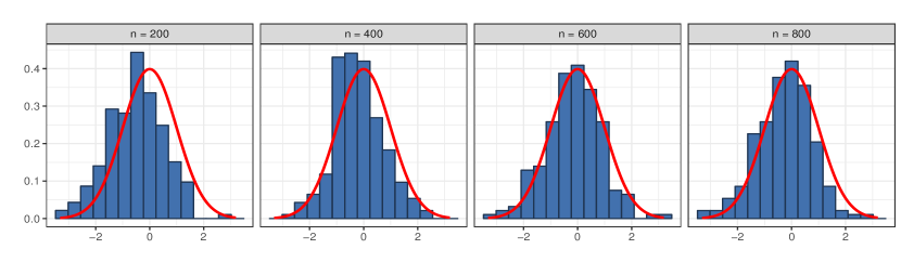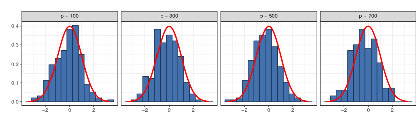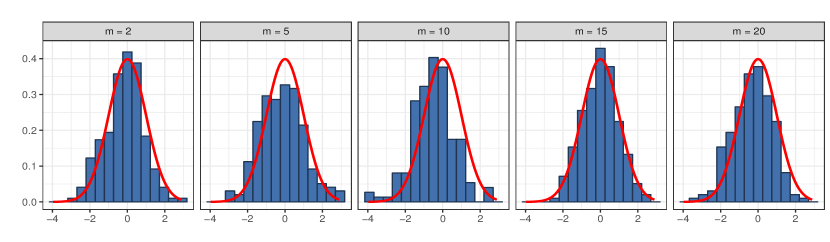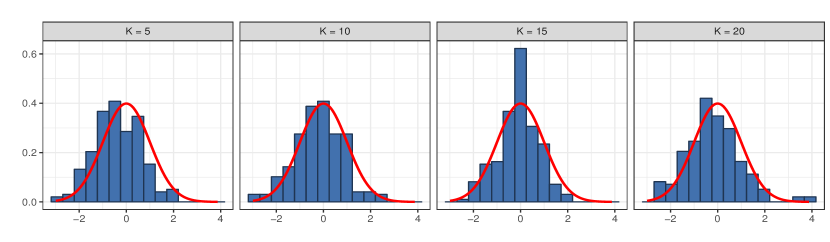Appendix J Additional simulation results: estimation and inference of $\beta$ when the number of latent factors is not consistently estimated

We discuss the impact of selecting $\widehat{K}$ with $\widehat{K}\neq K$ on the estimation and inference of $\beta$, particularizing to the case when some columns of $A$ have very weak signals such that our estimate $\widehat{K}$ is smaller than the true $K$. We start by offering some intuition here. Intuitively, when the submatrix $A_{\cdot S^{c}}$ contains many zero entries for some index set $S\subseteq[K]$, our procedure of estimating $K$ is likely to miss the latent factors in $S^{c}$, but may still recover $Z_{S}$. As a result, only $A_{\cdot S}$ can be well estimated. Consider the simple case $\Sigma_{Z}=\bf{I}_{K}$ and recall that $\beta=(A^{T}A)^{-1}A^{T}\Sigma_{XY}$. Replacing $A$ by $A_{\cdot S}$ yields

$$(A_{\cdot S}^{T}A_{\cdot S})^{-1}A_{\cdot S}^{T}\Sigma_{XY}=(A_{\cdot S}^{T}A_{\cdot S})^{-1}A_{\cdot S}^{T}A\beta=\beta_{S}+\underbrace{(A_{\cdot S}^{T}A_{\cdot S})^{-1}A_{\cdot S}^{T}A_{\cdot S^{c}}\beta_{S^{c}}}_{\Delta}.$$

Therefore, when $A_{\cdot S^{c}}$ is small such that $\Delta$ is small, we still have

$$(A_{\cdot S}^{T}A_{\cdot S})^{-1}A_{\cdot S}^{T}\Sigma_{XY}~{}\approx~{}\beta_{S}.$$

When $\Sigma_{Z}$ is not diagonal, the dependence among the latent factors also affects this approximation.

To empirically investigate the impact of the estimating error of $\widehat{K}$ on the subsequent inferential result, we conduct the following two simulation studies.

(1) We take the same generating mechanism as described in Section 6 and consider $p=400$, $n=300$, $K=10$ and $m=5$. The matrix $\Sigma_{Z}$ is set to be $\sigma_{Z}^{2}\bf{I}_{K}$ with $\sigma_{Z}^{2}=3$. After generating the matrix $A$, we draw an index set from $p$ i.i.d. Bernoulli$(1-\theta)$ with $\theta\in(0,1)$, and manually change the entries $A_{jK}$ into zero, for all $j$ in this index set. The parameter $\theta$ controls the overall sparsity (or signal) of the $K$th column of $A$. Small values of $\theta$ correspond to small signal $A_{\cdot K}$. Note that $A$ no longer necessarily meets our model requirement (A1), since the entries in the $K$th column of $A$ corresponding to pure variables are not necessarily 1, and allowed to be set to zero. We allowed for this misspecification since we empirically found that as long as there exists at least two entries in the $K$th column of $A$ corresponding to pure variables (even though the rest entries of $A_{\cdot K}$ are zero), our algorithm continues to consistently estimate $K$.

Our goal is to verify if the resulting estimator $\widehat{\beta}$ estimates $\beta$ well expect for the $K$th coordinate and to examine the empirical coverage of the 95% confidence intervals of our proposed estimator. The same estimators mentioned in Section 6 of the main paper are considered. For the oracle estimator $\widehat{\beta}_{\rm oracle}$, to illustrate the effect of using a subset of $Z$, we change it to

$$\widehat{\beta}_{\rm oracle}=\left({\bf Z}_{\cdot\widehat{K}}^{T}{\bf Z}_{\cdot\widehat{K}}\right)^{-1}{\bf Z}_{\cdot\widehat{K}}^{T}{\bf Y}$$

where $\widehat{K}$ is estimated from Algorithm 1. We vary $\theta\in\{0.1,0.3,0.5,0.8\}$ and, for each setting, we calculate the averaged mean squared error of the subvector $[\widehat{\beta}-\beta]_{S(1)}$, with $S(1):=\{1,2,\ldots,K-1\}$, for different estimators, as well as the averaged coverage of the 95% confidence intervals for $\beta_{1}$, over 200 repetitions. These results together with the averaged estimated $K$ are reported in Table 4.

Result: When $\theta$ is small, that is, $A_{\cdot K}$ has very weak signal, our procedure of estimating $K$ is likely to miss the $K$th latent factor, leading to $\widehat{K}=9$, as expected. The estimation of the first $K-1$ entries of $\beta$ is only slightly affected. Our proposed estimator $\widehat{\beta}$ has the second best performance, after the oracle estimator. The coverage of the 95% confidence intervals constructed from $\widehat{\beta}$ is slightly under the nominal 95% level. As $\theta$ increases ($\theta\geq 0.5$), that is, the signal of $A_{\cdot K}$ gets larger, we consistently estimate $K$, and consequently, our proposed estimator performs increasingly better in terms of both the estimation error and the coverage of 95% confidence intervals.

(2) We now consider the case when there are multiple, sparse columns of $A$. We take the same setting $p=400$, $n=300$, $K=10$, $m=5$ and $\Sigma_{Z}=\sigma_{Z}^{2}\bf{I}_{K}$ with $\sigma_{Z}^{2}=3$. For each $n_{A}\in\{1,2,\ldots,5\}$, we threshold the last $n_{A}$ columns of $A$ according to the procedure described in the previous paragraph with $\theta=0.1$. For each $n_{A}$, let $S(n_{A})=\{1,2,\ldots,K-n_{A}\}$. The averaged mean squared error of $[\widehat{\beta}-\beta]_{S(n_{A})}$, the averaged coverage of the 95% confidence intervals for $\beta_{1}$ and the averaged estimated $K$ are reported in Table 4.

Result: As expected, the estimated number of factors is smaller than the true value, $10$, and is close to $K-n_{A}$, the number of columns of $A$ that have strong signals. As long as $n_{A}\leq 4$, the estimation of $\beta_{S(n_{A})}$ seems fairly good, and $\widehat{\beta}$ still has the best performance (after $\widehat{\beta}_{\rm oracle}$). The coverage of the 95% confidence intervals constructed from $\widehat{\beta}$ is still close to, though slightly lower than, 95%. As $n_{A}$ increases, more latent factors have weak signals. This makes estimation of $K$ more difficult and clearly affects the estimation of $\beta$ and the coverage of confidence intervals.

(3) We further investigate the effect of the correlation of $Z$ on the impact of inconsistently estimating $K$. We choose $\Sigma_{Z}$ as $[\Sigma_{Z}]_{ij}=\sigma_{Z}^{2}(-1)^{i+j}\rho^{|i-j|}$ for each $i,j\in[K]$ with $\sigma_{Z}^{2}=3$. We vary $\rho\in\{0.1,0.2,0.3,0.4,0.5\}$ and fix $\theta=0.1$, $n_{A}=1$, $p=400$, $n=300$, $K=10$ and $m=5$. The averaged mean squared error of the subvector $[\widehat{\beta}-\beta]_{S(1)}$, the averaged coverage of the 95% confidence intervals for $\beta_{1}$ and the averaged estimated $K$ are reported in Table 4.

Result: The estimation errors of all estimators (including $\widehat{\beta}_{\rm oracle}$) increase as $\rho$ gets larger. $\widehat{\beta}^{(I)}$ turns out to be more robust than $\widehat{\beta}$ in the presence of correlated factors. One possible explanation is that $\widehat{\beta}^{(I)}$ targets $\Sigma_{Z}^{-1}(A_{I\cdot}^{T}A_{I\cdot})^{-1}A_{I\cdot}^{T}\text{Cov}(X_{I},Y)$ which, due to the diagonal structure of $A_{I\cdot}^{T}A_{I\cdot}$, is less affected by a non-diagonal $\Sigma_{Z}$ compared to $\widehat{\beta}$. The coverage of the 95% confidence intervals constructed from both $\widehat{\beta}$ and $\widehat{\beta}^{(I)}$ is close to 95%, and slightly decreases as $\rho$ gets larger.

	$\widehat{\beta}$	$\widehat{\beta}^{(I)}$	$\widehat{\beta}_{\rm naive}$	$\widehat{\beta}^{(A)}$	$\widehat{\beta}_{\rm oracle}$	CIs of $\widehat{\beta}$		CIs of $\widehat{\beta}^{(I)}$		$\widehat{K}$
Vary $\theta$ with $n=300$, $p=400$, $K=10$, $m=5$						coverage	length	coverage	length
$\theta=0.1$	0.07	0.08	0.12	0.08	0.02	0.90	0.84	0.91	0.88	9.1
$\theta=0.3$	0.06	0.06	0.11	0.07	0.03	0.90	0.84	0.92	0.87	9.0
$\theta=0.5$	0.03	0.04	0.10	0.06	0.00	0.93	0.68	0.93	0.72	10.0
$\theta=0.8$	0.03	0.03	0.11	0.06	0.00	0.95	0.64	0.94	0.67	10.0
Vary $n_{A}$ with $n=300$, $p=400$, $K=10$, $m=5$
$n_{A}=1$	0.07	0.07	0.12	0.08	0.02	0.92	0.83	0.92	0.87	9.1
$n_{A}=2$	0.10	0.11	0.13	0.11	0.05	0.91	1.05	0.93	1.09	8.1
$n_{A}=3$	0.12	0.13	0.14	0.13	0.07	0.91	1.14	0.93	1.19	7.1
$n_{A}=4$	0.13	0.15	0.13	0.13	0.07	0.93	1.16	0.93	1.21	6.1
$n_{A}=5$	0.18	0.20	0.18	0.18	0.10	0.89	1.32	0.89	1.37	5.2
Vary $\rho$ with $n=300$, $p=400$, $K=10$, $m=5$
$\rho=0.1$	0.07	0.07	0.16	0.10	0.03	0.94	0.83	0.94	0.87	9.1
$\rho=0.2$	0.11	0.09	0.24	0.16	0.06	0.95	0.83	0.96	0.88	9.0
$\rho=0.3$	0.16	0.13	0.33	0.22	0.09	0.92	0.85	0.94	0.89	9.0
$\rho=0.4$	0.24	0.19	0.46	0.31	0.15	0.92	0.85	0.93	0.91	9.0
$\rho=0.5$	0.34	0.28	0.61	0.42	0.21	0.91	0.87	0.93	0.96	9.0

Table 4: $\ell_{2}$ error of various estimators, the coverage and the averaged length of the 95% CIs of $\beta_{1}$ and the estimated number of latent factors.

References

- Ackerman et al. (2018) Ackerman, M. E., Das, J., Pittala, S., Broge, T., Linde, C., Suscovich, T. J., Brown, E. P., Bradley, T., Natarajan, H., Lin, S., Sassic, J. K., O’Keefe, S., Mehta, N., Goodman, D., Sips, M., Weiner, J. A., Tomaras, G. D., Haynes, B. F., Lauffenburger, D. A., Bailey-Kellogg, C., Roederer, M. and Alter, G. (2018). Route of immunization defines multiple mechanisms of vaccine-mediated protection against siv. Nature Medicine 24 1590–1598.
- Ahn and Horenstein (2013) Ahn, S. C. and Horenstein, A. R. (2013). Eigenvalue ratio test for the number of factors. Econometrica 81 1203–1227.
-
Anderson and Amemiya (1988)
Anderson, T. W. and Amemiya, Y. (1988).
The asymptotic normal distribution of estimators in factor analysis
under general conditions.
Ann. Statist. 16 759–771.
URL https://doi.org/10.1214/aos/1176350834 - Anderson and Rubin (1956) Anderson, T. W. and Rubin, H. (1956). Statistical inference in factor analysis. In Proceedings of the Third Berkeley Symposium on Mathematical Statistics and Probability, Volume 5: Contributions to Econometrics, Industrial Research, and Psychometry. University of California Press, Berkeley, Calif.
- Bai (2003) Bai, J. (2003). Inferential theory for factor models of large dimensions. Econometrica 71 135–171.
Bai and Li (2012)
Bai, J. and Li, K. (2012).
Statistical analysis of factor models of high dimension.
Ann. Statist. 40 436–465.
URL https://doi.org/10.1214/11-AOS966 - Bai and Ng (2002) Bai, J. and Ng, S. (2002). Determining the number of factors in approximate factor models. Econometrica 70 191–221.
- Bai and Ng (2006) Bai, J. and Ng, S. (2006). Confidence intervals for diffusion index forecasts and inference for factor-augmented regressions. Econometrica 74 1133–1150.
- Bai and Ng (2008) Bai, J. and Ng, S. (2008). Forecasting economic time series using targeted predictors. Journal of Econometrics 146 304 – 317. Honoring the research contributions of Charles R. Nelson.
- Bair et al. (2006) Bair, E., Hastie, T., Paul, D. and Tibshirani, R. (2006). Prediction by supervised principal components. Journal of the American Statistical Association 101 119–137.
- Belloni et al. (2017) Belloni, A., Rosenbaum, M. and Tsybakov, A. B. (2017). Linear and conic programming estimators in high dimensional errors-in-variables models. Journal of the Royal Statistical Society: Series B (Statistical Methodology) 79 939–956.
- Bien et al. (2016) Bien, J., Bunea, F. and Xiao, L. (2016). Convex banding of the covariance matrix. Journal of the American Statistical Association 111 834–845.
- Bing et al. (2020) Bing, X., Bunea, F. and Wegkamp, M. (2020). Detecting approximate replicate components of a high-dimensional random vector with latent structure.
- Bing et al. (2019a) Bing, X., Bunea, F., Wegkamp, M. and Strimas-Mackey, S. (2019a). Essential regression.
- Bing et al. (2019b) Bing, X., Bunea, F., Yang, N. and Wegkamp, M. (2019b). Adaptive estimation in structured factor models with applications to overlapping clustering. To appear in the Annals of Statistics .
- Blei and McAuliffe (2007) Blei, D. M. and McAuliffe, J. D. (2007). Supervised topic models. In Proceedings of the 20th International Conference on Neural Information Processing Systems. NIPS’07, Curran Associates Inc., USA.
- Boivin and Ng (2006) Boivin, J. and Ng, S. (2006). Are more data always better for factor analysis? Journal of Econometrics 132 169 – 194. Common Features.
- Bollen (1989) Bollen, K. A. (1989). Structural Equations with Latent Variables. Wiley.
- Bournazos and Ravetch (2017) Bournazos, S. and Ravetch, J. V. (2017). Fc receptor function and the design of vaccination strategies. Immunity 47 224–233.
Bunea et al. (2011)
Bunea, F., She, Y. and Wegkamp, M. H. (2011).
Optimal selection of reduced rank estimators of high-dimensional
matrices.
Ann. Statist. 39 1282–1309.
URL https://doi.org/10.1214/11-AOS876 - Bunea et al. (2020) Bunea, F., Strimas-Mackey, S. and Wegkamp, M. (2020). Interpolation under latent factor regression models.
Bunea and Xiao (2015)
Bunea, F. and Xiao, L. (2015).
On the sample covariance matrix estimator of reduced effective rank
population matrices, with applications to fpca.
Bernoulli 21 1200–1230.
URL https://doi.org/10.3150/14-BEJ602 - Chamberlain and Rothschild (1983) Chamberlain, G. and Rothschild, M. (1983). Arbitrage, factor structure, and mean-variance analysis on large asset markets. Econometrica 51 1281–1304.
- Chandrasekaran et al. (2009) Chandrasekaran, V., Sanghavi, S., Parrilo, P. A. and Willsky, A. S. (2009). Sparse and low-rank matrix decompositions. IFAC Proceedings Volumes 42 1493 – 1498. 15th IFAC Symposium on System Identification.
- Connor and Korajczyk (1986) Connor, G. and Korajczyk, R. (1986). Performance measurement with the arbitrage pricing theory: A new framework for analysis. Journal of Financial Economics 15 373–394.
- Fan et al. (2011) Fan, J., Liao, Y. and Mincheva, M. (2011). High-dimensional covariance matrix estimation in approximate factor models. Ann. Statist. 39 3320–3356.
- Fan et al. (2013) Fan, J., Liao, Y. and Mincheva, M. (2013). Large covariance estimation by thresholding principal orthogonal complements. Journal of the Royal Statistical Society: Series B (Statistical Methodology) 75 603–680.
- Fan et al. (2017) Fan, J., Xue, L. and Yao, J. (2017). Sufficient forecasting using factor models. Journal of Econometrics 201 292 – 306.
Forni et al. (2000)
Forni, M., Hallin, M., Lippi, M. and
Reichlin, L. (2000).
The generalized dynamic-factor model: Identification and estimation.
The Review of Economics and Statistics 82 540–554.
URL http://www.jstor.org/stable/2646650 -
Forni and Reichlin (1996)
Forni, M. and Reichlin, L. (1996).
Dynamic Common Factors in Large Cross-Sections.
Empirical Economics 21 27–42.
URL https://ideas.repec.org/a/spr/empeco/v21y1996i1p27-42.html - Giraud (2015) Giraud, C. (2015). Introduction to High-Dimensional Statistics. Monographs on Statistics and Applied Probability.
- Hahn et al. (2013) Hahn, P. R., Carvalho, C. M. and Mukherjee, S. (2013). Partial factor modeling: Predictor-dependent shrinkage for linear regression. Journal of the American Statistical Association 108 999–1008.
Ibragimov and Sharakhmetov (1998)
Ibragimov, R. and Sharakhmetov, S. (1998).
Short communications: On an exact constant for the rosenthal
inequality.
Theory of Probability & Its Applications 42
294–302.
URL https://doi.org/10.1137/S0040585X97976155 -
Joreskog (1970a)
Joreskog, K. G. (1970a).
A general method for analysis of covariance structures.
Biometrika 57 239–251.
URL http://www.jstor.org/stable/2334833 -
Joreskog (1970b)
Joreskog, K. G. (1970b).
A general method for estimating a linear structural equation system*.
ETS Research Bulletin Series 1970 i–41.
URL https://onlinelibrary.wiley.com/doi/abs/10.1002/j.2333-8504.1970.tb00783.x - Kelly and Pruitt (2015) Kelly, B. and Pruitt, S. (2015). The three-pass regression filter: A new approach to forecasting using many predictors. Journal of Econometrics 186 294 – 316. High Dimensional Problems in Econometrics.
- Klopp et al. (2017) Klopp, O., Lu, Y., Tsybakov, A. B. and Zhou, H. H. (2017). Structured Matrix Estimation and Completion. ArXiv e-prints .
- Koopmans and Reiersol (1950) Koopmans, T. C. and Reiersol, O. (1950). The identification of structural characteristics. Ann. Math. Statist. 21 165–181.
- Lawley (1940) Lawley, D. N. (1940). Vi.—the estimation of factor loadings by the method of maximum likelihood. Proceedings of the Royal Society of Edinburgh 60 64–82.
- Lawley and Maxwell (1971) Lawley, D. N. and Maxwell, A. E. (1971). Factor analysis as a statistical method. 2nd ed. American Elsevier Publishing Co., Inc., New York.
- McDonald (1999) McDonald, R. P. (1999). Test theory: a unified treatment. Taylor and Francis.
- Nimmerjahn and Ravetch (2007) Nimmerjahn, F. and Ravetch, J. V. (2007). Fc receptors as regulators of immunity. vol. 96 of Advances in Immunology. Academic Press, 179 – 204.
Onatski (2009)
Onatski, A. (2009).
Testing hypotheses about the number of factors in large factor
models.
Econometrica 77 1447–1479.
URL https://onlinelibrary.wiley.com/doi/abs/10.3982/ECTA6964 - Reiß and Wahl (2016) Reiß, M. and Wahl, M. (2016). Non-asymptotic upper bounds for the reconstruction error of pca.
Rudelson and Vershynin (2010)
Rudelson, M. and Vershynin, R. (2010).
Non-asymptotic Theory of Random Matrices: Extreme Singular
Values.
1576–1602.
URL https://www.worldscientific.com/doi/abs/10.1142/9789814324359_0111 -
Shorack (2017)
Shorack, G. R. (2017).
Probability for Statisticians.
Springer International Publishing, Cham, 23–38.
URL https://doi.org/10.1007/978-3-319-52207-4_2 - Stock and Watson (2002a) Stock, J. H. and Watson, M. W. (2002a). Forecasting using principal components from a large number of predictors. Journal of the American Statistical Association 97 1167–1179.
- Stock and Watson (2002b) Stock, J. H. and Watson, M. W. (2002b). Macroeconomic forecasting using diffusion indexes. Journal of Business & Economic Statistics 20 147–162.
- Thurstone (1931) Thurstone, L. (1931). Multiple factor analysis. Psychological Review 38 406–427.
- Tsybakov (2009) Tsybakov, A. B. (2009). Introduction to nonparametric estimation. Springer Series in Statistics. Springer, New York.
- Vershynin (2012) Vershynin, R. (2012). Introduction to the non-asymptotic analysis of random matrices. Cambridge University Press, 210 – 268.
- Wainwright (2019) Wainwright, M. J. (2019). High-Dimensional Statistics: A Non-Asymptotic Viewpoint. Cambridge Series in Statistical and Probabilistic Mathematics, Cambridge University Press.
Wegkamp and Zhao (2016)
Wegkamp, M. and Zhao, Y. (2016).
Adaptive estimation of the copula correlation matrix for
semiparametric elliptical copulas.
Bernoulli 22 1184–1226.
URL https://doi.org/10.3150/14-BEJ690 -
Yalcin and Amemiya (2001)
Yalcin, I. and Amemiya, Y. (2001).
Nonlinear factor analysis as a statistical method.
Statist. Sci. 16 275–294.
URL https://doi.org/10.1214/ss/1009213729
Appendix A The identifiability of when is known
We state and prove the identifiability of when is known under Assumption 1 but when (A1) is replaced by