Learning Representations by Humans, for Humans

Abstract

When machine predictors can achieve higher performance than the human decision-makers they support, improving the performance of human decision-makers is often conflated with improving machine accuracy. Here we propose a framework to directly support human decision-making, in which the role of machines is to reframe problems rather than to prescribe actions through prediction. Inspired by the success of representation learning in improving performance of machine predictors, our framework learns human-facing representations optimized for human performance. This “Mind Composed with Machine” framework incorporates a human decision-making model directly into the representation learning paradigm and is trained with a novel human-in-the-loop training procedure. We empirically demonstrate the successful application of the framework to various tasks and representational forms.

1 Introduction

“No one ever made a decision because of a number.
  They need a story.”

— Daniel Kahneman

Advancements in machine learning algorithms, as well as increased data availability and computational power, have led to the rise of predictive machines that outperform human experts in controlled experiments (Esteva et al., 2017; Nickerson & Rogers, 2014; Tabibian et al., 2019). However, human involvement remains important in many domains, (Liu et al., 2019), especially those in which safety and equity are important considerations (Parikh et al., 2019; Barabas et al., 2017) and where users have external information or want to exercise agency and use their own judgment. In these settings, humans are the final arbiters, and the goal of algorithms is to produce useful decision aids.

Given that learning algorithms excel at prediction, previous efforts in this space have largely focused on providing predictions as decision aids. This has led to a large body of work on how to make predictions accessible to decision makers, whether through models that are interpretable (Lakkaraju et al., 2016), or through explainable machine learning, in which machine outputs (and so human inputs) are assumed to be predictions and are augmented with explanations (Ribeiro et al., 2016; Lundberg & Lee, 2017). We see two main drawbacks to these approaches. First, setting the role of machines to ‘predict, then explain’ reduces humans to auditors of the ‘expert’ machines (Lai & Tan, 2018). With loss of agency, people are reluctant to adopt predictions and even inclined to go against them (Bandura, 1989, 2010; Yeomans et al., 2017; Dietvorst et al., 2016; Yin et al., 2019; Green & Chen, 2019b). This leads to a degradation in performance of the human-machine pipeline over time (Elmalech et al., 2015; Dietvorst et al., 2015; Logg, 2017; Stevenson & Doleac, 2018). More importantly, these methods cannot adapt to the ways in which predictions are used, and so are unable to adjust for systematic human errors or to make use of human capabilities.

Moving beyond predictions, in this paper we advocate for broader forms of learnable advice and capitalize on a different strength of machine learning: the ability to learn useful representations. Inspired by the success of representation learning, in which deep neural networks learn data representations that enable ‘simple’ (i.e., linear) predictors to perform well (Bengio et al., 2013), we leverage neural architectures to learn representations that best support human decision-makers (Kahneman, 2011; Miller, 1956). Consider a multi-layered neural network ${\mathcal{N}}=f\circ{\phi}$ composed of a high-dimensional representation mapping ${\phi}$ and a predictor $f$. Our key proposal is to remove the predictor and instead plug the human decision function $h$ into the learning framework to obtain $h\circ{\phi}$, allowing us to optimize the representation mapping to directly improve human performance.

Our framework for optimizing $h\circ{\phi}$, which we refer to as ‘Mind Composed with Machine’ (M$\circ$M) contributes to work that seeks to bridge machine learning with human-centric design (Sutton et al., 2020; Venkatesh et al., 2003), and we make two key contributions in this regard. First, rather than machines that predict or decide, we train models that learn how to reframe problems for a human decision-maker. We learn to map problem instances to representational objects such as plots, summaries, or avatars, aiming to capture problem structure and preserve user autonomy. This approach of “advising through reframing” draws on work in the social sciences that shows that the quality of human decisions depends on how problems are presented (Thompson, 1980; Cosmides & Tooby, 1992; Gigerenzer & Hoffrage, 1995; Kahneman & Tversky, 2013; Brown et al., 2013). Second, rather than optimizing for machine performance, we directly optimize for human performance. We learn representations of inputs for which human decision-makers perform well rather than those under which machines achieve high accuracy. In this, we view our approach as taking a step towards promoting machine learning as a tool for human-intelligence augmentation (Licklider, 1960; Engelbart, 1962).

The immediate difficulty in learning human-facing representations in M$\circ$M is that $h$ encodes how actual human decision-makers respond to representational advice and so is not amenable to differentiation (we cannot “backprop through $h$.”) To overcome this, we propose an iterative human-in-the-loop procedure that alternates between (i) learning a differentiable surrogate model of human decision-making at the current representation, and (ii) training the machine model end-to-end using the current surrogate. For estimating the surrogate model we query actual humans for their decisions given a current representation.

We demonstrate the M$\circ$M framework on three distinct tasks, designed with two goals in mind: to explore different forms of human-facing representations and to highlight different benefits that come from the framework. The first experiment focuses on classifying point clouds in a controlled environment. Here we show how the M$\circ$M framework can learn scatter-plot representations that allow for high human accuracy without explicitly presenting machine-generated predictions (or decisions). The second experiment considers loan approvals and adopts facial avatars as the form of representational advice. Here we demonstrate that the framework can be applied at scale (we train using $\sim$ 5,000 queries to Amazon mTurk) and also explore what representations learn to encode and how these representations are used to support human decision-making. The third experiment is designed to demonstrate the capacity of our framework to support decision-making in ways that outperform either human or machine alone. Here we use a simulated environment to show how M$\circ$M can learn a representation that enables a human decision-maker to incorporate side-information (consider e.g. a hospital setting, in which doctors have the option to run additional tests or query the patient for information not included in the machine model), even when this information is known only to the user.

On the use of facial avatars: In our study on loan approval we convey advice through a facial avatar that represents an algorithmic assistant. We take care to ensure that users understand this, and understand that the avatar does not represent a loan applicant. We also restrict the avatar to carefully chosen variations on the image of a single actor. We are interested to experiment with facial avatars as representations because facial avatars are high dimensional, abstract (i.e., not an object that is in the domain studied), and naturally accessible to people. We are aware of the legitimate concerns regarding the use of faces in AI systems and the potential for discrimination (West & Crawford, 2019) and any use of facial representations in consequential decision settings must be done with similar care.

2 Related Work

2.1 Modeling Human Factors

Recent studies have shown that the connections between trust, accuracy, and explainability can be complex and nuanced. Human users tend to use algorithmic recommendations less frequently than would be beneficial  (Green & Chen, 2019a; Lai & Tan, 2018), and user trust (as measured by agreement with algorithmic recommendation) does not increase proportionately to model accuracy (Yin et al., 2019). Increasing model interpretability may not increase trust (as measured by agreement with the model), and may decrease users’ ability to identify model errors (Poursabzi-Sangdeh et al., 2018). Further, even when explanations increase acceptance of model recommendations, they do not increase self-reported user trust or willingness to use the model in the future (Cramer et al., 2008). In fact, explanations increase acceptance of model recommendations even when they are nonsensical (Lai & Tan, 2019) or support incorrect predictions (Bansal et al., 2020). At the same time, understanding human interactions with machine learning systems is crucial; for example, whether or not users retain agency has been shown to affect users’ acceptance of model predictions (Dietvorst et al., 2016), providing support for our approach. Recent work acknowledges that human decision processes must be considered when developing decision support technology (Lai et al., 2020; Bansal et al., 2019), and work in cognitive science has shown settings in which accurate models of human decision-making can be developed (Bourgin et al., 2019).

2.2 Humans in the Loop

Despite much recent interest in training with “humans in the loop,” experimentation in this setting remains an exceptionally challenging task. The field of interactive machine learning has successfully used human queries to improve machine performance in tasks where human preferences determine the gold standard (Amershi et al., 2014), but human-in-the-loop training has been less productive in adapting predictive machines to better accommodate human decision-makers. In the field of interpretable machine learning, optimization for human usage generally relies on proxy metrics of human interpretability in combination with machine accuracy (Lage et al., 2019), with people only used to evaluate performance at test time. A few exceptions have allowed human feedback to guide model selection among similarly-accurate machine-optimized models (Ross et al., 2017; Lage et al., 2018), incorporating human preferences. In regard to using human responses as part of a feedback loop to a learning system, we are only aware of Lage et al. (2018), and the authors actually abandoned attempts to train with mTurkers.

2.3 Collaboration with Machine Arbiters

A related field considers learning when a machine learning system should defer to a human user instead of making a prediction. This setting, unlike ours, allows the machine to bypass a human decision-maker  (Madras et al., 2018; Mozannar & Sontag, 2020; Wilder et al., 2020). In this setting, human accuracy is considered to be fixed and independent of the machine learning system, and in evaluation human decisions are either fully simulated or based on previously gathered datasets.

3 Method

Figure 1: Left: The M$\circ$M framework. The neural network learns a mapping ${\phi}$ from inputs $x$ to representations $z$, such that when $z$ is visualized through ${\rho}$, representations elicit good human decisions. Right: Training alternates between (A) querying users for decisions on the current representations, (B) using these to train a human surrogate network ${\hat{h}}$, and (C) re-training representations.

In a typical setting, a decision-making user is given an instance $x\in{\cal{X}}$. For clarity, consider ${\cal{X}}={\mathbb{R}}^{d}$. Given $x$, the user must decide on an action ${a}\in{{\cal{A}}}$. For example, if $x$ are details of a loan application, then users can choose ${a}\in\{\texttt{approve},\texttt{deny}\}$. Each instance is also associated with a ground-truth outcome $y\in{\cal{Y}}$, so that $(x,y)$ is sampled from an unknown distribution $D$. We assume that users seek to choose actions that minimize an incurred loss ${\ell}(y,{a})$, with ${\ell}$ also known to the system designer; e.g., for loans, $y$ denotes whether a loan will be repaid. We consider the general class of prediction policy problems (Kleinberg et al., 2015), where the loss function is known and the difficulty in decision-making is governed by how well $y$ can be predicted.

We denote by $h$ the human mapping from inputs to decisions or actions. For example, ${a}=h(x)$ denotes a decision based on raw instances $x$. Other sources of input such as explanations $e$ or representations can be considered; e.g., ${a}=h(x,{\hat{y}},e)$ denotes a decision based on $x$ together with prediction ${\hat{y}}$ and explanation $e$. We allow $h$ to be either deterministic or randomized, and conceptualize $h$ as either representing a particular target user or a stable distribution over different kinds of users. We assume the mapping $h$ is fixed (if there is adaptation to a representation, then $h$ can be thought of as the end-point of this adaptation).

Crucially, we also allow machines to present users with machine-generated advice ${\gamma}(x)$, with human actions denoted as ${a}=h({\gamma}(x))$. Users may additionally have access to side information $s$ that is unavailable to the machine, in which case user actions are ${a}=h({\gamma}(x),s)$. Advice ${\gamma}(x)$ allows for a human-centric representation of the input, and we seek to learn a mapping ${\gamma}$ from inputs to representations under which humans will make good decisions. The benchmark for evaluation is the expected loss of human actions given this advice:

$$\mathbb{E}_{D}{[{{\ell}(y,{a})}]},\qquad\mbox{for}\quad{a}=h({\gamma}(x)).$$ (1)

3.1 Predictive Advice

A standard approach provides human users with machine-generated predictions, ${\hat{y}}=f(x)$, where $f$ is optimized for predictive accuracy and there is a straightforward mapping from predictions to prescribed actions $\hat{y}\rightarrow\hat{y}_{a}$ (e.g., for some known threshold, ‘probability of returning loan’ corresponds to ‘approve loan’). This is a special case of our framework where advice ${\gamma}=(x,{\hat{y}})$, and the user is modeled as $a={\hat{y}}_{a}=h(x,{\hat{y}})$. The predictive model is trained to minimize:

$$\min\nolimits_{f}\mathbb{E}_{D}{[{{\ell}(y,{\hat{y}}_{a})}]},\qquad\mbox{for}\quad{\hat{y}}=f(x).$$ (2)

In this approach, predictions $f(x)$ are useful only to the extent that they are followed. Moreover, predictions provide only a scalar summary of the information in $x$, and limit the degree to which users can exercise their cognitive and decision-making capabilities; e.g., in the context of side information.

3.2 Representational Advice

In M$\circ$M, we allow advice ${\gamma}$ to map inputs into representations that are designed to usefully convey information to a human decision-maker (e.g., a scatterplot, a compact linear model, or an avatar). Given a representation class ${\Gamma}$ we seek a mapping ${\gamma}\in{\Gamma}$ that minimizes expected loss $\min_{{\gamma}\in{\Gamma}}\mathbb{E}_{D}{[{{\ell}(y,h({\gamma}(x)))}]}$. With a training set ${\mathcal{S}}=\{(x_{i},y_{i})\}_{i=1}^{m}$ sampled from distribution $D$, and with knowledge of the human mapping $h$, we would seek ${\gamma}$ to minimize the empirical loss:

$$\min_{{\gamma}\in{\Gamma}}\sum_{i=1}^{m}{\ell}(y_{i},{a}_{i}),\qquad\mbox{for}\quad{a}_{i}=h({\gamma}(x_{i})),$$ (3)

possibly under some form of regularization (more details below). Here, ${\Gamma}$ needs to be rich enough to contain flexible mappings from inputs to representations while also generating objects that are accessible to humans. To achieve this, we decompose algorithmic advice ${\gamma}(x)={\rho}({\phi}_{\theta}(x))$ into two components:

$\bullet$ ${\phi}_{\theta}:{\mathbb{R}}^{d}\rightarrow{\mathbb{R}}^{k}$ is a parameterized embedding model with learnable parameters ${\theta}\in{\Theta}$, that maps inputs into vector representations $z={\phi}_{\theta}(x)\in{\mathbb{R}}^{k}$ for some $k>1$, and

$\bullet$ ${\rho}:{\mathbb{R}}^{k}\rightarrow{\mathcal{V}}$ is a visualization component that maps each $z$ into a visual object ${v}={\rho}(z)\in{\mathcal{V}}$ (e.g., a scatterplot, a facial avatar).

This decomposition is useful because for a given application of M$\circ$M we can now fix the visualization component ${\rho}$, and seek to learn the embedding component ${\phi}_{\theta}$. This process of learning a suitable embedding through feedback from human users, is what we mean by “learning representations by humans [from feedback], for humans.” Henceforth, it is convenient to fold the visualization component ${\rho}$ into the human mapping $h$, and write $h(z)$ to mean $h({\rho}(z))$, for embedding $z={\phi}_{\theta}(x)$. The training problem (3) becomes:

$$\min_{{\theta}\in{\Theta}}\sum_{i=1}^{m}{\ell}(y_{i},{a}_{i}),\quad\mbox{for}\ {a}_{i}=h({\phi}_{\theta}(x_{i})),$$ (4)

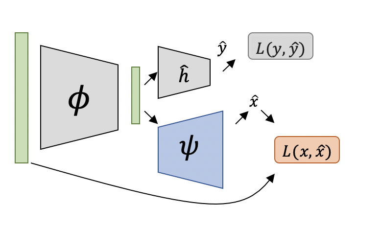
again, perhaps with some regularization. By solving (4), we learn representations that promote good decisions by the human user. See Figure 1 (left).

Regularization.

Regularization may play a number of different roles: as with typical L2 regularization, it may be used to reduce overfitting of the representation network, encouraging representations that generalize better to new data points. It may also be used to encourage some desired property such as sparsity, which may be beneficial for many visualizations, given the limited ability of human subjects to process many variables simultaneously. Regularization can also be used in our framework to encode domain knowledge regarding desired properties of representations, for example when the ideal representation has a known mathematical property. We utilize this form of regularization in Experiments 1 and 2.

Choosing Appropriate Visualizations.

Determining the form of representational advice that best-serves expert decision-makers in any concrete task will likely require in-depth domain knowledge and should be done with care. The characterization of varying visualizations’ effects on decision-making is sufficiently elaborate as to warrant its own field of study (Lurie & Mason, 2007), and thus we focus here on learning to adapt a particular choice of representation from within a set of “approved” representational forms.

3.3 Training Procedure, and Human Proxy

We adopt a neural network to model the parameterized embedding ${\phi}_{\theta}(x)$, and thus advice ${\gamma}$. The main difficulty in optimizing (4) is that human actions $\{{a}_{i}\}_{i=1}^{m}$ depend on ${\phi}_{\theta}(x)$ via an unknown $h$ and yet gradients of ${\theta}$ must pass through $h$. To handle this, we make use of a differentiable surrogate for $h$, denoted ${\hat{h}}_{\eta}:{\mathbb{R}}^{k}\rightarrow{\Gamma}$ with parameters ${\eta}\in{H}$. We learn this surrogate, referring to it as “h-hat.”

The M$\circ$M human-in-the-loop training procedure alternates between two steps:

1. Use the current ${\theta}$ to gather samples of human decisions ${a}=h(z)$ on inputs $z={\phi}_{\theta}(x)$ and fit ${\hat{h}}_{\eta}$.

2. Find ${\theta}$ to optimize the performance of ${\hat{h}}_{\eta}\circ{\phi}_{\theta}$ for the current ${\eta}$, as in (4).

Figure 1 (right) illustrates this process; for pseudocode see Appendix A). Since ${\hat{h}}$ is trained to be accurate for the current embedding distribution rather than globally, ${\hat{h}}$ is unlikely to exactly match $h$. However, for learning to improve, it suffices for ${\hat{h}}$ to induce parameter gradients that improve loss (see Figure 7 in the Appendix). Still, ${\hat{h}}$ must be periodically retrained because as parameters ${\theta}$ change, so does the induced distribution of representations $z$ (and ${\hat{h}}_{\eta}$ may become less accurate).

Initialization of ${\theta}$.

In some applications, it may be useful to initialize ${\phi}$ using a machine-only model with architecture equal to ${\hat{h}}({\phi})$. In applications in which the human must attend to the same features as the machine model, this can help to focus ${\phi}$ on those features and minimize exploration of representations that do not contain decision-relevant information. This can be particularly useful when the representation lies within the domain of the data (e.g. plots, subsets).

When a desired initial distribution of representations is known, ${\phi}$ can be positioned as the generator of a Wasserstein GAN (Arjovsky et al., 2017). In this case, the labels are not used at all, and thus the initial mapping is used only to achieve a certain coverage over the representation space and not expected to encode feature information from a machine-only model.

3.4 Handling Side Information

One way humans could surpass machines is through access to side information ${s}$ that is informative of outcome $y$ yet unknown to the machine. The M$\circ$M framework can be extended to learn a representation ${\gamma}(x)$ that is optimal conditioned on the existence of ${s}$, despite the machine having no access to ${s}$. At test time, the human has access to ${s}$, and so action ${a}=h({\phi}(x),s)$. The observation is that the ground-truth outcome $y$, which is available during training, conveys information about $s$: if ${s}$ is informative of $y$, then there exist $x$ for which the outcome $y$ varies with ${s}$. Thus $(x,y)$ is jointly informative of ${s}$: for such $x$, knowing $y$ and modeling the mechanism $y=g_{x}(s)$ by which ${s}$ affects $y$ for a given $x$ would allow reverse-engineering the value of ${s}$ as $g_{x}^{-1}(y)$. Although ${s}$ cannot generally be exactly reconstructed without supervision on ${s}$ (e.g. due to inexact modeling or non-invertibility of $g_{x}$), in some cases $(x,y)$ can be used to make useful inference about ${s}$. Intuitively, note that for a given $x$, multiple $y\in\{y_{1}\ldots y_{k}\}$ values correspond to multiple $s$ values. If $h$ varies with $s$, without access to $s$ or $y$, the best ${\hat{h}}(x)$ we can learn is $\mathbb{E}_{s\sim S}{[{h(x,s)}]}$. With varied $y_{i}$ which correspond to different values of $s$, we can learn ${\hat{h}}(x,y_{i})=\mathbb{E}_{s\sim S|y=y_{i}}{[{h(x,s)}]}$ for each $y_{i}$, which allow ${\hat{h}}$ to incorporate information about $s$.

4 Experimental Results

We report the results of three distinct experiments. Our intent is to demonstrate the breadth of the framework’s potential, and the experiments we present vary in the task, the form of advice, their complexity and scale, and the degree of human involvement (one experiment is simulated, another uses thousands of mTurk queries). We defer some of the experimental details to the Appendix.

Model Selection

Experimenting with humans in-the-loop is expensive and time-consuming, making standard practices for model selection such as cross-validation difficult to carry out. This necessitates committing to a certain model architecture at an early stage and after only minimal trail-and-error. In our experiments, we rely on testing architectures in a machine-only setting with various input and output distributions to ensure sufficient flexibility to reproduce a variety of potential mappings, as well as limited human testing with responses from the authors. Our model choices produced favorable results with minimal tuning. We believe this suggests some useful robustness of the approach to model selection choices, but future work would be beneficial to better understand sensitivity to model selection.

4.1 Decision-compatible Scatterplots

In the first experiment, we focus on learning useful, low-dimensional representations of high-dimensional data, in the form of scatterplots. To make high-dimensional data more accessible to users, it is common practice to project into a low-dimensional embedded space and reason based on a visualization, for example a scatter plot or histogram. The choice of how to project high-dimensional data into a lower-dimensional space is consequential to decision-making (Kiselev et al., 2019), and yet standard dimensionality-reduction methods optimize statistical criteria (e.g., maximizing directional variation in PCA) rather than optimizing for success in user interpretation. The M$\circ$M framework learns projections that, once visualized, directly support good decisions.

We consider a setting where the goal is to correctly classify objects in $p$-dimensional space, $p>2$. Each $x$ is a $p$-dimensional point cloud consisting of $m=40$ points in ${\mathbb{R}}^{p}$ (so $x\in{\mathbb{R}}^{40p}$). Point clouds are constructed such that, when orthogonally projected onto a particular linear 2D subspace of ${\mathbb{R}}^{p}$, denoted $V$, they form the shape of either an ‘X’ or an ‘O’, this determining their true label $y$. All directions orthogonal to $V$ contain similarly scaled random noise. In the experiment, we generate 1,000 examples of these point clouds in 3D.

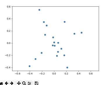
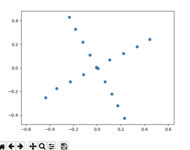
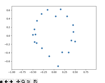
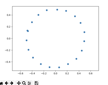
Subjects are presented with a series of scatterplots, which visualize the point clouds for a given 2D projection, and are asked to determine for each point cloud its label (‘X’ or ’O’). Whereas a projection onto $V$ produces a useful representation, most others do not, including those learned from PCA. Our goal is to show that M$\circ$M can use human feedback to learn a projection (${\phi}$) that produces visually meaningful scatterplots (${\rho}$), leading to good decisions.

Model.

Here, representation ${\phi}$ plays the role of a dimensionality reduction mapping. We use $d=3$ and set ${\phi}$ to be a 3x2 linear mapping with parameters ${\theta}$ as a 3x2 matrix. This is augmented with an orthogonality penalty ${\phi}^{T}{\phi}-\mathbb{I}$ to encourage matrices which represent rotations. For the human proxy model, we want to be able to roughly model the visual perception of subjects. For this, we use for $\hat{h}$ a small, single-layer 3x3 convolutional network, that takes as inputs a differentiable 6x6 histogram over the 2D projections.

Figure 2: 2D representations of point clouds. (A) Points in their original 3D representation give little visual indication of class (X or O). (B) Shapes become easily distinguishable when projected onto an appropriate subspace (shown in bold). (Bottom) Learned 2D representations after each training round (‘X’, ‘O’ are overlaid). The initial 2D projection (round 1), on which a machine-classifier is fully accurate, is unintelligible to people. However, as training progresses, feedback improves the projection until the class becomes visually apparent (round 4), with very high human accuracy.

Results.

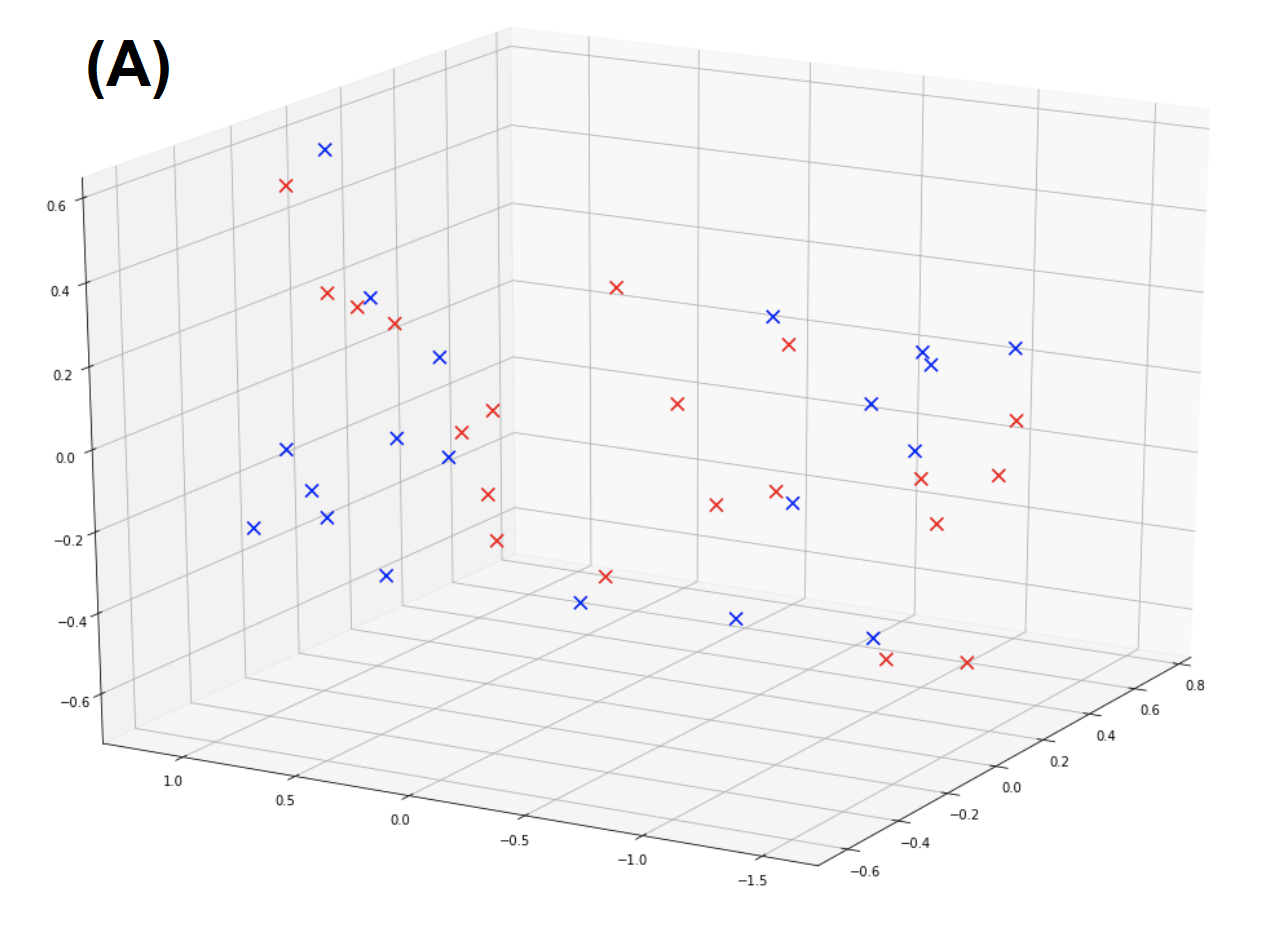
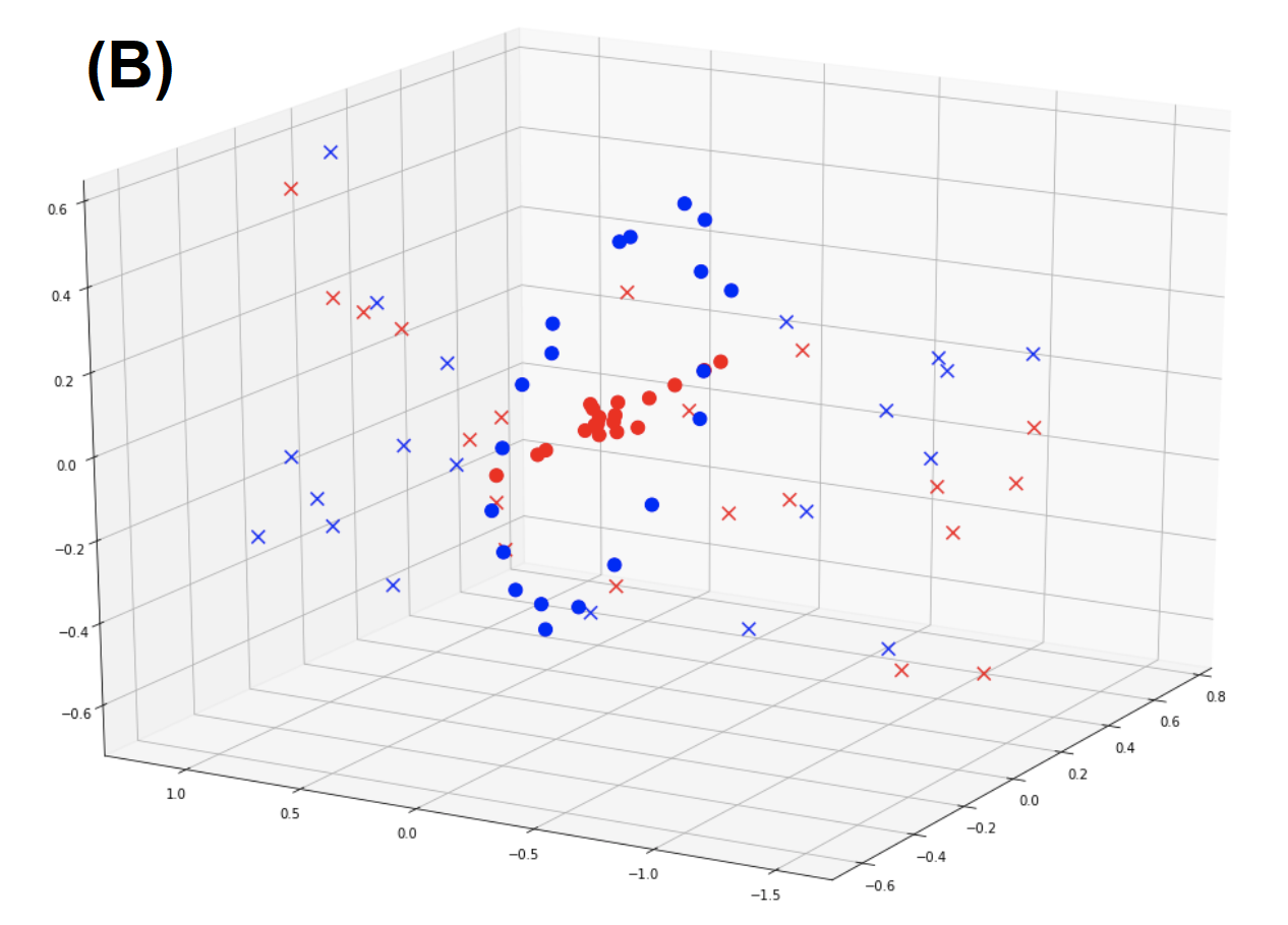
We recruited 12 computer science students to test the M$\circ$M framework. Participants watched an instructional video and then completed a training and testing phase, each having five rounds (with intermittent model optimization) of 15 queries to label plots as either ‘X’ or ‘O’. The results we provide refer to the testing phase. Round 1 includes representations based on a random initialization of model parameters and therefore serves as a baseline condition. The results show that participants achieve an average accuracy of 68% in round 1, but improve to an average accuracy of 91% in round 5, a significant improvement of 23% ($p<.01$, paired $t$-test) with 75% of participants achieving 100% accuracy by round 5. Subjects are never given machine-generated predictions or feedback, and improvement from training round 1 to testing round 1 is negligible (3%), suggesting that progress is driven solely by the successful reframing of problem instances (not humans getting better at the task).

Figure 2 demonstrates a typical example of a five-round sequential training progression. Initially, representations produced by M$\circ$M are difficult to classify when ${\theta}$ is initialized arbitrarily. (This is also true when ${\theta}$ is initialized with a fully accurate machine-only model.) As training progresses, feedback regarding subject perception gradually rotates the projection, revealing distinct class shapes. Training progress is made as long as subject responses carry some machine-discernible signal regarding the subject’s propensity to label a plot as ‘X’ or ‘O’. M$\circ$M utilizes these signals to update the representations and improve human performance.

Figure 3: Different facial avatars, each avatar representing an algorithmic assistant and not a loan applicant, and trained to provide useful advice through facial expressions. The leftmost avatar is set to a neutral expression ($z=0$).

4.2 Decision-compatible Algorithmic Avatars

For this experiment we consider a real decision task and use real data (approving loans), train with many humans participants (mTurkers), and explore a novel form of representational advice (facial avatars). Altogether we elicit around 5,000 human decisions for training and evaluation. Specifically we use the Lending Club dataset, focusing on the resolved loans, i.e., loans that were paid in full ($y=1$) or defaulted ($y=0$), and only using features that would have been available to lenders at loan inception. The decision task is to determine whether to approve a loan (${a}=1$) or not (${a}=0$), and the loss function we use is ${\ell}(y,a)=\mathds{1}_{\{{y\neq a}\}}$.

Goals, Expectations, and Limitations.

Whereas professional decision-makers are inclined to exercise their own judgment and deviate from machine advice (Stevenson & Doleac, 2019; De-Arteaga et al., 2020), mTurkers are non-experts and are likely to follow machine predictions (Lai & Tan, 2019; Yin et al., 2019). For this reason, the goal of the experiment is not to demonstrate performance superiority over purely predictive advice, nor to show that mTurkers can become expert loan officers. Rather, the goal is to show that abstract representations can convey predictive advice in a way that requires users to deliberate, and to explore whether humans use learned representations differently than they use machine predictions in making decisions. In Appendix B we further discuss unique challenges encountered when training with mTurkers in the loop.

Figure 4: Human accuracy in the algorithmic advice condition (‘avatar advice’) consistently increases over rounds. Performance quickly surpasses the ‘no advice’ (data only) condition, and steadily approaches performance of users observing algorithmic predictions (‘predictive advice’), which in itself is lower than machine-only performance (‘machine accuracy’). Human accuracy falls when faces are shuffled within predicted labels of $\hat{h}$, confirming that faces convey useful, multi-variate information.

Representations.

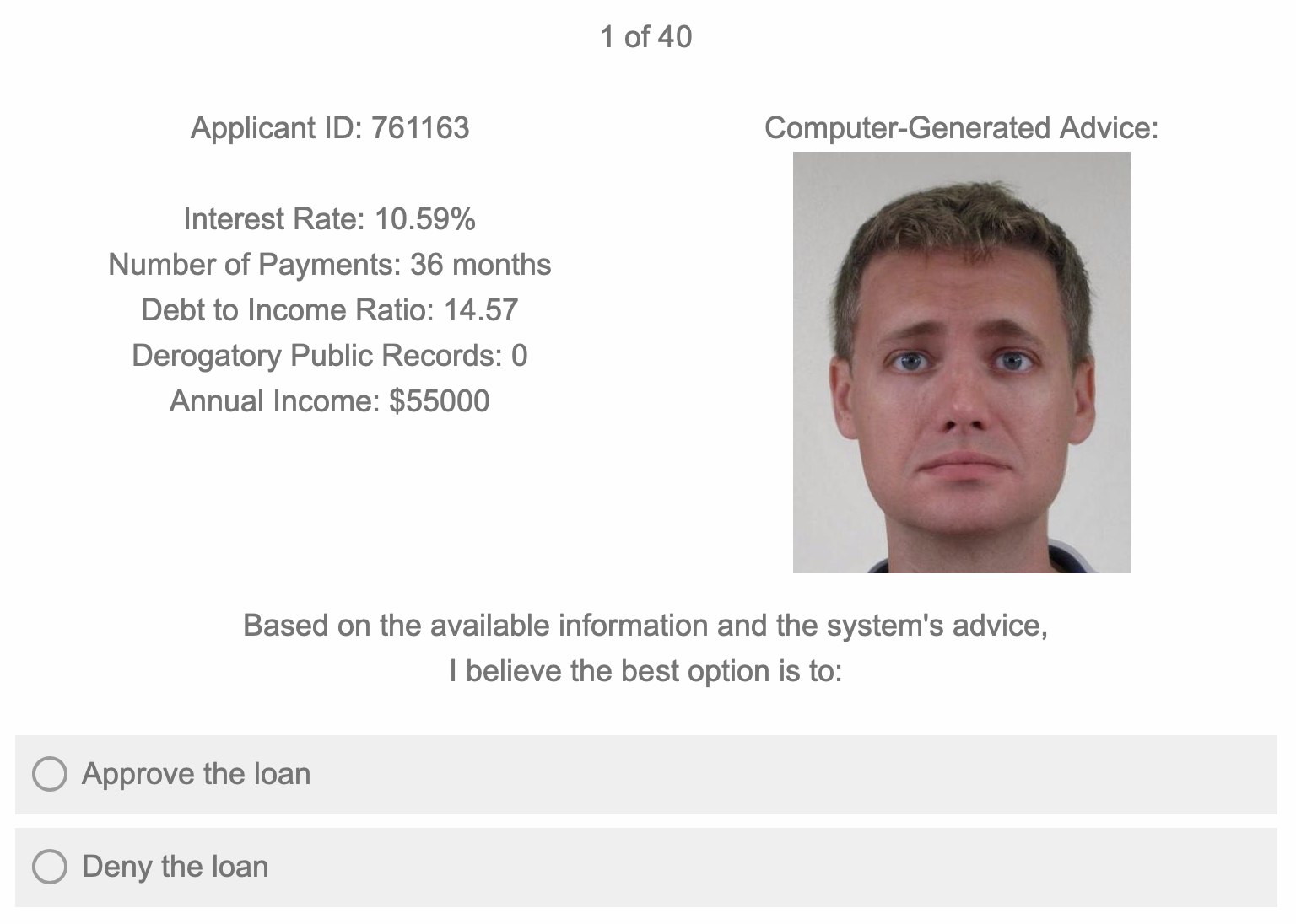
With the aim of exploring broader forms of representational advice, we make use of a facial avatar, framed to users as an algorithmic assistant— not the recipient of the loan —and communicating through its facial expressions information that is relevant to a loan decision. The avatar is based on a single, realistic-looking face capable of conveying versatile expressions (Figure 4 includes some examples). Expressions vary along ten dimensions including basic emotions (Du et al., 2014), social dimensions (e.g., dominance and trustworthiness (Du et al., 2014; Todorov et al., 2008)), and subtle changes in appearance (e.g., eye gaze). Expressions are encoded by the representation vector $z$, with each entry corresponding to a different facial dimension. Thus, vectors $z$ can be thought of as points in $k$-dimensional ‘face-space’ in which expressions vary smoothly with $z$.

We are interested in facial avatars because they are abstract (i.e., not in the domain of the input objects) and because they have previously been validated as useful representations of information (Chernoff, 1973; Lott & Durbridge, 1990). They are also high-dimensional representations, and non-linear in the input features; that is, faces are known to be processed holistically with dependencies beyond the sum of their parts (Richler et al., 2009). Faces also leverage innate human cognition—immediate, effortless, and fairly consistent processing of facial signals (Izard, 1994; Todorov et al., 2008; Freeman & Johnson, 2016).

Through M$\circ$M, we learn a mapping from inputs to avatars that is useful for decision-making. Training is driven completely by human responses, and learned expressions reflect usage patterns that users found to be useful, as opposed to hand-coded mappings as in Chernoff faces (Chernoff, 1973).

Model and Training.

We set ${\phi}$ to be a small, fully connected network with a single 25-hidden unit layer, mapping inputs to representation vectors $z\in{\mathbb{R}}^{9}$. The visualization component ${\rho}(z)$ creates avatars by morphing a set of base images, each corresponding to a facial dimension, with $z$ used to weight the importance of each base image. For regularization, we additionally consider the loss of a decoder network implemented by an additional neural network, which attempts to reconstruct the input $x$ from the representation. This term encourages points in face-space to preserve distances in instance-space at the cost of some reduction in accuracy. This promotes representations that carry more information about inputs than that implied by simple predictions. For ${\hat{h}}$ we use a small, fully connected network with two layers of size 20 each, operating directly on representation vectors $z$.

In collecting human decisions for training ${\hat{h}}$, mTurkers were queried for their decisions regarding the approval or denial of loan applications. New users were recruited at each round to obtain reports that are as independent as possible and to control for any human learning. Each user was queried for a random subset of 40 training examples, with the number of users chosen to ensure that each example would receive multiple responses (w.h.p.). For predictive purposes, binary outputs were set to be the majority human response. Each loan application was presented using the most informative features as well as the avatar. We did not relate to users any specific way in which they should use avatar advice, and care was taken to ensure users understood that the avatar does not itself represent an applicant. Appendix C.2 provides additional experimental details.

Results.

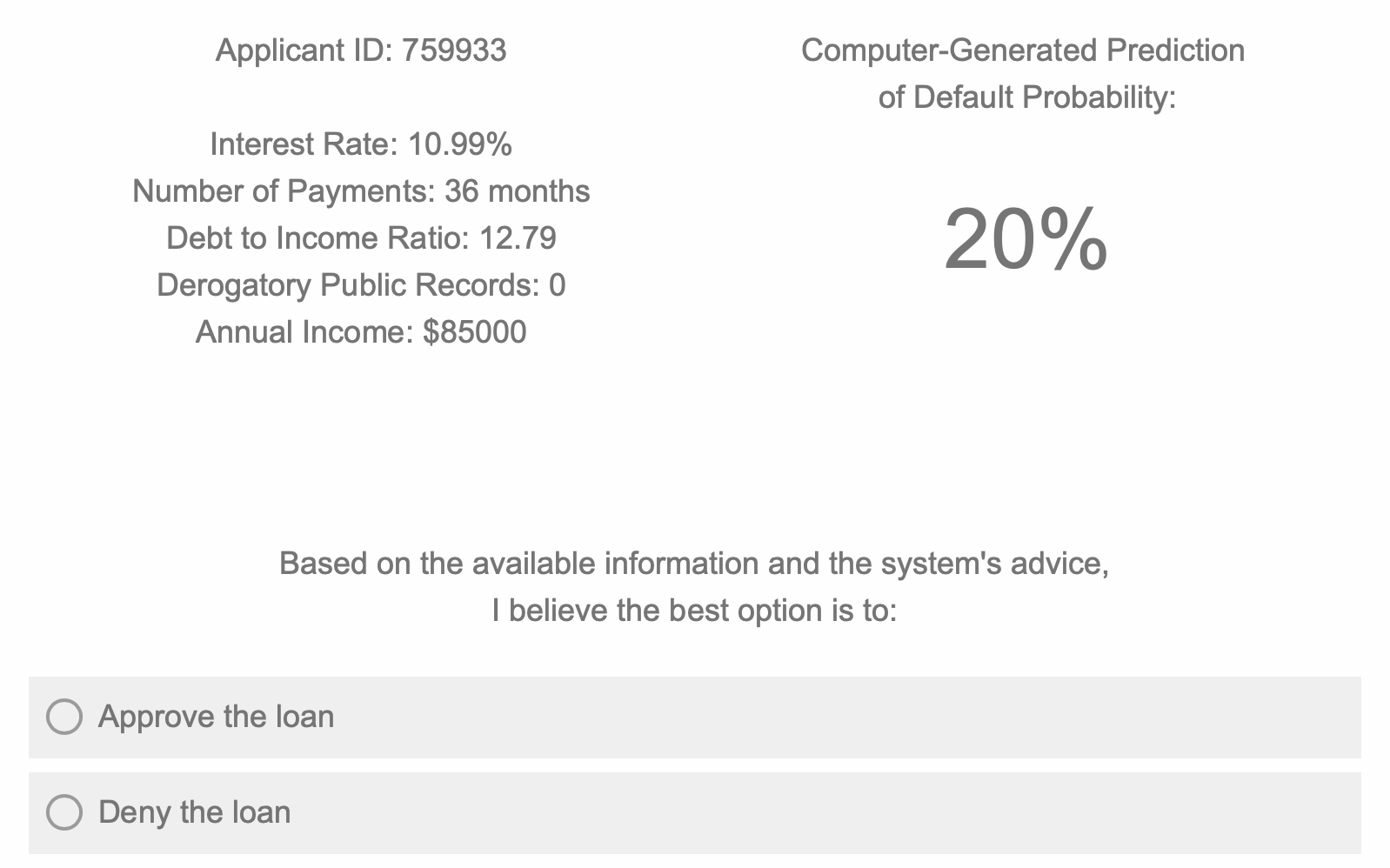
Our results show that M$\circ$M can learn representations that support good decisions through a complex, abstract representation, and that this representation carries multivariate information, making it qualitatively different than prediction. As benchmarks, we consider the accuracy of a trained neural network model ${\mathcal{N}}(x)$ having architecture equal to ${\hat{h}}\circ{\phi}$ (but otherwise unrelated to our human experiments), as well as human performance under predictive advice ${\gamma}(x)={{\tilde{y}}}\in[0,1]$ where ${{\tilde{y}}}$ is the predicted probability of ${\mathcal{N}}(x)$. We also consider a condition with ‘shuffled’ avatar advice, which we describe below.

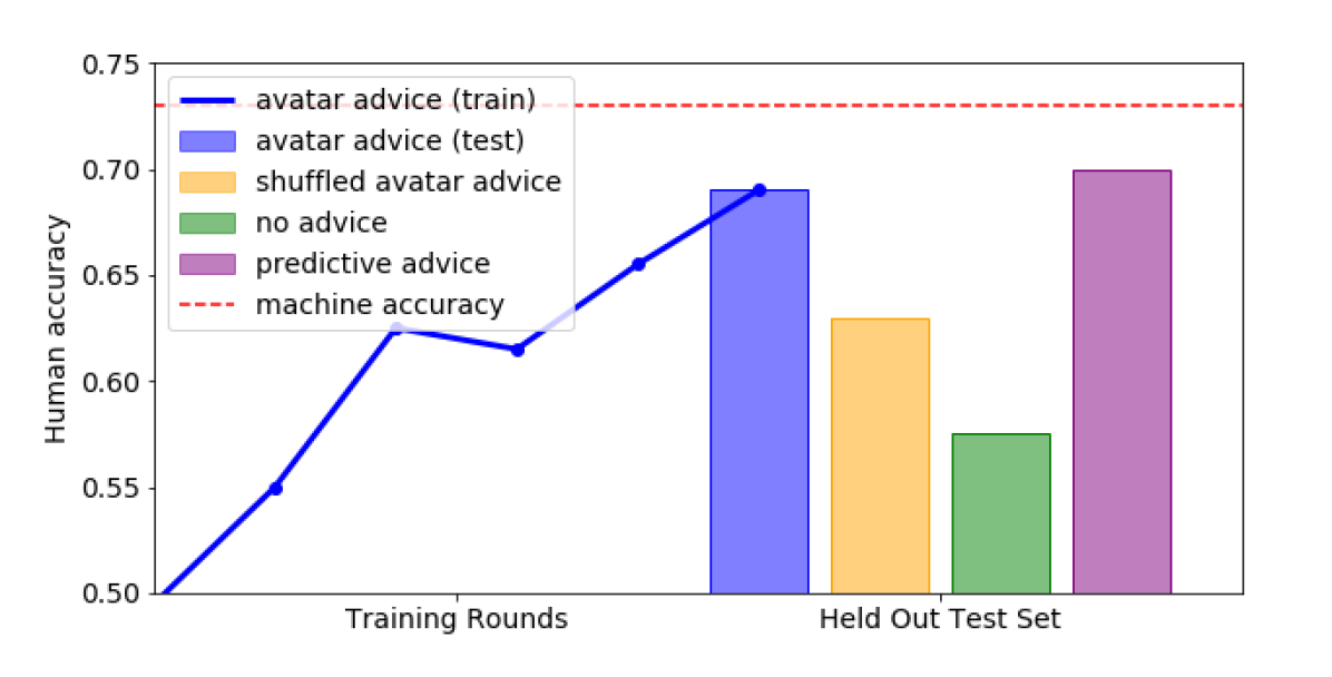
Figure 4 shows the training process and resulting test accuracy (data is balanced so chance$\,\,\approx 0.5$). At first, the (randomly-initialized) representation ${\phi}$ produces arbitrary avatars, and performance in the avatar condition is lower than in the no-advice condition. This indicates that users take into account the (initially uninformative) algorithmic advice. As learning progresses, user feedback accumulates and the accuracy from using the M$\circ$M framework steadily rises. After six rounds, avatar advice contributes to a boost of 11.5% in accuracy (0.69) over the no-advice condition (0.575), reaching 99% of the accuracy in the predictive advice condition (0.70). Performance in the predictive advice condition does not reach machine accuracy (0.73), showing that not all subjects follow predictive advice.

Analysis.

We additionally explore what the representations learn, and how humans incorporate them into predictions. One possible concern is that despite regularization, learned avatars may simply convey stylized binary predictions (e.g., happy or sad faces). To explore this, we added a ‘shuffled’ condition in which faces are shuffled within predicted labels of ${\hat{h}}$. As shown in Figure 4, shuffling degrades performance, confirming that faces convey more information than the system’s binary prediction. Moreover, the avatars do not encode a univariate (but not binary) prediction, and humans do not use the information in the same way that they use numeric predictions: (i) no single feature of $z$ has a correlation with predicted human responses ${\hat{h}}(z)$ of more than $R^{2}=0.7$, (ii) correlations of average human response with features $z$ are low ($R^{2}\leq 0.36$ across features) while responses in the predictive condition have $R^{2}=0.73$ with the predictions, and (iii) users in the avatar condition self-report using the data as much or more than the advice 83% of the time, compared to 47% for the predictive advice condition.

At the same time, $z$ preserves important information regarding $x$. To show this, we train linear models to predict from $z$ each of the data features: interest rate (rate), loan term (term), debt to income ratio (dti), negative public records (rec), annual income (inc), employment length (emp). Results show that $z$ is highly informative of rate ($R^{2}=0.79$) and term ($0.57$), mildly informative of rec ($-0.21$), inc ($0.23$), and emp ($0.13$), and has virtually no predictive power of dti ($-0.03$). Further inspecting model coefficients reveals a complex pattern of how $z$ carries information regarding $x$ (see Appendix C.2.4 for all coefficients). E.g.: trustworthiness plays an important part in predicting all features, whereas anger is virtually unused; happiness and sadness do not play opposite roles—happiness is significant in term, while sadness is significant in rate; and whereas emp is linked almost exclusively to age variation, inc is expressed by over half of the facial dimensions.

4.3 Incorporating Side Information

To demonstrate additional capabilities of M$\circ$M  we show that the framework can also learn representations that allow a decision maker to leverage side information that is unavailable to the machine. Access to side information is one advantage humans may have over machines, and our goal here is to show the potential of representations in eliciting decisions whose quality surpasses that attainable by machines alone. We adopt simulation for this experiment because it is challenging for non-experts (like mTurkers) to outperform purely predictive advice, even with access to additional side information. Simulation also allows us to systematically vary the synthetic human model, and we consider four distinct models of decision-making.

We consider a medical decision-making task in which doctors must evaluate the health risk of incoming ER patients and have access to a predictive model. Here, we focus on compact, linear models, and view the model coefficients along with the input features as the representation, affecting the decision process of doctors. Doctors additionally have access to side information that is unavailable to the model and may affect their decision. Our goal is to learn a model that can account for how doctors use this side information.

Setup.

There are four primary binary features $x\in\{0,1\}^{4}$: diabetes ($x_{d}$), cardiovascular disease ($x_{c}$), race ($x_{r}$), and income level ($x_{i}$). An integer ‘side-information’ variable ${s}\in\{0,1,2,3\}$ encodes how long the patient’s condition was allowed to progress before coming to the ER and is available only to the doctor. We assume ground-truth risk $y$ is determined only by diabetes, cardiovascular disease, and time to ER, through $y=x_{d}+x_{c}+{s}$, where $x_{d},x_{c},{s}$ are sampled independently. We also assume that $x_{r},x_{i}$ jointly correlate with $y$ (e.g. due to disparities in access), albeit not perfectly, so that they carry some but not all signal in ${s}$, whereas $x_{d},x_{c}$ do not; see Appendix C.3.1 for full details). In this way, $x_{r}$ and $x_{i}$ offer predictive power beyond that implied by their correlations with known health conditions ($x_{d}$, $x_{c}$), but interfere with use of side information.

We model a decision maker who generally follows predictive advice ${\hat{y}}=f_{w}(x)=\langle{w,x}\rangle$, but with the capacity to adjust the machine-generated risk scores at her discretion and in a way that depends on the model through its coefficients $w$. We assume that doctors are broadly aware of the correlation structure of the problem, and are prone to incorporate the available side information ${s}$ into ${\hat{y}}$ if they believe this will give a better risk estimate. We model the decisions of a population of doctors as incorporating ${s}$ additively and with probability that decreases with the magnitude of either of the coefficients $w_{r}$ or $w_{i}$. We refer to this as the or model and set $h_{\text{or}}(x,{s},w)={\hat{y}}+I(w)\cdotp{s}$ with $I(w)\propto 1/(\max\{w_{r},w_{i}\})$. We also consider simpler decision models: always using side information ($h_{\text{always}}$), never using side information ($h_{\text{never}}$), and a coarse variant of $h_{\text{or}}$ using binarized side information, $h_{\text{coarse}}={\hat{y}}+I(w)\cdotp 2\cdotp\mathds{1}{\{{{s}\geq 2}\}}$.

Model.

The representation ${\rho}(z)$ consists of $x$, coefficients $w$ (these are learned within ${\phi}$), and ${\hat{y}}=\langle{w,x}\rangle$. The difficulty in optimizing ${\phi}$ is that ${s}$ is never observed, and our proposed solution is to use $y$ (which is known at train time) as a proxy for ${s}$ when fitting ${\hat{h}}$, which is then used to train ${\phi}$ (see Section 3). Since $x$ and $y$ jointly carry information regarding ${s}$, we define ${\hat{h}}(x,y;w)=\langle{w,x}\rangle+{\hat{{s}}}(x,y)$, where ${\hat{{s}}}(x,y)=v_{0}y+\sum_{j=1}^{4}v_{j}x_{j}$, and $v$ are parameters. Note that it is enough that ${\hat{{s}}}$ models how the user utilizes side information, rather than the value of $s$ directly; $s$ is never observed, and there is no guarantee about the relation between ${\hat{{s}}}$ and ${s}$.

	M$\circ$M	$h(\text{{Machine}})$
Or	1.0	.894
Coarse Or	.951	.891
Never	.891	.891
Always	1.0	.674

Table 1: Performance of M$\circ$M with side information on four synthetic human models. Machine-only performance is 0.890.

Results.

We compare M$\circ$M to two other baselines: a machine-only linear regression, and the human model $h$ applied to this machine-only model, and evaluate performance on the four synthetic human models ($h_{\text{or}},h_{\text{coarse}},h_{\text{never}}$, and $h_{\text{always}}$). Both M$\circ$M and the baselines use a linear model but the model in M$\circ$M is trained to take into account how users incorporate side information. For evaluation, we consider binarized labels $y_{bin}=\mathds{1}{\{{y>3}\}}$.

We report results averaged over ten random data samples of size 1,000 with an 80-20 train-test split. As Table 1 shows, due to its flexibility in finding a representation that allows for incorporation of side information by the user, M$\circ$M reaches 100% accuracy for the or and always decision models. M$\circ$M maintains its advantage under the coarse-or decision model (i.e., when doctors use imperfect information), and remains effective in settings where side information is never used. The problem with the baseline model is that it includes non-zero coefficients for all four features. This promotes accuracy in a machine-only setting, and in the absence of side information. Given this, the or and coarse-or decision models only very rarely introduce the side information— and this is indeed the best they can do given that the machine model uses all four variables. In contrast, for the always decision model the user always introduces side information, causing over-counting of the time to ER effect on patient outcomes (because of correlations between ${s}$ and $x_{r}$ and $x_{i}$). In contrast, M$\circ$M learns a linear model that is responsive to the human decision-maker: for example, including non-zero coefficients for only $x_{d}$ and $x_{c}$ with the or decision model.

5 Discussion

We have introduced a novel learning framework for supporting human decision-making. Rather than view algorithms as experts, asked to explain their conclusions to people, we position algorithms as advisors whose goal is to help humans make better decisions while retaining human agency. The M$\circ$M framework learns to provide representations of inputs that provide advice and promote good decisions. We see this as a promising direction for promoting synergies between learning systems and people and hope that by tapping into innate cognitive human strengths, learned representations can improve human-machine collaboration by prioritizing information, highlighting alternatives, and correcting biases.

Our hope is that centering humans in the decision process will lead to augmenting intelligence but also facilitate transparency. Unfortunately, this may not always be the case, and ethical, legal, and societal aspects of systems that are optimized to promote particular human decisions must be subject to scrutiny by both researchers and practitioners.

We believe algorithmic decision support, when thoughtfully deployed, exhibits great potential. Systems designed specifically to provide users with the information and framing they need to make good decisions can harness the strengths of both computer pattern recognition and human judgment and information synthesis. We can hope that the combination of mind and machine can do better than either alone. The ideas presented in this paper serve as a step toward this goal.

We advocate for responsible and transparent deployment of models with “h-hat-like” components, in which system goals and user goals are aligned, and humans are aware of what information they provide about their thought processes. Opportunities and dangers of our framework generally reflect those of the broader field of persuasive technology, and ethical guidelines developed in that community should be carefully considered (Fogg, 1998; Berdichevsky & Neuenschwander, 1999).

Appendix A Optimization Algorithm

Algorithm 1 Alternating optimization algorithm

1:  Initialize $\theta=\theta_{0}$

2:  repeat

3:     $x_{1},\dots,x_{n}\sim{\mathcal{S}}$ {Sample $n$ train examples}

4:     $z_{i}\leftarrow\phi_{\theta}(x_{i})\,\,\,\forall\,i\in[n]$ {Generate representations}

5:     ${a}_{i}\leftarrow h({\rho}(z_{i}))\,\,\,\forall\,i\in[n]$ {Query human decisions}

6:     ${\mathcal{T}}=\{(z_{i},{a}_{i})\}_{i=1}^{n}$

7:     ${\eta}\leftarrow\operatorname*{argmin}_{{\eta}^{\prime}}\mathbb{E}_{{\mathcal{T}}}{[{{\ell}({a},{\hat{h}}_{{\eta}^{\prime}}(z))}]}$ {Train ${\hat{h}}$}

8:     $\theta\leftarrow\operatorname*{argmin}_{\theta^{\prime}}\mathbb{E}_{{\mathcal{S}}}{[{{\ell}(y,{\hat{h}}_{\eta}({\phi}_{{\theta}^{\prime}}(x)))}]}$ {Train ${\phi}$}

9:  until convergence

Appendix B General Optimization Issues

B.1 Initialization

Because acquiring human labels is expensive, it is important to initialize ${\phi}$ to map to a region of the representation space in which there is variation and consistency in human reports, such that gradients lead to progress in subsequent rounds.

In some representation spaces, such as our 2D projections of noisy 3D rotated images, this is likely to be the case (almost any 3D slice will retain some signal from the original 2D image). However, in 4+ dimensions, as well as with the subset selection and avatar tasks, there are no such guarantees.

To minimize non-informative queries, we adopt two initialization strategies:

1. Initialization with a computer-only model: In scenarios in which the representation space is a (possibly discrete) subset of input space, such as in subset selection, the initialization problem is to isolate the region of the input space that is important for decision-making. In this situation, it can be useful to initialize with a computer-only classifier. This classifier should share a representation-learning architecture with ${\phi}$ but can have any other classifying architecture appended (although simpler is likely better for this purpose). This should result in some ${\phi}$ which at least focuses on the features relevant for classification, if not necessarily in a human-interpretable format.

2. Initialization to a desired distribution with a WGAN: In scenarios in which the initialization problem is to isolate a region of representation space into which to map all inputs, as in the avatar example, in which we wish to test a variety of expressions without creating expression combinations which will appear overly strange to participants, it can be useful to hand-design a starting distribution over representation space and initialize ${\phi}$ with a Wasserstein GAN (Arjovsky et al., 2017). In this case, we use a Generator Network with the same architecture as ${\phi}$ but allow the Discriminator Network to be of any effective architecture. As with the previous example, this results in an ${\phi}$ in which the desired distribution is presented to users, but not necessarily in a way that reflects any human intuitive concept.

B.2 Convergence

As is true in general of gradient descent algorithms, the M$\circ$M framework is not guaranteed to find a global optimum but rather is likely to end up at a local optimum dependent on both the initialization of ${\phi}$ and $\hat{h}$. In our case, however, the path of gradient descent is also dependent on the inherently stochastic selection and behavior of human users. If users are inconsistent or user groups at different iterations are not drawn from the same behavior distribution, it is possible that learning at one step of the algorithm could result in convergence to a suboptimal distribution for future users. It remains for future work to test how robust machine learning methods might be adapted to this situation to mitigate this issue.

(a) Initial

(b) Step 3 ‘x’

(c) Step 4 ‘x’

(d) Step 3 ‘o’

(e) Step 4 ‘o’

Figure 5: Images of x-o interface

B.3 Regularization/Early Stopping

As mentioned in Section 3, training ${\phi}$ will in general shift the distribution of the representation space away from the region on which we have collected labels for $\hat{h}$ in the previous iterations, resulting in increasing uncertainty in the predicted outcomes. We test a variety of methods to account for this, but developing a consistent scheme for choosing how best to maximize the information in human labels remains future work.

• Regularization of $\hat{h}$: We test regularization of $\hat{h}$ both with Dropout and L2 regularization, both of which help in preventing overfitting, especially in early stages of training, when the representation distribution is not yet refined. As training progresses and the distribution ${\phi}_{\theta}(x)$ becomes more tightly defined, decreasing these regularization parameters increases performance.

• Training $\hat{h}$ with samples from previous iterations: We also found it helpful in early training iterations to reuse samples from the previous human labeling round in training $\hat{h}$, as inspired by [Bobu et al. 2018]. We weight these samples equally and use only the previous round, but it may be reasonable in other applications to alter the weighting scheme and number of rounds used.

• Early stopping based on Bayesian Linear Regression: In an attempt to quantify how the prediction uncertainly changes as ${\theta}$ changes, we also implement Bayesian Linear Regression, found in [Riquelme et al., 2018] to be a simple but effective measure of uncertainty, over the last layer of $\hat{h}({\phi}_{\theta})$ as we vary ${\theta}$ through training. We find that in early iterations of training, this can be an effective stopping criterion for training of ${\phi}$. Again, as training progresses, we find that this mostly indicates only small changes in model uncertainty.

B.4 Human Input

Testing on mTurk presents various challenges for testing the M$\circ$M framework:

• In some applications, such as loan approval, mTurk users are not experts. This makes it difficult to convince them that anything is at stake (we found that bonuses did not meaningfully affect performance). It is also difficult to directly measure effort, agency, trust, or autonomy, all of which result in higher variance in responses.

• In many other applications, the ground truth is generated by humans to begin with (for example, sentiment analysis). Since we require ground truth for training, in these task it cannot be expected of humans to outperform machines.

• As the researchers found in (Lage et al., 2018), there can be a large variance in the time users take to complete a given task. Researchers have found that around 25% of mTurk users complete several tasks at once or take breaks during HITs [Moss and Litman, 2019]. making it difficult to determine how closely Turkers are paying attention to a given task. We use requirements of HIT approval rate greater than 98%, US only, and at least 5,000 HITs approved, as well as a simple comprehension check.

• Turker populations can vary over time and within time periods, again leading to highly variable responses, which can considerably effect the performance of learning.

• Recently, there have been concerns regarding the usage of automated bots within the mTurk communiy. Towards this end, we incorporated in the experimental survey a required reading comprehension task and as well as a CAPTCHA task, and filtered users that did not succeed in these.

Appendix C Experimental Details

C.1 Decision-compatible 2D projections

In the experiment, we generate 1,000 examples of these point clouds in 3D. The class of ${\phi}$ is a 3x3 linear layer with no bias, where we add a penalization term on ${\phi}^{T}{\phi}-\mathbb{I}$ during training to constrain the matrix to be orthogonal. Humans are shown the result of passing the points through this layer and projecting onto the first two dimensions. The class of $\hat{h}$ is a small network with 1 3x3 convolutional layer creating 3 channels, 2x2 max pooling, and a sigmoid over a final linear layer. The input to this network is a soft (differentiable) 6x6 histogram over the 2D projection shown to the human user.

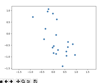
We tested an interactive command line query and response game on 12 computer science students recruited on Slack and email. Users filled out a consent form online, watched an instructional video, and then completed a training and testing round, each with up to 5 rounds of 15 responses. Due to the nature of the training process, achieving 100% accuracy results in ${\phi}$ not updating in the following round. With this in mind, if a user reached 100% accuracy in training, they immediately progressed to testing. If a user reached 100% accuracy in testing, the program exited. ${\phi}$ was able to find a representation that allowed for 100% accuracy 75% of the time, with an average 5 round improvement of 23% across all participants. Many times the resulting projection appeared to be an ‘x’ and ‘o’, as in Figure 5, but occasionally it was user-specific. For example, a user who associates straight lines with the ‘x’ may train the network to learn any projection for ‘x’ that includes many points along a straight line.

The architecture of ${\phi}$ and $\hat{h}$ are described in Section 4. For training, we use a fixed number of epochs (500 for $\hat{h}$ and 300 for ${\phi}$) with base learning rates of .07 and .03, respectively, that increase with lower accuracy scores and decrease with each iteration. We have found these parameters to work well in practice, but observed that results were not sensitive to their selection. The interface allows the number of rounds and examples to be determined by the user, but often 100% accuracy can be achieved after about 5 rounds of 15 examples each.

C.2 Decision-compatible algorithmic avatars

C.2.1 Data Preprocessing.

We use the Lending Club dataset, which we filter to include only loans for which we know the resolution (either default or paid in full, not loans currently in progress) and to remove all features that would not have been available at funding time. We additionally drop loans that were paid off in a single lump sum payment of at least 5 times the normal installment. This results in a dataset that is 49% defaulted and 51% repaid loans. Categorical features are transformed to one-hot variables. There are roughly 95,000 examples remaining in this dataset, of which we split 20% into the test set.

Figure 6: Visualization of reconstruction component

C.2.2 Learning architecture and pipeline.

The network ${\phi}$ takes as input the standardized loan data. Although the number of output dimension are ${\mathbb{R}}^{9}$, ${\phi}$ outputs vectors in ${\mathbb{R}}^{11}$. This is because the some facial expressions do not naturally coexist as compound emotions, i.e., happiness and sadness [Du et al., 2014]. Hence, we must add some additional constraints to the output space, encoded in the extra dimensions. For example, happiness and sadness are split into two separate parameters (rather than using one dimension with positive for happiness and negative for sadness). The same is true of “happy surprise”, which is only allowed to coincide with happiness, as opposed to “sad surprise.” For parameters which have positive and negative versions, we use a tanh function as the final nonlinearity, and for parameters which are positive only, we use a sigmoid function as the final nonlinearity.

These parameters are programmatically mapped to a series of Webmorph (DeBruine & Tiddeman, 2016) transformation text files, which are manually loaded into the batch transform/batch edit functions of Webmorph. We use base emotion images from the CFEE database [Du et al., 2014] and trait identities from [Oosterhof and Todorov, 2008]. This forms ${\rho}$ for this experiment.

The network ${\phi}$ is initialized with a WGAN to match a distribution of parameters chosen to output a fairly uniform distribution of feasible faces. To achieve this, each parameter was chosen to be distributed according to one of the following: a clipped $\mathcal{N}(0,4)$, $\mathcal{U}[0,1]$, or Beta(1,2). The choice of distribution was based on inspection as to what would give reasonable coverage over the set of emotional representations we were interested in testing. In this initial version of ${\phi}$, $x$ values end up mapped randomly to representations, as the WGAN has no objective other than distribution matching.

(a) Loss in training $\hat{h}$ over 3 rounds

(b) Validation Accuracy in training ${\phi}$ over 3 rounds

Figure 7: $\hat{h}$ does not necessarily have to match $h$ well to lead to an increase in accuracy

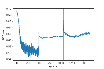
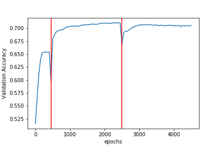
The hidden layer sizes of ${\phi}$ and ${\hat{h}}$ were chosen via cross validation. For ${\phi}$, we use the smallest architecture out of those tested capable of recreating a wide distribution of representations $z$ as the generator of the WGAN. For ${\hat{h}}$, we use the smallest architecture out of those tested that achieves low error both in the computer-only simulation and with the first round of human responses.

In the first experiment, we collect approximately 5 labels each (with minor variation due to a few mTurk users dropping out mid-experiment) for the LASSO feature subset of 400 training set $x$ points and their ${\phi}_{0}$ mappings (see Figure 9). $a$ is taken to be the percentage of users responding “approve” for each point.

(a) Training Rounds (‘Overall‘ here is average per user score, rather than the score of the average response per question)

(b) Test Round

Figure 8: Results by Reported User Type

(a)

(b)

Figure 9: Images from mTurk questionnaire

To train $\hat{h}$, we generate 15 different training-test splits of the collected $\{z,a\}$ pairs and compare the performance of variations of $\hat{h}$ in which it is either initialized randomly or with the $\hat{h}$ from the previous iteration, trained with or without adding the samples from the previous iteration, and ranging over different regularization parameters. We choose the training parameters and number of training epochs which result in the lowest average error across the 15 random splits. In the case of random initialization, we choose the best out of 30 random seeds over the 15 splits.

To train ${\phi}$, we fix $\hat{h}$ and use batches of 30,000 samples per epoch from the training set, which has 75,933 examples in total. To prevent mode collapse, wherein faces “binarize” to two prototypical exemplars, we add a reconstruction regularization term ${R}(x)=\|x-{\psi}({\phi}(x))\|_{2}^{2}$ to the binary cross entropy accuracy loss, where ${\psi}$ is a decoder implemented by an additional neural network (see Figure 6). ${\phi}$ here also features a constraint penalty that prevents co-occurrence of incompatible emotions.

We train ${\phi}$ for 2,000 epochs with the Adam optimizer for a variety of values of $\alpha$, where we use $\alpha$ to balance reconstruction and accuracy loss in the form $\mathcal{L}_{total}=\alpha\mathcal{L}_{acc}+(1-\alpha)\mathcal{L}_{rec}$. We choose the value of $\alpha$ per round that optimally retains $x$ information while promoting accuracy by inspecting the accuracy vs. reconstruction MSE curve. We then perform Bayesian Linear Regression over the final layer of the current $\hat{h}$ for every 50th epoch of ${\phi}$ training and select the number of epochs to use by the minimum of either 2,000 epochs or the epoch at which accuracy uncertainty has doubled. In all but the first step, this resulted in using 2,000 epochs. At each of the 2-5th epochs, we choose only 200 training points to query. In the 6th epoch we use 200 points from the test set.

C.2.3 Self-reported user type.

In the end of the survey, we ask users to report their decision method from among the following choices:

• I primarily relied on the data available

• I used the available data unless I had a strong feeling about the advice of the computer system

• I used both the available data and the advice of the computer system equally

• I used the advice of the computer system unless I had a strong feeling about the available data

• I primarily relied on the advice of the computer system

• Other

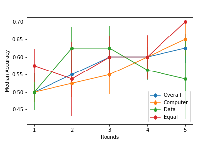
The percentage of users in each of these groups varied widely from round to round.

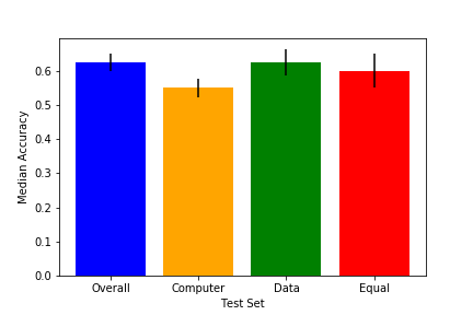
We consider the first two conditions to be the ‘Data’ group, the third to be the ‘Equal’ group, and the next two to be the ‘Computer Advice’ group. Although the trend is not statistically significant (at $p=0.05$), likely due to the small number of subjects per type per round, we find it interesting that the performance improved on average over training rounds for all three types, of which the equal-consideration type performed best. For the data-inclined users, whose performance improved to surpass that of the no-advice condition in as early as round two, this implies at least one of the following: users misreport their decision method; users believe they are not influenced by the advice but are in fact influenced; or, as the algorithmic evidence becomes apparently better, only the population of users who are comparatively skilled at using the data continue to do so.

C.2.4 Diversity in avatar representation.

Figure 10 presents examples of visualized avatars. Avatars correspond to examples having either low or high human-predicted probability (averaged across users) (top figure), and either low or high machine-predicted probability (lower figure). For visualization purposes, avatars are aligned according to a uni-dimensional PCA projection of the inputs, so that their spatial positioning captures the variance in the data. As can be seen, avatars are different for each predictive category (positive or negative; human or machine), but also vary considerably within each predictive category, with variance eminent across multiple facial dimensions.

We believe the additional dimensionality of the avatar representation relative to a numerical or binary prediction of default is useful for two reasons. Most importantly, high dimensionality allows users to retain an ability to reason about their decisions. In particular, avatars are useful because people likely have shared, mental reference points for faces. Moreover, users with a more sophisticated mental reference space may be able to teach the advising system over time to match specific reasoning patterns to specific characteristics. Additionally, when the advising system does not have a strong conviction about a prediction, presenting neutral advice should encourage the user to revisit the data, whereas percentages above or below the base rate of default (or 50%) may suffer from the anchoring effect.

C.2.5 Further Details on Information Learned by $z$.

Using cross-validated ridge regression to predict individual $x$ variables from individual $z$ variables results in the coefficients of determination $R^{2}$ (to 2 significant figures) shown in Table 2.

Using cross-validated ridge regression to predict individual $x$ variables from all $z$ variables (both standardized to mean 0, std 1) results in the variable coefficients (to 2 significant figures) shown in Table 3.

See mom_fig10_1page.pdf

C.3 Incorporating Side Information

C.3.1 Data Generation.

A directed graph showing the variable correlations is shown in Figure 11. The data in the side-information experiment is generated as follows: A latent variable $l_{0}\sim\mathcal{N}(.3,.1)$ introduces a low correlation between $x_{i}$ and $x_{r}$ by setting a common mean for their Bernoulli probabilities $l_{1},l_{2}$:

• $l_{1},l_{2}\sim\textrm{Unif}(\textrm{max}(l_{0}-.3,0),\textrm{min}(l_{0}+.3,1))$

• $x_{i}\sim\textrm{Bernoulli}(1-l_{1})$

• $x_{r}\sim\textrm{Bernoulli}(1-l_{2})$

An additional latent variable $l_{3}$ provides a similar correlation between $x_{c}$ and $x_{d}$, which also correlate, respectively, with $x_{i}$ and $x_{r}$:

• $l_{3}\sim\textrm{Unif}(.5,.7)$

• $x_{c}\sim\textrm{Bernoulli}(l_{3}+x_{i})$

• $x_{d}\sim\textrm{Bernoulli}(l_{3}+x_{r})$

Side information $s$ is highly correlated with $x_{r}$ and $x_{i}$ but noisy: $s$ is drawn from a normal distribution centered at $x_{r}+x_{i}$ before rounding to an integer value between 0 and 3.

• $s_{cont}\sim\mathcal{N}(x_{r}+x_{i},.5)$

• $s=\textrm{max}(0,\textrm{min}(3,\textrm{round}(s_{cont})))$

The integer outcome variable $y$ is the sum of $x_{c}$, $x_{d}$, and $s$. The binary outcome variable $y_{bin}$ is thresholded at $y>3$.

$y=x_{c}+x_{d}+s$; $;\ y_{bin}=\mathds{1}{\{{y>3}\}}$

Table 2: Coefficients of Determination $R^{2}$, predicting each $x$ variable from each final $z$ variable.

	rate	term	dt	rec	inc	emp [b]
happiness	0.00	-0.15	-0.14	0.00	-0.01	0.00 [t]
sadness	-0.01	-0.06	-0.10	0.00	-0.04	-0.07
trustworthiness	0.57	0.17	0.01	0.00	-0.01	-0.01
dominance	0.00	-0.01	0.03	-0.01	0.01	-0.01
hue	0.48	0.29	-0.02	0.00	-0.04	-0.02
eye gaze	0.42	0.46	-0.04	-0.40	-0.04	-0.17
age	0.23	0.22	-0.12	-0.21	0.17	0.04
anger	-0.01	-0.02	-0.05	-0.02	-0.01	0.00
fear	0.04	0.00	-0.03	0.00	-0.01	-0.01
surprise	-0.18	0.04	-0.01	-0.02	0.00	-0.04

Table 3: Coefficients of Ridge Regression, predicting each $x$ variable from all final $z$ variables.

	rate	term	dt	rec	inc	emp [b]
happiness	-0.07	-0.29	-0.10	-0.06	0.21	-0.07 [t]
sadness	0.16	0.07	0.07	-0.01	0.13	0.07
trustworthiness	-0.62	-0.28	-0.05	-0.23	0.31	0.16
dominance	0.05	0.16	0.12	-0.13	-0.02	0.04
hue	0.27	0.20	0.19	0.03	0.01	-0.08
eye gaze	0.13	0.28	-0.10	0.13	-0.29	-0.04
age	-0.09	0.14	0.12	-0.09	0.67	0.40
anger	0.00	0.00	0.00	0.00	0.00	0.00
fear	0.19	0.12	0.08	-0.07	0.04	0.00
surprise	0.07	0.12	0.03	-0.07	-0.06	0.13

Figure 11: Relationship of variable correlations in the side information experiment

C.3.2 Learning Architecture.

The network ${\phi}$ contains a single linear layer with no bias which takes a constant (1) as an input and outputs a number $z_{i}$ for each data dimension $i$.

The network ${\hat{h}}$ takes as input $(x,w,y)$. It contains one linear layer with no bias which takes as input $[x,y]$ and outputs a single number $\hat{s}$. The second linear layer (with bias) takes as input $w$ and outputs the sigmoid activation of a single number, $switch$, representing the propensity to incorporate $s$ at $w$. It then outputs $w^{\intercal}x+switch\cdot\hat{s}$.

C.3.3 Baselines.

• Machine Only: The best possible linear model (with bias) trained to predict $y$ from $x_{1}\ldots x_{4}$.

• $h($Machine): The human model $h$ applied to the best possible linear model (with bias) trained to predict $y$ from $x_{1}\ldots x_{4}$.

  $$h(\text{Machine})=\beta_{0}+h(x,\beta_{1},\dots,\beta_{4},s)$$

  where $\beta$ are the coefficients selected by the machine-only regression.

C.3.4 Human Models

• Always: The human always fully incorporates the side information,

  $$h(x,w,s)=w^{\intercal}x+s$$

• Never: The human never incorporates the side information,

  $$h(x,w,s)=w^{\intercal}x$$

• Or: The human becomes less likely to incorporate side information as weight is put on $x_{i},x_{r}$,

  $$h(x,w,s)=w^{\intercal}x+\sigma(1/\textrm{max}(\textrm{max}(x_{i},x_{r}),.0001)-2).\cdot s$$

  Note that max(.0001) is required to prevent numerical overflow, and -2 recenters the sigmoid to allow for values $<.5$.

• Coarse: The human incorporates $s$ as in Or, but uses a coarse, noisy version of $s$, $s^{\prime}=2\cdot\mathds{1}{\{{s\geq 2}\}}$

  $$h(x,w,s)=w^{\intercal}x+\sigma(1/\textrm{max}(\textrm{max}(x_{i},x_{r}),.0001)-2).\cdot s^{\prime}$$

Appendix D Select Turker quotes

• “I wasn’t always looking at just happiness or sadness. Sometimes the expressions seemed disingenuously happy, and that also threw me off. I don’t know if that was intentional but it definitely effected my gut feeling and how I chose.”

• “In my opinion, the level of happiness or sadness, the degree of a smile or a frown, was used to represent applications who were likely to be payed back. The more happy one looks, the better the chances of the client paying the loan off (or at least what the survey information lead me to believe).”

• “I was more comfortable with facial expressions than numbers. I felt like a computer and I didn’t feel human anymore. Didn’t like it at all.”

References

- Amershi et al. (2014) Amershi, S., Cakmak, M., Knox, W. B., and Kulesza, T. Power to the people: The role of humans in interactive machine learning. Ai Magazine, 35(4):105–120, 2014.
- Arjovsky et al. (2017) Arjovsky, M., Chintala, S., and Bottou, L. Wasserstein gan. arXiv preprint arXiv:1701.07875, 2017.
- Bandura (1989) Bandura, A. Human agency in social cognitive theory. American psychologist, 44(9):1175, 1989.
- Bandura (2010) Bandura, A. Self-efficacy. The Corsini encyclopedia of psychology, pp. 1–3, 2010.
- Bansal et al. (2019) Bansal, G., Nushi, B., Kamar, E., Lasecki, W. S., Weld, D. S., and Horvitz, E. Beyond accuracy: The role of mental models in human-ai team performance. In Proc. AAAI Conf. on Human Comput. and Crowdsourcing, 2019.
- Bansal et al. (2020) Bansal, G., Wu, T., Zhu, J., Fok, R., Nushi, B., Kamar, E., Ribeiro, M. T., and Weld, D. S. Does the whole exceed its parts? the effect of ai explanations on complementary team performance. arXiv preprint arXiv:2006.14779, 2020.
- Barabas et al. (2017) Barabas, C., Dinakar, K., Ito, J., Virza, M., and Zittrain, J. Interventions over predictions: Reframing the ethical debate for actuarial risk assessment. arXiv preprint arXiv:1712.08238, 2017.
- Bengio et al. (2013) Bengio, Y., Courville, A., and Vincent, P. Representation learning: A review and new perspectives. IEEE transactions on pattern analysis and machine intelligence, 35(8):1798–1828, 2013.
- Berdichevsky & Neuenschwander (1999) Berdichevsky, D. and Neuenschwander, E. Toward an ethics of persuasive technology. Comm. ACM, 42(5):51–58, 1999.
- Bourgin et al. (2019) Bourgin, D. D., Peterson, J. C., Reichman, D., Griffiths, T., and Russell, S. J. Cognitive model priors for predicting human decisions. arXiv preprint arXiv:1905.09397, 2019.
- Brown et al. (2013) Brown, J. R., Kling, J. R., Mullainathan, S., and Wrobel, M. V. Framing lifetime income. Technical report, National Bureau of Economic Research, 2013.
- Chernoff (1973) Chernoff, H. The use of faces to represent points in k-dimensional space graphically. JASA, 68(342):361–368, 1973.
- Cosmides & Tooby (1992) Cosmides, L. and Tooby, J. Cognitive adaptations for social exchange. The adapted mind: Evolutionary psychology and the generation of culture, 163:163–228, 1992.
- Cramer et al. (2008) Cramer, H., Evers, V., Ramlal, S., Van Someren, M., Rutledge, L., Stash, N., Aroyo, L., and Wielinga, B. The effects of transparency on trust in and acceptance of a content-based art recommender. User Modeling and User-adapted interaction, 18(5):455, 2008.
- De-Arteaga et al. (2020) De-Arteaga, M., Fogliato, R., and Chouldechova, A. A case for humans-in-the-loop: Decisions in the presence of erroneous algorithmic scores. In Proc. 2020 CHI Conf. on Human Factors in Computing Systems, pp. 1–12, 2020.
- DeBruine & Tiddeman (2016) DeBruine, L. and Tiddeman, B. Webmorph, 2016.
- Dietvorst et al. (2015) Dietvorst, B. J., Simmons, J. P., and Massey, C. Algorithm aversion: People erroneously avoid algorithms after seeing them err. Journal of Experimental Psychology: General, 144(1):114, 2015.
- Dietvorst et al. (2016) Dietvorst, B. J., Simmons, J. P., and Massey, C. Overcoming algorithm aversion: People will use imperfect algorithms if they can (even slightly) modify them. Management Science, 64(3):1155–1170, 2016.
- Du et al. (2014) Du, S., Tao, Y., and Martinez, A. M. Compound facial expressions of emotion. Proceedings of the National Academy of Sciences, 111(15):E1454–E1462, 2014.
- Elmalech et al. (2015) Elmalech, A., Sarne, D., Rosenfeld, A., and Erez, E. S. When suboptimal rules. In Twenty-Ninth AAAI Conference on Artificial Intelligence, 2015.
- Engelbart (1962) Engelbart, D. C. Augmenting human intellect: A conceptual framework. Menlo Park, CA, 1962.
- Esteva et al. (2017) Esteva, A., Kuprel, B., Novoa, R. A., Ko, J., Swetter, S. M., Blau, H. M., and Thrun, S. Dermatologist-level classification of skin cancer with deep neural networks. Nature, 542(7639):115, 2017.
- Fogg (1998) Fogg, B. J. Persuasive computers: perspectives and research directions. In Proceedings of the SIGCHI conference on Human factors in computing systems, pp. 225–232, 1998.
- Freeman & Johnson (2016) Freeman, J. B. and Johnson, K. L. More than meets the eye: Split-second social perception. Trends in cognitive sciences, 20(5):362–374, 2016.
- Gigerenzer & Hoffrage (1995) Gigerenzer, G. and Hoffrage, U. How to improve bayesian reasoning without instruction: frequency formats. Psychological review, 102(4):684, 1995.
- Green & Chen (2019a) Green, B. and Chen, Y. Disparate interactions: An algorithm-in-the-loop analysis of fairness in risk assessments. In Proc. ACMFAT Conf. ACM, 2019a.
- Green & Chen (2019b) Green, B. and Chen, Y. The principles and limits of algorithm-in-the-loop decision making. Proceedings of the ACM on Human-Computer Interaction, 3(CSCW):1–24, 2019b.
- Izard (1994) Izard, C. E. Innate and universal facial expressions: Evidence from developmental and cross-cultural research. Psychological Bulletin, 115(2):288–299, 1994.
- Kahneman (2011) Kahneman, D. Thinking, fast and slow. Macmillan, 2011.
- Kahneman & Tversky (2013) Kahneman, D. and Tversky, A. Prospect theory: An analysis of decision under risk. In Handbook of the fundamentals of financial decision making: Part I, pp. 99–127. World Scientific, 2013.
- Kiselev et al. (2019) Kiselev, V. Y., Andrews, T. S., and Hemberg, M. Challenges in unsupervised clustering of single-cell rna-seq data. Nature Reviews Genetics, 20(5):273–282, 2019.
- Kleinberg et al. (2015) Kleinberg, J., Ludwig, J., Mullainathan, S., and Obermeyer, Z. Prediction policy problems. American Economic Review, 105(5):491–95, 2015.
- Lage et al. (2018) Lage, I., Ross, A., Gershman, S. J., Kim, B., and Doshi-Velez, F. Human-in-the-loop interpretability prior. In Adv. in Neural Info. Proc. Sys., pp. 10159–10168, 2018.
- Lage et al. (2019) Lage, I., Chen, E., He, J., Narayanan, M., Kim, B., Gershman, S. J., and Doshi-Velez, F. Human evaluation of models built for interpretability. In Proceedings of the AAAI Conference on Human Computation and Crowdsourcing, volume 7, pp. 59–67, 2019.
- Lai & Tan (2018) Lai, V. and Tan, C. On human predictions with explanations and predictions of machine learning models: A case study on deception detection. arXiv preprint arXiv:1811.07901, 2018.
- Lai & Tan (2019) Lai, V. and Tan, C. On human predictions with explanations and predictions of machine learning models: A case study on deception detection. In Proceedings of the Conference on Fairness, Accountability, and Transparency, pp. 29–38, 2019.
- Lai et al. (2020) Lai, V., Carton, S., and Tan, C. Harnessing explanations to bridge ai and humans. arXiv preprint arXiv:2003.07370, 2020.
- Lakkaraju et al. (2016) Lakkaraju, H., Bach, S. H., and Leskovec, J. Interpretable decision sets: A joint framework for description and prediction. In Proc. 22nd ACM SIGKDD Int. Conf. on Know. Disc. and Data Mining, pp. 1675–1684. ACM, 2016.
- Licklider (1960) Licklider, J. C. R. Man-computer symbiosis. IRE transactions on human factors in electronics, pp. 4–11, 1960.
- Liu et al. (2019) Liu, X., Faes, L., Kale, A. U., Wagner, S. K., Fu, D. J., Bruynseels, A., Mahendiran, T., Moraes, G., Shamdas, M., Kern, C., et al. A comparison of deep learning performance against health-care professionals in detecting diseases from medical imaging: a systematic review and meta-analysis. The Lancet Digital Health, 1(6):e271–e297, 2019.
- Logg (2017) Logg, J. M. Theory of machine: When do people rely on algorithms?, 2017.
- Lott & Durbridge (1990) Lott, J. A. and Durbridge, T. C. Use of chernoff faces to follow trends in laboratory data. Journal of clinical laboratory analysis, 4(1):59–63, 1990.
- Lundberg & Lee (2017) Lundberg, S. M. and Lee, S.-I. A unified approach to interpreting model predictions. In Advances in Neural Information Processing Systems, 2017.
- Lurie & Mason (2007) Lurie, N. H. and Mason, C. H. Visual representation: Implications for decision making. Journal of marketing, 71(1):160–177, 2007.
- Madras et al. (2018) Madras, D., Pitassi, T., and Zemel, R. Predict responsibly: Improving fairness and accuracy by learning to defer. In Adv. in Neural Info. Proc. Sys. 31, pp. 6147–6157. 2018.
- Miller (1956) Miller, G. A. The magical number seven, plus or minus two: Some limits on our capacity for processing information. Psychological review, 63(2):81, 1956.
- Mozannar & Sontag (2020) Mozannar, H. and Sontag, D. Consistent estimators for learning to defer to an expert. In International Conference on Machine Learning, pp. 7076–7087. PMLR, 2020.
- Nickerson & Rogers (2014) Nickerson, D. W. and Rogers, T. Political campaigns and big data. J. Econ. Persp., 28(2):51–74, 2014.
- Parikh et al. (2019) Parikh, R. B., Obermeyer, Z., and Navathe, A. S. Regulation of predictive analytics in medicine. Science, 363(6429):810–812, 2019.
- Poursabzi-Sangdeh et al. (2018) Poursabzi-Sangdeh, F., Goldstein, D. G., Hofman, J. M., Vaughan, J. W., and Wallach, H. Manipulating and measuring model interpretability. arXiv preprint arXiv:1802.07810, 2018.
- Ribeiro et al. (2016) Ribeiro, M. T., Singh, S., and Guestrin, C. Why should i trust you?: Explaining the predictions of any classifier. In Proc. 22nd ACM SIGKDD Int. Conf. on Know. Disc. and Data Mining, pp. 1135–1144. ACM, 2016.
- Richler et al. (2009) Richler, J. J., Mack, M. L., Gauthier, I., and Palmeri, T. J. Holistic processing of faces happens at a glance. Vision research, 49(23):2856–2861, 2009.
- Ross et al. (2017) Ross, A. S., Hughes, M. C., and Doshi-Velez, F. Right for the right reasons: Training differentiable models by constraining their explanations. arXiv preprint arXiv:1703.03717, 2017.
- Stevenson & Doleac (2018) Stevenson, M. and Doleac, J. Algorithmic risk assessment tools in the hands of humans, 2018.
- Stevenson & Doleac (2019) Stevenson, M. T. and Doleac, J. L. Algorithmic risk assessment in the hands of humans. SSRN, 2019.
- Sutton et al. (2020) Sutton, R. T., Pincock, D., Baumgart, D. C., Sadowski, D. C., Fedorak, R. N., and Kroeker, K. I. An overview of clinical decision support systems: benefits, risks, and strategies for success. NPJ Digital Medicine, 3(1):1–10, 2020.
- Tabibian et al. (2019) Tabibian, B., Upadhyay, U., De, A., Zarezade, A., Schölkopf, B., and Gomez-Rodriguez, M. Enhancing human learning via spaced repetition optimization. Proc. Nat. Acad. of Sci., 116(10):3988–3993, 2019.
- Thompson (1980) Thompson, P. Margaret thatcher: A new illusion. Perception, 1980.
- Todorov et al. (2008) Todorov, A., Said, C. P., Engell, A. D., and Oosterhof, N. N. Understanding evaluation of faces on social dimensions. Trends in cognitive sciences, 12(12):455–460, 2008.
- Venkatesh et al. (2003) Venkatesh, V., Morris, M. G., Davis, G. B., and Davis, F. D. User acceptance of information technology: Toward a unified view. MIS quarterly, pp. 425–478, 2003.
- West & Crawford (2019) West, S.M. Whittaker, M. and Crawford, K. Discriminating systems: Gender, race and power in ai., 2019. URL https://ainowinstitute.org/discriminatingsystems.html.
- Wilder et al. (2020) Wilder, B., Horvitz, E., and Kamar, E. Learning to complement humans. arXiv preprint arXiv:2005.00582, 2020.
- Yeomans et al. (2017) Yeomans, M., Shah, A., Mullainathan, S., and Kleinberg, J. Making sense of recommendations. Journal of Behavioral Decision Making, 2017.
- Yin et al. (2019) Yin, M., Vaughan, J. W., and Wallach, H. M. Understanding the effect of accuracy on trust in machine learning models. In Proceedings of the 2019 Conference on Human Factors in Computing Systems, 2019.