Waveguide Modes in Weyl Semimetals with Tilted Dirac Cones

Abstract

We theoretically study unattenuated electromagnetic guided wave modes in centrosymmetric Weyl semimetal layered systems. By solving Maxwell’s equations for the electromagnetic fields and using the appropriate boundary conditions, we derive dispersion relations for propagating modes in a finite-sized Weyl semimetal. Our findings reveal that for ultrathin structures, and proper Weyl cones tilts, extremely localized guided waves can propagate along the semimetal interface over a certain range of frequencies. This follows from the anisotropic nature of the semimetal where the diagonal components of the permittivity can exhibit a tunable epsilon-near-zero response. From the dispersion diagrams, we determine experimentally accessible regimes that lead to high energy-density confinement in the Weyl semimetal layer. Furthermore, we show that the net system power can vanish all together, depending on the Weyl cone tilt and frequency of the electromagnetic wave. These effects are seen in the energy transport velocity, which demonstrates a substantial slowdown in the propagation of electromagnetic energy near critical points of the dispersion diagrams. Our results can provide guidelines in designing Weyl semimetal waveguides that can offer efficient control in the velocity and direction of energy flow.

1 Introduction

With the recent discoveries of a number of Weyl[1] semimetal (WS) compounds[14, 5, 7, 8, 9, 18, 16, 10, 15, 6, 17, 4, 11, 13, 12, 2, 3] and their intriguing optical properties [36, 35, 34, 19, 27, 23, 32, 29, 33, 24, 20, 31, 28, 4, 30, 22, 21, 26, 25], there has been a surge in research that investigates their potential roles in future optical systems. When studying the electromagnetic (EM) properties of WS systems, it is important to take into consideration their inherent anisotropic nature. Depending on the polarization of the EM wave relative to the crystalline axes, a WS can be tuned to exhibit a metallic or insulating type of EM response, as described by its permittivity tensor $\overline{\overline{\epsilon}}$. This is reflected in the real parts of the appropriate components of $\overline{\overline{\epsilon}}$ changing sign, or vanishing altogether, as occurs in epsilon-near-zero (ENZ) materials [49, 41, 37, 38, 39, 40, 42, 43, 44, 45, 46, 47, 48]. Various peculiar effects can arise in materials exhibiting an ENZ response [46], including light tunneling, vanishing group velocity, and perfect absorption [43]. By exploiting the anisotropic tunable EM response of Weyl semimetals, new classes of optical devices, such as waveguides, can be designed that afford dissipationless, highly localized energy transport with minimal attenuation and signal distortion.

For anisotropic waveguides, the relative signs of the components of $\overline{\overline{\epsilon}}$ can also be crucial for the optimization of energy transport. For example, a uniaxial anisotropic system that has permittivities of opposite sign can have an isofrequency surface in the form of an open hyperboloid. Such hyperbolic metamaterials have been discussed in the context of waveguides[50] to generate forward and backward surface modes [51], and to enhance EM fields [52]. Thus, the anisotropic EM response of a WS must be accounted for when discussing its role as a waveguide in the ENZ regime. Indeed, the sign differences that can arise between the diagonal permittivity components, can afford greater control and increased subwavelength EM field confinement.

In addition to the dielectric response of Weyl semimetals, the tilting of the Weyl cones can induce observable effects in the conductivity and polarization [32]. By reversing the conical tilt direction, the right-hand and left-hand responses of the Weyl semimetal become reversed, which can affect the absorption of circularly polarized light [29]. It was found that the chirality or sign of the tilt parameter in the absence of time-reversal and inversion symmetries can change the sign of the Weyl contributions to the absorptive Hall conductivity [33]. For Weyl semimetal structures much thinner than the incident wavelength, EM radiation can be perfectly absorbed for nearly any incident angle, depending on the tilt of the Weyl cones and chemical potential [48]. Moreover, the broad tunability of the chemical potential in a WS makes it a promising material for photonics and plasmonics applications[54, 55, 56, 57, 24, 26, 53, 25, 18, 20]. The chiral anomaly in a WS can alter surface plasmons and the EM response [54, 55, 56, 57, 24, 25, 26]. Other interesting optical effects can also arise in Weyl semimetals, including the Imbert-Fedorov effect, which can result in detectable valley-dependent variations in the velocites of Weyl fermions [58]. It has been shown theoretically [26] that measurements of the optical conductivity and the temperature dependence of the free carrier response in pyrochlore Eu₂Ir₂O₇ is consistent with the WS phase, and that the interband optical conductivity reduces to zero in a continuous fashion at low frequencies as predicted for a WS. The surface magnetoplasmons of a Weyl semimetal can turn to low-loss localized guided modes when two crystals of the WSs with different magnetization orientations are connected [24].

In this paper, we investigate guided wave modes that can arise in an anisotropic Weyl semimetal waveguide structure. We consider a finite-sized Weyl semimetal layer on top of a perfectly conducting substrate. Our study includes both analytic and numerical results that determine the EM fields and characteristics of the energy flow in WS waveguide systems. We consider broad ranges of conical tilting, and EM wave frequencies. We show that by appropriately tuning the frequency and conical tilt, both of the diagonal components of $\overline{\overline{\epsilon}}$ can achieve a lossless ENZ response. From the obtained dispersion relations, which reveal the permitted EM solutions, we construct the EM fields and identify regions of high energy density confinement in the WS layer. We demonstrate controllable net system power that can be made to vanish at critical points of the dispersion curves, where the propagation of electromagnetic energy comes to a standstill. Our findings offer systematic ways to design waveguide structures that can continuously reduce the energy velocity from a fraction of the speed of light to effectively zero.

The paper is organized as follows: In Sec. 2.1, we summarize the dielectric response of the WS by presenting each component of the permittivity tensor, and give details of the approximations made. Next, in Sec. 2.2, we solve Maxwell’s equations and obtain the dispersion relations for the corresponding guided EM wave modes. We also define the averaged energy density, Poynting vector, and velocity of energy flow. In Sec. 2.3, we examine the obtained analytical expressions numerically and discuss our main results. Finally in Sec. 3, we give concluding remarks.

2 Model and results

In this section, we outline the salient features of the EM response of a WS by providing analytical expressions for the components of the permittivity tensor, as well as the numerical approach used. For clarity, we have considered the zero temperature case, and neglect the influence of impurities and disorder. At finite temperatures, or the presence of impurities and disorder, the mode dispersion diagram would acquire additional radiative mode characteristics. For high enough temperatures, optical absorption and propagating modes would be dominated less by coherent interference effects and more by dissipative ones, adversely impacting the findings presented here. The Weyl semimetal is modeled as a system with broken time-reversal symmetry and two Weyl nodes. This model can be achieved through the stacking of multiple thin films involving a topological insulator and ferromagnet blocks [4]. The Hamiltonian describing the low energy physics around the two Weyl nodes, defined by “$s=\pm$”, is given by:

$$H_{s}(\mathbf{p})=v_{F}[\beta_{s}(p_{z}-sQ)+s{\bm{\sigma}}(\textbf{p}-sQ\textbf{e}_{z})].$$ (1)

Here $\textbf{e}_{z}$ is the unit vector along the $z$ direction, and we take the Fermi velocity $v_{F}$ to be positive. The separation between two Weyl points in the $z$ direction in momentum space is defined by $2|Q|$, where the sign of $Q$ depends on the sign of the magnetization. The tilt of the Weyl cones are described by the parameters $\beta_{\pm}$, and for centrosymmetric materials with broken time reversal symmetry, we apply the condition $\beta=\beta_{+}=-\beta_{-}$.

2.1 Permittivity tensor

The permittivity tensor $\overline{\overline{\epsilon}}$ for the WS takes the following gyrotropic form:[48]

$$\overline{\overline{\epsilon}}(\omega)=\left(\begin{array}[]{ccc}\epsilon_{\parallel}(\omega)&i\gamma(\omega)&0\\ -i\gamma(\omega)&\epsilon_{\parallel}(\omega)&0\\ 0&0&\epsilon_{zz}(\omega)\end{array}\right),$$ (5)

where $\epsilon_{\parallel}(\omega)$ represents the equal components of ${\overline{\overline{\epsilon}}}(\omega)$ parallel to the interfaces, i.e., $\epsilon_{xx}(\omega)=\epsilon_{yy}(\omega)=\epsilon_{\parallel}(\omega)$. Here the components are normalized by $\epsilon_{0}$, the permittivity of free space. The $\epsilon_{\parallel}(\omega)$ components can be written analytically as [48],

$$\epsilon_{\parallel}(\omega)=1+\frac{\alpha}{3\pi}\left[\text{ln}\left|\dfrac{4\Gamma^{2}}{4\mu^{2}-\omega^{2}}\right|-\dfrac{4\mu^{2}}{\omega^{2}}+i\pi\Theta(\omega-2\mu)\right],$$ (6)

where $\mu$ is the chemical potential, with $\mu\geq 0$, $\alpha=e^{2}/(4\pi\epsilon_{0}\hbar v_{F})$, and $\Theta(X)$ represents the usual step function. Generally, the energy cut-off $\Gamma$ is a function of the tilt parameter. Nevertheless, in our calculations, we choose a large enough cut-off and neglect the contribution of $\beta_{\pm}$ to $\Gamma$.

It is evident that $\epsilon_{\parallel}(\omega)$ is independent of the tilting parameters $\beta_{\pm}$. For the situation when the Weyl cones are not tilted ($\beta_{\pm}=0$), we have $\epsilon_{zz}(\omega)=\epsilon_{\parallel}(\omega)$, and the off-diagonal frequency dependent component $\gamma(\omega)$ reduces to, $\gamma(\omega)=2v_{F}\alpha Q(\pi\omega)^{-1}$. The imaginary term in Eq. (6) describes the interband contribution to the optical conductivity, which exists only when the frequency $\omega$ of the EM wave satisfies $\omega>2\mu$. For the guided waves of interest, we are interested in the situation where there is no dissipation in the medium. As Eq. (6) shows, the range of frequencies in which $\epsilon_{\parallel}$ is real and positive corresponds to

$$2\mu\sqrt{\frac{\alpha}{3\pi+{2\alpha}\ln{\big{|}{\Gamma}/{\mu}\big{|}}}}<\omega<2\mu.$$ (7)

Similarly, the permittivity component $\epsilon_{zz}$ depends on frequency and chemical potential, however it also depends on the tilt $\beta_{\pm}$. The $\epsilon_{zz}$ component involves a complicated integral, and its derivation is presented elsewhere [48]. For frequencies satisfying

$$\omega<\frac{2\mu}{(1+|\beta|)},$$ (8)

there is no dissipation (for all diagonal components), and $\epsilon_{zz}$ can be written analytically as [48],

$$\epsilon_{zz}=1+\frac{\alpha\mu^{2}}{\pi\omega^{2}} \sum\limits_{s=\pm}\frac{1}{\beta_{s}^{3}}\Bigg{\{}\frac{8}{3}\beta_{s}-4\operatorname{arctanh}\beta_{s}+\ln\bigg{|}\frac{4\mu^{2}-\omega^{2}(1+\beta_{s})^{2}}{4\mu^{2}-\omega^{2}(1-\beta_{s})^{2}}\bigg{|}$$

$$+\frac{\omega^{2}}{12\mu^{2}} \sum\limits_{t=\pm 1}\Bigg{[}t\Big{(}1+2t\beta_{s}\Big{)}\Big{(}1-t\beta_{s}\Big{)}^{2}\ln\bigg{|}\frac{4\Gamma^{2}(1-t\beta_{s})^{2}}{4\mu^{2}-\omega^{2}(1-t\beta_{s})^{2}}\bigg{|}$$

$$-\frac{2\mu}{\omega}\Big{(}\frac{4\mu^{2}}{\omega^{2}}+3-3\beta_{s}^{2})\ln\bigg{|}\frac{2\mu-t\omega(1+t\beta_{s})}{2\mu+t\omega(1+t\beta_{s})}\bigg{|}\Bigg{]}\Bigg{\}},$$ (9)

which is valid for $|\beta_{\pm}|<1$. Below, we show that over a range of frequencies, $\epsilon_{zz}$ and $\epsilon_{\parallel}$ can be tuned to achieve an ENZ response at different $\omega$. We also show that there are a range of frequencies where $\epsilon_{\parallel}$ and $\epsilon_{zz}$ can have opposite signs, which strongly affects the types of modes that will propagate along the waveguide interface. Here we have neglected the effects of electron scattering on the absorption. Increasing the dissipation in the diagonal components of the permittivity tensor can result in the generation of other types of waveguide modes, including leaky waves [41], which fall outside the scope of this paper.

The remaining off-diagonal term $\gamma$ can play an important role in changing the polarization state of EM waves interacting with the WS via Faraday and Kerr rotations [23, 27]. Variations in the gyrotropic term can also cause shifts in the surface plasmon frequency [59]. The gyrotropic term can be written analytically in the limit $\omega\rightarrow 0$:

$$\gamma=\frac{\alpha}{\pi\omega}\bigg{[}2v_{F}Q-\sum_{s=\pm}\frac{s\mu}{2\beta_{s}}\bigg{(}\frac{1}{\beta_{s}}\ln\bigg{|}\frac{1+\beta_{s}}{1-\beta_{s}}\bigg{|}-2\bigg{)}\bigg{]},|\beta_{s}|\ll 1.$$ (10a)

Thus, for fixed $\beta$, and small tilting, $\gamma$ is a linear function of $\mu$, declining as the chemical potential increases. For arbitrary $\beta$ and $\omega$, it is necessary to resort to numerics to determine $\gamma$ (see Appendix).

We now make use of the expressions above governing the relevant components of ${\overline{\overline{\epsilon}}}$ to demonstrate that by properly tailoring the EM response, the waveguide structure can effectively transport localized EM energy over a broad range of frequencies and tilting of the Weyl cones ( $0<\beta<1$), where we recall $\beta_{+}=-\beta_{-}=\beta$. When characterizing the nontrivial behavior of $\overline{\overline{\epsilon}}$ in the WS, there are several relevant parameters to consider, including the chemical potential, frequency of the EM wave, tilt of the Weyl cones, and the node separation parameter $Q$ (which is taken to be positive).

2.2 Guided wave modes and energy confinement

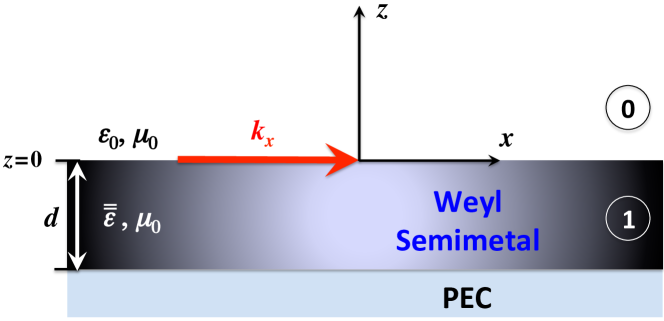
Figure 1: Schematic of the waveguide configuration involving a Weyl semimetal (in region $1$) with width $d$ on top of a perfectly conducting substrate. In this configuration, the wavevector ${\bm{k}}$ resides in the plane of the WS (along $x$), while the separation of Weyl nodes is perpendicular to the layers (along $z$). The surrounding medium (region $0$) is taken to be vacuum.

We now investigate the EM modes for the configuration shown in Fig. 1, which consists of a planar Weyl semimetal (region $1$) adjacent to a metallic substrate with perfect conductivity (PEC). The propagation constant $k_{x}$ is invariant across each layer. For both regions $0$ and $1$, we implement Maxwell’s equations for time harmonic fields,

$${\bm{\nabla}}\times{\bm{E}}_{i} =i\omega\mu_{0}{\bm{H}}_{i},$$ (11a)

$${\bm{\nabla}}\times{\bm{H}}_{i} =-i\omega{\bm{D}}_{i},$$ (11b)

where $i=0$ or $1$. Within the WS, the propagation vector ${\bm{k}}_{1}$ replaces the spatial derivatives, transforming Maxwell’s equations into the forms, ${\bm{k}}_{1}\times{\bm{E}}_{1}=\omega\mu_{0}{\bm{H}}_{1}$ and ${\bm{k}}_{1}\times{\bm{H}}_{1}=-\omega{\overline{\overline{\epsilon}}}\epsilon_{0}{\bm{E}}_{1}$. These two equations together result in the following expression for the ${\bm{E}}_{1}$ field in $\bm{k}$-space:

$${\bm{k}}_{1}\times({\bm{k}}_{1}\times{\bm{E}}_{1})=-k_{0}^{2}{\overline{\overline{\epsilon}}}{\bm{E}}_{1}.$$ (12)

Using ${\bm{k}}_{1}=k_{x}\hat{\bm{x}}+k_{1z}\hat{\bm{z}}$, and the identity ${\bm{k}}_{1}\times({\bm{k}}_{1}\times{\bm{E}}_{1})={\bm{k}}_{1}({\bm{k}}_{1}{\bm{E}}_{1})-k_{1}^{2}{\bm{E}}_{1}$, permits expansion of Eq. (12),

$$\begin{pmatrix}k_{0}^{2}\epsilon_{xx}-k_{1z}^{2}&ik_{0}^{2}\gamma&k_{1z}k_{x}\\ ik_{0}^{2}\gamma&k_{\perp}^{2}-k^{2}_{0}\epsilon_{yy}&0\\ k_{x}k_{1z}&0&k_{0}^{2}\epsilon_{zz}-k_{x}^{2}\end{pmatrix}\begin{pmatrix}E_{x1}\\ E_{y1}\\ E_{z1}\end{pmatrix}=0,$$ (13)

where $k_{0}=\omega/c$, and $k_{\perp}=\sqrt{k_{1z}^{2}+k_{x}^{2}}$. Due to translational invariance, we also have $k_{1x}=k_{x}$. The presence of all three $\bm{E}$ field components in Eq. (13) is a consequence of the centrosymmetrc nature of the WS that can couple different polarization states, depending on the WS material parameters and layer width.

Taking the determinant of the matrix in Eq. (13) and setting it equal to zero, gives the dispersion equation for the wavevector $k_{1z}$ in the semimetal:

$$(\epsilon_{xx}k_{0}^{2}-k_{\perp}^{2})(\epsilon_{xx}\epsilon_{zz}k_{0}^{2}-\epsilon_{xx}k_{x}^{2}-\epsilon_{zz}k_{1z}^{2})+k_{0}^{2}(k_{x}^{2}-\epsilon_{zz}k_{0}^{2})\gamma^{2}=0.$$ (14)

Solving Eq. (14) for $k_{1z}$ results in two types of solutions denoted by $k_{+}$ and $k_{-}$:

$$k_{\pm}=\pm\sqrt{\frac{k_{0}^{2}}{2\epsilon_{zz}}\Biggl{(}2\epsilon_{zz}\epsilon_{\parallel}-(\epsilon_{\parallel}+\epsilon_{zz})\kappa_{x}^{2}\pm\sqrt{(\epsilon_{\parallel}-\epsilon_{zz})^{2}\kappa_{x}^{4}+4\epsilon_{zz}\gamma^{2}(\epsilon_{zz}-\kappa_{x}^{2})}\Biggr{)}},$$ (15)

where $\kappa_{x}=k_{x}/k_{0}$. The dispersion equation (14) can now be compactly written in terms of the two types of waves:

$$\epsilon_{zz}(\kappa_{1z}^{2}-\kappa_{+}^{2})(\kappa_{1z}^{2}-\kappa_{-}^{2})=0,$$ (16)

where $\kappa_{\pm}=k_{\pm}/k_{0}$, and $\kappa_{1z}=k_{1z}/k_{0}$.

When considering the transmission of EM surface waves, the traveling wave is confined to be within, or adjacent to, the waveguide walls. For the configuration shown in Fig. 1, where the ${\operatorname{\mathit{x-y}}}$ plane is translationally invariant, we consequently search for modes that are localized around the interface separating the WS and vacuum. As with all open waveguide structures, the WS waveguide spectrum consists of a finite discrete set of guided modes with purely real longitudinal propagation constants and an infinite continuum of radiation modes. Although outside the scope of this work, leaky waves[41] can also arise, which have discrete complex longitudinal propagation constant solutions to the dispersion equation, and that decay longitudinally but do not obey the transverse radiation condition.

The magnetic field components in the vacuum region, ${\bm{H}}_{0}$, are thus written accordingly:

$$H_{x0} =r_{3}e^{-k_{0z}z}e^{ik_{x}x},$$ (17a)

$$H_{y0} =r_{1}e^{-k_{0z}z}e^{ik_{x}x},$$ (17b)

$$H_{z0} =r_{2}e^{-k_{0z}z}e^{ik_{x}x},$$ (17c)

where $k_{x}$ is the propagation constant, $k_{0z}=\pm\sqrt{k_{x}^{2}-k_{0}^{2}}$, and the coefficients $r_{1,2,3}$ are to be determined upon application of the boundary conditions. Using the Maxwell equation ${\bm{\nabla}\cdot}{\bm{H}}_{0}=0$, a simple relation is found to exist between the coefficients $r_{2}$ and $r_{3}$, namely: $r_{3}=-ir_{2}{k_{0z}}/{k_{x}}$. From the magnetic field components above, we can use Eq. (11b) to easily deduce the electric field components for the vacuum region:

$$E_{x0} =Z_{0}r_{1}i\frac{k_{0z}}{k_{0}}e^{-k_{0z}z}e^{ik_{x}x},$$ (18a)

$$E_{y0} =Z_{0}r_{2}\frac{k_{0}}{k_{x}}e^{-k_{0z}z}e^{ik_{x}x},$$ (18b)

$$E_{z0} =-Z_{0}r_{1}\frac{k_{x}}{k_{0}}e^{-k_{0z}z}e^{ik_{x}x},$$ (18c)

where $Z_{0}=\sqrt{\mu_{0}/\epsilon_{0}}$ is the impedance of free space.

For the WS region, when implementing Maxwell’s equations, the anisotropic nature of the WS must be explicitly taken into account by involving Eq. (5) in the calculations. Due to the $\pm$ signs in Eq. (15), the general solution to the ${\bm{E}}$ field in the WS region is a linear combination of the four branches of the wavevector $k_{1z}=\{k_{+},-k_{+},k_{-},-k_{-}\}$:

$$E_{y1}=(a_{1}e^{ik_{+}z}+a_{2}e^{-ik_{+}z}+a_{3}e^{ik_{-}z}+a_{4}e^{-ik_{-}z})e^{ik_{x}x}.$$ (19)

To determine the set of coefficients $\{r_{1},r_{2},r_{3}\}$, and $\{a_{1},a_{2},a_{3},a_{4}\}$, it is necessary to invoke matching interface conditions and boundary conditions. But first, the remaining $\bm{E}$ and $\bm{H}$ fields must be constructed. This can be accomplished by first using Eq. (11b) to write the following relations:

$$\frac{\partial H_{y1}}{\partial z}=i\omega\epsilon_{0}(\epsilon_{\parallel}E_{x1}+i\gamma E_{y1}),$$ (20a)

$$\frac{\partial H_{x1}}{\partial z}-ik_{x}H_{z1}=i\omega\epsilon_{0}(i\gamma E_{x1}-\epsilon_{\parallel}E_{y1}),$$ (20b)

$$k_{x}H_{y1}=-\omega\epsilon_{0}\epsilon_{zz}E_{z1}.$$ (20c)

While the other Maxwell equation, Eq. (11a), gives,

$$\frac{\partial E_{y1}}{\partial z}=-i\omega\mu_{0}H_{x1},$$ (21a)

$$\frac{\partial E_{x1}}{\partial z}-ik_{x}E_{z1}=i\omega\mu_{0}H_{y1},$$ (21b)

$$k_{x}E_{y1}=\omega\mu_{0}H_{z1}.$$ (21c)

Here the translational invariance in the $x$-direction has been used for the derivatives: $\partial_{x}\rightarrow ik_{x}$. Inserting Eq. (19), into the equations above, it is now possible to write each component of the EM field in terms of the coefficients $\{a_{1},a_{2},a_{3},a_{4}\}$. For example, $H_{x1}$ and $H_{z1}$ are easily found from Eqs. (21a) and (21c) respectively. From that, one can solve Eq. (20b) for $E_{x1}$, and so on. Explicit details regarding the coefficients can be found in Appendix B.

Upon matching the tangential electric and magnetic fields at the vacuum/WS interface, and using the boundary conditions of vanishing tangential electric fields at the ground plane, it is straightforward to determine the characteristic equation that governs the EM modes of our structure. The resultant transcendental equation that must be satisfied is written in the following form:

$$-\kappa_{+}\cos q_{+}\sin q_{-}\Big{\{}\kappa_{x}^{2}(\epsilon_{zz}-1)(\kappa_{x}^{2}-\epsilon_{\parallel})+\epsilon_{zz}(\kappa_{-}^{2}-\kappa_{+}^{2})+\kappa_{x}^{2}(\epsilon_{zz}\kappa_{+}^{2}-\kappa_{-}^{2})\Big{\}}$$

$$+\kappa_{-}\cos q_{-}\sin q_{+}\Big{\{}\kappa_{x}^{2}(\epsilon_{zz}-1)(\kappa_{x}^{2}-\epsilon_{\parallel})+\epsilon_{zz}(\kappa_{+}^{2}-\kappa_{-}^{2})+\kappa_{x}^{2}(\epsilon_{zz}\kappa_{-}^{2}-\kappa_{+}^{2})\Big{\}}$$ (22)

$$+\epsilon_{zz}\kappa_{+}\kappa_{-}\kappa_{0z}\cos q_{-}\cos q_{+}(\kappa^{2}_{-}-\kappa^{2}_{+})+\kappa_{0z}\sin q_{+}\sin q_{-}(\kappa_{x}^{2}-\epsilon_{zz})(\kappa^{2}_{-}-\kappa^{2}_{+})=0.$$

Here we have introduced the dimensionless quantities: $q_{\pm}~{}=~{}k_{\pm}d$, and $\kappa_{0z}=k_{0z}/k_{0}$. For the lossless guided wave modes studied in this paper, the dispersion equation (Eq. (2.2)) is either purely imaginary or real. In the absence of gyrotropy ($\gamma=0$), Eq. (2.2) becomes decoupled, and the corresponding dispersion equation for purely diagonally anisotropic media reduces to [60],

$$\tan\Big{(}k_{0}d\sqrt{\epsilon_{\parallel}-\kappa_{x}^{2}}\Big{)} =-\frac{\sqrt{\epsilon_{\parallel}-\kappa_{x}^{2}}}{\sqrt{\kappa_{x}^{2}-1}},$$ (23)

and,

$$\tan\Big{(}k_{0}d\sqrt{\epsilon_{\parallel}(1-\kappa_{x}^{2}/\epsilon_{zz})}\Big{)} =\frac{\sqrt{\epsilon_{\parallel}(\kappa_{x}^{2}-1)}}{\sqrt{1-\kappa_{x}^{2}/\epsilon_{zz}}}..$$ (24)

The allowed modes in Eq. (23) depend only on the in-plane component of the permittivity $\epsilon_{\parallel}$, and correspond to a TE polarized state where the EM wave only has components ($E_{y},H_{x},H_{z}$). The dispersion in Eq. (24) depends on both $\epsilon_{\parallel}$ and $\epsilon_{zz}$, and corresponds to a TM polarized state with components ($E_{x},E_{z},H_{y}$). Due to the dependence on both diagonal permittivity components, and the potential for highly localized guided waves, the TM state is naturally of greater interest. When the off-diagonal elements in $\overline{\overline{\epsilon}}$ are negligible, as can occur e.g., when $d/\lambda\ll 1$, Eqs. (23)-(24) accurately account for the guided mode solutions. When the gyrotropic parameter is negligible, an incident EM wave interacting with the WS retains its initial polarization state, thus limiting complications from Faraday and Kerr effects. Of course, as discussed above, when $\gamma$ is not negligible, all three polarization directions must be taken into account, and nontrivial coupling can arise between the components of the ${\bm{E}}$ and ${\bm{H}}$ fields.

An insightful quantity that yields the fraction of EM energy that is confined to the WS region is the confinement factor $\eta$, defined as,

$$\eta=\dfrac{1}{1+{\cal U}_{0}/{\cal U}_{1}},$$ (25)

where ${\cal U}_{i}\equiv\int_{\Omega_{i}}dz\,{U}_{i}(z)$ is the energy density ${U}_{i}$ integrated over region $\Omega_{i}$ ($i=0,1$). The energy density, which accounts for any possible anisotropy and dissipation present, is written,

$${U}_{i}(z)=\frac{1}{4}\Re{\left[{\bm{E}}_{i}^{\dagger}\cdot\frac{\partial(\omega\overline{\overline{\epsilon}}_{i})}{\partial\omega}{\bm{E}}_{i}+{\bm{H}}_{i}^{\dagger}\cdot\frac{\partial(\omega\mu_{i})}{\partial\omega}{\bm{H}}_{i}\right]},$$ (26)

which ensures that the energy density is positive, as required by causality.

Related to the energy density, is the time-averaged energy flow, given by the real part of the Poynting vector $\bm{S}$, which for energy flow along the direction of the interface is expressed as,

$$S_{xi}(z)=\frac{1}{2}\left(E_{yi}H^{*}_{zi}-E_{zi}H^{*}_{yi}\right),\;\;\;\text{for }i=0,1.$$ (27)

The corresponding power in each region $P_{xi}$ is then defined in the usual way as an integral of the Poynting vector over region $i$: $P_{xi}=\int_{\Omega_{i}}dzS_{xi}$. From the Poynting vector and energy density defined above, it is possible to construct another physically relevant quantity, namely the energy transport velocity ${\bm{v}}_{T}$ [61, 62], which is the velocity at which EM energy is transported through a given region of the waveguide structure, and defined as:

$${\bm{v}}_{T}\equiv\frac{\langle{\bm{S}}\rangle}{\langle U\rangle},$$ (28)

where the brackets indicate spatial averaging over all space, and only time-averaged quantities are considered here.

2.3 Discussion and results

Having established the methods for determining the waveguide modes for the WS structure, we now consider a range of material and geometrical parameters that leads to the propagation of localized EM waves along the WS surface. We consider subwavelength widths $d/\lambda\ll 1$, leading to a decoupling of the EM field components and excitation of TM modes where the components $E_{x},E_{z}$, and $H_{y}$ dominate. In cases where light localization and concentration is extremely high, the Fermi arc surface states can play an important role in the dispersion of surface plasmon-polaritons [36]. We search for modes that are in the parameter regime where the dissipative components of $\epsilon_{zz}$ and $\epsilon_{\parallel}$ vanish. From the previous discussion in Sec. 2.1, this implies that we focus on frequency bands that satisfy $\omega<2\mu/(1+\beta)$. The process for calculating the modes is as follows: For a given frequency $\omega$, and relevant WS parameters, each component of the tensor $\overline{\overline{\epsilon}}$ is calculated. These components are inserted into the transcendental equation (2.2) to determine the permitted propagation constants $\kappa_{x}$ that are associated with the chosen $\omega$. This creates a map of a finite number of dispersion bands for a given waveguide width $d$ that ensure the boundary conditions are fully satisfied. Finally, from the dispersion diagram, the EM fields, and energy characteristics can be straightforwardly extracted. In presenting the results, we generally scale $\omega$ by the energy unit $v_{F}|Q|$, and define $\widetilde{\omega}\equiv\omega/(v_{F}|Q|)$. Similarly, when considering the chemical potential in the WS, we take the representative dimensionless value corresponding to $\widetilde{\mu}\equiv\mu/(v_{F}|Q|)=0.2$. We also set the energy cutoff to $\widetilde{\Gamma}\equiv\Gamma/(v_{F}|Q|)\sim 8$, so that the linearized model remains applicable.

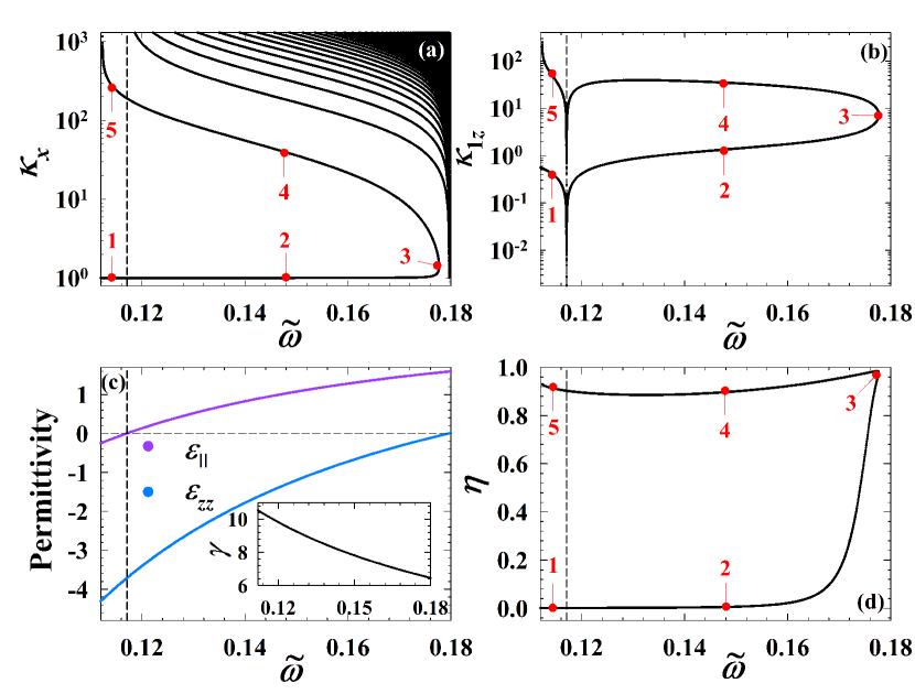
Figure 2: Diagrams depicting the scaled frequency dependence to the relevant physical quantities for the Weyl semimetal waveguide shown in Fig. 1. (a) The mode diagram showing the dimensionless propagation constant $\kappa_{x}$. The numbers $1\rightarrow 5$ identify regions of the diagram discussed below. (b) The normalized wavevector in the WS region $\kappa_{1z}$ for the labeled band in (a). (c) The frequency dependence of the diagonal permittivity components $\epsilon_{\parallel}$ and $\epsilon_{zz}$ are shown in the main plot while the off-diagonal component $\gamma$ is shown in the inset. (d) The energy confinement factor $\eta$ for the modes calculated in (a). Note that $\kappa_{x}$ and $\kappa_{1z}$ are shown on a logarithmic scale. The modes to the left of the vertical line in panel (a) correspond to the frequency range in which $\epsilon_{\parallel}$ and $\epsilon_{zz}$ are both negative [see panel (c)]. The dimensionless WS material parameters are set to $\beta=0.9$ and $\widetilde{\mu}=0.2$.

In Fig. 2(a), we present the dispersion diagram in terms of the dimensionless propagation constant $\kappa_{x}$ and frequency $\widetilde{\omega}$. Various points are numerically labeled on the diagram for discussion below. We consider subwavelength widths corresponding to $k_{c}d=0.03$, where $k_{c}$ is a characteristic wavenumber corresponding to $k_{c}=\omega_{c}/c$, at the normalized design frequency $\widetilde{\omega}_{c}=0.12$. The conical tilt is fixed at $\beta=0.9$. As seen, there are a discrete number of bands, which arise from the geometrical constraint placed upon the fields from the bounding surfaces. Also, since the fields in the vacuum decay over the length scale $k^{-1}_{0}$, regions of the dispersion curves near the light line ($\kappa_{x}\sim 1$) correspond to a larger decay length, and thus the fields reside mainly outside the guiding layer. The curves that lie to the left of the vertical dashed line identify modal solutions that are predominately evanescent, with the EM field decaying on both sides of the WS/vacuum interface. This arises when both $\epsilon_{\parallel}$ and $\epsilon_{zz}$ are negative. For frequencies to the right of the vertical line, the modes transition from predominately evanescent in the WS, to sinusoidal, whereby $\epsilon_{\parallel}>0$ and $\epsilon_{zz}<0$. The modes at these frequencies of course still decay in the vacuum region. In Fig. 2(b), the normalized wavevector in the WS, $\kappa_{1z}$, is shown. Due to the decoupling of the TE and TM modes, we have $\kappa_{\pm}\rightarrow\kappa_{1z}$. At the transition point between oscillatory and evanescent modes (vertical line at $\widetilde{\omega}\approx 0.117$), $\epsilon_{\parallel}\approx 0$, and consequently the wavevector drastically diminishes, corresponding to a very long wavelength in the WS. On the other hand, when $\epsilon_{zz}\approx 0$ (point 3), the wavevector is noticeably larger. The correlations between the mode diagrams and the EM response is shown in Fig. 2(c). Notably, $\epsilon_{\parallel}$ and $\epsilon_{zz}$ become vanishingly small at different frequencies, leading to an interesting anisotropic ENZ response. In particular, at the crossover point $\widetilde{\omega}\approx 0.117$, $\epsilon_{\parallel}\approx 0$, and $\epsilon_{zz}<0$. Indeed, when the energies associated with the chemical potential and frequency are similar, $\epsilon_{\parallel}\approx 0$ when $\omega\approx 2\mu/\sqrt{3\pi/\alpha+\log(4\Gamma^{2}/(3\mu^{2}))}$. The other ENZ scenario occurs at the higher frequency $\widetilde{\omega}\approx 0.18$, where $\epsilon_{zz}\approx 0$, and $\epsilon_{\parallel}>0$. This is also in the vicinity where the slope of the dispersion curve in Fig. 2(a) changes sign (labeled 3). This feature of the dispersion diagram corresponds to where $\kappa_{x}$ close to the light line bends back and rapidly increases. Similar behavior is seen in general, when a waveguide is in contact with another medium possessing permittivity components that are opposite in sign. The corresponding energy flow along the interface that separates the two media undergoes an abrupt reversal when going from vacuum to the WS or vice versa. Additionally, extreme field enhancement can occur when either of the permittivity components is near the ENZ regime. For example, since the boundary conditions dictate that the ratio of the normal components of the electric fields at the semimetal interface are $E_{z1}/E_{z0}\sim 1/\epsilon_{zz}$, a substantial mismatch in field strengths can clearly occur when $\epsilon_{zz}\sim 0$. Although its effects are weak for a subwavelength WS, for completeness the inset presents the frequency dependence to the off-diagonal component $\gamma$ calculated via the methods described in the Appendix. Lastly, in Fig. 2(d), the energy confinement factor $\eta$ is shown as a function of normalized frequency. The labeled numbers identify the corresponding ($\kappa_{x}$, $\widetilde{\omega}$) pairs in Fig. 2(a). The fraction of time-averaged EM energy within the WS at frequency points 1 and 2 is shown to be extremely small due to the fact that modes with $\kappa_{x}\sim 1$ correspond to the EM fields residing mainly in the vacuum region. The upper branch at points $3\rightarrow 5$ reveals that a substantial percentage of the energy density is contained within the semimetal. We see that $\eta$ is maximal at position 3, where the slope of the dispersion diagram changes sign [see Fig. 2(a)], and $\epsilon_{zz}\approx 0$, giving rise to a large increase of the electric field normal to the interface.

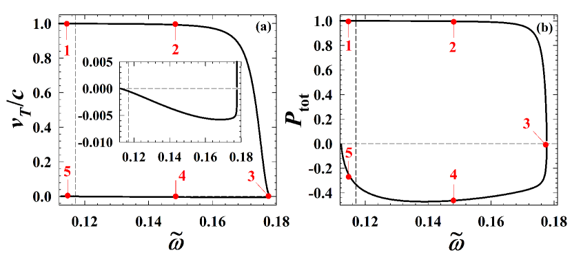
Figure 3: (a) The energy transport velocity (normalized by the speed of light $c$) as a function of dimensionless frequency. The inset is a magnification of $v_{T}$ for the lower curve along the points $3\rightarrow 5$. (b) The total normalized power of the system. Both $v_{T}$ and $P_{\rm tot}$ are calculated for the modes described by the first dispersion curve in Fig. 2(a), and correlated with the number labels. The WS has its conical tilting parameter set to $\beta=0.9$.

To gain additional perspectives on the energy flow in the system, we present in Fig. 3(a), the energy transport velocity $v_{T}$ as a function of the normalized frequency. To calculate this quantity we take the ratio of the Poynting vector to the energy density per Eq. (28). For the subwavelength structure under consideration, the time-averaged energy density can be calculated approximately for the WS region:

$$U_{1}\approx\frac{\mu(\kappa_{x}^{2}-1)}{4(\epsilon_{zz}-\kappa_{x}^{2})^{2}\sin^{2}(k_{+}d)}\bigg{\{}(\epsilon_{zz}^{2} +\frac{\partial(\omega\epsilon_{zz})}{\partial\omega}\kappa_{x}^{2})\kappa_{+}^{2}\cos^{2}(k_{+}d[1+\frac{z}{d}])$$

$$+\frac{\partial(\omega\epsilon_{\parallel})}{\partial\omega}(\epsilon_{zz}-\kappa_{x}^{2})^{2}\sin^{2}(k_{+}d[1+\frac{z}{d}])\bigg{\}},$$ (29)

while for the vacuum region, we have:

$$U_{0}=\frac{\mu\kappa_{x}^{2}}{2}e^{-2k_{0}z\sqrt{\kappa_{x}^{2}-1}}.$$ (30)

Likewise, the time-averaged Poynting vector component $S_{x}$ (for $d/\lambda\ll 1$) can be expressed as,

$$S_{x1}\approx\frac{c\mu\epsilon_{zz}\kappa_{x}(\kappa_{x}^{2}-1)\kappa_{+}^{2}\cos^{2}(k_{+}d[1+z/d])}{2(\epsilon_{zz}-\kappa_{x}^{2})^{2}\sin^{2}(k_{+}d)},$$ (31)

and for the vacuum region:

$$S_{x0}=\frac{c\mu\kappa_{x}}{2}e^{-2k_{0}z\sqrt{\kappa_{x}^{2}-1}}.$$ (32)

In the absence of loss, the energy transport direction lies solely along the interface ($x$-direction), so that ${\bm{v}}_{T}=v_{T}\hat{\bm{x}}$. Note that when $\kappa_{x}\rightarrow 1$, $v_{T}$ corresponds to the expected phase velocity, or velocity at which plane wavefronts travel along the $x$-direction: $v_{T}={c}/{\kappa_{x}}$. It is evident from Fig. 3(a), that $v_{T}$ obeys casualty, with $v_{T}\leq c$. Due in part to the competing effects that can arise in structures with counter-propagating energy flows on opposite sides of the waveguide interface, the transport of energy can occur at effective speeds smaller than $c$. In particular, it is evident that $v_{T}$ can become very small for the modes labeled $3\rightarrow 5$. Note that from the inset, we see that over the entire frequency range, $v_{T}$ is slightly negative, but never zero until at the crossover point (3), where the dispersion curve in Fig. 2(a) changes direction. For modes 1 and 2, where $\kappa_{x}\approx 1$, a large portion of the EM field resides in the vacuum region, and thus the net transport of energy has $v_{T}/c\approx 1$. Slow-light phenomena have been explored previously [63, 64] in ENZ and metamaterial systems. The flow of energy involves both the interplay between the propagating and stored forms of energy. The proposed WS waveguide thus serves as an effective platform for studying slow-energy effects in dissipationless systems, where the energy propagation in adjacent regions are oppositely directed due to the sign change of the permittivity across the interface. Having tunable control over the speed of energy transport can also have practical uses in optical memory devices, biosensing [65], and chemical sensors [66].

As a complimentary study, we show in Fig. 3(b), the total power $P_{\rm tot}$ of the system, where we define,

$$P_{\rm tot}=\frac{P_{x0}+P_{x1}}{|P_{x0}|+|P_{x1}|}.$$ (33)

The upper branch of the power curve at unity (modes $1\rightarrow 2$) corresponds to the dispersion curve where $\kappa_{x}\sim 1$ in Fig. 2(a), where the energy flows predominately outside the semimetal. The net power drops drastically to zero at the transition point (mode 3), where the slope of the dispersion curve changes sign. This follows from the superposition of two counter-propagating energy flows, and is consistent with the behavior of the group velocity $v_{g}\equiv\partial\omega/\partial k_{x}$, which becomes vanishingly small at point 3. Reducing the frequency, and going from points $3\rightarrow 5$, it is apparent that the power reverses and now has a net flow in the opposite (negative) direction, corresponding to the upper branch of the dispersion curve in Fig. 2(a), until the net power again vanishes at $\widetilde{\omega}\approx 0.112$.

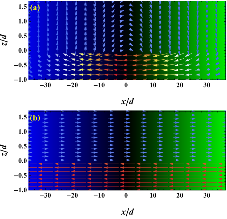
Figure 4: (a) Representative snapshot of the instantaneous Poynting vector ${\bm{E}}\times{\bm{H}}$. (b) The time-averaged Poynting vector, averaged over one cycle. The frequency in both cases corresponds to the point on the dispersion diagram in Fig. 3(a) where the energy velocity vanishes (labeled 3). The interface between the vacuum region and the WS is located at $z=0$.

As alluded to earlier, for frequencies in which the diagonal permittivity components change sign when crossing into another medium, the resultant flow of energy in each region can often times be oppositely directed. To visualize the directional dependence to the energy flow, we present in Fig. 4, the spatial behavior of the Poynting vector in the surrounding vacuum region ($z/d>0$), and within the WS ($0\leq z/d\leq-1$). We consider the frequency and propagation constant corresponding to point 3 on the dispersion curve in Fig. 2(a). At this point $\epsilon_{zz}$ is slightly negative, with $\epsilon_{zz}\approx 0$, and $\epsilon_{\parallel}\approx 1$. First, in Fig. 4(a), the instantaneous Poynting vector is shown. We see that the energy flow tends to form a vortex-like pattern in which the flow of energy upward is counteracted by the flow downward. Since the normal component of the ${\bm{E}}$ field is discontinuous at the interface, the energy flow undergoes an abrupt change at $z=0$. Since there is no dissipation however, when averaging over a complete period, there is no net power flow in the $z$ direction. This is seen in Fig. 2(b), where the time-averaged Poynting vector is presented. The cancellation of the energy flow normal to the interface leads to a net propagation of energy only along the interface ($x$ direction). We saw earlier in Fig. 3(b) that this mode corresponds to a vanishing net power flow. Thus, the spatially integrated Poynting vector component along the interface in each region completely cancel one another, leading to a net effective energy velocity of zero [see Fig. 3(a)].

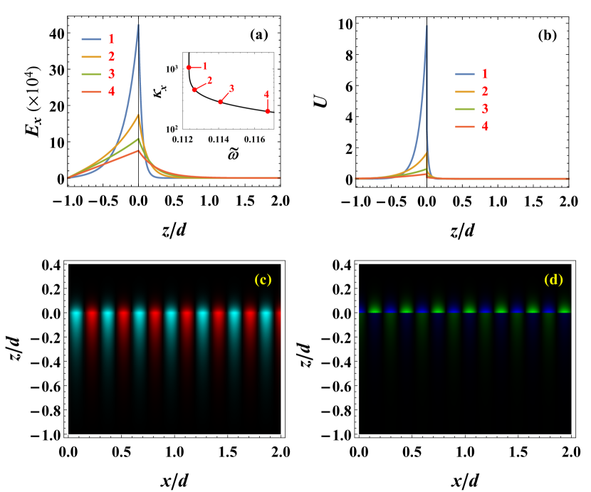
Figure 5: Spatial behavior of the electromagnetic field profiles. (a) The $x$-component of the electric field $E_{x}$ is plotted as a function of the normalized coordinate $z/d$. In (b) the electromagnetic energy density $U$ is shown. The legends in (a) and (b) identify the four frequencies considered along the dispersion curve shown in the inset. As the frequency increases, the overall field amplitudes are shown to decline. The vertical line at $z=0$ locates the vacuum/WS interface. Panels (c) and (d) are color maps depicting $E_{x}$ and $E_{z}$, respectively. Bright regions correspond to high field intensities. The frequency corresponds to the mode labeled 1 in panel (a), and the tilt parameter is set to $\beta=0.9$.

We now turn our attention to the explicit behavior of the fields themselves. In Fig. 5(a) we show the spatial behavior of the electric field parallel to the interface $E_{x}$. Four representative frequencies are considered along the dispersion curve show in the inset. These modes correspond to the regime that is left of the vertical dashed line in Fig. 2(a), and thus these modes are strictly evanescent on both sides of the interface. It is noted that as the frequency approaches the lowest frequency case, $\widetilde{\omega}\approx 0.112$ (labeled 1), the electric field becomes strongly enhanced. As was observed in Fig. 3, this correlates with the frequency in which $v_{T}\approx 0$, and the slope of the dispersion curve vanishes. Note that over the considered frequency range, both diagonal components of $\overline{\overline{\epsilon}}$ are negative, and $\epsilon_{\parallel}\approx 0$. Thus, these are purely evanescent modes with field profiles that decay on both sides of the vacuum/WS interface, as is clearly seen in Fig. 2(a). The energy density, which contains both the electric and magnetic fields also exhibits strong field localization at the interface as seen Fig. 2(b). Next in Figs. 5(c) and 5(d), color maps illustrate the full spatial profiles the tangential ($E_{x}$) and normal ($E_{z}$) electric field components, respectively. Here the propagating term $e^{ik_{x}x}$ is included for all field components. The tilt parameter $\beta$ is set to $\beta=0.9$, while $\widetilde{\omega}$ is fixed to the frequency labeled 1 in the mode diagram shown in the inset of Fig. 5(a). It is evident from Figs. 5(c) and 5(d) that the propagating electric field has both field polarizations strongly confined to the interface. As shown in Figs. 5(a) and 5(b), the EM fields also become substantially enhanced at this frequency.

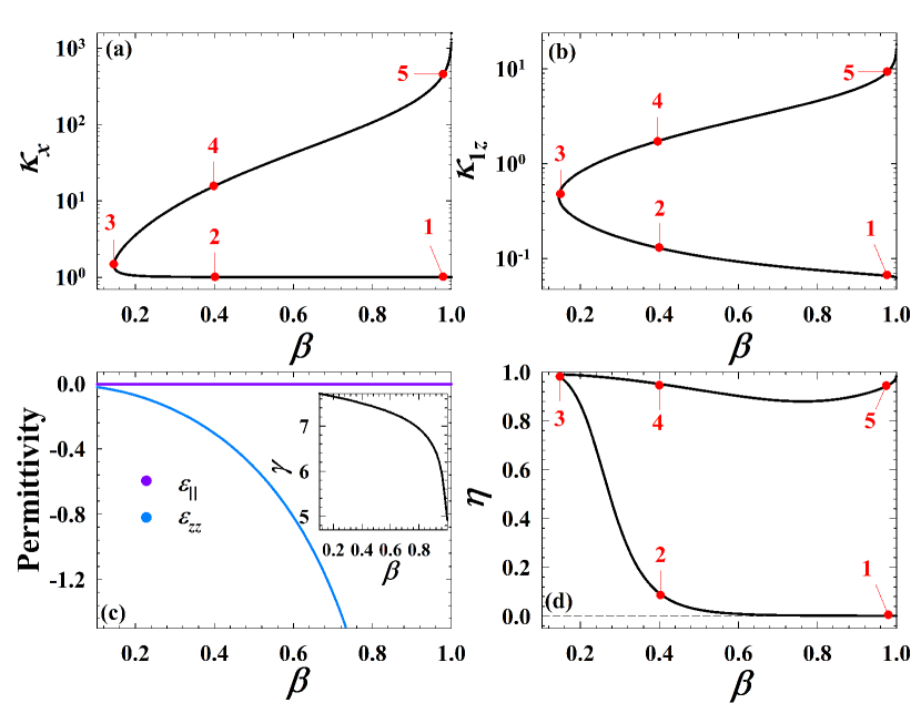
Figure 6: The effects of the conical tilt $\beta$ on the waveguide characteristics. In (a) the propagation constant $\kappa_{x}$ is shown vs $\beta$. The wavevector in the WS, $\kappa_{1z}$, is shown in (b). The electromagnetic response of the WS waveguide is shown in (c), where the diagonal components of the permittivity tensor $\epsilon_{\parallel}$ and $\epsilon_{zz}$ are presented in the main plot, while the inset reveals the off-diagonal component $\gamma$. The fraction of EM energy $\eta$ that is confined to the semimetal for the modes calculated in (a) is shown in (d). The normalized frequency corresponds to $\widetilde{\omega}=0.117$, which is the point labeled 5 of the dispersion curve shown in Fig. 2(a). Note that $\kappa_{x}$ and $\kappa_{1z}$ are shown on a logarithmic scale.

We now discuss how the tilt of the Weyl cones directly influences the mode diagrams and corresponding EM field characteristics. In Fig. 6(a), the dimensionless propagation constant $\kappa_{x}$ is shown as a function of tilt $\beta$. For clarity of discussion later, the numbers label relevant parts of the dispersion diagram. In Fig. 6(b) the wavevector in the WS, $\kappa_{1z}$ is also shown over a wide range of $\beta$. In contrast to what was observed in Fig. 2(b) when varying the frequency, here the wavevector in the WS monotonically increases along the dispersion path $1\rightarrow 5$. In Fig. 6(c) the EM response of both the diagonal (main plot) and off-diagonal (inset) components of $\overline{\overline{\epsilon}}$ is shown over the same range of $\beta$. For the given frequency, $\widetilde{\omega}=0.117$, both components $\epsilon_{\parallel}$ and $\epsilon_{zz}$ are negative, with $\epsilon_{\parallel}\approx 0$. Examining Fig. 6(a), we see that the main dispersion curve has the lower branch with points $1\rightarrow 3$ close to the light line. The upper branch from $3\rightarrow 5$ is associated with substantially larger propagation constants that increase rapidly with tilt. The corresponding confinement factor is presented in Fig. 6(c). As expected, the fraction of energy $\eta$ contained in the WS is very small for points $1$ and $2$, where $\kappa_{x}\rightarrow 1$, reflecting the predominance of the energy density outside of the guiding semimetal layer. There is a significant fraction of the energy density in the WS for modes occupying the upper dispersion curve along the path $3\rightarrow 5$. Moreover, $\eta\rightarrow 1$ for conical tilts in the vicinity of points 3 and 5, where $\partial\beta/\partial\kappa_{x}\rightarrow 0$ in Fig. 6(a). Thus, we see that the tilt of the Weyl cones plays an important role in determining the propagation and spatial localization properties for guided wave modes.

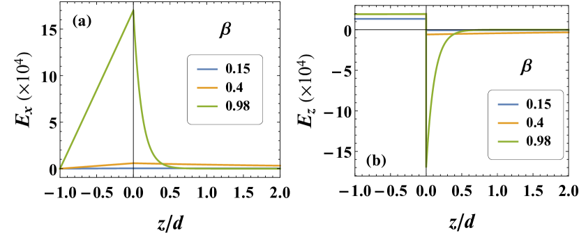
Figure 7: Panels (a) and (b) display the electric field profiles as a function of the normalized position $z/d$. The legends depict the range of conical tilts considered, which correspond to the upper branch of the mode diagram in Fig. 6(a) (with the labels $3\rightarrow 5$). The frequency is identical to that used in Fig. 6.

To study the guided modes in the ENZ regime further, we keep the wave frequency the same as in Fig. 6, corresponding to where $\epsilon_{\parallel}\approx 0$, and investigate the spatial behavior of the fields. Thus, in Fig. 7, the components of the electric field $E_{x}$ and $E_{z}$ are shown as a function of the scaled coordinate $z/d$ for varying tilt of the Weyl cones. The three values of the tilt parameter shown in the legend corresponds to the points $3\rightarrow 5$ of the mode diagram in Fig. 6(a). Notably, there is a linear variation in $E_{x}$, while $E_{z}$ is constant throughout the WS layer. The ${\bm{E}}$-field for both components then decays once entering the vacuum region, as is required for guided waves. For both components, increasing the tilt results in a field enhancement, as $\epsilon_{zz}$ becomes increasingly more negative, resulting in modes with larger $\kappa_{x}$ [see upper branch of Fig. 6(a)]. To understand this overall behavior explicitly, we write the general expressions for the EM fields and then take the limit $\epsilon_{\parallel}\rightarrow 0$, arriving at:

$$E_{x1} \approx iZ_{0}\sqrt{\kappa_{x}^{2}-1}\left(1+\frac{z}{d}\right),$$ (34)

$$E_{z1} \approx\frac{Z_{0}\kappa_{x}\sqrt{\kappa_{x}^{2}-1}}{k_{0}d(\kappa_{x}^{2}-\epsilon_{zz})},$$ (35)

$$H_{y1} \approx\frac{\epsilon_{zz}\sqrt{\kappa_{x}^{2}-1}}{k_{0}d(\epsilon_{zz}-\kappa_{x}^{2})},$$ (36)

where the factor $e^{ik_{x}x}$ has been suppressed. The linear dependence seen in Fig. 7 for $E_{x1}$ is clearly evident from Eq. (34), while the spatial dependence in $E_{z1}$ and $H_{y1}$ drops out, leading to the uniform component of the electric field normal to the interface, seen in Fig. 7(b). Interestingly, despite the fact that $E_{z1}$ is a function of $\kappa_{x}$ and $\epsilon_{zz}$, both of which depend strongly on $\beta$ [see Fig. 6(a) and 6(c)], they tend to counteract one another, leading to the weak $\beta$ dependence observed for $E_{z1}$ in Fig. 7(b). It is instructive to also examine the energy flow via the Poynting vector. Within the ENZ regime, we find,

$$S_{x1}\approx\frac{Z_{0}}{2}\frac{\epsilon_{zz}\kappa_{x}(\kappa_{x}^{2}-1)}{(k_{0}d)^{2}(\epsilon_{zz}-\kappa_{x}^{2})^{2}},$$ (37)

which is independent of position in the WS. The spatially averaged energy density in the WS is,

$$\langle U_{1}\rangle\approx\mu(\kappa_{x}^{2}-1)\frac{\omega\partial_{\omega}(\epsilon_{\parallel})(k_{0}d)^{2}(\epsilon_{zz}-\kappa_{x}^{2})^{2}+3(\epsilon_{zz}^{2}+\kappa_{x}^{2}\partial_{\omega}(\omega\epsilon_{zz}))}{12(k_{0}d)^{2}(\epsilon_{zz}-\kappa_{x}^{2})^{2}}.$$ (38)

To obtain the speed of EM energy transport, it is then a simple matter to take the corresponding ratio via Eq. (28). The dispersion diagram can also be found analytically in the ENZ regime. When $\epsilon_{\parallel}\approx 0$, the propagation constant can be written:

$$\kappa_{x}\approx\frac{\sqrt{\epsilon_{zz}[\epsilon_{zz}+2(k_{0}d)^{2}\pm\sqrt{\epsilon^{2}_{zz}+(2k_{0}d)^{2}(\epsilon_{zz}-1)}}]}{\sqrt{2}k_{0}d},$$ (39)

which is a convenient expression that negates the need to numerically solve a transcendental equation for the dispersion diagram.

3 Conclusions

We have analyzed the dispersion diagrams and electromagnetic field behavior of a subwavelength planar Weyl semimetal waveguide system where the Dirac cones in the touching points of valance and conduction bands possess the possibility to be tilted. We found that the electromagnetic response for each diagonal component of the permittivity tensor can be made is vanishingly small, creating an anisotropic epsilon-near-zero configuration. The admitted waveguide modes were presented in the form of dispersion diagrams, where regimes of high energy-density confinement in the Weyl semimetal layer were found. We also showed how the net system power can be manipulated to vanish at critical points of the dispersion curves, where the propagation velocity of electromagnetic energy is zero. Our results offer waveguides made of Weyl semimetals with controllable energy flow velocity and direction by materials and geometrical parameters.

Funding

K.H. is supported in part by ONR and a grant of HPC resources from the DOD HPCMP. M.A. is supported by Iran’s National Elites Foundation (INEF).

Disclosures

The authors declare that there are no conflicts of interest related to this article.

Appendix A Calculation of $\gamma$: the off-diagonal component of the permittivity tensor $\overline{\overline{\epsilon}}$

When calculating the off-diagonal component $\gamma$ for arbitrary parameters, it is convenient to separate Fermi surface and vacuum contributions to $\gamma(\omega)=\sum_{s=\pm}[\gamma^{(s)}_{FS}(\omega)+\gamma^{(s)}_{0}(\omega)]$, where

$$\gamma^{(s)}_{FS}(\omega) =\frac{s\alpha}{\omega^{2}}\int_{0}^{\infty}\frac{p_{\perp}dp_{\perp}}{2\pi}\int_{-\Gamma-sv_{F}Q}^{\Gamma-sv_{F}Q}dp_{z}\frac{p_{z}}{p}\frac{i\omega_{k}}{p^{2}+\omega_{k}^{2}/4}[\Theta(\mu-\zeta_{s,+})-\Theta(\mu-\zeta_{s,-})-1],$$ (40)

and

$$\gamma^{(s)}_{0}(\omega)=\frac{s\alpha}{\omega^{2}}\int_{0}^{\infty}\frac{p_{\perp}dp_{\perp}}{2\pi}\int_{-\Gamma_{0}-sv_{F}Q}^{\Gamma_{0}-sv_{F}Q}dp_{z}\frac{p_{z}}{p}\frac{i\omega_{k}}{p^{2}+\omega_{k}^{2}/4},$$ (41)

where the following limit is taken in the integrals: $\omega_{k}\rightarrow\omega+i\delta$. This ensures proper convergence when numerically evaluating Eqs. (40)-(41). We have also defined $\zeta_{s,t}\equiv tp+p_{z}\beta_{s}$, $p=\sqrt{p_{z}^{2}+p_{\perp}^{2}}$, and a momentum cutoff along the $z$ axis, $\Gamma$. Generally, the cut-off $\Gamma$ is a function of the tilt parameter. Nevertheless, in our calculations, we choose a large enough cut-off and neglect the contribution of $\beta$ to $\Gamma$. The cut-off $\Gamma_{0}>v_{F}|Q|$ is introduced for the correct definition of the vacuum contribution.

Appendix B Details of the coefficients

Without loss of generality, we choose our EM field normalizations so that $r_{1}$=1. After matching the tangential electric and magnetic fields at the air/WS interface, and using the PEC boundary conditions, some straightforward algebra gives the $r_{2}$ coefficient:

$$r_{2}=\frac{\kappa_{x}\gamma[\epsilon_{zz}\kappa_{0z}\kappa_{-}\kappa_{+}(\cos q_{-}-\cos q_{+})+(\kappa_{x}^{2}-\epsilon_{zz})(\kappa_{+}\sin q_{-}-\kappa_{-}\sin q_{+})]}{\epsilon_{zz}[\kappa_{+}(\kappa_{x}^{2}+\kappa_{+}^{2}-\epsilon_{\parallel})(\kappa_{-}\cos q_{-}+\kappa_{0z}\sin q_{-})-\kappa_{-}(\kappa_{x}^{2}+\kappa_{-}^{2}-\epsilon_{\parallel})(\kappa_{+}\cos q_{+}+\kappa_{0z}\sin q_{+})]},$$ (42)

and,

$$a_{1} =Z_{0}\frac{r_{2}\epsilon_{zz}(\epsilon_{\parallel}-\kappa_{x}^{2}-\kappa_{-}^{2})(i\kappa_{0z}+\kappa_{+})+\kappa_{x}\gamma(i(\kappa_{x}^{2}-\epsilon_{zz})+\epsilon_{zz}\kappa_{0z}\kappa_{+})}{2\epsilon_{zz}\kappa_{x}\kappa_{+}(\kappa_{+}^{2}-\kappa_{-}^{2})},$$ (43)

$$b_{1} =Z_{0}\frac{r_{2}\epsilon_{zz}(\epsilon_{\parallel}-\kappa_{x}^{2}-\kappa_{-}^{2})(\kappa_{+}-i\kappa_{0z})+\kappa_{x}\gamma(i(\epsilon_{zz}-\kappa_{x}^{2})+\epsilon_{zz}\kappa_{0z}\kappa_{+})}{2\epsilon_{zz}\kappa_{x}\kappa_{+}(\kappa_{+}^{2}-\kappa_{-}^{2})},$$ (44)

$$c_{1} =Z_{0}\frac{r_{2}\epsilon_{zz}(\epsilon_{\parallel}-\kappa_{x}^{2}-\kappa_{+}^{2})(i\kappa_{0z}+\kappa_{-})+\kappa_{x}\gamma(i(\kappa_{x}^{2}-\epsilon_{zz})+\epsilon_{zz}\kappa_{0z}\kappa_{-})}{2\epsilon_{zz}\kappa_{x}\kappa_{-}(\kappa_{-}^{2}-\kappa_{+}^{2})},$$ (45)

$$d_{1} =Z_{0}\frac{r_{2}\epsilon_{zz}(\epsilon_{\parallel}-\kappa_{x}^{2}-\kappa_{+}^{2})(\kappa_{-}-i\kappa_{0z})+\kappa_{x}\gamma(i(\epsilon_{zz}-\kappa_{x}^{2})+\epsilon_{zz}\kappa_{0z}\kappa_{-})}{2\epsilon_{zz}\kappa_{x}\kappa_{-}(\kappa_{-}^{2}-\kappa_{+}^{2})}.$$ (46)

Once the dispersion equation [Eq. (2.2)] is solved for the propagation constant $\kappa_{x}$, the coefficients above can be determined to construct the EM fields.

References

- [1] H.Z. Weyl, Elektron und Gravitation. I, Physik 56, 330 (1929).
- [2] M. Z. Hasan and C. L. Kane, Colloquium: Topological insulators, Rev. Mod. Phys. 82, 3045 (2010).
- [3] X.-L. Qi and S.-C. Zhang, Topological insulators and superconductors, Rev. Mod. Phys. 83, 1057 (2011).
- [4] A. A. Burkov and L. Balents, Weyl semimetal in a topological insulator multilayer, Phys. Rev. Lett. 107, 127205 (2011).
- [5] X. Wan, A. M. Turner, A. Vishwanath, and S. Y. Savrasov, Topological semimetal and Fermi-arc surface states in the electronic structure of pyrochlore iridates, Phys. Rev. B 83, 205101 (2011).
- [6] Z. Wang, Y. Sun, X.-Q. Chen, C. Franchini, G. Xu, H. Weng, X. Dai, and Z. Fang, Dirac semimetal and topological phase transitions in Bi (, K, Rb), Phys. Rev. B 85, 195320 (2012).
- [7] S.-M. Huang, S.-Y. Xu, I. Belopolski, C.-C. Lee, G. Chang, B. Wang, N. Alidoust, G. Bian, M. Neupane, C. Zhang, S. Jia, A. Bansil, H. Lin, and M. Z. Hasan, A Weyl Fermion semimetal with surface Fermi arcs in the transition metal monopnictide TaAs class, Nat. Commun. 6, 7373 (2015).
- [8] H. Weng, C. Fang, Z. Fang, B. A. Bernevig, and X. Dai, Weyl semimetal phase in noncentrosymmetric transition-metal monophosphides, Phys. Rev. X 5, 011029 (2015).
- [9] C. Shekhar, A. K. Nayak, Y. Sun, M. Schmidt, M. Nicklas, I. Leermakers, U. Zeitler, Y. Skourski, J. Wosnitza, Z. Liu, Y. Chen, W. Schnelle, H. Borrmann, Y. Grin, C. Felser, and B. Yan, Extremely large magnetoresistance and ultrahigh mobility in the topological Weyl semimetal candidate NbP, Nat. Phys. 11, 645 (2015).
- [10] I. Belopolski, S.-Y. Xu, Y. Ishida, X. Pan, P. Yu, D. S. Sanchez, M. Neupane, N. Alidoust, G. Chang, T.-R. Chang, Y. Wu, G. Bian, H. Zheng, S.-M. Huang, C.-C. Lee, D. Mou, L. Huang, Y. Song, B. Wang, G. Wang, Y.-W. Yeh, N. Yao, J. Rault, P. Lefevre, F. Bertran, H.-T. Jeng, T. Kondo, A. Kaminski, H. Lin, Z. Liu, F. Song, S. Shin, and M. Z. Hasan, Unoccupied electronic structure and signatures of topological Fermi arcs in the Weyl semimetal candidate , arXiv:1512.09099 (2015).
- [11] S.-Y. Xu, I. Belopolski, N. Alidoust, M. Neupane, G. Bian, C. Zhang, R. Sankar, G. Chang, Z. Yuan, C.-C. Lee, S.-M. Huang, H. Zheng, J. Ma, D. S. Sanchez, B. Wang, A. Bansil, F. Chou, P. P. Shibayev, H. Lin, S. Jia, and M. Z. Hasan, Discovery of a Weyl fermion semimetal and topological Fermi arcs, Science 349, 613 (2015).
- [12] S.-Y. Xu, N. Alidoust, I. Belopolski, Z. Yuan, G. Bian, T.-R. Chang, H. Zheng, V. N. Strocov, D.S. Sanchez, G. Chang, C. Zhang, D. Mou, Y. Wu, L. Huang, C.-C. Lee, S.-M. Huang, B. Wang, A. Bansil, H.-T. Jeng, T. Neupert, A. Kaminski, H. Lin, S. Jia, and M.Z. Hasan, Discovery of a Weyl fermion state with Fermi arcs in niobium arsenide, Nat. Phys. 11, 748 (2015).
- [13] B. Q. Lv, H. M. Weng, B. B. Fu, X. P. Wang, H. Miao, J. Ma, P. Richard, X. C. Huang, L. X. Zhao, G. F. Chen, Z. Fang, X. Dai, T. Qian, and H. Ding, Experimental Discovery of Weyl Semimetal TaAs, Phys. Rev. X 5, 031013 (2015).
- [14] Y. Sun, S.-C. Wu, M. N. Ali, C. Felser, B. Yan, Prediction of Weyl semimetal in orthorhombic MoTe2, Phys. Rev. B 92, 161107 (2015).
- [15] G. Autès, D. Gresch, M. Troyer, A.A. Soluyanov, and O.V. Yazyev, Robust Type-II Weyl Semimetal Phase in Transition Metal Diphosphides X ( = ), Phys. Rev. Lett. 117, 066402 (2016).
- [16] Y. Wu, N. Hyun Jo, D. Mou, L. Huang, S. L. Bud’ko, P. C. Canfield, A. Kaminski, Observation of Fermi arcs in the type-II Weyl semimetal candidate , Phys. Rev. B 94, 121113(R) (2016).
- [17] S.-Y. Xu, N. Alidoust, G. Chang, H. Lu, B. Singh, I. Belopolski, D. S. Sanchez, X. Zhang, G. Bian, M.-A. Husanu, Y. Bian, S.-M. Huang, C.-H. Hsu, T.-R. Chang, H.-T. Jeng, A. Bansil, T. Neupert, V. N. Strocov, H. Lin, S. Jia, and M. Z. Hasan, Discovery of Lorentz-violating type II Weyl fermions in LaAlGe, Science Advances 3, e1603266 (2017).
- [18] E. Haubold, K. Koepernik, D. Efremov, S. Khim, A. Fedorov, Y. Kushnirenko, J. van den Brink, S. Wurmehl, B. Buchner, T. K.Kim, M. Hoesch, K. Sumida, K. Taguchi, T. Yoshikawa, A. Kimura, T. Okuda, S. V. Borisenko, Experimental realization of type-II Weyl state in noncentrosymmetric , Phys. Rev. B 95, 241108(R) (2017).
- [19] M. A. Kats, D. Sharma, J. Lin, P. Genevet, R. Blanchard, Z. Yang, M. M. Qazilbash, D. N. Basov, S. Ramanathan, and F. Capasso, Imaginary part of Hall conductivity in a tilted doped Weyl semimetal with both broken time-reversal and inversion symmetry, Appl. Phys. Lett. 101, 221101 (2012).
- [20] T. Timusk, J. P. Carbotte, C. C. Homes, D. N. Basov, and S. G. Sharapov, Three-dimensional Dirac fermions in quasicrystals as seen via optical conductivity, Phys. Rev. B 87, 235121 (2013).
- [21] P.E.C. Ashby and J. P. Carbotte, Magneto-optical conductivity of Weyl semimetals, Phys. Rev. B 87, 245131 (2013).
- [22] P.E.C. Ashby and J. P. Carbotte, Chiral anomaly and optical absorption in Weyl semimetals, Phys. Rev. B 89 245121 (2014).
- [23] M. Kargarian, M. Randeria, and N. Trivedi, Theory of Kerr and Faraday rotations and linear dichroism in Topological Weyl Semimetals, Sci. Rep. 5, 12683 (2015).
- [24] A.A. Zyuzin and V.A. Zyuzin, Chiral electromagnetic waves in Weyl semimetals, Phys. Rev. B 92, 115310 (2015).
- [25] R. Y. Chen, S. J. Zhang, J. A. Schneeloch, C. Zhang, Q. Li, G. D. Gu, and N. L. Wang, Optical spectroscopy study of the three-dimensional Dirac semimetal , Phys. Rev. B 92, 075107 (2015).
- [26] A. B. Sushkov, J. B. Hofmann, G. S. Jenkins, J. Ishikawa, S. Nakatsuji, S. Das Sarma, and H. D. Drew, Optical evidence for a Weyl semimetal state in pyrochlore , Phys. Rev. B 92, 241108 (2015).
- [27] O. V. Kotov and Yu. E. Lozovik, Dielectric response and novel electromagnetic modes in three-dimensional Dirac semimetal films, Phys. Rev. B 93, 235417 (2016).
- [28] B. Xu, Y. M. Dai, L. X. Zhao, K. Wang, R. Yang, W. Zhang, J. Y. Liu, H. Xiao, G. F. Chen, A. J. Taylor, D. A. Yarotski, R. P. Prasankumar, and X. G. Qiu, Optical spectroscopy of the Weyl semimetal TaAs, Phys. Rev. B 93, 121110 (2016).
- [29] S. P. Mukherjee and J. P. Carbotte, Absorption of circular polarized light in tilted type-I and type-II Weyl semimetals, Phys. Rev. B 96, 085114 (2017).
- [30] Q. Ma, S.-Y. Xu, C.-K. Chan, C.-L. Zhang, G. Chang, Y. Lin, W. Xie, T. Palacios, H. Lin, S. Jia, P. A. Lee, P. J.-Herrero, and N. Gedik, Direct optical detection of Weyl fermion chirality in a topological semimetal, Nat. Physics 13, 842 (2017).
- [31] J. Noh, S. Huang, D. Leykam, Y. D. Chong, K. P. Chen, and M. C. Rechtsman, Experimental observation of optical Weyl points and Fermi arc-like surface states, Nat. Physics 13, 611 (2017).
- [32] F. Detassis, L. Fritz, and S. Grubinskas, Collective effects in tilted Weyl cones: Optical conductivity, polarization, and Coulomb interactions reshaping the cone, Phys. Rev. B 96, 195157 (2017).
- [33] S. P. Mukherjee and J. P. Carbotte, Imaginary part of Hall conductivity in a tilted doped Weyl semimetal with both broken time-reversal and inversion symmetry, Phys. Rev. B 97, 035144 (2018).
- [34] O. V. Kotov and Yu. E. Lozovik, Giant tunable nonreciprocity of light in Weyl semimetals, Phys. Rev. B 98, 195446 (2018).
- [35] T. Tamaya, T. Kato, S. Konabe, and S. Kawabata, Surface plasmon polaritons in thin-film Weyl semimetals, arXiv:1811.08608.
- [36] Q. Chen, A. R. Kutayiah, I. Oladyshkin, M. Tokman, and A. Belyanin, Optical properties and electromagnetic modes of Weyl semimetals, Phys. Rev. B 99, 075137 (2019).
- [37] M. Silveirinha and N. Engheta, Tunneling of Electromagnetic Energy through Subwavelength Channels and Bends using epsilon-Near-Zero Materials, Phys. Rev. Lett. 97, 157403 (2006).
- [38] A. Alù, M. G. Silveirinha, A. Salandrino, and N. Engheta, Epsilon-near-zero metamaterials and electromagnetic sources: Tailoring the radiation phase pattern, Phys. Rev. B 75, 155410 (2007).
- [39] B. Edwards, A. Alù, M. E. Young, M. Silveirinha, and N. Engheta, Experimental verification of epsilon-near-zero metamaterial coupling and energy squeezing using a microwave waveguide, Phys. Rev. Lett. 100, 033903 (2008).
- [40] R. Liu, Q. Cheng, T. Hand, J. J. Mock, T. J. Cui, S. A. Cummer, and D. R. Smith, Experimental demonstration of electromagnetic tunneling through an epsilon-near-zero metamaterial at microwave frequencies, Phys. Rev. Lett. 100, 023903 (2008).
- [41] K. Halterman, S. Feng, and V. C. Nguyen, Controlled leaky wave radiation from anisotropic epsilon near zero metamaterials, Phys. Rev. B 84, 075162 (2011).
- [42] D. Slocum, S. Inampudi, D. C. Adams, S. Vangala, N. A. Kuhta, W. D. Goodhue, V. A. Podolskiy, D. Wasserman, Funneling light through a subwavelength aperture with epsilon-near-zero materials, Phys. Rev. Lett. 107 133901 (2011).
- [43] S. Feng and K. Halterman, Coherent perfect absorption in epsilon-near-zero metamaterials, Phys. Rev. B 86, 165103 (2012).
- [44] V. N. Smolyaninova, B. Yost, K. Zander, M. S. Osofsky, H. Kim, S. Saha, R. L. Greene, I. I. Smolyaninov, Experimental demonstration of superconducting critical temperature increase in electromagnetic metamaterials, Scientific Reports 4, 7321 (2014).
- [45] M. Mattheakis, C. A. Valagiannopoulos, and E. Kaxiras, Epsilon-near-zero behavior from plasmonic Dirac point: Theory and realization using two-dimensional materials, Phys. Rev. B 94, 201404(R) (2016).
- [46] I. Liberal, N. Engheta, Near-zero refractive index photonics, Nat. Photonics 11, 149158 (2017).
- [47] H. Galinski, G. Favraud,, H. Dong, J. S. Totero Gongora, G. Favaro, M. Döbeli, R. Spolenak, A. Fratalocchi and F. Capasso, Scalable, ultra-resistant structural colors based on network metamaterials, Light: Science & Applications 6, e16233 (2017).
- [48] K. Halterman, M. Alidoust, and A. Zyuzin, Epsilon-near-zero response and tunable perfect absorption in Weyl semimetals, Phys. Rev. B 98, 085109 (2018).
- [49] V. Caligiuri, M. Palei , G. Biffi, S. Artyukhin, and R. Krahne, A Semi-Classical View on Epsilon-Near-Zero Resonant Tunneling Modes in Metal/Insulator/Metal Nanocavities, Nano Letters
- [50] A.N. Poddubny, I. Iorsh, P.A. Belov, and Y. Kivshar, Hyperbolic metamaterials, Nat. Photon. 7, 958 (2013).
- [51] G.-D. Xu, T. Pan, T.-C. Zang, and J. Sun, Characteristics of guided waves in indefinite-medium waveguides, Opt. Commun. 281, 2819 (2008).
- [52] Y. He, S. He, and X. Yang, Optical field enhancement in nanoscale slot waveguides of hyperbolic metamaterials, Opt. Lett. 37, 2907 (2012).
- [53] Q. Li, D. E. Kharzeev, C. Zhang, Y. Huang, I. Pletikosic, A. V. Fedorov, R. D. Zhong, J. A. Schneeloch, G. D. Gu, and T. Valla, Chiral magnetic effect in , Nat. Phys. 12, 550 (2016).
- [54] C.-X. Liu, P. Ye, and X.-L. Qi, Chiral gauge field and axial anomaly in a Weyl semimetal, Phys. Rev. B 87, 235306 (2013).
- [55] J. Zhou, H.-R. Chang, and D. Xiao, Plasmon mode as a detection of the chiral anomaly in Weyl semimetals, Phys. Rev. B 91, 035114 (2015).
- [56] D. E. Kharzeev, R. D. Pisarski, and H.-U. Yee, Universality of plasmon excitations in Dirac semimetals, Phys. Rev. Lett. 115, 236402 (2015).
- [57] J. Hofmann and S. Das Sarma, Plasmon signature in Dirac-Weyl liquids, Phys. Rev. B 91, 241108 (2015).
- [58] Qing-Dong Jiang, Hua Jiang, Haiwen Liu, Qing-Feng Sun, and X. C. Xie Topological Imbert-Fedorov Shift in Weyl Semimetals, Phys. Rev. Lett. 115, 156602 (2015).
- [59] D. J. Bergman and Y. M. Strelniker, Anisotropic ac electrical permittivity of a periodic metal-dielectric composite film in a strong magnetic field, Phys. Rev. Lett. 80, 857 (1998).
- [60] K. Halterman and J. M. Elson, Near-perfect absorption in epsilon-near-zero structures with hyperbolic dispersion, Opt. Express 22, 7337 (2014).
- [61] R. Loudon, The propagation of electromagnetic energy through an absorbing dielectric, J. Phys A 3, 233 (1970).
- [62] R. Ruppin, Electromagnetic energy density in a dispersive and absorptive material, Phys. Lett. A 299, 309 (2002).
- [63] A. Ciattoni, A. Marini, C. Rizza, M. Scalora, and F. Biancalana, Polariton excitation in epsilon-near-zero slabs: Transient trapping of slow light, Phys. Rev. A 87, 053853 (2013).
- [64] K. L. Tsakmakidis, A. D. Boardman, and O. Hess, Trapped rainbow storage of light in metamaterials, Nature 450, 397 (2007).
- [65] J. García-Rupérez, V. Toccafondo, M. J. Bañuls, J. G. Castelló, A. Griol, S. Peransi-Llopis, and A. Maquieira, Label-free antibody detection using band edge fringes in SOI planar photonic crystal waveguides in the slow-light regime, Opt. Express 18, 24276 (2010).
- [66] A. Di Falco, L. O’Faolain, T.F. Krauss, Chemical sensing in slotted photonic crystal heterostructure cavities, Appl. Phys. Lett. 94, 063503 (2009).