Bohmian trajectories in an entangled two-qubit system

Abstract

In this paper we examine the evolution of Bohmian trajectories in the presence of quantum entanglement. We study a simple two-qubit system composed of two coherent states and investigate the impact of quantum entanglement on chaotic and ordered trajectories via both numerical and analytical calculations.

1 Introduction

Bohmian Quantum Mechanics (BQM) is one of the main alternative interpretations of Quantum Mechanics (QM) ([1, 2]), where quantum particles follow certain trajectories in spacetime, in sharp contrast with Standard Quantum Mechanics (SQM), where the notion of particle trajectory does not exist. However they both predict the same experimental results. In BQM the usual Schrödinger’s equation (SE) still governs the evolution of the wave function $\Psi$ which in turn guides the particle positions via a set of nonlinear first order in time equations of motion, the Bohmian equations.

Quantum entanglement (QE) is the basic property that makes quantum systems behave differently from classical systems [3], [4]. QE plays a key role in Quantum Information and Computation Theory, since it is useful in many applications such as computing algorithms, quantum teleportation schemes and public key distribution protocols [5]. From a theoretical perspective QE is the manifestation of the non local nature of QM. Consequently it has a central role in Bohmian Mechanics, where it has been studied in different frameworks, such as the theoretical and experimental study of the relation between Bohmian trajectories and quantum measurements [6, 7, 8, 9], the dynamics of interacting many body systems [10], the relation between chaos and entanglement in the case of stationary states (focusing on three-partite systems) [11], the dynamics of dissipative bipartite systems [12] and the study of correlations between spin-1/2 quantum rotors in comparison with SQM [13].

In this paper we investigate the effect of QE on the Bohmian trajectories of a simple system composed of coherent states of two independent harmonic oscillators. Namely we study the Bohmian trajectories on the $x-y$ plane of a composite system, whose subsystems evolve in the $x$ and $y$ coordinates respectively. Our system is convenient for the numerical study of Bohmian trajectories. Furthermore it is characterized by complex dynamics and exhibits different behavior for different values of the physical parameters. Finally, it gives us the opportunity to work with analytical relations for the entanglement.

Here we focus on how QE influences the behaviour of the quantum trajectories, in the case of simple bi-partite quantum systems, whose entanglement is well understood and unambiguously quantified. This is the first step of a research plan aiming to define indicators and measures of quantum entanglement based on the Bohmian trajectories. The construction of such quantities should be helpful for the study of multipartite entangled systems, where the quantification of entanglement remains an open problem. In fact, the Bohmian trajectories allow us to transform the question of how to measure entanglement to a measurement of the level of the coupling between the variables in the Bohmian equations of motion.

We find that in our system the basic criterion for the behaviour of Bohmian trajectories is the ratio of the angular frequencies $\omega_{1}/\omega_{2}$. When this ratio is irrational we observe chaotic trajectories, while when it is rational we observe periodic trajectories. In the case of incommensurable frequencies we find that entanglement is necessary for the emergence of chaos. In the case of commensurable frequencies we find that the motion is always periodic even if for small intervals of time can be described as effectively chaotic. Finally, in the case of the isotropic oscillators we see that the increase of entanglement confines the range of the periodic motion and changes its Fourier spectrum.

The present paper is organized in the following way: In Section. 2 we present the system of two entangled qubits. Then we compute some standard measures allowing to quantify entanglement in our system. Section 3 discusses the Bohmian equations of motion that govern our system with a reference to the main mechanism responsible for the production of chaos in 2-d Bohmian trajectories. Section 4 deals with the effect of entanglement on the evolution of Bohmian trajectories, firstly in the case of incommensurable frequencies and then of commensurable frequencies. Finally we study the extreme case of the isotropic oscillators and discuss its unique features. In Section 5 we summarize our results and conclusions.

2 Two state system and entanglement

2.1 Hamiltonian and Coherent States

We consider a system of two uncoupled particles, of masses $m_{x}$ and $m_{y}$ moving in coordinates $x,y$ under the influence of an external harmonic potential with frequencies $\omega_{x}$ and $\omega_{y}$. The system is described by the Hamiltonian:

$$H=\frac{p_{x}^{2}}{2m_{x}}+\frac{p_{y}^{2}}{2m_{y}}+\frac{1}{2}m_{x}\omega_{x}^{2}x^{2}+\frac{1}{2}m_{y}\omega_{y}^{2}y^{2}$$ (1)

We examine states formed by combinations of coherent states for the two particles. Coherent states are defined as the eigenstates of the annihilation operator $\hat{\alpha}$ associated to the eigenvalue $A$:

$$\hat{\alpha}|\alpha(t)\rangle=A(t)|\alpha(t)\rangle,$$ (2)

where $A(t)=|A(t)|\exp(i\phi(t))$. The wavefunction of a coherent state in the position representation has the form:

$$Y(x,t;A_{0},\sigma,\omega,m)=\Bigg{(}\frac{m\omega}{\pi\hbar}\Bigg{)}^{\frac{1}{4}}\exp\Bigg{[}-\frac{m\omega}{2\hbar}\Bigg{(}x-\sqrt{\frac{2\hbar}{m\omega}}\Re[A(t)]\Bigg{)}^{2}+i\Bigg{(}\sqrt{\frac{2m\omega}{\hbar}}\Im[A(t)]x+\xi(t)\Bigg{)}\Bigg{]},$$ (3)

where

$$\xi(t)=\frac{1}{2}\Big{[}|A_{0}|^{2}\sin(2(\omega t-\sigma))-\omega t\Big{]}$$ (4)

$$\Re[A(t)]=|A_{0}|\cos(\sigma-\omega t)$$ (5)

$$\Im[A(t)]=|A_{0}|\sin(\sigma-\omega t)$$ (6)

with $\sigma=\phi(0)$ the initial phase of $A$ and $A_{0}=A(0)$ since in Schrödinger’s picture we have:

$$A(t) =\exp(-i\omega t)A_{0}$$ (7)

$$=\exp\Big{[}-i\big{(}\omega t-\phi(0)\big{)}\Big{]}|A_{0}|.$$ (8)

Two arbitrary coherent states $\alpha_{1},\alpha_{2}$ are in general not orthogonal to each other since

$$|\langle\alpha_{2}|\alpha_{1}\rangle|^{2}=\exp(-|A_{1}-A_{2}|^{2}).$$ (9)

However, the overlapping decreases exponentially with their distance in the phase space (see[14]). In our numerical experiments we choose the difference $|A_{1}-A_{2}|$ to be large. This creates effectively a two ‘qubit’ system in the position representation.

2.2 Entangled Qubits

We work with quantum states described in the position representation by wavefunctions of the form:

$$\Psi(x,y,t)=c_{1}Y_{R}(x,t)Y_{L}(y,t)+c_{2}Y_{L}(x,t)Y_{R}(y,t)$$ (10)

or

$$\Phi(x,y,t)=c_{1}Y_{R}(x,t)Y_{R}(y,t)+c_{2}Y_{L}(x,t)Y_{L}(y,t)$$ (11)

where $|c_{1}|^{2}+|c_{2}|^{2}=1$ and

$$Y_{R}(x,t)\equiv Y(x,t;\omega=\omega_{x},m=m_{x},\sigma=\sigma_{x})$$ (12)

$$Y_{R}(y,t)\equiv Y(y,t;\omega=\omega_{y},m=m_{y},\sigma=\sigma_{y})$$ (13)

$$Y_{L}(x,t)\equiv Y(x,t;\omega=\omega_{x},m=m_{x},\sigma=\sigma_{x}+\pi)$$ (14)

$$Y_{L}(y,t)\equiv Y(y,t;\omega=\omega_{y},m=m_{y},\sigma=\sigma_{y}+\pi)$$ (15)

Setting $\sigma_{x}=0$ and $\sigma_{y}=0$, the symbols R and L refer to the right or left position of the Gaussian wavepacket of a one-dimensional coherent state in $x$ or $y$ direction, with respect to the center of the oscillation at time $t=0$. The initially right or left position in physical space defines the basis states $\{|R\rangle,|L\rangle\}$ of a qubit

$$|Q\rangle=a|R\rangle+b|L\rangle\quad|a|^{2}+|b|^{2}=1,$$ (16)

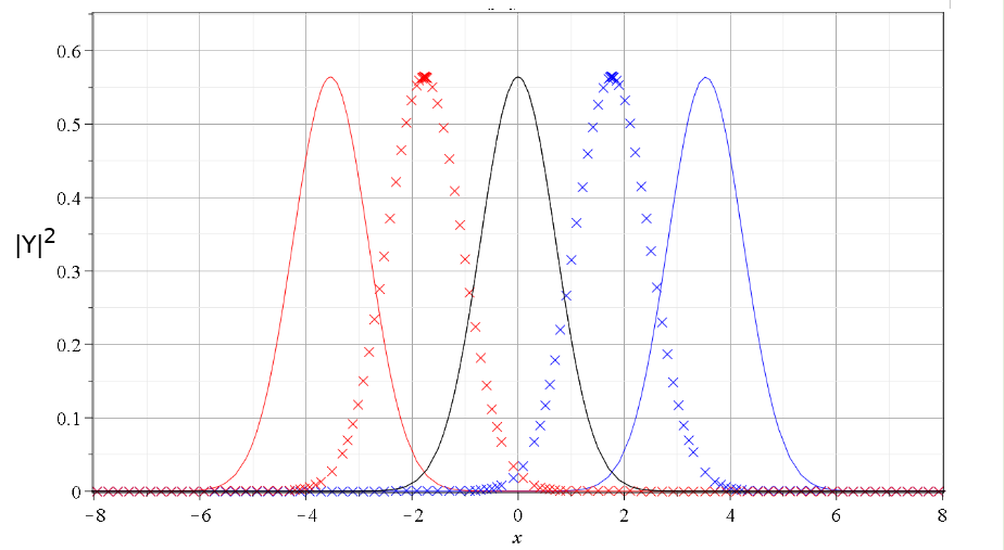
under the assumption that their overlap in phase space is sufficiently small. An example is given in Fig. 1, corresponding to $|A_{x}(0)|=|A_{y}(0)|=|A_{0}|=5/2$. This gives a negligible overlap, since $|\langle L|R\rangle|\,\sim\mathcal{O}(10^{-6})$.

Figure 1: The basis states of the qubit. At $t=0$ we have the solid blue curve on the right hand and the solid red curve on the left hand. They represent the absolute square of the wavefunctions of the coherent states $|R\rangle$ and $|L\rangle$ correspondingly. At $t=\pi/3$ the curves move towards $x=0$ (diagonal cross blue and red curves), while at $t=\pi$ they become identical at the center of the oscillation $x=0$. The oscillation period here is $T=2\pi$. (For both curves $|A_{0}|=5/2,\omega_{x}=1$, while $\sigma_{x}=0$ for the blue one and $\sigma_{x}=\pi$ for the red one.

2.3 Entanglement

The Von Neumann entropy ($VNE$) is the quantum mechanical extension of Gibbs entropy. For a state described by the density matrix $\rho$ (in a given basis) we have:

$$VNE=-tr[\rho\ln(\rho)]$$ (17)

which, for given eigenvectors ${|\Lambda_{i}\rangle}$ and eigenvalues ${\lambda_{i}}$ of $\rho$, reduces to

$$VNE=-\sum_{i}\lambda_{i}\ln(\lambda_{i}).$$ (18)

A non vanishing $VNE$ reflects the departure of a system from purity, since for a pure state we have $VNE=0$ ($\rho$ has one eigenvalue equal to 1). On the other hand $VNE$ takes a maximal value equal to $\ln(N)$ for $N$-dimensional Hilbert space in the case of a maximally mixed state. We note that the $VNE$ is preserved under unitary evolution since $VNE(\rho)=VNE(U\rho U^{\dagger})$, for any a unitary transformation $U$.

The $VNE$ can be used for the quantification of QE. In particular we can apply a partial trace operation over the degrees of freedom of one subsystem and then calculate the $VNE$ of the reduced density matrix which describes the remaining subsystem. The $VNE$ entropy of the reduced density matrix is called entanglement entropy ($EE$), and is a reliable measure of bipartite entanglement

$$EE\equiv VNE_{a}=VNE_{b}=-tr[\rho_{A}\ln(\rho_{A})]=-tr[\rho_{B}\ln(\rho_{B})].$$ (19)

The calculation of $VNE$ is in general a demanding task, since one needs to diagonalize the density matrix, whose dimension is in principle very large. This means that in general an analytical calculation of $EE$ is difficult (see for example[15]).

For a generic density matrix $\rho$ the linear entropy $LE$ is defined as

$$LE=1-\tr(\rho^{2}).$$ (20)

For a given $N\times N$ density matrix, the values of the $LE$ lie between $0$ and $1-1/N$ for a pure state and a maximally mixed state respectively. In fact $LE$ is an approximation of the $VNE$ and its calculation is simpler than that of $VNE$, since it does not require diagonalization of the density matrix. Consequently in the case of a pure state

$$\Psi(x,y)=\sqrt{R(x,y)}e^{iw(x,y)}$$ (21)

we can use as a measure of the bipartite entanglement the $LE$ of the reduced density matrix:

$$LE_{RED} =1-\tr(\rho_{A}^{2})=1-\tr(\rho_{B}^{2})$$ (22)

$$=1-\int dxdydx^{\prime}dy^{\prime}\Psi(x,x^{\prime})\Psi^{\dagger}(y,x^{\prime})\Psi(x,y^{\prime})\Psi^{\dagger}(y,y^{\prime}).$$

In order to study entanglement in Bohmian systems, Zander and Plastino showed in [16] that $LE_{RED}$ can be written as the sum of two quantities:

$$LE_{RED}=LE_{c}+LE_{p},$$ (23)

where

$$LE_{c}=1-\int dxdydx^{\prime}dy^{\prime}[R(x,x^{\prime})R(y,x^{\prime})R(x,y^{\prime})R(y,y^{\prime})]^{\frac{1}{2}}$$ (24)

is the ‘configuration entanglement’ and

$$LE_{p}=\int dxdydx^{\prime}dy^{\prime} \{1-\exp[i\Big{(}w(x,x^{\prime})-w(y,x^{\prime})-w(x,y^{\prime})-w(y,y^{\prime}\Big{)}]\}$$ (25)

$$\times[R(x,x^{\prime})R(y,x^{\prime})R(x,y^{\prime})R(y,y^{\prime})]^{\frac{1}{2}}$$

is the ‘phase entanglement’. The configuration entanglement expresses the lack of factorizability of the probability density $R(x,y)$, namely $R(x,y)\neq R_{1}(x)R_{2}(y)$, while the phase entanglement expresses the lack of additivity of the phase $w(x,y)$:

$$w(x,y)\neq w_{1}(x)+w_{2}(y).$$ (26)

In general, the analytical calculation of (24) and (25) is difficult and one needs to proceed numerically with algorithms like Cuhre or Monte-Carlo. However, in our case we study a system of two non-interacting subsystems. Consequently its entanglement remains constant over time. This means that a proper choice of the value of time $t$ (for a given wavefunction) can simplify the calculations. In our case if we assume that $c_{1},c_{2}$ are real, we can compute the entanglement at $t=0$, where the imaginary part of the wavefunctions $\Phi$ and $\Psi$ is equal to $0$ and consequently $LE_{RED}=LE_{c}$. In the case of $\Phi$ the multiple integral can be solved numerically. In the case of $\Psi$ we managed to find the solution analytically:

$$LE_{c}^{\Psi}=1-\Big{[}{c_{1}}^{4}-{c_{2}}^{4}+\left(-4{c_{1}}^{3}c_{2}+4{c_{1}}^{2}{c_{2}}^{2}-4c_{1}{c_{2}}^{3}\right){{\rm e}^{-4{\alpha_{0}}^{2}}}+2{c_{1}}^{2}{c_{2}}^{2}{{\rm e}^{-8{\alpha_{0}}^{2}}})\Big{]},$$ (27)

where $a_{0}\equiv|A_{0}|$. We note the fact that for all $\alpha_{0}$ $LE_{RED}=LE_{c}$ is independent from $\omega_{x},\omega_{y}$. In our case (large $\alpha_{0}$ and $c_{1},c_{2}\in[0,1]$) with $c_{1}^{2}+c_{2}^{2}=1$ we find

$$LE_{c}=1-\left({c_{1}}^{4}+{c_{2}}^{4})=2c_{2}^{2}(1-c_{2}^{2}\right)$$ (28)

Note that, for large $a_{0}$ our system becomes equivalent to a two-qubit spin system described by a $4\times 4$ density matrix in the standard basis $(\{|0\rangle,|1\rangle\})$, if we correspond $|0\rangle\to|R\rangle$ and $|1\rangle\to|L\rangle$. Then Eq. (28) is nothing else than the linear entropy of its reduced density matrix. However in this case it is trivial to calculate the $VNE$ of the reduced density matrix for both states (10) and (11), the so called entanglement entropy $EE$:

$$EE=-\Big{(}|c_{1}|^{2}\ln(|c_{1}|^{2})+|c_{2}|^{2}\ln(|c_{2}|^{2}))=(1-|c_{2}|^{2})\ln(1-|c_{2}|^{2})+|c_{2}|^{2}\ln(|c_{2}|^{2}))$$ (29)

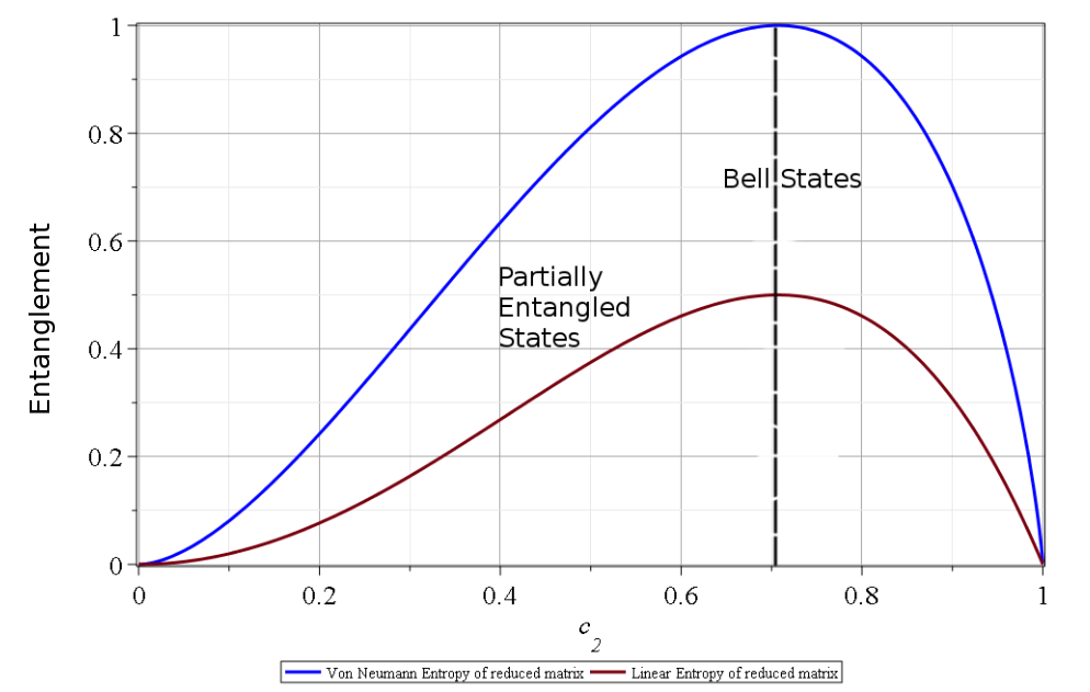
Figure 2 shows the $LE_{RED}$ (Eq. (28)) and $EE$ (Eq. (29)) for different values of the coefficient $c_{2}$. Both of them exhibit the same behaviour for all values of $c_{2}$, hence $LE_{RED}$ is a reliable measure for the quantification of entanglement. In particular, the maximum entanglement takes place when $c_{2}=\sqrt{2}/2$ (Bell states).

Figure 2: The entanglement as a function of $c_{2}$, measured by the $EE$ of Eq. (29) (blue curve) and $LE_{RED}$ of Eq. (28) (bordeuax curve). It is common for both states $\Psi$ and $\Phi$. We observe that $EE=0$ for $c_{2}=0$ and $c_{2}=1$ , something expected since in that cases we have product states. The maximum value of $LE_{RED}^{max}=1/2$ corresponds to $c_{2}=\frac{\sqrt{2}}{2}$, namely in the case of a Bell state (maximally entangled state). In that case the $EE_{max}$ is equal to $\ln(2)$, or equal to 1 if we use 2 as the basis of the logarithm (as we have done here), which is the case in quantum information theory. All of the other values of $c_{2}$ refer to partially entangled states.

3 Bohmian equations and nodal points

The Bohmian trajectories guided by a wavefunction $\Psi=\Psi_{R}+i\Psi_{I}$ are found via the Bohmian equations

$$m_{i}\frac{dx_{i}}{dt}=\frac{\hbar}{G}\Big{(}\frac{\partial\Psi_{I}}{\partial x_{i}}\Psi_{R}-\frac{\partial\Psi_{R}}{\partial x_{i}}\Psi_{I}\Big{)},\quad i=1,2,\dots$$ (30)

with $G=\Psi_{R}^{2}+\Psi_{I}^{2}$. Hereafter we work with $\hbar=m_{1}=m_{2}=1$. The Bohmian equations for the state $\Psi$ are:

$$\frac{dx}{dt}=-\frac{\sqrt{2\omega_{x}}a_{0}\left[A\cos\left(\omega_{x}t\right)+B\sin\left(\omega_{x}t\right)\right]}{G}$$ (31)

$$\frac{dy}{dt}=\frac{\sqrt{2\omega_{y}}a_{0}\left[A\cos\left(\omega_{y}t\right)+B\sin\left(\omega_{y}t\right)\right]}{G}$$ (32)

and for the state $\Phi$ are:

$$\frac{dx}{dt}=-\frac{\sqrt{2\omega_{x}}a_{0}\left[C\cos\left(\omega_{x}t\right)+D\sin\left(\omega_{x}t\right)\right]}{G^{\prime}}$$ (33)

$$\frac{dy}{dt}=-\frac{\sqrt{2\omega_{y}}a_{0}\left[C\cos\left(\omega_{y}t\right)+D\sin\left(\omega_{y}t\right)\right]}{G^{\prime}}$$ (34)

where

$$A=2c_{1}c_{2}{{\rm e}^{2f_{x}+2f_{y}}}\sin\left(2(g_{x}-g_{y})\right)$$ (35)

$$B=c_{1}^{2}e^{4f_{x}}-c_{2}^{2}e^{4f_{y}}$$ (36)

$$G=2c_{1}c_{2}{{\rm e}^{2f_{x}+2f_{y}}}\cos\left(2(g_{x}-g_{y})\right)+{{\rm e}^{4f_{y}}}{c_{2}}^{2}+{{\rm e}^{4f_{x}}}{c_{1}}^{2}$$ (37)

$$C=2c_{1}c_{2}{{\rm e}^{2f_{x}+2f_{y}}}\sin\left(2(g_{x}+g_{y})\right)$$ (38)

$$D={c_{1}}^{2}{{\rm e}^{4f_{x}+4f_{y}}}-{c_{2}}^{2}$$ (39)

$$G^{\prime}={c_{1}}^{2}{{\rm e}^{4f_{x}+4f_{y}}}+2c_{1}c_{2}{{\rm e}^{2f_{x}+2f_{y}}}\cos\left(2(g_{x}+g_{y})\right)+{c_{2}}^{2}$$ (40)

with

$$f_{x}=\sqrt{2\omega_{x}}a_{0}\cos\left(\omega_{x}\,t\right)x,\quad f_{y}=\sqrt{2\omega_{y}}a_{0}\cos\left(\omega_{y}\,t\right)y,$$ (41)

$$g_{x}=\sqrt{2\omega_{x}}a_{0}\,\sin\left(\omega_{x}\,t\right)x,\quad g_{y}=\sqrt{2\omega_{y}}a_{0}\,\sin\left(\omega_{y}\,t\right)y$$ (42)

A useful quantity for the identification of chaos is the “finite time Lyapunov characteristic number” LCN. If $\xi_{k}$ is the length of the deviation vector between two nearby trajectories at the time $t=\kappa t_{0},\,\kappa=1,2,\dots$, then the quantity

$$\alpha_{\kappa}=\ln\Big{(}\frac{\xi_{\kappa+1}}{\xi_{\kappa}}\Big{)}$$ (43)

is the so called “stretching number” and the “finite time Lyapunov characteristic number” is given by the equation:

$$\chi=\frac{1}{\kappa t_{0}}\sum_{i=1}^{\kappa}\alpha_{i}$$ (44)

The LCN is the limit of $\chi$ when $\kappa\to\infty$ and the ratio $\frac{\xi_{\kappa+1}}{\xi_{\kappa}}$ is computed by the variational equations of motion (see [17, 18]). LCN is positive for chaotic trajectories and equal to zero for ordered trajectories.

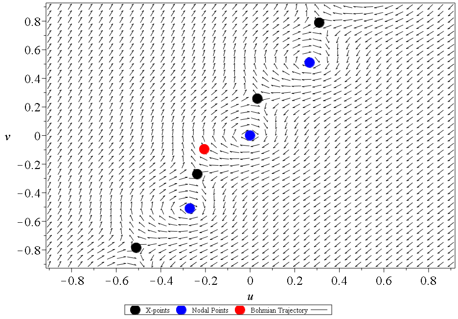
In previous works we made a detailed investigation of order and chaos in BQM [19, 20, 21, 22]. In the close neighbourhood of nodal points, which are defined as solutions of the system:

$$\Re\Psi=\Im\Psi=0,$$ (45)

the Bohmian particles evolve very fast and form spirals around them. In a frame comoving with a nodal point, the nodal point is accompanied by a second stationary point of the flow, the X-point. At the X-point the Bohmian velocity becomes equal to that of the moving node

$$\frac{dx}{dt}=V_{xnod},\quad\frac{dy}{dt}=V_{ynod}.$$ (46)

Together they form the nodal point-X-point complex (NPXPC), a characteristic geometrical structure of the Bohmian flow in the vicinity of a certain moving nodal point. We have shown that the NPXPC are responsible for the emergence of chaos in two and three dimensional Bohmian systems (see also [23, 24]). Whenever a trajectory approaches a NPXPC it gets scattered by the X-point and the stretching number undergoes a positive shift. The cumulative action of NPXPCs on the trajectories produces chaos: two arbitrarily close initial conditions produce trajectories whose distance grows exponentially in time. On the other hand, the trajectories that do not interact with the NPXPCs are ordered.

In our case the nodal points of the $\Psi$ (Eq. 10) read:

$$x_{nod}={\frac{\sqrt{2}\left(k\pi\,\cos\left(\omega_{y}\,t\right)+\sin\left(\omega_{y}\,t\right)\ln\left(\left|{\frac{c_{1}}{c_{2}}}\right|\right)\right)}{4\sqrt{\omega_{x}}a_{0}\,\sin\left(\omega_{xy}t\right)}}$$ (47)

$$y_{nod}={\frac{\sqrt{2}\left(k\pi\,\cos\left(\omega_{x}t\right)+\sin\left(\omega_{x}t\right)\ln\left(\left|{\frac{c_{1}}{c_{2}}}\right|\right)\right)}{4\sqrt{\omega_{y}}a_{0}\,\sin\left(\omega_{xy}\,t\right)}}$$ (48)

with $k\in Z$, $k$ even for $c_{1}c_{2}<0$ or odd for $c_{1}c_{2}>0$ and $\omega_{xy}\equiv\omega_{x}-\omega_{y}$. Consequently there exist infinitely many nodal points in space. Similarly the nodal points in the case of $\Phi$ (Eq. 11) read:

$$x_{nod}={\frac{\sin\left(\omega_{x}t\right)\sqrt{2}\left(k\pi\,\cos\left(\omega_{y}\,t\right)+\ln\left(\Big{|}{\frac{c_{1}}{c_{2}}}\Big{|}\right)\sin\left(\omega_{y}\,t\right)\right)}{2\sqrt{\omega_{x}}a_{0}\left(\cos\left(\omega_{y}t\right)-\cos\left(t\left(2\,\omega_{x}-\omega_{y}\right)\right)\right)}}$$ (49)

$$y_{nod}=-{\frac{\sqrt{2}\left(k\pi\cos\left(\omega_{x}\,t\right)+\sin\left(\omega_{x}\,t\right)\ln\left(\left|{\frac{c_{1}}{c_{2}}}\right|\right)\right)}{4\sqrt{\omega_{y}}a_{0}\sin\left(\omega_{xy}t\right)}}$$ (50)

where again $k$ is even for $c_{1}c_{2}<0$ or odd for $c_{1}c_{2}>0$. Equations (47, 48, 49) and (50) show that in general there exist nodal points evolving in space-time for different $\omega_{x},\omega_{y}$ and various amounts of entanglement (different $c_{2}$). The state $\Psi$ gives:

$$\frac{y_{nod}}{x_{nod}}=\frac{k\pi\,\cos\left(\omega_{x}t\right)+\sin\left(\omega_{x}t\right)\ln\left(\left|{\frac{c_{1}}{c_{2}}}\right|\right)}{k\pi\,\cos\left(\omega_{y}\,t\right)+\sin\left(\omega_{y}\,t\right)\ln\left(\left|{\frac{c_{1}}{c_{2}}}\right|\right)}$$ (51)

while the state $\Phi$ gives

$$\frac{y_{nod}}{x_{nod}}=\frac{-\sqrt{\omega_{x}}\left(\cos\left(\omega_{x}t\right)k\pi+\sin\left(\omega_{x}t\right)\ln\left(\left|{\frac{c_{1}}{c_{2}}}\right|\right)\right)\Big{(}\cos\left(\omega_{y}t\right)-\cos\left((2\omega_{x}\!-\!\omega_{y})t\right)\Big{)}}{2\sqrt{\omega_{y}}\sin\left(\omega_{xy}t\right)\sin(\omega_{x}t)\Big{[}k\pi\cos\left(\omega_{y}t\right)+\sin\left(\omega_{y}t\right)\!+\!\ln\left(\left|{\frac{c_{1}}{c_{2}}}\right|\right)\Big{]}}$$ (52)

Finally we note that with the tranfsormation $(t\to-t,k^{\prime}\to-k)$ one finds the same values of $x_{nod},y_{nod}$ in both cases. Thus, the same nodal points appear in the plane $(x,y)$ at the times $t$ and $-t$.

4 Trajectories

4.1 Incommensurable frequencies

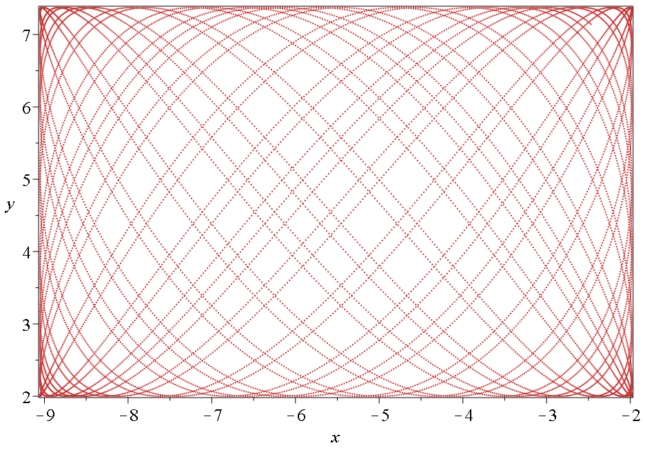
When the oscillators have incommensurable frequencies, in the extreme case of a product state the trajectories are of Lissajous type. For example Fig. 3 shows a trajectory in the state $Y_{R}(x,t)Y_{L}(y,t)$ ($c_{2}=0$). In this case the Bohmian equations are decoupled, the nodal points are at infinity and the motion is ordered.

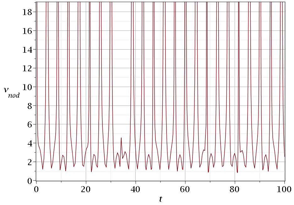
This behaviour changes with the onset of entanglement, namely with the increase of $c_{2}$. In Fig. 4 we show the trajectories of two different nodal points with $k=1$ and $k=3$ for the wavefunction $\Psi$. The frequencies are $\omega_{x}=1$ and $\omega_{y}=\sqrt{3}$. The coefficient $c_{2}$ is set equal to $2\times 10^{-5}$, namely the entanglement is extremely small, $EE\simeq 8\times 10^{-10}$. Even with this slight perturbation we observe that the trajectories of the nodal points enter repeatedly the region of space where the support of the wavefunction is strong and then go repeatedly to infinity with very high velocities (Fig. 5). Whenever a Bohmian particle comes close to one of the infinitely many NPXPCs, there is a sudden spike in the evolution of the stretching number. Consequently, chaos emerges as shown in Fig. 6.

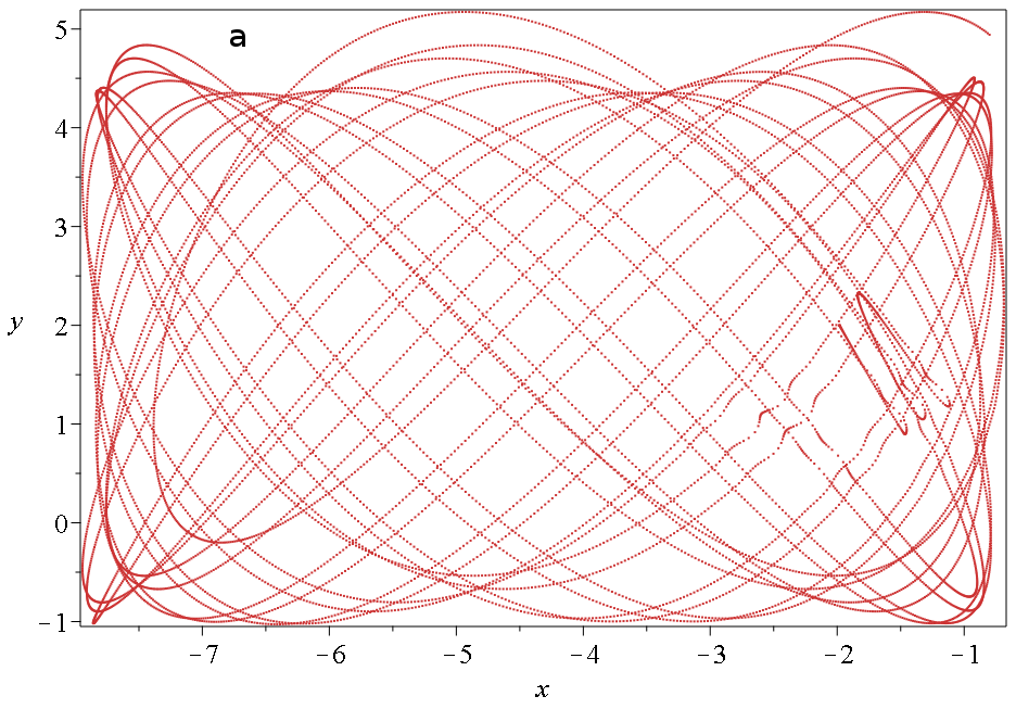
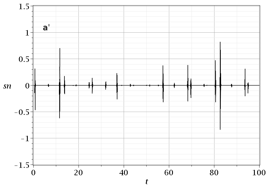
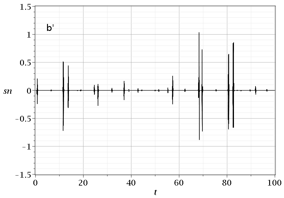
Figure 6a,a’ shows what happens in the case of the state $\Psi$ when $c_{2}=2\times 10^{-6}$: the initial Lissajous curve becomes deformed and its size changes. However the trajectory still evolves in a almost confined region of physical space up for $t\in[0,100]$ and the action of the NPXPCs is limited to the deformation of the initial Lissajous curve as we can see in the scattering events for $-2\leq x\leq-1$ and $1\leq y\leq 2$, which correspond to the initial shifts of the stretching number.

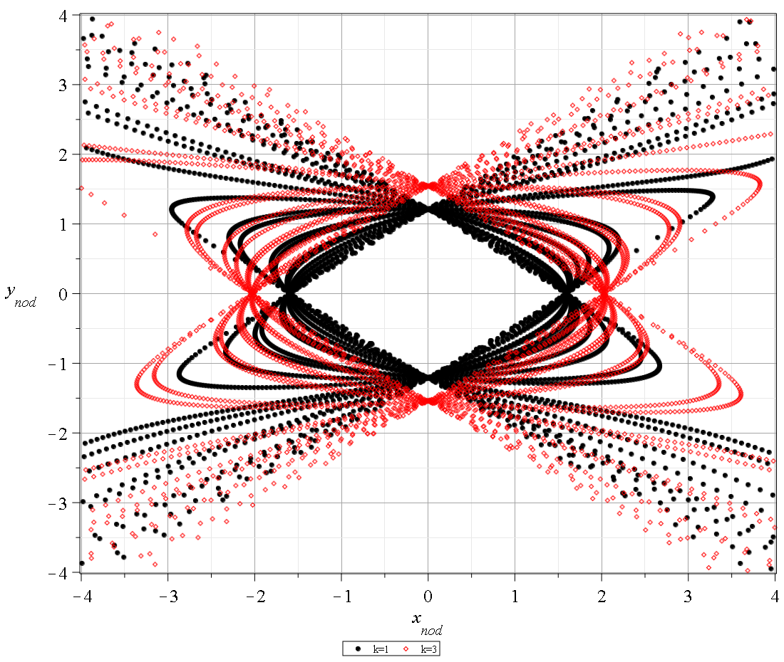
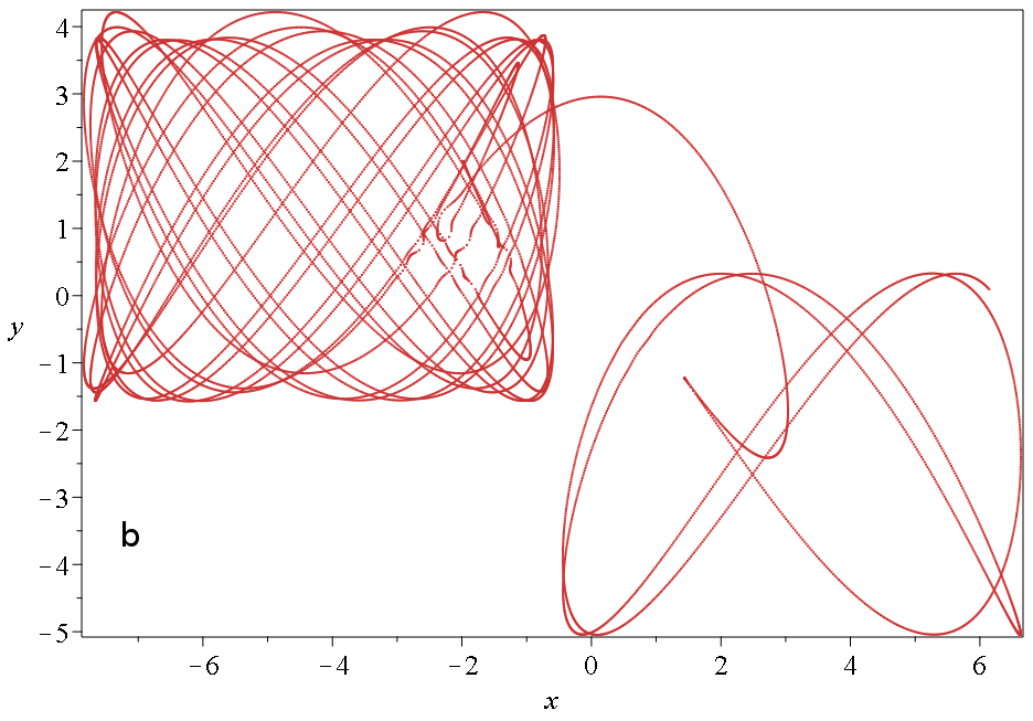
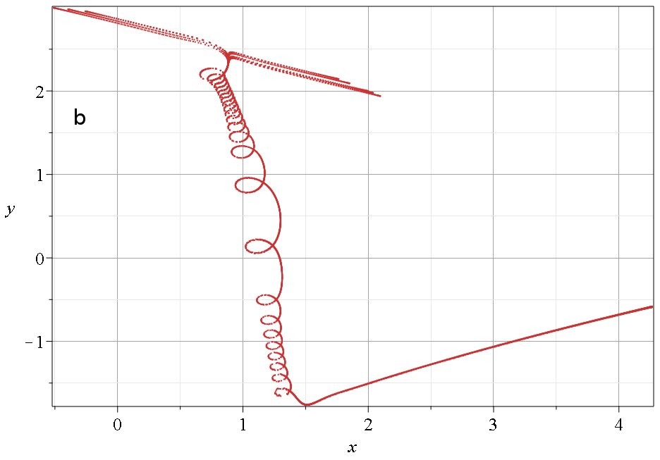
However for $c_{2}=2\times 10^{-5}$ (Fig. 6b,b’) besides the deformation of the initial Lissajous type curve, there is a strong scattering event which forces the trajectory to exit the initial region and move to an other region on the lower right part of the figure with almost the same horizontal and vertical dimensions. We call ‘derailment time’ the time when such a major scattering event takes place. In Fig. 6 the derailment time is $t_{d}\simeq 82.66$. Indeed the stretching number undergoes a strong positive shift at $t_{d}$. This is shown in detail in Fig. 7. Multiple NPXPCs cross the plane $(x,y)$ at $t_{d}$. The nodal points are colored blue, the X-points are black. The Bohmian trajectory is close to one of the X-points of the multiple NPXPCs, hence subject to scattering.

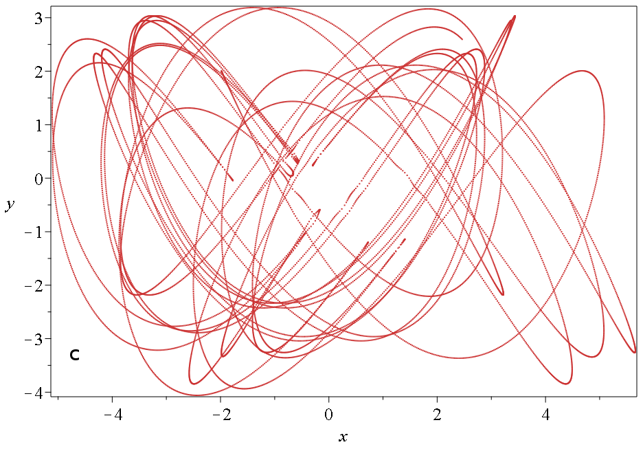
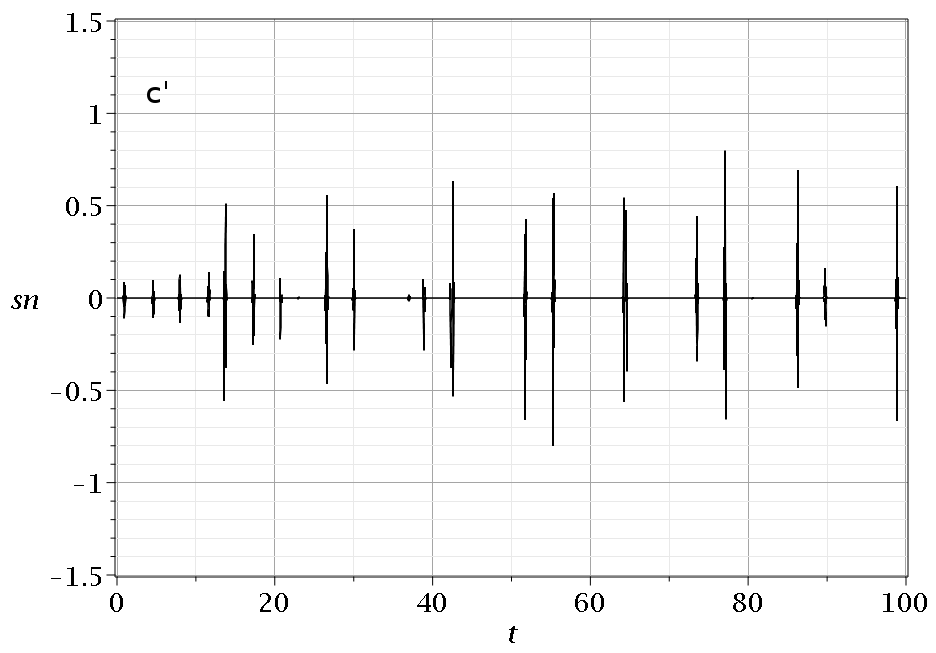
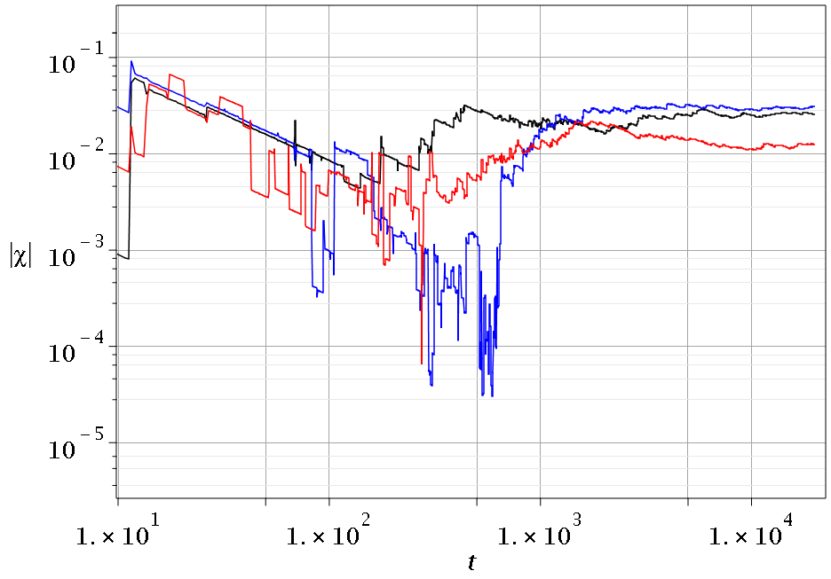
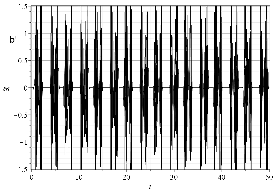
Increasing $c_{2}$ in the extreme case of a maximally entangled state $(c_{1}=c_{2}=\sqrt{2}/2)$ we observe chaos immediately through a large number of scattering events, as shown in Fig. 6c,c’ and the corresponding time series of the stretching number [18]). The finite time Lyapunov characteristic number $\chi$ for all cases is given in Fig. 8.

Figure 3: A Bohmian trajectory in the case of the product state $Y_{RL}=Y_{R}Y_{L}$ for $t\in[0,100]$. It is a typical Lissajous curve. $(x(0)=-2,y(0)=2,\omega_{x}=1,\omega_{y}=\sqrt{3})$

Figure 4: The nodal trajectories of the state $\Psi$ for $k=1$ (black dots) and $k=3$ (red squares) for $t\in[0,100]$. ($\omega_{x}=1,\omega_{y}=\sqrt{3},c_{2}=2\times 10^{-5}$). Entanglement brings the nodal points (and consequently the X-points) into the region where the wavefunction has strong support and produces chaos.

Figure 5: The absolute value of the velocity of a certain nodal point of the state $\Psi$ with $k=1,\omega_{x}=1,\omega_{y}=\sqrt{3}$. We observe the repeated fast motion to infinity.

Figure 6: Bohmian trajectories and the corresponding variations of the stretching numbers for the state $\Psi$. Entanglement brings chaos and changes significantly the behaviour of the Bohmian trajectory from that of a Lissajous curve. a) If we set $c_{2}=2\times 10^{-6}$ we see that the initial Lissajous curve becomes deformed and its dimensions change. When the orbit approaches an X-point we have an abrupt change of the stretching number. b) For $c_{2}=2\times 10^{-5}$ the behaviour changes drastically. At time $t=82.66$ there is a strong scattering event (b’) which derails the trajectory outside the initial region. c) If we increase entanglement chaos becomes apparent immediately as in the case of a maximally entangled state with $c_{2}=\sqrt{2}/2$. $(x(0)=-2,y(0)=2,\omega_{x}=1,\omega_{y}=\sqrt{3})$, which is followed by many abrupt changes of the stretching number (c’).

Figure 7: The NPXPCs of the state $\Psi$ at $t=t_{d}\simeq 82.66$. We observe that the Bohmian particle (red point) is close to one of the X-points. The interaction of this particle with the X-point produces a jump in the stretching number. Such close encounters between particles and X-points lead to a positive LCN, and consequently to chaos $(x(0)=-2,y(0)=2,\omega_{x}=1,\omega_{y}=\sqrt{3},c_{2}=2\times 10^{-5})$

Figure 8: The absolute value of the finite time Lyapunov characteristic number $\chi$ for the three cases of Fig. 6 (state $\Psi$) in logarithmic axes. The blue curve corresponds to $c_{2}=2\times 10^{-6}$, the black curve corresponds to $c_{2}=2\times 10^{-5}$ and the red curve corresponds to $c_{2}=\sqrt{2}/{2}$. The sudden droppings of $|\chi(t)|$ to very small values (on a logarithmic scale) correspond to the crossings of the axis $\chi(t)=0$ during the oscillatory motion of $\chi(t)$ between positive and negative values. However, we observe that for times larger than $t=1.5\times 10^{4}$ $\chi(t)$ stabilizes at a positive value. Consequently the trajectories are chaotic.

4.2 Commensurable frequencies and the special case of isotropic oscillators

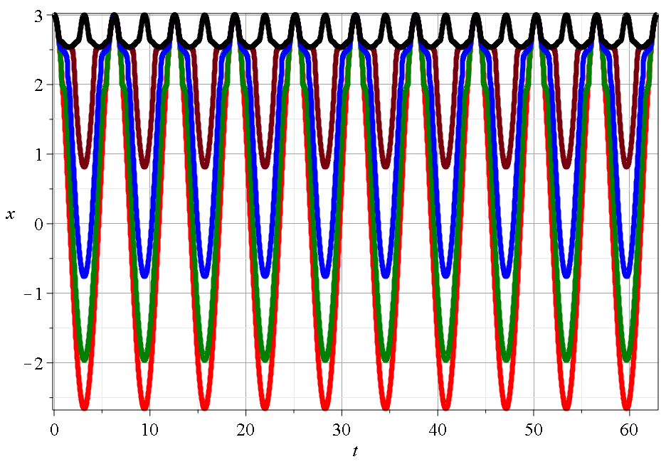
In Fig.1 we show the oscillatory behavior of the absolute value of two one-dimensional coherent states with the same frequency $\omega_{x}=\omega_{y}=1$ and amplitude $|A_{0}|=5/2$ which at $t=0$ start from the right and the left limiting points of the oscillation (blue and red curve respectively). This is done by choosing $\sigma=0$ for the first one and $\sigma=\pi$ for the second one. We observe that at $t=\pi/3$ the two curves have a complete spatial overlap at $x=0$ (black curve), which is totally different from their almost vanishing overlap in phase space.

In Fig. 9 we present a case where $\omega_{x}=2,\omega_{y}=1$ for a certain initial condition $x(0)=y(0)=2$ and for different values of $c_{2}$ in the state $\Psi$. We note that in the absence of entanglement, namely in the case of a product state, the trajectory is periodic, since it is the composition of two oscillations with $\omega_{x}/\omega_{y}$ is a rational number. The insertion of entanglement implies the existence of nodes. However, with some algebra one can see that Eqs. (31) and (32) yield periodic solutions. In fact if $\omega_{1}/\omega_{2}$ is an irreducible ratio $s_{1}/s_{2}$, where $s_{1},s_{2}$ are positive integers, then the period of the system is $T=2\pi s_{2}/\omega_{y}$. Moreover there is time reversal antisymmetry, namely for $t^{\prime}=-t$ we get $dx/dt^{\prime}=-dx/dt$ and $dy/dt^{\prime}=-dy/dt$. Finally for $t=0$ we have $dx/dt=dy/dt=0$. Consequently the motion is periodic with reflection at $t=0$. The same property holds for the state $\Phi$.

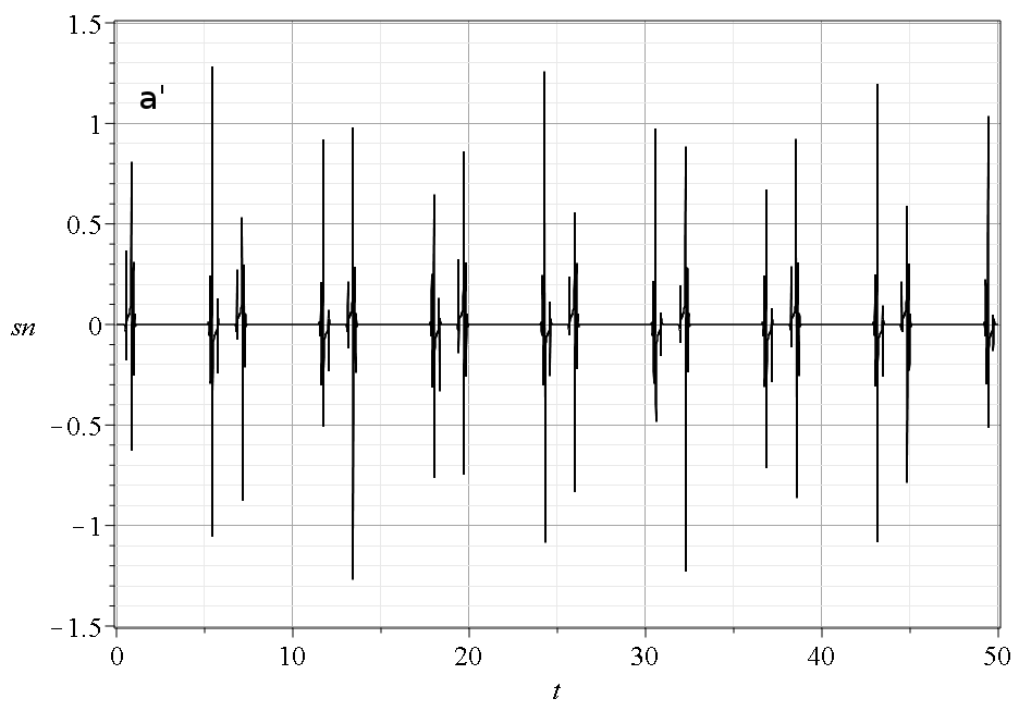
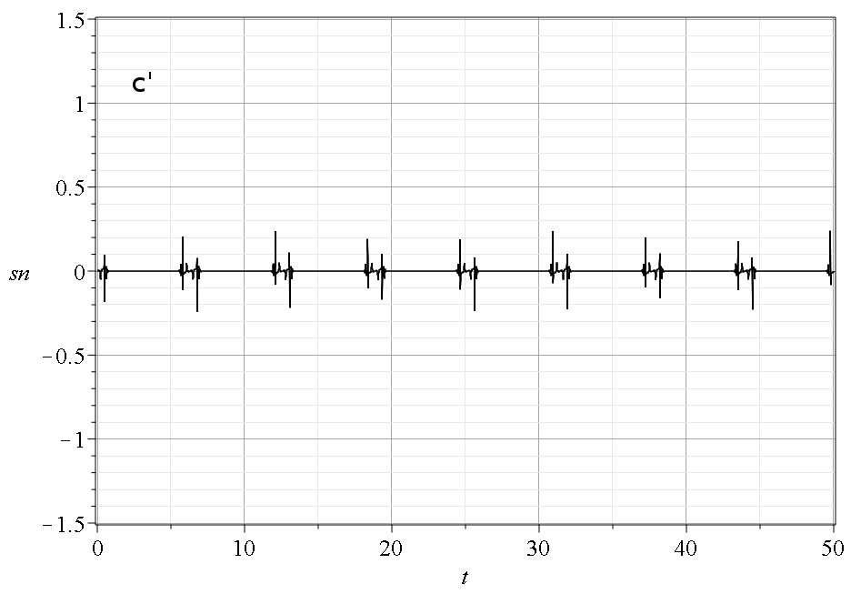
In Fig. 9a,a’, while the amount of entanglement is extremely small, one observes strong scattering events in the stretching numbers. For a larger, but still small, value of entanglement, we observe spiral motion (Fig. 9b,b’). This is the typical behaviour of a Bohmian trajectory close to a moving nodal point. In this case scattering effects are very strong. Finally for a maximally entangled state the scattering effects are milder (Fig. 9c,c’).

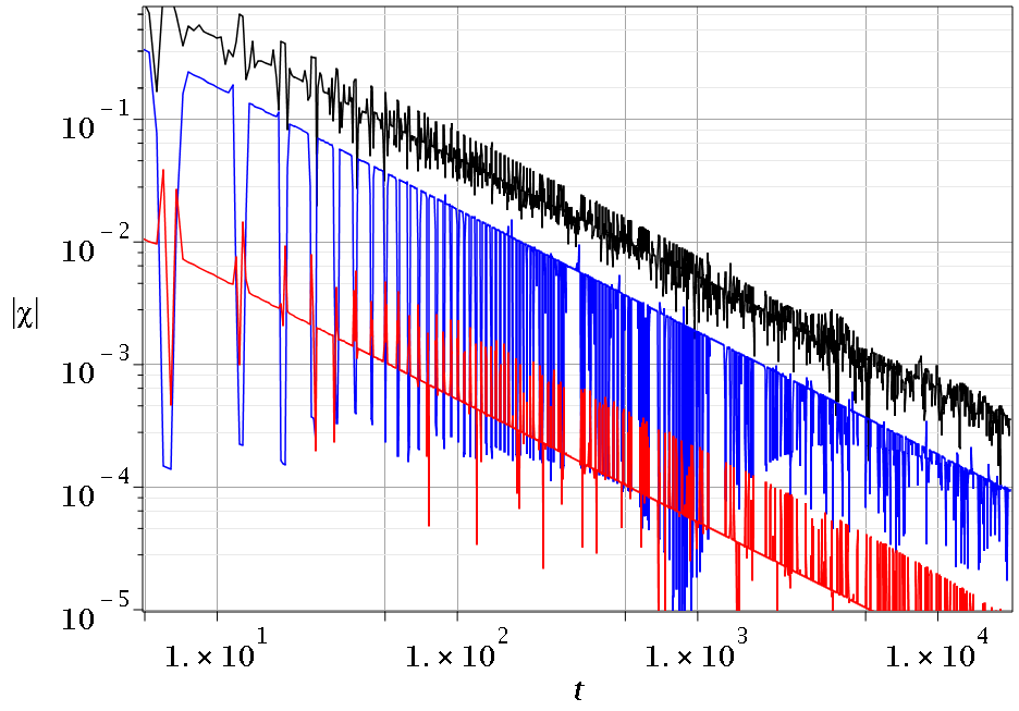
In all cases $\chi$ vanishes in the course of time. In Fig. 10, the blue curve corresponds to $c_{2}=2\times 10^{-6}$, the black curve corresponds to $c_{2}=2\times 10^{-5}$ and the red curve corresponds to $c_{2}=\sqrt{2}/{2}$. However, the system may appear as ‘effectively chaotic’ ($\chi$ large) for transient times long enough but shorter than the period. Conversely, a system with incommensurable ratio $\omega_{x}/\omega_{y}$ may appear as ‘effectively ordered’ ($\chi$ going temporarily to zero) at times corresponding to approximate periods defined by rational approximation of the ratio $\omega_{x}/\omega_{y}$. For the details about the distinction between effectively chaotic and effectively ordered orbits see [25].

Figure 9: Three Bohmian trajectories of the state $\Psi$ with common initial condition $x(0)=y(0)=2$ for $\omega_{x}=2,\omega_{y}=1$. a) $c_{2}=2\times 10^{-6}$, b) $c_{2}=2\times 10^{-5}$ and c) $c_{1}=c_{2}=\sqrt{2}/2$. The evolution of the corresponding stretching numbers is shown in (a’), (b’) and (c’) respectively. The spikes in the latter plots correspond to scattering events of the trajectories by the NPXPCs. These trajectories are all periodic, but they exhibit considerable complexity due to the interaction with the NPXPCs.

Figure 10: The absolute value of the finite time Lyapunov characteristic number $\chi$ for the three cases of Fig. 9 (state $\Psi$) in logarithmic axes. The blue curve corresponds to $c_{2}=2\times 10^{-6}$, the black curve corresponds to $c_{2}=2\times 10^{-5}$ and the red curve corresponds to $c_{2}=\sqrt{2}/{2}$. We observe the decrease of $\chi$ over the course of time according to a power law, which is a signature of ordered trajectories. Although there exist NPXPCs there is no chaos production, since the motion is periodic.

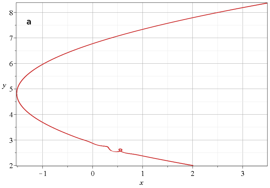
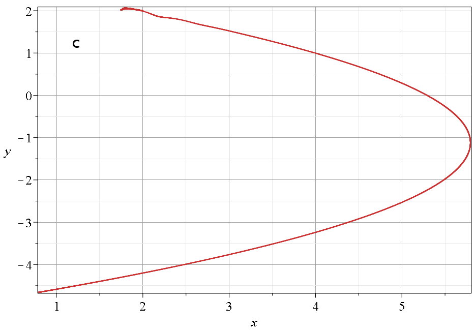
In the extreme case where $\omega_{x}=\omega_{y}$, namely when the oscillators are isotropic, we get for the state $y_{nod}/x_{nod}=1$ for the state $\Psi$. From the common denominator of Eqs. (47) and (48), both $x$ and $y$ go to infinity when $\omega_{xy}=0$. Consequently as $\omega_{xy}\to 0$ the nodal points disappear very fast along the line $y=x$ and we find ordered trajectories. Similarly for the state $\Phi$ we have $(x,y)\to\infty$ as $\omega_{x}\to\omega_{y}$ with $y_{nod}/x_{nod}=-1$ and again we find ordered trajectories.

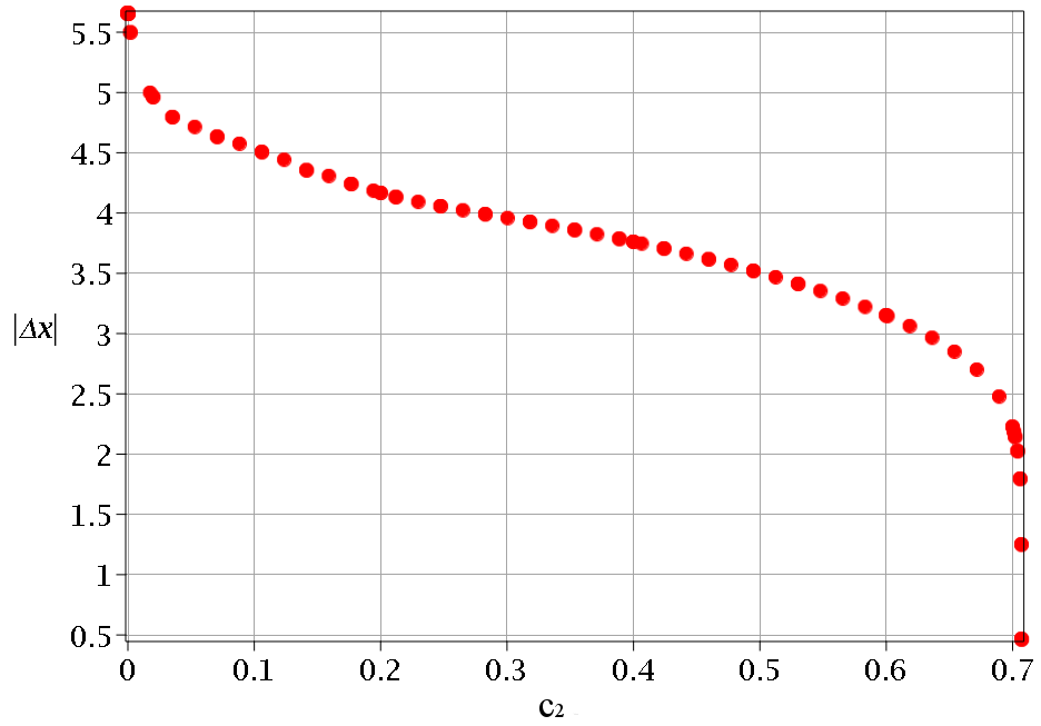
In fact one can easily check that in the case of the isotropic oscillators both states produce ordered trajectories characterized by integrals of motion: the state $\Phi$ gives $y-y(0)=x-x(0)$ while $\Psi$ gives $y-y(0)=-(x-x(0))$. Consequently the particles move on certain straight lines parallel to the diagonals $x=\pm y$ defined from their initial positions. Here the effect of the increase of the entanglement is a gradual deformation and spatial confinement of the oscillatory motion which occurs when the system is separable ($c_{2}=0$). In Fig. 11 we observe this deformation for the same initial value $x(0)=3,y(0)=2$ and different values of $c_{2}$ in the state $\Psi$. For small values of $c_{2}$ (small entanglement) the trajectory is similar to that of the separable case, with only a mild deformation at $x\simeq 2$. The range of motion in the x-axis gets smaller with the increase of $c_{2}$, while the range of motion in the y-axis is affected via the integral of motion $y=y(0)-(x-x(0))$ and becomes smaller with the increase of entanglement as well. Moreover we observe that in the partially entangled states the leading Fourier component is $\sin(t)$, while higher harmonics ($\sin(mt),\,m=2,3,\dots)$ become increasingly important as the entanglement increases. In fact, the leading Fourier term in the maximally entangled state is $\sin(2t)$.

We note here that the integration of these seemingly simple ordered trajectories becomes difficult when we approach the maximally entangled state where $c_{1}=c_{2}=\sqrt{2}/2$, due to the high degree of nonlinearity. For $c_{2}\in[0.7,\sqrt{2}/2\simeq 0.707106781]$ one needs very accurate numerical integration since even with a small time step, for example a 4th order Runge-Kutta scheme with time step of order $\mathcal{O}(10^{-4})$, there is a large accumulative error over the course of time, which leads to erroneous non-periodic solutions with respect to the initial conditions, namely to trajectories that do not reach the initial conditions in every cycle. In the case of adaptive numerical schemes, like 4th order Runge-Kutta-Fehlberg with 5 order error estimator, one needs very small tolerance in absolute and relative errors, even for short time monitoring of the solution. In order to monitor the trajectory correctly in the relatively wide time window of the first 10 cycles of motion ($0\to 20\pi$), we applied the Dormand Prince method of 8th order with 5th order error estimator, and with absolute error tolerance $atol=10^{-18}$ and relative error tolerance $rtol=10^{-17}$ ([26]). This peculiar behaviour of the system in the close region of maximally entangled state stems from the high contribution of all nonlinear terms of the equations of motion, which in the case of maximally entangled state becomes of the same order of magnitude. In Fig. 12 we present the variation of $|\Delta x|$ for different values of the coefficient $c_{2}$. In the cases of small and large entanglement we observe a fast decrease of $|\Delta x|$, while for intermediate values of $c_{2}$ the decrease is almost linear.

To sum up, we see that in the presence of integrability the QE affects the trajectories differently than in the case of non-integrability. It does not change significantly the shape of the joint evolution, but it dictates the range of motion in both axes.

Figure 11: The motion of the Bohmian particle in the case $\omega_{x}=\omega_{y}=1$ for a given initial condition and different amounts of entanglement (state $\Psi$). Red curve: $c_{2}=2\times 10^{-5}$, green curve: $c_{2}=2\times 10^{-2}$, blue curve: $c_{2}=4\times 10^{-1}$ burgundy curve: $c_{2}=0.701$ and black curve: $c_{2}=\sqrt{2}/2\simeq 0.707$. The larger the entanglement, the smaller the range of motion. The period of all orbits is $2\pi$ except from the maximal entanglement case (black curve), where is equal to $\pi$. In this case, the entanglement introduces no chaos but affects the Fourier spectrum of the periodic trajectories.

Figure 12: The range of motion $|\Delta x|$ in the x-axis as a function of the coefficient $c_{2}$ (and consequently of entanglement) in the case of Fig. 11. We observe the fast decrease of $|\Delta x|$ in the regions of small and large values of $c_{2}$. For intermediate values of $c_{2}$ the range of motion exhibits an approximatively linear decrease. Entanglement differentiates clearly the trajectories in the extreme cases of $c_{2}=0$ (product state) where $|\Delta x|=5.657$ and for $c_{2}=\sqrt{2}/2$ (maximally entangled state) where $\Delta x$ is minimum and equal to $0.464$.

5 Conclusions

In the present work we studied the effect of quantum entanglement (QE) on the Bohmian trajectories of a simple bipartite system, composed of two entangled one dimensional canonical coherent states. Our main results are:

1. The presence of entanglement plays a crucial role for the evolution of Bohmian particles. In fact a very small amount of entanglement which can be thought of as a small perturbation in a product state, suffices to bring strong chaos by activating the nodal point-X-point mechanism.

2. A simple (but highly non-linear) two-qubit Bohmian system has infinitely many nodal point-X-point complexes (NPXPCs) which not only cover large parts of physical space, but also evolve very fast in time and scatter most of the Bohmian trajectories. Consequently for every non-vanishing value of entanglement the system is characterized by complex dynamics.

3. They key parameter of the system is the frequency ratio $\omega_{1}/\omega_{2}$. In the case of anisotropic oscillators with incommensurable frequencies entanglement is a prerequisite for the existence of NPXPCs which scatter the trajectories and produce chaos.

4. In the case of anisotropic oscillators with commensurable frequencies we found that the trajectories are complicated but periodic. Consequently we have ‘effectively chaotic’ trajectories for transient times smaller than the period $T$ of the system, but the motion turns eventually to be ordered.

5. When the oscillators are isotropic the NPXPCs dissapear (go to infinity) and the system is integrable. The trajectories are confined to certain straight lines depending on the initial conditions. In that case the presence of entanglement can not affect the integrability of the system, but it changes the shape of the trajectories. We monitored the range of motion as a function of the coefficient $c_{2}$ and found that the larger the $c_{2}$, the smaller the $|\Delta x|$. For small and large values of $c_{2}$ the variation of $|\Delta x|$ was fast, while for intermediate values it was almost linear with respect to $c_{2}$. Furthermore, the increase of the entanglement implies a change in the Fourier components of the periodic motion. In the extreme case of a maximal entangled state the leading Fourier term changes from $\sin(t)$ to $\sin(2t)$.

In this paper we connected the evolution of Bohmian trajectories with the degree of the entanglement of their guiding wavefunction. We worked with the simplest non-trivial case, namely two entangled qubits. According to our remarks (iii) and (iv) above, the entanglement leads in most cases to chaos, in agreement with the results of [11]. However, there are also cases in which the entanglement does not produce chaos, but it can still affect the spectrum of the regular trajectories. An interesting question for further study is the relation between the chaotic/regular Bohmian trajectories and the (possibly) conserved mean values of several quantities such as energy, linear momentum, angular momentum etc.[27] in entangled bipartite systems.

The simple wavefunctions of the present paper provide useful information about the phenomenology of the entanglement in Bohmian trajectories. This is a necessary step towards the exploitation of Bohmian trajectories for a trajectory-based characterization of QE (construction of indicators and measures), with possible applicability in the case of high-dimensional bipartite systems, or multipartite systems, where the quantification of entanglement remains an open problem.

References

- [1] Bohm D 1952 Phys. Rev. 85(2) 166
- [2] Bohm D 1952 Phys. Rev. 85(2) 180
- [3] Horodecki R, Horodecki P, Horodecki M and Horodecki K 2009 Rev. Mod. Phys. 81 865
- [4] Mintert F, Carvalho A R, Kuś M and Buchleitner A 2005 Phys. Rep. 415 207–259
- [5] Nielsen M A and Chuang I L 2004 Quantum Computation and Quantum Information (Cambridge Series on Information and the Naturciences) (Cambridge University Press)
- [6] Durt T and Pierseaux Y 2002 Phys. Rev. A 66 052109
- [7] Braverman B and Simon C 2013 Phys. Rev. Lett. 110 060406
- [8] Norsen T and Struyve W 2014 Ann. Phys. 350 166–178
- [9] Mahler D H, Rozema L, Fisher K, Vermeyden L, Resch K J, Wiseman H M and Steinberg A 2016 Science advances 2 e1501466
- [10] Elsayed T A, Mølmer K and Madsen L B 2018 Scient. Rep. 8 12704
- [11] Cesa A, Martin J and Struyve W 2016 J. Phys. A 49 395301
- [12] de Almeida A, de Ponte M, Cardoso W, Avelar A, Moussa M and de Almeida N 2012 arXiv preprint arXiv:1204.6314
- [13] Ramšak A 2012 J. Phys. A 45 115310
- [14] Garrison J and Chiao R 2008 Quantum optics (Oxford University Press)
- [15] Makarov D N 2018 Phys. Rev. E 97 042203
- [16] Zander C and Plastino A 2018 Entropy 20 473
- [17] Voglis N and Contopoulos G 1994 J. Phys. A 27 4899
- [18] Contopoulos G 2002 Order and Chaos in Dynamical Astronomy (Springer)
- [19] Efthymiopoulos C and Contopoulos G 2006 J. Phys. A 39 1819
- [20] Efthymiopoulos C, Kalapotharakos C and Contopoulos G 2009 Phys. Rev. E 79 036203
- [21] Tzemos A C and Contopoulos G 2018 J. Phys. A 51 075101
- [22] Tzemos A C, Efthymiopoulos C and Contopoulos G 2018 Phys. Rev. E 97 042201
- [23] Wisniacki D A and Pujals E R 2005 Europhys. Lett. 71 159
- [24] Wisniacki D A, Pujals E R and Borondo F 2007 J. Phys. A 40 14353
- [25] Contopoulos G and Efthymiopoulos C 2008 Celest. Mech. Dyn. Astron. 102 219
- [26] Dormand J R 1996 Numerical Methods for Differential Equations: A Computational Approach (CRC Press)
- [27] Holland P R 1995 The quantum theory of motion: an account of the de Broglie-Bohm causal interpretation of quantum mechanics (Cambridge University Press)