Resonances between fundamental frequencies for lasers with large delayed feedbacks

Abstract

High-order frequency locking phenomena were recently observed using semiconductor lasers subject to large delayed feedbacks Tykalewicz et al. (2016); Kelleher et al. (2017). Specifically, the relaxation oscillation (RO) frequency and a harmonic of the feedback-loop round-trip frequency coincided with the ratios 1:5 to 1:11. By analyzing the rate equations for the dynamical degrees of freedom in a laser subject to a delayed optoelectronic feedback, we show that the onset of a two-frequency train of pulses occurs through two successive bifurcations. While the first bifurcation is a primary Hopf bifurcation to the ROs, a secondary Hopf bifurcation leads to a two-frequency regime where a low frequency, proportional to the inverse of the delay, is resonant with the RO frequency.  We derive an amplitude equation, valid near the first Hopf bifurcation point, and numerically observe the frequency locking.  We mathematically explain this phenomenon by formulating a closed system of ordinary differential equations from our amplitude equation. Our findings motivate new experiments with particular attention to the first two bifurcations. We observe experimentally (1) the frequency locking phenomenon as we pass the secondary bifurcation point, and (2) the nearly constant slow period as the two-frequency oscillations grow in amplitude. Our results analytically confirm previous observations of frequency locking phenomena for lasers subject to a delayed optical feedback.

A. V. Kovalev, M. S. Islam, A. Locquet, D. S. Citrin, E. A. Viktorov, and T. Erneux, Phys. Rev. E 99, 062219 (2019). © 2019 American Physical Society

I Introduction

By contrast to solid state or gas lasers, semiconductor lasers (SLs) are sensitive to optical feedback because of the low reflectivity of the internal mirrors Kane and Shore (2005). Optical feedback can be intentionally implemented, e.g., by external gratings and mirrors widely used for stabilization and controlled tuning of the emission wavelength. On the other hand, unintentional external feedback can occur from optical elements in fiber-coupled modules, such as micro-lenses or fiber ends. Depending on the application, optical feedback is either considered as a nuisance that needs to be handled or a virtue, enabling the control of the operating properties of light sources. The diverse applications of SLs in our daily life (long-distance telecommunication, environmental sensing, code-bar reading at the supermarket, laser printers) has driven rapid developments in both theoretical and experimental studies on delayed feedback lasers. Today, fundamental properties of delay induced phenomena, such as the synchronization of delay-coupled oscillators or square-wave oscillations for large delays, are conveniently studied in the laboratory using lasers or other optical devices Erneux (2009); Soriano et al. (2013); Larger (2013).

For a SL subject to a delayed optical feedback two typical frequencies play an outsized role in determining the dynamical properties. First, the relaxation oscillation (RO) frequency $f_{RO}$ is the frequency of weakly damped oscillations measured at the output of the solitary laser, in the absence of any feedback. Second, $f_{delay}=\tau^{-1}$ is the inverse of the round-trip time for the light to go from the laser to the mirror, and back to the laser. $f_{RO}$ and $f_{delay}$ typically range in the GHz and MHz time scales. As early as 1969, Broom Broom (1969); Broom et al. (1970) reported on a resonant interaction between these two frequencies. He stated that “the interaction would be strongest when $f_{RO}=nf_{delay}$ where $n$ is a small integer” Broom (1969). The hypothesis of such resonant instabilities if the delay is large was revived in 2001 and 2003 by Liu and coworkers Tang and Liu (2001); yi Lin and Liu (2003) who explored the response of a SL subject to an optoelectronic feedback on the injection current. They obtained bifurcation diagrams where “frequency-locked regimes” appear as a result of a secondary bifurcation from a branch of sustained RO oscillations. The ratio $f_{delay}/f_{RO}$ was in the range 10–30. More recently, this question reappeared in a series of experiments carried on a quantum dot laser subject to optical feedback and partial filtering Tykalewicz et al. (2016). The delay was large and the ratio $f_{RO}/f_{delay}$ was close to an integer $n$. The authors reported on a Hopf bifurcation to sustained RO oscillations followed by a secondary bifurcation to quasi-periodic oscillations as the feedback parameter is progressively increased. The envelope of the fast RO oscillations is no longer constant but slowly oscillates at frequency $f_{delay}.$ The ratio $f_{RO}/f_{delay}=n$ exhibited an integer with $n$ ranging from $5$ to $11$ depending on the laser parameters. This work is further explored in Ref.  Kelleher et al. (2017) for both quantum dot and quantum well SLs. Resonant effects between fundamental frequencies in a delayed feedback laser system may sufficiently stabilize the laser output as has been recently demonstrated in Ref. Wishon et al. (2018).

The simplest laser system operating with a delayed feedback is the laser subject to an optoelectronic feedback on the injection current. By contrast to a laser subject to an optical feedback from a distant mirror, the phase of the laser field plays a passive role, and only the laser intensity needs to be taken into account  Erneux and Glorieux (2010). This ideal setting was already considered in 1989 by Giacomelli et al. Giacomelli et al. (1989) who studied the Hopf bifurcation instabilities both experimentally and theoretically in terms of feedback gain, delay, and pump parameter. Their model equations are equivalent to Eqs. (1) and (2) below , and particular attention was devoted to the Hopf bifurcation frequencies. We note from their largest delay case that the product of the Hopf bifurcation frequency and the delay is close to a large multiple of $2\pi$ . This is the case we are investigating in this paper.

For a laser subject to an optoelectronic feedback, a Hopf bifurcation from a steady state is not the only mechanism generating time-periodic oscillations of the intensity. Isolated branches of periodic solutions of higher amplitude may coexist with the Hopf bifurcation branch Pieroux and Erneux (1996). As the delay is progressively increased, these isolated branches reduce in amplitude. The large delay limit is clearly a singular limit of which we may take advantage by modifying the classical weakly nonlinear analysis for a Hopf bifurcation. Indeed, we realize that a relatively large delay not only perturbs the fast evolution of a basic oscillator (here, the ROs) but also the slow evolution of the amplitude of the oscillations (here, the slow damping of the ROs). A new two-time scale analysis was developed and led to a slow time amplitude equation where a slow time delay appears Gavrielides et al. (2000). All periodic solutions of the original laser problem are now steady state solutions of this amplitude equation. Asymptotic theories based on the large delay limit has become a topic of high interest among physicists and mathematicians. It is worth mentioning that two distinct approaches are possible (see Appendix A), from which we have chosen the one allowing us to analyze high-order locking phenomena.

Our main goal is to analyze the resonance locking effect between $f_{RO}$ and $f_{delay}$ when the delay is large. To this end, we determine an amplitude equation that captures the primary Hopf bifurcation and a secondary Hopf bifurcation to a two-frequency oscillatory regime. While the first frequency is clearly the RO frequency, we demonstrate that the second frequency is locked to the first one and remains nearly constant as we pass the secondary bifurcation point. The fact that the period remains nearly constant as the bifurcation parameter is changed is unusual for a Hopf bifurcation problem. It reminds us the generation of square-wave oscillations in nonlinear scalar DDEs, such as the Ikeda equation Ikeda et al. (1980). For these problems, the period of the oscillations remains close to twice the delay, although the extrema of the oscillations are functions of the control parameter. Here, however, we are not dealing with square-waves but rather with nearly harmonic oscillations, and a different analysis is needed.

The plan of the paper is as follows. In Section II, we formulate the laser equations and observe the appearance of two-frequency oscillations. We note that the ratio of the large and small frequencies is close to a large integer. These observations then motivate a weakly nonlinear analysis where both the weak damping of the RO oscillations and the large delay are taken into account. All mathematical details are relegated to the Appendix B for clarity. We derived a slow time amplitude equation which we investigate for two specific cases. In Section III.1, we consider the simplest mathematically possible case where the contribution of the RO damping rate is neglected. Its simplicity allows us to determine analytically the primary and secondary Hopf bifurcations points. We then consider in Section III.2 the more realistic case where the natural damping rate of the RO oscillations is non-zero. Hopf bifurcations lead to stable branches of solutions of growing amplitude but with a period that remains nearly constant. In Section IV, we explain this phenomenon by assuming that the slow-time delay is large and that the period of the oscillations is close to twice this delay. Experiments using a single mode laser subject to a delayed optoelectronic feedback substantiate our results by showing that the slow time period remains constant as the feedback rate is increased. The experiments are detailed in Section V.

II Laser equations

In dimensionless form, the laser rate equations for the intensity of the laser field $I$ and the carrier density $N$ are given by Erneux and Glorieux (2010):

$$I^{\prime} =2NI,$$ (1)

$$\gamma N^{\prime} =P+\eta I(t-\tau)-N-(1+2N)I,$$ (2)

where $P=\mathcal{O}(1)$ is the value of the pump parameter above threshold in the absence of feedback ($\eta=0).$ $\gamma=\mathcal{O}(10^{3})$ is the ratio of the carrier and photon lifetimes. $\eta<1$ and $\tau=\mathcal{O}(10^{3})$ represent the gain and the delay of the optoelectronic feedback, respectively. Because of the large $\gamma$ and large $\tau,$ these equations are delicate to solve numerically, as we expect solutions exhibiting different time scales. A change of variable allows us to eliminate the large $\gamma$ parameter multiplying $N^{\prime}$ and reduces the size of the effective delay. The new equations are derived in the Appendix B and are given by

$$y^{\prime} =x(1+y),$$ (3)

$$x^{\prime} =-y+\eta(1+y(s-\theta))-\varepsilon x\left[1+2P(1+y)\right],$$ (4)

where $x$ and $y$ represents deviations of $N$ and $I$ from their steady state values. Primes now mean differentiation with respect to $s\equiv\omega t$ where $\omega\equiv\sqrt{2P/\gamma}\ll 1$ is the relaxation oscillation frequency of the laser. The new parameters $\theta$ and $\varepsilon$ are defined by

$$\theta\equiv\omega\tau\text{ and }\varepsilon\equiv\frac{\omega}{2P}\ll 1.$$ (5)

Physically, Eqs. (57) and (58) with $\eta=\varepsilon=0$ describe the laser’s natural ROs. The term multiplying $\varepsilon$ contributes to the slow damping of the relaxation oscillations in the absence of feedback. The term multiplying $\eta$ accounts for the delayed feedback.

Figure 1 shows the long-time numerical solution of Eqs. (57) and (58). The oscillations are quasiperiodic with two distinct periods $S_{1}$ and $S_{2}$ (see Fig. 1) exhibiting a ratio $S_{1}/S_{2}=0.052\sim$ $1/20.$ They appear after a secondary bifurcation point of a branch of $S_{1}$-periodic solutions. Simulations with progressively higher $\theta\sim\theta_{n}=2n\pi$ suggest that this secondary bifurcation point $\eta_{SB}$ verfies the scaling law

$$\eta_{SB}\sim\frac{1}{n}\text{ (}n\rightarrow\infty).$$ (6)

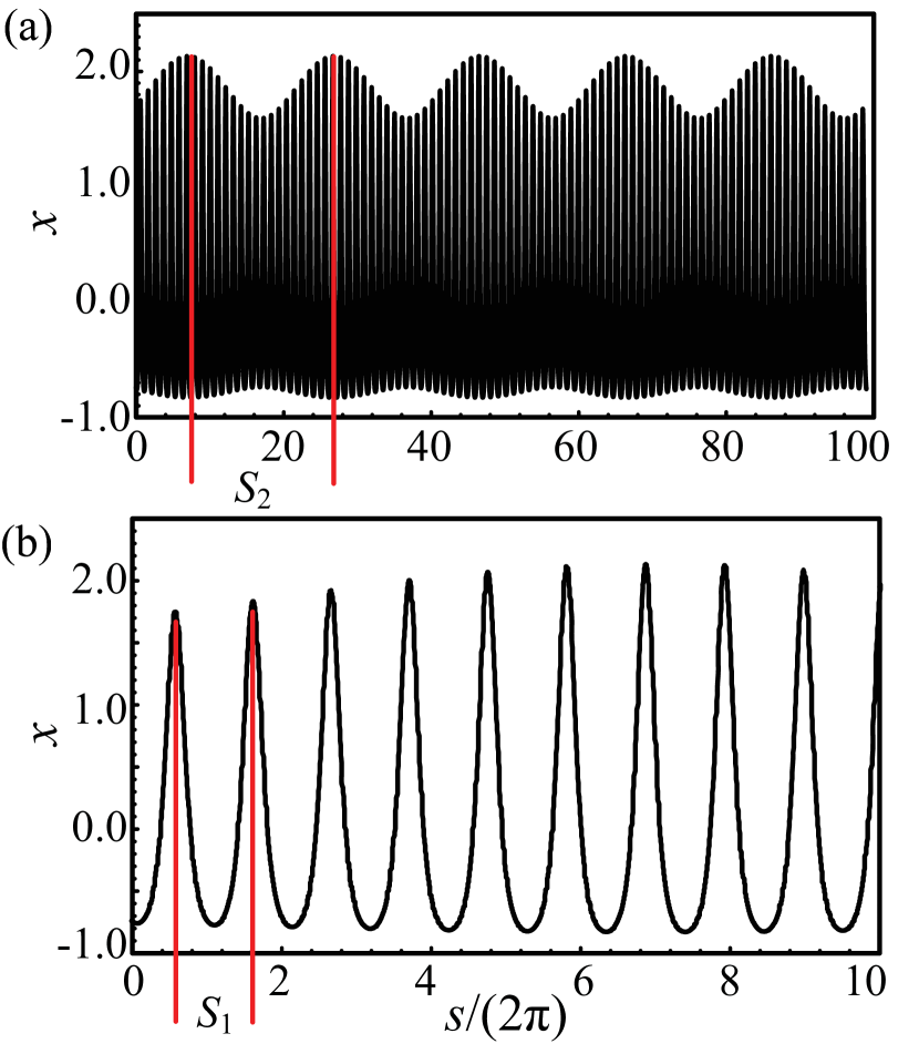
Figure 1: Numerically obtained quasiperiodic oscillations. Both (a) and (b), show deviation $x$ of the intensity $I$ from its steady state value in different time scales for $\eta=0.025,$ $\theta=9.9\times 2\pi$ and $\varepsilon=0$. The two periods are $S_{1}=1.03$ and $S_{2}=19.81$.

III Weakly nonlinear analysis

The fact that $\eta_{SB}$ $\rightarrow 0$ as $\theta\rightarrow\infty$ motivates a weakly nonlinear analysis where

$$\delta\equiv 1/(2n)$$ (7)

will be considered as a small parameter, and

$$\eta=\delta b,\text{ }$$ (8)

where $b=\mathcal{O}(1).$ Furthermore, we scale the small parameter $\varepsilon$ in a similar way as

$$\varepsilon=\delta c,\text{ }$$ (9)

where $c=\mathcal{O}(1)$. The perturbation analysis is detailed in the Appendix B. We find that

$$x=\delta^{1/2}(iA(r)\exp(is)+c.c.)+\mathcal{O}(\delta),$$ (10)

where $r\equiv\delta s$ is a slow time variable. The complex amplitude $A(r)$ satisfies the following equation

$$2i\frac{dA}{dr}=\frac{1}{3}A^{2}A^{\ast}-Ab+bA(r-\delta\theta)\exp(-i\theta)$$

$$-ic(1+2P)A$$ , (11)

which we now propose to explore. Eq. (11) was previously derived (Eq. (19) in Gavrielides et al. (2000)). Here, we concentrate on the quasiperiodic oscillations of the laser equations which now correspond to periodic solutions of Eq. (11).  Of particular interest is the period of the oscillations.

III.1 No damping rate of the RO oscillations and perfect resonance

We first examine the simple case $c=0$ and $\theta=\theta_{n}=2n\pi$.  Introducing the decomposition $A=R\exp(i\phi)$ into Eq. (11), we obtain from the real and imaginary parts

$$2R^{\prime} =bR(r-\pi)\sin(\phi(r-\pi)-\phi),$$ (12)

$$2\phi^{\prime} =-\frac{R^{2}}{3}+b-b\frac{R(r-\pi)}{R}\cos(\phi(r-\pi)-\phi),$$ (13)

where prime now means differentiation with respect to $r$.

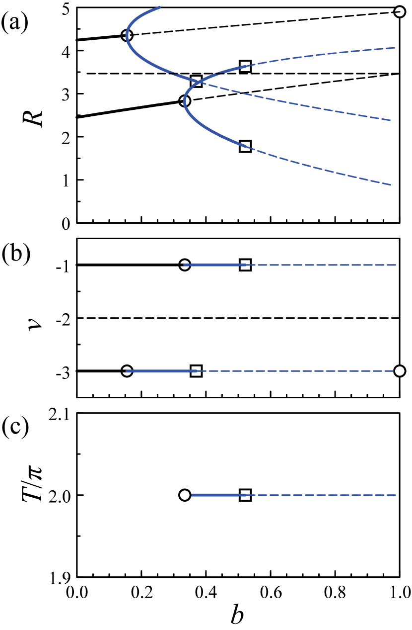
Figure 2: Bifurcation diagram of the steady state (black) and periodic (blue) solutions of the slow time amplitude equations (12) and (13). We use the decomposion $A=R\exp(i\phi)$, where $\phi=\nu r$ is introduced in the text. Figure (a) represents the extrema of $R$ as a function of the scaled feedback strength $b$ for $\theta=2n\pi.$ They have been obtained by using the numerical continuation method Engelborghs et al. (2002). Full and broken lines are stable and unstable solutions, respectively.  The figure shows two stable branches of constant $R$ solutions emerging from $b=0.$ Circles are Hopf bifurcation points $b_{H}$ leading to stable oscillations up to new bifurcation points $b_{PD}$ denoted by squares.  Figure (b) represents the slow time frequency correction $\nu$ for the first three branches of steady states namely, $\nu=-1,-2,$ and $-3$. Figure (c) shows the period of the periodic solution bifurcating from $R=\sqrt{6(1+b)}$, $\nu=-1$ at $b_{H}=1/3$. The period remains constant as $b$ further increases from $b_{H}.$

These equations admit constant $R$ solutions with phase $\phi=\nu r$. In terms of time $s$, the frequency of the basic RO oscillations in units of the the orginal time $s$ now is $1+\delta\nu.\$Fig. 2(a) shows two stable and one unstable branch emerging from $b=0$. The two stable branches depend on $b$ and are given by (see Appendix B)

$$R=\sqrt{6(b-\nu)}\text{, and }\nu=-1,-3,$$ (14)

while the unstable branch is independent of $b$ and admit the value

$$R=\sqrt{12}.$$ (15)

The Hopf bifurcation point $b_{H}$ of Solution (14) with $\nu=-1$ is determined analytically for arbitrary $\theta$ in the Appendix B. If $\theta=\theta_{n}$, it is located at

$$b_{H}=\frac{1}{3},$$ (16)

and agrees with the numerical estimate in Fig. 2. The Hopf bifurcation frequency in units of time $r$ is equal to $1$ meaning that the period of the oscillations at the bifurcation point equals $T=2\pi.$ Fig. 2(c) shows the period of the oscillations as their amplitude increases ($b>$ $b_{H}).$ Surprisingly, it remains close to $2\pi$. This branch of periodic solutions changes stability at a new bifurcation point $b_{PD}$ (squares in Fig. 2(a)). Simulations indicate that it corresponds to a period doubling bifurcation.

III.2 Non-zero RO damping rate and near resonant conditions

We now consider the case $c\neq 0$ and $\theta$ close, but different from $\theta_{n}=$ $2n\pi.\$Introducing the decomposition $A=R\exp(i\phi)$ into Eq. (11), we obtain

$$2R^{\prime} =bR(r-\delta\theta)\sin(-\theta+\phi(r-\delta\theta)-\phi)-c(1+2P)R,$$ (17)

$$2\phi^{\prime} =-\frac{1}{3}R^{2}+b-b\frac{R(r-\delta\theta)}{R}\cos(-\theta+\phi(r-\delta\theta)-\phi),$$ (18)

where prime means differentiation with respect to $r$.

The solutions with $R=\text{const}$ and $\phi=\nu r,$ in parametric form, are given by ($\nu$ is the parameter)

$$b =-\frac{c(1+2P)}{\sin(\theta+\nu\delta\theta)},$$ (19)

$$R^{2} =3\left[-2\nu+b-b\cos(\theta+\nu\delta\theta)\right]\geq 0.$$ (20)

Figure 3 shows the bifurcation diagram for the extrema of $R$ as a function of $b.$ The figure exhibits two Hopf bifurcations from two distinct branches of constant $R$ solutions (two left circles in Fig. 3). Both bifurcations are leading to stable oscillations which become unstable at new bifurcation points (squares in Fig. 3).

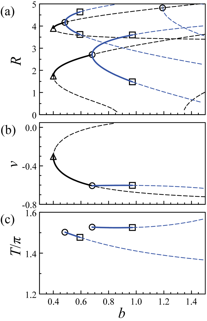
Figure 3: Bifurcation diagram of the steady state and periodic solutions of Eqs. (17) and (18). Scaled decomposion $A=R\exp(i\phi)$, where $\phi=\nu r$ is introduced in the text. Figure (a) represents the extrema of $R$ as a function of the scaled feedback strength $b.\$The parameter values are $\theta=9.9\times 2\pi$ and $P=0.5.\$ $\theta$ is close to $\theta_{n}=2n\pi$ with $n=10.$ This then implies that $\delta=1/(2n)=1/20,$ $c=0.2$ if $\varepsilon=0.01$, and $\delta\theta=0.99\pi.$ They have been obtained by using the numerical continuation method Engelborghs et al. (2002). The figure shows two stable branches of constant $R$ solutions emerging from limit points (triangles). The other notations and colors are the same as in Fig. 2. Figure (b) represents the slow time frequency correction $\nu$ for the first branch. Figure (c) shows the period of the periodic solutions bifurcating from the two branches of constant $R$ solutions. Note that only the first Hopf bifurcation leads to a constant period as we increase $b$.

Simulations of the amplitude Eq. (11), reformulated in terms of $A=u+iv$, for long intervals of time indicate that the secondary bifurcation is a period doubling bifurcation and is followed by higher order instabilities (Fig. 4; only the bifurcation diagram corresponding to the first Hopf bifurcation branch is shown for clarity).

Figure 4: Numerical bifurcation diagram of the extrema of $R$ as a function of the scaled feedback strength $b$ for $\theta=2n\pi.$ Scaled decomposion $A=R\exp(i\phi)$, where $\phi=\nu r$ is introduced in the text. Long-time simulations were obtained from Eq. (11) reformulated in terms of the real and imaginary parts of $A$. The original values of the parameters are: $\varepsilon=10^{-2},$ $\theta=9.9\times 2\pi,$ and $P=0.5.\$ $\theta$ is close to $\theta_{n}=2n\pi$ with $n=10$ implifying $\delta=1/20,$ $c=0.2$, and $\delta\theta=0.99\pi.$ The red lines are the constant $R$ solutions given by Eqs. (19) and (20). 

We observe that the period of the first Hopf bifurcation branch remains constant as the amplitude of the oscillations increases. The period is no more nearly equal to $2\pi$ but is given by

$$T/\pi=1.525\text{ }(b_{H}<b<b_{PD}).$$ (21)

Accurate two parameter studies for $\theta$ close to $\theta~{}=~{}10\times 2\pi$ have been determined by using a continuation method, and are shown in Fig. 5. In Fig. 5(a) the stable oscillations of Eqs. (17) and (18) are bounded in the $b$ versus $\theta$ plane by Hopf bifurcation lines (solid), period-doubling bifurcation lines (dashed), and torus bifurcation lines (dotted). The torus bifurcation leads to quasiperiodic oscillations. In this figure, the red delimits the domain of stable periodic solutions connected to the first steady state branch that bifurcates from zero if $\theta_{c1}<\theta<\theta_{c2}$ ($\theta_{c1}=8.94\times 2\pi$ and $\theta_{c2}=9.93\times 2\pi$, see Fig. 10 of the Appendix B for the primary Hopf bifurcation lines). At the double Hopf bifurcation point $\theta=\theta_{c2}$ two distinct steady state branches emerge from zero at the same value of $b$. If $\theta>\theta_{c2}$, a new steady state branch becomes the first to appear from zero. The domain of stable oscillations for this new branch is indicated in blue in Fig. 5. A similar bifurcation scenario where a new steady-state branch becomes first occurs if $\theta<\theta_{c1}$. Its domain of stable oscillations is shown in orange in Fig. 5.

Figure 5(b) shows the period as a function of $\theta$. At the intersections of the full and dashed lines, the period is constant for the whole range of $b$ where the corresponding periodic solutions are stable. The bifurcation diagram shown in Fig. 3 is for $\theta=9.9\times 2\pi$ which corresponds to the intersection point of the red lines in Fig. 5. The periodic solution which stability domain is bounded by the red area in Fig. 5 exhibits the constant period as shown by the upper line in Fig. 3(c).

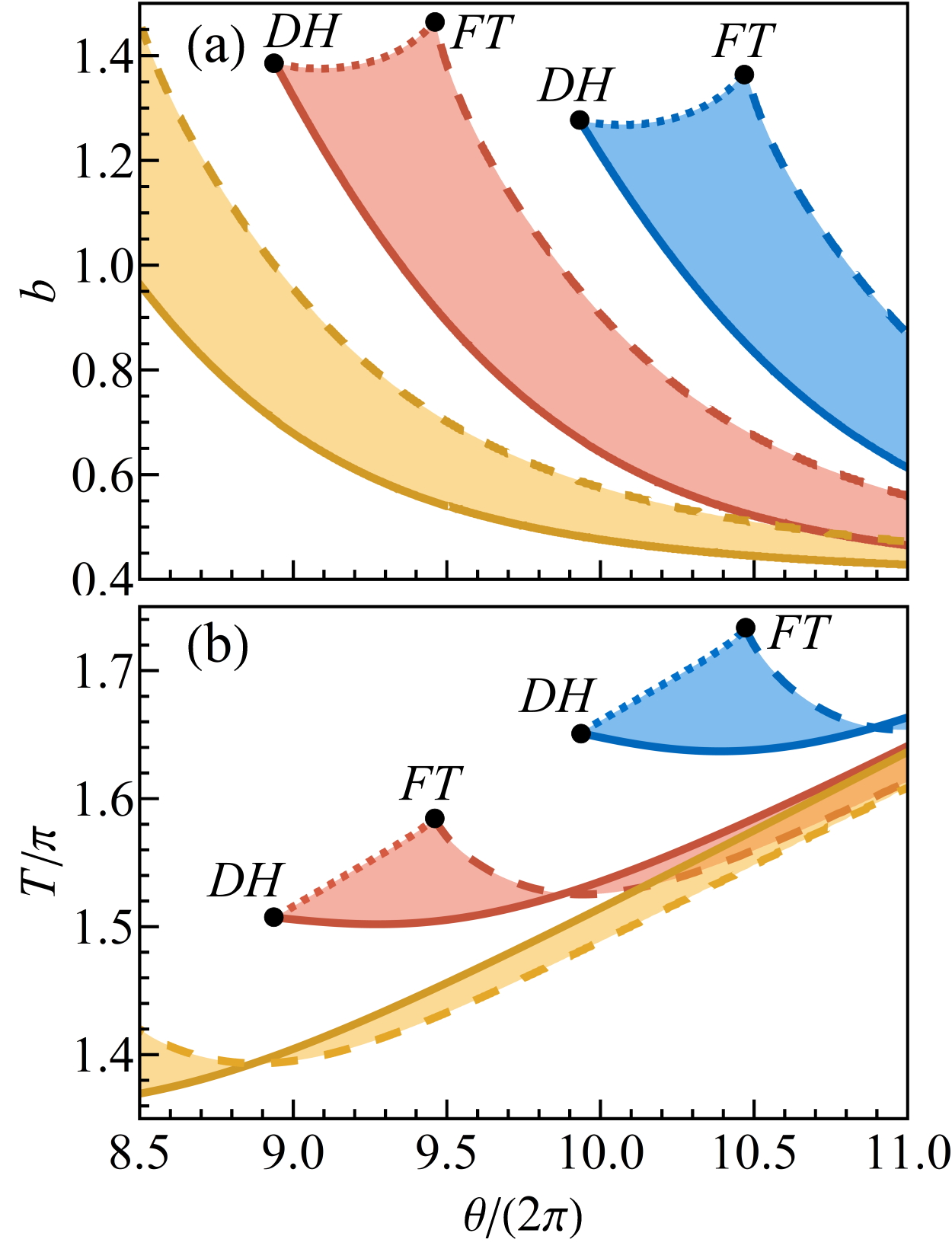
Figure 5: Figure (a): domains of stable periodic solutions of Eqs. (17) and (18) in the $(\theta,b)$ plane; figure (b): corresponding oscillation periods. Solid lines are the Hopf bifurcation lines leading to the periodic solutions. Dashed (dotted) lines stand for period-doubling (torus) bifurcation lines. The colored areas delimit the domains of stable oscillations. The red domain is for the periodic solutions that bifurcate from the first steady state branch if $\theta_{c1}<\theta<\theta_{c2}$. The other colors correspond to periodic solutions bifurcating from other neighbouring branches of steady states. The black dots denote codimension-2 bifurcations located at the cusps: $DH$ are the double Hopf bifurcation points of the zero solution at $\theta_{c1}$ and $\theta_{c2}$; $FT$ are the flip-torus bifurcation points of the periodic solutions. The parameters are the same as in Fig. 3.

IV Constant period

In this section, we reconsider Eqs. (12) and (13), which are written for the scaled deviation of intensity $I$ from their steady state values and plan to explain why the period remains constant as we pass the Hopf bifurcation point. Our approach is similar to the analysis of time periodic square-wave solutions of scalar delay differential equations (DDEs). In Eqs. (12) and (13), the delay equals $\pi$ and will be treated as a large parameter.

We first introduce the variables $R_{j}$ and $\phi_{j}$ $(j=0,1,2)$ defined by

$$R_{0} \equiv R(r-\frac{\pi}{2}),\text{ }R_{1}\equiv R(r),\text{ }R_{2}\equiv R(r+\frac{\pi}{2}),$$ (22)

$$\phi_{0} \equiv\phi(r-\frac{\pi}{2}),\text{ }\phi_{1}\equiv\phi(r),\text{ and }\phi_{2}\equiv\phi(r+\frac{\pi}{2}).$$ (23)

We next consider two successive iterations of Eqs. (12) and (13), namely

$$2R_{1}^{\prime} =bR_{0}\sin(\phi_{0}-\phi_{1}),$$ (24)

$$2R_{2}^{\prime} =bR_{1}\sin(\phi_{1}-\phi_{2}),$$ (25)

$$2\phi_{1}^{\prime} =-\frac{R_{1}^{2}}{3}+b-b\frac{R_{0}}{R_{1}}\cos(\phi_{0}-\phi_{1}),$$ (26)

$$2\phi_{2}^{\prime} =-\frac{R_{2}^{2}}{3}+b-b\frac{R_{1}}{R_{2}}\cos(\phi_{1}-\phi_{2}).$$ (27)

The numerical simulations indicate that the period $p$ of the oscillations is close to $2\pi.$ We therefore write

$$p=2\pi+\alpha\text{ }$$ (28)

where the correction $\alpha$ is assumed small compared to $2\pi.\$With (28), the variables $R_{0}$ and $R_{1}$ are expanded as

$$R_{0} \equiv R(r-\pi)=R(r-\frac{p}{2}+\frac{\alpha}{2})=R(r-\frac{p}{2})+\mathcal{O}(\alpha),$$ (29)

$$R_{2} \equiv R(r+\pi)=R(r+\frac{p}{2}-\frac{\alpha}{2})=R(r+\frac{p}{2})+\mathcal{O}(\alpha).$$ (30)

The periodicity condition now implies that

$$R_{2}=R_{0}$$ (31)

in first approximation. Similarly

$$\phi_{2}=\phi_{0}.$$ (32)

With (31) and (32), Eqs. (24) and (27) reduce to four ordinary differential equations

$$2R_{1}^{\prime} =bR_{0}\sin(\phi_{0}-\phi_{1}),$$ (33)

$$2R_{0}^{\prime} =bR_{1}\sin(\phi_{1}-\phi_{0}),$$ (34)

$$2\phi_{1}^{\prime} =-\frac{R_{1}^{2}}{3}+b-b\frac{R_{0}}{R_{1}}\cos(\phi_{0}-\phi_{1}),$$ (35)

$$2\phi_{0}^{\prime} =-\frac{R_{0}^{2}}{3}+b-b\frac{R_{1}}{R_{0}}\cos(\phi_{1}-\phi_{0}).$$ (36)

Introducing $\Phi\equiv\phi_{1}-\phi_{0},$ we may eliminate one equation

$$2R_{1}^{\prime} =-bR_{0}\sin(\Phi),$$ (37)

$$2R_{0}^{\prime} =bR_{1}\sin(\Phi),$$ (38)

$$2\Phi^{\prime} =-\frac{R_{1}^{2}-R_{0}^{2}}{3}-b(\frac{R_{0}}{R_{1}}-\frac{R_{1}}{R_{0}})\cos(\Phi).$$ (39)

From Eqs. (37) and (38), we note a conservation relation given by

$$R_{0}^{2}+R_{1}^{2}=E,$$ (40)

where $E$ is a positive constant. Solving numerically Eqs. (12) and (13) for $b=0.5$, we find that $E(r)\equiv R^{2}(r)+R^{2}(r-\pi)$ oscillates close to a constant:

$$E(r)=16.32\pm 0.02.$$ (41)

Using $R_{1}=\sqrt{E-R_{0}^{2}},$ we may further eliminate one equation and obtain

$$2R_{0}^{\prime} =b\sqrt{E-R_{0}^{2}}\sin(\Phi),$$ (42)

$$2\Phi^{\prime} =(2R_{0}^{2}-E)\left[\frac{1}{3}-\frac{b}{R_{0}\sqrt{E-R_{0}^{2}}}\cos(\Phi)\right].$$ (43)

One steady state is given by

$$\Phi=\pi\text{ and }R_{0}^{2}=E/2.$$ (44)

From the linearized equation, we determine the characteristic equation for the growth rate $\lambda$

$$4\left[\lambda^{2}+b(\frac{R_{0}^{2}}{3}+b)\right]=0.$$ (45)

The $2\pi$ periodicity condition requires that $\lambda=i$ and (45) simplifies as

$$-1+b(\frac{R_{0}^{2}}{3}+b)=0.$$ (46)

We have verified that the expression of the steady state Eq. (14) and its bifurcation point Eq. (16) identically satisfy Eq. (46). We conclude that Eqs. (42) and (43) correctly predict the previously determined Hopf bifurcation point. By dividing Eqs. (42) and (43), we obtain a first order equation for $\cos(\Phi)$ as a function of $R_{0}.$ This equation can be integrated and its solution exhibits a new constant of integration $C$.

In summary, the analysis of the leading order equations indicates that the amplitude and period of the oscillations depend on the values of two unknown constants $E$ and $C$. Therefore, we need to explore higher order problems and formulate two solvability conditions with respect to $E$ and $C$. The higher order problems will exhibit the correction of the frequency $\alpha$ and we need the third condition. It is provided by the periodicity condition of $R_{0}$ and $\phi_{0}.$ The higher order analysis is beyond the scope of this paper. Our main objective was the derivation of the ODEs Eqs. (42) and (43) from the original DDE problem Eqs. (12) and (13). In order to substantiate our analysis, we have arbitrary fixed the parameters $E$ and $C$ and solved Eqs. (42) and (43) for $b=0.5$ with the goal of finding the best fit to the numerical solution of the full Eqs. (12) and (13). The value of $E=16.32$ is motivated by Eq. (41), and the value of $C$ is determined by choosing the initial conditions. Since the maximum of $R$ appears when $\Phi=\pi,$ we consider $\Phi(0)=\pi$ and only modify $R(0)$ so that the period of the oscillations equals $2\pi.$ Fig. 6 compares the time traces of the original DDEs and reduced ODEs. The agreement is excellent.

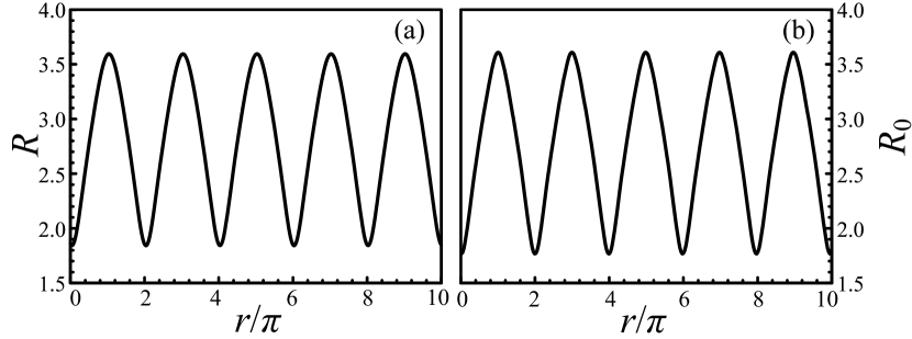
Figure 6: (a): Numerical solution of the DDEs (12) and (13). Scaled decomposion $A=R\exp(i\phi)$, where $\phi=\nu r$ is introduced in the text. (b): Numerical solution of the ODEs (42) and (43) with $E=16.32$, and initial conditions $R_{0}(0)=3.61$, $\Phi(0)=\pi.$ Parameter $b=0.5.$ 

V Experiments

Our mathematical analysis considered the rate equations for a semiconductor laser subject to a delayed optoelectronic feedback and predicted a resonance locking effect between the RO laser frequency and a much lower frequency appearing through a secondary bifurcation mechanism. The latter is inversely proportional to the delay and exhibits a value that remains nearly constant as we increase the control parameter. This unexpected property from a bifurcation theory point of view motivates our experiments.

The device used for the experiments is a single mode edge-emitting distributed feedback (DFB) p-doped InAs/InP QDash laser with a cavity length of  500 $\mu$m, operating at 1550 nm. The DFB laser used has an active region consisting of a stack of six layers of InAs quantum dashes, each layer being embedded within an InGaAsP quantum well and separated by InGaAsP barriers, AR/AR coated facets and a threshold current of 33 mA at room temperature. The side mode suppression ratio was in excess of 40 dB in the whole range of pumping used in the experiments.

The experimental setup is shown in Fig. 7. The OE feedback consists of three stages. The first stage corresponds to 35 cm of free space optical path which provides $\sim$1.17 ns delay. This free space path includes a collimating lens (CL), an optical isolator (OI) that prevents back reflections into the laser, a linear polarizer (LP) and an objective lens (OL) that focuses the light onto an optical fiber. The second stage corresponds to 35 cm of optical patch cable, providing $\sim$1.73 ns delay, and leading to a high-bandwidth photodetector (12 GHz Newfocus 1544-B). The third stage is the electronic path which starts with the photodetector and whose output is amplified before being fed back to the laser. The amplification is implemented by cascading a 18 dB amplifier with 20 GHz bandwidth (Newport 1422-LF) and a 30 dB amplifier with 30 GHz bandwidth (Microsemi UA0L30VM). The delay of the electronic path, which also includes 70 cm of microwave coaxial cable and a high frequency splitter (Mini-circuits ZX-10-2-183-S+), is measured to be $\sim$5.67 ns. The total delay of the OE feedback loop is then estimated as $1.17+1.73+5.67=8.57$ ns ($\pm 0.20$ ns). The experimental effective feedback level $\eta$ is here a relative measure of the feedback strength and cannot be directly compared to the theoretical $\eta$ used in our analysis. The parameter $\eta$ is controlled through the linear polarizer (LP); it is affected by the responsivity of the photodetector and the gain of the two amplification stages. Conventionally, $\eta=1$ corresponds to full transmission by the linear polarizer. Rotating the LP allows a nonlinear control of the feedback level, since the attenuation introduced varies as the cosine square of the angle between the LP and the direction of polarization of the laser. Finally, a 50/50 RF splitter (18 GHz) was used to simultaneously feed the laser back and to monitor the signal with the oscilloscope (12 GHz bandwidth, Agilent DSO80804B). The splitter output used for feedback was directly added to the DC bias current of the laser through a bias tee (26.5 GHz Marki BT-0026).

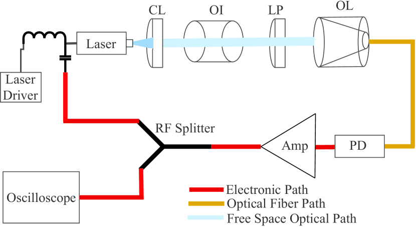
Figure 7: Experimental arrangement of a laser diode subjected to optoelectronic feedback. The optical intensity is photodetected, amplified and added to the DC bias current of the laser diode. An oscilloscope monitors the amplifier output. Various feedback levels are obtained by rotating the linear polarizer in the free space optical path. CL – collimating lens, OI – optical isolator, LP – linear polarizer, OL – objective lens, PD – photodetector.

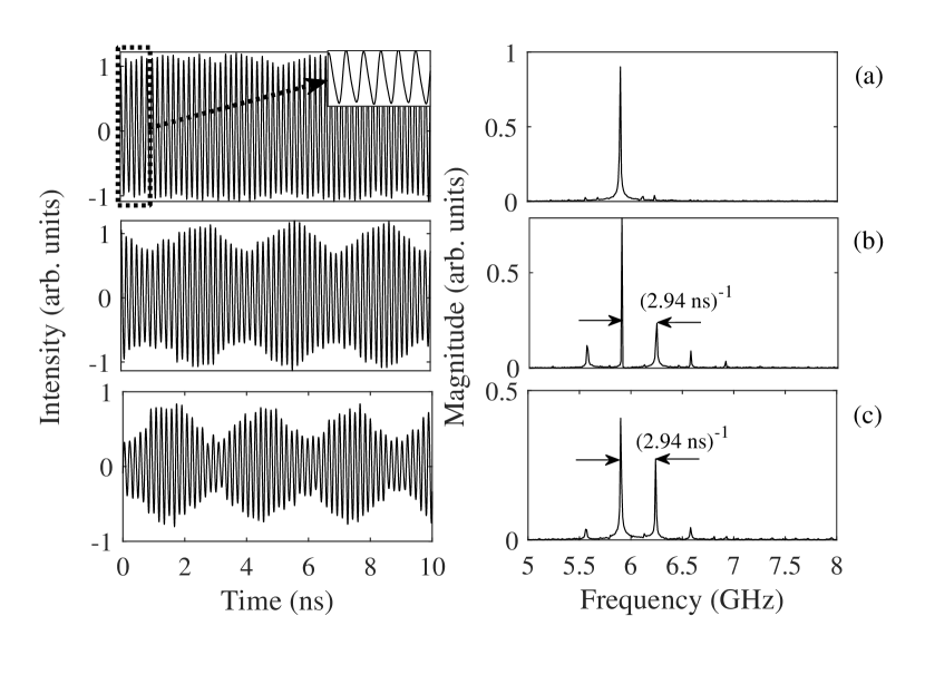
Figure 8: Optical intensity (left column) and RF spectra (right column) at 68 mA of pump current for various feedback levels: (a) $\eta=0.56$, (b) $\eta=0.58$, (c) $\eta=0.59$.

The free running laser operates at 68 mA pump current, providing 4 mW output power. For low feedback strength $\eta$, the laser output remains stable (apart from noise). Using LP as a variable optical attenuator in the optical path, the feedback level $\eta$ was increased until cw operation was lost , and a Hopf bifurcation appears. The latter leads to sustained relaxation oscillations. A regular, nearly-sinusoidal 5.9 GHz oscillation is obtained at $\eta=0.56$ (see Fig. 8(a)). The experimental feedback strength $\eta$ is in arbitrary units, but is proportional to the current fed back into the injection terminals. When $\eta=0.56$, the fed back current is approximately 15% the injection current.

As the level of feedback $\eta$ is further increased, the generation of sidebands in the RF spectra, spaced at approximately $\sim$0.34 GHz (slow period $\sim$2.94 ns), was observed indicating a new bifurcation transition. This bifurcation arises at $\eta=0.58$ as the output displays quasiperiodic intensity traces slightly affected by the noise in the system (Fig. 8(b)). Further increase of the feedback sufficiently affects the amplitude of the slow envelope and its shape. The slow period, however, remains constant for the whole feedback range. It is worth noting here that the slow period of the quasiperiodic oscillations $\sim$2.94 ns is nearly three times smaller than that of the $\sim$8.57 ns as estimated delay time.

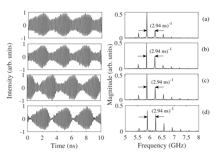
Figure 9: Optical intensities (left) and RF spectra (right) for a range of pump currents $J$ and feedback levels: (a) $J$ = 64 mA, $\eta=0.56$, (b) $J$ = 65 mA, $\eta=0.57$, (c) $J$ = 66 mA, $\eta=0.58$, (d) $J$ = 67 mA, $\eta=0.59$.

The effective time scales measured in the experiment result from $1:17$ resonance between the low $\sim$0.34 GHz and $large$ $\sim$5.9 GHz frequencies of the quasiperiodic oscillations. In order to verify the model assumptions about the high-order resonant effect, we have also varied the pump current which led to noticeable changes in the shape and amplitude of the quasiperiodic oscillations. However, as shown in Fig. 9, the fast and slow fundamental frequencies were not affected as they remained fixed (to $\sim$5.9 GHz and $\sim$0.34 GHz, respectively) for the whole range of the control parameters.

VI Conclusion

In this paper, we considered a semiconductor laser with delayed optoelectronic feedback. We prove, analytically, and demonstrate, numerically and experimentally, that resonant locking between two fundamental laser frequencies, namely, $f_{RO}$ and $f_{delay}$, allows their ratio to remain constant despite growing amplitude oscillations. Understanding of SLs with optoelectronic feedback is a relatively undeveloped field compared with purely optical feedback; however, understanding these effects is important from the viewpoints of stabilizing desired dynamics, gaining insight into undesirable effects of feedback, as well as to explore novel nonlinear dynamical effects.

Appendix A Asymptotic methods based on the large delay limit

Asymptotic methods for delay differential equations exhibiting a large delay take advantage of the distinct time scales in the physical problem. In particular, Hopf bifurcation instabilities have been studied in detail, and the predictions of their amplitude equations have been successfully tested on several case studies. It is worth emphasizing that there exist two distinct limits that provide valuable information in their domains of validity. We illustrate these different approaches by considering Minorsky equation for a weakly damped and weakly nonlinear oscillator Pinney (1958):

$$y^{\prime\prime}+\varepsilon y^{\prime}+y=-\varepsilon dy^{\prime}(t-\tau)+\varepsilon cy^{\prime^{3}}(t-\tau),$$ (47)

where $\varepsilon$ is small and $\tau$ is large. Assuming discrete values $\tau=(1+2n)\pi$, where $n$ is a large integer, allows the derivation of an amplitude equation in  its simplest mathematical form. Specifically, we scale the delay $\tau$ with respect to $\varepsilon$ as $\tau=\varepsilon^{-1}\tau_{1}$, and find that the first Hopf bifurcation of Eq. (47) leads to the solution Erneux (2009):

$$y=A(s)\exp(it)+c.c.+\mathcal{O}(\varepsilon),$$ (48)

where the complex amplitude $A$ depends on the slow time variable $s=\varepsilon t$. It satisfies the slow time equation

$$A^{\prime}=\frac{1}{2}\left[-A+dA(s-s_{1})-3cA^{3}(s-s_{1})\right],$$ (49)

where prime now means differentiation with respect to time $s$, and $s_{1}\equiv\varepsilon\tau_{1}=\mathcal{O}(1)$ or larger. This equation is analyzed in Erneux (2009) and reveals a cascade of primary and secondary bifurcations.

If we now analyze the stability of the zero solution of Eq. (49) using $d$ as the bifurcation parameter, we observe that the first Hopf bifurcation point $d_{H}\rightarrow 1$ as $s_{1}\rightarrow\infty.\$ The nature of the bifurcation corresponds to an uniform instability according to Ref. Yanchuk and Giacomelli (2017). Introducing the small parameter $\delta\equiv s_{1}^{-1}\ll 1,$ and expanding $d$ as $d=1+\delta^{2}d_{2}+...$, we may construct a small amplitude solution of the form Wolfrum and Yanchuk (2006); Yanchuk and Giacomelli (2017)

$$A=\delta u(x,\nu)+\mathcal{O}(\delta^{2})$$ (50)

where $x\equiv\varepsilon(1+\varepsilon/a+\varepsilon^{2}/a^{2})t$and $\nu\equiv\delta^{3}t$ are called pseudo-space and pseudo-time, respectively Yanchuk and Giacomelli (2017). The function $u$satisfies the Ginzburg-Landau (GL) equation

$$u_{\nu}=2u_{xx}+b_{2}u-3cu^{3},$$ (51)

$$u(x-1)=u(x).$$ (52)

An obvious question is how to relate the small parameters $\delta\$and $\varepsilon.$ By considering $\delta=\varepsilon,$or equivalently, $\tau=\varepsilon^{-2}\tau_{2},$ and seeking a solution of Eq. (47) in powers of $\varepsilon$ leads to Eqs. (51) and (52) Erneux (2009).

In summary, the limit $\tau=\varepsilon^{-1}\tau_{1}$ is leading to a slow time DDE for $\mathcal{O}(1)$ amplitude multi-periodic solutions. On the other hand the limit, $\tau=\varepsilon^{-2}\tau_{2}$ is leading to a GL equation for small amplitude solutions. The latter allows to relate our DDE problem to spatially extended systems Arecchi et al. (1992); Grigorieva et al. (1999). Here, we consider the first limit because it quantitatively describes the instabilities observed numerically, and allows us to analyze high-order locking phenomena, manifested by the resonance between the multiple timescales in the laser subject to the optoelectronic feedback.

Appendix B The laser amplitude equation and its solutions

B.1 Hopf bifurcations

We consider the rate equations for a semiconductor laser subject to a delayed optoelectronic feedback Erneux and Glorieux (2010). In dimensionless form, they are given by

$$I^{\prime} = 2NI,$$ (53)

$$TN^{\prime} = P+\eta I(t-\tau)-N-(1+2N)I,$$ (54)

where $I$ is the intensity of the laser field and $N$ is the carrier density. $P\sim 1$ is the value of the pump parameter above threshold in the absence of feedback $(\eta=0).$ $T\sim 10^{3}$ is the ratio of the carrier and photon lifetimes. $\eta<1$ and $\tau\sim 10^{3}$ are the gain and the delay of the optoelectronic feedback, respectively. By introducing the new variables $x$, $y$, and $s$ defined by

$$N\equiv\frac{\omega}{2}x,\text{ }I\equiv P(1+y)\text{, and }s\equiv\omega t$$ (55)

where

$$\omega\equiv\sqrt{\frac{2P}{T}}$$ (56)

is the (angular) RO frequency, we may eliminate the large $T$ parameter multiplying the left hand side of Eq. (54). Specifically, we obtain the following equations for $y$ and $x$

$$y^{\prime} = x(1+y),$$ (57)

$$x^{\prime} = -y+\eta(1+y(s-\theta))-\varepsilon x\left[1+2P(1+y)\right],$$ (58)

where

$$\varepsilon\equiv\frac{\omega}{2P}<<1\text{, and }\theta=\omega\tau.$$ (59)

The non-zero intensity steady state is

$$(x,y)=(0,\frac{\eta}{1-\eta}).$$ (60)

From the linearized equations, we determine the characteristic equation for the growth rate $\lambda$. We find

$$\lambda^{2}+\varepsilon\lambda(1+\frac{2P}{1-\eta})+1-\frac{\eta}{1-\eta}(\exp(-\lambda\theta)-1)=0.$$ (61)

The stability domains in the $(\eta,\theta)$ parameter space are bounded by Hopf bifurcation lines. Introducing $\lambda=i\sigma$ into Eq. (61), we obtain the Hopf conditions relating $\eta$  and $\sigma.$ They are given by

$$-\sigma^{2}+1-\frac{\eta}{1-\eta}(\cos(\sigma\theta)-1) = 0,$$ (62)

$$\sigma\varepsilon(1+\frac{2P}{1-\eta})+\frac{\eta}{1-\eta}\sin(\sigma\theta) = 0.$$ (63)

Figure 10 shows the stability domains for $\varepsilon=0.01$ and for $\varepsilon=0$ $(8.5<\theta/(2\pi)<11)$. As $\varepsilon\rightarrow 0,$ the Hopf stability boundaries are shrinking to straight lines. An analysis of Eq. (61) with $\varepsilon=0$ and $\eta\rightarrow 0$ leads to the stability condition

$$\sin(\theta)>0\text{ }(\varepsilon=0,\eta\rightarrow 0).$$ (64)

This explains the sequential change of stability along the $\eta=0$ axis in Fig. 10(b).

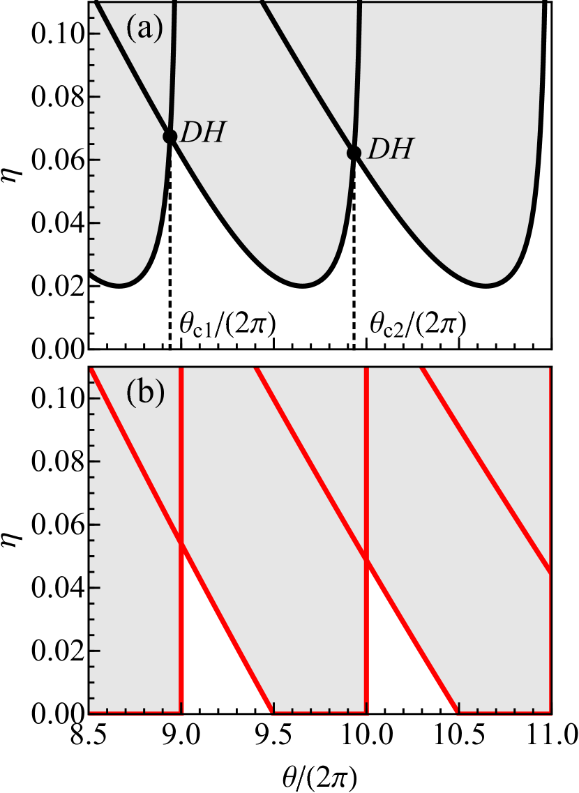
Figure 10: (a) Primary Hopf bifurcation lines in the interval $8.5<\theta/(2\pi)<11$ as we increase $\eta$ from zero $(\varepsilon=0.01$ and $P=0.5).$ At double Hopf points $DH$ (black dots), $\theta_{c1}=8.94\times 2\pi$ and $\theta_{c2}=9.93\times 2\pi$, two distinct bifurcation lines are crossing. (b) Primary Hopf bifurcation lines if $\varepsilon=0.$ They are given by (68) and (69) with $n=9,$ $10,$ $11$, and by (67). The shaded (white) areas in (a) and (b) denote the zones of unstable (stable) steady state solutions.

If $\varepsilon=0,$ Eqs. (62) and (63) are easily solved. We find three families of solutions given by

(1): $$\sigma\theta=2n\pi\text{ }(n=1,...)\text{, and }\sigma=1,$$ (65)

(2): $$\sigma\theta=(2n+1)\pi\text{ }(n=0,\text{ }1,...)$$

$$\text{ and }\sigma=\sqrt{1+\frac{2\eta}{1-\eta}},$$ (66)

(3): $$\eta=0\text{, and }\sigma=1.$$ (67)

The three cases provide the vertical lines in Fig. 10(b):

$$\text{(1): }\theta=2n\pi\text{ }(n=1,...),$$ (68)

the lines

$$\text{(2): }\theta=\frac{(2n+1)\pi}{\sqrt{1+\frac{2\eta}{1-\eta}}}\text{ }(n=0,\text{ }1,...),$$ (69)

and the horizontal line (67).

B.2 Perturbation analysis

We next consider values of $\theta$ close to

$$\theta_{n}\equiv 2n\pi$$ (70)

and wonder if a secondary bifurcation is possible. Numerical simulations of Eqs. (57) and (58) suggest that such bifurcation appears at a value of $\eta$ satisfying the scaling law $\eta\sim n^{-1}$ for large $n$. It motivates a weakly nonlinear analysis where

$$\delta\equiv 1/(2n)$$ (71)

will be considered as a small parameter. To facilitate the algebra, it will be convenient to eliminate $x$ and formulate a second order delay differential equation for $u\equiv\ln(1+y)$ only. From Eqs. (57) and (58), we find that $u$ satisfies

$$u^{\prime\prime}= 1-\exp(u)+\eta\exp(u(s-\theta))$$

$$-\varepsilon u^{\prime}(1+2P\exp(u)).$$ (72)

We are now ready to start our analysis. We introduce the new control parameters $b=\mathcal{O}(1)$ and $c=\mathcal{O}(1)$ defined as

$$b\equiv\eta\delta^{-1},\text{ }c\equiv\varepsilon\delta^{-1},$$ (73)

and seek a solution depending on two distinct time variables of the form

$$u=\delta^{1/2}u_{1}(s,r)+\delta u_{2}(s,r)+...,$$ (74)

where $r\equiv\delta s$ is defined as a slow time variable. The $\delta^{1/2}$ power series in (74) and the scaling of $\eta$, and $r$ result from the fact that the desired amplitude equation only appears at the third order of the perturbation analysis. The assumption of two independent time scales implies the chain rule

$$u^{\prime\prime}=u_{ss}+2\delta u_{sr}+\delta^{2}u_{rr},$$ (75)

where the subscripts $s$ and $r$ mean partial derivatives with respect to $s$ and $r$. We also note that

$$u(s-\theta)=u(s-\theta,r-\delta\theta).$$ (76)

Introducing (73)–(76) into Eq. (72) and equating to zero the coefficients of each power $\delta^{1/2}$ lead to a sequence of linear problems for the unknown functions $u_{1}$, $u_{2}$, and $u_{3}$. They are given by

$$\mathcal{O}(\delta^{1/2}):u_{1ss}+u_{1} =0,$$ (77)

$$\mathcal{O}(\delta):u_{2ss}+u_{2} =b-\frac{u_{1}^{2}}{2},$$ (78)

$$\mathcal{O}(\delta^{3/2}):u_{3ss}+u_{3} =\left[\begin{array}[]{c}bu_{1}(s-\theta,r-\delta\theta)-u_{1}u_{2}-\frac{u_{1}^{3}}{6}-2u_{1sr}\\ -cu_{1s}(1+2P\exp(u))\end{array}\right].$$ (81)

The solution of Eqs. (77) and (78) are

$$u_{1}= A(r)\exp(is)+c.c.,$$ (82)

$$u_{2}= B(r)\exp(is)+c.c.$$

$$+b-AA^{\ast}+\frac{1}{6}A^{2}\exp(2is)+c.c.$$ (83)

where $A(r)$ and $B(r)$ are two unknown amplitudes. In order to determine an equation for $A(r)$, we consider Eq. (81) and apply a solvability condition. We cannot neglect $\delta\theta$ in $u_{1}(s-\theta,r-\delta\theta)$ because we assume $\theta$ close to $\theta_{n}=2n\pi$ and therefore $\delta\theta\sim\pi$ is an $\mathcal{O}(1)$ quantity. The solvability condition requires that there are no terms of the form $\exp(\pm is)$ in the right hand side of Eq. (81). This condition leads to a delay differential equation for $A$ given by

$$2i\frac{dA}{dr}= \frac{1}{3}A^{2}A^{\ast}-Ab+bA(r-\delta\theta)\exp(-i\theta)$$

$$-icA(1+2P).$$ (84)

Introducing $A=R\exp(i\phi)$ into Eq. (84), we obtain from the real and imaginary parts, two coupled equations for $R$ and $\phi$

$$2R^{\prime}= bR(r-\delta\theta)\sin(-\theta+\phi(r-\delta\theta)-\phi)$$

$$-icR(1+2P),$$ (85)

$$2\phi^{\prime}= -b\frac{R(r-\delta\theta)}{R}\cos(-\theta+\phi(r-\delta\theta)-\phi)$$

$$-\frac{1}{3}R^{2}+b.$$ (86)

B.3 Primary and secondary bifurcation ($\varepsilon=0)$

For mathematically clarity, we now propose an analysis of Eq. (85) and (86) with $c=0$. Time periodic solutions of the original laser equations (57) and (58) correspond to solutions of Eqs. (85) and (86) of the form

$$R=\text{const, and }\phi=\nu r,$$ (87)

where $\nu$ is the frequency correction. Inserting (87) into Eqs. (85) and (86), we obtain the conditions

$$\sin(\theta+\nu\delta\theta)=0,$$

and

$$2\nu=-\frac{1}{3}R^{2}+b-b\cos(\theta+\nu\delta\theta).$$ (88)

We analyze these equations for $\theta$ close to $\theta_{n}$ by introducing

$$\theta=\theta_{n}+\Theta,$$ (89)

where $0\leq|\Theta|<2\pi$. The possible solutions of Eq. (88) then are

(1): $$\theta_{n}+\Theta+\nu(\delta\theta_{n}+\delta\Theta)=2n\pi+\Theta+\nu\pi+\mathcal{O}(\delta\Theta)=m2\pi,\text{ }$$ (90)

$$R^{2}=-6\nu\geq 0,$$ (91)

(2): $$\theta_{n}+\Theta+\nu(\delta\theta_{n}+\delta\Theta)=2n\pi+\Theta+\nu\pi+\mathcal{O}(\delta\Theta)=(2m+1)\pi,$$ (92)

$$R^{2}=-6\nu+6b\geq 0.$$ (93)

The first case matches the stable Hopf bifurcation points at $\theta=\theta_{n}$ if $\nu=0$ and $\Theta=0\ (m=n).\$If $\Theta>0,$ the first solution is for $m=n$ and $\nu=-\Theta/\pi$ which provides

$$R^{2}=6\Theta/\pi>0.$$ (94)

If $\Theta<0,$ the first solution is for $m=n-1$ and

$$\nu=-(\pi+\Theta)/\pi,$$ (95)

which then leads, using (93), to

$$R^{2}=6\left[(\pi+\Theta)/\pi+b\right]>0.$$ (96)

In order to explore the onset of a bifurcation point from the periodic solution, we consider the linearized equations from Eqs. (85) and (86). The characteristic equation for the growth rate $\lambda$ is obtained from the condition

$$\left|\begin{tabular}[]{ll}$\left[\begin{array}[]{c}-b\sin(\theta+\nu\delta\theta)\\ \times\exp(-\lambda\delta\theta)\\ -2\lambda\end{array}\right]$&$\left[\begin{array}[]{c}bR\cos(\theta+\nu\delta\theta)\\ \times(\exp(-\lambda\delta\theta)-1)\end{array}\right]$\\ $\left[\begin{array}[]{c}-\frac{2}{3}R\\ -\frac{b}{R}\cos(\theta+\nu\delta\theta)\\ \times(\exp(-\lambda\delta\theta)-1)\end{array}\right]$&$\left[\begin{array}[]{c}-b\frac{R(r-\delta\theta)}{R}\sin(\theta+\gamma\delta\theta)\\ \times(\exp(-\lambda\delta\theta)-1)\\ -2\lambda\end{array}\right]$\end{tabular}\right|=0.$$ (97)

The coefficients in (97) simplify, if we take into account the fact that $\sin(\theta+\nu\delta\theta)=0$ and $\cos(\theta+\nu\delta\theta)=-1$ for the Hopf bifurcation appearing if $\Theta<0.$ It leads to the following equation for $\lambda$

$$0= 4\lambda^{2}-\frac{2}{3}bR^{2}(\exp(-\lambda\delta\theta)-1)$$

$$+b^{2}(\exp(-\lambda\delta\theta)-1)^{2}.$$ (98)

We are interested to find if a Hopf bifurcation for the slow time equations (85) and (86) is possible. Recall that it will correspond to a secondary bifurcation of the original laser equations (57) and (58). To this end we introduce $\lambda=i\mu$ into (98) and determine from the real and imaginary parts two conditions

$$0= -4\mu^{2}-\frac{2}{3}bR^{2}(\cos(\mu\delta\theta)-1)$$

$$+b^{2}((\cos(\mu\delta\theta)-1)^{2}-\sin^{2}(\mu\delta\theta)),$$ (99)

$$0= 2b\sin(\mu\delta\theta)\left(\frac{1}{3}R^{2}-b(\cos(\mu\lambda\theta)-1)\right).$$ (100)

From Eq. (100), a first possibility is given by the condition $\sin(\mu\delta\theta)=0.\$It implies

(1): $$\mu\delta\theta=2k\pi\text{ }(k=1,2,...),$$ (101)

(2): $$\mu\delta\theta=(2k+1)\pi\text{ }(k=0,1,2...).$$ (102)

(101) is not possible because $\cos(\mu\delta\theta)=1$, and Eq. (101) can be satisfied only if $\mu=0.$ We next consider (102) and take the lowest value of $\mu$ $(k=0)$ given by

$$\mu=\pi/(\delta\theta).$$ (103)

From (99), we then obtain

$$4\left(-\pi^{2}/(\delta\theta)^{2}+\frac{1}{3}bR^{2}+b^{2}\right)=0.$$ (104)

Using (89), we have

$$\delta\theta=\pi+\Theta/(2n).$$ (105)

Substituting (96) into (104), we solve for $b=b_{SB}$ and find

$$b_{SB}=\frac{1}{3}\left[-\frac{\pi+\Theta}{\pi}+\sqrt{(\frac{\pi+\Theta}{\pi})^{2}+3}\right].$$ (106)

This secondary bifurcation is characterized by two frequencies namely, the frequency of the basic periodic solution

$$\omega_{1}=1+\delta\nu,$$ (107)

and the slow time frequency

$$\omega_{2}=\delta\mu.$$ (108)

Using (95) for $\nu$, (71) for $\delta,$ (103) for $\mu$, and (105) for $\delta\theta,$ we obtain from (107) and (108)

$$\omega_{1} =1-\frac{\pi+\Theta}{2n\pi},$$ (109)

$$\omega_{2} =\frac{\delta\pi}{\delta\theta}=\frac{\pi}{2n\delta\theta}=\frac{1}{2n}(1-\frac{\Theta}{2n\pi}+\mathcal{O}((2n)^{-2}).$$ (110)

The ratio of the frequencies clearly verifies the ratio

$$\frac{\omega_{2}}{\omega_{1}}=\frac{1}{2n}+\mathcal{O}((2n)^{-2}),$$ (111)

and parameter $\Theta$ does not appear in the leading approximation.