Weak-force sensing with squeezed optomechanics

Abstract

We investigate quantum-squeezing-enhanced weak-force sensing via a nonlinear optomechanical resonator containing a movable mechanical mirror and an optical parametric amplifier (OPA). Herein, we determined that tuning the OPA parameters can considerably suppress quantum noise and substantially enhance force sensitivity, enabling the device to extensively surpass the standard quantum limit. This indicates that under realistic experimental conditions, we can achieve ultrahigh-precision quantum force sensing by harnessing nonlinear optomechanical devices.

I Introduction

Cavity optomechanics (COM) has recently emerged as a versatile platform for both fundamental studies of light-matter interactions and practical applications ranging from optical communication to quantum metrology Clerk et al. (2010); Aspelmeyer et al. (2014). In particular, COM sensors have achieved unprecedented sensitivity for measuring mass Bin et al. (2019); Liu et al. (2019), acceleration Krause et al. (2012); Qvarfort et al. (2018), displacement Wilson et al. (2015); Rossi et al. (2018); Matsumoto et al. (2019); Mason et al. (2019), and force Caves et al. (1980); Schreppler et al. (2014); Zhou et al. ; Motazedifard et al. (2019); Basiri-Esfahani et al. (2019); Gebremariam et al. (2020). Moreover, the sensitivity of such sensors is constrained by the standard quantum limit (SQL) Bowen and Milburn (2015) or a lower bound on the additional measurement uncertainty determined by the balance between the shot and back-action noise. However, the SQL has been surpassed using quantum non-demolition techniques Braginskiĭ and Vorontsov (1975); Thorne et al. (1978); Braginsky et al. (1980) to achieve sub-SQL sensitivity via quantum entanglement Ma et al. (2017); Li et al. (2019a); Carrasco and Orszag or squeezing Caves (1981); Xu and Taylor (2014); Motazedifard et al. (2016); Clark et al. (2016); Kampel et al. (2017); Sudhir et al. (2017); Møller et al. (2017); Otterpohl et al. . Squeezed states were studied early in 1927 Kennard (1927), although an explosion of interest in them was triggered 40 years ago when they were first used to detect gravitational waves via supersensitive interferometry Hollenhorst (1979); Caves et al. (1980); Dodonov et al. (1980); Caves (1981). Experiments by injecting squeezed light into a COM resonator have successfully demonstrated sub-SQL sensitivity Xiao et al. (1987); LIGO Scientific Collaboration (2013); Hoff et al. (2013); Yap et al. . However, the inevitable injection losses hinder the ultimate performance of COM sensors in practice.

To overcome this obstacle, COM sensing using an intracavity optical parametric amplifier (OPA) has recently been proposed to implement ultrahigh-precision position detection Peano et al. (2015). This scheme has the advantage that all the information is imprinted on the deamplified momentum quadrature, which induces limited signal suppression but simultaneously brings about a dramatic reduction in the noise. Using such squeezed resonators, the SQL can be attained precisely at a mechanical resonance without injection losses Peano et al. (2015). Additionally, sub-SQL sensitivity can be achieved using an OPA in a dissipative COM system Huang and Agarwal (2017). Nevertheless, none of these previous works have considered the role of the optical phase, particularly the OPA pump phase, in further enhancing the sensitivity.

This paper aims to fill this gap by discussing the effects of both the OPA gain and pump phase on force sensing in a squeezed COM device. We show that tuning the OPA parameters can considerably suppress quantum backaction noise and enable the device to reach sub-SQL sensitivity at a smaller COM coupling without losing quantum efficiency. Unlike previous studies Peano et al. (2015), our study focuses on the squeezed quadrature and we determine that in the limit where the cavity linewidth is much larger than any measurement frequency of interest Wimmer et al. (2014), the squeezed momentum quadrature carries complete information regarding the weak-force signals, and the information about the added force contained in the position quadrature can be safely ignored. Herein, we focus on canonical quadrature squeezing; however, other observables can also be squeezed, such as the photon number Huang et al. (2018); Li et al. (2019b). Our research demonstrates that squeezed COM devices are feasible and powerful enough to achieve ultrahigh precision quantum measurement Taylor et al. (2013); Barzanjeh et al. (2015).

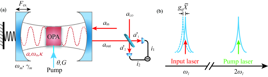
Figure 1: (Color online) (a) Schematics of the cavity optomechanical (COM) system consisting of a Fabry-Pérot cavity coupled to a degenerate optical parametric amplifier (OPA). One or even two mirror coatings are usually directly placed on the spherical and polished surfaces of the nonlinear crystal that generates the squeezed vacuum and produces parametric amplification Wu et al. (1986); Grangier et al. (1987). In this setup, an external weak force $F_{\mathrm{ex}}$ acting on the mechanical resonator can be measured with homodyne detection. (b) Frequency spectrum of the OPA-assisted COM system. An input laser drives the optical cavity at frequency $\omega_{l}$, thus, a pump laser beam with frequency $2\omega_{l}$ is applied to the degenerate OPA. The dashed curve shows the static frequency shift $g_{0}\bar{X}$ at the cavity resonance because of radiation pressure.

II Model and solution

Figure 1 shows the schematics of intracavity squeezing in an OPA-assisted Fabry-Pérot cavity Wu et al. (1986); Grangier et al. (1987). Previous researches on such squeezed quantum systems have usually focused on enhanced mechanical cooling Huang and Agarwal (2009a); Huang and Chen (2018); Lau and Clerk ; Asjad et al. or squeezing Lü et al. (2015); Agarwal and Huang (2016); Gu et al. (2018) and enhanced light-matter coupling Qin et al. (2018); Leroux et al. (2018); Huang and Agarwal (2009b). When light pressure couples to a movable mirror, coherent states are transformed into squeezed states of light Braginskiĭ and Manukin (1967), and this type of squeezing, referred to as ponderomotive squeezing Schnabel (2017), can be only used to evade back-action and thus it is less extensive than externally injecting a squeezed light Corbitt et al. (2006) or generating intracavity squeezing via an OPA Wu et al. (1986). We note that in a recent experiment, the OPA effect was improved by 14 orders of magnitude via symmetry breaking at a microcavity surface Zhang et al. (2018). Other approaches to generate intracavity squeezing include, e.g., Kerr media Collett and Gardiner (1984); Bondurant (1986); Yin et al. (2018) or dissipative COM devices Xuereb et al. (2011); Kronwald et al. (2014); Bai et al. (2019). We also note that by using mechanical squeezing Pirkkalainen et al. (2015); Ockeloen-Korppi et al. (2017); Burd et al. (2019); Qin et al. (2019), the sensitivity of detecting small displacements was improved by a factor of up to 7 Burd et al. (2019).

To realize weak-force sensing with OPA, we assume that only one optical mode is coupled to the mechanical mode. Thus, the Hamiltonian of the COM system can be described as Agarwal and Huang (2016):

$$H_{0} =\hbar\omega_{a}a^{\dagger}a+\frac{p^{2}}{2m}+\frac{1}{2}m\omega_{m}^{2}x^{2}+\hbar\frac{\omega_{a}}{L}xa^{\dagger}a$$

$$\quad\,+i\hbar G\left(e^{i\theta}a^{\dagger 2}e^{-2i\omega_{l}t}-e^{-i\theta}a^{2}e^{2i\omega_{l}t}\right),$$ (1)

where $\omega_{a}$ denotes the optical resonant frequency; $x$ and $p$ refer to the position and momentum operators of the vibrating mechanical oscillator having an effective mass $m$ and an angular frequency $\omega_{m}$, respectively. In addition, $a$ and $a^{\dagger}$ are the annihilation and creation operators of the cavity mode, respectively. We have furthermore used $G$ to denote the nonlinear gain of degenerate OPA with $\theta$ being the phase of the pump field driving the OPA medium. For the sake of simplicity, we define dimensionless position and momentum operators of the mechanical mode as $X=\left.x\middle/x_{\mathrm{zpf}}\right.$, $P=\left.p\middle/p_{\mathrm{zpf}}\right.$, where $x_{\mathrm{zpf}}$ and $p_{\mathrm{zpf}}$ are the standard deviations of the zero-point motion and momentum of the oscillator, respectively, $x_{\mathrm{zpf}}=\sqrt{\left.\hbar\middle/\left(m\omega_{m}\right)\right.}$, $p_{\mathrm{zpf}}=\sqrt{\hbar m\omega_{m}}$, and the operators $X$ and $P$ satisfy the commutation relation $\left[X,P\right]=i$. Thus, in a rotating frame, the Hamiltonian can be rewritten as follows:

$$H =\hbar\Delta_{a}a^{\dagger}a+\frac{\hbar}{2}\omega_{m}\left(X^{2}+P^{2}\right)+\hbar g_{0}a^{\dagger}aX$$

$$\quad\,+i\hbar G\left(e^{i\theta}a^{\dagger 2}-e^{-i\theta}a^{2}\right),$$ (2)

where $g_{0}=\left.x_{\mathrm{zpf}}\omega_{a}\middle/L\right.$ represents the single photon coupling strength of the COM interaction. The first and second terms in Eq. (2) denote the sum of the free energy of the cavity field and the mechanical mode without external forces, respectively. And the last two terms respectively describe the COM interaction and the contribution of an OPA. By introducing dissipation and noise terms, the Heisenberg-Langevin equations can be written as:

$$\dot{X} =\omega_{m}P,$$

$$\dot{P} =-\omega_{m}X-\gamma_{m}P-g_{0}a^{\dagger}a+\sqrt{2\gamma_{m}}\left(f_{\mathrm{th}}+f_{\mathrm{ex}}\right),$$

$$\dot{a} =-\left(i\Delta_{a}+\frac{\kappa}{2}\right)a-ig_{0}Xa+2Ge^{i\theta}a^{\dagger}+\sqrt{\kappa}a_{\mathrm{in}},$$ (3)

where $\Delta_{a}=\omega_{a}-\omega_{l}$ is the detuning of the input light frequency ($\omega_{a}$) with respect to the cavity resonant frequency ($\omega_{l}$); $a_{\mathrm{in}}$ characterizes the input field driving the cavity, which fulfils Wimmer et al. (2014); Huang and Chen (2018): $\left\langle a_{\mathrm{in}}\left(t\right)a^{\dagger}_{\mathrm{in}}\left(t^{\prime}\right)\right\rangle=\delta\left(t-t^{\prime}\right)$. Moreover, $f_{\mathrm{th}}=\left.\xi\middle/\sqrt{2\hbar m\gamma_{m}\omega_{m}}\right.$ and $f_{\mathrm{ex}}=\left.F_{\mathrm{ex}}\middle/\sqrt{2\hbar m\gamma_{m}\omega_{m}}\right.$ are the scaled thermal and external forces with zero mean values, respectively. The Brownian thermal noise operator $\xi$ obeys the correlation function Giovannetti and Vitali (2001):

$$\left\langle\xi\left(t\right)\xi\left(t^{\prime}\right)\right\rangle=m\hbar\gamma_{m}\int\frac{\mathrm{d}\omega}{2\pi}e^{-i\omega\left(t-t^{\prime}\right)}\omega\left[\coth{\frac{\hbar\omega}{2k_{B}T}}+1\right],$$ (4)

where $k_{B}$ is the Boltzmann constant and $T$ is the mirror temperature of the thermal bath. Additionally, if the mechanical quality factor is large, $Q=\left.\omega_{m}\middle/\gamma_{m}\right.\gg 1$, the Brownian noise $\xi\left(t\right)$ describes a Markovian process that is delta-correlated Giovannetti and Vitali (2001):

$$\tfrac{1}{2}\left\langle\xi\left(t\right)\xi\left(t^{\prime}\right)+\xi\left(t^{\prime}\right)\xi\left(t\right)\right\rangle\simeq m\hbar\omega_{m}\gamma_{m}\left(2\bar{n}+1\right)\delta\left(t-t^{\prime}\right),$$ (5)

where $\bar{n}=\left[\exp\left(\left.\hbar\omega_{m}\middle/k_{B}T\right.\right)-1\right]^{-1}$ is the mean thermal phonon number. Under the approximation of thermal equilibrium and taking the classical limit $\hbar\omega_{m}\ll k_{B}T$ Bowen and Milburn (2015), the scaled thermal force obeys $\left\langle f_{\mathrm{th}}\left(t\right)f_{\mathrm{th}}\left(t^{\prime}\right)\right\rangle=\left(\left.k_{B}T\middle/\hbar\omega_{m}\right.\right)\delta\left(t-t^{\prime}\right)$ Wimmer et al. (2014).

Linearization or even semiclassical approximation are standard effective descriptions applied in case of strong optical drives, which are valid in both theory Motazedifard et al. (2016); Huang and Agarwal (2017) and experiments Safavi-Naeini et al. (2013); Shomroni et al. (2019); Basiri-Esfahani et al. (2019). Indeed, a strong quantum-optical drive can usually be treated as a semiclassical parameter. Thus, an operator (a q-number) describing such a drive can be replaced by a c-number. For example, in standard description of homodyne detection, which can be applied for quantum state tomography, a weak quantum signal is driven (i.e., mixed on a beam splitter) by a strong-laser mode (i.e., a local oscillator), which is described by a classical parameter (see Appendix D). Therefore, in case where the input optical field is a semiclassical coherent laser field Basiri-Esfahani et al. (2019), i.e., in the strong driving regime $\left|\alpha\right|\gg 1$ Huang and Agarwal (2017) (see Appendix B), we can expand each operator as the sum of its steady-state value and a small fluctuation, i.e., $P=\bar{P}+\delta P$, $X=\bar{X}+\delta X$, $a=\alpha+\delta a$, and $a_{\mathrm{in}}=\alpha_{\mathrm{in}}+\delta a_{\mathrm{in}}$. Here we choose the input field as the zero-phase reference, i.e., $\alpha_{\mathrm{in}}=\left|\alpha_{\mathrm{in}}\right|=\sqrt{\left.P_{\mathrm{in}}\middle/\hbar\omega_{l}\right.}$ with $P_{\mathrm{in}}$ being the input laser power Bowen and Milburn (2015). By setting all the time derivatives to zero, the steady-state values of the dynamical variables can be obtained as $\bar{P}=0$, $\bar{X}=\left.-g_{0}\alpha^{*}\alpha\middle/\omega_{m}\right.$ and

$$\alpha=\frac{\sqrt{\kappa}\alpha_{\mathrm{in}}}{2\sigma_{+}}\left(\kappa-2i\Delta+4Ge^{i\theta}\right)=\left|\alpha\right|e^{i\phi},$$ (6)

where $\sigma_{\pm}=\left.\kappa^{2}\middle/4\right.\pm\Delta^{2}\mp 4G^{2}$ and $\Delta=\Delta_{a}+g_{0}\bar{X}$ denotes the effective cavity detuning. Therefore, the phase of the intracavity amplitude becomes:

$$\phi =\arctan\left(\frac{4G\sin\theta-2\Delta}{4G\cos\theta+\kappa}\right).$$ (7)

We define the standard quadratures of the cavity field as $x_{a}=\left.\left(a+a^{\dagger}\right)\middle/\sqrt{2}\right.$, $p_{a}=\left.\left(a-a^{\dagger}\right)\middle/\left(\sqrt{2}i\right)\right.$. These are the canonical (i.e., dimensionless) position ($x_{a}$) and momentum ($p_{a}$) operators, also referred to as the amplitude and phase quadratures, which are related to the electric and magnetic fields of an optical mode, respectively. For simplicity, we set the integral constants to zero and neglect the higher-order terms $\delta a^{\dagger}\delta a$ and $\delta X\delta a$, then the linearized equations can be written as (a similar matrix form is given in Ref. Agarwal and Huang (2016)):

$$\dot{\mathrm{v}}=\mathrm{C}\mathrm{v}+\mathrm{A}\mathrm{v}_{\mathrm{in}}.$$ (8)

The operator vectors are $\mathrm{v}=\begin{pmatrix}X,&P,&x_{a},&p_{a}\end{pmatrix}^{\mathrm{T}}$ and $\mathrm{v}_{\mathrm{in}}=\begin{pmatrix}0,&f_{\mathrm{in}},&x_{a}^{\mathrm{in}},&p_{a}^{\mathrm{in}}\end{pmatrix}^{\mathrm{T}}$, where $f_{\mathrm{in}}=f_{\mathrm{th}}+f_{\mathrm{ex}}$, and superscript $\mathrm{T}$ represents the transpose of a matrix. The quadratures of the input field ($x_{a}^{\mathrm{in}}$ and $p_{a}^{\mathrm{in}}$), are defined analogously to $x_{a}$ and $p_{a}$. The coefficient matrix $\mathrm{C}$ and the noise matrix $\mathrm{A}$ are given in Appendix B.

In standard homodyne detection, which enables quantum state tomography, a quantum optical field [in our case $a_{\mathrm{out}}\left(t\right)$] is mixed with a strong classical laser field $\alpha_{\mathrm{LO}}$ (i.e., a local oscillator, LO) at a balanced beam splitter. The homodyne signal (say, the photocurrent $i_{\mathrm{det}}$) corresponds to the difference of the photon numbers at the two output ports of the beam splitter. This signal is proportional to the generalized phase-dependent quadrature operator $x_{a,\mathrm{out}}^{\varphi}$, as follows Leonhardt (1997):

$$i_{\mathrm{det}} =\left|\alpha_{\mathrm{LO}}\right|\left(e^{i\varphi}a^{\dagger}_{\mathrm{out}}+e^{-i\varphi}a_{\mathrm{out}}\right)$$

$$=\sqrt{2}\left|\alpha_{\mathrm{LO}}\right|x_{a,\mathrm{out}}^{\varphi},$$ (9)

where $\varphi$ and $\alpha_{\mathrm{LO}}$ respectively correspond to the phase and amplitude of the local oscillator, which are arbitrary (see Appendix D for more details). Note that by changing the phase $\varphi$ of the local oscillator, a complete quantum state tomography can be implemented with this method Leonhardt (1997). As depicted in Figure 1, homodyne detection is a phase-referenced technique, where direct measurement of an optical field produces a stochastic photocurrent that is proportional to the rotated quadrature $x^{\varphi}_{\mathrm{a,out}}$ and the measured quadrature is dependent on the phase of the local oscillator $\alpha_{\mathrm{LO}}$. We also note that the quadratures for arbitrary phases of the local oscillator can be measured. Thus, homodyne tomography can be performed to reconstruct the output field with arbitrary phase Miranowicz et al. (2014). However, for brevity, we further study only the output canonical momentum quadrature, i.e., $\varphi=\left.\pi\middle/2\right.$. Hence, the external force can be expressed as:

$$F=\frac{1}{F_{f}\left(\omega\right)}x^{\left.\pi\middle/2\right.}_{\mathrm{a,out}}=\frac{1}{F_{f}\left(\omega\right)}\tilde{p}_{a}^{\mathrm{out}}=\tilde{f}_{\mathrm{ex}}+\tilde{f}_{\mathrm{add}}.$$ (10)

where $F_{f}\left(\omega\right)=gf_{-}\chi_{-}\chi_{m}\sqrt{2\kappa\gamma_{m}}$, and $g=\sqrt{2}g_{0}\left|\alpha\right|$ represents the effective linearized optomechanical coupling rate. Therefore, noise of the added force can be described by

$$f_{\mathrm{add}}\left(\omega\right)=\tilde{f}_{\mathrm{th}}+X_{a}\left(\omega\right)\tilde{x}_{a}^{\mathrm{in}}+P_{a}\left(\omega\right)\tilde{p}_{a}^{\mathrm{in}},$$ (11)

where $\tilde{f}_{r}\equiv f_{r}\left(\omega\right)$, $\tilde{s}_{a}^{u}\equiv s_{a}^{u}\left(\omega\right)$, for $s=x,\,p$, $u=\mathrm{in,\,out}$, and $r=\mathrm{in,\,th,\,ex,\,add}$. Moreover, the coefficients in Eq. (11) are given by:

$$X_{a}\left(\omega\right)=\left.\left(\mu_{+}\lambda_{+}\chi_{-}\kappa\right)\middle/F_{f}\right.,\quad P_{a}\left(\omega\right)=\left.\left(\chi_{-}\kappa-1\right)\middle/F_{f}\right..$$ (12)

The parameters $f_{\pm}$, $\chi_{\pm}$, $\mu_{\pm}$, and $\lambda_{\pm}$ are defined in Appendix C.

We use the symmetric part ($S_{\mathrm{FF}}$) of the added noise power spectral density ($S_{\mathrm{F}}$) to characterize the sensitivity of the force measurement, given by (see Appendix D for more details):

$$S_{\mathrm{FF}}\left(\omega\right) =\frac{S_{\mathrm{F}}\left(\omega\right)+S_{\mathrm{F}}\left(-\omega\right)}{2}$$

$$=\underbrace{\frac{k_{B}T}{\hbar\omega_{m}}}_{\text{thermal noise}}+\underbrace{\frac{1}{2}\left|X_{a}\left(\omega\right)\right|^{2}}_{\text{backaction noise}}+\underbrace{\frac{1}{2}\left|P_{a}\left(\omega\right)\right|^{2}}_{\text{shot noise}},$$ (13)

where we have used the correlation functions and the bath cross-correlated terms of the measured symmetrized power spectral density are cancelled out. The first term of $S_{\mathrm{FF}}\left(\omega\right)$ represents the thermal Brownian noise. The second term is the back-action noise, which is proportional to the input power $P_{\mathrm{in}}$ and the square of the coupling strength $g^{2}$. Very recently, Corbitt et al. have presented a testbed for the broadband measurement of quantum back action at room temperature Cripe et al. (2019). The third term denotes the shot noise that is inversely proportional to the input power $P_{\mathrm{in}}$. Since beating the SQL in an optomechanical sensor by cavity detuning has been studied in Ref. Arcizet et al. (2006) and the highest parametric gain is achieved at the cavity resonance Schnabel (2017), in the following, we neglect thermal noise and other technical noises and restrict our discussion to the case of $\Delta=0$. We note that the idea of utilizing a nondegenerate OPA-assisted COM to circumvent measured backaction and surpass the SQL has been proposed in Ref. Wimmer et al. (2014). This scheme is based on an antinoise process (using an oscillator with an effective negative mass) via destructive quantum interference, i.e., the so-called coherent quantum noise cancellation (CQNC) Tsang and Caves (2010, 2012); Gebremariam et al. (2020). Additionally, a quantum-mechanics-free subsystem (QMFS) Tsang and Caves (2012), proposed by Tsang and Caves Tsang and Caves (2010), was first realized in Ref. Ockeloen-Korppi et al. (2016).

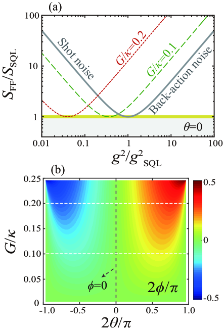
Figure 2: (Color online) (a) Noise power spectral density $\left.S_{\mathrm{FF}}\middle/S_{\mathrm{SQL}}\right.$ is plotted as a function of the scaled square of the coupling strength $\left.g^{2}\middle/g^{2}_{\mathrm{SQL}}\right.$ and of the OPA parametric gain $G$. The gray solid line corresponds to the non-OPA case. (b) Phase $\phi$, given in Eq. (7), of the intracavity field versus the OPA parameters: the phase $\theta$ and gain $G$ in the units of the damping rate $\kappa$. Here we assume the resonance condition $\Delta=0$.

In order to compare force sensing in the presence and in the absence of OPA, we first concern about force sensing of a standard COM system at a resonant frequency. For such a scheme, the sensitivity cannot surpass the SQL without an OPA [see Figure 2(a)]. Moreover, if we assume the linewidth of the cavity to be much larger than any measurement frequency of interest, $\kappa\gg\omega$, the symmetrized noise spectral density can be simplified as follows Motazedifard et al. (2016); Wimmer et al. (2014):

$$S_{\mathrm{FF}}^{\mathrm{st}}=\frac{g^{2}}{\kappa\gamma_{m}}+\frac{1}{16}\frac{\kappa}{g^{2}\gamma_{m}}\frac{1}{\left|\chi_{m}\right|^{2}},$$ (14)

where the susceptibility of the mechanical oscillator ($\chi_{m}$) has been defined in Appendix B. Thus, we obtain $S_{\mathrm{FF}}^{\mathrm{st}}\geq\left(2\gamma_{m}\left|\chi_{m}\right|\right)^{-1}=S_{\mathrm{SQL}}$, $g_{\mathrm{SQL}}^{2}=\left.\kappa\middle/\left(4\left|\chi_{m}\right|\right)\right.$.

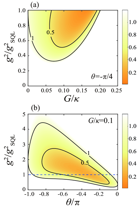
Figure 3: (Color online) Noise power spectral density $\left.S_{\mathrm{FF}}\middle/S_{\mathrm{SQL}}\right.$ as the functions of the scaled square of the coupling strength, $\left.g^{2}\middle/g^{2}_{\mathrm{SQL}}\right.$, and the parametric gain $G$ or the parametric phase $\theta$. The other parameters are set as (a) $\theta=\left.-\pi\middle/4\right.$ and (b) $\left.G\middle/\kappa\right.=0.1$.

Subsequently, we study the case of the zero pump phase ($\theta=0$) of the COM system with an OPA. In this case, the symmetrized noise power spectral density $S_{\mathrm{FF}}$ can be reduced to:

$$S_{\mathrm{FF}}\left(\theta=0\right)=\frac{g^{2}\kappa}{4\gamma_{m}\left(\left.\kappa\middle/2\right.-2G\right)^{2}}+\frac{\left(\left.\kappa\middle/2\right.-2G\right)^{2}}{4\kappa\gamma_{m}g^{2}\left|\chi_{m}\right|^{2}}.$$ (15)

Therefore, we also have $S_{\mathrm{FF}}\left(\theta=0\right)\geq\left.1\middle/\left(2\gamma_{m}\left|\chi_{m}\right|\right)\right.=S_{\mathrm{SQL}}$, indicating that the detection sensitivity still cannot surpass the SQL when $\theta=0$. As Figure 2(a) shows, in the absence of OPA ($\left.G\middle/\kappa\right.=0$), the minimum of $\left.S_{\mathrm{FF}}\middle/S_{\mathrm{SQL}}\right.$ equals to 1 when the coupling strength is $g=g_{\mathrm{SQL}}$. The optimal COM parameter $g_{\mathrm{opt}}$ can be obtained by solving $\left|X_{a}\right|=\left|P_{a}\right|$, which gives $g_{\mathrm{opt}}^{\left(\theta=0\right)}=\left.\left|\kappa-4G\right|\middle/\left(2\sqrt{\kappa\left|\chi_{m}\right|}\right)\right.$. Furthermore, by the inspection of Eq. (7) under the resonance condition $\Delta=0$, it is easy to understand why the intracavity field phases $\phi$ for $\pm\theta$, corresponding to symmetric points on both sides of the dividing dashed line in Figure 2(b), have opposite signs. By comparing the phases $\phi$ for $\theta=\pm\pi/2$ and $G/\kappa=1/4$, corresponding to the darkest blue and darkest red points in Figure 2(b), we find that the intracavity field phases $\phi$ are $\pi/2$-shifted for the opposite phases $\theta$ of the OPA pump for these special values of $G=\kappa/4$ and $\Delta=0$. This conclusion can easily be drawn by analyzing Eq. (7) for the discussed parameters.

From the analyses made above, we have identified that it is impossible for weak-force sensing to exceed the SQL with non-OPA or $\theta=0$. As depicted in Figure 2(a), owing to the reduction of shot noise, $S_{\mathrm{FF}}$ first decreases with the COM coupling strength increasing until the turning point (corresponding to $S_{\mathrm{FF}}=S_{\mathrm{SQL}}$); then, the backaction noise is dominant, leading $S_{\mathrm{FF}}$ to increase. Hence, the SQL can be reached at the minimum point $g=g_{\mathrm{opt}}$ and the optimum coupling strength can be lowered by adjusting the OPA pump gain $G$. In calculations, we use experimentally accessible parameters Bowen and Milburn (2015), i.e., $\left.\omega_{l}\middle/2\pi\right.=2\times 10^{14}\,\mathrm{Hz}$, $\left.\gamma_{m}\middle/2\pi\right.=1\,\mathrm{kHz}$, $\left.\omega_{m}\middle/2\pi\right.=10\,\mathrm{MHz}$, $\left.\kappa\middle/2\pi\right.=10\,\mathrm{MHz}$, $\left.g_{0}\middle/2\pi\right.=100\,\mathrm{Hz}$ and $P_{\mathrm{in}}=700\,\mathrm{nW}$.

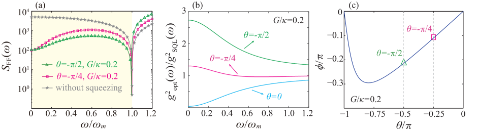
Figure 4: (Color online) (a) Noise power spectral density $S_{\mathrm{FF}}(\omega)$ at the optimal power vs frequency $\omega$. The gray curve corresponds to $S_{\mathrm{SQL}}(\omega)$ without squeezing. (b) Optimal coupling strength as functions of the OPA pump phase and the detection frequency. (c) Intracavity phase with varying the OPA pump phase. The parametric gain is set as $\left.G\middle/\kappa\right.=0.2$.

To overcome the SQL, we study the impact of the OPA pump phase on weak-force sensing. Figure 3 shows the sensitivity as the functions of $\left.g^{2}\middle/g^{2}_{\mathrm{SQL}}\right.$ and the parametric gain $G$ in the low-frequency domain. Specifically, as depicted in Figure 3(a), the sensitivity can be improved more than twice with an OPA when choosing appropriate parameters and the coupling strength required to increase the sensitivity becomes much smaller than $g_{\mathrm{SQL}}$. Additionally, according to Eqs. (12) and (13), we are likely to enhance the detection sensitivity by tuning $\sin\theta$ to satisfy $2G\sin\theta+g^{2}\chi_{m}\cos^{2}\phi\approx 0$, for suppressing the back-action noise to the limit. Furthermore, we utilize $\sin\theta<0$ in Figure 3(b) to reduce quantum noise and improve the measurement accuracy. We note that very recently, optimal cavity squeezing up to $30\,\mathrm{dB}$ has been predicted theoretically Macrí et al. , and single label-free sensing of nanoparticles has been studied with a spinning resonator Jing et al. (2018) and exposed-core fiber Mauranyapin et al. (2019). In particular, Miao et al. have recently proposed a new fundamental limit to the precision of a gravitational-wave detector Miao et al. (2019), which provides an answer of how far we can push the detector sensitivity.

In Figure 4, we consider the variation of the optimal symmetrized noise spectral density $S_{\mathrm{FF}}(\omega)$ with the increase of the frequency $\omega$, analogously similar to the corresponding illustration in Ref. Wimmer et al. (2014). Here we set the OPA pump gain as $\left.G\middle/\kappa\right.=0.2$. As illustrated in Figure 4(a), the SQL can be well suppressed at frequencies below the mechanical resonance, i.e., we can increase the force sensitivity by nearly two-orders of magnitude in the low-frequency domain. Note that recently, a quantum expander for gravitational-wave observatories has been demonstrated in Ref. Korobko et al. , where quantum uncertainty can be squeezed even at high frequencies, while maintaining the low-frequency sensitivity unchanged, thus, expanding the detection bandwidth. In Figures 4(b)-4(c), we depict the two key parameters, i.e., the optomechanical coupling strength $g_{\mathrm{opt}}$ and intracavity phase $\phi$, required for the minimum symmetrized noise spectral density, in the limits of different phases $\theta$ and frequencies $\omega$.

From what has been discussed above, it would be reasonable to overcome the SQL by tuning the OPA pump phase. However, because of this nonzero pump phase, the canonical position ($x_{a}$) and momentum ($p_{a}$) operators become correlated, causing a loss of quantum efficiency which cannot be ignored (see Appendix B for more details). For instance, the dashed line in Figure 2(b) illustrates the case of $\theta=\phi=0$, in which $x_{a}$ and $p_{a}$ are decoupled, circumventing quantum efficiency losses successfully, but a loss of mechanical-mode information is inevitable in the regions divided by the dashed line. Additionally, as the frequency increases, there is an unavoidable quantum efficiency loss shown in Figure 4. Nonetheless, in the specific regime where $\kappa\gg\omega$ and $\Delta=0$, we are able to achieve quantum noise reduction without losing mechanical-mode information. In the limit of $\kappa\gg\omega$, according to the coefficients given in Appendix C, we find:

$$\mu_{\pm}\lambda_{\pm}\approx\frac{4G\sin\theta\pm 2g^{2}\chi_{m}\sin^{2}\left(\phi+\phi_{\pm}\right)}{\kappa\mp 4G\cos\theta\pm g^{2}\chi_{m}\sin\left(2\phi\right)},$$ (16)

where $\phi_{\pm}=\left(1\pm 1\right)\left.\pi\middle/4\right.$. Hence, we obtain $\tan\phi=\mu_{-}\lambda_{-}$ and $\cot\phi\neq\mu_{+}\lambda_{+}$, i.e., $f_{+}=0$ and $f_{-}\neq 0$. Utilizing the input-output relations, the output canonical position quadrature $x_{a}^{\mathrm{out}}$ does not contain $f_{\mathrm{in}}$; thus, the detected squeezed quadrature carries all of the mechanical quantum information, and the SQL can be reached or surpassed, as shown in Figures 2-3, whose parameters utilized in calculations obey the approximation $\kappa\gg\omega$.

III Conclusion

In conclusion, we have investigated weak-force sensing in a squeezed cavity and theoretically showed that (i) the SQL cannot be surpassed in the case of $G=0$ or $\theta=0$, (ii) the measurement precision of weak-force detection can be remarkably improved at the coupling strength smaller than $g_{\mathrm{SQL}}$ by tuning the parametric phase and gain, and (iii) under the approximation of $\kappa\gg\omega$, quantum noise can be reduced without losing mechanical-mode information. Our work provides new insight in strengthening the sensitivity of a force sensor with the assistance of intracavity squeezing, which can be also extended into other systems of quantum sensing with e.g., waveguide Allen et al. ; Mauranyapin et al. (2019), interferometer Ouyang et al. (2019), or parity-time ($\mathcal{PT}$) symmetric microcavity Liu et al. (2016); Özdemir et al. (2019); Zhong et al. (2019). In the future, we plan to extend our work to study the weak-force measurement with the help of two-mode squeezing or quantum entanglement Palomaki et al. (2013); Takeuchi et al. (2019); Barzanjeh et al. (2019), squeezed mechanical modes Suh et al. (2014); Burd et al. (2019), or squeezed sources in hybrid COM devices Li et al. (2019c); Xu et al. (2019).

APPENDIX A DERIVATION OF THE EFFECTIVE HAMILTONIAN

In our system, the cavity with resonant frequency $\omega_{a}$ and damping rate $\kappa$, is driven by an input beam $a_{\mathrm{in}}$ at frequency $\omega_{l}$. The left mirror is movable, which supports a mechanical mode with frequency $\omega_{m}$ and damping rate $\gamma_{m}$. An external force $F_{\mathrm{ex}}$ is applied on the left-hand mirror and the cavity adjoins the movable mirror with coupling strength $g_{0}=\left.x_{\mathrm{zpf}}\omega_{a}\middle/L\right.$, where $L$ is the length of the cavity. When a pump field at frequency $2\omega_{l}$ interacts with a second-order nonlinear optical crystal, the output frequency becomes $\omega_{l}$ Huang and Agarwal (2017). The nonlinear gain $G$ of the degenerate OPA with pump phase $\theta$ is proportional to the pump field. By transforming into a frame rotating at the incoming laser frequency $\omega_{l}$ with $\Delta_{a}=\omega_{a}-\omega_{l}$, Hamiltonian (1) can be rewritten as:

$$H=-i\hbar U\frac{\mathrm{d}U^{\dagger}}{\mathrm{d}t}+UH_{0}U^{\dagger},$$ (A1)

via the unitary transformation $U\left(t\right)=\exp\left(i\omega_{l}a^{\dagger}at\right)$. Using the relation

$$e^{A}Be^{-A}=B+\left[A,B\right]+\frac{1}{2!}\left[A,\left[A,B\right]\right]+\cdots,$$ (A2)

we obtain Huang and Agarwal (2009a, b):

$$H =\hbar\Delta_{a}a^{\dagger}a+\hbar\frac{\omega_{a}}{L}xa^{\dagger}a+\frac{p^{2}}{2m}+\frac{1}{2}m\omega_{m}^{2}x^{2}$$

$$\quad\,+i\hbar G\left(e^{i\theta}a^{\dagger 2}-e^{-i\theta}a^{2}\right),$$ (A3)

where $m$ stands for the effective mass of the mechanical mode, while $x$ and $p$ represent the position and momentum operators, respectively.

In the Heisenberg picture, the dynamics of an operator $\mathcal{O}$ of a quantum system can be determined via the Heisenberg equation of motion:

$$\dot{\mathcal{O}}\left(t\right)=\frac{1}{i\hbar}\left[\mathcal{O}\left(t\right),H\left(t\right)\right].$$ (A4)

By introducing dissipation and noise terms, we have:

$$\dot{X} =\omega_{m}P,$$

$$\dot{P} =-\omega_{m}X-\gamma_{m}P-g_{0}a^{\dagger}a+\sqrt{2\gamma_{m}}\left(f_{\mathrm{th}}+f_{\mathrm{ex}}\right),$$

$$\dot{a} =-i\left(\Delta_{a}+g_{0}X\right)a+2Ge^{i\theta}a^{\dagger}-\frac{\kappa}{2}a+\sqrt{\kappa}a_{\mathrm{in}},$$ (A5)

where $\kappa$ and $\gamma_{m}$ are the decay rates of the optical cavity and the mechanical oscillator, respectively. $X=\left.x\middle/x_{\mathrm{zpf}}\right.$ and $P=\left.p\middle/p_{\mathrm{zpf}}\right.$ denote the dimensionless displacement and momentum operators of the mechanical mode, where $x_{\mathrm{zpf}}=\sqrt{\left.\hbar\middle/\left(m\omega_{m}\right)\right.}$ and $p_{\mathrm{zpf}}=\sqrt{\hbar m\omega_{m}}$ are the zero-point position and momentum fluctuations, respectively. The input noise operator $a_{\mathrm{in}}\left(t\right)$ fulfills the correlation relations Wimmer et al. (2014); Huang and Chen (2018):

$$\left\langle a_{\mathrm{in}}^{\dagger}\left(t\right)a_{\mathrm{in}}\left(t^{\prime}\right)\right\rangle =0,$$

$$\left\langle a_{\mathrm{in}}\left(t\right)a_{\mathrm{in}}^{\dagger}\left(t^{\prime}\right)\right\rangle =\delta\left(t-t^{\prime}\right),$$

$$\left\langle a_{\mathrm{in}}\left(t\right)a_{\mathrm{in}}\left(t^{\prime}\right)\right\rangle =\left\langle a_{\mathrm{in}}^{\dagger}\left(t\right)a_{\mathrm{in}}^{\dagger}\left(t^{\prime}\right)\right\rangle=0.$$ (A6)

Moreover, $f_{\mathrm{th}}$ and $f_{\mathrm{ex}}$ represent the scaled thermal and external forces given, respectively, by:

$$f_{\mathrm{th}}=\frac{\xi}{\sqrt{2\hbar m\gamma_{m}\omega_{m}}},\quad f_{\mathrm{ex}}=\frac{F_{\mathrm{ex}}}{\sqrt{2\hbar m\gamma_{m}\omega_{m}}},$$ (A7)

where $\xi$ and $F_{\mathrm{ex}}$ are the corresponding thermal and external forces, respectively.

When the mechanical resonator is in thermal equilibrium at environment temperature $T$, the Bose-Einstein statistics determines the occupancy probability $p\left(n\right)$ of each energy level, given by:

$$p\left(n\right)=\delta^{n}\left(1-\delta\right),$$ (A8)

where $\delta=\exp\left[\left.-\hbar\omega_{m}\middle/\left(k_{B}T\right)\right.\right]$. Therefore, the mean number $\bar{n}$ of phonons in thermal equilibrium is

$$\bar{n}=\sum_{n=0}^{\infty}np\left(n\right)=\left(\delta^{-1}-1\right)^{-1}.$$ (A9)

In the high temperature limit of $k_{B}T\gg\hbar\omega_{m}$, Eq. (A9) can be simplified to the familiar expression:

$$\bar{n}\approx\frac{k_{B}T}{\hbar\omega_{m}},$$ (A10)

and according to Eq. (5), the thermal noise force satisfies the correlation function as follows Wimmer et al. (2014):

$$\left\langle\xi\left(t\right)\xi\left(t^{\prime}\right)\right\rangle=2m\gamma_{m}k_{B}T\delta\left(t-t^{\prime}\right).$$ (A11)

Combining Eq. (A7) with Eq. (A11), we obtain:

$$\left\langle f_{\mathrm{th}}\left(t\right)f_{\mathrm{th}}\left(t^{\prime}\right)\right\rangle=\frac{k_{B}T}{\hbar\omega_{m}}\delta\left(t-t^{\prime}\right).$$ (A12)

Hence, Eq. (A12) becomes Wimmer et al. (2014):

$$\left\langle f_{\mathrm{th}}\left(t\right)f_{\mathrm{th}}\left(t^{\prime}\right)\right\rangle=\bar{n}\delta\left(t-t^{\prime}\right).$$ (A13)

APPENDIX B LINEAR RESPONSE

To solve the nonlinear Heisenberg-Langevin equations in Eq. (3), we linearize the operators around the steady-state values $\left(\bar{X},\,\bar{P},\,\alpha,\,\bar{f}_{\mathrm{th}},\,\bar{f}_{\mathrm{ex}},\,\alpha_{\mathrm{in}}\right)$, i.e., insert the ansatz

$$X =\bar{X}+\delta X, P =\bar{P}+\delta P,$$

$$a =\alpha+\delta a, f_{\mathrm{th}} =\bar{f}_{\mathrm{th}}+\delta f_{\mathrm{th}},$$

$$f_{\mathrm{ex}} =\bar{f}_{\mathrm{ex}}+\delta f_{\mathrm{ex}}, a_{\mathrm{in}} =\alpha_{\mathrm{in}}+\delta a_{\mathrm{in}},$$ (B1)

into Eq. (A5), and retain only the first-order terms, then we obtain:

$$\dot{X} =\omega_{m}P,$$

$$\dot{P} =-\omega_{m}X-\gamma_{m}P-g_{0}\left(\alpha^{*}a+\alpha a^{\dagger}\right)+\sqrt{2\gamma_{m}}f_{\mathrm{in}},$$

$$\dot{a} =-\left(i\Delta_{a}+\frac{\kappa}{2}\right)a-ig_{0}\left(\bar{X}a+\alpha X\right)+2Ge^{i\theta}a^{\dagger}+\sqrt{\kappa}a_{\mathrm{in}}.$$ (B2)

where $f_{\mathrm{in}}=f_{\mathrm{th}}+f_{\mathrm{ex}}$ and we consider the thermal and external noises average to $0$. For simplicity, we set the integral constants to zero.

When all time derivatives vanish, the steady-state values fulfill the self consistent equations:

$$0 =\omega_{m}\bar{P},$$

$$0 =-\omega_{m}\bar{X}-\gamma_{m}\bar{P}-g_{0}\alpha^{*}\alpha,$$

$$0 =-\left(i\Delta_{a}+\frac{\kappa}{2}\right)\alpha-ig_{0}\bar{X}\alpha+2Ge^{i\theta}\alpha^{*}+\sqrt{\kappa}\alpha_{\mathrm{in}}.$$ (B3)

The steady-state solution of Eq. (B) can be given by: $\bar{P}=0$, $\bar{X}=\left.-g_{0}n_{a}\middle/\omega_{m}\right.$, and

$$\alpha=\frac{\sqrt{\kappa}}{2\sigma_{+}}\left[\left(\kappa-2i\Delta\right)\alpha_{\mathrm{in}}+4Ge^{i\theta}\alpha_{\mathrm{in}}^{*}\right]=\left|\alpha\right|e^{i\phi},$$ (B4)

where $\sigma_{\pm}=\left.\kappa^{2}\middle/4\right.\pm\Delta^{2}\mp 4G^{2}$ and $\phi$ is the phase of the intracavity field. We have defined the effective detuning ($\Delta=\Delta_{a}+g_{0}\bar{X}$) and the mean intracavity photon number ($n_{a}=\left|\alpha\right|^{2}$).

Since phase is relative while phase difference is absolute, we focus on the phase difference between the external and internal optical fields and choose the incoming field as the zero phase reference, i.e., $\alpha_{\mathrm{in}}=\left|\alpha_{\mathrm{in}}\right|=\sqrt{\left.P_{\mathrm{in}}\middle/\hbar\omega_{l}\right.}$, where $P_{\mathrm{in}}$ denotes the input laser power Bowen and Milburn (2015). Thus, Eq. (B4) can be simplified to the following expression:

$$\alpha=\frac{\sqrt{\kappa}\alpha_{\mathrm{in}}}{2\sigma_{+}}\left(\kappa-2i\Delta+4Ge^{i\theta}\right)=\left|\alpha\right|e^{i\phi}.$$ (B5)

The assumption that $\alpha_{\mathrm{in}}$ is real, makes the phase $\phi$ dependent on $\kappa$, $G$, $\Delta$, and $\theta$, as follows:

$$\phi=\arctan\left(\frac{4G\sin\theta-2\Delta}{4G\cos\theta+\kappa}\right).$$ (B6)

Furthermore, $\left|\alpha\right|$ can be solved from Eq. (B5):

$$\left|\alpha\right|=\left|\frac{\sqrt{\kappa}\alpha_{\mathrm{in}}}{\sigma_{+}}\right|\sqrt{\sigma+2G\left(\kappa\cos\theta-2\Delta\sin\theta\right)},$$ (B7)

where $\sigma=\left.\kappa^{2}\middle/4\right.+\Delta^{2}+4G^{2}$. In the limit of $\Delta=0$, we use experimentally accessible parameters, which have been listed in Section II, to estimate the magnitude of $\left|\alpha\right|$:

$$\left|\alpha\right|\geq\left|\frac{2\sqrt{\kappa}\alpha_{\mathrm{in}}}{\kappa+4G}\right|\sim 10^{2}\gg 1.$$ (B8)

Hence, our calculations satisfy the strong-driving condition $\left|\alpha\right|\gg 1$ Huang and Agarwal (2017) and this linearized model has been proved valid and physically reasonable for our COM system.

To obtain the solutions of Eq. (B), we define the quadratures of input/output fields as $x_{a}^{u}=\left.\left(a_{u}+a^{\dagger}_{u}\right)\middle/\sqrt{2}\right.$ and $p_{a}^{u}=\left.\left(a_{u}-a^{\dagger}_{u}\right)\middle/\left(\sqrt{2}i\right)\right.$, where $u=\mathrm{in,\,out}$, analogously similar to the canonical position and momentum operators (given in Section II). Then, we have the linearized Heisenberg-Langevin equations given in Eq. (8), with the coefficients:

$$\mathrm{A} =\begin{pmatrix}0&0&0&0\\ 0&\sqrt{2\gamma_{m}}&0&0\\ 0&0&\sqrt{\kappa}&0\\ 0&0&0&\sqrt{\kappa}\\ \end{pmatrix},$$

$$\mathrm{C} =\begin{pmatrix}0&\omega_{m}&0&0\\ -\omega_{m}&-\gamma_{m}&-g\cos\phi&-g\sin\phi\\ g\sin\phi&0&C_{-}&S_{+}\\ -g\cos\phi&0&S_{-}&-C_{+}\\ \end{pmatrix},$$ (B9)

where $C_{\pm}=2G\cos\theta\pm\left.\kappa\middle/2\right.$, $S_{\pm}=2G\sin\theta\pm\Delta$, and $g=\sqrt{2}g_{0}\left|\alpha\right|$ is the effective linearized optomechanical coupling strength. Using the Fourier transform of Eq. (8), we obtain the linearized Heisenberg-Langevin equations in the frequency domain:

$$-i\omega\tilde{\mathrm{v}}=\mathrm{C}\tilde{\mathrm{v}}+\mathrm{A}\tilde{\mathrm{v}}_{\mathrm{in}},$$ (B10)

where $\tilde{\mathrm{v}}\equiv\mathrm{v}\left(\omega\right)=\begin{pmatrix}\tilde{X},&\tilde{P},&\tilde{x}_{a},&\tilde{p}_{a}\end{pmatrix}^{\mathrm{T}}$, $\tilde{\mathrm{v}}_{\mathrm{in}}\equiv\mathrm{v}_{\mathrm{in}}\left(\omega\right)=\begin{pmatrix}0,&\tilde{f}_{\mathrm{in}},&\tilde{x}_{a}^{\mathrm{in}},&\tilde{p}_{a}^{\mathrm{in}}\end{pmatrix}^{\mathrm{T}}$, and $\tilde{f}_{\mathrm{in}}\equiv\tilde{f}_{\mathrm{in}}\left(\omega\right)$; $\tilde{o}\equiv o\left(\omega\right)$, $\tilde{s}_{a}\equiv s_{a}\left(\omega\right)$, and $\tilde{s}_{a}^{\mathrm{in}}\equiv s_{a}^{\mathrm{in}}\left(\omega\right)$, for $o=X,\,P$, and $s=x,\,p$. From Eqs. (8) and (B), we can see when inserting a degenerate OPA medium into the Fabry-Pérot cavity, the canonical position ($x_{a}$) and momentum ($p_{a}$) operators are decoupled only if $S_{\pm}=0$. Specifically, in the dashed line showed in Fig. 2(b), substituting $\Delta=\theta=0$ ($S_{\pm}=0$) into Eq. (B10), we find that all the information is imprinted on the squeezed canonical momentum quadrature: $\tilde{x}_{a}=\rho_{-}\sqrt{\kappa}\tilde{x}_{a}^{\mathrm{in}}$, and

$$\tilde{p}_{a} =g^{2}\chi_{m}\rho_{+}\rho_{-}\sqrt{\kappa}\tilde{x}_{a}^{\mathrm{in}}+\rho_{+}\sqrt{\kappa}p_{a}^{\mathrm{in}}$$

$$\quad\,-g\chi_{m}\rho_{+}\sqrt{2\gamma_{m}}\tilde{f}_{\mathrm{in}},$$ (B11)

where $\rho_{\pm}=\left(\chi^{-1}\pm 2G\right)^{-1}$, and the susceptibilities of the cavity field and the mechanical oscillator are respectively defined as Huang and Chen (2018):

$$\chi\left(\omega\right) =\left(\left.\kappa\middle/2\right.-i\omega\right)^{-1},$$

$$\chi_{m}\left(\omega\right) =\omega_{m}\left(\omega_{m}^{2}-\omega^{2}-i\omega\gamma_{m}\right)^{-1}.$$ (B12)

Clearly, there are no correlations between this squeezed quadrature and its canonically conjugated quadrature $\tilde{x}_{a}$. However, on the both sides of the dividing line in Fig. 2(b), loss of mechanical-mode information inevitably exists, for the two quadratures are correlated. Therefore, we can conclude that under the resonance condition $\Delta=0$, quantum efficiency losses are dependent on the coupling of the quadratures $x_{a}$ and $p_{a}$ (i.e., the coefficients $S_{\pm}$ or the phase $\theta$ of the OPA pump). Our analysis of the stability conditions for the matrix $\mathrm{C}$, in Eq. (B), and the input-output relations are given in Appendix C.

APPENDIX C STABILITY CONDITIONS AND INPUT-OUTPUT RELATIONS

The system is stable only if all the eigenvalues $\lambda$ of the matrix $\mathrm{C}$ have negative real parts Jeffrey and Zwillinger (2000). It is well known that the characteristic equation $\left|\mathrm{C}-\lambda\mathrm{I}\right|=0$ can be reduced to:

$$\lambda^{4}+\mathrm{C}_{3}\lambda^{3}+\mathrm{C}_{2}\lambda^{2}+\mathrm{C}_{1}\lambda+\mathrm{C}_{0}=0.$$ (C1)

Hence, we obtain the stability conditions of the system from the Routh-Hurwitz criterion Jeffrey and Zwillinger (2000):

$$0 <\mathrm{C}_{3},$$

$$0 <\mathrm{C}_{3}\mathrm{C}_{2}-\mathrm{C}_{1},$$

$$0 <\mathrm{C}_{3}\mathrm{C}_{2}\mathrm{C}_{1}-\left(\mathrm{C}_{1}^{2}+\mathrm{C}_{3}^{2}\mathrm{C}_{0}\right).$$ (C2)

Specifically, all the external parameters should be chosen to satisfy the stability conditions in Eq. (C2), where the coefficients of the characteristic equation can be given by:

$$\mathrm{C}_{3} =\kappa+\gamma_{m},$$

$$\mathrm{C}_{2} =\omega_{m}^{2}+\kappa\gamma_{m}+\sigma_{+},$$

$$\mathrm{C}_{1} =\kappa\omega_{m}^{2}+\sigma_{+}\gamma_{m},$$

$$\mathrm{C}_{0} =\sigma_{+}\omega_{m}^{2}+2g^{2}G\omega_{m}\sin\left(2\phi-\theta\right)-g^{2}\omega_{m}\Delta.$$ (C3)

By solving Eq. (B10), we obtain the quadratures $\tilde{x}_{a}$ and $\tilde{p}_{a}$:

$$\tilde{x}_{a} =gf_{+}\chi_{+}\chi_{m}\sqrt{2\gamma_{m}}\tilde{f}_{\mathrm{in}}+\chi_{+}\sqrt{\kappa}\tilde{x}_{a}^{\mathrm{in}}$$

$$\quad\,+\mu_{-}\lambda_{-}\chi_{+}\sqrt{\kappa}\tilde{p}_{a}^{\mathrm{in}},$$

$$\tilde{p}_{a} =gf_{-}\chi_{-}\chi_{m}\sqrt{2\gamma_{m}}\tilde{f}_{\mathrm{in}}+\chi_{-}\sqrt{\kappa}\tilde{p}_{a}^{\mathrm{in}}$$

$$\quad\,+\mu_{+}\lambda_{+}\chi_{-}\sqrt{\kappa}\tilde{x}_{a}^{\mathrm{in}},$$ (C4)

where $\tilde{f}_{r}\equiv f_{r}\left(\omega\right)$, $\tilde{s}_{a}^{u}\equiv s_{a}^{u}\left(\omega\right)$, for $s=x,\,p$, $u=\mathrm{in,\,out}$, and $r=\mathrm{in,\,th,\,ex,\,add}$. Moreover, the coefficients in Eq. (C) are given by:

$$f_{-}\left(\omega\right) =\mu_{+}\lambda_{+}\sin\phi-\cos\phi,$$

$$f_{+}\left(\omega\right) =\sin\phi-\mu_{-}\lambda_{-}\cos\phi,$$

$$\chi_{\pm}\left(\omega\right) =\left(\lambda_{\pm}^{-1}-\mu_{+}\mu_{-}\lambda_{\mp}\right)^{-1},$$

$$\mu_{\pm}\left(\omega\right) =\mp\Delta+2G\sin\theta\pm g^{2}\chi_{m}\cos^{2}\phi,$$

$$\lambda_{\pm}\left(\omega\right) =\left[\chi^{-1}\mp 2G\cos\theta\pm\tfrac{1}{2}g^{2}\chi_{m}\sin\left(2\phi\right)\right]^{-1}.$$ (C5)

Using the input-output relations $\tilde{x}_{a}^{\mathrm{out}}=\sqrt{\kappa}\tilde{x}_{a}-\tilde{x}_{a}^{\mathrm{in}}$, $\tilde{p}_{a}^{\mathrm{out}}=\sqrt{\kappa}\tilde{p}_{a}-\tilde{p}_{a}^{\mathrm{in}}$, the quadratures of the output fields are given by:

$$\tilde{x}_{a}^{\mathrm{out}} =gf_{+}\chi_{+}\chi_{m}\sqrt{2\kappa\gamma_{m}}\tilde{f}_{\mathrm{in}}+\mu_{-}\lambda_{-}\chi_{+}\kappa\tilde{p}_{a}^{\mathrm{in}}$$

$$\quad\,+\left(\chi_{+}\kappa-1\right)\tilde{x}_{a}^{\mathrm{in}},$$

$$\tilde{p}_{a}^{\mathrm{out}} =gf_{-}\chi_{-}\chi_{m}\sqrt{2\kappa\gamma_{m}}\tilde{f}_{\mathrm{in}}+\mu_{+}\lambda_{+}\chi_{-}\kappa\tilde{x}_{a}^{\mathrm{in}}$$

$$\quad\,+\left(\chi_{-}\kappa-1\right)\tilde{p}_{a}^{\mathrm{in}}.$$ (C6)

APPENDIX D MOTIONAL NOISE SPECTRUM

Herein, we describe the outcoming optical field and the laser field with the annihilation operators $a_{\mathrm{out}}\left(t\right)$ and $a_{\mathrm{LO}}\left(t\right)$. When they interact with a 50/50 beam splitter simultaneously, extracavity photons can be transformed into photoelectrons, generating two photocurrents:

$$i_{k}\left(t\right)=n_{k}\left(t\right)=a^{\prime\dagger}_{k}\left(t\right)a^{\prime}_{k}\left(t\right),$$ (D1)

where $k=1,\,2$ and $n_{k}$ are the photon number operators measured in the two detectors. Making the parametric approximation for the photon number of the laser field, $\left\langle n_{\mathrm{LO}}\right\rangle\gg 1$, we have $a_{\mathrm{LO}}\approx\alpha_{\mathrm{LO}}$, where $\alpha_{\mathrm{LO}}$ denotes the amplitude of the local oscillator. In homodyne detection, the relations between $a_{\mathrm{out}}$, $a_{\mathrm{LO}}$ and $a^{\prime}_{k}$ are expressed as:

$$a^{\prime}_{k}=\frac{1}{\sqrt{2}}\left[a_{\mathrm{out}}+\left(-1\right)^{k}a_{\mathrm{LO}}\right].$$ (D2)

We measure the difference of the intensities, which can be written as:

$$i_{\mathrm{det}} =i_{2}-i_{1}=\alpha^{*}_{\mathrm{LO}}a_{\mathrm{out}}+\alpha_{\mathrm{LO}}a^{\dagger}_{\mathrm{out}}$$

$$=\left|\alpha_{\mathrm{LO}}\right|\left(e^{-i\varphi}a_{\mathrm{out}}+e^{i\varphi}a^{\dagger}_{\mathrm{out}}\right),$$ (D3)

where we have used $a_{\mathrm{LO}}\approx\alpha_{\mathrm{LO}}$, and $\varphi$ represents the phase of the local oscillator. Thus, the values of $\varphi$ and $\left|\alpha_{\mathrm{LO}}\right|$ can be arbitrary.

We define dimensionless quadrature operators $x_{a,\mathrm{out}}^{\varphi}$ and $p_{a,\mathrm{out}}^{\varphi}$ rotated by a phase angle $\varphi$ from $x_{a}^{\mathrm{out}}$ and $p_{a}^{\mathrm{out}}$ as follows:

$$\begin{pmatrix}x_{a,\mathrm{out}}^{\varphi}\\ p_{a,\mathrm{out}}^{\varphi}\end{pmatrix}=\begin{pmatrix}\cos\varphi&\sin\varphi\\ -\sin\varphi&\cos\varphi\end{pmatrix}\begin{pmatrix}x_{a}^{\mathrm{out}}\\ p_{a}^{\mathrm{out}}\end{pmatrix},$$ (D4)

which obey the commutation relation $\left[x_{a,\mathrm{out}}^{\varphi},p_{a,\mathrm{out}}^{\varphi}\right]=i$. Thus, we obtain the detected field operator:

$$i_{\mathrm{det}}\left(t\right)=\sqrt{2}\left|\alpha_{\mathrm{LO}}\right|x_{a,\mathrm{out}}^{\varphi}.$$ (D5)

We use $\psi$ to describe the phase of the outcoming field, and Eq. (B5) yields for the expression of $\psi$ via the input-output relation:

$$\alpha_{\mathrm{out}} =\left|\alpha_{\mathrm{out}}\right|e^{i\psi}=\sqrt{\kappa}\alpha-\alpha_{\mathrm{in}}$$

$$=\frac{\kappa\alpha_{\mathrm{in}}}{2\sigma_{+}}\left(\kappa-2i\Delta+4Ge^{i\theta}\right)-\alpha_{\mathrm{in}}.$$ (D6)

For the assumption that $\alpha_{\mathrm{in}}$ is real, $\psi$ is dependent on $\kappa$, $G$, $\Delta$, and $\theta$,

$$\psi=\arctan\left(\frac{2G\kappa\sin\theta-\Delta\kappa}{2G\kappa\cos\theta+\sigma_{-}}\right),$$ (D7)

where $\sigma_{-}$ has been defined below Eq. (B4).

In the specific case of an optomechanical system without detuning and OPA ($\Delta=G=0$), we obtain $\phi=\psi=0$ from Eqs. (B6) and (D7), therefore, $\mu_{\pm}$, $\lambda_{\pm}$, and $\chi_{\pm}$ can be simplified to: $\mu_{+}=g^{2}\chi_{m}$, $\mu_{-}=0$, and $\lambda_{\pm}=\chi_{\pm}=\chi=\left(\left.\kappa\middle/2\right.-i\omega\right)^{-1}$. Thus, Eq. (C) can be written as $\tilde{x}_{a}^{\mathrm{out}}=\left.\kappa_{+}\tilde{x}_{a}^{\mathrm{in}}\middle/\kappa_{-}\right.$ and

$$\tilde{p}_{a}^{\mathrm{out}}=\frac{g^{2}\chi_{m}\kappa}{\kappa_{-}^{2}}\tilde{x}_{a}^{\mathrm{in}}+\frac{\kappa_{+}}{\kappa_{-}}\tilde{p}_{a}^{\mathrm{in}}-\frac{g\chi_{m}\sqrt{2\kappa\gamma_{m}}}{\kappa_{-}}\tilde{f}_{\mathrm{in}}.$$ (D8)

where $\kappa_{\pm}=\left.\kappa\middle/2\right.\pm i\omega$. Apparently, there is no mechanical-mode information on the quadrature $\tilde{x}_{a}^{\mathrm{out}}$ and we focus upon only the case where $\varphi=\left.\pi\middle/2\right.$, so that the total external force can be expressed as:

$$F =\frac{1}{F_{f}\left(\omega\right)}x_{a,\mathrm{out}}^{\pi/2}=\frac{1}{F_{f}\left(\omega\right)}\tilde{p}_{a}^{\mathrm{out}}=\tilde{f}_{\mathrm{ex}}+\tilde{f}_{\mathrm{add}}$$

$$=\tilde{f}_{\mathrm{th}}+X_{a}\left(\omega\right)\tilde{x}_{a}^{\mathrm{in}}+P_{a}\left(\omega\right)\tilde{p}_{a}^{\mathrm{in}},$$ (D9)

where $X_{a}\left(\omega\right)$, $P_{a}\left(\omega\right)$, and $F_{f}\left(\omega\right)$ have been defined in Eq. (12). Then, we have obtained the induced force:

$$f_{\mathrm{add}}\left(\omega\right)=\tilde{f}_{\mathrm{th}}+X_{a}\left(\omega\right)\tilde{x}_{a}^{\mathrm{in}}+P_{a}\left(\omega\right)\tilde{p}_{a}^{\mathrm{in}}.$$ (D10)

Moreover, we find that $X_{a}^{*}\left(\omega\right)=X_{a}\left(-\omega\right)$, $P_{a}^{*}\left(\omega\right)=P_{a}\left(-\omega\right)$.

The sensitivity of force measurement is commonly characterized via the noise power spectral density ${S}_{\mathrm{F}}$, which is given by Xu and Taylor (2014):

$${S}_{\mathrm{F}}\left(\omega\right)=\int\mathrm{d}\omega^{\prime}\left\langle f_{\mathrm{add}}\left(\omega\right)f_{\mathrm{add}}\left(\omega^{\prime}\right)\right\rangle.$$ (D11)

Utilizing the correlation functions of the input vacuum noise Xu and Taylor (2014):

$$\left\langle x_{a}^{\mathrm{in}}\left(\omega\right)x_{a}^{\mathrm{in}}\left(\omega^{\prime}\right)\right\rangle =\left\langle p_{a}^{\mathrm{in}}\left(\omega\right)p_{a}^{\mathrm{in}}\left(\omega^{\prime}\right)\right\rangle=\frac{1}{2}\delta\left(\omega+\omega^{\prime}\right),$$

$$\left\langle x_{a}^{\mathrm{in}}\left(\omega\right)p_{a}^{\mathrm{in}}\left(\omega^{\prime}\right)\right\rangle =-\left\langle p_{a}^{\mathrm{in}}\left(\omega\right)x_{a}^{\mathrm{in}}\left(\omega^{\prime}\right)\right\rangle=\frac{i}{2}\delta\left(\omega+\omega^{\prime}\right),$$ (D12)

we obtain the symmetrized noise spectral density $S_{\mathrm{FF}}$ given in Eq. (13).

References

- Clerk et al. (2010) A. A. Clerk, M. H. Devoret, S. M. Girvin, F. Marquardt, and R. J. Schoelkopf, “Introduction to quantum noise, measurement, and amplification,” Rev. Mod. Phys. 82, 1155–1208 (2010).
- Aspelmeyer et al. (2014) M. Aspelmeyer, T. J. Kippenberg, and F. Marquardt, “Cavity optomechanics,” Rev. Mod. Phys. 86, 1391–1452 (2014).
- Bin et al. (2019) S.-W. Bin, X.-Y. Lü, T.-S. Yin, G.-L. Zhu, Q. Bin, and Y. Wu, “Mass sensing by quantum criticality,” Opt. Lett. 44, 630–633 (2019).
- Liu et al. (2019) S. Liu, B. Liu, Ju. Wang, T. Sun, and W.-X. Yang, “Realization of a highly sensitive mass sensor in a quadratically coupled optomechanical system,” Phys. Rev. A 99, 033822 (2019).
- Krause et al. (2012) A. G. Krause, M. Winger, T. D. Blasius, Q. Lin, and O. Painter, “A high-resolution microchip optomechanical accelerometer,” Nat. Photonics 6, 768 (2012).
- Qvarfort et al. (2018) S. Qvarfort, A. Serafini, P. F. Barker, and S. Bose, “Gravimetry through non-linear optomechanics,” Nat. Commun. 9, 3690 (2018).
- Wilson et al. (2015) D. J. Wilson, V. Sudhir, N. Piro, R. Schilling, A. Ghadimi, and T. J. Kippenberg, “Measurement-based control of a mechanical oscillator at its thermal decoherence rate,” Nature (London) 524, 325 (2015).
- Rossi et al. (2018) M. Rossi, D. Mason, J. Chen, Y. Tsaturyan, and A. Schliesser, “Measurement-based quantum control of mechanical motion,” Nature (London) 563, 53 (2018).
- Matsumoto et al. (2019) N. Matsumoto, S. B. Cataño-Lopez, M. Sugawara, S. Suzuki, N. Abe, K. Komori, Y. Michimura, Y. Aso, and K. Edamatsu, “Demonstration of Displacement Sensing of a mg-Scale Pendulum for mm- and mg-Scale Gravity Measurements,” Phys. Rev. Lett. 122, 071101 (2019).
- Mason et al. (2019) D. Mason, J. Chen, M. Rossi, Y. Tsaturyan, and A. Schliesser, “Continuous force and displacement measurement below the standard quantum limit,” Nat. Phys. 15, 745 (2019).
- Caves et al. (1980) C. M. Caves, K. S. Thorne, R. W. P. Drever, V. D. Sandberg, and M. Zimmermann, “On the measurement of a weak classical force coupled to a quantum-mechanical oscillator. I. Issues of principle,” Rev. Mod. Phys. 52, 341–392 (1980).
- Schreppler et al. (2014) S. Schreppler, N. Spethmann, N. Brahms, T. Botter, M. Barrios, and D. M. Stamper-Kurn, “Optically measuring force near the standard quantum limit,” Science 344, 1486–1489 (2014).
- (13) Y.-H. Zhou, Q.-S. Tan, X.-M. Fang, J.-F. Huang, and J.-Q. Liao, “Spectrometric detection of weak forces in cavity optomechanics,” arXiv:1812.06752 .
- Motazedifard et al. (2019) A. Motazedifard, A. Dalafi, F. Bemani, and M. H. Naderi, “Force sensing in hybrid Bose-Einstein-condensate optomechanics based on parametric amplification,” Phys. Rev. A 100, 023815 (2019).
- Basiri-Esfahani et al. (2019) S. Basiri-Esfahani, A. Armin, S. Forstner, and W. P. Bowen, “Precision ultrasound sensing on a chip,” Nat. Commun. 10, 132 (2019).
- Gebremariam et al. (2020) T. Gebremariam, Y.-X. Zeng, M. Mazaheri, and C. Li, “Enhancing optomechanical force sensing via precooling and quantum noise cancellation,” Sci. China-Phys. Mech. Astron. 63, 210311 (2020).
- Bowen and Milburn (2015) W. P Bowen and G. J. Milburn, Quantum Optomechanics (CRC Press, Boca Raton, FL, 2015).
- Braginskiĭ and Vorontsov (1975) V. B. Braginskiĭ and Y. I. Vorontsov, “Quantum-mechanical limitations in macroscopic experiments and modern experimental technique,” Sov. Phys. Usp. 17, 644–650 (1975).
- Thorne et al. (1978) K. S. Thorne, R. W. P. Drever, C. M. Caves, M. Zimmermann, and V. D. Sandberg, “Quantum Nondemolition Measurements of Harmonic Oscillators,” Phys. Rev. Lett. 40, 667–671 (1978).
- Braginsky et al. (1980) V. B. Braginsky, Y. I. Vorontsov, and K. S. Thorne, “Quantum Nondemolition Measurements,” Science 209, 547–557 (1980).
- Ma et al. (2017) Y. Ma, H. Miao, B. H. Pang, M. Evans, C. Zhao, J. Harms, R. Schnabel, and Y. Chen, “Proposal for gravitational-wave detection beyond the standard quantum limit through EPR entanglement,” Nat. Phys. 13, 776 (2017).
- Li et al. (2019a) Y. Li, L. Pezzè, W. Li, and A. Smerzi, “Sensitivity bounds for interferometry with Ising Hamiltonians,” Phys. Rev. A 99, 022324 (2019a).
- (23) S. Carrasco and M. Orszag, “Fisher Information, Weak Values and Correlated Noise in Interferometry,” arXiv:1902.09247 .
- Caves (1981) C. M. Caves, “Quantum-mechanical noise in an interferometer,” Phys. Rev. D 23, 1693–1708 (1981).
- Xu and Taylor (2014) X. Xu and J. M. Taylor, “Squeezing in a coupled two-mode optomechanical system for force sensing below the standard quantum limit,” Phys. Rev. A 90, 043848 (2014).
- Motazedifard et al. (2016) A. Motazedifard, F. Bemani, M. H. Naderi, R. Roknizadeh, and D. Vitali, “Force sensing based on coherent quantum noise cancellation in a hybrid optomechanical cavity with squeezed-vacuum injection,” New J. Phys. 18, 073040 (2016).
- Clark et al. (2016) J. B. Clark, F. Lecocq, R. W. Simmonds, J. Aumentado, and J. D. Teufel, “Observation of strong radiation pressure forces from squeezed light on a mechanical oscillator,” Nat. Phys. 12, 683 (2016).
- Kampel et al. (2017) N. S. Kampel, R. W. Peterson, R. Fischer, P.-L. Yu, K. Cicak, R. W. Simmonds, K. W. Lehnert, and C. A. Regal, “Improving Broadband Displacement Detection with Quantum Correlations,” Phys. Rev. X 7, 021008 (2017).
- Sudhir et al. (2017) V. Sudhir, R. Schilling, S. A. Fedorov, H. Schütz, D. J. Wilson, and T. J. Kippenberg, “Quantum Correlations of Light from a Room-Temperature Mechanical Oscillator,” Phys. Rev. X 7, 031055 (2017).
- Møller et al. (2017) C. B. Møller, R. A. Thomas, G. Vasilakis, E. Zeuthen, Y. Tsaturyan, M. Balabas, K. Jensen, A. Schliesser, K. Hammerer, and E. S. Polzik, “Quantum back-action-evading measurement of motion in a negative mass reference frame,” Nature (London) 547, 191 (2017).
- (31) A. Otterpohl, F. Sedlmeir, U. Vogl, T. Dirmeier, G. Shafiee, G. Schunk, D. V. Strekalov, H. G. L. Schwefel, T. Gehring, U. L. Andersen, G. Leuchs, and C. Marquardt, “Squeezed vacuum states from a whispering gallery mode resonator,” arXiv:1905.07955 .
- Kennard (1927) E. H. Kennard, “Zur Quantenmechanik einfacher Bewegungstypen,” Z. Phys. 44, 326–352 (1927).
- Hollenhorst (1979) J. N. Hollenhorst, “Quantum limits on resonant-mass gravitational-radiation detectors,” Phys. Rev. D 19, 1669 (1979).
- Dodonov et al. (1980) V. V. Dodonov, V. I. Man’ko, and V. N. Rudenko, “Nondemolition measurements in gravitational-wave experiments,” Sov. Phys. JETP 51, 443–450 (1980).
- Xiao et al. (1987) M. Xiao, L.-A. Wu, and H. J. Kimble, “Precision measurement beyond the shot-noise limit,” Phys. Rev. Lett. 59, 278–281 (1987).
- LIGO Scientific Collaboration (2013) LIGO Scientific Collaboration, “Enhanced sensitivity of the LIGO gravitational wave detector by using squeezed states of light,” Nat. Photonics 7, 613 (2013).
- Hoff et al. (2013) U. B. Hoff, G. I. Harris, L. S. Madsen, H. Kerdoncuff, M. Lassen, B. M. Nielsen, W. P. Bowen, and U. L. Andersen, “Quantum-enhanced micromechanical displacement sensitivity,” Opt. Lett. 38, 1413–1415 (2013).
- (38) M. J. Yap, J. Cripe, G. L. Mansell, T. G. McRae, R. L. Ward, B. J. J. Slagmolen, D. A. Shaddock, P. Heu, D. Follman, G. D. Cole, D. E. McClelland, and T. Corbitt, “Broadband reduction of quantum radiation pressure noise via squeezed light injection,” arXiv:1812.09804 .
- Peano et al. (2015) V. Peano, H. G. L. Schwefel, C. Marquardt, and F. Marquardt, “Intracavity Squeezing Can Enhance Quantum-Limited Optomechanical Position Detection through Deamplification,” Phys. Rev. Lett. 115, 243603 (2015).
- Huang and Agarwal (2017) S. Huang and G. S. Agarwal, “Robust force sensing for a free particle in a dissipative optomechanical system with a parametric amplifier,” Phys. Rev. A 95, 023844 (2017).
- Wimmer et al. (2014) M. H. Wimmer, D. Steinmeyer, K. Hammerer, and M. Heurs, “Coherent cancellation of backaction noise in optomechanical force measurements,” Phys. Rev. A 89, 053836 (2014).
- Huang et al. (2018) R. Huang, A. Miranowicz, J.-Q. Liao, F. Nori, and H. Jing, “Nonreciprocal Photon Blockade,” Phys. Rev. Lett. 121, 153601 (2018).
- Li et al. (2019b) B. Li, R. Huang, X. Xu, A. Miranowicz, and H. Jing, “Nonreciprocal unconventional photon blockade in a spinning optomechanical system,” Photon. Res. 7, 630–641 (2019b).
- Taylor et al. (2013) M. A. Taylor, J. Janousek, V. Daria, J. Knittel, B. Hage, H.-A. Bachor, and W. P. Bowen, “Biological measurement beyond the quantum limit,” Nat. Photonics 7, 229 (2013).
- Barzanjeh et al. (2015) S. Barzanjeh, S. Guha, C. Weedbrook, D. Vitali, J. H. Shapiro, and S. Pirandola, “Microwave Quantum Illumination,” Phys. Rev. Lett. 114, 080503 (2015).
- Wu et al. (1986) L.-A. Wu, H. J. Kimble, J. L. Hall, and H. Wu, “Generation of Squeezed States by Parametric Down Conversion,” Phys. Rev. Lett. 57, 2520–2523 (1986).
- Grangier et al. (1987) P. Grangier, R. E. Slusher, B. Yurke, and A. LaPorta, “Squeezed-light–enhanced polarization interferometer,” Phys. Rev. Lett. 59, 2153–2156 (1987).
- Huang and Agarwal (2009a) S. Huang and G. S. Agarwal, “Enhancement of cavity cooling of a micromechanical mirror using parametric interactions,” Phys. Rev. A 79, 013821 (2009a).
- Huang and Chen (2018) S. Huang and A. Chen, “Improving the cooling of a mechanical oscillator in a dissipative optomechanical system with an optical parametric amplifier,” Phys. Rev. A 98, 063818 (2018).
- (50) H.-K. Lau and A. A. Clerk, “Ground state cooling and high-fidelity quantum transduction via parametrically-driven bad-cavity optomechanics,” arXiv:1904.12984 .
- (51) M. Asjad, N. E. Abari, S. Zippilli, and D. Vitali, “Optomechanical cooling with intracavity squeezed light,” arXiv:1906.00837 .
- Lü et al. (2015) X.-Y. Lü, Y. Wu, J. R. Johansson, H. Jing, J. Zhang, and F. Nori, “Squeezed Optomechanics with Phase-Matched Amplification and Dissipation,” Phys. Rev. Lett. 114, 093602 (2015).
- Agarwal and Huang (2016) G. S. Agarwal and S. Huang, “Strong mechanical squeezing and its detection,” Phys. Rev. A 93, 043844 (2016).
- Gu et al. (2018) W.-j. Gu, Z. Yi, L.-h. Sun, and Y. Yan, “Enhanced quadratic nonlinearity with parametric amplifications,” J. Opt. Soc. Am. B 35, 652–657 (2018).
- Qin et al. (2018) W. Qin, A. Miranowicz, P.-B. Li, X.-Y. Lü, J. Q. You, and F. Nori, “Exponentially Enhanced Light-Matter Interaction, Cooperativities, and Steady-State Entanglement Using Parametric Amplification,” Phys. Rev. Lett. 120, 093601 (2018).
- Leroux et al. (2018) C. Leroux, L. C. G. Govia, and A. A. Clerk, “Enhancing Cavity Quantum Electrodynamics via Antisqueezing: Synthetic Ultrastrong Coupling,” Phys. Rev. Lett. 120, 093602 (2018).
- Huang and Agarwal (2009b) S. Huang and G. S. Agarwal, “Normal-mode splitting in a coupled system of a nanomechanical oscillator and a parametric amplifier cavity,” Phys. Rev. A 80, 033807 (2009b).
- Braginskiĭ and Manukin (1967) V. B. Braginskiĭ and A. B. Manukin, “Ponderomotive effects of electromagnetic radiation,” Sov. Phys. JETP 25, 653–655 (1967).
- Schnabel (2017) R. Schnabel, “Squeezed states of light and their applications in laser interferometers,” Phys. Rep. 684, 1–51 (2017).
- Corbitt et al. (2006) T. Corbitt, Y. Chen, F. Khalili, D. Ottaway, S. Vyatchanin, S. Whitcomb, and N. Mavalvala, “Squeezed-state source using radiation-pressure-induced rigidity,” Phys. Rev. A 73, 023801 (2006).
- Zhang et al. (2018) X. Zhang, Q.-T. Cao, Z. Wang, Y.-x. Liu, C.-W. Qiu, L. Yang, Q. Gong, and Y.-F. Xiao, “Symmetry-breaking-induced nonlinear optics at a microcavity surface,” Nat. Photonics 13, 21–24 (2018).
- Collett and Gardiner (1984) M. J. Collett and C. W. Gardiner, “Squeezing of intracavity and traveling-wave light fields produced in parametric amplification,” Phys. Rev. A 30, 1386–1391 (1984).
- Bondurant (1986) R. S. Bondurant, “Reduction of radiation-pressure-induced fluctuations in interferometric gravity-wave detectors,” Phys. Rev. A 34, 3927–3931 (1986).
- Yin et al. (2018) T.-S. Yin, X.-Y. Lü, L.-L. Wan, S.-W. Bin, and Y. Wu, “Enhanced photon-phonon cross-Kerr nonlinearity with two-photon driving,” Opt. Lett. 43, 2050–2053 (2018).
- Xuereb et al. (2011) A. Xuereb, R. Schnabel, and K. Hammerer, “Dissipative Optomechanics in a Michelson-Sagnac Interferometer,” Phys. Rev. Lett. 107, 213604 (2011).
- Kronwald et al. (2014) A. Kronwald, F. Marquardt, and A. A. Clerk, “Dissipative optomechanical squeezing of light,” New J. Phys. 16, 063058 (2014).
- Bai et al. (2019) C.-H. Bai, D.-Y. Wang, S. Zhang, and H.-F. Wang, “Qubit-assisted squeezing of mirror motion in a dissipative cavity optomechanical system,” Sci. China-Phys. Mech. Astron. 62, 970311 (2019).
- Pirkkalainen et al. (2015) J.-M. Pirkkalainen, E. Damskägg, M. Brandt, F. Massel, and M. A. Sillanpää, “Squeezing of Quantum Noise of Motion in a Micromechanical Resonator,” Phys. Rev. Lett. 115, 243601 (2015).
- Ockeloen-Korppi et al. (2017) C. F. Ockeloen-Korppi, E. Damskägg, J.-M. Pirkkalainen, T. T. Heikkilä, F. Massel, and M. A. Sillanpää, “Noiseless Quantum Measurement and Squeezing of Microwave Fields Utilizing Mechanical Vibrations,” Phys. Rev. Lett. 118, 103601 (2017).
- Burd et al. (2019) S. C. Burd, R. Srinivas, J. J. Bollinger, A. C. Wilson, D. J. Wineland, D. Leibfried, D. H. Slichter, and D. T. C. Allcock, “Quantum amplification of mechanical oscillator motion,” Science 364, 1163–1165 (2019).
- Qin et al. (2019) W. Qin, A. Miranowicz, G. Long, J. Q. You, and F. Nori, “Proposal to test quantum wave-particle superposition on massive mechanical resonators,” npj Quantum Inf. 5, 58 (2019).
- Giovannetti and Vitali (2001) V. Giovannetti and D. Vitali, “Phase-noise measurement in a cavity with a movable mirror undergoing quantum Brownian motion,” Phys. Rev. A 63, 023812 (2001).
- Safavi-Naeini et al. (2013) A. H. Safavi-Naeini, S. Gröblacher, J. T. Hill, J. Chan, M. Aspelmeyer, and O. Painter, “Squeezed light from a silicon micromechanical resonator,” Nature (London) 500, 185 (2013).
- Shomroni et al. (2019) I. Shomroni, L. Qiu, D. Malz, A. Nunnenkamp, and T. J. Kippenberg, “Optical backaction-evading measurement of a mechanical oscillator,” Nat. Commun. 10, 2086 (2019).
- Leonhardt (1997) U. Leonhardt, Measuring the Quantum State of Light (Cambridge University Press, Cambridge, 1997).
- Miranowicz et al. (2014) A. Miranowicz, M. Paprzycka, A. Pathak, and F. Nori, “Phase-space interference of states optically truncated by quantum scissors: Generation of distinct superpositions of qudit coherent states by displacement of vacuum,” Phys. Rev. A 89, 033812 (2014).
- Cripe et al. (2019) J. Cripe, N. Aggarwal, R. Lanza, A. Libson, R. Singh, P. Heu, D. Follman, G. D. Cole, N. Mavalvala, and T. Corbitt, “Measurement of quantum back action in the audio band at room temperature,” Nature (London) 568, 364 (2019).
- Arcizet et al. (2006) O. Arcizet, T. Briant, A. Heidmann, and M. Pinard, “Beating quantum limits in an optomechanical sensor by cavity detuning,” Phys. Rev. A 73, 033819 (2006).
- Tsang and Caves (2010) M. Tsang and C. M. Caves, “Coherent Quantum-Noise Cancellation for Optomechanical Sensors,” Phys. Rev. Lett. 105, 123601 (2010).
- Tsang and Caves (2012) M. Tsang and C. M. Caves, “Evading Quantum Mechanics: Engineering a Classical Subsystem within a Quantum Environment,” Phys. Rev. X 2, 031016 (2012).
- Ockeloen-Korppi et al. (2016) C. F. Ockeloen-Korppi, E. Damskägg, J.-M. Pirkkalainen, A. A. Clerk, M. J. Woolley, and M. A. Sillanpää, “Quantum Backaction Evading Measurement of Collective Mechanical Modes,” Phys. Rev. Lett. 117, 140401 (2016).
- (82) V. Macrí, F. Nori, S. Savasta, and D. Zueco, “Optimal spin squeezing in cavity QED based systems,” arXiv:1902.10377 .
- Jing et al. (2018) H. Jing, H. Lü, S. K. Özdemir, T. Carmon, and F. Nori, “Nanoparticle sensing with a spinning resonator,” Optica 5, 1424–1430 (2018).
- Mauranyapin et al. (2019) N. P. Mauranyapin, L. S. Madsen, L. Booth, L. Peng, S. C. Warren-Smith, E. P. Schartner, H. Ebendorff-Heidepriem, and W. P. Bowen, “Quantum noise limited nanoparticle detection with exposed-core fiber,” Opt. Express 27, 18601–18611 (2019).
- Miao et al. (2019) H. Miao, N. D. Smith, and M. Evans, “Quantum Limit for Laser Interferometric Gravitational-Wave Detectors from Optical Dissipation,” Phys. Rev. X 9, 011053 (2019).
- (86) M. Korobko, Y. Ma, Y. Chen, and R. Schnabel, “Quantum expander for gravitational-wave observatories,” arXiv:1903.05930 .
- (87) E. J. Allen, G. Ferranti, K. R. Rusimova, R. J. A. Francis-Jones, M. Azini, D. H. Mahler, T. C. Ralph, P. J. Mosley, and J. C. F. Matthews, “Passive, broadband and low-frequency suppression of laser amplitude noise to the shot-noise limit using hollow-core fibre,” arXiv:1903.12598 .
- Ouyang et al. (2019) B. Ouyang, Y. Li, M. Kruidhof, R. Horsten, K. W. A. V. Dongen, and J. Caro, “On-chip silicon Mach–Zehnder interferometer sensor for ultrasound detection,” Opt. Lett. 44, 1928–1931 (2019).
- Liu et al. (2016) Z.-P. Liu, J. Zhang, Ş. K. Özdemir, B. Peng, H. Jing, X.-Y. Lü, C.-W. Li, L. Yang, F. Nori, and Y.-x. Liu, “Metrology with -Symmetric Cavities: Enhanced Sensitivity near the -Phase Transition,” Phys. Rev. Lett. 117, 110802 (2016).
- Özdemir et al. (2019) Ş. K. Özdemir, S. Rotter, F. Nori, and L. Yang, “Parity–time symmetry and exceptional points in photonics,” Nat. Mater. 18, 783–798 (2019).
- Zhong et al. (2019) Q. Zhong, J. Ren, M. Khajavikhan, D. N. Christodoulides, Ş. K. Özdemir, and R. El-Ganainy, “Sensing with Exceptional Surfaces in Order to Combine Sensitivity with Robustness,” Phys. Rev. Lett. 122, 153902 (2019).
- Palomaki et al. (2013) T. A. Palomaki, J. D. Teufel, R. W. Simmonds, and K. W. Lehnert, “Entangling Mechanical Motion with Microwave Fields,” Science 342, 710–713 (2013).
- Takeuchi et al. (2019) Y. Takeuchi, Y. Matsuzaki, K. Miyanishi, T. Sugiyama, and W. J. Munro, “Quantum remote sensing with asymmetric information gain,” Phys. Rev. A 99, 022325 (2019).
- Barzanjeh et al. (2019) S. Barzanjeh, E. S. Redchenko, M. Peruzzo, M. Wulf, D. P. Lewis, G. Arnold, and J. M. Fink, “Stationary entangled radiation from micromechanical motion,” Nature (London) 570, 480–483 (2019).
- Suh et al. (2014) J. Suh, A. J. Weinstein, C. U. Lei, E. E. Wollman, S. K. Steinke, P. Meystre, A. A. Clerk, and K. C. Schwab, “Mechanically detecting and avoiding the quantum fluctuations of a microwave field,” Science 344, 1262–1265 (2014).
- Li et al. (2019c) J. Li, S.-Y. Zhu, and G. S. Agarwal, “Squeezed states of magnons and phonons in cavity magnomechanics,” Phys. Rev. A 99, 021801 (2019c).
- Xu et al. (2019) C. Xu, L. Zhang, S. Huang, T. Ma, F. Liu, H. Yonezawa, Y. Zhang, and M. Xiao, “Sensing and tracking enhanced by quantum squeezing,” Photon. Res. 7, A14–A26 (2019).
- Jeffrey and Zwillinger (2000) A. Jeffrey and D. Zwillinger, Table of Integrals, Series, and Products, 6th ed. (Academic, New York, 2000).