Relationship Estimation Metrics for Binary SoC Data

Abstract

System-on-Chip (SoC) designs are used in every aspect of computing and their optimization is a difficult but essential task in today’s competitive market. Data taken from SoC s to achieve this is often characterised by very long concurrent bit vectors which have unknown relationships to each other. This paper explains and empirically compares the accuracy of several methods used to detect the existence of these relationships in a wide range of systems. A probabilistic model is used to construct and test a large number of SoC-like systems with known relationships which are compared with the estimated relationships to give accuracy scores. The metrics $\operatorname{\dot{C}ov}$ and $\operatorname{\dot{D}ep}$ based on covariance and independence are demonstrated to be the most useful, whereas metrics based on the Hamming distance and geometric approaches are shown to be less useful for detecting the presence of relationships between SoC data.

1 Introduction

SoC designs include the processors and associated peripheral blocks of silicon chip based computers and are an intrinsic piece of modern computing, owing their often complex design to lifetimes of work by hundreds of hardware and software engineers. The SoC in a RaspberryPi[11] for example includes 4 ARM processors, memory caches, graphics processors, timers, and all of the associated interconnect components. Measuring, analysing, and understanding the behavior of these systems is important for the optimization of cost, size, power usage, performance, and resiliance to faults.

Sampling the voltage levels of many individual wires is typically infeasible due to bandwidth and storage constraints so sparser event based measurements are often used instead; E.g. Observations like “cache_miss @ $123\text{\,}\mathrm{ns}$”. This gives rise to datasets of very long concurrent streams of binary occurrence/non-occurrence data so an understanding of how these event measurements are related is key to the design optimization process. It is therefore desirable to have an effective estimate of the connectedness between bit vectors to indicate the existence of pairwise relationships. Given that a SoC may perform many different tasks the relationships may change over time which means that a windowed or, more generally, a weighted approach is required. Relationships between bit vectors are modelled as boolean functions composed of negation (NOT), conjunction (AND), inclusive disjunction (OR), and exclusive disjunction (XOR) operations since this fits well with natural language and has previously been successfully applied to many different system types[5]; E.g. Relationships of a form like “flush occurs when filled AND read_access occur together”.

This paper provides the following novel contributions:

• A probabilistic model for SoC data which allows a large amount of representative data to be generated and compared on demand.

• An empirical study on the accuracy of several weighted correlation and similarity metrics in the use of relationship estimation.

A collection of previous work is reviewed, and the metrics are formally defined with the reasoning behind them. Next, assumptions about the construction of SoC relationships are explained and the design of the experiment is described along with the method of comparison. Finally results are presented as a series of Probability Density Function (PDF) plots and discussed in terms of their application.

2 Previous Work

An examination of currently available hardware and low-level software profiling methods is given by Lagraa[9] which covers well known techniques such as using counters to generate statistics about both hardware and software events – effectively a low cost data compression. Lagraa’s thesis is based on profiling SoC s created specifically on Xilinx MPSoC devices, which although powerful, ensures it may not be applied to data from non-Field Programmable Gate Array (FPGA) sources such as designs already manufactured in silicon which is often the end goal of SoC design. Lo et al[10] described a system for describing behavior with a series of statements using a search space exploration process based on boolean set theory. While this work has a similar goal of finding temporal dependencies it is acknowledged that the mining method does not perform adequately for the very long traces often found in real-world SoC data. Ivanovic et al[7] review time series analysis models and methods where characteristic features of economic time series are described such as drawn from noisy sources, high auto-dependence and inter-dependence, high correlation, and non-stationarity. SoC data is expected to have these same features, together with full binarization and much greater length. The expected utility approach to learning probabilistic models by Friedman and Sandow[3] minimises the Kullbach-Leibler distance between observed data and a model, attempting to fit that data using an iterative method. As noted in Friston et al[4] fully learning all parameters of a Bayesian network through empirical observations is an intractable analytic problem which simpler non-iterative measures can only roughly approximate. The approach of modelling relationships as boolean functions has been used for measuring complexity and pattern detection in a variety of fields including complex biological systems from the scale of proteins to groups of animals[20].

‘Correlation’ is a vague term which has several possible interpretations[18] including treating data as high dimensional vectors, sets, and population samples. A wide survey of binary similarity and distance measures by Choi et al[1] tabulates 76 methods from various fields and classify them as either distance, non-correlation, or correlation based. A similarity measure is one where a higher result is produced for more similar data, whereas a distance measure will give a higher results for data which are further apart, i.e, less similar. The distinction between correlation and similarity can be shown with an example: If it is noticed over a large number of parties that the pattern of attendance between Alice and Bob is similar then it may be inferred that there is some kind of relationship connecting them. In this case the attendance patterns of Alice and Bob are both similar and correlated. However, if Bob is secretly also seeing Eve it would be noticed that Bob only attends parties if either Alice or Eve attend, but not both at the same time. In this case Bob’s pattern of attendance may not be similar to that of either Alice or Eve, but will be correlated with both. It can therefore be seen that correlation is a more powerful approach for detecting relationships, although typically involves more calculation.

In a SoC design the functionallity is split into a number of discrete logical blocks such as a timer or an ARM processor which communicate via one or more buses. The configuration of many of these blocks and buses is often specified with a non-trivial set of parameters which affects the size, performance, and cost of the final design. The system components are usually a mixture of hardware and software which should all be working in harmony to achieve the designer’s goal and the designer will usually have in mind how this harmony should look. For example the designer will have a rule that they would like to confirm “software should use the cache efficiently” which will be done by analysing the interaction of events such as cache_miss and enter_someFunction. By recording events and measuring detecting inter-event relationships the system designer can decide if the set of design parameters should be kept or changed[14], thus aiding the SoC design optimization process.

3 Metrics

A measured stream of events is written as $f_{i}$ where $i$ is an identifier for one particular event source such as cache_miss. Where $f_{i}(t)=1$ indicates event $i$ was observed at time $t$, and $f_{i}(t)=0$ indicating $i$ was not observed at time $t$. A windowing or weighting function $w$ is used to create a weighted average of each measurement to give an expectation of an event occurrence.

$${\operatorname{\mathbb{E}}}{\left[f_{i}\right]} =\frac{1}{\sum_{t}w(t)}{\sum}_{t}w(t)*f_{i}(t)\quad\in[0,1]$$ (1)

Bayes theorem may be rearranged to find the conditional expectation.

$$\Pr(X|Y) =\frac{\Pr(Y|X)\Pr(X)}{\Pr(Y)}=\frac{\Pr(Y\cap X)}{\Pr(Y)},\quad\text{if}\ \Pr(Y)\neq 0$$ (2)

$${\operatorname{\mathbb{E}}}{\left[f_{x}|f_{y}\right]} :=\begin{dcases}\operatorname{NaN}&:{\operatorname{\mathbb{E}}}{\left[f_{y}\right]}=0\\ \frac{{\operatorname{\mathbb{E}}}{\left[f_{x}*f_{y}\right]}}{{\operatorname{\mathbb{E}}}{\left[f_{y}\right]}}&:\text{otherwise}\end{dcases}$$ (3)

It is not sufficient to look only at conditional expectation to determine if $X$ and $Y$ are related. For example, the result $\Pr(X|Y)=0.9$ may arise from $X$’s relationship with $Y$, but may equally arise from the case $\Pr(X)=0.9$.

A naïve approach might be to estimate how similar a pair of bit vectors are by counting the number of matching bits. The expectation that a pair of corresponding bits are equal is the Hamming Similarity[6], as shown in eq:def_Ham. Where $X$ and $Y$ are typical sets[12] this is equivalent to $\left|{\operatorname{\mathbb{E}}}{\left[X\right]}-{\operatorname{\mathbb{E}}}{\left[Y\right]}\right|$. The absolute difference $\left|X-Y\right|$ may also be performed on binary data using a bitwise XOR operation.

$$\operatorname{\dot{H}am}(f_{x},f_{y}) :=1-{\operatorname{\mathbb{E}}}{\left[\left|f_{x}-f_{y}\right|\right]}$$ (4)

The dot in the notation is used to show that this measure is similar to, but not necessarily equivalent to the standard definition. Modifications to the standard definitions may include disallowing $\operatorname{NaN}$, restricting or expanding the range to $[0,1]$, or reflecting the result. For example, reflecting the result of ${\operatorname{\mathbb{E}}}{\left[\left|f_{x}-f_{y}\right|\right]}$ in the definition of $\operatorname{\dot{H}am}$ a metric is given where $0$ indicates fully different and $1$ indicates exactly the same.

A similar approach is to treat a pair of bit vectors as a pair of sets. The Jaccard index first described for comparing the distribution of alpine flora[8], and later refined for use in general sets is defined as the ratio of size the intersection to the size of the union. Tanimoto’s reformulation[19] of the Jaccard index shown in eq:tanimoto was given for measuring the similarity of binary sets.

$$J(X,Y) =\frac{\left|X\cap Y\right|}{\left|X\cup Y\right|}=\frac{\left|X\cap Y\right|}{\left|X\right|+\left|Y\right|-\left|X\cap Y\right|},\quad\left|X\cup Y\right|\neq\varnothing$$ (5)

$$\operatorname{\dot{T}mt}(f_{x},f_{y}) :=\frac{{\operatorname{\mathbb{E}}}{\left[f_{x}*f_{y}\right]}}{{\operatorname{\mathbb{E}}}{\left[f_{x}\right]}+{\operatorname{\mathbb{E}}}{\left[f_{y}\right]}-{\operatorname{\mathbb{E}}}{\left[f_{x}*f_{y}\right]}}$$ (6)

Treating measurements as points in bounded high dimensional space allows the Euclidean distance to be calculated, then reflected and normalized to $[0,1]$ to show closeness rather than distance. This approach is common for problems where the alignment of physical objects is to be determined such as facial detection and gene sequencing[2].

$$\operatorname{\dot{C}ls}(f_{x},f_{y}) :=1-\sqrt{{\operatorname{\mathbb{E}}}{\left[\left|f_{x}-f_{y}\right|^{2}\right]}}$$ (7)

It can be seen that this formulation is similar to using the Hamming distance, albeit growing quadratically rather than linearly as the number of identical bits increases. Another geometric approach is to treat a pair of measurements as bounded high dimensional vectors and calculate the angle between them using the cosine similarity as is often used in natural language processing[15] and data mining[17].

$$\text{CosineSimilarity}_{X,Y} =\frac{X\cdot Y}{\left|X\right|\left|Y\right|},\ X,Y\neq 0\quad\in[-1,1]$$ (8)

$$\operatorname{\dot{C}os}(f_{x},f_{y}) :=\frac{{\operatorname{\mathbb{E}}}{\left[f_{x}*f_{y}\right]}}{\sqrt{{\operatorname{\mathbb{E}}}{\left[f_{x}^{2}\right]}}\sqrt{{\operatorname{\mathbb{E}}}{\left[f_{y}^{2}\right]}}}\quad\in[0,1]$$ (9)

The strict interval of the measured bit vectors $f_{x},f_{y}\in[0,1]$ mean that $\operatorname{\dot{C}os}$ is always positive.

The above metrics attempt to uncover relationships by finding pairs of bit vectors which are similar to each other. These may be useful for simple relationships of forms similar to “X leads to Y” but may not be useful for finding relationships which incorporate multiple measurements via a function of boolean operations such as “A AND B XOR C leads to Y”. Treating measurement data as samples from a population invites the use of covariance or the Pearson correlation coefficient as a distance metric. The covariance, as shown in eq:covariance, between two bounded-value populations is also bounded, as shown in eq:covariance_limits. This allows the $\operatorname{\dot{C}ov}$ metric to be defined, again setting negative correlations to $0$. For binary measurements with equal weights $\operatorname{\dot{C}ov}$ can be shown to be equivalent to the Pearson correlation coefficient.

$$\operatorname{cov}(X,Y) ={\operatorname{\mathbb{E}}}{\left[\left(X-{\operatorname{\mathbb{E}}}{\left[X\right]}\right)\left(Y-{\operatorname{\mathbb{E}}}{\left[Y\right]}\right)\right]}={\operatorname{\mathbb{E}}}{\left[XY\right]}-{\operatorname{\mathbb{E}}}{\left[X\right]}{\operatorname{\mathbb{E}}}{\left[Y\right]}$$ (10)

$$X,Y\in[0,1] \implies\frac{-1}{4}\leqslant\operatorname{cov}(X,Y)\leqslant\frac{1}{4}$$ (11)

$$\operatorname{\dot{C}ov}(f_{x},f_{y}) :=4\ \Big{|}{\operatorname{\mathbb{E}}}{\left[f_{x}*f_{y}\right]}-{\operatorname{\mathbb{E}}}{\left[f_{x}\right]}{\operatorname{\mathbb{E}}}{\left[f_{y}\right]}\Big{|}\quad\in[0,1]$$ (12)

Using this definition it can be seen that if two random variables are independent then $\operatorname{\dot{C}ov}(X,Y)=0$, however the reverse is not true in general as the covariance of two dependent random variables may be $0$. The definition of independence in eq:independence may be used to define a metric of dependence.

$$X\perp\!\!\!\perp Y \iff\Pr(X)=\Pr(X|Y)$$ (13)

$$\operatorname{\dot{D}ep}(f_{x},f_{y}) :=\Bigg{|}\frac{{\operatorname{\mathbb{E}}}{\left[f_{x}|f_{y}\right]}-{\operatorname{\mathbb{E}}}{\left[f_{x}\right]}}{{\operatorname{\mathbb{E}}}{\left[f_{x}|f_{y}\right]}}\Bigg{|},\quad\text{if}\ {\operatorname{\mathbb{E}}}{\left[f_{x}\right]}\leqslant{\operatorname{\mathbb{E}}}{\left[f_{x}|f_{y}\right]}$$ (14)

Normalizing the difference in expectation ${\operatorname{\mathbb{E}}}{\left[f_{x}|f_{y}\right]}-{\operatorname{\mathbb{E}}}{\left[f_{x}\right]}$ to the range $[0,1]$ allows this to be rearranged showing that $\operatorname{\dot{D}ep}(X,Y)$ is an undirected similarity, i.e. the order of $X$ and $Y$ is unimportant.

$$\operatorname{\dot{D}ep}(f_{x},f_{y}) =\frac{{\operatorname{\mathbb{E}}}{\left[f_{x}|f_{y}\right]}-{\operatorname{\mathbb{E}}}{\left[f_{x}\right]}}{{\operatorname{\mathbb{E}}}{\left[f_{x}|f_{y}\right]}}=1-\frac{{\operatorname{\mathbb{E}}}{\left[f_{x}\right]}{\operatorname{\mathbb{E}}}{\left[f_{y}\right]}}{{\operatorname{\mathbb{E}}}{\left[f_{x}*f_{y}\right]}}=\operatorname{\dot{D}ep}(f_{y},f_{x})$$ (15)

The metrics defined above $\operatorname{\dot{H}am}$, $\operatorname{\dot{T}mt}$, $\operatorname{\dot{C}ls}$, $\operatorname{\dot{C}os}$, $\operatorname{\dot{C}ov}$, and $\operatorname{\dot{D}ep}$ all share the same codomain $[0,1]$ where $1$ means the strongest relationship. In order to compare these correlation metrics an experiment has been devised to quantify their effectiveness, as described in sec:experiment.

4 Experimental Procedure

This experiment constructs a large number of SoC-like systems according to a probabilistic structure and records event-like data from them. The topology of each system is fixed which means relationships between bit vectors in each system are known in advance of applying any estimation metric. The metrics above are then applied to the recorded data and compared to the known relationships which allows the effectiveness of each metric to be demonstrated empirically.

The maximum number of measurement nodes $2n_{\text{maxm}}$ is set to $100$ to keep the size of systems within reasonable limits. Each system is composed of a number of measurement nodes $e_{i\in[1,m]}$ such that $m=m_{\text{src}}+m_{\text{dst}}$ of either type ‘src’ or ‘dst’ arranged in a bipartite graph as shown in fig:eg_soc_relest. In each system the numbers of measurement nodes are chosen at random $m_{\text{src}},m_{\text{dst}}\sim{\operatorname{U}}{(1,n_{\text{maxm}})}$. Src nodes are binary random variables with a fixed densitity $\sim{\operatorname{Arcsin}}{(0,1)}$ where the approximately equal number of high and low density bit vectors represents equal importance of detecting relationships and anti-relationships. The value of each dst node is formed by combining a number of edges $\sim{\operatorname{Lognormal}}{(0,1)}$ from src nodes. There are five types of systems which relate to the method by which src nodes are combined to produce the value at a dst node. One fifth of systems use only AND operations ($\land$) to combine connections to each dst node, another fifth uses only OR ($\lor$), and another fifth uses only XOR ($\oplus$). The fourth type of system uniformly chooses one of the $\land$, $\lor$, $\oplus$ methods to give a mix of homogeneous functions for each dst node. The fifth type gets the values of each dst node by applying chains of operations $\sim{\operatorname{U}}{(\{\land,\lor,\oplus\})}$ combine connections, implemented as Left Hand Associative (LHA). By keeping different connection strategies separate it is easier to see how the metrics compare for different types of relationships.

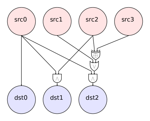
Figure 1: Example system with src and dst nodes connected via binary operations.

The known relationships were used to construct an adjacency matrix where $K_{ij}=1$ indicates that node $i$ is connected to node $j$, with $0$ otherwise. The diagonal is not used as these tautological relationships will provide a perfect score with every metric without providing any new information about the metric’s accuracy or effectiveness. Each metric is applied to every pair of nodes to construct an estimated adjacency matrix $E$. Each element $E_{ij}$ is compared with $K_{ij}$ to give an amount of True-Positive (TP) and False-Negative (FN) where $K_{ij}=1$ or an amount of True-Negative (TN) and False-Positive (FP) where $K_{ij}=0$. For example if a connection is known to exist ($K_{ij}=1$) and the metric calculated a value of $0.7$ then the True-Positive and False-Negative values would be $0.7$ and $0.3$ respectively, with both True-Negative and False-Positive equal to $0$. Alternatively if a connection is know to not exist ($K_{ij}=0$) then True-Negative and False-Positive would be $0.3$ and $0.7$, with True-Positive and False-Negative equal to $0$. These are used to construct the confusion matrix and subsequently give scores for the True Positive Rate (Sensitivity) (TPR), True Negative Rate (Specificity) (TNR), Positive Predictive Value (Precision) (PPV), Negative Predictive Value (NPV), Accuracy (ACC), Balanced Accuracy (BACC), Book-Maker’s Informedness (BMI), and Matthews Correlation Coefficient (MCC). TP $\displaystyle=\sum_{i,j}{\min}{\left(K_{ij},E_{ij}\right)}$ FP $\displaystyle=\sum_{i,j}{\min}{\left(1-K_{ij},E_{ij}\right)}$ TPR $\displaystyle=\frac{\text{TP}}{\text{TP}+\text{FN}}$ PPV $\displaystyle=\frac{\text{TP}}{\text{TP}+\text{FP}}$ ACC $\displaystyle=\frac{\text{TP}+\text{TN}}{\text{TP}+\text{FN}+\text{TN}+\text{FP}}$ FN $\displaystyle=\sum_{i,j}{\min}{\left(K_{ij},1-E_{ij}\right)}$ TN $\displaystyle=\sum_{i,j}{\min}{\left(1-K_{ij},1-E_{ij}\right)}$ TNR $\displaystyle=\frac{\text{TN}}{\text{TN}+\text{FP}}$ NPV $\displaystyle=\frac{\text{TN}}{\text{TN}+\text{FN}}$ BACC $\displaystyle=\frac{\text{TPR}+\text{TNR}}{2}$ BMI $\displaystyle=\text{TPR}+\text{TNR}-1$

$\displaystyle\begin{aligned} \text{MCC}&=\frac{\text{TP}\times\text{TN}-\text{TP}\times\text{TN}}{\sqrt{(\text{TP}+\text{FP})(\text{TP}+\text{FN})(\text{TN}+\text{FP})(\text{TN}+\text{FN})}}\end{aligned}$

To create the dataset $1000$ systems were generated, with $10000$ samples of each node taken from each system. This procedure was repeated for each metric for each system and the PDF of each metric’s accuracy is plotted using Kernel Density Estimation (KDE) to see an overview of how well each performs over a large number of different systems.

5 Results and Discussion

The metrics defined in sec:metrics function as binary classifiers therefore it is reasonable to compare their effectiveness using some of the statistics common for binary classifiers noted above. The TPR measures the proportion of connections which are correctly estimated and the TNR similarly measures the proportion of non-connections correctly estimated. The PPV and NPV measures the proportion of estimates which are correctly estimated to equal the known connections and non-connections. ACC measures the likelihood of an estimation matching a known connection or non-connection. For imbalanced data sets ACC is not necessarily a good way of scoring the performance of these metrics as it may give an overly optimistic score. Normalizing TP and TN by the numbers of samples gives the Balanced Accuracy [16] which may provide a better score for large systems where the adjacency matrices are sparse. Matthews Correlation Coefficient finds the covariance between the known and estimated adjacency matrices which may also be interpreted as a useful score of metric performance. Youden’s J statistic, also known as Book-Maker’s Informedness similarly attempts to capture the performance of a binary classifier by combining the sensitivity and specifitiy to give the probability of an informed decision.

Each statistic was calculated for each metric for each system. Given the large number of systems of various types, PDFs of these statistics are shown in fig:results1 where more weight on the right hand side towards $1.0$ indicates a better metric.

fig:relest_all_TPR shows that $\operatorname{\dot{C}ov}$ and $\operatorname{\dot{D}ep}$ correctly identify the existence of around $25\%$ of existing connections and other metrics identify many more connections. However, fig:relest_all_TNR shows that $\operatorname{\dot{C}ov}$ and $\operatorname{\dot{D}ep}$ are much more likely to correctly identify non-connections than other metrics, especially $\operatorname{\dot{H}am}$ and $\operatorname{\dot{C}ov}$.

For a metric to be considered useful for detecting connections the expected value of both PPV and NPV must be greater than $0$, and ACC must be greater than $0.5$. It can be seen in fig:relest_all_NPV that all metrics score highly for estimating negatives; I.e. when a connection does not exist they give a result close to $0$. On its own this does not carry much meaning as a constant $0$ will always give a correct answer. Similarly, a constant $1$ will give a correct answer for positive links so the plots in the middle and right columns must be considered together with the overall accuracy to judge the usefulness of a metric.

Given that ACC is potentially misleading for imbalanced data sets such as this one it is essential to check against BACC. $\operatorname{\dot{H}am}$ usually has ACC of close to $0.5$ which alone indicates than it is close to useless for detecting connections in binary SoC data. The wider peaks of $\operatorname{\dot{C}os}$ and $\operatorname{\dot{T}mt}$ in both ACC and BACC indicate that these metrics are much more variable in their performance than the likes of $\operatorname{\dot{C}ls}$, $\operatorname{\dot{C}ov}$, and $\operatorname{\dot{D}ep}$. In this pair of plots where $\operatorname{\dot{C}ov}$ and $\operatorname{\dot{D}ep}$ both have much more weight towards the right hand side this indicates that these metrics are more likely to give a good estimate of connectedness.

Finally, using fig:relest_all_MCC and fig:relest_all_BMI as checks it can be see again that $\operatorname{\dot{C}ov}$ and $\operatorname{\dot{D}ep}$ outperform the other metrics. MCC actually has an interval of $[-1,1]$ though the negative side is not plotted here, and given that all all metrics have weight on the positive side this shows that all of the defined metrics contain at least some information on the connectedness.

The overall results indicate that $\operatorname{\dot{H}am}$, $\operatorname{\dot{T}mt}$, $\operatorname{\dot{C}os}$ and $\operatorname{\dot{C}ls}$ are close to useless for detecting connections in datasets resembling the SoC data model described above.

A characteristic feature employed by both $\operatorname{\dot{T}mt}$ and $\operatorname{\dot{C}os}$ is the convolution $f_{x}*f_{y}$, whereas $\operatorname{\dot{H}am}$ and $\operatorname{\dot{C}ls}$ employ an absolute difference $\left|f_{x}-f_{y}\right|$. The best performing metrics $\operatorname{\dot{C}ov}$ and $\operatorname{\dot{D}ep}$ have consistently higher accuracy scores and employ both the convolution, and the product of expectations ${\operatorname{\mathbb{E}}}{\left[f_{x}\right]}{\operatorname{\mathbb{E}}}{\left[f_{y}\right]}$.

The simplicity of these metrics allows hints about the system function to be found quickly in an automated manner, albeit without further information about the formulation or complexity of the relationships. Any information which can be extracted from a dataset about the workings of its system may be used to ease the work of a SoC designer. For example, putting the results into a suitable visualization provides an easy to consume presentation of how related a set of measurements are during a given time window. This allows the SoC designer to make a more educated choice about the set of design parameters in order to provide a more optimal design for their chosen market.

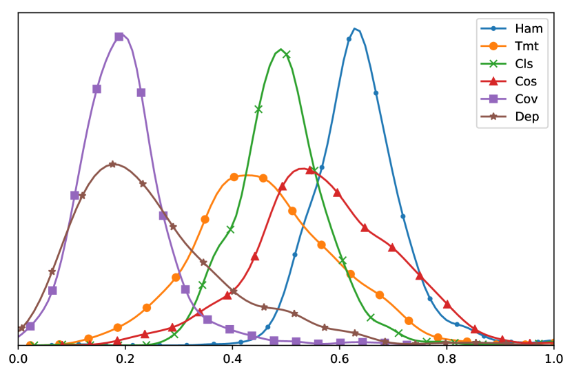
(a) True Positive Rate (Sensitivity).

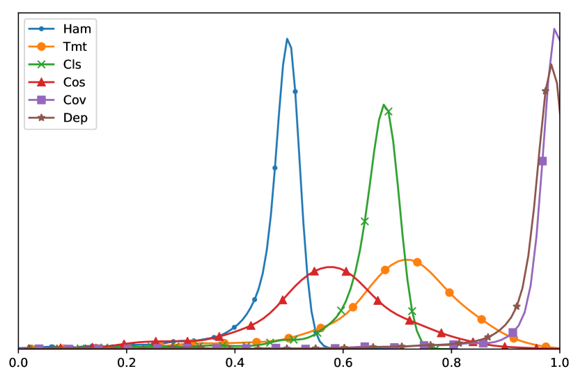
(b) True Negative Rate (Specificity).

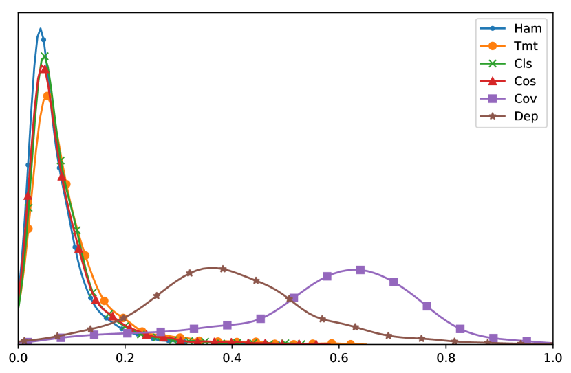
(c) Positive Predictive Value (Precision).

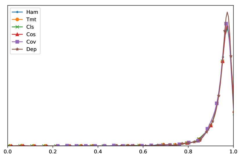
(d) Negative Predictive Value.

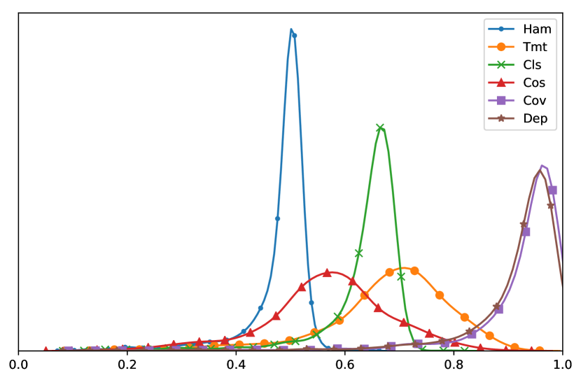
(e) Accuracy.

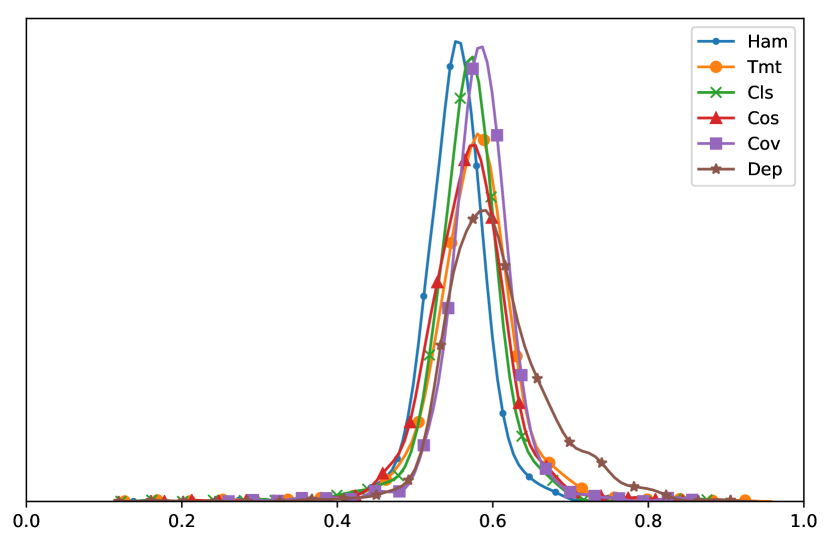
(f) Balanced Accuracy.

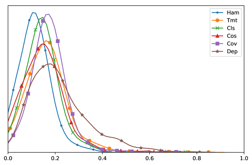
(g) Book-Maker’s Informedness.

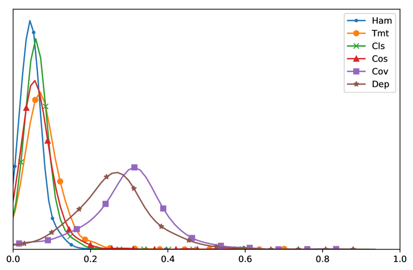
(h) Matthews Correlation Coefficient.

Figure 2: KDE plots of score PDF s averaged across all system types. More weight on the right hand side is always better.

6 Conclusion

The formulation and rationale behind six methods of measuring similarity or correlation to estimate relationships between weighted bit vectors has been given. The given formulations may also be applied more generally to bounded data in the range $[0,1]$, though this is not explored in this paper and may be the subject of future work. Other directions of future work include testing and comparing additional metrics or designing specialized metrics for .

It has been shown that using methods which are common in other fields such as the Hamming distance, Tanimoto distance, Euclidean distance, or Cosine similarity are not well suited to low-cost relationship detection when the relationships are potentially complex. This result highlights a potential pitfall of not considering the system construction for data scientists working with related binary data streams.

The metrics $\operatorname{\dot{C}ov}$ and $\operatorname{\dot{D}ep}$ are shown to consistently estimate the existance of relationships in SoC-like data with higher accuracy than the other metrics. This result gives confidence that detection systems may employ these approaches in order to make meaningful gains in the process of optimizing SoC behavior. By using more accurate metrics unknown relationships may be uncovered giving SoC designer the information they need to optimize their designs and sharpen their competitive edge.

The Python code used to perform the experiments is available online[13].

References

- [1] Choi, S.S., Cha, S.H., Tappert, C.C.: A survey of binary similarity and distance measures. Systems, Cybernetics and Informatics 8(1), 43–48 (2010)
- [2] Frey, B.J., Dueck, D.: Clustering by passing messages between data points. Science 315, 972–976 (1950)
- [3] Friedman, C., Sandow, S.: Learning probabilistic models: An expected utility maximization approach. Journal of Machine Learning Research 4 (Jul 2003)
- [4] Friston, K., Parr, T., Zeidman, P.: Bayesian model reduction. The Wellcome Centre for Human Neuroimaging, Institute of Neurology, London (2018), https://arxiv.org/pdf/1805.07092.pdf
- [5] Gheradi, M., Rotondo, P.: Measuring logic complexity can guide pattern discovery in empirical systems. Complexity 21(S2), 397–408 (Sep 2018)
- [6] Hamming, R.W.: Error detecting and error correcting codes. The Bell System Technical Journal 29(2), 147–160 (1950)
- [7] Ivanovic, M., Kurbalija, V.: Time series analysis and possible applications. 39th International Convention on Information and Communication Technology, Electronics and Microelectronics pp. 473–479 (2016). https://doi.org/10.1109/MIPRO.2016.7522190
- [8] Jaccard, P.: The distribution of the flora in the alpine zone. The New Phytologist 11(2), 37–50 (Feb 1919), http:nph.onlinelibrary.wiley.com/doi/abs/10.1111/j.1469-8137.1912.tb05611.x
- [9] Lagraa, S.: New MP-SoC profiling tools based on data mining techniques. Ph.D. thesis, L’Université de Grenoble (2014), https://tel.archives-ouvertes.fr/tel-01548913
- [10] Lo, D., Khoo, S.C., Liu, C.: Mining past-time temporal rules from execution traces. ACM Workshop On Dynamic Analysis pp. 50–56 (Jul 2008)
- [11] Loo, G.V.: BCM2836 ARM Quad-A7 (2014), https://www.raspberrypi.org/documentation/hardware/raspberrypi/bcm2836/QA7_rev3.4.pdf
- [12] MacKay, D.J.C.: Information Theory, Inference and Learning Algorithms. Cambridge University Press (2002)
- [13] McEwan, D.: relest: Relationship estimation (2019), https://github.com/DaveMcEwan/dmppl/blob/master/dmppl/experiments/relest.py
- [14] McEwan, D., Hlond, M., Nunez-Yanez, J.: Visualizations for understanding SoC behaviour. In: 2019 15th Conference on Ph.D Research in Microelectronics and Electronics (PRIME) (Jul 2019). https://doi.org/10.1109/PRIME.2019.8787837, https://arxiv.org/abs/1905.06386
- [15] Mikolov, T., Chen, K., Corrado, G., Dean, J.: Efficient estimation of word representations in vector space. arXiv e-prints p. arXiv:1301.3781 (Jan 2013)
- [16] Mower, J.P.: PREP-Mt: predictive RNA editor for plant mitochondrial genes. BMC Bioinformatics 6(96) (Apr 2005)
- [17] Rahutomo, F., Kitasuka, T., Aritsugi, M.: Semantic cosine similarity. In: Proceedings of the 7th ICAST 2012, Seoul (Oct 2012)
- [18] Rodgers, J.L., Nicewander, W.A.: Thirteen ways to look at the correlation coefficient. The American Statistitian pp. 59–66 (Feb 1988)
- [19] Rogers, D.J., Tanimoto, T.T.: A computer program for classifying plants. Science 132(3434), 1115–1118 (Oct 1960), http://science.sciencemag.org/content/132/3434/1115/tab-pdf
- [20] Tkacik, G., Bialek, W.: Information processing in living systems. Complexity 21(S2), 397–408 (Sep 2018)