On the Clique-Width of Unigraphs

Abstract

Clique-width is a well-studied graph parameter. For graphs of bounded clique-width, many problems that are NP-hard in general can be polynomial-time solvable. The fact motivates several studies to investigate whether the clique-width of graphs in a certain class is bounded or not. We focus on unigraphs, that is, graphs that are uniquely determined by their degree sequences up to isomorphism. We show that every unigraph has clique-width at most 4. It follows that many problems that are NP-hard in general are polynomial-time solvable for unigraphs.

1 Introduction

Clique-width is a well-studied graph parameter [8]. Clique-width can be seen as a generalization of another well-known graph parameter, treewidth. If the treewidth of a graph is a constant, its clique-width is a constant [7]. The converse is not true in general. For example, the complete graph with $n$ vertices has the treewidth $n$ but the clique-width 2 regardless of $n$. As shown in this example, clique-width can be bounded by a constant even for dense graphs, unlike treewidth. If the clique-width of a graph class is bounded, many problems that are NP-hard in general can be polynomial-time solvable for the class [9, 20, 24]. The fact motivates several studies to show that the clique-width of some graph classes are bounded [10, 13] and that of others are not [13, 3].

As a graph class whose clique-width is not known to be bounded, we focus on unigraphs [17, 21], that is, graphs uniquely determined by their degree sequences up to isomorphism. Unigraphs include important graph classes such as threshold graphs [5], split matrogenic graphs [14], matroidal graphs [23], and matrogenic graphs [12]. For all these subclasses, it is known that the clique-width is at most 4 [9]. However, it is open for unigraphs. We think that there are two main reasons for the difference. First, although all the subclasses are hereditary, that is, closed under taking induced subgraphs, unigraphs are not as shown in Fig. 1. It makes the analysis of unigraphs difficult. Second, although there are many graph-theoretic studies for unigraphs, there are few algorithmic ones. Analyzing the clique-width of unigraphs is important to reveal algorithmic aspects of unigraphs.

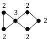
(a) Unigraph $G$.

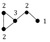
(b) Induced subgraph $F$ of $G$.

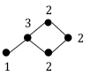
(c) Graph that has the same degree sequence $(3,2,2,2,1)$ as $F$ but is not isomorphic to $F$.

Figure 1: Examples to show that unigraphs are not hereditary. The number beside a vertex is its degree.

In this paper, we show that the clique-width of unigraphs is at most 4. It follows that many problems that are NP-hard in general are polynomial-time solvable for unigraphs. We prove our result by a relationship between clique-width and the characterization of unigraphs based on the canonical decomposition of graphs given by Tyshkevich [25].

This paper is organized as follows. The rest of this section summarizes related work. Section 2 gives preliminaries on graphs (Section 2.1), clique-width (Section 2.2), and the canonical decomposition of graphs and the characterization of unigraphs (Section 2.3). In Section 3, we show our main result: the clique-width of unigraphs is at most 4.

Related Work.

Clique-width is introduced by Courcelle et al. [8]. Although calculating the clique-width of a graph is NP-hard in general [11], whether the clique-width of a graph is at most 3 or not can be determined in polynomial time [6]. By Courcelle’s theorem, every problem can be written in so-called MSO₁ admits a linear-time algorithm for graphs of bounded clique-width [9]. These problems include Clique, Vertex Cover, and Dominating Set. Our result implies that all such problems are linear-time solvable for unigraphs. Clique-width is related to other graph parameters than treewidth. For example, clique-width is constant if and only if rank-width [22] or NLC-width [16] is constant. Our result indicates that both the parameters are bounded for unigraphs. For some graph classes, whether the clique-width of the class is bounded by a constant or not is studied. For example, cographs are exactly the graphs with clique-width at most 2 [10] and the clique-width of distance-hereditary graphs is at most 3 [13]. In contrast, the clique-width is unbounded for unit interval graphs [13] and bipartite permutation graphs [3].

Unigraphs and its subclasses are well-studied [17, 21, 14, 5, 23, 12]. Although they are intensively studied from a graph-theoretic view, there are a few studies from an algorithmic view. As a few examples, there are linear-time recognition algorithms for unigraphs [1, 19]. Calamoneri and Petreschi [4] give an approximation algorithm for $L(2,1)$-labeling, a variant of graph coloring, of unigraphs. However, it is open whether the problem is NP-hard for unigraphs. Since, $L(2,1)$-labeling can be written in MSO₁ [4], our result implies that we can decide whether there exists an $L(2,1)$-labeling using $\ell$ colors for a fixed value of $\ell$ in linear time for unigraphs. In contrast, it is still open whether $L(2,1)$-labeling for not fixed $\ell$ can be polynomial-time solvable for unigraphs.

Graphs with few $P_{4}$’s, i.e., $P_{4}$-sparse graphs and partner-limited graphs, are known to have clique-width at most 4 [18]. Unigraphs are not contained in these classes since the double star $S_{2}(p,2)$ (see Section 2.3) is a counterexample.

2 Preliminaries

2.1 Graphs

Let $G$ be a graph. We assume that $G$ is connected and simple (without self-loops and multi-edges). $V(G)$ and $E(G)$ denotes the vertex and edge sets of $G$, respectively. The subgraph induced by $V^{\prime}\subseteq V(G)$ is denoted by $G[V^{\prime}]$. If $G[V^{\prime}]$ is a complete graph, $V^{\prime}$ is a clique. If $G[V^{\prime}]$ has no edges, $V^{\prime}$ is an independent set. $\overline{G}$ denotes the complement graph of $G$. $K_{n}$, $P_{n}$, and $C_{n}$ denotes the complete, path, and cycle graph with $n$ vertices, respectively. $K_{n,m}$ denotes the complete bipartite graph with the two parts of $n$ and $m$ vertices. Especially, $K_{1,n}$ is a star; its center is the vertex with degree $n$ (when $n=1$, we choose an arbitrary vertex of $K_{1,1}$), and its leaves are the other vertices. For graphs $G$ and $H$ with $V(G)\cap V(H)=\emptyset$, their disjoint union is the graph $G\oplus H=(V(G)\cup V(H),E(G)\cup E(H))$. We define $mK_{2}$ as the disjoint union of $m$ copies of $K_{2}$. For a positive integer $k$, we define $[k]=\left\{1,\dots,k\right\}$.

A graph $G$ is a split graph if $V(G)$ can be partitioned into two sets $A$ and $B$ such that $A$ is a clique and $B$ is an independent set. A graph $G$ is a unigraph if it is uniquely determined by its degree sequence up to isomorphism. A graph class $\mathcal{G}$ is hereditary if, for every graph $G\in\mathcal{G}$, all induced subgraphs of $G$ are also in $\mathcal{G}$. Unigraphs are not hereditary. For example, although the graph in Fig. 1(a) is a unigraph, there is an induced subgraph that is not a unigraph (Figs. 1(b) and 1(c)).

2.2 Clique-Width

Definition 1 (Clique-width).

For a graph $G$, its clique-width $\mathrm{cw}(G)$ is the minimum number of labels needed to construct $G$ by the following four operations:

• $v(i):$ introduce a new vertex $v$ with label $i$.

• $\oplus:$ given two graphs $G$ and $H$, take their disjoint union $G\oplus H$.

• $\eta_{i,j}\,(i\neq j):$ add edges between every two vertices with label $i$ and $j$.

• $\rho_{i\rightarrow j}:$ for all vertices with label $i$, change the labels into $j$.

The procedure to construct a graph $G$ by the above four operations can be associated with an algebraic expression. Such an expression using at most $k$ labels is a $k$-expression. A tree associated with a $k$-expression is the $k$-expression tree. Fig. 2 shows a $3$-expression tree for the graph in Fig. 1(a).

Cographs are exactly the graphs with clique-width at most 2 [10]. In addition, a graph is a cograph if and only if it is $P_{4}$-free [2]. Since a complement graph of a cograph is also a cograph [2], the following lemma holds.

Lemma 1.

If a graph $G$ is $P_{4}$-free, both $\mathrm{cw}(G)$ and $\mathrm{cw}(\overline{G})$ are at most 2.

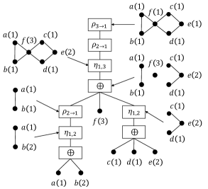
Figure 2: $3$-expression tree for the graph in Fig. 1(a). Each graph corresponds to the subtree rooted at the node pointed at by the arrow. $v(i)$ means that a vertex $v$ has the label $i$. The $3$-expression corresponding to the tree is $\rho_{3\rightarrow 1}\rho_{2\rightarrow 1}\eta_{1,3}(\rho_{2\rightarrow 1}\eta_{1,2}(a(1)\oplus b(2))\oplus f(3)\oplus\eta_{1,2}(c(1)\oplus d(1)\oplus e(2)))$.

2.3 Canonical Decomposition and Characterization of Unigraphs

In this subsection, we introduce the canonical decomposition of Tyshkevich [25] and a characterization of unigraphs.

Definition 2 (Splitted graph).

Let $G$ be a split graph with a bipartition $V(G)=A\cup B$, where $A$ is a clique and $B$ is an independent set. The triple $(G,A,B)$ is a splitted graph.

Definition 3 (Composition).

Let $(G,A,B)$ be a splitted graph and $H=(V(H),E(H))$ be a simple graph. Their composition is the graph $F=(G,A,B)\circ H$ such that:

• $V(F)=A\cup B\cup V(H)$, and

• $E(F)=E(G)\cup E(H)\cup\left\{\left\{a,v\right\}\;\middle|\;a\in A,v\in V(H)\right\}$.

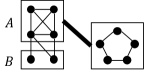
(a) $G\circ H$.

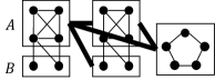
(b) $G\circ G\circ H$.

Figure 3: Compositions of graphs. A bold line indicates that all the vertices in the endpoints are adjacent.

Intuitively, $(G,A,B)\circ H$ is a graph obtained by adding edges between every vertex in $A$ and $V(H)$ in $G\oplus H$. Fig. 3 shows examples of compositions. Note that a composition of two splitted graphs can be regarded as a splitted graph. For two splitted graphs $(G_{1},A_{1},B_{1})$ and $(G_{2},A_{2},B_{2})$, their composition can be written as $(G,A_{1}\cup A_{2},B_{1}\cup B_{2})$. Since the operation $\circ$ is associative, we omit parentheses when we use $\circ$ multiple times. If a graph can be written as $(G,A,B)\circ H$, the graph is decomposable; otherwise, indecomposable.

Theorem 2.1 (Decomposition theorem [25]).

Every graph $G$ can be uniquely decomposed as $G=(G_{k},A_{k},B_{k})\,\circ\,\dots\,\circ\,(G_{1},A_{1},B_{1})\,\circ\,G_{0}$, where $(G_{i},A_{i},B_{i})\,(i\in[k])$ is an indecomposable split graph and $G_{0}$ is an indecomposable nonsplit graph.

For a graph $G$, we call $(G_{k},A_{k},B_{k})\circ\dots(G_{1},A_{1},B_{1})\circ G_{0}$ the canonical decomposition of $G$. Tyshkevich gives a characterization of unigraphs based on Theorem 2.1. To explain it, we need some additional definitions. For a splitted graph $(G,A,B)$, its complement $\overline{(G,A,B)}$ is $(\overline{G},B,A)$ and inverse ${(G,A,B)^{I}}$ is $({G^{I}},B,A)$, where $\overline{G}$ is a complement graph of $G$ and ${G^{I}}$ is the graph obtained by removing the edges in $\left\{\{a_{1},a_{2}\}\;\middle|\;a_{1},a_{2}\in A\right\}$ from $G$ and then adding the edges in $\left\{\{b_{1},b_{2}\}\;\middle|\;b_{1},b_{2}\in B\right\}$ to $G$. In other words, ${G^{I}}$ is the graph obtained from $G$ by inverting the existence of edges in the clique and the independent set.

We define the following graphs:

• $U_{2}(m,s)$: It is the disjoint union of $mK_{2}\,(m\geq 1)$ and $K_{1,s}\,(s\geq 2)$. (Fig. 4(a))

• $U_{3}(m)$: For $m\geq 1$, the graph is obtained by taking the disjoint union of $C_{4}$ and $m$ triangles $K_{3}$, choosing a vertex from each component, and merging all the vertices into one. (Fig. 4(b))

• $S_{2}(p_{1},q_{1};\dots;p_{t},q_{t})$: For each $i\in[t]$, take the disjoint union of $q_{i}$ stars $K_{1,p_{i}}$ and add edges connecting every two centers of the stars, where $p_{i},q_{i},t\geq 1$ and $q_{1}+\dots+q_{t}\geq 2$. (Fig. 5(a))

• $S_{3}(p,q_{1};q_{2})$: For $S_{2}(p,q_{1};p+1,q_{2})$, where $p\geq 1,q_{1}\geq 2$ and $q_{2}\geq 1$, add a new vertex $v$ into the independent set and connect $v$ with the centers of $K_{1,p}$. (Fig. 5(b))

• $S_{4}(p,q)$: For $S_{3}(p,2;q)$, where $q\geq 1$, add a new vertex $u$ into the clique and connect $u$ with all the vertices other than $u$ and $v$. (Fig. 5(c))

Theorem 2.2 (Characterization of unigraphs [25]).

Unigraphs are the graphs can be written as $(G_{k},A_{k},B_{k})\circ\dots\circ(G_{1},A_{1},B_{1})\circ G_{0}$, where:

• $k\geq 0$ if $G_{0}\neq\emptyset$ and $k\geq 1$ otherwise;

• For each $i\in[k]$, either $G_{i}$, $\overline{G_{i}}$, ${G_{i}^{I}}$, or $\overline{{G_{i}^{I}}}$ is one of the following split unigraphs:

  $$K_{1},\quad S_{2}(p_{1},q_{1};\dots;p_{t},q_{t}),\quad S_{3}(p,q_{1};q_{2}),\quad S_{4}(p,q);$$ (1)

• If $G_{0}\neq\emptyset$, either $G_{0}$ or $\overline{G_{0}}$ is one of the following nonsplit unigraphs:

  $$C_{5},\quad mK_{2}\ (m\geq 2),\quad U_{2}(m,s),\quad U_{3}(m).$$ (2)

(a) $U_{2}(m,s)$.

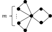
(b) $U_{3}(m)$.

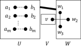
(c) $\overline{U_{3}(m)}$. In $U$, two vertices are adjacent if and only if the vertices are not joined by a dotted line. The bold line indicates that all the vertices in $U$ and $W$ are adjacent each other.

Figure 4: Indecomposable nonsplit unigraphs.

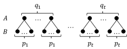
(a) $S_{2}(p_{1},q_{1};\dots;p_{t},q_{t})$.

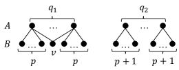
(b) $S_{3}(p,q_{1};q_{2})$.

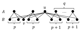
(c) $S_{4}(p,q)$.

Figure 5: Indecomposable split unigraphs. In each figure, the upper part is a clique and the lower part is an independent set. The edges connecting the vertices in the clique are omitted.

3 Clique-Width of Unigraphs

In this section, we show that the clique-width of unigraphs is at most 4. We prove our result by focusing on a relationship between Theorem 2.2 and the clique-width.

Definition 4 (Split labeling).

A splitted graph $(G,A,B)$ is split labeled if all the vertices in the clique $A$ have the label $1$ and all the vertices in the independent set $B$ have the label $2$.

Definition 5 (Split clique-width).

For a splitted graph $(G,A,B)$, its split clique-width $\mathrm{scw}(G)$ is the minimum number of labels needed to split label $G$ by the four operations in Definition 1. In addition, the $k$-split expression is a $k$-expression to split label $G$ with at most $k$ labels and the $k$-split expression tree is the corresponding expression tree.

In the following, when the clique-width of $G$ is at most $k$, we use $\epsilon[G,k]$ to denote an arbitrary $k$-expression of $G$. (We assume that the labels of all vertices are 1 after evaluating $\epsilon[G,k]$.) In addition, when the split clique-width of a splitted graph $(G,A,B)$ is at most $k$, we use $\sigma[G,k]$ to denote an arbitrary $k$-split expression of $G$.

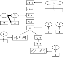
(a) Split expression tree imitating the composition of splitted graphs.

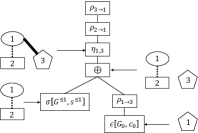
(b) Expression tree imitating the composition of a splitted graph and a simple graph.

Figure 6: Expression trees imitating compositions of graphs. An ellipse is a clique and a square is an independent set. A pentagon is a simple graph. A bold line indicates that all the vertices in the endpoints are adjacent and a dotted line indicates that arbitrarily adjacent.

Lemma 2.

Let $G$ and $(G_{k},A_{k},B_{k})\circ\dots\circ(G_{1},A_{1},B_{1})\circ G_{0}$ be a unigraph and its canonical decomposition, respectively. Then,

$$\mathrm{cw}(G)\leq\max\left\{4,\max_{i\in[k]}\mathrm{scw}(G_{i}),\mathrm{cw}(G_{0})\right\}.$$ (3)

Proof.

Let $c_{0}=\mathrm{cw}(G_{0})$, $s_{i}=\mathrm{scw}(G_{i})$, and $G^{\leq i}=G_{k}\circ\dots\circ G_{i}$ for each $i\in[k]$. Since a composition of splitted graphs can be regarded as a splitted graph, $G_{i}$ is a splitted graph for each $i\in[k]$. Thus, we define $s^{\leq i}=\mathrm{scw}(G^{\leq i})$ for each $i\in[k]$. If $k=0$ ($G=G_{0}$), then $\mathrm{cw}(G)=c_{0}$, and thus (3) holds. We assume $k>0$ in the following.

For each $i\in[k]$, we show the following by induction:

$$s^{\leq i}\leq\max\left\{4,\max_{i\leq j\leq k}s_{j}\right\}.$$ (4)

First, by definition, $s^{\leq k}\leq s_{k}$ holds. Next, for an integer $i$ with $2\leq i\leq k$, assume that (4) holds. Then, we can construct a split expression of $G^{\leq i-1}=G^{\leq i}\circ G_{i-1}$ using $\sigma[G^{\leq i},s^{\leq i}]$ and $\sigma[G_{i-1},s_{i-1}]$:

$$\rho_{4\rightarrow 2}\,\rho_{3\rightarrow 1}\,\eta_{1,4}\,\eta_{1,3}\left(\sigma[G^{\leq i},s^{\leq i}]\oplus\rho_{2\rightarrow 4}\,\rho_{1\rightarrow 3}\,\sigma[G_{i-1},s_{i-1}]\right).$$ (5)

Fig. 6(a) shows the corresponding split expression tree. The number of labels used in (5) is (including the labels inside $\sigma[G^{\leq i},s^{\leq i}]$ and $\sigma[G_{i-1},s_{i-1}]$):

$$\max\left\{4,s^{\leq i},s_{i-1}\right\} \leq\max\left\{4,\left\{4,\max_{i\leq j\leq k}s_{j}\right\},s_{i-1}\right\}$$

$$=\max\left\{4,\max_{i-1\leq j\leq k}s_{j}\right\}.$$ (6)

Therefore, (4) holds for $i-1$. By induction, (4) holds also for $i=1$. If $G_{0}=\emptyset$, we have proven (3). If $G_{0}\neq\emptyset$, we can construct a split expression of $G=G^{\leq 1}\circ G_{0}$ using $\sigma[G^{\leq 1},s^{\leq 1}]$ and $\epsilon[G_{0},c_{0}]$:

$$\rho_{3\rightarrow 1}\rho_{2\rightarrow 1}\,\eta_{1,3}\left(\sigma[G^{\leq 1},s^{\leq 1}]\oplus\rho_{1\rightarrow 3}\,\epsilon[G_{0},c_{0}]\right).$$ (7)

Fig. 6(b) shows the corresponding expression tree. The number of labels used in (7) is (including the labels inside $\sigma[G^{\leq 1},s^{\leq 1}]$ and $\epsilon[G_{0},c_{0}]$):

$$\max\left\{3,s^{\leq 1},c_{0}\right\} \leq\max\left\{3,\left\{4,\max_{i\in[k]}s_{i}\right\},c_{0}\right\}$$

$$=\max\left\{4,\max_{i\in[k]}s_{i},c_{0}\right\}.$$ (8)

Therefore, (3) holds. ∎∎

By Lemma 2, to prove $\mathrm{cw}(G)\leq 4$, it suffices to show that $\mathrm{cw}(G_{0})$ and $\mathrm{scw}(G_{i})\ (i\in[k])$ are at most 4.

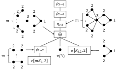
(a) $3$-expression tree for $U_{3}(m)$.

(b) $3$-expression tree for $\overline{U_{3}(m)}$. In $\overline{mK_{2}}$, two vertices are adjacent if and only if they are not joined by a dotted line.

Figure 7: Expression trees for indecomposable nonsplit unigraphs.

Lemma 3.

$\mathrm{cw}(G_{0})\leq 3$.

Proof.

By Theorem 2.2, either $G_{0}$ or $\overline{G_{0}}$ is one of the graphs in (2). We show the clique-widths of the graphs in (2) and their complement graphs are at most 4. Table 1 in Appendix 0.A summarizes the results shown in the below.

The clique-width of $C_{5}\ (=\overline{C_{5}})$ is exactly 3 [10]. Since $mK_{2}$ and $U_{2}(m,s)$ are $P_{4}$-free, by Lemma 1, all of $\mathrm{cw}(mK_{2})$, $\mathrm{cw}(U_{2}(m,s))$, $\mathrm{cw}(\overline{mK_{2}})$, and $\mathrm{cw}(\overline{U_{2}(m,s)})$ are at most 2.

Next, we consider $U_{3}(m)$. We can construct a $3$-expression of $U_{3}(m)$ using $\epsilon[mK_{2},2]$ and $\sigma[K_{1,2},2]$:

$$\rho_{3\rightarrow 1}\,\rho_{2\rightarrow 1}\,\eta_{2,3}\left(\rho_{1\rightarrow 2}\,\epsilon[mK_{2},2]\oplus v(3)\oplus\sigma[K_{1,2},2]\right).$$ (9)

Therefore, $\mathrm{cw}(U_{3}(m))\leq 3$. Fig. 7(a) shows a $3$-expression tree corresponding to the $3$-expression in (9).

Finally, we consider $\overline{U_{3}(m)}$, which is shown in Fig. 4(c). The vertex set can be partitioned into three sets $U=\left\{a_{1},b_{1},\dots,a_{m},b_{m}\right\}$, $V=\left\{v\right\}$, and $W=\left\{w_{1},w_{2},w_{3}\right\}$. The edge set is $\left\{\left\{a_{i},b_{j}\right\}\;\middle|\;i\neq j\right\}\cup\left\{\left\{u,w\right\}\;\middle|\;u\in U,w\in W\right\}\cup\left\{\left\{v,w_{2}\right\},\left\{w_{1},w_{3}\right\}\right\}$. Observe that $\overline{U_{3}(m)}[U]$ is isomorphic to $\overline{mK_{2}}$ and $\overline{U_{3}(m)}[W]$ is isomorphic to $K_{2}\oplus K_{1}$. Therefore, the following $3$-expression constructs $\overline{U_{3}(m)}$:

$$\rho_{3\rightarrow 1}\,\rho_{2\rightarrow 1}\,\eta_{1,2}\left(\begin{array}[]{c}\epsilon[\overline{mK_{2}},2]\\ \oplus\\ \rho_{1\rightarrow 2}\,\eta_{2,3}\,\left(v(3)\oplus\sigma[K_{2}\oplus K_{1},2]\right)\end{array}\right).$$ (10)

It follows that $\mathrm{cw}(\overline{U_{3}(m)})\leq 3$. Fig. 7(b) shows the corresponding $3$-expression tree to the $3$-expression in (10). ∎∎

Lemma 4.

For each $i\in[k]$, $\mathrm{scw}(G_{i})\leq 4$.

Proof.

By Theorem 2.2, for each $i\in[k]$, either $G_{i},\overline{G_{i}},{G_{i}^{I}}$, or $\overline{{G_{i}^{I}}}$ is one of the graphs in (1). We show that the clique-width of each graph is at most 4. Note that, when either $G_{i}$, $\overline{G_{i}}$, ${G_{i}^{I}}$, or $\overline{{G_{i}^{I}}}$ is $K_{1}$, it is easy to split label it by one label. When the splitted graph is $(K_{1},\left\{a\right\},\emptyset)$ (resp. $(K_{1},\emptyset,\left\{a\right\})$), we introduce $a$ with label 1 (resp. 2). In the following we consider $S_{2}$, $S_{3}$, and $S_{4}$. First, we show that the clique-width of $S_{2}$, $\overline{S_{2}}$, ${S_{2}^{I}}$, and $\overline{{S_{2}^{I}}}$ are at most 3 or 4 by induction. Next, for $S_{3}$ and $S_{4}$, we construct $4$-split expressions from $S_{2}$. Similarly, we construct $4$-split expressions for $\overline{S_{3}}$ and $\overline{S_{4}}$ from $\overline{S_{2}}$, and the same goes to ${S_{3}^{I}}$, ${S_{4}^{I}}$, $\overline{{S_{3}^{I}}}$, and $\overline{{S_{4}^{I}}}$. Table 2 in Appendix 0.A summarizes the results shown in the below.

The graph $S_{2}$ is obtained by taking disjoint union of $l=\sum_{i=1}^{t}q_{i}$ stars and adding edges between every two centers of the stars. Let $p^{\prime}_{1},\dots,p^{\prime}_{l}$ be the non-decreasing sequence of degrees of the centers of the stars. We write $S_{2}(p_{1},q_{1};\dots;p_{t},q_{t})$ as $S_{2}(p^{\prime}_{1},\dots,p^{\prime}_{l})$. We define $S_{2}^{\leq i}=S_{2}(p^{\prime}_{1},\dots,p^{\prime}_{i})$. For each $i\in[l]$, $S_{2}^{\leq i}$ is a split graph. We show that, for each $i\in[l]$, the split clique-width of $S_{2}^{\leq i}$ is at most 3 by induction. First, $S_{2}^{\leq 1}=K_{1,p^{\prime}_{1}}$ is a star. In general, $K_{1,n}$ is constructed by the following $2$-split expression:

$$\eta_{1,2}\left(u(1)\oplus v_{1}(2)\oplus\dots\oplus v_{n}(2)\right),$$ (11)

where $u$ is the center of the star and $v_{i}\ (i\in[n])$ is a leaf. Next, for an integer $i\in[l-1]$, assume that $\mathrm{scw}(S_{2}^{\leq i})\leq 3$. Then, $S_{2}^{\leq i+1}$ can be constructed by the following $3$-split expression using $\sigma[S_{2}^{\leq i},3]$ and $\sigma[K_{1,p^{\prime}_{i+1}},2]$:

$$\rho_{3\rightarrow 1}\,\eta_{1,3}\left(\sigma[S_{2}^{\leq i},3]\oplus\rho_{1\rightarrow 3}\,\sigma[K_{1,p^{\prime}_{i+1}},2]\right).$$ (12)

Therefore, $\mathrm{scw}(S_{2}^{\leq i+1})\leq 3$. Fig. 8 in Appendix 0.B shows the corresponding expression tree. By induction, $\mathrm{scw}(S_{2}^{\leq l})\leq 3$ holds.

The graph ${S_{2}^{I}}$ is obtained by taking disjoint union of $l$ stars and adding edges between the leaves of the stars. We define ${S_{2}^{I}}^{\leq i}$ in the same way as $S_{2}^{\leq i}$. We show that $\mathrm{scw}({S_{2}^{I}}^{\leq i})\leq 3$ for each $i\in[l]$ by induction. First, ${S_{2}^{I}}^{\leq 1}={K_{1,p^{\prime}_{1}}^{I}}$ is a graph obtained by adding a vew vertex $w$ to $K_{p^{\prime}_{1}}$ and edges between $w$ and the other vertices, that is, $K_{p^{\prime}_{1}+1}$. In general, $K_{n+1}$ is constructed by the following $2$-split expression:

$$\eta_{1,2}\left(w(2)\oplus\epsilon[K_{n},2]\right).$$ (13)

Next, for an integer $i\in[l-1]$, assume that $\mathrm{scw}({S_{2}^{I}}^{\leq i})\leq 3$. Then, ${S_{2}^{I}}^{\leq i+1}$ can be constructed by the following $3$-split expression using $\sigma[{S_{2}^{I}}^{\leq i},3]$ and $\sigma[{K_{1,p^{\prime}_{i+1}}^{I}},2]$:

$$\rho_{3\rightarrow 1}\,\eta_{1,3}\left(\sigma[{S_{2}^{I}}^{\leq i},3]\oplus\rho_{1\rightarrow 3}\,\sigma[{K_{1,p^{\prime}_{i+1}}^{I}},2]\right)$$ (14)

Fig. 9 in Appendix 0.B shows the corresponding expression tree. By induction, $\mathrm{scw}({S_{2}^{I}}^{\leq l})\leq 3$ holds.

The graph $\overline{S_{2}}$ is the following graph. The vertex set can be partitioned into $C=\left\{c_{1},\dots,c_{l}\right\},L_{1},\dots,L_{l}$, where $L_{i}$ contains $p_{i}^{\prime}$ vertices. Two vertices $u$ and $v$ are adjacent if and only if (a) for some integers $i$ and $j$ with $i\neq j$, both $u=c_{i}$ and $v\in L_{j}$ hold, or (b) for some integers $i$ and $j$ (possibly $i=j$), $u\in L_{i}$ and $v\in L_{j}$ hold. For each integer $i\in[l]$, we define $\overline{S_{2}}^{\leq i}$ as an induced subgraph of $\overline{S_{2}}$ by the set $\left\{c_{1},\dots,c_{i}\right\}\cup L_{1}\cup\dots\cup L_{i}$ of vertices. We show that $\mathrm{scw}(\overline{S_{2}}^{\leq i})\leq 4$ for each $i\in[l]$ by induction. First, $\overline{S_{2}}^{\leq 1}$ is the disjoint union of an isolated vertex $c_{1}$ and the complete graph induced by $L_{1}$, that is, $\overline{S_{2}}^{\leq 1}=\overline{K_{1,p^{\prime}_{1}}}=K_{1}\oplus K_{p^{\prime}_{1}}$. In general, $\overline{K_{1,n}}$ is constructed by the following $2$-split expression:

$$u(2)\oplus\epsilon[K_{n},2],$$ (15)

where $u$ is the isolated vertex (the only vertex of $K_{1}$). Next, for an integer $i\in[l-1]$, assume that $\mathrm{scw}(\overline{S_{2}}^{\leq i})\leq 4$. Then, $\overline{S_{2}}^{\leq i}$ is constructed by the following $4$-split expression using $\sigma[\overline{S_{2}}^{\leq i},4]$ and $\sigma[\overline{K_{1,p^{\prime}_{i+1}}},2]$:

$$\rho_{4\rightarrow 2}\,\rho_{3\rightarrow 1}\,\eta_{2,3}\,\eta_{1,4}\,\eta_{1,3}\left(\sigma[\overline{S_{2}}^{\leq i},4]\oplus\rho_{2\rightarrow 4}\,\rho_{1\rightarrow 3}\,\sigma[\overline{K_{1,p^{\prime}_{i+1}}},2]\right).$$ (16)

Fig. 10 in Appendix 0.B shows the corresponding expression tree. By induction, $\mathrm{scw}(\overline{S_{2}}^{\leq l})\leq 4$ holds.

The graph $\overline{{S_{2}^{I}}}$ is the following graph. Similarly to $\overline{S_{2}}$, the vertex set can be partitioned into $C=\left\{c_{1},\dots,c_{l}\right\},L_{1},\dots,L_{l}$. Two vertices $u$ and $v$ are adjacent if and only if (a) for some integers $i$ and $j$ such that $i\neq j$, both $u=c_{i}$ and $v\in L_{j}$ hold, or (b) for some integers $i$ and $j$ (possibly $i=j$), $u,v\in C$ holds. We define $\overline{{S_{2}^{I}}}^{\leq i}$ in the same way as $\overline{S_{2}}^{\leq i}$. We show that $\mathrm{scw}(\overline{{S_{2}^{I}}}^{\leq i})\leq 4$ for each $i\in[l]$ by induction. $\overline{{S_{2}^{I}}}^{\leq 1}$ is the disjoint union of the isolated vertex $c_{1}$ and $|L_{1}|=p_{1}^{\prime}$ isolated vertices, that is, $\overline{{S_{2}^{I}}}^{\leq 1}=\overline{{K_{1,p_{1}^{\prime}}^{I}}}=K_{1}\oplus\overline{K_{p_{1}^{\prime}}}$. In general, $\overline{{K_{1,n}^{I}}}$ is constructed by the following $2$-split expression:

$$u(1)\oplus v_{1}(2)\oplus\dots\oplus v_{n}(2).$$ (17)

Next, for an integer $i\in[l-1]$, assume that $\mathrm{scw}(\overline{{S_{2}^{I}}}^{\leq i})\leq 4$. Then, $\overline{{S_{2}^{I}}}^{\leq i+1}$ is constructed by the following $4$-split expression using $\sigma[\overline{{S_{2}^{I}}}^{\leq i},4]$ and $\sigma[\overline{{K_{1,p^{\prime}_{i+1}}^{I}}},2]$:

$$\rho_{4\rightarrow 2}\,\rho_{3\rightarrow 1}\,\eta_{2,3}\,\eta_{1,4}\,\eta_{1,3}\left(\sigma[\overline{{S_{2}^{I}}}^{\leq i},4]\oplus\rho_{2\rightarrow 4}\,\rho_{1\rightarrow 3}\,\sigma[\overline{{K_{1,p^{\prime}_{i+1}}^{I}}},2]\right).$$ (18)

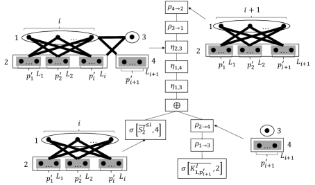
Figure 11: Expression tree for $\overline{{S_{2}^{I}}}$.

Fig. 11 in Appendix 0.B shows the corresponding expression tree. By induction, $\mathrm{scw}(\overline{{S_{2}^{I}}}^{\leq l})\leq 4$.

$S_{3}$, ${S_{3}^{I}}$, $\overline{S_{3}}$, and $\overline{{S_{3}^{I}}}$ are constructed by the following 3, 3, 4, and 4-split expressions, respectively:

$$\rho_{3\rightarrow 1}\,\eta_{1,3}\left(\begin{array}[]{c}\rho_{3\rightarrow 2}\,\eta_{1,3}\left(\sigma[S_{2}(p,q_{1}),3]\oplus v(3)\right)\\ \oplus\\ \rho_{1\rightarrow 3}\,\sigma[S_{2}(p+1,q_{2}),3]\end{array}\right),$$ (19)

$$\rho_{3\rightarrow 1}\,\eta_{1,3}\left(\begin{array}[]{c}\eta_{2,3}\left(\sigma[{S_{2}^{I}}(p,q_{1}),3]\oplus v(3)\right)\\ \oplus\\ \rho_{1\rightarrow 3}\,\sigma[{S_{2}^{I}}(p+1,q_{2}),3]\end{array}\right),$$ (20)

$$\rho_{4\rightarrow 2}\,\rho_{3\rightarrow 1}\,\eta_{2,3}\,\eta_{1,4}\,\eta_{1,3}\left(\begin{array}[]{c}\rho_{3\rightarrow 1}\,\eta_{1,3}\left(\sigma[\overline{S_{2}}(p,q_{1}),4]\oplus v(3)\right)\\ \oplus\\ \rho_{2\rightarrow 4}\,\rho_{1\rightarrow 3}\,\sigma[\overline{S_{2}}(p+1,q_{2}),4]\end{array}\right),$$ (21)

$$\rho_{4\rightarrow 2}\,\rho_{3\rightarrow 1}\,\eta_{2,3}\,\eta_{1,4}\,\eta_{1,3}\left(\begin{array}[]{c}\left(\sigma[\overline{{S_{2}^{I}}}(p,q_{1}),4]\oplus v(2)\right)\\ \oplus\\ \rho_{2\rightarrow 4}\,\rho_{1\rightarrow 3}\,\sigma[\overline{{S_{2}^{I}}}(p+1,q_{2}),4]\end{array}\right).$$ (22)

Therefore, $\mathrm{scw}(S_{3})$, $\mathrm{scw}({S_{3}^{I}})$, $\mathrm{scw}(\overline{S_{3}})$, and $\mathrm{scw}(\overline{{S_{3}^{I}}})$ are at most $3,3,4$, and $4$, respectively.

$S_{4}$, ${S_{4}^{I}}$, $\overline{S_{4}}$, and $\overline{{S_{4}^{I}}}$ are constructed by the following 4-split expressions:

$$\rho_{4\rightarrow 2}\,\rho_{3\rightarrow 1}\,\eta_{2,3}\,\eta_{1,3}\left(u(3)\oplus X_{1}\right),$$ (23)

$$\rho_{4\rightarrow 2}\,\rho_{3\rightarrow 1}\,\eta_{1,4}\left(u(4)\oplus X_{2}\right),$$ (24)

$$\rho_{4\rightarrow 2}\,\rho_{3\rightarrow 1}\,\eta_{3,4}\,\eta_{1,3}\left(u(4)\oplus X_{3}\right),$$ (25)

$$\rho_{4\rightarrow 2}\,\rho_{3\rightarrow 1}\,\eta_{3,4}\,\eta_{1,3}\left(u(3)\oplus X_{4}\right),$$ (26)

where

$$X_{1} =\rho_{3\rightarrow 1}\,\eta_{1,4}\,\left(v(4)\,\oplus\,\rho_{4\rightarrow 2}\,\eta_{1,3}\left(\begin{array}[]{c}\sigma[S_{2}(p,2),4]\\ \oplus\\ \rho_{2\rightarrow 4}\,\rho_{1\rightarrow 3}\,\sigma[S_{2}(p+1,q),4]\end{array}\right)\right),$$ (30)

$$X_{2} =\rho_{4\rightarrow 2}\,\eta_{2,3}\,\left(v(3)\,\oplus\,\rho_{3\rightarrow 1}\,\eta_{1,3}\left(\begin{array}[]{c}\sigma[{S_{2}^{I}}(p,2),4]\\ \oplus\\ \rho_{2\rightarrow 4}\,\rho_{1\rightarrow 3}\,\sigma[{S_{2}^{I}}(p+1,q),4]\end{array}\right)\right),$$ (34)

$$X_{3} =\rho_{4\rightarrow 2}\,\eta_{3,4}\,\left(v(3)\,\oplus\,\rho_{3\rightarrow 1}\,\eta_{1,3}\left(\begin{array}[]{c}\sigma[\overline{S_{2}}(p,2),4]\\ \oplus\\ \rho_{2\rightarrow 4}\,\rho_{1\rightarrow 3}\,\sigma[\overline{S_{2}}(p+1,q),4]\end{array}\right)\right),$$ (38)

$$X_{4} =\rho_{3\rightarrow 1}\,\eta_{3,4}\,\left(v(4)\,\oplus\,\rho_{4\rightarrow 2}\,\eta_{1,3}\left(\begin{array}[]{c}\sigma[\overline{{S_{2}^{I}}}(p,2),4]\\ \oplus\\ \rho_{2\rightarrow 4}\,\rho_{1\rightarrow 3}\,\sigma[\overline{{S_{2}^{I}}}(p+1,q),4]\end{array}\right)\right).$$ (42)

Therefore, $\mathrm{scw}(S_{4})$, $\mathrm{scw}({S_{4}^{I}})$, $\mathrm{scw}(\overline{S_{4}})$, and $\mathrm{scw}(\overline{{S_{4}^{I}}})$ are at most $4$. ∎∎

Now we state our main theorem.

Theorem 3.1.

If $G$ is a unigraph, its clique-width is at most 4.

Proof.

By Lemmas 2–4, $\mathrm{cw}(G)\leq\max\{4,4,3\}=4$ holds. ∎∎

The upper bound 4 is tight: the graph $\overline{S_{2}(4,4)}$ has clique-width 4, as can be checked using a software [15].

Acknowledgements.

We thank Konrad Dabrowski for valuable comments to our preprint. We thank Jun Kawahara and Shin-ichi Minato for fruitful discussion. This work is partially supported by JSPS KAKENHI Grant Number JP19H01103 and JP19J21000.

Appendix 0.A Upper bounds on clique-width and split clique-width

Table 1 summarizes the upper bounds on clique-width of indecomposable nonsplit unigraphs. Table 2 summarizes the upper bounds on split clique-width of indecomposable split unigraphs.

Table 1: Upper bounds on the clique-width of indecomposable nonsplit unigraphs.

graph	upper bound on the clique-width
$C_{5}(=\overline{C_{5}})$	3
$mK_{2}$	2
$\overline{mK_{2}}$	2
$U_{2}(m,s)$	2
$\overline{U_{2}(m,s)}$	2
$U_{3}(m)$	3
$\overline{U_{3}(m)}$	3

Table 2: Upper bounds on the split clique-width of indecomposable split unigraphs.

graph	upper bound on the split clique-width
$S_{2}$	3
${S_{2}^{I}}$	3
$\overline{S_{2}}$	4
$\overline{{S_{2}^{I}}}$	4
$S_{3}$	3
${S_{3}^{I}}$	3
$\overline{S_{3}}$	4
$\overline{{S_{3}^{I}}}$	4
$S_{4}$	4
${S_{4}^{I}}$	4
$\overline{S_{4}}$	4
$\overline{{S_{4}^{I}}}$	4

Appendix 0.B Expression trees

Figs. 8, 9, 10 and 11 show expression trees for $S_{2}$, ${S_{2}^{I}}$, $\overline{S_{2}}$, and $\overline{{S_{2}^{I}}}$, which correspond respectively to the expressions in (12), (14), (16), and (18).

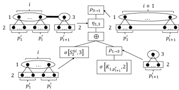
Figure 8: Expression tree for $S_{2}$. An ellipse is a clique and a rectangle is an independent set. An integer beside an ellipse or a rectangle is the label of the vertices in it. A bold line indicates that all the vertices in the endpoints are adjacent.

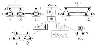
Figure 9: Expression tree for ${S_{2}^{I}}$.

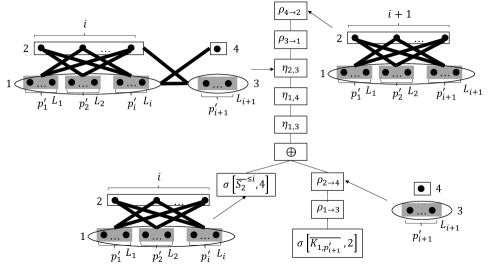
Figure 10: Expression tree for $\overline{S_{2}}$.

References

- [1] Borri, A., Calamoneri, T., Petreschi, R.: Recognition of unigraphs through superposition of graphs. J. Graph Algorithms Appl. 15(3), 323–343 (2011). https://doi.org/10.7155/jgaa.00229
- [2] Brandstädt, A., Le, V.B., Spinrad, J.P.: Graph Classes: A Survey. Society for Industrial and Applied Mathematics, Philadelphia, PA, USA (1999)
- [3] Brandstädt, A., Lozin, V.V.: On the linear structure and clique-width of bipartite permutation graphs. Ars Comb. 67 (2003)
- [4] Calamoneri, T., Petreschi, R.: The l(2, 1)-labeling of unigraphs. Discret. Appl. Math. 159(12), 1196–1206 (2011). https://doi.org/10.1016/j.dam.2011.04.015
- [5] Chvátal, V., Hammer, P.L.: Aggregation of inequalities in integer programming. In: Hammer, P., Johnson, E., Korte, B., Nemhauser, G. (eds.) Studies in Integer Programming, Annals of Discrete Mathematics, vol. 1, pp. 145–162. Elsevier (1977)
- [6] Corneil, D.G., Habib, M., Lanlignel, J., Reed, B.A., Rotics, U.: Polynomial-time recognition of clique-width 3 graphs. Discret. Appl. Math. 160(6), 834–865 (2012). https://doi.org/10.1016/j.dam.2011.03.020
- [7] Corneil, D.G., Rotics, U.: On the relationship between clique-width and treewidth. SIAM J. Comput. 34(4), 825–847 (2005). https://doi.org/10.1137/S0097539701385351
- [8] Courcelle, B., Engelfriet, J., Rozenberg, G.: Handle-rewriting hypergraph grammars. J. Comput. Syst. Sci. 46(2), 218–270 (1993). https://doi.org/10.1016/0022-0000(93)90004-G
- [9] Courcelle, B., Makowsky, J.A., Rotics, U.: Linear time solvable optimization problems on graphs of bounded clique-width. Theory Comput. Syst. 33(2), 125–150 (2000). https://doi.org/10.1007/s002249910009
- [10] Courcelle, B., Olariu, S.: Upper bounds to the clique width of graphs. Discret. Appl. Math. 101(1-3), 77–114 (2000). https://doi.org/10.1016/S0166-218X(99)00184-5
- [11] Fellows, M.R., Rosamond, F.A., Rotics, U., Szeider, S.: Clique-width is NP-complete. SIAM J. Discret. Math. 23(2), 909–939 (2009). https://doi.org/10.1137/070687256
- [12] Foldes, S., Hammer, P.: On a class of matroid-producing graphs. In: Colloq. Math. Soc. J. Bolyai (Combinatorics). vol. 18, pp. 331–352 (1978)
- [13] Golumbic, M.C., Rotics, U.: On the clique-width of some perfect graph classes. Int. J. Found. Comput. Sci. 11(3), 423–443 (2000). https://doi.org/10.1142/S0129054100000260
- [14] Hammer, P., Zverovich, I.: Splitoids. Graph Theory Notes N. Y. 46, 36–40
- [15] Heule, M., Szeider, S.: A SAT approach to clique-width. ACM Trans. Comput. Log. 16(3), 24:1–24:27 (2015). https://doi.org/10.1145/2736696
- [16] Johansson, O.: Clique-decomposition, NLC-decomposition, and modular decomposition - relationships and results for random graphs. Congressus Numerantium 132, 39–60 (1998), cited By 54
- [17] Johnson, R.H.: Simple separable graphs. Pacific J. Math. 56(1), 143–158 (1975)
- [18] Kaminski, M., Lozin, V.V., Milanic, M.: Recent developments on graphs of bounded clique-width. Discret. Appl. Math. 157(12), 2747–2761 (2009). https://doi.org/10.1016/j.dam.2008.08.022
- [19] Kleitman, D.J., Li, S.Y.: A note on unigraphic sequences. Studies in Applied Mathematics 54(4), 283–287 (1975)
- [20] Kobler, D., Rotics, U.: Edge dominating set and colorings on graphs with fixed clique-width. Discret. Appl. Math. 126(2-3), 197–221 (2003). https://doi.org/10.1016/S0166-218X(02)00198-1
- [21] Li, S.Y.R.: Graphic sequences with unique realization. J. Comb. Theory, Ser. B 19(1), 42–68 (1975)
- [22] Oum, S., Seymour, P.D.: Approximating clique-width and branch-widthssss. J. Comb. Theory, Ser. B 96(4), 514–528 (2006). https://doi.org/10.1016/j.jctb.2005.10.006
- [23] Peled, U.N.: Matroidal graphs. Discret. Math. 20, 263–286 (1977). https://doi.org/10.1016/0012-365X(77)90066-8
- [24] Rao, M.: MSOL partitioning problems on graphs of bounded treewidth and clique-width. Theor. Comput. Sci. 377(1-3), 260–267 (2007). https://doi.org/10.1016/j.tcs.2007.03.043
- [25] Tyshkevich, R.: Decomposition of graphical sequences and unigraphs. Discret. Math. 220(1-3), 201–238 (2000). https://doi.org/10.1016/S0012-365X(99)00381-7