Models with two right-handed neutrinos are able to accommodate solar and atmospheric neutrino oscillation observations as well as a mechanism for the baryon asymmetry of the universe. While economical in terms of the required new states beyond the Standard Model, given that there are three generations of the other leptons and quarks this raises the question concerning why only two right-handed neutrino states should exist. Here we develop from first principles a fundamental unification scheme based upon a direct generalisation and analysis of a simple proper time interval with a structure beyond that of local 4-dimensional spacetime and further augmenting that of models with extra spatial dimensions. This theory leads to properties of matter fields that resemble the Standard Model, with an intrinsic left-right asymmetry which is particularly marked for the neutrino sector. It will be shown how the theory can provide a foundation for the natural incorporation of two right-handed neutrinos and may in principle underlie firm predictions both in the neutrino sector and for other new physics beyond the Standard Model. While connecting with contemporary and future experiments the origins of the theory are motivated in a similar spirit as for the earliest unified field theories.

1 Introduction and Reviews

A salient feature of the history of physics is the progression in experimental and theoretical insights delving deeper into the structure of matter on ever smaller scales. While the regularity of chemical elements in the Periodic Table, as originally organised by Mendeleev in 1869, provided the first indirect hint of an inner structure for atoms, the familiar pattern of elementary particles established in the 1970s in the Standard Model encapsulates an order in the structure of matter at a further submicroscopic level. A central characteristic of this structure is the empirically uncovered distinctive symmetry properties of the elementary particle multiplets. Given the very fundamental level of these observations the modern-day quest to theoretically elucidate the underlying source of these symmetries of the Standard Model, in preference to positing them as ‘brute facts’ about the world, is particularly pressing.

This quest is analogous then, at a more elementary level, to the pursuit of an explanation for the Periodic Table that culminated in the discovery of the central atomic nucleus and the quantum mechanical properties of electron orbital states around one hundred years ago. While having something in common with the ‘unified field theories’ of that era, in this paper we describe a new theory based upon a generalisation of proper time which has the potential to naturally incorporate not only the Standard Model but also the phenomenology of physics beyond, including that of the neutrino sector. The core arguments for this analysis are summarised in [1] and will be elaborated along with further observations in this paper as outlined below.

In the first subsection to follow we review the empirically established properties of neutrinos and several of the models stimulated by these results. We then present an historical survey of early unified field theories in subsection 1.2 which will lead to a probing of the motivation for extra spatial dimensions and the application of a further generalisation for a proper time interval in section 2. (This paper can be read beginning with section 2, with section 1 for reference). In section 3 the greater suitability of this generalisation in directly accounting for features of the Standard Model will be explained, further justifying the new approach. The manner in which this theory might naturally provide a foundation for models with two right-handed neutrinos will be described in subsection 4.1, with broader connections with new physics beyond the Standard Model and further possible tests discussed in subsection 4.2. We return to the interpretation of theory and its relation to special and general relativity and connection with early unified field theories in subsection 5.1, with the underlying simplicity of the theory evaluated further in subsection 5.2. In section 6 we conclude with emphasis on the opportunities for the further development of this fundamental theory. The main goals of this paper are summarised here:

• A main theme of the paper is to emphasise the simplicity of this theory based on a generalisation of proper time, arguing that a unifying basis for fundamental physics can be encapsulated correspondingly in ‘one simple equation’.

• We describe how the theory can be seen as a natural progression from special and general relativity, while also being complementary to the latter, and is related to the early conceptions of a unified field theory.

• While reviewing the links with the Standard Model here we focus on possible connections with the further esoteric properties of physics beyond, in particular establishing a link with models incorporating two right-handed neutrinos.

The theory, originating from considerations of the first bullet point above, will be shown to provide a connection between the old and the new, from the second and the third bullet points respectively, by demonstrating the relevance of the theory for contemporary particle physics and cosmology. With this aim in mind we begin by reviewing the current status of the neutrino sector.

1.1 Neutrino Physics

The striking progress in the empirical understanding of neutrino physics in recent decades has centred upon the compelling observations of oscillations between the left-handed neutrino states. These can be described assuming three-flavour neutrino mixing parametrised by the $3\times 3$ complex unitary Pontecorvo-Maki-Nakagawa-Sakata, or PMNS, matrix (see for example [2] sections 14.1 and 14.2, [3] section 2.1) which expresses the non-trivial relation between the three left-handed neutrino flavour eigenstates $\nu_{e}$, $\nu_{\mu}$ and $\nu_{\tau}$ and three mass eigenstates $\nu_{1}$, $\nu_{2}$ and $\nu_{3}$ with respective masses $m_{1}$, $m_{2}$ and $m_{3}$.

This structure accommodates both the ‘solar neutrino’ oscillations, which are predominantly described by the mixing probability $P(\nu_{e}\to\nu_{\mu})$, as confirmed by nuclear reactor experiments, via a mixing angle $\theta_{\mathrm{sol}}=\theta_{12}\simeq 33.6^{\circ}$ and mass difference $\Delta m^{2}_{\mathrm{sol}}=\Delta m^{2}_{21}:=m_{2}^{2}-m_{1}^{2}\simeq 7.5\times 10^{-5}\,\mbox{eV}^{2}$, as well as the ‘atmospheric neutrino’ oscillations which can be assumed to be almost completely due to the mixing probability $P(\nu_{\mu}\to\nu_{\tau})$, as confirmed by accelerator experiments, via a mixing angle $\theta_{\mathrm{atm}}=\theta_{23}\simeq 40$–$50^{\circ}$ and mass difference $\Delta m^{2}_{\mathrm{atm}}=\Delta m^{2}_{32}:=m_{3}^{2}-m_{2}^{2}\simeq 2.5\times 10^{-3}\,\mbox{eV}^{2}$ (with all data in this subsection obtained from [2] unless stated otherwise). The third mixing angle has also been determined as $\theta_{13}\simeq 8.4^{\circ}$, principally from the disappearance of $\bar{\nu}_{e}$ produced in nuclear fission reactors ([2] section 14.12), while an estimate of the phase of the PMNS matrix $\delta_{C\!P}\simeq\frac{3\pi}{2}$ has been obtained from long baseline accelerator $\stackrel{{\scriptstyle\raisebox{-2.0pt}[0.0pt][0.0pt]{\mbox{{\tiny\>\!({\bf--})}}}}}{{\raisebox{0.0pt}[0.0pt][0.0pt]{\mbox{$\nu$}}}}_{\!\!\mu}\to\stackrel{{\scriptstyle\raisebox{-2.0pt}[0.0pt][0.0pt]{\mbox{{\tiny\>\!({\bf--})}}}}}{{\raisebox{0.0pt}[0.0pt][0.0pt]{\mbox{$\nu$}}}}_{\!\!e}$ appearance experiments ([2] section 14.13).

The third mass difference is determined from the definitions by the other two with $\Delta m_{31}^{2}=\Delta m_{32}^{2}-\Delta m_{21}^{2}$, and with $\Delta m_{31}^{2}\simeq\Delta m_{32}^{2}$ since $\Delta m_{21}^{2}$ is somewhat smaller than $\Delta m_{32}^{2}$. There is however no existing constraint on the sign of $\Delta m_{32}^{2}$, that is whether $m_{3}$ is greater or less than $m_{2}$ (and $m_{1}$) – termed the ‘normal’ or ‘inverted’ hierarchy respectively. The neutrino oscillation data also does not determine the absolute mass scale.

The electron neutrino mass $m_{\nu_{e}}$ can be defined by $m_{\nu_{e}}^{2}=\sum_{i=1}^{3}|U_{ei}|^{2}m_{i}^{2}$, where $U_{ei}$ are elements of the top row of the PMNS matrix. The measured parameters above, given that the lightest neutrino mass state has mass $m_{\mathrm{min}}\geq 0\,\mbox{eV}$, set lower bounds of $m_{\nu_{e}}>0.01\,\mbox{eV}$ for the normal hierarchy and $m_{\nu_{e}}>0.05\,\mbox{eV}$ for the inverted hierarchy. A direct upper limit on the electron neutrino mass is set by tritium $\beta$-decay experiments with $m_{\nu_{e}}<2.0\,\mbox{eV}$, with future experiments aiming to bring this limit down to $m_{\nu_{e}}<0.2\,\mbox{eV}$ [4].

By comparison for $m_{\mathrm{min}}=0\,\mbox{eV}$ the simple sum of the three neutrino masses $m_{\mathrm{tot}}=\sum_{i=1}^{3}m_{i}$ would be $m_{\mathrm{tot}}=0.06\,\mbox{eV}$ or $m_{\mathrm{tot}}=0.10\,\mbox{eV}$ for the normal or inverted mass hierarchy respectively (see also [3] section 2.1). The constraints from cosmological observations, although dependent upon the $\Lambda$CDM cosmological model (with $\Lambda$ the cosmological constant and CDM cold dark matter), imply $m_{\mathrm{tot}}<0.12\,\mbox{eV}$ at the 95% confidence level [5], already putting pressure on the inverted hierarchy. Future prospects for the three left-handed neutrinos within the $\Lambda$CDM model are for the lowest possible value of $m_{\mathrm{tot}}=0.06\,\mbox{eV}$ to be detectable at the 3–4$\sigma$ level in the coming years ([2] sections 25.4 and 64).

While the existing data cannot distinguish between whether neutrinos are Dirac or Majorana fermions, any observation of neutrinoless double-$\beta$ decay would indicate the Majorana type (that is, with such a neutrino identical to its own antiparticle state). If such experiments were to determine a non-zero value for the appropriately defined effective Majorana mass $m_{\beta\beta}$ for this process with $m_{\beta\beta}\lesssim 0.01\,\mbox{eV}$, an order of magnitude beyond the current sensitivity, then the inverted hierarchy could be ruled out ([6], [2] section 62, [3] section 3.3). Such a measurement with $m_{\beta\beta}\gtrsim 0.005\,\mbox{eV}$ would also indicate that $m_{\mathrm{min}}>0\,\mbox{eV}$ ([2] figure 62.1, [3] figure 5). Similarly, there remains the possibility for a positive observation of neutrinoless double-$\beta$ decay with $m_{\beta\beta}\gtrsim 0.06\,\mbox{eV}$ also implying a value for $m_{\mathrm{min}}>0\,\mbox{eV}$, although in this case in a range seemingly in tension with the above current cosmological bound.

The observation of neutrino oscillations is generally considered to imply the existence of right-handed neutrinos $\nu_{R}$ which are ‘sterile’, that is they transform trivially under the Standard Model gauge group $\mbox{SU}(3)_{c}\times\mbox{SU}(2)_{L}\times\mbox{U}(1)_{Y}$, accounting for the difficulty of their direct detection (unlike the familiar ‘active’ left-handed states $\nu_{L}$ that undergo weak interactions). These right-handed states can be utilised to introduce light masses for the active neutrinos by extending the Standard Model Lagrangian with further Dirac mass terms. Such terms are similar to those for the charged leptons and quarks but with unnaturally small Yukawa couplings to the Higgs field, by around a factor of $10^{-12}$ relative to that of the top quark and even by a factor of $10^{-6}$ or less relative to that of the electron in the same weak doublet as the electron neutrino. However, owing to their trivial gauge transformation properties, Majorana mass terms can also be added for the right-handed neutrinos which, if sufficiently heavy, can generate the light active neutrino masses via a ‘seesaw’ mechanism ([3] section 2 and references therein). For either of the above cases, since each $\nu_{R}$ state can only generate one $\nu_{L}$ mass, at least two right-handed neutrinos are required to account for at least two finite active neutrino masses as implied by the established measurements of $\Delta m_{21}$ and $\Delta m_{32}$, unless there is a different source for the $\nu_{L}$ masses.

In the absence of a theoretical argument to the contrary a natural expectation might be for all three active neutrinos to be massive, via the introduction of three right-handed neutrino states, matching the three generation structure of the other leptons and quarks. This is the case for the ‘Neutrino Minimal Standard Model’, or $\nu$MSM ([7, 8], [3] section 7), proposed as a simple economical extension from the Standard Model (for which all three $\nu_{L}$ states are massless and there are no $\nu_{R}$ states). In the $\nu$MSM there are two $\nu_{R}$ states with nearly degenerate masses in the range from $\sim\!\!1\,\mbox{GeV}$ to the electroweak scale which account for active neutrino masses via the seesaw mechanism consistent with the well-established neutrino oscillation data. At the epoch of the Big Bang $C\!P$-violating oscillations of these two sterile neutrinos during their thermal production can also in principle generate the baryon asymmetry of the universe.

Compelling empirical evidence for the mass scale of right-handed neutrinos may be even harder to establish than for the active left-handed states. However the lower part of the preferred mass range of $1\!\!\sim\!\!100\,\mbox{GeV}$ for two of the three right-handed neutrinos in the $\nu$MSM could be accessible to direct searches for $\nu_{R}$ states through mixing with active neutrino states in laboratory experiments ([3] section 3.4, [9]). Such mixing is required to generate the active $\nu_{L}$ masses via the seesaw mechanism. Further, much lighter right-handed neutrinos can also play a significant role in cosmology [10].

In particular, sterile right-handed neutrinos, which apart from the above mixing effects could only be observable through gravitational interactions, can be considered a natural candidate for dark matter [11]. However the required Yukawa couplings for this application are very different to those associated with neutrino oscillations. In the case of the $\nu$MSM the third $\nu_{R}$ state, with a mass of a few keV, acts as a warm dark matter candidate but with a Yukawa coupling too small to make a significant contribution to the active neutrino masses, hence leaving the lightest active neutrino practically massless. More generally, for scenarios with three $\nu_{R}$ states there is no intrinsic limit on the mass of the lightest $\nu_{L}$ mass state.

Neutrino models are further stretched if required to accommodate the empirical hints for anomalous observations in $\stackrel{{\scriptstyle\raisebox{-2.0pt}[0.0pt][0.0pt]{\mbox{{\tiny\>\!({\bf--})}}}}}{{\raisebox{0.0pt}[0.0pt][0.0pt]{\mbox{$\nu$}}}}_{\!\!\mu}\to\stackrel{{\scriptstyle\raisebox{-2.0pt}[0.0pt][0.0pt]{\mbox{{\tiny\>\!({\bf--})}}}}}{{\raisebox{0.0pt}[0.0pt][0.0pt]{\mbox{$\nu$}}}}_{\!\!e}$ oscillations, which imply a mass difference of $\Delta m^{2}\sim\!1\,\mbox{eV}^{2}$, as well as the anomalies observed in reactor and gallium experiments. Further neutrino states or other new features are needed to provide a phenomenologically complete description of all neutrino particle physics data (see for example [12]).

On the other hand the compelling neutrino oscillation observations can be accounted for by models with only two right-handed neutrinos, which can also accommodate a source of the baryon asymmetry (see for example [13, 14, 15, 16]). For these models, which imply that $m_{\mathrm{min}}=0\,\mbox{eV}$ for the left-handed neutrinos, the two right-handed neutrinos are typically very massive in the range from $\sim\!\!10^{10}\,$GeV up to the GUT scale. In this case a possible source of the matter-antimatter asymmetry derives through a leptogenesis scenario via heavy right-handed neutrino decays in the very early universe (see also [17, 18]). The indications that the PMNS phase $\delta_{C\!P}$ may be relatively large suggests that $C\!P$-violating effects in the oscillations of light active neutrinos may be significant, and can be linked via the neutrino mass matrices in specific seesaw models with the $C\!P$-violating phase in the heavy sterile neutrino sector that drives the baryon asymmetry via leptogenesis (see for example [13], [18] section 8, [19]). While models with two $\nu_{R}$ states might hence account for active neutrino oscillations and the baryon asymmetry, similarly as for the $\nu$MSM, in lacking a third $\nu_{R}$ state an alternative candidate for dark matter will be required.

In summary, based only upon well-established observations in the neutrino sector the main questions to be addressed concern the absolute value and spectrum of the active neutrino masses, resolving the sign of $\Delta m_{32}^{2}$, the number and masses of sterile neutrinos, and whether neutrinos are Dirac or Majorana particles. Further questions concern the PMNS matrix: including the proximity of the value of $\theta_{23}$ to maximal $45^{\circ}$ mixing, the need for a more precise evaluation of $\delta_{C\!P}$, and regarding the relation of the neutrino mixing matrix to the very different CKM mixing matrix in the quark sector.

While it is always possible in principle to model a wide range of neutrino phenomena, by extending the Standard Model Lagrangian, a more fundamental explanation of the origin of these empirical observations, providing a deeper understanding of the neutrino flavour structure and mass generation mechanism, would of course be desired. Ideally such an explanation would take the form of a theory that also accounts for the properties of the Standard Model itself, and which might be empirically tested in neutrino experiments, in the particle physics laboratory more generally or through cosmological observations. In this paper we propose such a fundamental theory. The theory may provide in particular a possible basis for models with two right-handed neutrinos in a unified structure consistently alongside three generations of the other leptons and quarks, as will be explained in subsection 4.1. While connecting with these contemporary phenomenological issues, as described further in subsection 4.2, the underlying motivation for the theory is related to that for the earliest unified field theories; we hence next review this background in the following subsection.

1.2 Unified Field Theories

While the field concept as employed with great success for Maxwell’s equations [20] had very much influenced the conception of Einstein’s theory of general relativity [21] half a century later, after 1915 it was natural seek a unified field theory that would generalise the theory of gravity to incorporate electromagnetism, rather than the other way around. The reason for this is perhaps that while the gravitational field equations are more complicated than those for electromagnetism the underlying motivation envisaged for Einstein’s theory can be considered somewhat simpler. As a particularly elegant aspect of general relativity the assumption of an extended globally flat 4-dimensional Minkowski spacetime is dropped, with special relativity holding for all non-gravitational physics strictly only in the limit of infinitesimally small inertial reference frames by the equivalence principle ([22] chapter 9). Within such a local reference frame with local coordinates $\{x^{a}\}$ an infinitesimal proper time interval $\delta s$ can be expressed, in a form invariant under local $\mbox{SO}^{+}(1,3)$ Lorentz transformations between such frames, as:

$$(\delta s)^{2}=(\delta x^{0})^{2}-(\delta x^{1})^{2}-(\delta x^{2})^{2}-(\delta x^{3})^{2}\;=\;\eta_{ab}\delta x^{a}\delta x^{b}$$ (1)

with the Lorentz metric $\eta=\mbox{diag}(+1,-1,-1,-1)$ and $a,b=0,1,2,3$ (the summation convention for repeated indices is assumed throughout this paper).

In special relativity there exist sets of global coordinates $(x^{0},x^{1},x^{2},x^{3})$ in which equation 1 holds for arbitrary finite spacetime intervals anywhere in the Minkowski spacetime, leaving the corresponding finite proper time interval $\Delta s$ invariant under global Lorentz transformations between such reference frames. This framework of special relativity was largely motivated through compatibility with Maxwell’s equations, with the laws of electrodynamics taking the same form in any of these global inertial reference frames [23].

In general relativity there are no such global coordinates and inertial frames, except in the flat spacetime limit. Instead general coordinates $\{x^{\mu}\}$, with $\mu,\nu=0,1,2,3$, must be defined on the global scale, with respect to which a local infinitesimal proper time interval can be expressed in a manner invariant under general coordinate transformations as:

$$(\delta s)^{2}\;=\;g_{\mu\nu}(x)\delta x^{\mu}\delta x^{\nu}$$ (2)

which only locally reduces to equation 1 in suitable local coordinates. The force of gravity is not present in such a local inertial reference frame but rather can be ascribed globally to the metric field $g_{\mu\nu}(x)$ which describes the curved geometry of the extended spacetime. Through a mutual dynamical interplay the spacetime geometry described by $g_{\mu\nu}(x)$ is related to the distribution of matter through Einstein’s field equation (as will be discussed in subsection 5.1 for equation 105), with test particles postulated to propagate through spacetime along geodesic trajectories. Einstein’s theory of gravity, expressed directly in terms of the more general and flexible structure of a curved spacetime, surpassed that of Newton in accurately accounting for gravitational observations such as the orbit of the planet Mercury. While Newton’s law of universal gravitation strictly concerned mathematical relations, and was not based on any hypothesis regarding the cause of the force of gravity acting at a distance across space, for Einstein the curvature of spacetime also succeeded in furnishing an explanation of gravitational phenomena on relaxing the assumption of spacetime flatness.

On the other hand for Maxwell’s electromagnetism, initially formulated in a Newtonian background of absolute space and time, 3-component electric $E$ and magnetic $B$ fields were first added, conceived of as mechanical states of an underlying ‘ethereal medium’ filling all of space ([20] part I, see also [22] section 6(a) and [24] section 12(a) part 1); with Maxwell’s equations constructed on the basis of empirical observations, as Newton’s law of gravity had been in the same background arena. After 1905, with the theory of electromagnetism readily compatible with special relativity, Maxwell’s equations could be expressed more succinctly in a Lorentz covariant form in terms of the antisymmetric electromagnetic field strength tensor $F_{\mu\nu}(\mbox{\boldmath$E$},\mbox{\boldmath$B$})$, and after 1915 could be accommodated within the curved spacetime of general relativity via the equivalence principle. However, it was natural to enquire whether a further generalisation from general relativity might itself provide an explanation of electromagnetism (which alongside gravity was then the only other fundamental force known) on relaxing further assumptions regarding the 4-dimensional spacetime metric geometry.

The first proposal for such a unified field theory was made in 1918 by Weyl ([25], [26] chapter IV section 35, [27] chapters 1–3) on dropping the assumption that the length of a 4-vector, determined by the metric $g_{\mu\nu}(x)$ of equation 2, should be path-independent when ‘parallel transported’ in spacetime, an invariance which could be interpreted as a residual of rigid Euclidean geometry still remaining in general relativity. Hence, similarly as a 4-vector direction is propagated in a path-dependent manner through a curved spacetime via a linear connection $\Gamma^{\rho}_{\phantom{\rho}\mu\nu}(x)$, a unique function of the first derivatives of $g_{\mu\nu}(x)$ in general relativity, Weyl introduced a vector field $A_{\mu}(x)$ to induce path-dependent changes to 4-vector magnitudes – with the metric $\bar{g}_{\mu\nu}(x)$ employed in forming inner products defined by the scaling:

$$\bar{g}_{\mu\nu}(x)=\lambda\,g_{\mu\nu}(x)\qquad\mbox{with}\qquad\lambda=e^{\int_{x_{1}}^{x_{2}}A_{\mu}(x)dx^{\mu}}$$ (3)

The length of a 4-vector is path-independent under parallel transport between any two spacetime points $x_{1}$ and $x_{2}$ only when the scale factor $\lambda$ is integrable. This is the case if the new connection field $A_{\mu}(x)$ can be expressed as the gradient of a continuous function $\chi(x)$, that is $A_{\mu}(x)=\partial_{\mu}\chi(x)$, which in turn implies that the quantity defined by $F_{\mu\nu}(x)=\partial_{\mu}A_{\nu}(x)-\partial_{\nu}A_{\mu}(x)$ vanishes. In the general case the field $F_{\mu\nu}(x)$ was identified with the electromagnetic field strength tensor and $A_{\mu}(x)$ with the corresponding vector potential, within normalisation factors, similarly as the Riemann curvature tensor together with $\Gamma^{\rho}_{\phantom{\rho}\mu\nu}(x)$ and $g_{\mu\nu}(x)$ are associated with gravity in general relativity. In this manner Weyl inferred that on the 4-dimensional spacetime manifold ‘all physical field-phenomena are expressions of the metrics of the world’ ([26] chapter IV section 35). The theory hence demonstrated that electromagnetism could in principle be accorded such a geometrical significance. However, since scaling lengths via $\lambda$ in equation 3 implies scaling time intervals also in equation 2 Einstein immediately noted a fatal flaw of the theory – the sharp lines of atomic spectra observed in the laboratory are not dependent upon the history of individual atoms.

Weyl’s theory did however provide the first step towards non-Riemannian connections and gauge theories, with the term ‘gauge’ retained from the length scaling factor in equation 3. In fact both $F_{\mu\nu}(x)$ and the ‘Action’ defined for the theory are ‘gauge-invariant’ under arbitrary re-calibrations, that is under local changes of the adopted metric scale. Progress was achieved by 1929 on introducing a factor of $i=\sqrt{-1}$ in the exponent in equation 3 and reinterpreting $\lambda$ as a phase factor to be applied instead to a complex wavefunction $\Psi(x)$ in the then recently invented quantum mechanics ([28], [29] chapter II section 12, [27] chapters 4–5). Correspondingly in [28] Weyl concludes with the assessment that ‘electromagnetism is an accompanying phenomenon of the material wave-field and not of gravitation’. Hence with the phase factor taking values in the symmetry group $\mbox{U}(1)$ electromagnetism could be successfully described as a stand-alone $\mbox{U}(1)$ gauge theory with a gauge field $A_{\mu}(x)$, rather than as a geometric augmentation to general relativity. During the 1950s–1970s such gauge theories, with field interactions considered a consequence of the gauge-invariance of the equations, were developed and generalised beyond the $\mbox{U}(1)$ gauge symmetry of electromagnetism to non-Abelian gauge symmetries, ultimately incorporating electroweak and strong interactions also within the framework of the ‘gauge principle’, essentially detached from consideration of the geometry of external 4-dimensional spacetime – which could be taken as the flat background of special relativity to a very good approximation in a laboratory setting.

The properties and representations of gauge symmetry groups are central to the modern-day structure of the Standard Model and unification schemes. It is well known for example that the branching patterns for the smaller non-trivial representations of Lie groups such as SU(5), SO(10), $\mbox{E}_{6}$ and $\mbox{E}_{7}$ on extracting the Standard Model subgroup $\mbox{SU}(3)_{c}\times\mbox{SU}(2)_{L}\times\mbox{U}(1)_{Y}$ bear some resemblance to the gauge multiplet structure of leptons and quarks ([30], [31] section 13, [32] and [33] respectively) as the basis for a Grand Unified Theory (GUT). While the earlier unified field theories were based on generalisations of general relativity, for GUT models the focus is on particle physics with gravity being neglected and deferred for later consideration. However, in the case of the Lie group $\mbox{E}_{8}$ a symmetry breaking structure can be correlated with a full three generations of leptons and quarks incorporating also transformations under the external local spacetime Lorentz symmetry alongside the Standard Model gauge group [34]. Nevertheless for each of the above Lie group structures the match with the symmetry properties of the Standard Model is incomplete and significant problems remain. Further, while the three largest exceptional Lie groups $\mbox{E}_{6}$, $\mbox{E}_{7}$ and $\mbox{E}_{8}$ are of particular interest, owing to the high degree of symmetry they describe and the uniqueness of these mathematical structures, the nature of a clear underlying conceptual origin, whether geometric or otherwise, to motivate the application of these groups in particle physics remains an open question.

Despite his rejection of Weyl’s theory Einstein himself sought a unified field theory for gravity and electromagnetism based on generalisations of general relativity. From 1925–1955, throughout the last 30 years of his life, Einstein worked on generalisations of 4-dimensional Riemannian geometry based in particular on dropping the assumption that the metric tensor ${g}_{\mu\nu}(x)$ and/or the linear connection ${\Gamma}^{\rho}_{\phantom{\rho}\mu\nu}(x)$ should be symmetric in the $\mu,\nu$ indices ([22] section 17(e)). The most direct attempt introduced a nonsymmetric fundamental tensor $\tilde{g}_{\mu\nu}(x)$ with a full 16 real components which was proposed to decompose into symmetric $g_{\mu\nu}(x)$ and antisymmetric $\acute{g}_{\mu\nu}(x)$ parts as:

$$\tilde{g}_{\mu\nu}(x)\;=\;g_{\mu\nu}(x)\;[\mbox{gravitational field}]\;+\;\acute{g}_{\mu\nu}(x)\;[\mbox{electromagnetic field}]$$ (4)

For this scheme $g_{\mu\nu}(x)$ was retained as the original gravitational metric field while $\acute{g}_{\mu\nu}(x)$ was identified with the electromagnetic field strength tensor $F_{\mu\nu}(x)$, within a normalisation constant. Other attempts involved associating the electromagnetic vector potential $A_{\mu}(x)$ with components of a nonsymmetric linear connection. (In an independent application the study of linear connections with an antisymmetric part had been initiated by Cartan in 1922 in the geometric context of general relativity with finite torsion, later known as Einstein-Cartan theories). While originally motivated by simplicity Einstein’s unified field theory attempts became increasingly elaborate, lacking the conceptual elegance of general relativity, and none of them led to the free Maxwell equations even in the weak-field approximation, nor was there any prospect of incorporating nuclear forces into these schemes. During the same period, from around 1925, the mainstream physics community was also more focussed upon the developments of quantum theory, with the unification proposals of Einstein seemingly attracting more attention from The New York Times ([22] section 17(e)). However, while our understanding of fundamental physics has continued to be dominated by quantum theory, the general spirit and motivation for Einstein’s attempts at a unified field theory remains enlightening when transplanted into the context of the present-day quest for unification, as will be discussed in subsection 5.1.

Einstein had also been initially enthusiastic about the potential of Kaluza-Klein theory as also introduced in the 1920s ([35, 36], [22] section 17(c)), upon which he worked intermittently himself over a number of years ([22] sections 17(c,e)). In this approach to a unified field theory the assumption that spacetime should be limited to the familiar 4-dimensional arena of general relativity was dropped. With 4-dimensional spacetime augmented by an extra spatial dimension a $5\times 5$ metric $\hat{g}(x)$ could be defined on the extended spacetime subsuming the original $4\times 4$ metric ${g}(x)$ of equation 2. In principle the four components of the electromagnetic vector potential $A(x)$ could then be accommodated inside the extended 5-dimensional metric:

$$\left[\begin{array}[]{c}\\ \vspace{2pt}\hfil\\ \end{array}\;\;\,\hat{g}\;\;\,\begin{array}[]{c}\\ \vspace{2pt}\hfil\\ \end{array}\right]_{5\times 5}=\;\left[\!\!\!\begin{array}[]{cc}\left[\begin{array}[]{c}\vspace{1pt}\hfil\\ \end{array}g\begin{array}[]{c}\vspace{1pt}\hfil\\ \end{array}\right]&\!\!\!\!\!\!\left[\begin{array}[]{c}\vspace{1pt}\hfil\\ \end{array}\!\!\!\!\!\!A\!\!\!\!\!\!\begin{array}[]{c}\vspace{1pt}\hfil\\ \end{array}\right]\!\!\!\vspace{-2pt}\\ \left[\;\;\,A^{\!\mbox{\tiny{\it T}}}\;\;\,\right]&\!\!\!\!\!\!\phi\!\!\!\vspace{-2pt}\end{array}\right]$$ (5)

where the further new component $\phi(x)$, alongside the original metric $g(x)$ of general relativity, lacked any clear physical significance. Certain components of the 5-dimensional Levi-Civita linear connection $\hat{\Gamma}(x)$ could then be identified with the electromagnetic field strength $F_{\mu\nu}(x)=\partial_{\mu}A_{\nu}(x)-\partial_{\nu}A_{\mu}(x)$ as a function of the components $A_{\mu}(x)$ in equation 5 in the appropriate way, on taking the field values to be independent of the fifth dimension. Maxwell’s source-free equations for the electromagnetic field and the equation of motion for a charged body in an electromagnetic field could be obtained under suitable assumptions for the extraction of 4-dimensional physics from the embedding in the 5-dimensional spacetime framework. However, while hence providing an element of formal geometric unification with general relativity, no predictive power or new phenomena could be determined and the question of the very different properties required for the fifth dimension remained.

In the case of equation 3 with a geometric scale factor $\lambda$ and that of equation 4 with a nonsymmetric metric $\tilde{g}_{\mu\nu}$ no further natural generalisation is possible, however for the case of equation 5 an arbitrary number of further extra spatial dimensions could in principle be considered. Indeed, despite the lack of empirical support, this third means of augmenting the 4-dimensional spacetime structure has led in recent decades to a large number of unification models based upon various approaches to extra spatial dimensions, motivated in part by the elegance and unity of the Kaluza-Klein idea.

The realisation that the geometry of such augmented spacetimes could be adapted to incorporate the internal symmetries of non-Abelian gauge theory over 4-dimensional spacetime, with a close relation between gauge and coordinate transformations described explicitly on a ‘fibre bundle’ manifold, had revived interest in this approach to unification by the 1970s. (See for example [37], the mathematics of fibre bundles had been developed since 1935 for the field of topology in differential geometry [38] independently of any application in physics). This framework ‘combined gravitation with gauge theory in the context of a unified geometric theory in the bundle space’ ([37] section 9) by employing an extended higher-dimensional metric defined on the full space. In this manner gauge theory, which had parted company from a geometric context in the 1920s as described above following equation 3, was placed in the setting of a higher-dimensional spacetime arena, and in particular reattached to the geometry of an external 4-dimensional spacetime base manifold, in a unifying physical framework that might in principle reach beyond gravitation and electromagnetism alone.

While the earliest attempts at a unified field theory may have been premature, given the hindsight of the subsequent century of accumulated knowledge in particle physics, the quest since the 1970s to accommodate the rich properties of the Standard Model, or even a Grand Unified Theory, within the unifying framework of geometric structures deriving from extra spatial dimensions over 4-dimensional spacetime continues, as will be discussed in the next subsection. The search now includes the need not only to account for the Standard Model but also new physics, such as that of the neutrino sector reviewed in the previous subsection. In this paper we shall motivate and build a new unified theory from first principles with the potential to accommodate both the physics of the Standard Model and that beyond, including the possible feature of incorporating two, and only two, right-handed neutrinos alongside three generations of the other leptons and quarks. We begin by reassessing the motivation for employing extra spatial dimensions in the following section.

2 Generalised Proper Time

2.1 Extra Spatial Dimensions and the Standard Model

Rather than considering generalisations of the global metric $g_{\mu\nu}(x)$ of equation 2 on an extended higher-dimensional spacetime manifold here we focus upon the local metric $\eta_{ab}$ of equation 1 associated with a local inertial reference frame. At this most elementary level of purely local structure theories with extra spatial dimensions extend the metric geometry of 4-dimensional spacetime, with local coordinates $(x^{0},x^{1},x^{2},x^{3})$, augmenting the quadratic expression for the proper time interval $\delta s$ of equation 1 to the $n$-dimensional form:

$$(\delta s)^{2}=(\delta x^{0})^{2}-(\delta x^{1})^{2}-(\delta x^{2})^{2}-(\delta x^{3})^{2}\,-\,(\delta x^{4})^{2}\ldots\ldots-(\delta x^{n-1})^{2}=\hat{\eta}_{ab}\delta x^{a}\delta x^{b}\;$$ (6)

where $(x^{4},\ldots,x^{n-1})$ are $(n-4)$ extra dimensions, $\hat{\eta}=\mbox{diag}(+1,-1,\ldots,-1)$ is the extended local Lorentz metric and $a,b=0,\ldots,(n-1)$. The additional components $(x^{4},\ldots,x^{n-1})$ are considered extra ‘spatial’ dimensions owing to the quadratic structure and the minus signs in equation 6, sharing these properties with the three original spatial dimensions given the Lorentz metric signature convention of equation 1. On dividing both sides by $(\delta s)^{2}$ and defining the components $v^{a}=\frac{\delta x^{a}}{\delta s}$ on taking the limit $\delta s\to 0$ the above expression can be written as:

$$|\mbox{\boldmath$v$}_{n}|^{2}:=\;\!(v^{0})^{2}-(v^{1})^{2}-(v^{2})^{2}-(v^{3})^{2}\,-\,(v^{4})^{2}\ldots\ldots-(v^{n-1})^{2}\;\!=\,\hat{\eta}_{ab}v^{a}v^{b}\,=\,1$$ (7)

in terms of the components of the ‘$n$-velocity’ vector $\mbox{\boldmath$v$}_{n}=(v^{0},\ldots,v^{n-1})\in{\mathbb{R}}^{n}$. The quantities $\delta s$ and $|\mbox{\boldmath$v$}_{n}|$ in equations 6 and 7 respectively are invariant under $\mbox{SO}^{+}(1,n-1)$ transformations applied to these $n$-component expressions.

The simplest and most direct means of constructing a physical theory based on this structure is to assume the identification of the four components $(x^{0},x^{1},x^{2},x^{3})$ in equation 6 with a set of local coordinates on an external spacetime $M_{4}$, without necessarily specifying a mechanism for distinguishing this extended manifold itself in four, and only four, preferred dimensions. The first four components $\mbox{\boldmath$v$}_{4}=(v^{0},v^{1},v^{2},v^{3})$ of equation 7 are correspondingly projected onto the local tangent space of the extended 4-dimensional spacetime, with $\mbox{\boldmath$v$}_{4}\in\mbox{\it TM}_{4}$, upon which a preferred local external $\mbox{SO}^{+}(1,3)\subset\mbox{SO}^{+}(1,n-1)$ symmetry acts. This breaks the full $n$-dimensional $\mbox{SO}^{+}(1,n-1)$ Lorentz symmetry of equation 7 and on taking the residual components of that equation to form the basis for ‘matter fields’ in the extended spacetime we directly deduce the following symmetry breaking structure:

$$\mbox{SO}^{+}(1,n-1) \to \mbox{SO}^{+}(1,3)\;\times\;\mbox{SO}(n-4)\quad\;\!\mbox{: external $\times$ internal$\;\;$}$$ (8)

$$\mbox{\boldmath$v$}_{4}\in{\mathbb{R}}^{4}\>\, : \mbox{\it TM}_{4}\;\;\;\;$$ 4-vectorinvariant: tangent vector in

$$\raisebox{0.0pt}[0.0pt][0.0pt]{ {\raisebox{7.3194pt}{$\!\!\mbox{\boldmath$v$}_{n}\in{\mathbb{R}}^{n}\!\to\!\left\{\!\begin{array}[]{c}\\ \vspace{-12pt}\hfil\end{array}\right.\!\!\!\!\!\!$}} }\underline{\mbox{\boldmath$v$}}_{n-4}\in{\mathbb{R}}^{n-4}\!\!\!\! : \;\>\,\mbox{scalar}\qquad\;\!\!\!(n-4)\mbox{-vector}\quad\!\!\!\mbox{: matter field over $M_{4}$}$$ (11)

This direct generalisation from the structure of a strictly 4-dimensional proper time interval of equation 1 is depicted in figure 1.

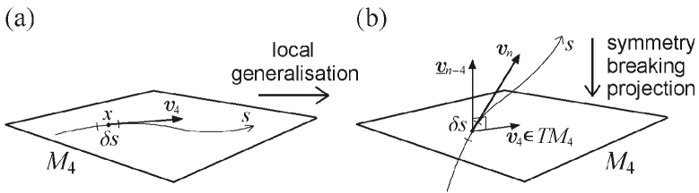
Figure 1: (a) A 4-vector field $\mbox{\boldmath$v$}_{4}(x)$ can be constructed from locally Lorentz invariant proper time intervals $\delta s$ at each point $x\in M_{4}$ and (b) augmented for time $s$ propagating through a higher-dimensional spacetime, with the corresponding local values of $\mbox{\boldmath$v$}_{n}(x)$ projected onto the external 4-dimensional spacetime $M_{4}$ here represented by a plane.

We note that although the projection takes place locally on the external manifold $M_{4}$ the action on $\underline{\mbox{\boldmath$v$}}_{n-4}(x)$ of the full internal symmetry $G=\mbox{SO}(n-4)$ implies the incorporation of this complete gauge group manifold in a ‘trivial principal fibre bundle’ structure $P\equiv M_{4}\times G$, with ‘vertical’ fibres $G$ attached over each point of the ‘base space’ $M_{4}$ of figure 1(b). (The case for $n=10$ in equation 8–11 is depicted in [39] figure 1(b) while the relation of this construction to the geometry of non-Abelian Kaluza-Klein theories is described in [40]). However in this simple picture the matter field $\underline{\mbox{\boldmath$v$}}_{n-4}(x)$ of equation 8–11 and figure 1(b) in spacetime $M_{4}$, as a Lorentz scalar that transforms under the $(n-4)$-dimensional vector representation of the residual internal gauge symmetry SO$(n-4)$, does not remotely resemble structures of the Standard Model of particle physics. Adding further spatial dimensions simply increases $n$ in equations 7–11 and clearly does not help this situation even for models with $n\to\infty$, which might be considered in the absence of a natural limit, constituting an extreme case of a ‘waste of space’ given the lack of any apparent empirical connection.

A more sophisticated approach is clearly needed for any attempt to accommodate the rich properties of the Standard Model within a geometric framework deriving from extra spatial dimensions while maintaining a reasonably economical level of structure and assumptions. The most direct possibility might be to consider the 14-dimensional spacetime case for equation 8–11 resulting in a $G=\mbox{SO}(10)$ internal symmetry that might in principle be connected with a corresponding GUT model incorporating the Standard Model gauge group $\mbox{SU}(3)_{c}\times\mbox{SU}(2)_{L}\times\mbox{U}(1)_{Y}\subset\mbox{SO}(10)$ (see for example [41]). Adopting a different scheme in 1981 Witten [42] utilised supergravity in an 11-dimensional spacetime, with the seven extra spatial dimensions ‘spontaneously compactified’ over the external 4-dimensional spacetime, as a potential framework for the unification of the gauge fields of the Standard Model with gravity. However a major obstacle is encountered in incorporating the appropriate quantum numbers for the leptons and quarks. Particularly challenging more generally is the ambition to incorporate the Standard Model in a seemingly natural and unique manner, with the search ongoing given the absence of any compelling success.

The question of uniqueness becomes more acute for the most technically sophisticated approach via the extra spatial dimensions incorporated into string theory. String theory was primarily motivated in the early 1970s as a candidate for a quantum theory of gravity [43]. This provided an independent motivation for the introduction of extra spatial dimensions which were required in order to obtain a consistent string theory. The original bosonic string is only consistent in a 26-dimensional spacetime while $n=10$ is the critical dimension for the fermionic string (see also [44] section 1.2). A major breakthrough came in 1984 with the demonstration that ‘type I string theory’ is finite and free of anomalies for the gauge group SO(32), with support then growing for string theory as a promising framework for a unification incorporating particle physics as well as quantum gravity. The observation that the anomaly cancellation property is shared by the Lie group $\mbox{E}_{8}\times\mbox{E}_{8}$ motivated the construction of ‘heterotic string theory’ [45], combining features of both bosonic and fermionic string theory and incorporating an $\mbox{E}_{8}\times\mbox{E}_{8}$ gauge group over 4-dimensional spacetime for the low energy effective theory. This framework has been favoured in attempts to connect string theory with the Standard Model via a GUT scheme associated with one of the $\mbox{E}_{8}$ factors. By 1985 superstrings had become a mainstream activity and a total of five separate consistent theories (type I, type IIA and IIB, heterotic SO(32) and $\mbox{E}_{8}\times\mbox{E}_{8}$) had been described; hence also with an element of concern over the uniqueness of the theory given these five branches.

During the above ‘first superstring revolution’ of the mid-1980s Witten also became a proponent and played a key role in the ‘second superstring revolution’ of the mid-1990s. Marking the latter revolution the five different known types of string theory were shown to be interrelated by dualities, or equivalences, and subsumed under a single framework with each obtained as a different limit of an 11-dimensional ‘M-theory’ (see for example [46]). The fundamental objects of M-theory include extended higher-dimensional entities called ‘branes’ as well as the original one-dimensional ‘strings’. Combining the five branches of string theory in this way tentatively offered some hope for demonstrating the uniqueness of the theory as a unification scheme. However this sophisticated framework provides far from a minimal approach to the question of accounting for the Standard Model within a structure of extra dimensions. Indeed the theory is confronted by the ‘landscape problem’ on attempting to deduce a realistic vacuum solution resembling properties of the Standard Model of particle physics and observational cosmology out of a vast array of possibilities [47, 48]. Resorting to an ‘anthropic principle’ argument to identify our world out of a ‘multiverse’ of an estimated $10^{500}$ or more possible string vacua, a range of which may be consistent with our world, seems barely preferable to positing the properties of the Standard Model as ‘brute facts’ as alluded to in the opening of section 1.

In this paper we describe a more explicit and potentially unique means of uncovering familiar features of the Standard Model through a new fundamental theory. As we have described in subsection 1.2 both gauge theories and extra spatial dimensions have their roots in attempts to generalise general relativity dating from a hundred years ago. At that time although a relatively modest generalisation was required to incorporate solely electromagnetism alongside gravity a range of possible approaches were conceived for example by Weyl, Einstein and Kaluza/Klein as reviewed for equations 3, 4 and 5 respectively. Given the fruitfulness and influence of that period in shaping modern-day theories of unification, and now with the benefit of hindsight regarding both developments in the mathematical description of pertinent symmetry structures and the wealth of empirical data as embodied in the Standard Model, we might reconsider whether there is another possibility concerning a broader generalisation from equation 1 or 2 at an elementary level; one that might provide more direct access to the structures of particle physics.

2.2 Motivation for Extra Dimensions Reassessed

In some models extra spatial dimensions are taken to be infinitely extended, with our own 4-dimensional spacetime ‘brane’ world confined to a hypersurface in a larger $n$-dimensional spacetime ‘bulk’ (see for example [49, 50]). More typically the extra spatial dimensions of the bulk space are curled up or compactified on a very small scale ranging from of order 0.1 mm, if only gravity propagates in the extra dimensions, down to the Planck length, accounting explicitly for our inability to observe them (see for example [51] section 2, [52]).

However, since we neither perceive nor navigate around the extra dimensions there is no compelling argument for the additional components to be either extended on a global scale, as a higher-dimensional generalisation of equation 2, or even to possess the local structure of the extra components $(\delta x^{4},\ldots,\delta x^{n-1})$ in equation 6 as a quadratic extension to the local 4-dimensional spacetime form of equation 1. That is, with the minus signs in equation 6 adopted from the Lorentz metric signature convention, the extra components have the ‘spatial’ property of adding quadratically to form local ‘lengths’ $\delta\Sigma$, with for example:

$$(\delta\Sigma)^{2}\,=\,(\delta x^{4})^{2}\,+\,(\delta x^{n-1})^{2}$$ (12)

which via the Pythagorean theorem describes a right-angled triangle structure as a basis for a local Euclidean spatial geometry. While this property is required for the components $(\delta x^{1},\delta x^{2},\delta x^{3})$ of the external space dimensions of the world we inhabit the ‘extra dimensions’ are not observed and there seems no essential reason to restrict the extra components $(\delta x^{4},\ldots,\delta x^{n-1})$ to also possess this locally Euclidean geometric property.

This unnecessary restriction seems all the more artificial on considering large $n$, or even on taking the limit $n\to\infty$, since then almost all of the components on the right-hand side of equation 6 are not required to be of a quadratic ‘spatial’ form as the $\{\delta x^{a}\}$ for all $a>3$ do not represent a physical perceived space. However even for this dizzying contemplation of opening up more and more extra dimensions and taking $n\to\infty$ the left-hand side of equation 6 still describes a simple robust interval of proper time $\delta s\in{\mathbb{R}}$, now invariant under SO${}^{+}(1,$‘$\infty-1$’) transformations applied to the components on the right-hand side. This invariant $\delta s$ is hence pivotal in threading together all of the components on the right-hand side and in defining this structure, and on shifting our focus to the left-hand side we can in fact interpret equation 6 as representing a possible arithmetic expression for a real proper time interval $\delta s\in{\mathbb{R}}$. We can then ask what further arithmetic possibilities there may be.

As an invariant entity proper ‘time’ is in itself something that might be objectively measured, as recorded by the readings of a physical clock. Arbitrary intervals of time are normally conceived of as an additive linear progression, with seconds contained within minutes contained within hours and so on. This will be the case for the proper time recorded by the ‘tick-tock’ of a pocket watch carried by a pedestrian standing in a street with local rest frame spacetime coordinates $(x^{0},x^{1},x^{2},x^{3})$ aligned with the local neighbourhood street plan. For the stationary watch an interval of proper time $\delta s$, here considered infinitesimal or finite, can be expressed directly as $\delta s=\delta x^{0}$, preserving the simple linear structure. As the pedestrian walks down the street along the $x^{1}$ direction the same proper time interval for the watch will be expressed in the quadratic form $(\delta s)^{2}=(\delta x^{0})^{2}-(\delta x^{1})^{2}$ with respect to the local coordinates (albeit with a walking velocity not too small compared with light speed needed for a significant $\delta x^{1}$ contribution). On turning left or right the $\delta x^{2}$ coordinate will similarly augment this expression and upon entering a building and climbing the stairs the vertical $\delta x^{3}$ component will complete the full 4-dimensional quadratic spacetime expression of equation 1. The central feature is that the watch itself continues untroubled in measuring the invariant ‘tick-tock’ of proper time, with the same observation applying hypothetically for the addition of extra spatial coordinates in equation 6 – along a trajectory no longer confined to 4-dimensional spacetime as represented in figure 1(b).

Alternatively, from the original stationary position of the pedestrian, recording the linear progression of proper time intervals $\delta s$, for a passive Lorentz boost in 4-dimensional spacetime to the perspective of another local frame in uniform relative motion (which can readily approach the speed of light), and with the local coordinates $(x^{0},x^{1},x^{2},x^{3})$ now assigned to the new frame, the same time interval $\delta s$ will again be expressed in the quadratic form of equation 1 from the new perspective. The four components $\{\delta x^{a}\}$ for $a=0,1,2,3$ on the right-hand side of equation 1 are unphysical in the sense that, while representing the local external 4-dimensional spacetime geometry, they are arbitrary within such local $\mbox{SO}^{+}(1,3)$ Lorentz transformations. Similarly all $n$ local components on the right-hand side of equation 6 are unphysical in that they depend upon the choice of arbitrary $\mbox{SO}^{+}(1,n-1)$ transformations. These transformations however leave the left-hand side invariant. We might then consider equation 6 to represent a possible generalisation of equation 1 with both interpreted as possible expressions for a proper time interval, that is the one objectively measurable quantity in these equations, which can be arithmetically expressed in such a quadratic form, and hence accorded a corresponding geometric spatial interpretation.

Given then that we can equate proper time with a non-linear quadratic structure for the 4-dimensional external spacetime arena that we do perceive, we might also consider augmentations to more general higher-order homogeneous polynomial forms that may be utilised by ‘extra dimensions’ that we do not observe in a geometrical sense. This can be achieved by exploiting the basic arithmetic properties of the real numbers to obtain expressions for $\delta s\in{\mathbb{R}}$, with this infinitesimal proper time interval invariant under a full symmetry group $\hat{G}$ that generalises the local Lorentz transformations. Indeed expressions can be written down for $(\delta s)$, $(\delta s)^{2}$, $(\delta s)^{3},\ldots$, or $(\delta s)^{p}$ in general for any power $p=1,2,3,\ldots$, of which equation 6 represents a particular case for $p=2$. Expressions of quadratic order with $p=2$ are of significance for directly identifying components with ‘spatial’ properties, as noted for equation 12 and as needed for, and only for, external 4-dimensional spacetime. Hence from the perspective of local proper time on the left-hand side, and the extra components on the right-hand side, equation 6 can be generalised to a $p^{\mathrm{th}}$-order homogeneous polynomial expression, for $p=1,2,3,\ldots$, in $n$ components $\{\delta x^{a}\}$ with each of $a,b,c,\ldots=0,\ldots,n-1$:

$$(\delta s)^{p}\;=\;\alpha_{abc\ldots}\delta x^{a}\delta x^{b}\delta x^{c}\ldots\quad\mbox{with each}\quad\alpha_{abc\ldots}\in\{-1,0,1\}$$ (13)

provided we can extract a specific 4-dimensional quadratic substructure in four components $(\delta x^{0},\delta x^{1},\delta x^{2},\delta x^{3})$, in the form of the right-hand side of equation 1, as required to represent the local geometric structure of the external spacetime $M_{4}$. That is, we require that equation 13 can in general be written in the form:

$$(\delta s)^{p}\;=\;\left[\eta_{ab}\delta x^{a}\delta x^{b}\right](\delta x^{4},\ldots,\delta x^{n-1})^{p-2}\;+\;(\delta x^{0},\ldots,\delta x^{n-1})^{p}$$ (14)

where here in the first term $a,b=0,1,2,3$ in the first factor and the second factor represents a $(p-2)^{\mathrm{th}}$-order polynomial in the remaining $(n-4)$ components, while the second term, in all components, represents the further $p^{\mathrm{th}}$-order polynomial contributions to equation 13. This expression clearly generalises the 4-dimensional form for proper time in equation 1 and also reduces to the quadratic form of equation 6 as a special case, now interpreted as a possible form of proper time itself.

The sense of a linear ‘one-dimensional’ progression in proper time is something we are intimately familiar with. With regards to spatial constructions we can also readily conceive in our mind’s eye of a one-dimensional straight line. In this case we can picture a second dimension adjoined by a right angle to the first, and in turn a third spatial dimension adjoined at right angles to each of the first two, with each pair forming a basis for the two quadratically added components of the Pythagorean theorem. Here the progression ends in terms of our ability to picture such a geometric structure with a fourth or more spatial dimension, as does our ability to physically perceive or explore such a space given the 3-dimensional world we inhabit, as described above for the pedestrian exploring the neighbourhood streets.

However we can gain some handle on the properties of a fourth dimension of space and beyond through a purely mathematical augmentation, by incorporating further components into the Pythagorean theorem as for the $(\delta x^{4})^{2}$ term and beyond in equations 6 and 12. This is clearly a mathematical possibility, however since in generalising beyond a 3-dimensional space we are compelled to employ a mathematical extrapolation we should consider what the limits are in a purely algebraic, rather than geometric, sense. For the case of generalising the 4-dimensional spacetime structure of equation 1 this leads beyond the extra spatial dimensions in the quadratic form of equation 6 to the more general algebraic expression of equation 13 which is then open to mathematical exploration. In this case we can still extract a local 3-dimensional spatial structure, as an integral part of the external 4-dimensional spacetime factor in equation 14, forming the basis of the locally Euclidean world that we do physically perceive.

Essentially we have abstracted the arithmetic composition of equation 1 away from the context of a local inertial reference frame and temporarily neglected the Pythagorean geometric significance of the quadratic expression on the right-hand side. This initial arithmetic argument in focussing upon the possible mathematical forms for a proper time interval $\delta s\in{\mathbb{R}}$ as the chief guide is somewhat disorienting in that the prominence of the geometric structure of the spacetime background has melted away. From the point of view of the flow of time, which is generally conceived of as a linear progression, the cubic and higher-order homogeneous polynomial expressions for $\delta s$ implied in equation 13 are just as mathematically permissible and no stranger than the quadratic forms of equations 1 and 6. From this more abstract perspective equation 1 is considered to represent a possible arithmetic composition for an infinitesimal interval of proper time $\delta s\in{\mathbb{R}}$ on the left-hand side that directly generalises to equation 13, with $(\delta s)^{p}$ invariant under a full symmetry group $\hat{G}$ as a generalisation of the Lorentz group $\mbox{SO}^{+}(1,3)$ acting on the right-hand side components. We then regain our spacetime orientation by extracting out from equation 13 a 4-dimensional quadratic substructure, as described for equation 14, with a $\mbox{Lorentz}\subset\hat{G}$ symmetry as a necessary geometric basis for the required external 4-dimensional spacetime arena.

The underlying shift in focus is towards the continuum of proper time as the objectively measurable quantity in these expressions. The form of equation 13, potentially involving cubic or higher-order homogeneous compositions, is not problematic for the extra dimensional structures provided that we can extract the 4-dimensional quadratic spacetime form of equation 1, which underlies the visible external geometry of physical 3-dimensional space. However, as described in equation 14 and as will be explicitly demonstrated in the following subsection, we can readily embed the quadratic spacetime structure of equation 1 within specific higher-order cases for equation 13, just as legitimately as we can within equation 6. Hence the assumption that generalisations from the metric structure of equation 1 should be limited to quadratic forms can be dropped.

This generalisation to equation 13, involving the relaxing of an assumption in augmenting the 4-dimensional spacetime metric form, is in this sense proposed in a similar spirit as for the earliest unified field theories reviewed in subsection 1.2. In the present case the basis is even simpler in that we focus upon generalising the expression for a proper time interval $\delta s$ in a local inertial reference frame with the local metric $\eta_{ab}$ in equation 1 to that with the coefficients $\alpha_{abc\ldots}$ in equation 13, and hence begin with a more elementary structure than the global metric $g_{\mu\nu}(x)$ of equation 2 of general relativity in the extended 4-dimensional spacetime manifold as incorporated into equations 3–5. While the metric $g_{\mu\nu}(x)$ within equations 3–5 locally reduces to the Lorentz metric $\eta_{ab}$ in appropriate local coordinates, the Lorentz metric $\eta_{ab}$ extracted here via equation 14 will be locally equivalent to the metric $g_{\mu\nu}(x)$ in such local inertial reference frames in 4-dimensional spacetime. This contrasting perspective will be discussed further in subsection 5.1 in particular in relation to figure 2.

In order to establish a convenient notation and avoid expressions with infinitesimal elements, and similarly as equation 6 generalises to equation 13, we can in turn generalise equation 7 by again defining an $n$-vector $\mbox{\boldmath$v$}_{n}$ with the generally finite components $v^{a}=\frac{\delta x^{a}}{\delta s}{\big{|}}_{\mbox{\tiny$\delta s\!\to\!0$}}$, and on dividing both sides of equation 13 by $(\delta s)^{p}$ we define:

$$L_{p}(\mbox{\boldmath$v$}_{n})_{\hat{G}}\;:=\;\alpha_{abc\ldots}\frac{\delta x^{a}\delta x^{b}\delta x^{c}\ldots}{\delta s\;\;\delta s\;\;\delta s\,\ldots}\Big{|}_{\delta s\to 0}\;=\;\alpha_{abc\ldots}v^{a}v^{b}v^{c}\ldots\;=\;1$$ (15)

with each of $a,b,c,\ldots=0,\ldots,n-1$ and each $\alpha_{abc\ldots}\in\{-1,0,1\}$, while the equality with unity on the right-hand side, via equation 13, is simply from $\frac{(\delta s)^{p}}{(\delta s)^{p}}=1$. In this equation $L_{p}$ for $p=1,2,3,\ldots$ denotes a $p^{\mathrm{th}}$-order homogeneous polynomial expression in the $n$ components of $\mbox{\boldmath$v$}_{n}$ with full symmetry group $\hat{G}$. (Any of the subscripts in this expression may be dropped if their value is implied from the context, see also the discussion in [39] between equations 11 and 13 there, although generally this notation will be manifestly unambiguous in this paper). While the underlying simple conceptual basis for this theory in terms of generalised proper time is readily made explicit in equation 13, the equivalent expression in equation 15 provides a convenient notation as a basis for the explicit mathematical analysis and physical interpretation of the theory. The kernel symbol ‘$L$’ in equation 15 originates from a consideration of $p^{\mathrm{th}}$-order multi$L$inear forms that might generalise the bilinear metric forms of equations 1, 6 and 7, while also having a connection with the role of a conventional $L$agrangian in field theory as will be described in the following subsection.

The symmetry breaking identification of the subcomponents $(x^{0},x^{1},x^{2},x^{3})$ of equation 14 with a set of local coordinates and the local geometric structure of the external spacetime $M_{4}$ now corresponds to the projection of the subcomponents $\mbox{\boldmath$v$}_{4}=(v^{0},v^{1},v^{2},v^{3})\in\mbox{\it TM}_{4}$ out of equation 15 onto the external tangent space, similarly as described for equations 7–11. Indeed equation 7 represents a special case of equation 15 with:

$$L_{2}(\mbox{\boldmath$v$}_{n})_{\mathrm{SO}^{+}(1,n-1)}\,=\,|\mbox{\boldmath$v$}_{n}|^{2}\,=\,\hat{\eta}_{ab}v^{a}v^{b}\,=\,1$$ (16)

while equation 15 allows generalisation for $p>2$ beyond such quadratic spacetime structures. While the case of equation 16 can be ‘visualised’ through a direct lower-dimensional analogy in figure 1(b) (with the projection of the $n$-dimensional vector $\mbox{\boldmath$v$}_{n}$ over 4-dimensional spacetime $M_{4}$ for this pseudo-Euclidean case depicted as a projection from a 3-dimensional Euclidean space over an embedded 2-dimensional plane), the general form of equation 15 cannot be pictured at all in such a geometrical manner.

In fact the necessary extraction of a quadratic substructure, to match the geometry of the locally Euclidean 3-dimensional spatial arena incorporated within the locally pseudo-Euclidean 4-dimensional external spacetime background against which all physical phenomena are observed, from a cubic or higher-order form for equation 15 might also be interpreted as a central feature of the mechanism for the symmetry breaking itself, unlike for the uniformly quadratic expression of equation 7 or 16. However the explicit connection with non-Abelian Kaluza-Klein theories for models with extra spatial dimensions, as alluded to after figure 1 with reference to [40], remains the same and hinges upon the limit of the local structure in which equation 7 is a particular case of equation 15, as will also be discussed for equation 32 in the following subsection.

The expression in equation 15, equivalent to equation 13, represents the ‘general form of proper time’, as distinct from a ‘spacetime form’, emphasising the simple interpretation of this theory as deriving directly from the basic arithmetic substructure of an infinitesimal interval $\delta s$ of the continuum of proper time alone. The adjective ‘proper’ essentially refers to the invariance of the time interval $\delta s$ under symmetry transformations that can be applied to the subcomponents in equation 13 or 15. Via equations 13–15 expressions for proper time can incorporate the geometric structure of 4-dimensional spacetime as well as the physical structures of matter in spacetime associated with the residual components. While this perspective may be unfamiliar the new theory has a very simple and conservative interpretation in being founded upon the underlying flow of time which we do intimately perceive rather than upon the fashionable hypothesis of extra spatial dimensions, over and above a 4-dimensional spacetime background, which we do not discern at all. For the present theory there are no extra spatial dimensions of a ‘bulk space’ to be compactified or otherwise hidden from direct observation, as alluded to in the opening of this subsection, rather the properties of the additional components in equation 15 over and above those of 4-dimensional spacetime are interpreted directly as matter fields.

Despite this underlying simplicity, in generalising from equation 7 to equation 15 on dropping the assumption of a local quadratic $p=2$ spatial form for the extra components, we now have a seemingly more complicated structure with the potential in principle for both $p\to\infty$ and $n\to\infty$, while subsuming the $p=2$ and $n=4$ case for equations 15 and 16 for the external 4-dimensional spacetime. For the $p=2$ case of equations 7 and 16 any number of dimensions through to $n\to\infty$ can be considered, as discussed following equation 12, although particular structures for $n$-dimensional spacetime are singled out in the context of sophisticated theoretical frameworks that employ extra spatial dimensions, such as with $n=11$ for supergravity and $n=26$ or $n=10$ for string theory as reviewed in the previous subsection.

However for $p>2$, as we consider for example possible cubic and quartic forms for equation 15, particular values for $p$ and $n$ will be intrinsically preferred as unique mathematical structures which possess a high degree of symmetry, while supplanting equation 1, will be highlighted. In this sense the progression from ‘spacetime forms’ to ‘forms of proper time’ is both more general and yet more restrictive, and in a manner that will lead to well-known unification symmetry groups as we shall describe in section 3. By comparison with the elementary analysis for the extra spatial dimensions in equations 7–11 now applied for the generalised form of proper time of equation 15 the question can then be addressed regarding the form of matter fields over 4-dimensional spacetime that can be deduced for this theory in practice. In the following subsection we first consider the features and consequences of a minimal non-trivial generalisation from the form of proper time of equation 1 in the manner of equations 13 and 15.

2.3 Minimal Cubic Form of Proper Time

A source of homogeneous $p^{\mathrm{th}}$-order polynomial forms for equations 13 and 15 which exhibit a high degree of symmetry between the contributions of each component is found in the determinant function for $p\times p$ matrices. With the matrix composition property $\det(AB)=\det(A)\det(B)$, for any such square matrices $A,B$ of the same size, these structures are also naturally suited for the description of symmetry transformations, via the determinant-preserving multiplication of $B$ by any such $A$ with $\det(A)=1$. As a means of explicitly embedding the 4-dimensional quadratic spacetime form of equation 1 inside a higher-order homogeneous polynomial form for the proper time interval $\delta s$ we hence first note that there is a standard way of expressing the norm of a Lorentz 4-vector such as $(\delta x^{0},\delta x^{1},\delta x^{2},\delta x^{3})\in{\mathbb{R}}^{4}$ in terms of the determinant of a $2\times 2$ Hermitian complex matrix:

$$(\delta s)^{2}\;=\;\eta_{ab}\delta x^{a}\delta x^{b}\;=\;\det\left(\begin{array}[]{cc}\delta x^{0}+\delta x^{3}&\delta x^{1}-\delta x^{2}i\\ \delta x^{1}+\delta x^{2}i&\delta x^{0}-\delta x^{3}\end{array}\right)$$ (17)

Here $\delta s$ is invariant under the actions of the symmetry group $\mbox{SL}(2,{\mathbb{C}})$ through a $2\times 2$ matrix composition as the double cover of the Lorentz group $\mbox{SO}^{+}(1,3)$. This structure can be embedded directly within the determinant of a $3\times 3$ Hermitian complex matrix, which we interpret as a cubic expression in nine components for a proper time interval $\delta s$, consistent with equation 13 and now with an augmented $\mbox{SL}(3,{\mathbb{C}})$ symmetry, which we can write as:

$$(\delta s)^{3} = \det\left(\!\begin{array}[]{ccc}\delta x^{0}+\delta x^{3}&\delta x^{1}-\delta x^{2}i&\delta x^{4}+\delta x^{5}i\\ \delta x^{1}+\delta x^{2}i&\delta x^{0}-\delta x^{3}&\delta x^{6}+\delta x^{7}i\\ \delta x^{4}-\delta x^{5}i&\delta x^{6}-\delta x^{7}i&\delta x^{8}\end{array}\!\right)$$ (21)

$$= \left[\eta_{ab}\delta x^{a}\delta x^{b}\right]\delta x^{8}\;+\;(\delta x^{0},\ldots,\delta x^{8})^{3}\begin{array}[]{c}\\ \vspace{-10pt}\hfil\\ \end{array}$$ (24)

In the construction of this cubic form for proper time in equation 21 we emphasise the deviation from the quadratic structure of extra spatial dimensions, such as in equation 6, while noting that this minimal augmentation from the 4-dimensional spacetime form of equations 1 and 17 maintains a balanced contribution from the new components. In equation 24 the same expression of equation 21 is written in the form of equation 14, where here the first term, with $a,b=0,1,2,3$, corresponds to part of a standard cofactor expansion for a $3\times 3$ matrix determinant, to complete which the second term can be written out explicitly as a cubic function of the nine components. From the square brackets in the first term in equation 24 this cubic expression for a proper time interval is seen to directly extend the 4-dimensional spacetime form of equation 1. Indeed equations 21 and 24 reduce to equation 1 on setting each of $\delta x^{4},\ldots,\delta x^{7}=0$ and $\delta x^{8}=\delta s$, similarly as equation 6 reduces to equation 1 on setting each of $\delta x^{4},\ldots,\delta x^{n-1}=0$.

On rearranging equation 1 in the form of equation 15 the matrix expression in equation 17 can be written more conveniently as:

$$L_{2}(\mbox{\boldmath$v$}_{4})_{\mathrm{SL}(2,{\mathbb{C}})}\;=\;\eta_{ab}v^{a}v^{b}\;=\;\det(\mbox{\boldmath$h$})\;=\;\det\left(\!\!\begin{array}[]{cc}v^{0}+v^{3}&v^{1}-v^{2}i\\ v^{1}+v^{2}i&v^{0}-v^{3}\end{array}\!\!\right)\;=\;1$$ (25)

with the components of $\mbox{\boldmath$v$}_{4}=(v^{0},v^{1},v^{2},v^{3})\in{\mathbb{R}}^{4}$ embedded in the $2\times 2$ Hermitian complex matrix $\mbox{\boldmath$h$}\in\mbox{h}_{2}{\mathbb{C}}$. As indicated this determinant form is again invariant under the actions of the symmetry group $\mbox{SL}(2,{\mathbb{C}})$ as the double cover of $\mbox{SO}^{+}(1,3)$ (see for example [40] equations 16 and 17). With all four components of equation 25 projected locally onto the external spacetime tangent space, with $\mbox{\boldmath$v$}_{4}\in\mbox{\it TM}_{4}$ and no residual structure, this effectively represents the ‘matterless vacuum’ case ([40] subsections 2.1 and 2.2). This 4-dimensional form can be embedded within a $3\times 3$ matrix determinant structure, corresponding to equation 21 now with the notation of equation 15, as:

$$L_{3}(\mbox{\boldmath$v$}_{9})_{\mathrm{SL}(3,{\mathbb{C}})}=\det(\mbox{\boldmath$v$}_{9})=\det\!\!\left(\!\!\begin{array}[]{cc|c}v^{0}\!+\!v^{3}&v^{1}\!-\!v^{2}i&v^{4}\!+\!v^{5}i\\ v^{1}\!+\!v^{2}i&v^{0}\!-\!v^{3}&v^{6}\!+\!v^{7}i\\ \hline\cr v^{4}\!-\!v^{5}i&v^{6}\!-\!v^{7}i&v^{8}\end{array}\!\!\right)\!=\det\!\!\left(\!\begin{array}[]{c|c}\,\,\,\mbox{\boldmath$h$}\!\!\begin{array}[]{cc}&\\ &\end{array}\!\!\!&\>\!\psi\!\!\!\;\begin{array}[]{cc}&\\ &\end{array}\!\!\!\!\!\!\!\!\!\!\\ \hline\cr\,\,\,\,\;\!\psi^{\dagger}\!\!\!\!\begin{array}[]{cc}&\end{array}&n\!\end{array}\!\right)\!=1\;\>$$ (26)

$$=\;\Big{[}\eta_{ab}v^{a}v^{b}\Big{]}v^{8}\,-\;2\mbox{\boldmath$h$}\!\cdot\!(\psi\psi^{\dagger})\>=\>1\qquad\qquad\qquad\qquad\qquad\quad\,$$ (27)

with $\mbox{\boldmath$v$}_{9}\in\mbox{h}_{3}{\mathbb{C}}$, $\mbox{\boldmath$h$}\in\mbox{h}_{2}{\mathbb{C}}$, $\psi\in{\mathbb{C}}^{2}$ and here $n=v^{8}\in{\mathbb{R}}$ (consistent with the notation of [40] equation 19) while $a,b=0,1,2,3$. The second term in equation 27 is the Lorentz inner product $\mbox{\boldmath$h$}\!\cdot\!(\psi\psi^{\dagger})=\frac{1}{2}\mbox{tr}(\mbox{\boldmath$h$})\mbox{tr}(\psi\psi^{\dagger})-\frac{1}{2}\mbox{tr}(\mbox{\boldmath$h$}\psi\psi^{\dagger})$ between the Lorentz 4-vectors associated with $\mbox{\boldmath$h$},\psi\psi^{\dagger}\in\mbox{h}_{2}{\mathbb{C}}$ (see for example [53] equations 23 and 70). This cubic expression in equations 26 and 27 is a specific example of the general form of proper time in equation 15 which, via the first term in equation 27, can be seen explicitly as an extension from the 4-dimensional spacetime form of equation 25 via a natural minimal symmetric augmentation from a $2\times 2$ to a $3\times 3$ determinant form.

As noted in subsection 2.1 the possibility of embedding the local 4-dimensional spacetime metric $\eta$ in a higher-dimensional spacetime metric $\hat{\eta}$, through the first four components of the quadratic form in equation 6 or 7, is immediately evident. While the case here is a slightly more obscured such a 4-dimensional quadratic metric structure can also be readily embedded in a cubic or higher-order expression in a less obvious, but nevertheless direct, manner as seen for equation 27. In this form equations 26 and 27 reduce to equation 25 on setting each of $v^{4},\ldots,v^{7}=0$ and $v^{8}=1$, similarly as equations 7 and 16 reduce to the form of equation 25 on setting each of $v^{4},\ldots,v^{n-1}=0$. Hence we have no reason to suppose that extra components should not be incorporated through the more general form for proper time in equation 15 with the restriction to the quadratic form of equation 7 being unnecessary. In either case in augmenting from the basic matterless vacuum of equation 25 the symmetry of the generalised form will be broken through a projection of the local 4-dimensional spacetime substructure. We might then consider the properties of the residual components deriving from this symmetry breaking for equations 26 and 27, interpreted as a basis for matter fields in 4-dimensional spacetime, for comparison with equation 8–11 for the restricted case of extra spatial dimensions.

In beginning this analysis with the fully $\mbox{SL}(3,{\mathbb{C}})$-symmetric 9-dimensional cubic form $L_{3}(\mbox{\boldmath$v$}_{9})_{\mathrm{SL}(3,{\mathbb{C}})}=\det(\mbox{\boldmath$v$}_{9})=1$ there are a number of ways that a 4-dimensional Lorentzian substructure could be extracted. However, without loss of generality, from equations 26 and 27 we can choose the four components originating from equation 25 that we have effectively extended about – indeed equations 26 and 27 were constructed in this way in order to explicitly demonstrate that such an extraction is possible. These extracted components $\mbox{\boldmath$v$}_{4}=(v^{0},v^{1},v^{2},v^{3})\in\mbox{\it TM}_{4}$ are then aligned with the local coordinates $(x^{0},x^{1},x^{2},x^{3})$ of a local inertial reference frame of the external spacetime $M_{4}$.
In turn a preferred external $\mbox{SL}(2,{\mathbb{C}})\subset\mbox{SL}(3,{\mathbb{C}})$ symmetry will act upon these subcomponents $\mbox{\boldmath$v$}_{4}\in\mbox{\it TM}_{4}$ of $\mbox{\boldmath$v$}_{9}\in\mbox{h}_{3}{\mathbb{C}}$ projected onto the external spacetime from equations 26 and 27, which we can then write as:

$$L\!\!\!\!\!\!\;{\mbox{\scriptsize${\diagup}$}}_{3}(\mbox{\boldmath$v$}_{9})_{\mathrm{SL}(2,{\mathbb{C}})\times\mathrm{U}(1)}\,=\,\det(\mbox{\boldmath$h$})n-2\mbox{\boldmath$h$}\!\cdot\!(\psi\psi^{\dagger})\,=\,1$$ (28)

The extraction of the necessarily quadratic substructure for $\mbox{\boldmath$v$}_{4}\equiv\mbox{\boldmath$h$}\in\mbox{h}_{2}{\mathbb{C}}$ to describe the geometry of the external 4-dimensional spacetime results more fully in the broken symmetry $\mbox{SL}(2,{\mathbb{C}})\times\mbox{U}(1)\subset\mbox{SL}(3,{\mathbb{C}})$, with the kernel symbol $L\!\!\!\!\!\!\;{\mbox{\scriptsize${\diagup}$}}$ in equation 28 denoting the broken form.

While equation 25 has been subsumed into equation 28 the latter contains the external $\mbox{SL}(2,{\mathbb{C}})$-invariant Lorentz 4-vector norm $|\mbox{\boldmath$v$}_{4}|=|\mbox{\boldmath$h$}|$ of the projected fragment $\mbox{\boldmath$v$}_{4}\in\mbox{\it TM}_{4}$ with:

$$|\mbox{\boldmath$v$}_{4}|^{2}\!\!\! = \!\!\!\eta_{ab}v^{a}v^{b}=h^{2}$$ (29)

$$\mbox{where}\quad h\!\!\! = \!\!\!|\mbox{\boldmath$h$}|=\sqrt{\det(\mbox{\boldmath$h$})}\,\in\,{\mathbb{R}}$$ (30)

which, unlike equation 25 for the matterless vacuum, is not equal to 1 in general. Being central to the symmetry breaking, and now taking a ‘vacuum value’ $h=|\mbox{\boldmath$h$}|$ in the projection onto $\mbox{\it TM}_{4}$, the four components of the vector field $\mbox{\boldmath$v$}_{4}(x)\equiv\mbox{\boldmath$h$}(x)\in\mbox{h}_{2}{\mathbb{C}}$ of equations 28–30 are associated with a non-standard Higgs in this theory (also for the further reasons reviewed in [53] after figure 4, as also discussed in the following section).

In the context of the present theory the components $\mbox{\boldmath$h$}(x)\in\mbox{h}_{2}{\mathbb{C}}$ play a pivotal role in relating the Standard Model of particle physics and the general relativistic theory of gravitation by connecting the ‘origin of mass’ in these two frameworks. Variations in the value of $h(x)$ in equation 29 in the projection out of equation 15, for the general case, are associated directly with a local warping of the external 4-dimensional spacetime geometry as can be expressed by the Einstein tensor $G^{\mu\nu}(x)$ (see discussion of [54] figure 13.1 and equations 13.2–13.4). For the present theory this is proposed to underlie the physical property of mass through a contribution to the energy-momentum tensor $T^{\mu\nu}(x)$ via Einstein’s field equation 105 (discussed in section 5 here), with ([54] equation 13.4) written for $G^{\mu\nu}(x)$ as a function of $h(x)$:

$$G^{\mu\nu}\>=\>-3h^{-2}\partial_{\!\rho}h\,\partial^{\rho}\>\!\!h\,g^{\mu\nu}-2h^{-1}\partial^{\mu}\partial^{\nu}\>\!\!h+2h^{-1}\square h\,g^{\mu\nu}\>=:\>-\kappa T^{\mu\nu}$$ (31)

with $\rho,\mu,\nu=0,1,2,3$ spacetime indices. This direct warping of the spacetime geometry and corresponding properties of mass, associated with variations $\delta h(x)$, are on a scale set by the vacuum value for $h(x)$ in equation 29.

For the case of equation 28 the full $\mbox{U}(1)$ group manifold is incorporated ([40] subsection 2.3 in particular figure 3(b)) in place of the group SO$(n-4)$ as described for equation 8–11 after figure 1. This structure will further generalise for full symmetry groups larger than $\hat{G}=\mbox{SL}(3,{\mathbb{C}})$ in equation 15, with a residual internal gauge symmetry $G$, in general larger than $\mbox{U}(1)$, related to the geometry of the base space $M_{4}$ in a principal fibre bundle structure analogous to that of non-Abelian Kaluza-Klein theories ([40] subsection 4.1 in particular points ‘a)–e)’). Specifically, the Einstein tensor $G^{\mu\nu}(x)$ can be related to the gauge curvature components $F_{\alpha}^{\phantom{o}\rho\sigma}(x)$, where $\rho,\sigma$ are spacetime indices and $\alpha$ is a Lie algebra index for the gauge group $G$, and considered as a further source of energy-momentum with ([40] subsection 4.2 equation 93, with $\chi$ considered a normalisation constant):

$$G^{\mu\nu}\>=\>2\chi(-F^{\alpha\mu}_{\phantom{oo}\rho}F_{\alpha}^{\phantom{o}\rho\nu}-\frac{1}{4}g^{\mu\nu}\,F^{\alpha}_{\phantom{o}\rho\sigma}F_{\alpha}^{\phantom{o}\rho\sigma})\>=:\>-\kappa T^{\mu\nu}$$ (32)

again explicitly describing a direct warping of the 4-dimensional spacetime manifold and a corresponding form of energy-momentum. The dynamics of the gauge fields are proposed to be determined in turn by geometric constraints such as Bianchi identities (see discussion of [40] equations 93 and 94 and the accompanying references).

For equation 28 with $\mbox{SL}(2,{\mathbb{C}})$ being the external symmetry the residual internal symmetry $\mbox{U}(1)$ can be interpreted as a gauge group underlying a theory of electromagnetism alongside gravitation ([40] subsection 4.2), with equation 32 then describing the energy-momentum of the electromagnetic field. In this sense this minimal extension from equation 25 to the cubic form of equation 26 is analogous to the early unified field theories reviewed here in subsection 1.2. There we described how Weyl’s original geometric ‘gauge theory’, with the scaling factor $\lambda$ for the metric $g_{\mu\nu}(x)$ in equation 3, was superseded by a $\mbox{U}(1)$ gauge theory for electromagnetism independent of the external metric structure. Here we have described how a $\mbox{U}(1)$ gauge theory can be incorporated through an augmentation of the local spacetime metric $\eta_{ab}$ via the structure of equations 26 and 27, considered as cubic form for proper time.

In addition to the fragment of equations 29 and 30 at the elementary local level the broken symmetry reduces the full 9-dimensional vector space $\mbox{h}_{3}{\mathbb{C}}$ to three parts with the Lorentz $\mbox{SL}(2,{\mathbb{C}})$ and $\mbox{U}(1)$ factors acting upon these subcomponent parts introduced in equation 26 as ([40] subsection 2.3, [53] subsection 4.1):

$$\mbox{SL}(3,{\mathbb{C}}) \to \mbox{SL}(2,{\mathbb{C}})\;\times\;\mbox{U}(1)\quad\,\raisebox{-3.22916pt}[0.0pt][0.0pt]{matter:}\qquad$$ (33)

$$\mbox{\boldmath$h$}\in\mbox{h}_{2}{\mathbb{C}}\!\!\!\!\! : \,\,\mbox{vector}\!\qquad\;\;\;\!\hskip 0.1pt\;\;0\quad\;\mbox{: `Higgs-like' role in $\mbox{\it TM}_{4}$}$$

$$\raisebox{0.0pt}[0.0pt][0.0pt]{ {\raisebox{0.0pt}{$\mbox{\boldmath$v$}_{9}\in\mbox{h}_{3}{\mathbb{C}}\to\left\{\begin{array}[]{c}\\ \\ \vspace{-15pt}\hfil\end{array}\right.\!\!\!\!$}} }\psi\in{\mathbb{C}}^{2}\!\!\! : \!\!\,\mbox{$L$-spinor}\!\qquad\,\;\;1\quad\;\mbox{: charged spinor over $M_{4}$}$$ (37)

$$n\in{\mathbb{R}}\! : \;\,\mbox{scalar}\!\qquad\;\;\,\;\;0\quad\;\mbox{: neutral scalar over $M_{4}$}$$ (38)

with the 2-component Weyl spinor $\psi$ taken to be left-handed by convention as denoted by the prefix ‘$L$-’ above. A distinct feature of this unification scheme is the direct and natural manner in which spinor components such as $\psi$ arise in the local symmetry breaking structure, unlike the typical case for non-Abelian Kaluza-Klein theories which require a specific additional extension – for example via supersymmetry as alluded to in subsection 2.1. Hence here not only can the symmetry breaking pattern be linked with a gauge field $A_{\mu}(x)$ for electromagnetism via the internal symmetry $\mbox{U}(1)$, but this gauge group also acts non-trivially upon the spin-$\frac{1}{2}$ field $\psi(x)$ in spacetime, as indicated by the normalised unit charge ‘1’ in equation 33–38.

These structures deriving from the residual components and symmetry of equation 26 as projected over 4-dimensional spacetime to the broken form of equation 28 then provide a framework for electrodynamics incorporating a charged Weyl spinor. Given the ambition to ultimately account for properties of the Standard Model, with a range of spinor states for the charged leptons and quarks and also neutral spinors in the form of neutrinos, there is here then the potential for accommodating such states through further augmentations of the form of proper time. Hence equation 33–38 clearly provides a better starting point for this goal than the equivalent analysis of equation 8–11 as applied for the restricted quadratic case of extra spatial components in equation 7. We shall return to a possible interpretation for the neutral scalar field $n(x)\in{\mathbb{R}}$ of equation 33–38 in the next subsection and in particular in subsection 4.2

In general the local symmetry breaking projection of $\mbox{\boldmath$v$}_{4}\in\mbox{\it TM}_{4}$ ($\equiv\mbox{\boldmath$h$}\in\mbox{h}_{2}{\mathbb{C}}$) in equations 29 and 30 out of the full set of components for the $n$-dimensional form of equation 15 partitions the components of $\mbox{\boldmath$v$}_{n}\in{\mathbb{R}}^{n}$ into subsets of subcomponent pieces that transform under irreducible representations of the subgroup:

$$\mbox{Lorentz}\times G\subset\hat{G}$$ (39)

where the external local Lorentz symmetry group for 4-dimensional spacetime can be $\mbox{SO}^{+}(1,3)$ or its double cover $\mbox{SL}(2,{\mathbb{C}})$, the group $G$ is the internal gauge symmetry and $\hat{G}$ is the original full symmetry, as listed for the $\hat{G}=\mbox{SL}(3,{\mathbb{C}})$ case in equation 33–38 (and also discussed in [40] subsection 2.3 for equation 23 there). At the same time the corresponding form $L_{p}(\mbox{\boldmath$v$}_{n})_{\hat{G}}=1$ of equation 15, which is invariant under $\hat{G}$, can be expanded and partitioned into subsets of terms with each part invariant under the $\mbox{Lorentz}\times G$ broken symmetry of equation 39 as:

$$L\!\!\!\!\!\!\;{\mbox{\scriptsize${\diagup}$}}_{p}(\mbox{\boldmath$v$}_{n})_{\mathrm{Lorentz}\times G}\,=\,\sum(\mbox{invariant parts})\,=\,1$$ (40)

The individually invariant parts in equation 40 which contain a factor of $h$, or a scalar combination of components such as $|\mbox{\boldmath$h$}|$ in equation 30, are proposed to be associated with ‘mass terms’ in an effective Lagrangian deriving from the theory, in part motivating the kernel symbol ‘$L$’ in equations 15 and 40. For example while $L_{3}(\mbox{\boldmath$v$}_{9})_{\mathrm{SL}(3,{\mathbb{C}})}=\det(\mbox{\boldmath$v$}_{9})=1$ of equation 26 is invariant under the full symmetry $\hat{G}=\mbox{SL}(3,{\mathbb{C}})$, each of the two terms in equation 28 is invariant under the broken symmetry $\mbox{SL}(2,{\mathbb{C}})\times\mbox{U}(1)$. In this case the two terms each contain a factor in the components of $\mbox{\boldmath$h$}(x)$ and might ultimately be interpreted as mass terms for the fields $n(x)$ and $\psi(x)$ in spacetime. That is, such terms provide a source of field interactions such as $\delta\psi(x)\leftrightarrow\delta\mbox{\boldmath$h$}(x)$ that can perturb the external spacetime geometry in a manner that is proposed to generate the property of mass as described for equation 31.

While the components of $\mbox{\boldmath$h$}\equiv\mbox{\boldmath$v$}_{4}\in\mbox{\it TM}_{4}$ are composed with other fields in the terms of equation 28 in manner that begins to resemble Lagrangian mass terms a closer correspondence will require a more complete theory with more components in a higher-order form of proper time for equations 15 and 40, as will be discussed further in section 4. Such a construction is possible here for equation 15 unlike the case for the restricted quadratic forms of equations 7 and 16, similarly as spinor states are also now readily identified as described above. Indeed for higher-order forms for equation 40 there is the potential for spinors to be composed in terms incorporating not only an effective Higgs but also further factors that might act as a source of Yukawa couplings for possible mass terms, as will be described in subsection 4.2.

Equation 40 will also act as a constraint on dynamical expressions for matter fields in 4-dimensional spacetime, yielding equations of motion with explicit interactions between gauge fields and spinor fields for example (see discussion of [54] equations 5.51 and 11.33). As described earlier in this subsection the symmetry breaking projection of equation 15 over 4-dimensional spacetime also has physical consequences through the relations of both equation 31 and 32. Collectively the set of constraints for the full structure of the theory will subsume the role of effective Lagrangian terms in determining the detailed empirical properties of matter at the most elementary level (see discussion of [54] equation 11.29 and table 15.1), as will be described further towards the end of subsection 5.2.

For this theory there is no (n$\,>\,$4)-dimensional extended physical or ‘bulk’ space, nor any need for ‘compactification’ since no extra spatial dimensions are being considered, in contrast to the models described in subsection 2.1 and in the opening of subsection 2.2. Only the components $(x^{0},x^{1},x^{2},x^{3})$ underlying $\mbox{\boldmath$v$}_{4}\in\mbox{\it TM}_{4}$ as the projected quadratic 4-dimensional part of equation 15 are utilized as implicit local coordinates in defining the local structure of an extended spacetime manifold $M_{4}$. The additional components in an expression for a proper time interval, such as equation 26, are directly associated with matter fields in spacetime, as explicitly seen for the $\psi(x)\in{\mathbb{C}}^{2}$ components of equation 33–38. The identification of such matter fields, which might be described in terms of an ‘associated fibre bundle’ related to the principal fibre bundle constructed for the internal symmetry $G$ of equation 39, follows directly from the identification of the distinguished external 4-dimensional spacetime base space $M_{4}$. The only physical space is this external spacetime $M_{4}$, upon which extended geometric structure and energy-momentum can be defined as for example through equations 31 and 32.

The symmetry breaking hence revolves around the necessary choice of a preferred $\mbox{Lorentz}\subset\hat{G}$ subgroup symmetry in equation 39 that acts upon a 4-dimensional quadratic substructure of equation 15 that is identified with the local external spacetime geometry. This necessary identification and extraction of the geometric structure of the spacetime manifold $M_{4}$ itself, for example via the local $(x^{0},x^{1},x^{2},x^{3})$ components of equations 21 and 24, is inextricably linked with a complete distinction between the external and internal components that hence applies for all physics that can be defined in spacetime. In turn the full symmetry $\hat{G}$ of equation 15, with which we begin in the mathematics of the theory as for example with $\hat{G}=\mbox{SL}(3,{\mathbb{C}})$ in equation 26, is broken absolutely to the product of the external Lorentz, or $\mbox{SL}(2,{\mathbb{C}})$, symmetry and internal $G$ symmetry, as for $G=\mbox{U}(1)$ in equation 33 or for the general case of equation 39, as a basis for the analysis of physical structures in 4-dimensional spacetime. Hence while the mathematics of the theory begins with equation 15 the physics begins with equation 40. There are no surviving symmetries that mix subcomponents of $\mbox{\boldmath$v$}_{n}$ transforming under different representations of the external Lorentz group.

The group product structure for the external and internal symmetries in equations 39 and 40 is consistent with the demands of the Coleman-Mandula theorem [55] ultimately for the relativistic quantum theory limit ([40] subsection 5.3). That is, similarly as a physical model that begins with 4-dimensional spacetime $M_{4}$ and posits the $\mbox{SL}(2,{\mathbb{C}})\times\mbox{U}(1)$ symmetry and field structure of equation 33–38, without reference to $\mbox{SL}(3,{\mathbb{C}})$, would be compatible with the Coleman-Mandula theorem, the same conclusion applies for the present theory in which these structures, as the starting point for physics, derive from the fundamental origin of the mathematical form of proper time in equation 26 through the necessary absolute symmetry breaking in the identification of the base space $M_{4}$ itself.

These observations apply for the general case of equation 15 resulting in equation 39 and also for the restricted quadratic case of equation 16 resulting in the broken symmetry of equation 8, and is hence similar to an argument that could be made for some unification schemes based upon extra spatial dimensions – through the necessary extraction of a distinguished 4-dimensional base space $M_{4}$ from a more uniform higher-dimensional structure, as depicted for the case of equation 16 in figure 1(b). However there are also significant differences, with for example additional assumptions needed to incorporate spinor fields in models with extra spatial dimensions as we have noted following equation 33–38.

The Higgs, $\mbox{U}(1)$ gauge theory and spinor physics alluded to above for equations 29–31, 32 and 33–38 respectively was unknown in 1918 when unified field theories based on extending general relativity were first proposed. The Higgs mechanism for symmetry breaking was developed much later in the 1960s (see for example [24] section 21(e) part 4). Even particle spin was not discovered until 1925, with the Pauli matrices introduced in 1927 and the relativistic Dirac equation for 4-component spinors following in 1928 ([24] chapter 13). As described in subsection 1.2 an understanding of the gauge principle to obtain a theory of electromagnetism culminated in 1929 [28], incorporating an application of 2-component Weyl spinors. Hence the structures of equation 33–38 would not have been natural to consider as a possible extension from general relativity in the years immediately following 1915. Also from 1925 the development of the principles of spin and of gauge theory were inextricably linked with developments in quantum mechanics led by Heisenberg, Schrödinger and others – the comprehension of which itself became the focus for theoretical activity from that time, as also noted in subsection 1.2.

Although founded at an elementary level the nature of the generalisation from the form of the local 4-dimensional spacetime geometry for a proper time interval in equation 1 according to that proposed in equations 13 and 15 might also have seemed inappropriate during the period straight after the publication of general relativity. At that time, around one hundred years ago, relatively minimal extensions to general relativity were sought, with only electromagnetism to incorporate then alongside gravitation, while the general form of equation 15 allows for much broader and more open possibilities. Now with the benefit of hindsight, afforded not only by the empirical knowledge accumulated in the rich properties of the Standard Model but also by the modern-day understanding of particular mathematical symmetry structures that exemplify equation 15 in a manner naturally subsuming equation 25, direct progress can be made.

We can then explore the possibilities for a generalised proper time interval beyond the initial step of equation 26 to determine and assess the nature of further physical structures beyond those of equation 33–38 that might be uncovered for this theory. The properties of the new matter fields, again obtained through a symmetry breaking projection of the subcomponents $\mbox{\boldmath$v$}_{4}\in\mbox{\it TM}_{4}$ locally onto the 4-dimensional external spacetime, will be reviewed systematically in the following section. Of particular interest will be to observe the extent to which these natural mathematical structures dovetail with the empirical features of the Standard Model within the context of the conceptual scheme of the theory presented here based upon generalised proper time, which might then provide a firm foundation for the deduction of new physical phenomena as will be explored in section 4.

3 Exceptional Lie Groups and the Standard Model

3.1 Explicit Analysis for $\mbox{E}_{6}$ and $\mbox{E}_{7}$

While the Lie algebras, including the five exceptional cases of $\mbox{G}_{2}$, $\mbox{F}_{4}$, $\mbox{E}_{6}$, $\mbox{E}_{7}$ and $\mbox{E}_{8}$, were classified by Killing and Cartan in the late $19^{\mathrm{th}}$ century (see for example [56] section 4 opening) an understanding of explicit expressions for certain representations of these algebras and their corresponding Lie groups developed from the mid-$20^{\mathrm{th}}$ and continues into the $21^{\mathrm{st}}$ century. Elements of the space of $3\times 3$ Hermitian octonion matrices $\mbox{h}_{3}{\mathbb{O}}$, which with an octonion incorporating eight real components is 27-dimensional over ${\mathbb{R}}$, comprise the ‘exceptional Jordan algebra’ as first described in 1934 ([56] section 3). The smallest non-trivial representation of the Lie algebra $\mbox{E}_{6}$ is 27-dimensional and was described in terms of transformations on the 27-dimensional space $\mbox{h}_{3}{\mathbb{O}}$ in 1950 [57]. These actions correspond to $\mbox{E}_{6(-26)}$, one of the non-compact cases of the five real forms for $\mbox{E}_{6}$, and preserve a cubic norm, or determinant, defined on $\mbox{h}_{3}{\mathbb{O}}$. The corresponding explicit $\mbox{E}_{6(-26)}\equiv\mbox{SL}(3,{\mathbb{O}})$ group action on elements of $\mbox{h}_{3}{\mathbb{O}}$ has been described in detail more recently (see for example [58] and references therein, as reviewed in [54] chapter 6), making intrinsic use of the octonion algebra composition properties.

In the context of the present theory, while we obtained equation 26 from equation 25 by a natural minimal symmetric extension from the $2\times 2$ to the $3\times 3$ matrix case, we can also augment the form for proper time in equation 26 by a natural generalisation from the complex numbers ${\mathbb{C}}$ to the octonions ${\mathbb{O}}$ to obtain the cubic 27-dimensional norm:

$$L_{3}(\mbox{\boldmath$v$}_{27})_{\mathrm{E}_{6}}\!\!\! = \!\!\!\det(\mbox{\boldmath$v$}_{27})\,=\,\det\!\left(\!\begin{array}[]{c|c}\,\,\,\,\,\,X\!\begin{array}[]{cc}&\\ &\end{array}\!\!\!&\>\!\theta\!\!\!\;\begin{array}[]{cc}&\\ &\end{array}\!\!\!\!\!\!\!\!\!\!\\ \hline\cr\,\,\,\,\;\,\theta^{\dagger}\!\!\!\!\begin{array}[]{cc}&\end{array}&n\!\end{array}\!\right)=1$$ (48)

$$= \!\!\!\det(X)n\;-\;2X\!\cdot\!(\theta\theta^{\dagger})\;=\;1$$ (49)

with $\mbox{\boldmath$v$}_{27}\in\mbox{h}_{3}{\mathbb{O}}$, $X\in\mbox{h}_{2}{\mathbb{O}}$, $\theta\in{\mathbb{O}}^{2}$ and again here $n\in{\mathbb{R}}$ (in line with conventions in the main references as for equations 26–28, see also [53] equations 25 and 72). The $\mbox{SL}(3,{\mathbb{C}})$ symmetry of $L_{3}(\mbox{\boldmath$v$}_{9})_{\mathrm{SL}(3,{\mathbb{C}})}=1$ in equation 26 is augmented correspondingly to $\mbox{SL}(3,{\mathbb{O}})\equiv\mbox{E}_{6(-26)}$. Here equation 49, while of a similar form to equation 28, will break down further, for the broken form of equation 40 at this $\hat{G}=\mbox{E}_{6}$ level, to an augmented set of parts each invariant under the broken symmetry. The symmetry breaking now results from the extraction of an external Lorentz 4-vector $\mbox{\boldmath$v$}_{4}\equiv\mbox{\boldmath$h$}\in\mbox{h}_{2}{\mathbb{C}}$ from a set of subcomponents of $X\in\mbox{h}_{2}{\mathbb{O}}$ in equations 48 and 49 as projected onto the external local tangent space of the 4-dimensional spacetime $M_{4}$. On identifying an external Lorentz symmetry $\mbox{SL}(2,{\mathbb{C}})\subset\mbox{E}_{6(-26)}$ acting upon the external 4-vector $\mbox{\boldmath$v$}_{4}\in\mbox{\it TM}_{4}$ a symmetry breaking pattern can also be identified for the components of $\mbox{\boldmath$v$}_{27}\in\mbox{h}_{3}{\mathbb{O}}$, as an augmentation from equation 33–38, as we shall summarise below.

As a normed division algebra with the octonion norm compatible with octonion multiplication, in that $|ab|=|a||b|$ for any $a,b\in{\mathbb{O}}$ ([53] equation 1) similarly as for the composition of matrix determinants described in the opening of subsection 2.3, the octonions naturally describe symmetry transformations, for example via the norm-preserving multiplication of $b$ by any $a$ with $|a|=1$. Being non-associative octonion composition can in fact be employed to express a high degree of symmetry with relatively few elements ([54] section 6.2). However since the non-associativity property is counter to the basic axioms of group theory, unlike the case for matrix algebras, care is needed in applying a standard analysis for symmetry breaking where octonions are involved since there may be some deviation from a direct computation via the technical tools developed to study Lie groups generally.

Indeed there are subtle differences between the explicit analysis for the real form Lie group $\mbox{E}_{6(-26)}$ that here intrinsically involves the octonion composition as an instantiation of equation 15 and the parallel Dynkin analysis for the complex Lie algebra $\mbox{E}_{6}$ (as described for [53] tables 1 and 2 respectively). The full explicit analysis is presented in detail in ([54] chapters 6 and 8, [39] sections 4 and 5, [53] subsection 4.2) with the resulting branching properties for the subcomponents of equation 48 obtained as:

$$\mbox{E}_{6(-26)} \to \mbox{SL}(2,{\mathbb{C}})\;\times\;\mbox{SU}(3)_{c}\;\times\;\mbox{U}(1)_{Q}\,\;\;\;\>\raisebox{-6.45831pt}[0.0pt][0.0pt]{matter:}\quad\qquad\;\!$$ (50)

$$X\in\mbox{h}_{2}{\mathbb{O}}\!\!\!\!\! : \!\!\!\!\!\!\left\{\begin{array}[]{cccl}\,\mbox{vector}&\quad\,\mathbf{1}&\quad\;\;0&\quad\!\mbox{: $\nu$-lepton$/\mbox{\boldmath$h$}$}\\ \,\mbox{scalar}&\quad\,\mathbf{3}&\quad\;\;\frac{2}{3}&\quad\!\mbox{: $u$-quark}\end{array}\right.$$ (53)

$$\raisebox{0.0pt}[0.0pt][0.0pt]{ {\raisebox{10.76385pt}{$\mbox{\boldmath$v$}_{27}\in\mbox{h}_{3}{\mathbb{O}}\to\left\{\begin{array}[]{c}\\ \\ \\ \\ \vspace{-3.0ex}\hfil\\ \\ \end{array}\right.\!$}} }\theta\in{\mathbb{O}}^{2}\!\!\!\!\! : \!\!\!\!\!\!\left\{\!\!\begin{array}[]{cccl}L\mbox{-spinor}\quad\!\!&\quad\,\mathbf{1}&\quad\;\;1&\quad\!\mbox{: $e$-lepton}\\ L\mbox{-spinor}\quad\!\!&\quad\,\mathbf{3}&\quad\;\;\frac{1}{3}&\quad\!\mbox{: $d$-quark}\end{array}\right.$$ (62)

$$n\in{\mathbb{R}}\!\!\!\!\! : \quad\!\!\mbox{scalar}\qquad\quad\,\,\,\hskip 0.2pt\mathbf{1}\quad\>\qquad\;\>0\quad\;\;\;\mbox{: $n$}\begin{array}[]{c}\vspace{0pt}\hfil\\ \end{array}$$ (64)

With the complex numbers ${\mathbb{C}}$ and octonions ${\mathbb{O}}$ being respectively 2-dimensional and 8-dimensional over ${\mathbb{R}}$ a consequence of this fourfold increase is that there are now four spinor states identified in equation 50–64 compared with the single spinor of equation 33–38. In contrast to the parallel Dynkin analysis here as a feature arising from explicit use of the octonion algebra structure in the symmetry transformations all four spinors have the same chirality, taken to be left-handed by convention, as demonstrated explicitly in ([54] equations 8.10–8.13).

Through this natural augmentation from equation 33–38 we also find an internal non-Abelian symmetry, which is proposed to correspond to the colour gauge group $\mbox{SU}(3)_{c}$ of quantum chromodynamics (QCD), alongside the original Abelian gauge group of electromagnetism, now denoted $\mbox{U}(1)_{Q}$. The three $\mbox{SU}(3)_{c}$ singlet $\mathbf{1}$ parts for the $\mbox{E}_{6(-26)}$ symmetry breaking in equation 50–64 are subsumed from the $\mbox{SL}(3,{\mathbb{C}})$ case of equation 33–38 while the $\mbox{SU}(3)_{c}$ triplet $\mathbf{3}$ parts are new. The pattern of $\mbox{U}(1)_{Q}$ fractional relative charge magnitudes listed in equation 50–64, deriving directly from the intrinsic mathematical structure of the $\mbox{E}_{6(-26)}$ group action, as aligned with the $\mbox{SU}(3)_{c}$ singlets and triplets leads to the provisional matter field interpretation of the subcomponent decomposition of $\mbox{\boldmath$v$}_{27}\in\mbox{h}_{3}{\mathbb{O}}$ under the broken symmetry as representing a generation of Standard Model leptons and quarks, as listed in the final column of equation 50–64. The appropriate features are here determined by the algebraic structure without needing to be introduced by hand.

While a full electroweak $\mbox{SU}(2)_{L}\times\mbox{U}(1)_{Y}$ symmetry, with $L$ signifying a non-trivial action on left-handed spinors and $Y$ denoting hypercharge, is not identified at this stage there are $\mbox{SU}(2)\subset\mbox{E}_{6(-26)}$ symmetries that act between the real subcomponents of the three octonion elements of $\mbox{h}_{3}{\mathbb{O}}$ in equation 48 in a manner resembling properties of the Standard Model $\mbox{SU}(2)_{L}$ doublets $\binom{\nu}{e}_{\!L}$ and $\binom{u}{d}_{\!L}$ which, along with the $\mbox{SU}(3)_{c}\times\mbox{U}(1)_{Q}$ transformation properties in equation 50–64, further justifies the association of the $\nu$-lepton and $u$-quark states with particular components ([54] subsection 8.3.1). Given that with respect to the external Lorentz $\mbox{SL}(2,{\mathbb{C}})$ symmetry the $e$-lepton and $d$-quark states in equation 50–64 transform uniformly as a set of four 2-component left-handed Weyl spinors the identification of complete doublets of an internal $\mbox{SU}(2)_{L}$ symmetry would require the $\nu$-lepton and $u$-quark states also to transform as left-handed spinors. However at this stage for equation 50–64 the ‘$u$-quark’ components transform as Lorentz scalars while the neutral components most directly associated with the neutrino, with respect to the internal symmetries, are incorporated into a Lorentz 4-vector.

Compounding these discrepant features, this natural slot for the ‘$\nu$-lepton’ in equation 50–64 is in fact already occupied specifically by the Lorentz 4-vector $\mbox{\boldmath$h$}\in\mbox{h}_{2}{\mathbb{C}}$ subcomponent of $X\in\mbox{h}_{2}{\mathbb{O}}$, which is projected onto the tangent space of the external spacetime with $\mbox{\boldmath$h$}\equiv\mbox{\boldmath$v$}_{4}\in\mbox{\it TM}_{4}$ and associated with the Higgs as discussed after equation 30 and similarly as listed in equation 33–38. In fact the partial identification of elements of an $\mbox{SU}(2)_{L}\times\mbox{U}(1)_{Y}$ electroweak symmetry breaking structure as alluded to above further motivates the association of the $\mbox{\boldmath$h$}\in\mbox{h}_{2}{\mathbb{C}}$ components with the Higgs ([54] section 8.3), as will be discussed further in subsection 4.2. This ambiguity in the assignment of the corresponding components, indicated by the ‘$\nu$-lepton/$h$’ entry in equation 50–64, already at this $\mbox{E}_{6(-26)}$ stage suggests an intimate link between neutrino and Higgs physics in the context of this theory.

Despite these caveats the above overall observations with the identification now of a set of four Weyl spinors and the overall $\mbox{SU}(3)_{c}\times\mbox{U}(1)_{Q}$ representation pattern in equation 50–64 are encouraging for this direct development from the simple underlying basis of the theory in generalised proper time that motivated equations 13 and 15. Through this $\mbox{E}_{6(-26)}$ symmetry a connection has also been established with the exceptional Lie groups, which are known to be of interest for unification as noted in subsection 1.2. This leads in turn to the potential for further natural extension beyond the $\mbox{E}_{6}$ symmetry as we describe below.

The smallest non-trivial representation of the next largest exceptional Lie group $\mbox{E}_{7}$, specifically $\mbox{E}_{7(-25)}$ of the four real forms, can be described by an action on the 56-dimensional space of the ‘Freudenthal triple system’ $F(\mbox{h}_{3}{\mathbb{O}})$, investigations of which had begun by 1954 ([59] section 4.11), as again has been studied in detail more recently (see for example [60] and references therein). The $\mbox{E}_{7(-25)}$ action preserves a homogeneous quartic norm $q$ defined on the space $F(\mbox{h}_{3}{\mathbb{O}})$ which, while not being expressed as a matrix determinant function itself, contains an $\mbox{E}_{6(-26)}\subset\mbox{E}_{7(-25)}$ subgroup action on the 27-dimensional cubic norm of equation 48 and hence can be considered a further natural augmentation consistent with equation 15. This quartic 56-dimensional form for proper time, identified with the norm $q$, can be written explicitly as:

$$L_{4}(\mbox{\boldmath$v$}_{56})_{\mathrm{E}_{7}}\>=\>q(\mbox{\boldmath$v$}_{56})\>=\>-2[\alpha\beta-({\mathcal{X}},{\mathcal{Y}})]^{2}\,-\,8[\alpha\det({\mathcal{X}})+\beta\det({\mathcal{Y}})-({\mathcal{X}}^{\sharp},{\mathcal{Y}}^{\sharp})]\>=\>1\;\;$$ (65)

where $\mbox{\boldmath$v$}_{56}\equiv({\mathcal{X}},{\mathcal{Y}},\alpha,\beta)\in F(\mbox{h}_{3}{\mathbb{O}})$, the bilinear form $({\mathcal{X}},{\mathcal{Y}})$ is the trace of the Jordan product of ${\mathcal{X}},{\mathcal{Y}}\in\mbox{h}_{3}{\mathbb{O}}$ and the quadratic adjoint map ${\mathcal{X}}^{\sharp}$ is also defined in [60], while $\alpha,\beta\in{\mathbb{R}}$ (see also [53] equations 30 and 63). The components of the 27-dimensional representation of $\mbox{E}_{6(-26)}$ in equation 48 can be associated explicitly with subcomponents in equation 65 via $\mbox{\boldmath$v$}_{27}\equiv{\mathcal{X}}\in\mbox{h}_{3}{\mathbb{O}}$, here with $\det({\mathcal{X}})\neq 1$ in general, while the 27-dimensional complex conjugate representation of $\mbox{E}_{6(-26)}$ corresponds to the ${\mathcal{Y}}\in\mbox{h}_{3}{\mathbb{O}}$ subcomponents of $F(\mbox{h}_{3}{\mathbb{O}})$. Given this straightforward embedding of the subgroup $\mbox{E}_{6(-26)}\subset\mbox{E}_{7(-25)}$ action the main consequences of this further augmentation can be inferred directly from equation 50–64. However, there is still only one set of four real subcomponents to project onto the external 4-dimensional spacetime with $\mbox{\boldmath$v$}_{4}\in\mbox{\it TM}_{4}$ in equation 29 which, without loss of generality given an arbitrary choice, we now extract as $\mbox{\boldmath$v$}_{4}\equiv\mbox{\boldmath$h$}\in\mbox{h}_{2}{\mathbb{C}}$ from the ${\mathcal{Y}}\in\mbox{h}_{3}{\mathbb{O}}$ subcomponents. The resulting breaking pattern for the $\mbox{E}_{7(-25)}$ symmetry of equation 65 is then determined ([54] section 9.2, [39] section 6, [53] subsection 4.3) as summarised here:

$$\mbox{E}_{7(-25)}\!\! \,\,\to\!\! \,\,\mbox{SL}(2,{\mathbb{C}})\;\times\;\mbox{SU}(3)_{c}\;\times\;\mbox{U}(1)_{Q}\,\;\;\>\raisebox{-6.45831pt}[0.0pt][0.0pt]{matter:}\quad\qquad\;\;\!$$ (66)

$${\mathcal{X}}\in\mbox{h}_{3}{\mathbb{O}}\!\!\!\!\! : \!\!\!\!\!\!\left\{\begin{array}[]{cccc}\,\mbox{vector}&\quad\,\mathbf{1}&\quad\;\;0\qquad\;:&\!\!\!\!\mbox{`$\nu_{L}$'}\\ \,\mbox{scalar}&\quad\,\mathbf{3}&\quad\;\;\frac{2}{3}\qquad\;:&\!\!\!\!\mbox{`$u_{L}$'}\\ \!L\mbox{-spinor}\,\quad\!\!&\quad\,\mathbf{1}&\quad\;\;1\qquad\;:&\!\!\!\!e_{L}\\ \!L\mbox{-spinor}\,\quad\!\!&\quad\,\mathbf{3}&\quad\;\;\frac{1}{3}\qquad\;:&\!\!\!\!d_{L}\\ \,\mbox{scalar}&\quad\,\mathbf{1}&\quad\;\;0\qquad\;:&\!\!\!\!n\end{array}\right.$$ (72)

$$\raisebox{0.0pt}[0.0pt][0.0pt]{ {\raisebox{40.04155pt}{$\mbox{\boldmath$v$}_{56}\!\in\!F(\mbox{h}_{3}{\mathbb{O}})\to\left\{\begin{array}[]{c}\\ \\ \\ \\ \\ \\ \\ \\ \\ \\ \vspace{+1.0ex}\hfil\\ \end{array}\right.\!\!\!\!\!\!$}} }{\mathcal{Y}}\in\mbox{h}_{3}{\mathbb{O}}\!\!\!\!\! : \!\!\!\!\!\!\left\{\begin{array}[]{cccc}\,\mbox{vector}&\quad\,\mathbf{1}&\quad\;\;0\qquad\;:&\!\!\!\!\mbox{\boldmath$h$}\\ \,\mbox{scalar}&\quad\,\mathbf{3}&\quad\;\;\frac{2}{3}\qquad\;:&\!\!\!\!\mbox{`$u_{R}$'}\\ \!R\mbox{-spinor}\,\quad\!\!&\quad\,\mathbf{1}&\quad\;\;1\qquad\;:&\!\!\!\!e_{R}\\ \!R\mbox{-spinor}\,\quad\!\!&\quad\,\mathbf{3}&\quad\;\;\frac{1}{3}\qquad\;:&\!\!\!\!d_{R}\\ \,\mbox{scalar}&\quad\,\mathbf{1}&\quad\;\;0\qquad\;:&\!\!\!\!N\end{array}\right.$$ (89)

$$\alpha,\beta\in{\mathbb{R}}\!\!\!\!\! : \quad\!\mbox{scalar}\quad\,\qquad\;\;\>\!\mathbf{1}\quad\,\qquad\;\;0\qquad\;:\>\!\alpha,\beta\begin{array}[]{c}\vspace{0pt}\hfil\\ \end{array}$$ (91)

where the upper sector for ${\mathcal{X}}\in\mbox{h}_{3}{\mathbb{O}}$ is essentially a copy of equation 50–64. The immediate consequence of this augmentation in the symmetry of equation 15 through the exceptional Lie groups from $\hat{G}=\mbox{E}_{6}$ to $\hat{G}=\mbox{E}_{7}$ is the incorporation of right-handed spinor states as well as the original left-handed states, via the inclusion of components corresponding to the complex conjugate 27-dimensional representation of $\mbox{E}_{6}$. That is, in addition to the four left-handed spinors of equation 50–64 a corresponding set of four right-handed spinors is identified in the ${\mathcal{Y}}\in\mbox{h}_{3}{\mathbb{O}}$ subcomponents, with the ${\mathcal{X}}$ and ${\mathcal{Y}}$ components of equation 66–91 hence referred to respectively as the ‘left-handed’ and ‘right-handed’ sectors of the theory. With the internal symmetry transformations being the same for both sectors, the 2-component Weyl spinors for the $e_{L}$ and $d_{L}$ states in equation 50–64 have been augmented to 4-component Dirac spinors $\binom{e_{L}}{e_{R}}$ and $\binom{d_{L}}{d_{R}}$ in equation 66–91. Provisionally anticipated through the study of $\mbox{SU}(2)\subset\mbox{E}_{6(-26)}$ doublet actions alluded to in the discussion of equation 50–64 corresponding $L$ and $R$ subscripts are also added to the ‘$\nu$-lepton’ and ‘$u$-quark’ states in equation 66–91, albeit within quotation marks since the need to identify an explicit Lorentz spinor structure for these states remains and will require yet further augmentation beyond this $\mbox{E}_{7}$ stage.

Nevertheless the branching patterns obtained for this elementary symmetry breaking for natural augmentations of the form of time $L_{p}(\mbox{\boldmath$v$}_{n})_{\hat{G}}=1$ of equation 15, through equations 26, 48 and 65, over the local structure of 4-dimensional spacetime via the projected fragment of equation 29, leading to equations 33–38, 50–64 and 66–91 respectively, achieve far more success in terms of the direct emergence of Standard Model properties than the equivalent case of extra spatial dimensions described for equations 7–11. In all cases we are uniformly applying the simplest symmetry breaking scheme around the extraction of the external $\mbox{\boldmath$v$}_{4}\in\mbox{\it TM}_{4}$ subcomponent part, as was depicted for equations 7–11 in figure 1(b). It is particularly striking that these results have been obtained by dropping the unnecessary assumption that extra components should have the ‘quadratic spatial’ form of the Pythagorean theorem at an elementary level, rather than by adding new structures specifically tailored to accommodate Standard Model features, as are required for models with extra spatial dimensions as discussed in subsection 2.1.

In addition, while there is some overlap between the Standard Model properties identified in equation 66–91 and features known to arise from the abstract mathematical analysis of the symmetry breaking patterns for certain candidate unification groups such as $\mbox{E}_{6}$ and $\mbox{E}_{7}$ as alluded to in subsection 1.2, here we do have a clear underlying conceptual origin for the significant role played by these exceptional Lie groups as symmetries of generalised forms of proper time. As a distinct feature, compared with a unification of the internal symmetry alone for the GUT models of [32, 33] for example, here we are generalising from the local structure of 4-dimensional spacetime and begin by identifying the external Lorentz symmetry as a subgroup of $\mbox{E}_{6}$ and $\mbox{E}_{7}$, with residual structures then identified as matter fields in spacetime.

While additional structures beyond those motivated directly by the conceptual basis of the theory have not been added by hand, we also find that Standard Model features are identified very efficiently in equation 66–91 with very little redundancy of components. Indeed of the 56 real components in equation 65 only four, $\{n,N,\alpha,\beta\}$, have not been utilised for the above correspondence with Standard Model structures – with $N$ a subcomponent of ${\mathcal{Y}}\in\mbox{h}_{3}{\mathbb{O}}$ corresponding to the $n$ subcomponent of ${\mathcal{X}}\in\mbox{h}_{3}{\mathbb{O}}$ as incorporated from equation 48, while $\alpha$ and $\beta$ are two further new components. Potentially looking beyond the Standard Model we note that at this stage these four components, as the scalar invariants $\{n,N,\alpha,\beta\}$ listed in equation 66–91, provide candidates for dark matter or even a source for ‘dark energy’ phenomena in this theory. These augment the original single scalar invariant $n\in{\mathbb{R}}$ of equations 33–38 and 50–64 and will be discussed further in subsection 4.2 where an alternative interpretation of such components as Yukawa couplings will also be considered.

Indeed further structure is still needed to describe the complete Standard Model itself. In addition to the required spinor structure for the $\nu$-lepton and $u$-quark states in equation 66–91 the principal Standard Model symmetry and particle multiplet features that remain to be accounted for are that of a full electroweak theory, with an $\mbox{SU}(2)_{L}\times\mbox{U}(1)_{Y}$ symmetry that breaks to $\mbox{U}(1)_{Q}$, and a full three generations of leptons and quarks. We note however that while a larger unification group beyond $\mbox{E}_{6}$ and $\mbox{E}_{7}$ may incorporate appropriate $\mbox{SU}(2)$ and $\mbox{U}(1)$ internal factors in the symmetry breaking we do already possess a natural explanation for a left-right asymmetry, which will be needed for the $\mbox{SU}(2)_{L}$ factor of a complete electroweak theory. The left-right asymmetry is a significant feature of particle physics that in general is very difficult to account for in an uncontrived manner in model building (see for example [61] as discussed for [53] equation 65). The empirical asymmetry between left and right-handed states is particularly conspicuous in the neutrino sector, with such properties again usually imposed by hand in neutrino models as described in subsection 1.1.

Here an intrinsic left-right asymmetry is implied in the full symmetry breaking through the necessary choice of a preferred set of subcomponents $\mbox{\boldmath$v$}_{4}\in\mbox{\it TM}_{4}$ projected onto the local 4-dimensional external spacetime, upon which a unique external $\mbox{SL}(2,{\mathbb{C}})\subset\mbox{E}_{7(-25)}$ subgroup acts. The asymmetry arises as $\mbox{\boldmath$v$}_{4}\in\mbox{\it TM}_{4}$ ($\equiv\mbox{\boldmath$h$}\in\mbox{h}_{2}{\mathbb{C}}$) is necessarily projected out from either the left-handed sector ${\mathcal{X}}\in\mbox{h}_{3}{\mathbb{O}}$ or the right-handed sector ${\mathcal{Y}}\in\mbox{h}_{3}{\mathbb{O}}$ components of $\mbox{\boldmath$v$}_{56}\in F(\mbox{h}_{3}{\mathbb{O}})$, as described before equation 66–91. We can observe at this stage for equation 66–91 that this left-right asymmetry is indeed particularly marked for the neutrino states since the embedding of the external 4-vector $\mbox{\boldmath$v$}_{4}\equiv\mbox{\boldmath$h$}\in\mbox{h}_{2}{\mathbb{C}}$, associated with the Higgs, within the ${\mathcal{Y}}\in\mbox{h}_{3}{\mathbb{O}}$ components prohibits the accommodation of a neutrino state ‘$\nu_{R}$’ in the right-handed sector while implying that the corresponding slot is now available for a neutrino state ‘$\nu_{L}$’ in the left-handed sector associated with the components of ${\mathcal{X}}\in\mbox{h}_{3}{\mathbb{O}}$, without the conflict described for equation 50–64. The theory is hence in principle able to provide a natural framework for left-right asymmetric properties in the neutrino sector as an intrinsic feature of the symmetry breaking structure, as we explore further in subsection 4.1.

Although the analysis of equation 66–91 strongly suggests that the theory is progressing in a favourable direction, since none of this structure has been pragmatically tailored for this purpose a perfect fit to Standard Model structures is not necessarily to be expected until the full picture has been established. While additional elements of electroweak theory and Higgs physics have been partially identified as noted earlier in this subsection (with reference to [54] section 8.3, see also [39] section 5) and the required spinor structures for equation 66–91 might be contrived through the introduction of further components ([54] section 9.1) the necessary threefold augmentation to account for two additional generations of leptons and quarks clearly requires a substantial extension, and in all cases ideally via a further natural mathematical augmentation. Such a further possible extension for the generalised form for proper time of equation 15 beyond the $\mbox{E}_{6}$ and $\mbox{E}_{7}$ symmetries described in this subsection will be considered in that to follow.

3.2 Predicted Role for $\mbox{E}_{8}$

The intrinsic preference for certain values for the polynomial order $p$ and the number of components $n$ for the general form of proper time in equation 15, as suggested at the end of subsection 2.2, has been explicitly demonstrated in subsections 2.3 and 3.1. The augmentation from the matterless vacuum case with $p=2,n=4$ in equation 25 with the local Lorentz symmetry of 4-dimensional spacetime to the $p=3,n=9$ case of equation 26 with $\mbox{SL}(3,{\mathbb{C}})$ symmetry was obtained by a minimal symmetric extension from a $2\times 2$ to a $3\times 3$ matrix determinant structure. The possibility of a corresponding further augmentation to a $4\times 4$ matrix determinant or beyond is seemingly ruled out by the implication of a non-compact internal symmetry which would be incompatible with the requirements of the quantum field theory (QFT) limit that will ultimately need to be considered (as discussed for [53] equations 86–88).

An augmentation from the $p=3,n=9$ form of proper time to the case of $p=3,n=27$ in equation 48 with an $\mbox{E}_{6}$ symmetry at the $3\times 3$ matrix determinant level was however achieved by a generalisation from the complex numbers ${\mathbb{C}}$ to the octonions ${\mathbb{O}}$, with a compact internal symmetry obtained as presented in equation 50. This means of extension in turn terminates here since the octonions are uniquely the largest normed division algebra ([56] sections 1 and 1.1).

However, while leaving behind matrix and division algebra extensions, from the properties of exceptional Lie groups a further natural augmentation from $p=3,n=27$ to $p=4,n=56$ in equation 65 has been identified through the embedding of $\mbox{E}_{6}$ within the $\mbox{E}_{7}$ symmetry action on the components of this quartic norm. In considering the possibilities for further extension a further progression from the $\mbox{E}_{7}$ symmetry to $\mbox{E}_{8}$ as uniquely the largest exceptional Lie group is naturally suggested, potentially terminating the series of augmented forms for equation 15 with a high degree of symmetry that might be of most significance for physics.

This line of argument hence converges with the latter end of the well-known sequence of unification groups $\mbox{SU}(5)\to\mbox{SO}(10)\to\mbox{E}_{6}\to\mbox{E}_{7}\to\mbox{E}_{8}$, alluded to in subsection 1.2, which are linked by a progression of augmented Dynkin diagrams that also terminates uniquely in $\mbox{E}_{8}$ (see for example [54] figures 7.2(c,b,a) and 9.1(a,b,c)). While in most cases these groups are employed in Grand Unified Theories, accommodating only the Standard Model gauge symmetry $\mbox{SU}(3)_{c}\times\mbox{SU}(2)_{L}\times\mbox{U}(1)_{Y}$, for the present theory we initially incorporate the external Lorentz or $\mbox{SL}(2,{\mathbb{C}})$ symmetry and then include an internal gauge symmetry in this unification. Indeed here a natural connection has been made with the unique high-symmetry structures of the exceptional Lie groups $\mbox{E}_{6}$ and $\mbox{E}_{7}$ through a generalisation from the quadratic form of 4-dimensional spacetime and extra spatial dimensions by exploring higher-order homogeneous polynomial forms of proper time as described in the previous subsection.

The case for an extension to an $\mbox{E}_{8}$ symmetry is further strengthened on noting that the three largest exceptional Lie groups $\mbox{E}_{6}$, $\mbox{E}_{7}$ and $\mbox{E}_{8}$ are also known to describe a sequence of symmetries acting on structures that can be interpreted as ‘generalised spacetimes’, in particular based on the space $\mbox{h}_{3}{\mathbb{O}}$ ([62] equations 64, 66 and 67), and with those same $\mbox{E}_{6(-26)}$ and $\mbox{E}_{7(-25)}$ actions interpreted here as symmetries of ‘generalised proper time’ for the cubic and quartic expressions of equations 48 and 65 respectively.

Hence with $\mbox{E}_{8}$ as uniquely the largest exceptional Lie group the above observations lead to the proposal of a homogeneous polynomial form:

$$L_{8}(\mbox{\boldmath$v$}_{248})_{\mathrm{E}_{8}}=1$$ (92)

as the ultimate instantiation for equation 15, as originally suggested in ([54] section 9.3, [39] section 7) and considered in detail in [53]. The progression through $\mbox{E}_{6(-26)}$ and $\mbox{E}_{7(-25)}$ suggests the symmetry action of $\mbox{E}_{8(-24)}$, one of the three real forms of $\mbox{E}_{8}$, in equation 92. This provisional form is potentially of octic order with $p=8$ (see for example [63]), and a close connection with the smallest non-trivial $\mbox{E}_{8}$ representation with $n=248$ dimensions is here assumed; although other values for $p$ and $n$ might be conceivable. The nature of this structure and the plausibility of encompassing the principal remaining Standard Model features required (as summarised at the end of the previous subsection) in a correlated manner is the main focus of [53].

As a unification symmetry the Lie group $\mbox{E}_{8}$ itself is comfortably able to incorporate a broken symmetry corresponding to a product of the external Lorentz $\mbox{SL}(2,{\mathbb{C}})$ and internal Standard Model gauge groups in the form of equation 39 with:

$$\mbox{SL}(2,{\mathbb{C}})\,\times\,\mbox{SU}(3)_{c}\times\mbox{SU}(2)_{L}\times\mbox{U}(1)_{Y}\>\subset\>\mbox{E}_{8}$$ (93)

While the external and internal symmetries derive from the same single unifying mathematical source in $\mbox{E}_{8}$ the absolute nature of the above symmetry breaking prior to the derivation of any physics in 4-dimensional spacetime is again compatible with the requirements of the Coleman-Mandula theorem for the QFT limit, as also for the $\mbox{E}_{6}$ and $\mbox{E}_{7}$ levels of the previous subsection and as discussed towards the end of subsection 2.3.

On the other hand as an extension from the $\mathbf{27}$ representation of $\mbox{E}_{6}$ underlying equation 50–64, as combined with the complex conjugate $\mathbf{\overline{27}}$ for equation 66–91, in broad terms a possible factor of three for three generations of leptons and quarks is suggested by the factors of $\stackrel{{\scriptstyle\raisebox{-2.1pt}[0.0pt][0.0pt]{\mbox{{\tiny(\!\! \raisebox{-1.8pt}[0.0pt][0.0pt]{{\large{\bf--}}})}}}}}{{\raisebox{0.0pt}[0.0pt][0.0pt]{$\mathbf{3}$}}}$ in the subgroup embedding of $\mbox{E}_{6}\subset\mbox{E}_{8}$ with the representation branching pattern ([53] equation 68):

$$\mbox{E}_{8}\,\supset\,\mbox{E}_{6}\times\mbox{SU}(3):\quad\mathbf{248}\,\to\,(\mathbf{27},\mathbf{3})+(\mathbf{\overline{27}},\mathbf{\overline{3}})+(\mathbf{78},\mathbf{1})+(\mathbf{1},\mathbf{8})$$ (94)

However, as also explained in [53], unlike the case for the direct embedding of the subgroup $\mbox{E}_{6}\subset\mbox{E}_{7}$ action described for equation 65 the embedding of $\mbox{E}_{6}$ and $\mbox{E}_{7}$ in the $\mbox{E}_{8}$ action for the form $L_{8}(\mbox{\boldmath$v$}_{248})_{\mathrm{E}_{8}}=1$ that we are seeking is expected to be less straightforward than that suggested by equation 94 if the needed spinor structures for $\nu$-leptons and $u$-quarks under $\mbox{SL}(2,{\mathbb{C}})$ together mutually with a complete electroweak symmetry action under $\mbox{SU}(2)_{L}\times\mbox{U}(1)_{Y}$ are to also be identified compatible with the symmetry breaking pattern of equation 93. It is possible for example that features of the full Standard Model may be more closely aligned with a different maximal subgroup embedding such as $\mbox{E}_{8}\supset\mbox{F}_{4}\times\mbox{G}_{2}$, in terms of the two other exceptional Lie groups (as discussed for [53] equation 81), or another possible algebraic decompositions of $\mbox{E}_{8}$ (such as reviewed in [56] section 4.6). The central ambition is to identify an explicit structure for equation 92 and supplant equation 66–91 with a full matter field listing under equation 93 for the $\mbox{E}_{8}$ case.

It is also known that the structure of the 248-dimensional $\mbox{E}_{8}$ Lie algebra itself exhibits some correlation with the full symmetry structure of the Standard Model [34], albeit with seemingly prohibitive flaws, as alluded to in subsection 1.2. While a full three generations of ‘leptons’ and ‘quarks’ are identified in the $\mbox{E}_{8}$ Lie algebra structure within that analysis there is an irreconcilable inconsistency in the representations under the Lorentz and electroweak symmetry subgroups as explained in [34, 64]. That difficulty may be related to a key issue for the present theory regarding the need to identify further Lorentz spinors and a full electroweak theory in augmenting from equations 50–64 and 66–91 for the proposed $\mbox{E}_{8}$ level.

However rather than reading off particle states directly from the abstract composition of the complex $\mbox{E}_{8}$ Lie algebra structure and its representations, which may be diagrammatically illustrated in an aesthetically appealing manner ([34] figures 2–4), here we seek an explicit $\mbox{E}_{8}$ symmetry action on a homogeneous polynomial form as described for equation 92 as a unique expression for equation 15 with a high degree of symmetry and consistent with the simple underlying motivation of this theory, based upon the generalisation of proper time as described for equation 13. In particular as an augmentation from the $\mbox{E}_{6(-26)}$ action for equation 48 and the $\mbox{E}_{7(-25)}$ action for equation 65 the proposed $\mbox{E}_{8(-24)}$ symmetry action on the components of $\mbox{\boldmath$v$}_{248}\in{\mathbb{R}}^{248}$ for equation 92 is expected to incorporate octonion composition in an essential way. As noted before and after equation 50–64 the application of the octonion algebra in this way implies subtle but significant differences compared with a standard analysis for the abstract structures of the corresponding complex Lie algebra, which hence cannot be fully relied upon for a rigorous assessment here. This implies that the present theory, while pointing towards a full unification based on $\mbox{E}_{8}$ or a very closely related structure, is not explicitly constrained by the prohibitive conclusions of [64].

The octonion composition, exhibiting properties such as ‘triality’, is anticipated to be at the heart of the unravelling of the full Standard Model spinor structure for a full three generations of leptons and quarks ([53] section 5, [54] discussion of equations 9.9–9.12). As noted for equations 33–38, 50–64 and 66–91 spinor states do here directly arise for a natural progression in extending the form of proper time (unlike for the restricted case of extra spatial dimensions in equation 8–11). The nature of the augmentation from the one spinor identified in equation 33–38 to four spinors with the property of the same handedness in equation 50–64 was already intrinsically determined by properties of the octonion algebra. With both left-handed and right-handed components then identified in the extension to equation 66–91 the spinor states exhibit an accumulation of properties that increasingly resemble structures of the Standard Model, and in particular can be associated with $e$-leptons and $d$-quarks. The ideal situation would be to continue this progression by identifying a spinor structure also for $\nu$-leptons and $u$-quarks through a subsequent $\mbox{E}_{8}$ stage without needing to contrive the final Standard Model symmetry features in any way. That this might in principle be achieved through an underlying octonion structure for an $\mbox{E}_{8(-24)}$ action for a homogeneous form $L_{8}(\mbox{\boldmath$v$}_{248})_{\mathrm{E}_{8}}=1$ for proper time in a natural mathematical manner constitutes a non-trivial prediction of the theory [53].

Central to this aim is an understanding of the interconnections between various algebraic structures related to $\mbox{E}_{8}$ (including those reviewed in [53] section 2). For example with the proposed $\mbox{E}_{8(-24)}$ octic invariant in 248 real variables of equation 92 pursued as a generalisation from the $\mbox{E}_{6(-26)}$ cubic invariant defined on $\mbox{h}_{3}{\mathbb{O}}$ for equation 48 and the $\mbox{E}_{7(-25)}$ quartic invariant on $F(\mbox{h}_{3}{\mathbb{O}})$ for equation 65 a close relation to the properties of the exceptional Jordan algebra $\mbox{h}_{3}{\mathbb{O}}$ is implied. As well as the central role as a ‘generalised spacetime’ [62], alluded to before equation 92, the properties of $\mbox{h}_{3}{\mathbb{O}}$ are also inextricably linked with the $\mbox{E}_{6}$, $\mbox{E}_{7}$ and $\mbox{E}_{8}$ entries of the $4\times 4$ ‘magic square’ of Lie algebras (as noted in [53] towards the end of subsections 2.1 and 5.2, citing for example [56] section 4.3 and [65], with the historical background described in [59] section 4.12). In turn this magic square can be constructed in terms of ‘trialities’ in a manner intimately relating to spinor structures [66], and it is the corresponding properties of octonion triality in particular that we wish to relate to a construction of an octic $\mbox{E}_{8}$ invariant as proposed for equation 92 – in the pursuit of uncovering three generations of Standard Model spinor states for $\mbox{SL}(2,{\mathbb{C}})\subset\mbox{E}_{8}$ through a symmetry breaking structure under equation 93. A link between the role of octonion triality in the magic square and that for the proposed $\mbox{E}_{8}$ octic invariant might for example be forged via the shared association of the space $\mbox{h}_{3}{\mathbb{O}}$ with these applications.

With the properties of the octonions, uniquely the largest division algebra, central to these connections the mathematical structure required for equation 92 in obtaining the appropriate spinor properties for $\nu$-lepton and $u$-quark states might also be related to that employed in some studies of supersymmetry [67, 68, 69, 70, 71, 72, 73]. These studies also relate explicitly to the above discussion of the magic square and triality (see for example [71] chapter 9, [72, 73]). Such structures in mathematical physics might then provide a pivotal guide for the further advancement of the present theory.

Here however we have constructed and developed the theory from the elementary first principles described for equations 13 and 15. While significant elements of the Standard Model have already been obtained through the $\mbox{E}_{6}$ level of equations 48–64 and $\mbox{E}_{7}$ level of equations 65–91 a more complete structure is predicted to emerge through an explicit analysis of the $\mbox{E}_{8}$ level based on equation 92, as provisionally denoting this ultimate form for proper time. In the meantime, guided by the successes of the $\mbox{E}_{6}$ and $\mbox{E}_{7}$ levels and general considerations such as equations 93 and 94, we can already anticipate possible features of new physics that may emerge beyond the Standard Model for the $\mbox{E}_{8}$ level, as we describe in the following section.

4 Structures Beyond the Standard Model

4.1 The Case for Two Right-Handed Neutrinos

In general terms, while keeping in mind the caveats regarding the need to incorporate further spinor structures and a full electroweak theory, given the potential of incorporating three generations of charged leptons and quarks at the $\mbox{E}_{8}$ level as suggested by equation 94 we might anticipate some of the implications for neutrino physics of an explicit expression for equation 92 with a symmetry breaking decomposition under equation 93. Extrapolating from the ambiguity of neutrino and Higgs components for the $\mbox{E}_{6}$ level in equation 50–64 and the resolution of that ambiguity at the $\mbox{E}_{7}$ level in equation 66–91 the assumption of the simplest further augmentation for the neutrino sector within a three generation symmetry breaking pattern at the $\mbox{E}_{8}$ level points towards the progression:

$$L_{3}(\mbox{\boldmath$v$}_{27})_{\mathrm{E}_{6}}=1\!\!\! : \nu_{L}/\mbox{\boldmath$h$}$$

(equation 50–64) (96)

$$L_{4}(\mbox{\boldmath$v$}_{56})_{\mathrm{E}_{7}}=1\!\!\! : \nu_{L} h$$

and

 

(equation 66–91) (99)

$$L_{8}(\mbox{\boldmath$v$}_{248})_{\mathrm{E}_{8}}=1\!\!\! : \nu_{L}\;\;\,\nu_{L}\;\;\,\nu_{L} \>\mbox{\boldmath$h$}\>\;\;\,\nu_{R}\;\;\,\nu_{R}$$

and

(102)

Here the necessary projection of the original external components $\mbox{\boldmath$h$}\equiv\mbox{\boldmath$v$}_{4}\in\mbox{\it TM}_{4}$ is taken, without loss of generality, from the right-handed sector of components at this $\mbox{E}_{8}$ level, as for the case of the $\mbox{E}_{7}$ level in equation 66–91. This schematic augmentation then suggests that the accommodation of a full three generations of both left and right-handed charged leptons and quarks at the $\mbox{E}_{8}$ level may be accompanied by three generations of left-handed neutrinos but only two right-handed neutrinos, with the external components of $h$ associated with the Standard Model Higgs now prohibiting the identification of a third $\nu_{R}$ state (developing the comment made in [53] section 7, second bullet point).

In this manner the present theory, developed from the first principles underlying equation 15 upon generalising the form of proper time, could provide a unifying theoretical basis for phenomenological models based on two right-handed neutrino states, including [13, 14, 15, 16] as reviewed in subsection 1.1. Given the firm conceptual foundation the further mathematical development of this theory then offers the potential to greatly narrow down the specific features of such models and lead to robust predictions.

As a further implication of equation 102 the Higgs sector, associated with the components of $\mbox{\boldmath$h$}\equiv\mbox{\boldmath$v$}_{4}\in\mbox{\it TM}_{4}$, will be intimately connected with the neutrino sector, as had already been suggested by the $\mbox{E}_{6}$ level of equation 50–64, and we can now consider at the $\mbox{E}_{8}$ level how some of the Higgs and neutrino properties may be closely correlated. For example the need to identify a spinor structure for both the $\nu_{L}$ and $\nu_{R}$ states under the $\mbox{SL}(2,{\mathbb{C}})\subset\mbox{E}_{8}$ action of equation 93 on the components underlying $L_{8}(\mbox{\boldmath$v$}_{248})_{\mathrm{E}_{8}}=1$ for the symmetry breaking pattern of equation 102 suggests that $h$ may also have an underlying spinor composition, rather than being directly extracted as $\mbox{\boldmath$h$}\in\mbox{h}_{2}{\mathbb{C}}$ vector subcomponents as was the case for equations 33–38, 50–64 and 66–91.

Indeed in general spinor components can be combined to form vector objects as for $\psi\psi^{\dagger}\in\mbox{h}_{2}{\mathbb{C}}$ with $\psi\in{\mathbb{C}}^{2}$ in equations 27 and 28, suggesting that $\mbox{\boldmath$h$}\in\mbox{h}_{2}{\mathbb{C}}$ in these equations might have a similar decomposition, or a generalisation of it, within a higher-dimensional form for proper time such as at the full $\mbox{E}_{8}$ level. On the other hand spinors can also be combined to form scalar objects as is the case for Dirac or Majorana mass terms in a Lagrangian and also for $|\mbox{\boldmath$h$}|$ in equation 30 if $h$ is composed of spinors. This latter case, with the scalar $|\mbox{\boldmath$h$}|$ associated with the Higgs, might then have some similarities with composite models in which the Higgs field is analogous to pion fields for a scaled up adaptation of QCD (see for example [74, 75] and references therein). While pions are composed of quark spinor states the possibility of Higgs-like composites constructed specifically from right-handed neutrino states is described in [76, 77, 78, 79], a connection which is here for equation 102 proposed to leave a distinct residual of two free $\nu_{R}$ states. Here the components of the would-be third $\nu_{R}$ state are proposed to be fused into an effective Higgs field through the necessary identification of the 4-vector projection $\mbox{\boldmath$h$}\equiv\mbox{\boldmath$v$}_{4}\in\mbox{\it TM}_{4}$ of equation 29, representing the local external spacetime structure.

In the Higgs sector itself the implications of a composite structure can be investigated and constrained at the Large Hadron Collider (LHC; see for example [75] section 4, [80, 81]). For composite Higgs models the coupling of the Higgs to fermion pairs can deviate from the Standard Model expectation by of order 10%, sufficient for this new physics to also be observable at a 250 GeV $e^{+}e^{-}$ linear collider ([82] section 5).

Here for a detailed analysis and specific predictions an explicit expression for equation 92 and a full symmetry breaking structure for the components of $\mbox{\boldmath$v$}_{248}\in{\mathbb{R}}^{248}$ under equation 93 will be needed. As a progression from the broken $\mbox{SL}(3,{\mathbb{C}})$ symmetry case of equation 28, via the $\mbox{E}_{6}$ and $\mbox{E}_{7}$ levels, this will also involve a full expansion of invariant terms for the broken $\mbox{E}_{8}$ form:

$$L\!\!\!\!\!\!\;{\mbox{\scriptsize${\diagup}$}}_{8}(\mbox{\boldmath$v$}_{248})_{\mathrm{SL}(2,{\mathbb{C}})\times\mathrm{SU}(3)\times\mathrm{SU}(2)\times\mathrm{U}(1)}\,=\,\sum(\mbox{invariant parts})\,=\,1$$ (103)

This expansion at the $\mbox{E}_{8}$ level is proposed to yield an explicit form for mass terms in a corresponding effective Lagrangian as described for equation 40. In particular for the neutrino sector such terms will depend upon the nature of the embedding of the neutrino spinor structures, under the external $\mbox{SL}(2,{\mathbb{C}})\in\mbox{E}_{8}$ symmetry of equations 93 and 103, and their composition with a factor of the vacuum value for a Lorentz invariant scalar combination of the components of $h$ such as $h=|\mbox{\boldmath$h$}|$ in equation 30. These structures relating to spinor compositions will be intimately connected with the triality properties of the octonion composition that is anticipated to play a central role in the construction of the homogeneous polynomial form $L_{8}(\mbox{\boldmath$v$}_{248})_{\mathrm{E}_{8}}=1$ itself, as described towards the end of the previous subsection.

When partitioned into invariant pieces under the broken symmetry in the expansion of equation 103 Dirac mass terms containing a factor of the form $\psi^{\dagger}_{L,R}\psi^{\phantom{\dagger}}_{R,L}$ can be sought for the $e$-lepton and $d$-quark spinor states $\psi^{\phantom{\dagger}}_{L,R}$ subsumed from the $\mbox{E}_{7}$ level of equation 66–91. The ‘$u$-quark’ scalar components in equation 66–91 will also need to be identified as spinors in the components of $\mbox{\boldmath$v$}_{248}$ at the $\mbox{E}_{8}$ level, through the octonion composition triality properties, and similarly incorporated into such effective mass terms, and again for a full three generations. For the case of the neutrino sector the nature of this spinor embedding at the $\mbox{E}_{8}$ level may determine both the number of $\nu_{L}$ and $\nu_{R}$ states as well as the form and combination of Dirac and Majorana, or other, mass terms for this sector.

In general a Majorana mass term contains a factor of the form $\psi^{T}_{L,R}\sigma^{2}\psi^{\phantom{T}}_{L,R}$, where $T$ is the transpose and $\sigma^{2}=\binom{0\,\>\!-\;\!\!i}{i\;\,\;0}$ is a Pauli matrix, which is numerically equal to zero for any spinor values $\psi^{\phantom{T}}_{L,R}\in{\mathbb{C}}^{2}$. For a Lagrangian field theory with such a term the component $\psi^{\phantom{T}}_{L,R}(x)$ hence needs to be treated as an anticommuting field even at the classical level, anticipating the statistical fermionic properties of such a spinor in the corresponding quantum theory (see for example [83] problem 3.4). Similarly here the expansion of terms in equation 103 may also require an understanding of the role of the ‘spin-statistics theorem’ in the QFT limit in order to fully interpret and assess the nature of the particle properties that might be deduced (as alluded to in [40] subsection 5.3). Indeed the connection with QFT will be needed to assess the conception of particle states generally for the present theory, as will be discussed for equation 106 in subsection 5.1.

While the above possibilities are hence provisional one distinctive feature concerning the lightest left-handed neutrino can already be surmised. With the components of $\mbox{\boldmath$h$}\equiv\mbox{\boldmath$v$}_{4}\in\mbox{\it TM}_{4}$ being associated with the Higgs and the origin of mass (as discussed for equations 29–31) for this preliminary structure a clear basis for a mass asymmetry in the neutrino sector is also implied at the $\mbox{E}_{8}$ level in equation 102, which hints at a form of ‘seesaw’ imbalance between the left and right-handed states. As reviewed in subsection 1.1 in a standard neutrino model seesaw mechanism each $\nu_{R}$ state generates one $\nu_{L}$ state mass. Hence with only two $\nu_{R}$ states available in the projected structure outlined in equation 102 there is a strong hint that the lightest active neutrino mass state may be massless, that is $m_{\mathrm{min}}=0\,\mbox{eV}$.

As also discussed in subsection 1.1, while ongoing and future experiments on tritium $\beta$-decay and neutrinoless double-$\beta$ decay will improve the corresponding constraints on $m_{\mathrm{min}}$, the most sensitive measurement is currently provided by the cosmological observations limiting the total mass of the active neutrino states, currently with $m_{\mathrm{tot}}<0.12\,\mbox{eV}$ implying an upper bound of around $m_{\mathrm{min}}<0.03\,\mbox{eV}$ (for the normal hierarchy) or $m_{\mathrm{min}}<0.02\,\mbox{eV}$ (for the inverted hierarchy). The prospects for further observations, alluded to in subsection 1.1, suggest that within the $\Lambda$CDM cosmological model the consequences of even the most challenging case with $m_{\mathrm{min}}=0\,\mbox{eV}$ in the normal hierarchy (hence with $m_{\mathrm{tot}}=0.06\,\mbox{eV}$) could be detectable within the foreseeable future. If the value of $m_{\mathrm{tot}}$ could be determined to be greater than $0.06\,\mbox{eV}$ and different from $0.10\,\mbox{eV}$ (allowing for the inverted hierarchy case) with statistical significance then the case for $m_{\mathrm{min}}=0\,\mbox{eV}$ would be disfavoured and is hence testable. As suggested in subsection 1.1 with reference to ([2] figure 62.1, [3] figure 5) the most stringent test of a prediction for $m_{\mathrm{min}}=0\,\mbox{eV}$ might be provided in the coming years by a combination of cosmological and neutrinoless double-$\beta$ decay data.

The property of a lightest active neutrino mass $m_{\mathrm{min}}=0\,\mbox{eV}$ is naturally shared with models that assume there are only two right-handed neutrinos [13, 14, 15, 16], as noted in subsection 1.1. Such models are ‘minimal’ in the quantitative sense of accounting for the well-established neutrino oscillation data with the smallest number of additional states over and above those of the Standard Model. On the other hand the $\nu$MSM [7, 8], for which $m_{\mathrm{min}}$ is non-zero but still far too small for the deviation from $m_{\mathrm{min}}=0\,\mbox{eV}$ to ever be detected by any known means, is ‘minimal’ in the symmetric sense that a uniform three-generation pattern of lepton and quark states is maintained without needing to assume an exception for the case of $\nu_{R}$ states – although two of the $\nu_{R}$ states in the $\nu$MSM are distinguished in being much heavier than the third. In all cases the above models incorporate two right-handed neutrinos that can account for the observed solar and atmospheric oscillations between left-handed neutrinos, via an appropriate structure of mass terms, while also providing a mechanism for the baryon asymmetry originating in the early universe, via $C\!P$-violating properties of these two heavy $\nu_{R}$ states. The additional state of the $\nu$MSM, the third and lighter $\nu_{R}$ component, provides a dark matter candidate, as also alluded to in subsection 1.1. In the event of confirmation of any of the anomalous neutrino observations, discussed in subsection 1.1 in connection with reference [12], a further extension from these models or an alternative approach would be required.

In the absence of decisive observations, or the guide of building up a theory from first principles, it may prove difficult to empirically distinguish between the above neutrino models. For all models the stark contrast between the empirical properties of left and right-handed neutrinos is essentially built in by hand, with the $\nu_{R}$ states being typically far heavier, sterile to Standard Model gauge interactions, and in some cases fewer in number, compared with the $\nu_{L}$ states. The present theory however does derive from the first principles of a clear underlying conceptual motivation in a generalisation of proper time as described for equations 13 and 15. Through equations 50–64 and 66–91 we are led to a proposed symmetry breaking pattern for the neutrino sector at the $\mbox{E}_{8}$ level as described for equation 102 in which a stark contrast between the left and right-handed states is indeed implied. Hence we do have a clear origin for a significant asymmetry between the properties of the $\nu_{L}$ and $\nu_{R}$ states, regardless of any further specific features. However, until further developed there is an open question concerning how much new physics in the neutrino sector might be accommodated, with the need to account for the present and future requirements in empirical neutrino physics providing a possible means to test the theory. More generally the challenge will be to address a range of outstanding questions in neutrino physics including those listed in the penultimate paragraph of subsection 1.1.

In summary, the provisional structure of equation 102 favours the case for the accommodation of only two right-handed neutrino states. In light of the corresponding neutrino models, if these two $\nu_{R}$ states are found to have the appropriate properties, this may be sufficient to account for both the compelling neutrino oscillation phenomena observed and in principle the baryon asymmetry of the universe. On the other hand in equation 102 there is no room to accommodate a third $\nu_{R}$ state, suggesting that $m_{\mathrm{min}}=0\,\mbox{eV}$. The third $\nu_{R}$ is not needed to account for dark matter here since such candidates may be provided by another sector of the symmetry breaking or through an alternative form for proper time itself, as we describe in the following subsection.

4.2 Further New Physics and Potential Tests

The four scalar components $\{n,N,\alpha,\beta\}$ at the $\mbox{E}_{7}$ level in equation 66–91, in being invariant under the internal symmetry gauge group, provide a prototype set of dark matter candidates as noted in subsection 3.1. As a progression from the lone scalar invariant $n$ of equations 33–38 and 50–64 these components may generalise further into a broader range of possible dark matter states at the full $\mbox{E}_{8}$ symmetry level, invariant under the full Standard Model gauge group in equation 93, and offer the possibility to test this new physics and explore the corresponding cosmological phenomena. Such components could in fact relate to an extended ‘dark sector’ more generally, incorporating also the dark energy impact on the universe at the present epoch and in principle the nature of any ‘inflationary’ period during the very early stages of cosmic evolution (as considered in [54] chapter 13).

While in the discussion of equation 102 in the previous subsection we described a close link between the neutrino and Higgs sectors, here we note that a dark sector associated with a set of scalar invariants is also anticipated to be closely related to the Higgs. With the Higgs associated with the projected components of $\mbox{\boldmath$h$}\equiv\mbox{\boldmath$v$}_{4}\in\mbox{\it TM}_{4}$ in equations 29 and 30 onto the external spacetime this latter connection is made in particular through several dilation transformations identified in the symmetries of equations 26, 48 and 65 as described for ([53] equation 90), with their possible role in the very early universe considered in more detail in ([54] section 13.2).

High energy physics experiments might also probe the link between the Higgs and scalar invariant components based on a generalisation of $\{n,N,\alpha,\beta\}$ through the possibility of ‘invisible Higgs decays’. Limits can be set on the branching ratio of the Higgs to such a dark or ‘hidden’ sector at the LHC via missing energy in events with other features observed that might accompany standard Higgs production [84, 85]. Similarly invisible Higgs decay events might also be detectable via a visible recoiling $Z^{0}$ boson decay at a future $e^{+}e^{-}$ collider ([82] section 6).

The connection between the Higgs and dark matter here may be similar to that of a ‘portal interaction’ model, in particular for such a model incorporating more than one scalar invariant state (see for example [86]). Portal interactions with dark matter can also be utilised in studies of a composite Higgs involving the neutrino sector [78], hence also connecting with the discussion of equation 102 in the previous subsection. The nature of any new physics in the Higgs, dark and neutrino sectors would need to be mutually consistent within the context of the present theory, as well as with empirical observations in particle physics and cosmology more generally, broadening the scope for making predictions that might then be tested.

A pivotal element in analysing the physics will be the role of the external components $\mbox{\boldmath$h$}\equiv\mbox{\boldmath$v$}_{4}\in\mbox{\it TM}_{4}$ as extracted from the full form for proper time in equation 92. Through the simple conceptual underpinning for this theory there is only one fundamental mass scale as associated with the magnitude of this projected 4-vector $h=|\mbox{\boldmath$h$}|=|\mbox{\boldmath$v$}_{4}|$ in equations 29 and 30. That is, mass terms will be identified in the expansion of equation 103 via the composition of matter fields $\psi(x)$ with components of $\mbox{\boldmath$h$}(x)$ such that their mutual interaction will imply $\delta h(x)$ variations that generate mass via the impact on the local external geometry through equation 31, in which the overall scale is set by the vacuum value for $h=|\mbox{\boldmath$h$}|$. Through the dilation transformations a very different value for $h$ might have been attained in the very early universe, with for example $h\to 0$ for cosmic time $t\to 0$ considered for ([54] figure 13.3), which might correspond to a much higher primordial mass scale. However this magnitude is presumed to have stabilised in the immediate aftermath of the ‘Big Bang’ with a transition to a fixed vacuum value (denoted $h=h_{0}$ in [54] section 13.2). At this early epoch of cosmic evolution the properties of the Standard Model emerged, in principle with any ‘hierarchy problem’ avoided since only a single stable basic mass scale remains (as discussed in [40] towards the end of subsection 5.3).

While we have considered a unique sequence of mathematical structures for equation 15 in augmenting from the Lorentz symmetry of equation 25 to the proposed $\mbox{E}_{8}$ case of $L_{8}(\mbox{\boldmath$v$}_{248})_{\mathrm{E}_{8}}=1$ in equation 92 the possibility remains of an alternative extension from the local 4-dimensional spacetime form $L_{2}(\mbox{\boldmath$v$}_{4})_{\mathrm{Lorentz}}=1$ to a full form for proper time that might be denoted:

$$L_{p^{\prime}}(\mbox{\boldmath$v$}_{n^{\prime}})_{\hat{G}^{\prime}}\;=\;1$$ (104)

and hence also subsuming equation 1. Indeed the original ‘extra spatial dimensions’ form of equations 6, 7 and 16 presents such a possibility. Variations $\delta h(x)$ in equation 30 for the magnitude $|\mbox{\boldmath$v$}_{4}|$ in equation 29 can be associated with the projection of the common fragment $\mbox{\boldmath$v$}_{4}\in\mbox{\it TM}_{4}$ onto the local external spacetime out of both $\mbox{\boldmath$v$}_{n^{\prime}}\in{\mathbb{R}}^{n^{\prime}}$ of equation 104 as well as $\mbox{\boldmath$v$}_{248}\in{\mathbb{R}}^{248}$ of equation 92, impacting the geometry of our universe and exhibiting gravitational effects as described for equation 31. However the symmetry breaking down to $\mbox{Lorentz}\times G^{\prime}\subset\hat{G}^{\prime}$, corresponding to equation 39 for this new projection over the local structure of $M_{4}$, would yield internal gauge symmetries $G^{\prime}$ and $\mbox{\boldmath$v$}_{n^{\prime}}$ fragments from equation 104 independently of the symmetry breaking pattern of $\hat{G}=\mbox{E}_{8}$ on the original $\mbox{\boldmath$v$}_{248}$ components of equation 92.

Hence the ‘ordinary matter’ deriving from the breaking of $L_{8}(\mbox{\boldmath$v$}_{248})_{\mathrm{E}_{8}}=1$ would not interact with matter fields deriving from the parallel form $L_{p^{\prime}}(\mbox{\boldmath$v$}_{n^{\prime}})_{\hat{G}^{\prime}}=1$ via any gauge forces, and hence the latter could also be considered as a potential source of ‘dark matter’. The gravitational link between the two forms of proper time for $\mbox{\boldmath$v$}_{248}$ and $\mbox{\boldmath$v$}_{n^{\prime}}$ via the common projection $\mbox{\boldmath$h$}\equiv\mbox{\boldmath$v$}_{4}\in\mbox{\it TM}_{4}$ is perhaps even more reminiscent of a kind of ‘Higgs portal interaction’ as alluded to above [86]. For the example in which such a parallel dark or hidden sector derives from the breaking of equations 7 and 16, as pictured in figure 1(b), the fragments of equation 8–11 are obtained, and hence the matter field $\underline{\mbox{\boldmath$v$}}_{n-4}(x)$ associated with ‘extra spatial dimensions’ might then yet play a role in the present theory as a candidate source of dark matter that can interact gravitationally with ordinary matter. The nature of this quadratic form, with a potential for $n\to\infty$ and a role for ‘fractal-like’ or ‘Bott periodicity’ properties (see also discussion in [54] towards end of section 13.3), and the possibility of several parallel hidden sectors each describing a form for equation 104, might also account for the excess of dark matter over ordinary matter by around a factor of five ([2] sections 2 and 26). While hence identifying a possible role for alternative expressions for equation 15 here we focus on the properties of matter fields deriving from the $\mbox{E}_{8}$ form of equation 92, proposed to be responsible for the properties of our visible universe.

With the physics beyond the Standard Model deriving from equation 92 potentially involving an extended Higgs sector closely related to the neutrino sector as well as elements of an extended dark sector an explicit branching of the components of $\mbox{\boldmath$v$}_{248}$ in equation 92 under the broken symmetry of equation 93, as well as a full expansion of the invariant terms for equation 103, may be needed to untangle the various physics components according to their transformation properties under the external and internal symmetries. As noted in the discussion following equation 103 the full physical picture will require an understanding of the QFT limit and the nature of field quantisation itself, the origin of which for the present theory will be reviewed for equation 106 in the following section. However, as for the analysis described in section 3, a number of features can be directly deduced from the elementary symmetry breaking structure for comparison with the Standard Model.

In the Standard Model Yukawa couplings are added to mass terms in the Lagrangian by hand alongside the Higgs vacuum value to determine the fermion mass matrices (as described for [54] equations 7.69 and 7.70). Given the potential source of dark matter through alternative forms for proper time, as suggested for equation 104 above, the specific composition of stable vacuum values emerging from the Big Bang for scalar invariants, such as $\{n,N,\alpha,\beta\}$ at the $\mbox{E}_{7}$ level, in the expansion of equation 40 could play the role of Yukawa couplings and complete the ‘mass term’ interpretation. Indeed under augmentation to the full $\mbox{E}_{8}$ case, with terms in the expansion of equation 103 being of octic order, a combination of several such factors into an effective Yukawa coupling might be needed, alongside the Higgs represented by a vacuum value scalar combination of components of $\mbox{\boldmath$h$}\equiv\mbox{\boldmath$v$}_{4}\in\mbox{\it TM}_{4}$ and the components of spinor states, if such terms are to closely resemble Lagrangian mass terms and account for the wide range of observed fermion masses.

An understanding of these factors may hence be central in particular in ultimately calculating specific masses for the left and right-handed neutrinos while specifically incorporating any corresponding ‘seesaw’ imbalance, as provisionally suggested by equation 102, with potentially a large Majorana mass sought for the $\nu_{R}$ states consistent with the models described in subsection 1.1. As well as accounting for the hierarchy of neutrino masses and ‘textures’ of the neutrino mass matrix (see for example [14, 87]) the aim would be to explain the Standard Model lepton and quark mass spectrum more generally.

From equation 93 at the $\mbox{E}_{8}$ level the further breaking of the electroweak symmetry down to $\mbox{U}(1)_{Q}\subset\mbox{SU}(2)_{L}\times\mbox{U}(1)_{Y}$ is proposed to involve a non-trivial action of a subset of the $\mbox{SU}(2)_{L}\times\mbox{U}(1)_{Y}$ transformations upon components of the 4-vector $\mbox{\boldmath$h$}\equiv\mbox{\boldmath$v$}_{4}\in\mbox{\it TM}_{4}$, itself projected onto the local external spacetime tangent space from subcomponents of the full set of $\mbox{\boldmath$v$}_{248}\in{\mathbb{R}}^{248}$ components in equation 92. This is considered to account for the masses of the $W^{\pm}$ and $Z^{0}$ gauge bosons (as suggested by the study of $\mbox{SU}(2)\times\mbox{U}(1)\subset\mbox{E}_{6}$ subgroups in [54] section 8.3, alluded to here in subsection 3.1). For a ‘composite’ Higgs the set of spinors acted upon by the $\mbox{SU}(2)_{L}\times\mbox{U}(1)_{Y}$ symmetry could include the components of a spinor decomposition of $\mbox{\boldmath$h$}\equiv\mbox{\boldmath$v$}_{4}\in\mbox{\it TM}_{4}$. While such a composition of the 4-vector $\mbox{\boldmath$h$}\equiv\mbox{\boldmath$v$}_{4}\in\mbox{\it TM}_{4}$ in terms of spinor subcomponents under the external $\mbox{SL}(2,{\mathbb{C}})$ symmetry was suggested in the previous subsection, the physical Higgs itself might be associated with a more extended set of components in the decomposition of $\mbox{\boldmath$v$}_{248}\in{\mathbb{R}}^{248}$ under equation 93 and need to be disentangled collectively from the neutrino states, elements of the dark sector and also Yukawa factors as considered in this subsection.

The Higgs coupling to the $W^{\pm}$ and $Z^{0}$ gauge bosons, as well as to the two heaviest quarks (top and bottom) and two heaviest leptons (tau and muon, with an upper limit in the latter case) have been determined at the LHC [88, 89, 90]. These Higgs couplings are seen to be directly proportional to the mass of the particle coupled to ([88] figure 5, [89] figure 10, [90] figure 15), consistent with the Standard Model prediction and allowing constraints to be placed on new Higgs physics (see for example [89] section 9). For the present theory the underlying origin of this high degree of uniformity arises from the direct connection between the couplings to the identified Higgs components in the symmetry breaking of equation 15, in particular in the form of equation 92, and the conception of mass in general relativity as discussed for equations 29–31. Particle masses are here to be determined from terms in equation 103 by a combination of specific scalar invariant ‘Yukawa’ coupling factors in composition with Higgs components together with the uniform vacuum value $h=|\mbox{\boldmath$h$}|$ for the Higgs that underpins the overall mass scale. Such properties, and deviations that might arise in a full development of the theory, might be tested as measurements improve with more data at the LHC, while further tests of Higgs couplings would be possible at a future ILC experiment [82] as noted in the previous subsection.

For the present theory as well as the Higgs couplings and particle mass spectrum a full understanding of electroweak theory is to be sought at the $\mbox{E}_{8}$ level, in particular with an internal $\mbox{SU}(2)_{L}$ not only impacting upon the Higgs subcomponents in an appropriate way but also acting on doublets of left-handed leptons and doublets of left-handed quarks. In augmenting from the $\mbox{E}_{7}$ level of equation 66–91 this will require the identification of Lorentz spinor properties for both $\nu$-lepton and $u$-quark states, and for a full three generations of leptons and quarks. This ambition is expected to depend upon the intrinsic incorporation of the properties of octonion triality as discussed in subsection 3.2.

That all of these required features of the Standard Model in augmenting from the $\mbox{E}_{7}$ level to the $\mbox{E}_{8}$ level are correlated is further emphasised by noting that the $\mbox{SU}(2)_{L}$ doublet actions are anticipated to meld with the structure of the fermion mass terms and ‘textures’, from the partitioning of equation 92 under the breaking of equation 93 to the invariant terms of equation 103, in a manner relating to inter-generation mixing. With the symmetry breaking pattern, including the internal $\mbox{SU}(2)_{L}$ transformations, oriented around the external $\mbox{SL}(2,{\mathbb{C}})$ action on the external 4-vector $\mbox{\boldmath$h$}\equiv\mbox{\boldmath$v$}_{4}\in\mbox{\it TM}_{4}$ the fermion mass and flavour generation mechanisms will be intimately related to this projection. In particular with $h$ projected out of the ‘neutrino sector’ as described for equation 102 the very different PMNS and CKM weak mixing matrices for the lepton and quark sectors respectively might in principle be accounted for. This will relate to the nature of $C\!P$-violating effects in both sectors, and in particular for $\nu_{L}$ phenomenology in the leptonic case. While in turn a link can be made between $C\!P$-violation for $\nu_{L}$ states and that for $\nu_{R}$ states in a model-dependent manner, as reviewed in subsection 1.1, here the aim will be to determine this link from first principles to establish whether $C\!P$-violating effects associated with $\nu_{R}$ phenomenology in the very early universe might be on an appropriate scale to act as a potential source of the baryon asymmetry as proposed by models described in subsection 1.1.

Since the form of equation 92 for the $\mbox{E}_{8}$ level involves a much larger space of components in $\mbox{\boldmath$v$}_{248}\in{\mathbb{R}}^{248}$, beyond the 27-dimensional $\mbox{E}_{6}$ and 56-dimensional $\mbox{E}_{7}$ levels of subsection 3.1, in addition to accommodating the three generations of known leptons and quarks together with two right-handed neutrinos as well as a non-standard Higgs with associated Yukawa couplings and potential dark sector candidates further new particles beyond the Standard Model might also in principle be predicted, with the potential for further laboratory tests. In addition, for the full symmetry group $\hat{G}=\mbox{E}_{8}$, the complete breaking pattern might also accommodate further internal gauge groups beyond that of the Standard Model in equation 93 (see for example [54] equation 9.51), in principle implying new gauge interactions that might also have observable consequences in high energy physics experiments. While a range of additional states beyond the Standard Model might hence be accommodated a large multiplicity of new states is not anticipated, unlike for example the case in general for supersymmetric models and in particular for extended supersymmetry.

With the further required symmetry and representation features of the Standard Model beyond equation 66–91 being mutually closely correlated, as noted in the discussion above, it is plausible that they may all be uncovered together in one further augmentation from the $\mbox{E}_{7}$ form of equation 65 to the proposed $\mbox{E}_{8}$ form described for equation 92 (as considered in detail in [53]). If these required features do emerge at the $\mbox{E}_{8}$ level this will provide a very firm basis for precise predictions of a wealth of physics beyond the Standard Model. In this section we have described the nature of the new physics, including for the Higgs, neutrino and dark sectors, that can already be anticipated. In the previous subsection we have considered the particular significance of the intrinsic left-right asymmetry for the neutrino sector associated with equation 102, and emphasised the manner in which the theory favours models with two, and only two, right-handed neutrino states with a close link to the Higgs sector. In this subsection we have described in particular how these interconnections might extend into the specific structure of mass terms for particle states in equation 103 and into a ‘portal’ interaction with a dark sector of the theory as described for equation 104, augmenting the potential scope for empirical tests in the particle physics laboratory or through cosmological observations.

While the analysis for the $\mbox{E}_{8}$ level has been of a provisional nature we note that here we are not building a model pragmatically, for example by adding terms to a Lagrangian by hand, but rather the theory has been developed from elementary first principles, as we discuss further in the remaining two sections. Precise empirical predictions will require a full understanding of the structure of the theoretically predicted $\mbox{E}_{8(-24)}$ symmetry action for the full form of time $L_{8}(\mbox{\boldmath$v$}_{248})_{\mathrm{E}_{8}}=1$ in equation 92 and a symmetry breaking pattern. However given the simple unifying basis underlying equation 15 in terms of a generalisation of proper time an opportunity to uncover the ultimate origin of the physics of the Standard Model and beyond at the most fundamental level is in principle provided by this theory. In the following section we return to consider the elementary foundations of the theory from an historical perspective.

5 Interpretation of the Theory

5.1 Relativity Further Generalised

In 1922, seven years after the generalisation from special relativity had yielded a theory of gravitation, concerning the ambition for a geometric unification with electromagnetism, and in light of the first attempts by Weyl and Kaluza, Einstein wrote in a letter to Weyl: ‘I believe that in order to make real progress one must again ferret out some general principle from nature’ ([22] section 17(b)). More specifically, in the early 1930s and having embarked upon his own endeavour to find such a unified field theory, Einstein summed up the nature of the task faced with the question [91]:

Is there a theory of the continuum in which a new structural element appears side by side with the metric such that it forms a single whole together with the metric?

This principle, closely associated with the sentiment expressed by Einstein that the quest for unification should be guided by simplicity, applies to the unified field theories of Weyl, Einstein himself and Kaluza/Klein, for which the metric $g_{\mu\nu}(x)$ of equation 2 is augmented as reviewed here for equations 3, 4 and 5 respectively in subsection 1.2. The aim of each of those early unification schemes was to incorporate a theory of electromagnetism alongside the theory of gravity via a minimal extension from the latter theory. In each case the corresponding generalisation was one that could be interpreted as dropping a further geometric assumption from the framework of general relativity, as also described in subsection 1.2.

For general relativity itself a theory of gravity had been obtained on dropping the assumption that spacetime should be globally flat, as noted before equation 1, with special relativity applying only locally. This was a somewhat counter-intuitive starting point since the external 3-dimensional space with which we are very familiar appears to possess extended Euclidean properties, and it had seemed perfectly natural to assume such properties as a basis for all science for centuries. As well as requiring a significantly more complicated mathematical description taking away the assumption of a stable flat background arena was hence somewhat disorienting, even though justified by the explanatory power and empirical success in accounting for gravitational phenomena.

Since, like gravity, electromagnetism is a long range force it was reasonable to search for a generalisation from general relativity by dropping a further assumption concerning the global geometry of 4-dimensional spacetime. Ideally the aim for such a unified field theory was not only to incorporate classical electromagnetism alongside gravitation but also to account for particle states in terms of classical field solutions and to provide an underlying explanation for quantum theory without relying on seemingly ad hoc postulates ([22] chapters 17 and 26). Somewhat like the limitations of Newtonian mechanics, for Einstein the apparent incompleteness of quantum mechanics, in particular in terms of its probabilistic nature, could not be addressed by incremental internal refinements or interpretations, but rather demonstrated the need for an explanation from a new foundation, such as might be achieved through a generalisation of general relativity. Indeed for Einstein this incompleteness of quantum theory was in itself a significant motivation for the need of a unified field theory, from which quantum mechanics might emerge as a limiting case. This initially applied to the ‘old quantum theory’ associated with Planck’s radiation law of 1900 and the Bohr atom of 1913, and later for the ‘new quantum theory’ of Heisenberg and Schrödinger from around 1925.

An early conception proposed that particle-like properties might be associated with ‘energy-knots’ of very high classical field values ([26] chapter III section 25). The original paragraph containing the above quote from Einstein goes on to consider whether simple field laws might be obtained to describe the properties of both gravitational and electromagnetic fields, and continues [91]:

Then there is the further question whether the corpuscles (electrons and protons) can be regarded as locations of particularly dense fields, whose movements are determined by the field equations.

A similar hypothesis is alluded to in the ‘Concluding Remarks’ of Klein’s paper [36] where it is also suggested that the properties of quantum phenomena may originate out of a projection from a 5-dimensional spacetime. That the indeterminacy of quantum mechanics might arise through an inherent ambiguity of 4-dimensional physical laws obtained from an embedding within the 5-dimensional spacetime of Kaluza and Klein is described in ‘Part III: Unified Field Theories’ of Bergmann’s 1942 textbook on relativity (as quoted and discussed in [22] section 17(c)). While that quest for such a unification was ultimately unsuccessful many modern-day models build upon the elegant idea of Kaluza-Klein theory, as noted in subsection 2.1, featuring further extra spatial dimensions in aiming to address the wider challenge of accommodating the Standard Model of particle physics. However the postulates of quantum theory and the quantum particle description are generally adopted, or adapted, as a basis for such unification schemes without any further underlying explanation.

Upon reconsidering the motivation for such a unified framework in subsection 2.2 we noted that since we do not perceive any ‘extra dimensions’ there seems little justification for assuming such components, if they exist at all, to possess any form of ‘spatial properties’ even in the purely local sense of consistency with the Pythagorean theorem for infinitesimal intervals as described for equation 12 and as might be depicted in figure 1(b). Dropping this assumption is in some sense more natural than relaxing the assumption of a flat external spacetime since we do not even see the extra dimensions, and hence there is no compelling argument to restrict the generalisation of a local proper time interval from the quadratic expression of equation 1 to that of equation 6, leading to the more general expression of equation 13. Given that the notion of extra spatial dimensions is now very familiar loosening that preconception and generalising to the local form of equation 13 might itself seem disorienting, with for example the ‘visualisation’ of figure 1(b) no longer applying. However a mathematical path can be followed and affirmation sought through empirical success, as was the case for the extended non-flat geometry of general relativity.

With reference to the first displayed quote from Einstein in the opening of this subsection here equation 13, equivalent to equation 15, is proposed as a ‘single whole’, deriving from the continuum of proper time, which can incorporate the 4-dimensional local spacetime metric $\eta_{ab}$ of equation 1 as described for equation 14 and exemplified by the cubic form of equations 26 and 27, ‘side by side’ with additional structures that are interpreted as a basis for matter fields. For this theory the minimal symmetric extension from the matterless vacuum case of equation 25 to equation 26 also incorporates a framework for electromagnetism together with gravitation as described for equations 32–38, similarly as for the ambition of early unified field theories. Here the potential for further natural extension described in section 3 leads, via a unique sequence of mathematical structures utilised for equations 48–91, directly and efficiently to a series of explicit structures of the Standard Model, hence vindicating this approach, and with the direction of further extrapolation providing insight into new physics beyond as described in section 4.

A fundamental dependence upon the continuum properties of time and infinitesimal intervals can in fact be traced back somewhat further to the earliest equations of physics in the 17^th century as developed by Newton. The methods of calculus invented by Newton for this purpose incorporate at the most elementary level the notion of a ‘fluxion’ $\dot{x}$ for the rate of change of a quantity $x$ with respect to progression in time [92]. The definition of such a fluxion, or derivative, involved taking the limit of a ratio of two quantities both decreasing without any finite bound. (Such a conception was not without controversy for many years, with fluxions famously criticised as a ‘Ghosts of departed Quantities’ by Berkeley in ‘The Analyst’ in 1734). The same continuum property of time is central to the present theory on taking infinitesimal intervals approaching the limit $\delta s\to 0$ in writing down the general arithmetic form for proper time in equation 13. We can note also that in forming the ‘fluxions’ $v^{a}$ defined for equation 15 the quantities $\delta x^{a}$ and $\delta s$ composing this limiting ratio are intimately linked through equation 13.

Hence the historical roots concerning the conception of time for the present theory date back before relativity to the Newtonian worldview of the 18^th and 19^th centuries. Throughout that era the purely linear progression in absolute time provided a fundamental independent parameter for the recording of events in a 3-dimensional Euclidean arena of absolute space with global coordinates $(x^{1},x^{2},x^{3})$. Spatial lengths of arbitrary extent $\Delta\Sigma$ could be determined by the simple Pythagorean relationship $(\Delta\Sigma)^{2}=(\Delta x^{1})^{2}+(\Delta x^{2})^{2}+(\Delta x^{3})^{2}$ invariant under 3-dimensional rotations. In the early 20^th century for special relativity the time coordinate $(x^{0})$ was also introduced into this quadratic structure, now augmented to a 4-dimensional spacetime form for arbitrary ‘proper time’ intervals $\Delta s$ with the form $(\Delta s)^{2}=(\Delta x^{0})^{2}-(\Delta\Sigma)^{2}$ invariant under global Lorentz transformations between inertial reference frames in this Minkowski spacetime. The space and time components of the corresponding globally defined coordinates $(x^{0},x^{1},x^{2},x^{3})$ are hence connected through the Lorentz invariant form of equation 1 expressed for arbitrary finite proper time and coordinate intervals, as described after equation 1. This form for proper time was determined by the postulates of special relativity, and in particular the constancy of the speed of light with $\Delta s=0$ in any inertial frame, and implies that each such rest frame carries its own proper time parameter, abandoning universal Newtonian time.

In general relativity the Lorentz metric $\eta_{ab}$ is necessarily replaced by the general symmetric metric function $g_{\mu\nu}(x)$ of equation 2 with respect to global coordinates on the extended scale, in a form for the infinitesimal proper time interval $\delta s$ now invariant under general coordinate transformations. Through this more general global framework a unification is achieved between the geometry of 4-dimensional spacetime itself and gravitation, with the structure of the former inextricably accommodating a theory of the latter. For this progression from special relativity to the more general geometry of general relativity inertial frames are strictly local, with Lorentz invariance only holding for infinitesimal intervals of proper time as introduced here for $\delta s$ in the quadratic form of equation 1.

While incorporating the linear flow of time within such quadratic expressions might have originally been considered somewhat eccentric, the present theory represents a further natural progression in the conception of time through an arithmetic generalisation of invariant expressions for infinitesimal proper time intervals to forms of greater-than-quadratic order through equation 13. As a progression from the central role played by the invariance of proper time in special and general relativity, and again noting the quote from Einstein in the opening of this subsection [91], it is the elementary properties of this local continuum of time that we exploit for the theory proposed here in permitting this generalisation of the infinitesimal proper time interval $\delta s$ described for equation 13, which can be written as equation 15. With the residual components, over and above a local 4-dimensional spacetime structure, and their properties providing the source of matter fields this elementary local generalisation of proper time leads to a unification of 4-dimensional spacetime with structures resembling the Standard Model at the elementary particle level of matter as reviewed in section 3. The conceptual comparison and contrast with general relativity as depicted in figure 2.

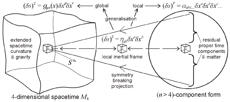
Figure 2: Complementary generalisations of expressions for a proper time interval from the Lorentzian form $(\delta s)^{2}=\eta_{ab}\delta x^{a}\delta x^{b}$: globally to the metric field $g_{\mu\nu}(x)$ underlying a theory gravity and locally to non-quadratic forms with coefficients $\alpha_{abc\ldots}$ providing a basis for matter fields through a local projection over 4-dimensional spacetime $M_{4}$.

Essentially figure 2 describes two complementary generalisations from special relativity: globally for general relativity and locally for the present theory. In general relativity the source of gravitation in the form of spacetime curvature, described by the Einstein tensor $G^{\mu\nu}(x)$ which is a function of the first and second derivatives of the metric $g_{\mu\nu}(x)$, is identified with posited forms of matter, described by the energy-momentum tensor $T^{\mu\nu}(x)$, through Einstein’s field equation:

$$G^{\mu\nu}=-\kappa T^{\mu\nu}$$ (105)

with $\kappa$ a normalisation constant. For the present theory matter itself derives from the complementary local generalisation of a local proper time interval depicted in figure 2. More precisely the properties of the residual components in the projection of the generalised local form of proper time over $M_{4}$ directly shape the spacetime geometry on the extended scale through which the energy-momentum is in turn defined ([54] equation 15.1, [53] equation 85):

$$G^{\mu\nu}\>=\>f(A,\mbox{\boldmath$v$}_{n})\>=:\>-\kappa T^{\mu\nu}$$ (106)

The structure of the spacetime geometry, represented by the function $f(A,\mbox{\boldmath$v$}_{n})$, includes a contribution from gauge fields $A(x)$ via the corresponding field strength tensor $F(x)$, such as the electromagnetic field, in a manner similar to modern Kaluza-Klein theories as reviewed here for equation 32, as well as from subcomponents of $\mbox{\boldmath$v$}_{n}(x)$ of the full form of proper time for equation 15 via the impact of the projected 4-dimensional spacetime component $\mbox{\boldmath$v$}_{4}\in\mbox{\it TM}_{4}$, as described here for equations 29–31 and 40. The quantum properties of matter are proposed to arise as an intrinsic feature through a degeneracy of spacetime solutions for equation 106 ([54] section 10.1, chapter 11 and section 15.2), with quantum particle states exhibiting the properties of equation 66–91 as generalised further for the full form of time proposed for equation 92. In the limit of a flat spacetime approximation, with field dynamics constrained by equation 103, the local interactions of a QFT and quantum particle effects exhibiting the properties of the Standard Model are envisaged to arise from the symmetry breaking projection of the full form for proper time over the local 4-dimensional spacetime. In this manner the properties of ‘corpuscles’ such as electron states, alluding to the second of the above displayed quotes from Einstein, are proposed to be identified from this further generalisation of relativity.

For the Standard Model itself, as usually presented, fields are added to a flat 4-dimensional spacetime background and then quantisation rules applied, completely detached from any consideration of general relativity. This standard theoretical framework reflects the negligible impact of gravity on phenomena recorded in the particle physics laboratory. A more technically challenging approach is needed for any attempt to incorporate gravitation within a theoretical scheme in which quantisation rules are afforded precedence, as for the ambition of string theory – which also aims to accommodate the Standard Model as discussed in subsection 2.1. Here we begin with the very local structure of general relativity and make the generalisation for a proper time interval as depicted in figure 2. Through this unrestricted augmentation, beyond quadratic spacetime forms, matter fields are obtained with features both resembling the Standard Model and also in principle accommodating probabilistic quantum properties through equation 106. Here the nature of gravity is inextricably linked with these properties of matter, without needing to be subsequently appended.

Hence the complete theory is not anticipated to involve classical fields in spacetime which are then ‘quantised’ by applying the postulates of a quantum field theory (such as reviewed in [54] chapter 10), rather the aim is to account for and explain quantum phenomena through this generalisation of the local spacetime structure. Matter, together with its quantum properties, is directly correlated with the spacetime geometry through equation 106, which also describes gravity by incorporating Einstein’s field equation 105 along with an account of the elementary composition of the energy-momentum tensor. The gravitational field $g_{\mu\nu}(x)$ remains an essentially classical field on a smooth spacetime manifold, with no ‘quantisation’ of the spacetime geometry itself. This perspective on quantum theory and particle states is then in a similar spirit to that of the ambition of the early unified field theories as described earlier in this subsection.

As described in subsection 2.2 and earlier in this subsection the present theory can also be motivated in a similar spirit as for the earliest attempts at a unified field theory in that in all cases an assumption concerning the 4-dimensional spacetime metric is dropped, as a possible further progression from the relaxing of the flat spacetime assumption of special relativity that underlies general relativity. For the Weyl, Einstein and Kaluza-Klein theories of equations 3, 4 and 5 for the case of $A_{\mu}(x)=0$ and $F_{\mu\nu}(x)=0$, with vanishing electromagnetic field, the original metric $g_{\mu\nu}(x)$ still describes the curved spacetime of general relativity when related to other matter fields through equation 105. However for the present theory the trivial case of equation 25 corresponds to the matterless vacuum of a flat spacetime, with all matter arising in a manner intrinsically related to the spacetime curvature under augmentations to equation 25 in the form of equation 15 as reviewed above for equation 106.

Although in a similar spirit this approach also differs from the early unified field theories reviewed in subsection 1.2, which were based on a generalisation of the geometry of the global metric $g_{\mu\nu}(x)$ of equation 2 on an extended spacetime, in that here we focus upon the local metric $\eta_{ab}$ of equation 1 of a local inertial reference frame which is generalised to the expression for proper time in equation 13. The embedding of the general metric $g_{\mu\nu}(x)$ in the generalised geometric structures of equations 3, 4 and 5 is analogous to the embedding of the local metric $\eta_{ab}$ within the generalised proper time interval of equation 13 in the manner of equation 14 as described before equation 15. With $\eta_{ab}$ extracted from equation 13 to be locally incorporated into the metric $g_{\mu\nu}(x)$ of general relativity in the extended external 4-dimensional spacetime, matter fields derive from the residual components of the generalised form of time of equation 13 in this projection over the local spacetime geometry as depicted in figure 2.

In a sense the present theory is hence based upon a more elementary generalisation than that of the early unified field theories. Compared with the unified field theories that immediately followed general relativity the shift in focus here towards the local spacetime structure also seems reasonable given the aim of accounting for the microscopic properties of matter. As figure 2 implies we can zoom into an infinitesimal local inertial reference frame anywhere on the spacetime manifold $M_{4}$ and generalise from the form of proper time in equation 1 to explore the microscopic structure of matter that arises. As alluded to in subsection 1.2 the spirit of Einstein’s approach to a unified theory, for example via the generalisation of the global metric components $g_{\mu\nu}\to\tilde{g}_{\mu\nu}$ in equation 4, remains enlightening as can be seen here in the augmentation from the local metric components of equation 1 to the coefficients of equation 13 with $\eta_{ab}\to\alpha_{abc\ldots}$. This approach, which can hence be considered a further generalisation from special and general relativity, has been shown to lead to properties of the Standard Model and beyond as presented in the previous sections. In the following subsection we further emphasise the underlying simplicity of the theory.

5.2 One Simple Equation

As implied in figure 2 the underlying order and structure of matter in spacetime essentially arises from the composition of the continuous flow of time. Through an elementary and direct analysis, from an abstract mathematical perspective, any finite interval of proper time $\Delta s\in{\mathbb{R}}$ can be decomposed down to a limit of infinitesimal intervals:

$$\Delta s = \delta s+\delta s+\delta s+\ldots$$ (107)

$$\quad\mbox{with substructure:}\quad\delta s = {}^{\begin{subarray}{c}p\vspace{1pt}\\ {}\end{subarray}}\!\!\!\!\sqrt{\alpha_{abc\ldots}\delta x^{a}\delta x^{b}\delta x^{c}\ldots}\qquad\qquad\qquad$$ (108)

for $\delta s\to 0$ as the $p^{\mathrm{th}}$-root of a homogeneous polynomial of $p^{\mathrm{th}}$-order in $n$ infinitesimal components $\{\delta x^{a}\}\in{\mathbb{R}}^{n}$ labelled by $a,b,c,\ldots$ with each coefficient $\alpha_{abc\ldots}\in\{-1,0,1\}$, maintaining a consistent order of infinitesimals. Here we are simply exploiting the basic arithmetic properties of the continuum of real numbers, representing the continuum of time with $\delta s\in{\mathbb{R}}$, which together with addition include the operations of multiplication and extracting roots. Equation 108 is equivalent to equation 13, which as a direct generalisation from equation 1 is the starting point for the whole theory.

There is a simplicity in the foundation of this theory in dropping the assumption that a proper time interval should be expressed through a quadratic form, as for equations 1 and 6, and hence generalised to higher-order homogeneous polynomial structures, as described for equation 13. Here we see that this simplification is further emphasised by observing that rather than adding extra spatial dimensions that we do not see, with the components $(\delta x^{4},\ldots,\delta x^{n-1})$ in equation 6, here equation 13 can be interpreted as expressing a basic general arithmetic form inherent in an infinitesimal interval $\delta s$ of the continuum of proper time as described for equations 107 and 108. Hence the theory is essentially grounded conservatively in this ‘one dimension’ of time alone, the passage of which we are intimately familiar with (prompting the title of [54] to emphasise the contrast with theories based on extra spatial dimensions). In equations 13 and 107–108 we are not adding anything to time, nor replacing time with anything, but simply expressing an intrinsic arithmetic substructure that is carried simultaneously with time.

Generally in the equations of physics a lot of attention is naturally paid to the objects on the left-hand side and the right-hand side but the ‘equals sign’ in the middle often carries a significant meaning or interpretation in itself. For example in general relativity the equals sign in Einstein’s field equation 105 is often interpreted to imply that matter (energy-momentum $T^{\mu\nu}$ on the right-hand side) ‘bends’ spacetime (the geometry $G^{\mu\nu}$ on the left-hand side). This description conforms with the historical development since the notion of matter very much preceded the conception of spacetime curvature. However for the present theory the form of the spacetime solution $G^{\mu\nu}\equiv f(A,\mbox{\boldmath$v$}_{n})$ in equation 106 takes priority, with $T^{\mu\nu}$ being defined in terms of this structure in a manner proposed to incorporate the particle and quantum properties of matter consistently with the field equation of general relativity as reviewed in the previous subsection.

Similarly, given the historical background to equation 1 the initial priority might be given to the components of space $(\delta x^{1},\delta x^{2},\delta x^{3})$ and the interval of coordinate time $(\delta x^{0})$ on the right-hand side, since these are effectively assimilated from the earlier Newtonian worldview as alluded to in the previous subsection. In relativity these components are collectively combined in a 4-dimensional spacetime form which can then be identified with the square of the Lorentz invariant proper time interval $\delta s$ on the left-hand side of equation 1. For the present theory, however, we place all the initial emphasis on the left-hand side interval $\delta s$ itself, which can be arithmetically expressed in the quadratic form on the right-hand side of equation 1 and interpreted in geometric terms as a basis for 4-dimensional spacetime.

Consideration of possible arithmetic expressions for the proper time interval $\delta s$ then leads to the general form of equation 13, which is equivalent to the expression for $\delta s$ in equation 108, taken to subsume the 4-dimensional form of equation 1 as described for equation 14. Physical structures arise through the breaking of the symmetry of the full form of time when projected over the 4-dimensional spacetime substructure as depicted in figure 2, leading to properties of matter fields that resemble the Standard Model of particle physics as described in section 3. Hence the pivotal role of the equals sign in equation 1 is central to the interpretation of the theory as deriving entirely from generalising and analysing the single simple entity of proper time.

Attempts to account for all physical phenomena through a single simple entity date back to the pre-Socratic philosopher Thales of Miletus (circa 600 B.C.) on identifying water as the basis for all matter ([93] book 1 chapter 2). As arguably the first ‘unified theory’ this proposal was perhaps motivated on observing that water could be transformed into three known forms, as a solid, liquid or vapour, from which further extrapolation might account for all types of material substances. In light of the apparent empirical implausibility of that theory by the time of Aristotle (circa 350 B.C.) the basic elements had grown to four in number: earth, water, air and fire with a further augmentation by a fifth element, or ‘ether’, originally associated with celestial phenomena. The properties of each element could in turn be ascribed to tiny indestructible atoms of matter, according to the theory of Democritus (circa 400 B.C.), which might be attributed to the unique geometric structures of the five Platonic solids.

In 1808 John Dalton proposed the modern atomic theory of matter with chemical combinations of originally around twenty elements, including hydrogen, carbon and oxygen, in simple numerical ratios accounting for the wide variety of compound substances. By 1869 the list had grown to over sixty basic elements which when ordered according to their atomic weights were seen to exhibit recurring physical properties at a regular pattern of intervals in Mendeleev’s Periodic Table of chemical elements. By that time the ‘ether’ had been reinvented as the ‘luminiferous ether’ proposed to permeate all space, with elastic mechanical properties permitting the transmission of light similarly as vibrations in the air allow the propagation of sound. However such a hypothetical ethereal medium substratum for the electromagnetic field in Maxwell’s theory [20], discussed here in subsection 1.2, or an ‘ether drift’, was never detected and that concept along with the notion of a Newtonian absolute space with which to associate such an ether was ultimately discarded as superfluous with the advent special relativity in 1905 ([23] introduction).

The regular pattern of Mendeleev’s Periodic Table of chemical elements hinted at an inner structure for atoms that foreshadowed the discovery of their composition and quantum properties, as alluded to in the opening of section 1. The 1911 Rutherford model of subatomic structure with a central massive nucleus surrounded by a spherical cloud of electrons was followed by the 1913 Bohr atom with the electrons confined to circular orbits in discrete steps of angular momentum in multiples of Planck’s constant as an application of the ‘old quantum theory’ ([24] chapters 9 and 10), subsequently supplanted by the atomic picture of the ‘new quantum theory’ in the mid-1920s ([24] chapter 12). By 1925 in addition to the two established fundamental forces of electromagnetism and gravitation only the electron, proton (identified with the hydrogen nucleus) and photon were believed to be needed to account for elementary material phenomena, albeit with a third force seemingly required to hold the atomic nucleus together ([24] section 12(a)). The empirical study of the properties of those and further components discovered over the following half a century led to the Standard Model of particle physics as established by 1975. With the Standard Model incorporating a collection of regular symmetry patterns associated with multiplets of elementary particles the focus then turned to the empirical and theoretical investigation into the underlying source of these structures.

In the late 19^th and early 20^th century gaps were filled in and the Periodic Table grew in size with the discovery of further chemical elements, before an underlying explanation in terms of atomic structure was uncovered. Similarly since 1975 the Standard Model has been both confirmed with new empirical discoveries and augmented with an extended neutrino sector and other models of physics beyond, while the search continues for an explanation of the origin of these properties.

Rather than conceiving of the composition of the world as an indefinite sequence of ‘onion layers’ of comparable complexity the intuitive idea is often expressed that the underlying structure of matter is expected to become simpler as deeper layers are explored. On the macroscopic scale a huge variety of elaborate material structures can be observed. While a great deal of complexity remains for structures that can be observed with the most powerful optical microscopes all such matter is composed from a wide range of molecules and compounds in turn constructed from combinations of less than a hundred chemical elements. As arranged in the Periodic Table these elements are associated with a series of basic atomic structures built from a common set of a small number of component types. Analysis of these components led to the discovery of a range of elementary particles, somewhat smaller in number than the variety of atoms, as arranged in the Standard Model. The thread of ever greater simplicity is proposed here to culminate in equations 107 and 108, with the basic arithmetic decomposition of time itself providing the template for the elementary particle multiplet structures. The distinctive patterns of the Standard Model arise from the symmetry of the generalised multicomponent form of time as this symmetry is broken in the projection over the local geometric form of 4-dimensional spacetime as described for figure 2.

Atoms listed in the Periodic Table can be broken down into constituent pieces while in other experiments the particle states of the Standard Model can mutate into each other through interactions. Seemingly no such experiment can be performed for ‘time’ as the basic element of the present theory. However time can be ‘broken down’ and ‘mutated’ through the simple mathematical analysis and identities of equations 107 and 108. Indeed it is precisely through this analysis that substructures of time can be identified as a basis for both the geometry of 4-dimensional spacetime and the matter content within this arena as studied in the laboratory as described explicitly in subsection 3.1. In this sense particle physics experiments could be considered as an investigation into the elementary substructure of time itself. Since it is difficult to conceive of a simpler basis for a theory than time alone, and since the ‘fragmentation’ of this entity in equations 107 and 108 is already employed at the heart of this theory, there is a sense of reaching the ultimate ‘bedrock’ in accounting for the properties of matter, with no further ‘onion layers’ to be sought at a yet deeper level.

On the other hand given equation 108, which is equivalent to equation 13 and can be conveniently written in the form of equation 15, specific mathematical possibilities for this generalisation of proper time and their empirical consequences are very much open to further exploration. This has been described through to the proposed level of an $\mbox{E}_{8}$ symmetry in subsection 3.2 with tentative consequences for physics beyond the Standard Model considered in section 4, demonstrating the potential of this theory for making testable predictions. The possibility of a yet higher-order fragmentation for equation 108, with potentially fractal-like properties, or a role for alternative multicomponent forms for proper time as suggested for equation 104 as a candidate source of a dark sector in subsection 4.2, can also be considered.

The flow of time pervades the entire spacetime manifold in figure 2, sharing this property with the hypothetical ether. However, while the ether was abandoned with relativity theory the notion of proper time, and its local invariance, is central to the progression through special and general relativity to the theory presented here, as described in the previous subsection. For Maxwell the luminiferous ether, while never detected, was a postulated material substratum underlying the observed phenomena of the electromagnetic field. Here on the other hand there is no question of performing an experiment to search for ‘time’, rather we are directly and intimately familiar with the flow of time as an irreducible element infusing all experiments and observations, including in the high energy physics laboratory, with all particle and material phenomena proposed to arise through the substructure of time.

Indeed the usual basis for most physical models and theories is to begin by positing a basic entity or entities in space and time, whether for example water, an ether, atoms, particles or fields. Here the left-hand sketch in figure 2 is not ultimately to be similarly interpreted with the basic entity time $s$ flowing through a pre-existing space and time. Rather the geometric spacetime structure itself, as well as the matter within it, is extracted through the composition of the continuum of time as the sole basic entity. While conceptually very different to earlier unification schemes, the simplicity of this perspective then provides a further motivation for the theory. The historical and philosophical aspects associated with this simple interpretation of the theory as deriving from the intrinsic arithmetic substructure of proper time alone are elaborated in [94]. In particular this change in perspective with time promoted to the prior role, via the substructure of equations 107 and 108, as the progenitor for both spacetime structure and matter in spacetime, subject to laws of physics determined by the constraints implied by this underlying simplicity, is further described for ([94] figure 1).

The properties of elementary particles are uncovered at the most elementary level of the theory through a simple symmetry breaking analysis for equation 108, written as equation 15, deriving directly from the extraction of an external $\mbox{Lorentz}\subset\hat{G}$ symmetry acting on the projected $\mbox{\boldmath$v$}_{4}\in\mbox{\it TM}_{4}$ subcomponents of $\mbox{\boldmath$v$}_{n}\in{\mathbb{R}}^{n}$ that underlie the basis of the local external 4-dimensional spacetime itself, without adding anything else to the theory. This symmetry breaking is implied through the necessity of perceiving a physical world in space as well as through time, as also discussed in ([94] section 4), with the properties of matter entirely determined by the residual components in the form for proper time of equation 15 over the 4-dimensional spacetime manifold $M_{4}$.

As noted above this contrasts with the usual approach of formulating a theory through the introduction of entities with particular properties into a pre-existing space and time. Such is the case for example in Maxwell’s theory with the introduction of electric and magnetic fields, whether or not supported by an ethereal substratum, together with a set of equations to describe empirical observations. In many modern-day theoretical frameworks particle properties are typically built in by hand in a similar spirit as for Maxwell’s theory by introducing the corresponding fields and interactions into the proposed Lagrangian for the theory, as is the case for the ‘Standard Model’ itself as well as typically for many models beyond. While masses and charges are assigned to physical bodies in the equations of gravitation and electromagnetism of Newton and Maxwell, similarly in the Lagrangian of the Standard Model masses, charges and couplings generally for elementary particles are typically assigned according to empirical observations.

There are a number of constraints on the type of fields and terms that can be included in a Lagrangian. This is particularly the case in the context of a quantum field theory (the postulates of which are also generally imposed pragmatically) for consistency with unitarity and causality. Typically the Lagrangian will be a real function consisting of a series of terms in the fields and their first or second order derivatives in a Lorentz and gauge invariant form, with the renormalisability of the QFT placing further restrictions such as avoiding coupling constants with negative mass dimension. Nevertheless considerable arbitrariness is still permitted, particularly for the construction of models beyond the Standard Model. Indeed on occasions when a provisional hint of new physics is seen in the high energy physics laboratory, in data otherwise implying a significant statistical fluctuation above the expected background, a large number of new models may be prompted as there will generally be many ways to accommodate the apparent observations through augmenting the Standard Model Lagrangian. Even for the Standard Model, with a minimal extension to incorporate the current phenomenology of left-handed neutrinos, at least 25 free parameters also need to be introduced and determined or constrained from the data (eighteen for the Standard Model together with seven neutrino mass and mixing parameters).

In the light of these observations the sentiment is sometimes expressed that a key ambition for a unification scheme would be to replace the lengthy and complicated Lagrangian of the Standard Model by ‘one simple equation’ from which all of the properties of particle physics might be derived. A number of questions could be raised about any candidate for such a primordial equation, with key issues regarding the nature of the basic entity described, whether for example a particle, field, string etc., concerning why it should exist itself at all, why it should be the basic entity and why it should be subject to the ‘one simple equation’.

For the present theory ‘time’ is the basic entity. As well as being fundamental to empirical and theoretical physics, as discussed in this section, time is also a necessary, intrinsic and inherent element of any subjective experience we can have, unlike the case for water, an ether, atoms, particles, fields or other proposed basic physical entities. These fundamental objective and subjective features of time make it an appropriate basic element for any theory. For the present theory time is the sole basic entity. Further, here we are not proposing or positing an equation to be imposed on time, rather we are simply utilising a direct arithmetic property innate in the concept of the continuum of time as expressed for equations 107 and 108.

The continuum properties of time have been recognised as central to the development of the equations of physics in describing the behaviour of matter since the days of Newton, as noted in leading up to figure 2 in the previous subsection. Here however we do not introduce any material or other entity with a particular ‘time dependence’, rather material phenomena derive from the ‘subcomponents of time’ itself through equation 108, which also accommodates the basis for the local Lorentz metric structure of the background spacetime arena via the substructure of equation 14. In this manner all of physics is proposed to follow from the ‘one simple equation’ for the invariant proper time interval $\delta s$ in equation 108, which is equivalent to equation 13 and can be written as equation 15 as described in subsection 2.2, as the basis of the theory. As labelled in equation 15 the symmetry transformations applied to the subcomponents of time belong to a group $\hat{G}$ that generalises the Lorentz group of relativity theory.

A connection with the Lagrangian approach is anticipated to arise through terms in the breaking of the full symmetry $\hat{G}$ of equation 15 in the projection over the local substructure of 4-dimensional spacetime $M_{4}$. Matter fields deriving from the broken fragments of $\mbox{\boldmath$v$}_{n}\in{\mathbb{R}}^{n}$ will feature in ‘mass terms’ in the resulting expression of equation 40 if composed with a factor derived from the projected subcomponent $\mbox{\boldmath$h$}\equiv\mbox{\boldmath$v$}_{4}\in\mbox{\it TM}_{4}$, which is here central to the ‘origin of mass’ itself and associated with the Higgs as described for equations 29–31, with Yukawa coupling factors to be identified as proposed in subsection 4.2. The broken symmetry expression in equation 40 also places constraints on the dynamics of the matter fields, coupling them with gauge fields, as discussed in subsection 2.3. The role of Lagrangian kinetic terms for each gauge field $A(x)$ associated with the internal symmetry is proposed to be appropriated by the quadratic terms in the internal gauge curvature $F(x)$ in the relation with the external spacetime geometry of equation 32, which is similar to that in many Kaluza-Klein theories, with the dynamics of the gauge fields constrained by geometric identities as also reviewed in subsection 2.3. Further, rather than applying the postulates of a quantum theory, a local degeneracy of field solutions for describing the external spacetime geometry is proposed to underlie the ‘quantisation’ of the matter and gauge fields and the corresponding particle phenomena as reviewed for equation 106.

That these particle phenomena will exhibit properties closely resembling the Standard Model has been demonstrated for the analysis through to the $\hat{G}=\mbox{E}_{7}$ level of equation 66–91 in subsection 3.1. The full picture is predicted to emerge for the proposed $\hat{G}=\mbox{E}_{8}$ level of equation 92 as discussed in subsection 3.2, for which physics beyond the Standard Model in the neutrino, Higgs and dark sectors can be anticipated as described in section 4. It is striking to observe how properties of the Standard Model, and contemporary physics beyond, can be uncovered in this manner from such a simple underlying basis. In particular the above analysis illustrates how a range of relatively complex phenomena, matching empirical observations, can be obtained through the ‘one simple equation’ for an infinitesimal interval of time in equation 108, or the equivalent expressions of equations 13 and 15. The ultimate ambition would be to determine not only the elementary particle multiplet structure but also the masses, charges and couplings of elementary particle states as far as possible from the intrinsic constraints of the theory. In deriving from the natural generalisation for a proper time interval in equation 108 as a simple elementary basis for the theory, there is then the potential for a genuine understanding of the underlying origin of the Standard Model and physics beyond, all accounted for by a fundamental unified theory.

6 Discussion and Conclusions

One of the main aims of experiments in particle physics, observations in cosmology and the construction of phenomenological models, typically via a proposed Lagrangian function, is to point the way to a unified theory incorporating a more elementary understanding of the workings of the universe. Given a set of empirical data and an array of associated models an intuitive leap, rather than a series of small iterative steps, is likely to be needed to uncover the fundamental theory. Having posited such a theory, based largely on an internal motivation relating to its conception, the aim would then be to work forwards developing the theory and seeking correspondence with models that have been devised on the basis of empirical observations. In this paper we are not building a model pragmatically, for example by adding terms to a Lagrangian by hand, but rather we have posited such a fundamental theory and developed the consequences from underlying elementary first principles.

In place of directly adding matter fields independently on top of 4-dimensional spacetime to match empirical observations, as for the models alluded to above, the early approaches to a unified field theory reviewed in subsection 1.2 aimed to account for the empirical properties of matter in spacetime within a single unified framework by further generalising the structure of spacetime itself. This principal goal was present from the beginning, as alluded to in the title of Kaluza’s paper [35], and continues to motivate modern-day unification schemes with extra spatial dimensions aiming to account for the Standard Model through an augmented spacetime structure. Via such a conception the aim has been to achieve a unification in which the field and particle states we observe in experiments reside within the internal ‘mathematical space’ of extra spatial dimensions, which is more akin to the external ‘geometrical space’ within which macroscopic structures such as ourselves reside and through which we perceive the physical world.

Extra spatial dimensions have then provided the potential to connect the physics of the external world of 4-dimensional spacetime and the internal world of material phenomena within a more unified structure (see for example [37] section 9 first two of final three paragraphs). However even the most sophisticated attempts to account for the Standard Model via the structures of extra spatial dimensions, as discussed in subsection 2.1, have if anything been less successful than the original 5-dimensional spacetime theory of Kaluza and Klein in accommodating electromagnetism, as reviewed for equation 5.

From a local perspective the addition of extra spatial dimensions augments a proper time interval $\delta s$ from the form of equation 1 to that of equations 6 and 7, as depicted by the generalisation from figure 1(a) to 1(b). An elementary analysis for the implied matter content in 4-dimensional spacetime is described for equation 8–11. The present theory is based on a direct further generalisation of a proper time interval over and above the 4-dimensional form of equation 1 for the local external spacetime to the form of equation 13. Compared with augmentations restricted to extra spatial dimensions with the quadratic form of equation 6 the more general homogeneous polynomial form of equation 13 demands fewer assumptions, as explained in subsection 2.2. As described explicitly for equation 14 this more generalised form for proper time can still readily accommodate a substructure matching the local external spacetime metric geometry.

Adopting the generalisation of equation 13, which can be expressed as equation 15, matter fields are then associated with the properties of the residual components resulting from the symmetry breaking of the generalised form of proper time when projected over the local 4-dimensional geometric spacetime substructure, as depicted in figure 2. The elementary physical structures identified in spacetime for a minimal case are described in subsection 2.3. Leading to the structure of equation 66–91 the residual components are found to exhibit a significant correlation with the Standard Model of particle physics as reviewed in section 3. This direct analysis for the general form of proper time then provides a far better template for connecting with the Standard Model, and with features beyond as described in section 4, than the equivalent analysis applied for the restricted case of extra quadratic spatial components as described for equation 8–11, and in this respect also compares favourably with the more sophisticated approaches to extra spatial dimensions discussed in subsection 2.1.

Similarly as for extra spatial dimensions this theory based on generalised proper time can be seen as a natural further development from special and general relativity as described in subsection 5.1. Compared with the employment of extra spatial dimensions the present theory is however more unifying in reducing the fundamental entity of theory to the more elementary starting point of the single parameter of proper time alone. The greater simplicity of the theory is manifested in its expression through ‘one simple equation’ for infinitesimal intervals of time as discussed in subsection 5.2 for equation 108, which is equivalent to equations 13 and 15. The theory is also more conservative in that the flow of time is something that we are intimately familiar with while, essentially by definition, we do not perceive any ‘extra’ spatial dimensions. Further the theory is more unique in terms of having an unambiguous starting point in proper time as parametrised by $s\in{\mathbb{R}}$ with a trivial topology, rather than having a potentially arbitrary number of extra spatial dimensions with a large range of possible topological properties. This uniqueness is further seen in the mathematical development of the theory in leading to equations 65–91, as summarised in the opening of subsection 3.2. Each of the above points applies for the present theory both in comparison with the direct approach to extra spatial dimensions of equations 6–11 and figure 1 as well as in comparison with the most technically sophisticated approach via string and M-theory which, for example with regards to uniqueness, is faced with the landscape problem as also discussed in subsection 2.1.

The internal simplicity and uniqueness of the present theory, which nevertheless yields a far more direct and efficient connection with empirical structures of the Standard Model at the most elementary level of matter compared with the models based on extra spatial dimensions, strongly suggests that equation 15 rather than equation 7 provides a more appropriate core basis for a unified theory. The extraction of a necessarily quadratic substructure to represent the local external spacetime also underlies a mechanism for the symmetry breaking itself for equation 15 but not for equation 7, as described after equation 16. While models with extra spatial dimensions essentially propose a ‘materialisation of space’ the present theory goes further by describing a ‘materialisation and spatialisation of time’. The nature of our necessary perception of the world in space as well as through time is central to the symmetry breaking as also alluded to in subsection 5.2 with reference to [94] where further historical background to this conceptual picture is also discussed. Here we briefly summarise the historical developments in mathematics and physics underlying this theory.

The first particle of the Standard Model to be discovered was the electron at the end of the $19^{\mathrm{th}}$ century, around the same time that the exceptional Lie algebras were first classified as noted in the opening of subsection 3.1. The Standard Model itself was fully established in the 1970s, representing an amalgamation of the inferences drawn from many experiments over a number of decades, and has been tested subsequently and largely confirmed by further decades of empirical data through to the discovery and analysis of the Higgs in recent years. Mathematical developments from the mid-$20^{\mathrm{th}}$ to early $21^{\mathrm{st}}$ century, including [57, 58, 59, 60] as cited in subsection 3.1, have enabled the development of the present theory, as expressed for equation 15, through the 9, 27 and 56-dimensional forms of equations 26, 48 and 65. These have led respectively to the identification of the symmetry breaking structures of equations 33–38, 50–64 and 66–91, closely resembling the features of a generation of Standard Model leptons and quarks – including a set of spinor states, colour $\mbox{SU}(3)_{c}$ singlets and triplets with the appropriate electromagnetic $\mbox{U}(1)_{Q}$ fractional charges and an intrinsic left-right asymmetry.

This progression then represents an intimate coming together of mathematical and physical structures which, while contemporary with each other and studied in parallel, developed largely independently over the past hundred or more years, and with very little redundancy as seen for equation 66–91, drawn together through natural mathematical expressions for equation 15 as the central equation of this unified theory. While the theory is rooted in the firm conceptual basis of generalised proper time the subsequent employment of mathematical structures relating to the exceptional Lie groups has advanced the theory to the point of making connections with empirical phenomena. Mutually, the application of these mathematical structures, which have been developed in a largely abstract manner, within the context of the present theory, presents an explicit means of relating the exceptional Lie groups to the physical world. That is, the expressions in equations 48 and 65 provide their respective symmetry groups $\mbox{E}_{6}$ and $\mbox{E}_{7}$ with a clear and simple conceptual basis within this theory, as symmetries of generalised proper time, without needing to introduce them in an ad hoc fashion as might be the case for model building (dating back to [32, 33] as alluded to in subsection 1.2), here making their relevance for the Standard Model explicit through equations 50–64 and 66–91. Such an interplay of mathematical development and physical application is analogous to the incorporation of fibre bundle structures in the framework of gauge theories and non-Abelian Kaluza-Klein theories as discussed in subsection 1.2 with reference to [37, 38].

While properties associated with the Standard Model emerge much more readily for the present theory, compared to models with extra spatial dimensions, a complete correspondence is not to be expected until a mathematically complete understanding of the full form of proper time, and its corresponding symmetry breaking pattern, has been established. The unique development of the theory through to the $\mbox{E}_{7}$ quartic form of equation 65 with the implications of equation 66–91 together with properties of the exceptional Lie groups naturally lead to the prediction of a further unique progression to an $\mbox{E}_{8}$ symmetry of a full form $L_{8}(\mbox{\boldmath$v$}_{248})_{\mathrm{E}_{8}}=1$, as described for equation 92 in subsection 3.2, proposed to result in the uncovering of the full particle multiplet structure of the Standard Model and beyond. While elements of the Standard Model have been accounted for through a rigorous analysis of the $\mbox{E}_{6}$ and $\mbox{E}_{7}$ levels underlying equations 50–64 and 66–91, the investigation at the $\mbox{E}_{8}$ level, including that for equation 102, has to date been of a more provisional nature. An explicit description of a real $\mbox{E}_{8}$ action constructed on the, currently hypothetical, homogeneous form of equation 92 with a symmetry breaking pattern of equation 93 applied to the subcomponents of $\mbox{\boldmath$v$}_{248}\in{\mathbb{R}}^{248}$, subsuming equation 66–91, will be needed to attempt a full reconstruction of the Standard Model structure and to make firm predictions beyond.

The need to unfold the full Standard Model structure, including three generations of leptons and quarks with a complete set of spinor states also for the $\nu$-leptons and $u$-quarks and with a full electroweak symmetry, implies that there are significant requirements on the desired structure of the homogeneous polynomial form $L_{8}(\mbox{\boldmath$v$}_{248})_{\mathrm{E}_{8}}=1$ which may also be utilised as a guide in identifying the $\mbox{E}_{8}$ symmetry structure and breaking pattern itself. However the main goal for the predicted $\mbox{E}_{8}$ structure, as achieved for the intermediate $\mbox{E}_{6}$ and $\mbox{E}_{7}$ levels, is principally to deduce the properties of the Standard Model, and beyond, as constrained by the natural mathematical expressions for equation 15. That it is not obvious that this can be achieved for $\mbox{E}_{8}$, or a closely related symmetry structure consistent with equation 15, provides a non-trivial test for the theory. The technical mathematical details of the connections with the Standard Model made through to the $\mbox{E}_{7}$ level and support for the predicted role for $\mbox{E}_{8}$ are described extensively in [53] and the references therein. Here a significant direction for further progress on the mathematical side, through investigating a possible role for octonion triality in the construction of an octic $\mbox{E}_{8}$ invariant in 248 components, has been described in subsection 3.2 – in particular with the guide of the references cited in the last three paragraphs of that subsection.

The attempt to advance the status of the theory beyond the conceptual basis and corresponding mathematical formalism by making connections with empirical phenomenology has also been extended beyond the Standard Model. In this paper we have focussed upon the opportunity for a mutual development of this theory along with an understanding of new physics, in particular in the neutrino sector. Building upon the progression through the $\mbox{E}_{6}$ and $\mbox{E}_{7}$ levels general consideration of the possibility of a significant role for $\mbox{E}_{8}$ leads, via the schematic extrapolation from the relevant parts of equations 50–64 and 66–91 to equation 102, to the preliminary prediction for only two right-handed neutrino states to be accommodated in a manner compatible with a structure of three generations for the other lepton and quark states. As also noted in subsection 4.1 this suggests that one of the active left-handed neutrino states will be correspondingly massless, with forthcoming improving limits in the laboratory and from cosmology able to test this tentative but specific empirical feature of the theory. By making a connection with models featuring two right-handed neutrinos (for example [13, 14, 15, 16]) in this paper the focus has been to demonstrate a specific bridge from the forefront in developing this theory, based on a very simple underlying origin, to a key area in recent developments in particle physics.

If this theory had reached the present stage of development in the 1980s, with the Standard Model established but still with relatively limited empirical input in neutrino physics, then the argument for two right-handed neutrinos would not have been a compelling prediction of the theory at this point. Rather we have aimed to demonstrate how the theory might in principle accommodate two right-handed neutrinos naturally within a structure of three generations of Standard Model fermions, consistent with a series of recent neutrino models that have been motivated by contemporary neutrino phenomenology. While at this stage lacking in more explicit detail for the neutrinos, since the present theory is based on elementary first principles rather than being explicitly tailored to fit the data as a pragmatic model, through further development there is here an opportunity for a deeper understanding of the nature of neutrino physics generally, as discussed in subsection 4.1.

While the mathematical pursuit of the full symmetry action of $\mbox{E}_{8}$ for the form $L_{8}(\mbox{\boldmath$v$}_{248})_{\mathrm{E}_{8}}=1$ and the resulting breaking pattern may elucidate the origin of the esoteric properties of the neutrino sector, building upon the basic generation structure of equation 102, existing empirical knowledge of neutrino phenomenology as established in recent decades, as expressed by models with two right-handed neutrinos (or even other models such as for example the $\nu$MSM in which two right-handed neutrinos have distinct properties and a distinct role from a third $\nu_{R}$ state [7, 8] as also reviewed in subsection 1.1), might itself provide a pertinent clue, on top of the Standard Model itself, towards deciphering the detailed structure of the specific mathematical application for $\mbox{E}_{8}$ that is predicted. In particular the packing of the neutrino spinor structure, under an $\mbox{SL}(2,{\mathbb{C}})\subset\mbox{E}_{8}$ action of equation 93 on the subcomponents of $\mbox{\boldmath$v$}_{248}$ in equation 92 utilising octonion triality as alluded to above, and their Dirac or Majorana nature in mass terms identified in the expansion of equation 103, will be central to this ambition. A connection might then be made between Lorentz and gauge invariant terms in the expansion of equation 103 and Lagrangian mass terms in models with two $\nu_{R}$ states. More generally there is an open opportunity to explore the mutual development and close interplay of the underlying mathematical structure of the theory together with an understanding of Standard Model physics and empirical consequences beyond.

The main approach of this theory is ‘deductive’ in starting with the hypothesis of the central role for proper time in equations 13 and 15 and then developing the mathematics, for example through to equations 66–91 and 102, to then examine the empirical consequences in a manner ideally leading to testable predictions. As alluded to in the opening of this section this contracts with the ‘inductive’ approach employed in the construction of a model, as inferred from patterns in the data, for example by adding fields and terms to a Lagrangian. While that data hence provides evidence for such a model the inductive argument is not in general unique and typically leads to a range of plausible models, as is generally the case for neutrino phenomenology. Here, while an interplay with inductive elements might be utilised to aid in the mathematical construction of the $\mbox{E}_{8}$ action and the explicit form of equation 92 sought, the ultimate aim is for a clear, unique and deductive argument unambiguously covering a wide range of physical phenomena, and for example homing in on the features of a particular model in the neutrino sector.

A degree of confidence in any predictions of the theory can be gained through the intrinsic simplicity of the underlying basis of the theory, as described in the previous section, and the significant foothold in features of the Standard Model that has already been efficiently attained as summarised here for equations 33–38, 50–64 and 66–91. Indeed most of the subcomponents of $\mbox{\boldmath$v$}_{56}$ in equation 66–91 are associated with elements of the Standard Model with the only apparent redundancy being the set of four scalar invariants $\{n,N,\alpha,\beta\}$, which provisionally form candidates for dark matter as described in the opening of subsection 4.2. The prospects for insights into new physics include the nature of the Higgs and electroweak symmetry breaking, for which empirical predictions might be sought for the laboratory. The close connection here between the Higgs sector, associated with the $\mbox{\boldmath$h$}\equiv\mbox{\boldmath$v$}_{4}\in\mbox{\it TM}_{4}$ projection of equations 29 and 30, and neutrino physics, as implied by equation 102, suggests the Higgs may have a composite structure as described in subsection 4.1. This feature, together with the possible connections between this Higgs and a dark sector as explained in subsection 4.2, may impact precision electroweak measurements in a manner accessible at the LHC or at a future $e^{+}e^{-}$ linear collider as also discussed in section 4.

In subsection 4.2 we described for equation 104 how the impact of possible alternative forms for proper time on the 4-dimensional spacetime geometry might itself provide a quintessential source for the dark sector, in only being linked with the visible sector deriving from the $\mbox{E}_{8}$ form of equation 92 through purely gravitational means. Correspondingly the generalisation from $\{n,N,\alpha,\beta\}$ at the $\mbox{E}_{7}$ level of equation 66–91 could yield a broader set of scalar invariants under the full $\mbox{E}_{8}$ broken symmetry which, on taking vacuum values and being composed in terms of the expansion of equation 103, may form a range of Yukawa couplings and hence in principle augment the predictive power of the theory, as also noted in subsection 4.2. More generally analysis of the properties of the full set of subcomponents of $\mbox{\boldmath$v$}_{248}\in{\mathbb{R}}^{248}$ from the breakdown of equation 92 offers the opportunity to explore further new physics, as does the possibility to fit a further gauge group alongside that of the Standard Model in the $\mbox{E}_{8}$ symmetry breaking pattern of equation 93.

While previous papers (including [39, 53]) have described in detail the connections made with the Standard Model (summarised here in section 3), in this paper we have emphasised the potential connections with new physics (as assessed in section 4), while always keeping in sight the simple origins of the theory based on an elementary generalisation of a proper time interval as described for equations 13 and 15. With reference to subsection 1.2, in section 2 and subsection 5.1 we have described how the basis for this theory connects with the early unification schemes from the immediate post-general relativity era based on generalisations of the 4-dimensional spacetime geometry. Hence in developing the present theory we connect the original conception of a unified field theory dating from a hundred years ago with the current quest to understand the empirical data from recent and ongoing laboratory experiments and cosmological observations. In particular the modern-day empirical status of neutrino physics, as reviewed in subsection 1.1, is hence connected with the historical proposals of subsection 1.2 through this theory, ultimately making contact with models featuring two right-handed neutrinos as explained in subsection 4.1 (with the central argument summarised in [1]).

As described for equations 107 and 108 it is difficult to conceive of a more elementary basis for a unified theory than this simple direct generalisation of proper time. On the other hand the natural mathematical possibilities for the invariant infinitesimal proper time interval in equation 108, which is equivalent to the ‘one simple equation’ of equation 13 and also equation 15, are open to further exploration. Also open to investigation are the wider implications of the theory in relation to the geometric structures of Kaluza-Klein models [40], quantisation and the nature of physical particle states as studied in laboratory experiments ([54] chapters 10, 11 and section 15.2, as also discussed for [94] equations 9 and 10) and the cosmological questions regarding the dark sector and early universe ([54] chapters 12 and 13) as well as the connections with the Standard Model itself ([54] chapters 6–9, [39, 53]). With the aim of making a range of testable predictions there is an opportunity for mutual advances in these theoretical and related experimental investigations. The manner in which this theory has been able to reproduce a series of key features of the Standard Model, and has already yielded provisional connections with neutrino and other new physics beyond, demonstrates this open opportunity to further explore this theoretical structure with the ambition of advancing our understanding of the elementary constitution of the physical world.

References

- [1] D. J. Jackson, ‘From Unified Field Theory to the Standard Model and Beyond’, arXiv:1809.05403 [physics.gen-ph] (2018).
- [2] M. Tanabashi et al. [Particle Data Group], ‘Review of Particle Physics’, Phys. Rev. D 98 (3), 030001 (2018), [available at http://pdg.lbl.gov].
- [3] M. Drewes, ‘The Phenomenology of Right Handed Neutrinos’, Int. J. Mod. Phys. E 22, 1330019 (2013) [arXiv:1303.6912 [hep-ph]].
- [4] J. Wolf [KATRIN Collaboration], ‘The KATRIN Neutrino Mass Experiment’, Nucl. Instrum. Meth. A 623, 442–444 (2010) [arXiv:0810.3281 [physics.ins-det]].
- [5] N. Aghanim et al. [Planck Collaboration], ‘Planck 2018 Results. VI. Cosmological Parameters’, arXiv:1807.06209 [astro-ph.CO] (2018).
- [6] M. Agostini, G. Benato and J. Detwiler, ‘Discovery Probability of Next-Generation Neutrinoless Double- Decay Experiments’, Phys. Rev. D 96 (5), 053001 (2017) [arXiv:1705.02996 [hep-ex]].
- [7] T. Asaka, S. Blanchet and M. Shaposhnikov, ‘The MSM, Dark Matter and Neutrino Masses’, Phys. Lett. B 631, 151 (2005) [arXiv:hep-ph/0503065].
- [8] T. Asaka and M. Shaposhnikov, ‘The MSM, Dark Matter and Baryon Asymmetry of the Universe’, Phys. Lett. B 620, 17 (2005) [arXiv:hep-ph/0505013].
- [9] P. Mermod [SHiP Collaboration], ‘Right-Handed Neutrinos: the Hunt is on!’, Proc. of NuPhys2016, London (12–14 Dec. 2016), arXiv:1704.08635 [hep-ex].
- [10] P. Di Bari, ‘Right-Handed Neutrinos in Cosmology: Light Versus Heavy’, Nucl. Phys. B (Proc. Suppl.) 168, 41–43 (2007).
- [11] A. Boyarsky, M. Drewes, T. Lasserre, S. Mertens and O. Ruchayskiy, ‘Sterile Neutrino Dark Matter’, Prog. Part. Nucl. Phys. 104, 1 (2019) [arXiv:1807.07938 [hep-ph]].
- [12] D. Döring, H. Päs, P. Sicking and T. J. Weiler, ‘Sterile Neutrinos with Altered Dispersion Relations as an Explanation for the MiniBooNE, LSND, Gallium and Reactor Anomalies’, arXiv:1808.07460 [hep-ph] (2018).
- [13] P. H. Frampton, S. L. Glashow and T. Yanagida, ‘Cosmological Sign of Neutrino Violation’, Phys. Lett. B 548, 119 (2002) [arXiv:hep-ph/0208157].
- [14] A. Ibarra and G. G. Ross, ‘Neutrino Phenomenology – The Case of Two Right-Handed Neutrinos’, Phys. Lett. B 591, 285–296 (2004) [arXiv:hep-ph/0312138].
- [15] S. Antusch, P. Di Bari, D. A. Jones and S. F. King, ‘Leptogenesis in the Two Right-Handed Neutrino Model Revisited’, Phys. Rev. D 86, 023516 (2012) [arXiv:1107.6002 [hep-ph]].
- [16] C. C. Li and G. J. Ding, ‘Implications of Residual Symmetry for Leptogenesis in a Model with Two Right-Handed Neutrinos’, Phys. Rev. D 96 (7), 075005 (2017) [arXiv:1701.08508 [hep-ph]].
- [17] M. Fukugita and T. Yanagida, ‘Baryogenesis without Grand Unification’, Phys. Lett. B 174, 45 (1986).
- [18] P. Di Bari, ‘An Introduction to Leptogenesis and Neutrino Properties’, Contemp. Phys. 53 (4), 315 (2012) [arXiv:1206.3168 [hep-ph]].
- [19] Y. Shimizu, K. Takagi and M. Tanimoto, ‘Neutrino Violation and Sign of Baryon Asymmetry in the Minimal Seesaw Model’, Phys. Lett. B 778, 6 (2018) [arXiv:1711.03863 [hep-ph]].
- [20] James Clerk Maxwell, ‘A Dynamical Theory of the Electromagnetic Field’, Phil. Trans. Roy. Soc. Lond. 155, 459–512 (1865).
- [21] Albert Einstein, ‘The Foundation of the General Theory of Relativity’, Annalen Phys. 49 (7), 769–822 (1916) [Annalen Phys. 14 (Supplement), 517–571 (2005)], translated by Alfred Engel in ‘The Collected Papers of Albert Einstein’ 6, 146–200, Princeton University Press (1997).
- [22] Abraham Pais, ‘ “Subtle is the Lord…”: The Science and the Life of Albert Einstein’, Oxford University Press (1982, 2005).
- [23] Albert Einstein, ‘On the Electrodynamics of Moving Bodies’, Annalen Phys. 17, 891 (1905) [Annalen Phys. 14, 194 (2005)], translated by Anna Beck in ‘The Collected Papers of Albert Einstein’ 2, 140–171, Princeton University Press (1989).
- [24] Abraham Pais, ‘Inward Bound: Of Matter and Forces in the Physical World’, Oxford University Press (1986, 1988, 1994).
- [25] Hermann Weyl, ‘Gravitation and Electricity’, Sitzungsber. Preuss. Akad. Wiss. Berlin (Math. Phys.) 1918, 465 (1918).
- [26] Hermann Weyl, ‘Space Time Matter’, translated by Henry L. Brose, Dover Publications (1952, 1999), (fourth edition, first published in 1922).
- [27] L. O’Raifeartaigh, ‘The Dawning of Gauge Theory’, Princeton University Press (1997).
- [28] Hermann Weyl, ‘Electron and Gravitation’, Z. Phys. 56, 330 (1929) [Surveys High Energ. Phys. 5, 261 (1986)].
- [29] Hermann Weyl, ‘The Theory of Groups and Quantum Mechanics’, translated by H. P. Robertson, Dover Publications (1950), (second edition, first published in 1931).
- [30] Howard Georgi and S. L. Glashow, ‘Unity of All Elementary-Particle Forces’, Phys. Rev. Lett. 32 (8), 438–441 (1974).
- [31] H. Fritzsch and P. Minkowski, ‘Unified Interactions of Leptons and Hadrons’, Annals Phys. 93, 193–266 (1975).
- [32] F. Gürsey, P. Ramond and P. Sikivie, ‘A Universal Gauge Theory Model based on ’, Phys. Lett. B 60 (2), 177–180 (1976).
- [33] F. Gürsey and P. Sikivie, ‘ as a Universal Gauge Group’, Phys. Rev. Lett. 36 (14), 775–778 (1976).
- [34] A. G. Lisi, ‘An Exceptionally Simple Theory of Everything’, arXiv:0711.0770 [hep-th] (2007).
- [35] T. Kaluza, ‘On the Problem of Unity in Physics’, Sitzungsber. Preuss. Akad. Wiss. Berlin (Math. Phys.) 1921, 966 (1921).
- [36] O. Klein, ‘Quantum Theory and Five-Dimensional Relativity’, Z. Phys. 37, 895 (1926).
- [37] Y. M. Cho, ‘Higher-Dimensional Unifications of Gravitation and Gauge Theories’, J. Math. Phys. 16 (10), 2029 (1975).
- [38] Norman Steenrod, ‘The Topology of Fibre Bundles’, Princeton University Press (1951, 1999).
- [39] D. J. Jackson, ‘A Novel Approach to Extra Dimensions’, arXiv:1603.07552 [physics.gen-ph] (2016).
- [40] D. J. Jackson, ‘Construction of a Kaluza-Klein type Theory from One Dimension’, arXiv:1610.04456 [physics.gen-ph] (2016).
- [41] T. Jittoh, M. Koike, T. Nomura, J. Sato and T. Shimomura, ‘Model Building by Coset Space Dimensional Reduction Scheme using Ten-dimensional Coset Spaces’, Prog. Theor. Phys. 120, 1041 (2008) [arXiv:0803.0641 [hep-ph]].
- [42] E. Witten, ‘Search for a Realistic Kaluza-Klein Theory’, Nucl. Phys. B 186 (2), 412–428 (1981).
- [43] J. H. Schwarz, ‘The Early Years of String Theory: A Personal Perspective’, arXiv:0708.1917 [hep-th] (2009).
- [44] M. J. Duff, B. E. W. Nilsson and C. N. Pope, ‘Kaluza-Klein Supergravity’, Phys. Rept. 130 (1–2), 1–142 (1986).
- [45] D. J. Gross, J. A. Harvey, E. J. Martinec and R. Rohm, ‘Heterotic String’, Phys. Rev. Lett. 54 (6), 502–505 (1985).
- [46] M. J. Duff, ‘M-Theory (The Theory Formerly Known as Strings)’, Int. J. Mod. Phys. A 11, 5623 (1996) [Subnucl. Ser. 34, 324 (1997)] [Nucl. Phys. Proc. Suppl. 52 (1–2), 314 (1997)] [arXiv:hep-th/9608117].
- [47] M. R. Douglas, ‘The Statistics of String/M Theory Vacua’, JHEP 0305, 046 (2003) [arXiv:hep-th/0303194].
- [48] R. Blumenhagen, F. Gmeiner, G. Honecker, D. Lust and T. Weigand, ‘The Statistics of Supersymmetric D-brane Models’, Nucl. Phys. B 713, 83 (2005) [arXiv:hep-th/0411173].
- [49] J. Ponce de Leon, ‘Equations of Motion in Kaluza-Klein Gravity Revisited’, Grav. Cosmol. 8, 272 (2002) [arXiv:gr-qc/0104008].
- [50] Y. X. Liu, ‘Introduction to Extra Dimensions and Thick Braneworlds’, arXiv:1707.08541 [hep-th] (2017).
- [51] C. Csáki, ‘TASI Lectures on Extra Dimensions and Branes’, arXiv:hep-ph/0404096 (2004).
- [52] M. Shifman, ‘Large Extra Dimensions: Becoming Acquainted with an Alternative Paradigm’, Int. J. Mod. Phys. A 25, 199 (2010) [arXiv:0907.3074 [hep-ph]].
- [53] D. J. Jackson, ‘Time, , and the Standard Model’, arXiv:1709.03877 [physics.gen-ph] (2017).
- [54] D. J. Jackson, ‘Unification in One Dimension’, arXiv:1606.09568 [physics.gen-ph] (2016).
- [55] S. R. Coleman and J. Mandula, ‘All Possible Symmetries of the Matrix’, Phys. Rev. 159 (5), 1251 (1967).
- [56] J. C. Baez, ‘The Octonions’, Bull. Am. Math. Soc. 39, 145–205 (2002) [arXiv:math/0105155 [math.RA]].
- [57] Claude Chevalley and Richard D. Schafer, ‘The Exceptional Simple Lie Algebras and ’, Proc. Natl. Acad. Sci. USA 36, 137–141 (1950).
- [58] A. Wangberg and T. Dray, ‘, the Group: The Structure of ’, J. Algebra Appl. 14 (6), 1550091 (2015) [arXiv:1212.3182 [math.RA]].
- [59] Hans Freudenthal, ‘Lie Groups in the Foundations of Geometry’, Adv. Math. 1, 145–190 (1964).
- [60] M. Rios, ‘Jordan -Algebras and Supergravity’, arXiv:1005.3514 [hep-th] (2010).
- [61] J. C. Pati and A. Salam, ‘Lepton Number as the Fourth “Color”’, Phys. Rev. D 10 (1), 275–289 (1974) Erratum: [Phys. Rev. D 11, 703 (1975)].
- [62] M. Günaydin and O. Pavlyk, ‘Generalized Spacetimes defined by Cubic Forms and the Minimal Unitary Realizations of their Quasiconformal Groups’, JHEP 0508, 101 (2005) [arXiv:hep-th/0506010].
- [63] M. Cederwall and J. Palmkvist, ‘The Octic Invariant’, J. Math. Phys. 48, 073505 (2007) [arXiv:hep-th/0702024].
- [64] J. Distler and S. Garibaldi, ‘There is no “Theory of Everything” inside ’, Commun. Math. Phys. 298, 419 (2010) [arXiv:0905.2658 [math.RT]].
- [65] C. H. Barton and A. Sudbery, ‘Magic Squares and Matrix Models of Lie Algebras’, Adv. in Math. 180, 596–647 (2003) [arXiv:math/0203010 [math.RA]].
- [66] J. M. Evans, ‘Trialities and Exceptional Lie Algebras: Deconstructing the Magic Square’, arXiv:0910.1828 [hep-th] (2009).
- [67] T. Kugo and P. K. Townsend, ‘Supersymmetry and the Division Algebras’, Nucl. Phys. B 221, 357–380 (1983).
- [68] J. M. Evans, ‘Supersymmetric Yang-Mills Theories and Division Algebras’, Nucl. Phys. B 298, 92–108 (1988).
- [69] J. C. Baez and J. Huerta, ‘Division Algebras and Supersymmetry I’, Proc. Symp. Pure Maths. 81, 65 (2010) [arXiv:0909.0551 [hep-th]].
- [70] J. C. Baez and J. Huerta, ‘Division Algebras and Supersymmetry II’, Adv. Theor. Math. Phys. 15 (5), 1373 (2011) [arXiv:1003.3436 [hep-th]].
- [71] A. Durakovic, ‘Division Algebras, Magic Squares and Supersymmetry’, Master’s Thesis (Advisor: M. Duff), Imperial College London (2013), available at https://www.imperial.ac.uk/media/imperial-college/research-centres-and-groups /theoretical-physics/msc/dissertations/2013/Amel-Durakovic-Dissertation.pdf
- [72] L. Borsten, M. J. Duff, L. J. Hughes and S. Nagy, ‘Magic Square from Yang-Mills Squared’, Phys. Rev. Lett. 112 (13), 131601 (2014) [arXiv:1301.4176 [hep-th]].
- [73] A. Anastasiou, L. Borsten, M. J. Duff, L. J. Hughes and S. Nagy, ‘Super Yang-Mills, Division Algebras and Triality’, JHEP 1408, 080 (2014) [arXiv:1309.0546 [hep-th]].
- [74] A. Azatov, ‘Status of Composite Higgs’, PoS EPS-HEP2017, Venice (5–12 July 2017), 255 (2017) [doi:10.22323/1.314.0255].
- [75] F. Goertz, ‘Composite Higgs Theory’, PoS ALPS2018, Obergurgl (15–20 April 2018), 012 (2018) [arXiv:1812.07362 [hep-ph]].
- [76] S. Antusch, J. Kersten, M. Lindner and M. Ratz, ‘Dynamical Electroweak Symmetry Breaking by a Neutrino Condensate’, Nucl. Phys. B 658, 203 (2003) [arXiv:hep-ph/0211385].
- [77] A. Smetana, ‘Top-Quark and Neutrino Composite Higgs Bosons’, Eur. Phys. J. C 73 (8), 2513 (2013) [arXiv:1301.1554 [hep-ph]].
- [78] J. Krog and C. T. Hill, ‘Is the Higgs Boson Composed of Neutrinos?’, Phys. Rev. D 92 (9), 093005 (2015) [arXiv:1506.02843 [hep-ph]].
- [79] G. Barenboim and C. Bosch, ‘Composite States of Two Right-Handed Neutrinos’, Phys. Rev. D 94 (11), 116019 (2016) [arXiv:1610.06588 [hep-ph]].
- [80] M. Carena, L. Da Rold and E. Pontón, ‘Minimal Composite Higgs Models at the LHC’, JHEP 1406, 159 (2014) [arXiv:1402.2987 [hep-ph]].
- [81] A. Banerjee, G. Bhattacharyya, N. Kumar and T. S. Ray, ‘Constraining Composite Higgs Models using LHC Data’, JHEP 1803, 062 (2018) [arXiv:1712.07494 [hep-ph]].
- [82] K. Fujii et al., ‘Physics Case for the 250 GeV Stage of the International Linear Collider’, arXiv:1710.07621 [hep-ex] (2017).
- [83] Michael E. Peskin and Daniel V. Schroeder, ‘An Introduction to Quantum Field Theory’, Westview Press (1995).
- [84] A. M. Sirunyan et al. [CMS Collaboration], ‘Search for Invisible Decays of a Higgs Boson Produced through Vector Boson Fusion in Proton-Proton Collisions at TeV’, submitted to Phys. Lett. B (2019) [arXiv:1809.05937 [hep-ex]].
- [85] M. Aaboud et al. [ATLAS Collaboration], ‘Combination of Searches for Invisible Higgs Boson Decays with the ATLAS Experiment’, submitted to Phys. Rev. Lett. (2019) [arXiv:1904.05105 [hep-ex]].
- [86] J. A. Casas, D. G. Cerdeño, J. M. Moreno and J. Quilis, ‘Reopening the Higgs Portal for Singlet Scalar Dark Matter’, JHEP 1705, 036 (2017) [arXiv:1701.08134 [hep-ph]].
- [87] Z. C. Liu, C. X. Yue and Z. H. Zhao, ‘On the Textures of Neutrino Mass Matrix for Maximal Atmospheric Mixing Angle and Dirac Phase’, JHEP 1810, 106 (2018) [arXiv:1807.10031 [hep-ph]].
- [88] G. Unal [ATLAS and CMS Collaborations], ‘Higgs Boson Measurements at the LHC’, arXiv:1811.10215 [hep-ex] (2018).
- [89] A. M. Sirunyan et al. [CMS Collaboration], ‘Combined Measurements of Higgs Boson Couplings in Proton–Proton Collisions at TeV’, Eur. Phys. J. C 79, 421 (2019) [arXiv:1809.10733 [hep-ex]].
- [90] The ATLAS Collaboration, ‘Combined Measurements of Higgs Boson Production and Decay using up to 80 fb-1 of Proton–Proton Collision Data at TeV Collected with the ATLAS Experiment’, ATLAS-CONF-2019-005 (2019).
- [91] Albert Einstein, ‘The Problem of Space, Ether, and the Field in Physics’, essay in the volume ‘Mein Weltbild’, translated by Alan Harris in ‘The World as I see it’, John Lane The Bodley Head, London (first published in England in 1935). [The passages quoted appear in the first of the final seven paragraphs which were typically cut for later volumes incorporating this essay.]
- [92] Isaac Newton, ‘On the Quadrature of Curves’, translated from ‘De Quadratura Curvarum’ by John Harris in the second volume of ‘Lexicon Technicum’, (1710), (first published as an appendix to Newton’s ‘Opticks’ in 1704).
- [93] Bertrand Russell, ‘History of Western Philosophy’, Routledge Classics (2004), (first published in 1946).
- [94] D. J. Jackson, ‘The Structure of Matter in Spacetime from the Substructure of Time’, arXiv:1804.00487 [physics.gen-ph] (2018).