VecHGrad for Solving Accurately
Tensor Decomposition

Abstract

Tensor decomposition is a collection of factorization techniques for multidimensional arrays. Today’s data sets, because of their size, require tensor decomposition involving factorization with multiple matrices and diagonal tensors such as DEDICOM or PARATUCK2. Traditional tensor resolution algorithms such as Stochastic Gradient Descent (SGD) or Non-linear Conjugate Gradient descent (NCG), cannot be easily applied to these types of tensor decomposition or often lead to poor accuracy at convergence. We propose a new resolution algorithm, VecHGrad, for accurate and efficient stochastic resolution over all existing tensor decomposition. VecHGrad relies on the gradient, an Hessian-vector product, and an adaptive line search, to ensure the convergence during optimization. Our experiments on five popular data sets with the state-of-the-art deep learning gradient optimizers show that VecHGrad is capable of converging considerably faster because of its superior convergence rate per step. VecHGrad targets as well deep learning optimizer algorithms. The experiments are performed for various tensor decomposition, including CP, DEDICOM, and PARATUCK2. Although it involves an Hessian-vector update rule, VecHGrad’s runtime is similar in practice to that of gradient methods such as SGD, Adam, or RMSProp.

1 Motivation

Tensors are multidimensional, or N-order, arrays. Tensors are able to scale down a large amount of data to an interpretable size using different decomposition types, also called factorizations. The data sets used in machine learning [1] and data mining [2] are multi-dimensional and, therefore, tensors and their decompositions are highly appropriate [3]. Because of the size of modern data sets, Tensor Decompositions (TDs), such as the CP/PARAFAC [4, 5] decomposition, later denoted CP, are now challenged by other TDs such as DEDICOM [6] and PARATUCK2 [7, 8]. CP decomposes the original tensor as a sum of rank-one tensors, as illustrated in figure 2, whereas DEDICOM and PARATUCK2 decompose the original tensor as a product of matrices and diagonal tensors, as shown in figures 2 and 3, respectively. Depending on the TD type, different latent variables are highlighted with their respective asymmetric relationships. Fast and accurate tensor resolutions have however required specific numerical optimization methods known as preconditioning methods.

Well-known in the Machine Learning (ML) and Deep Learning (DL) community, the standard Stochastic Gradient (SGD) optimization method [9, 10] is widely used in different ML and DL approaches. It is however losing its momentum over recent preconditioning gradient methods. The latter considers a matrix, a preconditioner, to update the gradient before it is used. Standard preconditioning methods include Newton’s method, which employs the exact Hessian matrix, and the quasi-Newton methods, which do not require the exact Hessian matrix [11]. The computational cost of the exact Hessian matrix is one of the major limitations of Newton’s method. Introduced to answer some of the challenges in ML and DL, AdaGrad [12] uses as a preconditioner the co-variance matrix of the accumulated gradients. Due to the dimensions of the ML problems, specialized variants were proposed to replace the full preconditioning methods by diagonal approximation methods, such as Adam [13], or by other schemes, such as Nesterov Accelerated Gradient (NAG) [14] or SAGA [15]. The diagonal approximation methods are often preferred because of the super-linear memory consumption of other methods [16].

In this work, we aim at efficient and accurate resolution of high-order TDs for which most of the ML and DL state-of-the-art optimizers fail. We describe how to exploit the quasi-Newton convergence with a diagonal approximation of the Hessian matrix and an adaptive line search. Our algorithm, VecHGrad for Vector Hessian Gradient, returns the tensor structure of the gradient using a separate preconditioner vector. Our analysis relies on the extensions of vector analysis to the tensor world. We show the superior capabilities of VecHGrad for various resolution algorithms, such as Alternating Least Squares (ALS) or Non-linear Conjugate Gradient (NCG) [17], and some popular DL optimizers, such as Adam or RMSProp. Our main contributions are summarized below:

• We propose a new resolution algorithm, VecHGrad, that uses the gradient, the Hessian-vector product and an adaptive line search to perform accurate and fast optimization of the objective function of TD.

• We demonstrate the superior accuracy of VecHGrad at convergence. We compare it, on five popular data sets, to other resolution algorithms, including deep learning optimizers, for the three most common TDs known as CP, DEDICOM, and PARATUCK2.

The paper is structured as follows. We discuss the related work in Section 2. We review briefly tensor operations and tensor definitions in Section 3. We then describe in Section 4 how VecHGrad performs in a numerical optimization scheme applied to tensor structures without the requirement of knowing the Hessian matrix. We highlight the experimental results in Section 5. Finally, we conclude and address promising directions for future work.

2 Related Work

VecHGrad uses a diagonal approximation of the Hessian matrix and, therefore, is related to other diagonal approximations such as AdaGrad [12], which is very popular and frequently applied [16]. However, it only uses gradient information, as opposed to VechGrad which uses both gradient and Hessian information. Other approaches extremely popular in ML and DL include Adam [13], NAG [14], SAGA [15], and RMSProp [18]. The non-exhaustive list of ML optimizers is considered in our study case since it offers a strong baseline comparison for VecHGrad.

Since our study case is related to TDs, the methods specifically designed for TDs have to be mentioned. The most popular optimization scheme among the resolution of TDs is the Alternating Least Squares (ALS). Under the ALS scheme [3], one element of the decomposition is fixed. The fixed element is updated using the other elements. Therefore, all the elements are successively updated at each step of the iteration process until a convergence criteria is reached, e.g. a fixed number of iteration. For every TDs, there exists at least one ALS resolution scheme. The ALS resolution scheme was introduced in [4] and [5] for the CP decomposition, in [19] for the DEDICOM decomposition and in [7] for the PARATUCK2 decomposition. An updated ALS scheme was presented in [20] to solve PARATUCK2. In [6], Bader et al. proposed ASALSAN to solve with non-negativity constraints the DEDICOM decomposition with the ALS scheme. While some matrix updates are not guaranteed to decrease the loss function, the scheme leads to overall convergence. In [21], Charlier et al. have recently proposed a non-negative scheme for the PARATUCK2 decomposition.

Other approaches are specifically designed for one TD using gradient information. In [17, 22], an optimized version of NCG for CP is presented, i.e. CP-OPT. In [23], an extension of the Stochastic Gradient Descent (SGD) is described to obtain, as mentioned by the authors, an expected CP TD. The performance on other TDs was, however, not assessed. The comparison to other numerical optimizers in the experiments was rather limited, especially when considering existing popular machine learning and deep learning optimizers. In contrast, VecHGrad is detached from any particular model structure, including the choice of TDs. It only relies on the gradient, the Hessian diagonal approximation and an adaptive line search, crucial for fast convergence of complex numerical optimization. Consequently, VecHGrad is easy to implement and use in practice as it does not require to be optimized for a particular model structure.

3 Background

In this section, we briefly introduce the preliminaries of TDs. Scalars are denoted by lower case letters a, vectors by boldface lowercase letters a, matrices by boldface capital letters A, and N-order tensors by the Euler script notation $\mathscr{X}$.

3.1 Tensor Operations

Vectorization. The vectorization operator flattens a tensor of $n$ entries to a column vector $\mathbb{R}^{n}$. The ordering of the tensor elements is not important as long as it is consistent [3]. For a third order tensor $\mathscr{X}\in\mathbb{R}^{I\times J\times K}$, the vectorization of $\mathscr{X}$ is equal to $\text{vec}(\mathscr{X})=\begin{bmatrix}x_{111}&x_{112}&\cdots&x_{IJK}\end{bmatrix}^{T}\;.$

Tensor Norm. The square root of the sum of all squared tensor entries of the tensor $\mathscr{X}$ defines its norm: $\parallel\mathscr{X}\parallel\>=\>\sqrt{\sum_{j=1}^{I_{1}}\sum_{j=2}^{I_{2}}...\sum_{j=n}^{I_{n}}x_{j_{1},j_{2},...,j_{n}}^{2}}\;.$

Tensor Rank. The rank-R of a tensor $\mathscr{X}\in\mathbb{R}^{I_{1}\times I_{2}\times...\times I_{N}}$ is the number of linear components that could fit $\mathscr{X}$ exactly. $\mathscr{X}=\sum_{r=1}^{R}\textbf{a}_{r}^{(1)}\circ\textbf{a}_{r}^{(2)}\circ...\circ\textbf{a}_{r}^{(N)}\;.$

3.2 Tensor Decomposition

The CP decomposition, shown in figure 2, has been introduced in [5, 4]. The tensor $\mathscr{X}\in\mathbb{R}^{I\times I\times K}$ is defined as a sum of rank-one tensors. The number of rank-one tensors is determined by the rank, denoted by $R$, of the tensor $\mathscr{X}$. The CP decomposition is expressed as $\mathscr{X}=\sum_{r=1}^{R}\textbf{a}_{r}^{(1)}\circ\textbf{a}_{r}^{(2)}\circ\textbf{a}_{r}^{(3)}\circ...\circ\textbf{a}_{r}^{(N)}$ where $\textbf{a}_{r}^{(1)},\textbf{a}_{r}^{(2)},\textbf{a}_{r}^{(3)},...,\textbf{a}_{r}^{(N)}$ are factor vectors of size $\mathbb{R}^{I_{1}},\mathbb{R}^{I_{2}},\mathbb{R}^{I_{3}},...,\mathbb{R}^{I_{N}}$. Each factor vector $\textbf{a}_{r}^{(n)}$ with $n\in\left\{1,2,...,N\right\}$ and $r\in\left\{1,...,R\right\}$ refers to one order and one rank of the tensor $\mathscr{X}$.

The DEDICOM decomposition [19], illustrated in figure 2, describes the asymmetric relationships between $I$ objects of the tensor $\mathscr{X}\in\mathbb{R}^{I\times I\times K}$. The decomposition groups the $I$ objects into $R$ latent components (or groups) and describes their pattern of interactions by computing $\textbf{A}\in\mathbb{R}^{I\times R}$, $\textbf{H}\in\mathbb{R}^{R\times R}$ and $\mathscr{D}\in\mathbb{R}^{R\times R\times K}$ such that $\textbf{X}_{k}=\textbf{A}\textbf{D}_{k}\textbf{H}\textbf{D}_{k}\textbf{A}^{T}\quad,\quad\forall\>k=1,...,K.$ The matrix A indicates the participation of object $i=1,...,I$ in the group $r=1,...,R$, the matrix H the interactions between the different components $r$ and the tensor $\mathscr{D}$ represents the participation of the $R$ latent component according to $K$.

The PARATUCK2 decomposition [7], presented in figure 3, expresses the original tensor $\mathscr{X}\in\mathbb{R}^{I\times J\times K}$ as a product of matrices and tensors $\textbf{X}_{k}=\textbf{A}\textbf{D}^{A}_{k}\textbf{H}\textbf{D}^{B}_{k}\textbf{B}^{T}$ with $k=\left\{1,...,K\right\}$ where A, H and B are matrices of size $\mathbb{R}^{I\times P}$, $\mathbb{R}^{P\times Q}$, and $\mathbb{R}^{J\times Q}$. The matrices $\textbf{D}^{A}_{k}\in\mathbb{R}^{P\times P}$ and $\textbf{D}^{B}_{k}\in\mathbb{R}^{Q\times Q}\>\forall k\in\left\{1,...,K\right\}$ are the slices of the tensors $\mathscr{D}^{A}\in\mathbb{R}^{P\times P\times K}$ and $\mathscr{D}^{B}\in\mathbb{R}^{Q\times Q\times K}$. The columns of the matrices A and B represent the latent factors $P$ and $Q$, and therefore the rank of each object set. The matrix H underlines the asymmetry between the $P$ latent components and the $Q$ latent components. The tensors $\mathscr{D}^{A}$ and $\mathscr{D}^{B}$ measure the evolution of the latent components according to $K$.

tikz/cp

Figure 1: Third order CP TD

tikz/dedicom

Figure 2: Third order DEDICOM TD

tikz/paratuck2

Figure 3: Third order PARATUCK2 TD

4 VecHGrad for Tensor Decomposition

In this section, we first introduce VecHGrad for the first order tensors, also commonly called vectors. We then present the core of our contribution, VecHGrad for N-order tensor decomposition.

4.1 Introduction to VecHGrad for Vectors

Under Newton’s method, the current iterate $\tilde{\textbf{x}}^{t}\in\mathcal{C}$ is used to generate the next iterate $\tilde{\textbf{x}}^{t+1}$ by performing a constrained minimization of the second order Taylor expansion such that:

$$\begin{split}\tilde{\textbf{x}}^{t+1}=\arg\underset{\textbf{x}\in\mathcal{C}}{\min}\{&\dfrac{1}{2}\left\langle\textbf{x}-\tilde{\textbf{x}}^{t},\nabla^{2}f(\tilde{\textbf{x}}^{t})(\textbf{x}-\tilde{\textbf{x}}^{t})\right\rangle+\left\langle\nabla f(\tilde{\textbf{x}}^{t}),\textbf{x}-\tilde{\textbf{x}}^{t}\right\rangle\}\end{split}\;.$$ (1)

We recall that $\nabla f$ and $\nabla^{2}f$ denote the gradient and the Hessian matrix, respectively, of the objective function $f:\mathbb{R}^{d}\rightarrow\mathbb{R}$.

$$\begin{split}\nabla f=\;&\underset{\textbf{x}\in\mathcal{C}}{grad}f\\ \nabla f=\;&[\dfrac{\partial f}{\partial x_{1}},\dfrac{\partial f}{\partial x_{2}},...,\dfrac{\partial f}{\partial x_{d}}]\end{split}$$ (2)

$$\begin{split}\nabla^{2}f=\;&\textbf{Hes}\\ \nabla^{2}f=\;&\begin{pmatrix}\frac{\partial^{2}f}{\partial x_{1}^{2}}&\frac{\partial^{2}f}{\partial x_{1}\partial x_{2}}&\cdots&\frac{\partial^{2}f}{\partial x_{1}\partial x_{d}}\\ \vdots&\vdots&\ddots&\vdots\\[2.5pt] \frac{\partial^{2}f}{\partial x_{d}\partial x_{1}}&\frac{\partial^{2}f}{\partial x_{d}\partial x_{2}}&\cdots&\frac{\partial^{2}f}{\partial x_{d}^{2}}\end{pmatrix}\end{split}$$ (3)

When $\mathcal{C}\in\mathbb{R}^{d}$, which is the unconstrained form, the new iterate $\tilde{\textbf{x}}^{t+1}$ is generated such that:

$$\tilde{\textbf{x}}^{t+1}=\tilde{\textbf{x}}^{t}-[\nabla^{2}f(\tilde{\textbf{x}}^{t})]^{-1}\nabla f(\tilde{\textbf{x}}^{t})\;.$$ (4)

We use the strong Wolfe’s line search which allows Newton’s method to be globally convergent. The line search is defined by the following three inequalities:

$$\begin{split}\text{i) }&f(\tilde{\textbf{x}}^{t}+\alpha^{t}\textbf{p}^{t})\leq f(\tilde{\textbf{x}}^{t})+c_{1}\alpha^{t}(\textbf{p}^{t})^{T}\nabla f(\tilde{\textbf{x}}^{t})\;,\\ \text{ii) }&-(\textbf{p}^{t})^{T}\nabla f(\tilde{\textbf{x}}^{t}+\alpha^{t}\textbf{p}^{t})\leq-c_{2}(\textbf{p}^{t})^{T}\nabla f(\tilde{\textbf{x}}^{t})\;,\\ \text{iii) }&\mid(\textbf{p}^{t})^{T}\nabla f(\tilde{\textbf{x}}^{t}+\alpha^{t}\textbf{p}^{t})\mid\leq c_{2}\mid(\textbf{p}^{t})^{T}\nabla f(\tilde{\textbf{x}}^{t})\mid\;,\end{split}$$ (5)

where $0\leq c_{1}\leq c_{2}\leq 1$, $\alpha^{t}>0$ is the step length and $\textbf{p}^{t}=-[\nabla^{2}f(\tilde{\textbf{x}}^{t})]^{-1}\nabla f(\tilde{\textbf{x}}^{t})$. Therefore, the iterate $\tilde{\textbf{x}}^{t+1}$ becomes the following:

$$\begin{dcases}\tilde{\textbf{x}}^{t+1}=&\tilde{\textbf{x}}^{t}-\alpha^{t}[\nabla^{2}f(\tilde{\textbf{x}}^{t})]^{-1}\nabla f(\tilde{\textbf{x}}^{t})\;,\\ \tilde{\textbf{x}}^{t+1}=&\tilde{\textbf{x}}^{t}+\alpha^{t}\textbf{p}^{t}\;.\end{dcases}$$ (6)

Computing the inverse of the exact Hessian matrix, $[\nabla^{2}f(\tilde{\textbf{x}}^{t})]^{-1}$, may be difficult. The inverse is therefore computed with a Conjugate Gradient (CG) loop. It has two main advantages: the calculations are considerably less expensive [11] and the Hessian can be expressed by a diagonal approximation. The convergence of the CG loop is defined when a maximum number of iterations is reached or when the residual $\textbf{r}^{t}=\nabla^{2}f(\tilde{\textbf{x}}^{t})\textbf{p}^{t}+\nabla f(\tilde{\textbf{x}}^{t})$ satisfies $\parallel\textbf{r}^{t}\parallel\leq\sigma\parallel\nabla f(\tilde{\textbf{x}}^{t})\parallel$ with $\sigma\in\mathbb{R}^{+}$. In the CG loop, the exact Hessian matrix is approximated by a diagonal approximation. The Hessian matrix is multiplied by a descent direction vector resulting in a vector which satisfies the requirement of the main optimization loop. Therefore, only the results of the Hessian vector product are needed. The equation is expressed below:

$$\nabla^{2}f(\tilde{\textbf{x}}^{t})\>\textbf{p}^{t}=\dfrac{\nabla f(\tilde{\textbf{x}}^{t}+\eta\>\textbf{p}^{t})-\nabla f(\tilde{\textbf{x}}^{t})}{\eta}\;.$$ (7)

The term $\eta$ is the perturbation and the term $\textbf{p}^{t}$ is the descent direction vector, set to the negative of the gradient at initialization. Consequently, the extensive computation of the inverse of the exact full Hessian matrix is bypassed using only gradient diagonal approximation.

4.2 VecHGrad for Accurate Resolution of Tensor Decomposition

The loss function, or the objective function, is denoted by $f$. It is equal to:

$$f(\tilde{\textbf{x}})=\min_{\mathscr{\hat{X}}}||\mathscr{X}-\mathscr{\hat{X}}||.$$ (8)

The tensor $\mathscr{X}$ is the original tensor and the tensor $\mathscr{\hat{X}}$ is the approximated tensor built from the decomposition. If we consider, for instance, that the CP TD applied on a third order tensor, the tensor $\mathscr{\hat{X}}$ is the tensor built with the factor vectors $\textbf{a}_{r}^{(1)},\textbf{a}_{r}^{(2)},\textbf{a}_{r}^{(3)}$ for $r=1,...,R$ initially randomized such as:

$$\mathscr{\hat{X}}=\sum_{r=1}^{R}\textbf{a}_{r}^{(1)}\circ\textbf{a}_{r}^{(2)}\circ\textbf{a}_{r}^{(3)}.$$ (9)

The vector $\tilde{\textbf{x}}$ is a flattened vector containing all the entries of the decomposed tensor $\mathscr{\hat{X}}$. If we consider a third order tensor $\mathscr{\hat{X}}$ of rank $R$ factorized with the CP TD, we obtain the following vector $\tilde{\textbf{x}}\in\mathbb{R}^{d=R(I+J+K)}$ such that:

$$\begin{split}\tilde{\textbf{x}}=\>\text{vec}(\mathscr{\hat{X}})=[&\textbf{a}^{(1)}_{1},\;\textbf{a}^{(1)}_{2},...,\textbf{a}^{(R)}_{I},\textbf{a}^{(2)}_{1},\;\textbf{a}^{(2)}_{2},...,\textbf{a}^{(R)}_{J},\textbf{a}^{(3)}_{1},\;\textbf{a}^{(3)}_{2},...,\textbf{a}^{(R)}_{K}]^{T}\end{split}\;.$$ (10)

Since the objective is to propose a universal approach for any TDs, we rely on finite difference method to compute the gradient of the loss function of any TDs. Thus, the method can be transposed to any decomposition just by changing the decomposition equation. The approximate gradient is based on a fourth order formula (11) to ensure reliable approximation [24]:

$$\begin{split}\dfrac{\partial}{\partial x_{i}}f(\tilde{\textbf{x}}^{t})\approx&\dfrac{1}{4!\eta}\big{(}2[f(\tilde{\textbf{x}}^{t}-2\eta\textbf{e}_{i})-f(\tilde{\textbf{x}}^{t}+2\eta\textbf{e}_{i})]\\ &\quad+16[f(\tilde{\textbf{x}}^{t}+\eta\textbf{e}_{i})-f(\tilde{\textbf{x}}^{t}-\eta\textbf{e}_{i})]\big{)}\end{split}\;.$$ (11)

In Equation (11), the index $i$ is the index of the variables for which the derivative is to be evaluated. The variable $\textbf{e}_{i}$ is the $i$th unit vector. The term $\eta$, the perturbation, is set to a small value to achieve the convergence of the process.

The Hessian diagonal approximation is evaluated as described in the previous section, using Equation (7). Our approach is therefore free of the extensive computation of the inverse of the exact Hessian matrix. We finally reached the core objective of describing VecHGrad for tensors, summarized in Algorithm 1.

5 Experiments

We investigate the convergence behavior of VecHGrad and compare it to other popular optimizers inherited from both the tensor and machine learning communities. We compare VecHGrad with ten different algorithms applied to the three main TDs, CP, DEDICOM, and PARATUCK2, with increasing linear algebra complexity:

• ALS, Alternating Least Squares [20, 21];

• SGD, Stochastic Gradient Descent [11];

• NAG, Nesterov Accelerated Gradient [14];

• Adam [13];

• RMSProp [18];

• SAGA [15];

• AdaGrad [12];

• CP-OPT and the Non-linear Conjugate Gradient (NCG) [17, 22];

• L-BFGS [25].

1

2Select tensor decomposition equation: $g:\left\{\begin{matrix}[l]\mathbb{R}^{d}\rightarrow\mathbb{R}^{I_{1}\times I_{2}\times...\times I_{n}}\\ \tilde{\textbf{x}}^{t}\mapsto\mathscr{\tilde{X}}\end{matrix}\right.$

3 Select randomly $\tilde{\textbf{x}}^{0}\>=\>\text{vec}(\mathscr{\hat{X}})$

4 repeat

5       Select loss function: $f:\left\{\begin{matrix}[l]\mathbb{R}^{d}\rightarrow\mathbb{R}\\ \tilde{\textbf{x}}^{t}\mapsto\parallel\mathscr{X}-g(\tilde{\textbf{x}}^{t})\parallel\end{matrix}\right.$

6      

7      Compute gradient $\nabla f(\tilde{\textbf{x}}^{t})\in\mathbb{R}^{d}$

8      Fix $\textbf{p}_{0}^{t}=-\nabla f(\tilde{\textbf{x}}^{t})$

9      repeat

10             Update $\textbf{p}_{k}^{t}$ with CG loop: $\textbf{r}_{k}=\nabla^{2}f(\tilde{\textbf{x}}^{t})\textbf{p}_{k}^{t}+\nabla f(\tilde{\textbf{x}}^{t})$

11            

12      until $k=\textit{cg}_{\text{maxiter}}\>$ or $\>\parallel\textbf{r}_{k}\parallel\leq\sigma\parallel\nabla f(\tilde{\textbf{x}})^{t})\parallel$

13      $\alpha^{t}\leftarrow$ Wolfe’s line search

14      Update parameters: $\tilde{\textbf{x}}^{t+1}=\tilde{\textbf{x}}^{t}+\alpha^{t}\textbf{p}^{t}_{\text{opt}}$

15      

16until $t=\text{maxiter}\>$ or $\>f(\tilde{\textbf{x}}^{t})\leq\epsilon_{1}\>$ or $\>\parallel\nabla f(\tilde{\textbf{x}}^{t})\parallel\leq\epsilon_{2}$

Algorithm 1 VecHGrad, tensor case

Data Availability and Code Availability We highlight the performance of VecHGrad using 5 popular data sets CIFAR10, CIFAR100, MNIST, LFW and COCO, all available online. Each data set has different intrinsic characteristics such as size or sparsity. A quick overview of their characteristics is presented in Table 1. We chose to use different data sets as the performance of different optimizers might vary depending on the data. The overall conclusion for the experiments is therefore independent of one particular data set. The implementation and the data for the experiments are available on GitHub.

Table 1: Description of the data sets used (K: thousands).

Data Set	Labels	Size	Batch Size
CIFAR-10	image $\times$ pixels $\times$ pixels	50K $\times$ 32 $\times$ 32	64
CIFAR-100	image $\times$ pixels $\times$ pixels	50K $\times$ 32 $\times$ 32	64
MNIST	image $\times$ pixels $\times$ pixels	60K $\times$ 28 $\times$ 28	64
COCO	image $\times$ pixels $\times$ pixels	123K $\times$ 64 $\times$ 64	32
LFW	image $\times$ pixels $\times$ pixels	13K $\times$ 64 $\times$ 64	32

Experimental Setup In our experiments, we use the standard parameters for the popular ML and DL gradient optimization methods. We use $\eta=10^{-4}$ for SGD, $\gamma=0.9$ and $\eta=10^{-4}$ for NAG, $\beta_{1}=0.9,\beta_{2}=0.999,\epsilon=10^{-8}$ and $\eta=0.001$ for Adam, $\gamma=0.9,\eta=0.001$ and $\epsilon=10^{-8}$ for RMSProp, $\eta=10^{-4}$ for SAGA, $\eta=0.01$ and $\epsilon=10^{-8}$ for AdaGrad. We use the Hestenes-Stiefel update for the NCG resolution. Furthermore, the convergence criteria is reached when $f^{i+1}-f^{i}\leq 0.001$ or when a maximum number of iterations is reached. We use 100,000 iterations for gradient-free methods, 10,000 iterations for gradient methods and 1,000 iterations for Hessian-based methods. Additionally, we fixed the number of iterations to 20 for VecHGrad’s inner CG loop, used to determine the descent direction. We invite the reader to see our code available on GitHub¹ for further insights about the parameters used in our study. The simulations were conducted on a server with 50 Intel Xeon E5-4650 CPU cores and 50GB of RAM. All the resolution schemes have been implemented in Julia and are compatible with the ArrayFire GPU accelerator library.

Results and Discussion First, we performed an experiment to identify visually the strengths of each of the optimization algorithms. The figure 4 depicts the resulting error of the loss function for each of the methods at convergence for PARATUCK2 TD. We fixed latent components for which the differences between the optimizers are easily noticeable. The error of the loss function depends on how blurry the picture is. The less the image is blurry, the lower the loss function error at convergence. Some of the numerical methods, ALS, RMSProp and VecHGrad, offered the best observable image quality at convergence, given our choice of parameters. Other popular schemes, including NAG and SAGA, however failed to converge to a solution resulting in a noisy image, far from being close to the original one.

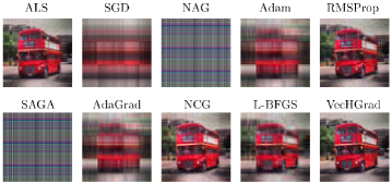
Figure 4: Visual simulation of the accuracy at convergence of the different optimizers for the PARATUCK2 decomposition. The accuracy is highlighted by how blurry the image is (error at convergence ALS: 1018, SGD: 4082, NAG: 6469, Adam: 2996, RMSProp: 1184, SAGA: 6378, AdaGrad: 2961, NCG: 1569, L-BFGS: 1771, VecHGrad: 599). The popular gradient optimizers AdaGrad, NAG and SAGA failed to converge to a solution close to the original image, contrarily to VecHGrad or RMSProp.

In a second experiment, we compared in Table 2 and Table 3 the loss function errors and the calculation times of the optimizers for the five ML data sets described in Table 1 for the three TDs aforementioned. Both the loss function errors and the calculation times were computed based on the mean of the loss function errors and the mean of the calculation times over all batches. The numerical schemes of the NAG, SAGA and AdaGrad algorithms failed to minimize the error of the loss function accurately. The ALS scheme furthermore offers a good compromise between the resulting errors and the required calculation times, explaining its major success across TD applications. The gradient descent optimizers, Adam and RMSProp, and the Hessian based optimizers, VechGrad and L-BFGS, were capable to minimize the loss function the most accurately. The NCG method achieved satisfying errors for the CP and the DEDICOM decomposition but its performance decreases significantly when trying to solve the PARATUCK2 decomposition. Surprisingly, the calculation times of the Adam and RMSProp gradient descents were greater than the calculation times of VecHGrad. VecHGrad was capable to outperform the gradient descent schemes for both accuracy and speed thanks to the use of the strong Wolfe’s line search and the vector Hessian approximation, inherited from gradient information. This result is reported in Table 4 presenting the experimental mean convergence rate, defined such that $q\approx\log\left|\frac{\textbf{f}^{t+1}-\textbf{f}^{t}}{\textbf{f}^{t}-\textbf{f}^{t-1}}\right|\begin{bmatrix}\log\left|\frac{\textbf{f}^{t}-\textbf{f}^{t-1}}{\textbf{f}^{t-1}-\textbf{f}^{t-2}}\right|\end{bmatrix}^{-1}$ for PARATUCK2 TD. The latter underlines the best differences between the optimizers. The highest convergence rate was obtained by VecHGrad, followed by L-BFGS and NCG. Similar values were obtained for the other decomposition. Thus, we can conclude that VecHGrad is capable to solve accurately and efficiently TDs outperforming popular machine learning gradient descent algorithms.

Table 2: Mean of the loss function errors at convergence over all batches. The lower, the better. The strong Wolfe’s line search is crucial for the VecHGrad’s performance.

Decomposition	Optimizer	CIFAR-10	CIFAR-100	MNIST	COCO	LFW
CP	ALS	318.667	428.402	897.766	485.138	4792.605
CP	SGD	2112.904	2825.710	2995.528	3407.415	7599.458
CP	NAG	4338.492	5511.272	4916.003	8187.315	18316.589
CP	Adam	1578.225	2451.217	1631.367	2223.211	6644.167
CP	RMSProp	127.961	128.137	200.002	86.792	4205.520
CP	SAGA	4332.879	5501.528	4342.708	6327.580	13242.181
CP	AdaGrad	3142.583	4072.551	2944.768	4921.861	10652.488
CP	NCG	41.990	37.086	23.320	76.478	4130.942
CP	L-BFGS	195.298	525.279	184.906	596.160	4893.815
CP	VecHGrad	$\leq$ 1.000	$\leq$ 1.000	$\leq$ 1.000	$\leq$ 1.000	$\leq$ 1.000
DEDICOM	ALS	1350.991	1763.718	1830.830	1894.742	3193.685
DEDICOM	SGD	435.780	456.051	567.503	406.760	511.093
DEDICOM	NAG	4349.151	5722.073	4415.687	6325.638	9860.454
DEDICOM	Adam	579.723	673.316	575.341	743.977	541.515
DEDICOM	RMSProp	63.795	236.974	96.240	177.419	33.224
DEDICOM	SAGA	4285.512	5577.981	4214.771	5797.562	8128.724
DEDICOM	AdaGrad	1962.966	2544.436	1452.278	2851.649	3033.965
DEDICOM	NCG	550.554	321.332	171.181	583.430	711.549
DEDICOM	L-BFGS	423.802	561.689	339.284	435.188	511.620
DEDICOM	VecHGrad	$\leq$ 1.000	$\leq$ 1.000	$\leq$ 1.000	$\leq$ 1.000	$\leq$ 1.000
PARATUCK2	ALS	408.724	480.312	1028.250	714.623	658.284
PARATUCK2	SGD	639.556	631.870	1306.869	648.962	495.188
PARATUCK2	NAG	4699.058	6046.024	5168.824	8205.223	14546.438
PARATUCK2	Adam	512.725	680.653	591.156	594.687	615.731
PARATUCK2	RMSProp	133.416	145.766	164.709	134.047	174.769
PARATUCK2	SAGA	4665.435	5923.178	4934.328	6350.172	8847.886
PARATUCK2	AdaGrad	1775.433	2310.402	1715.316	2752.348	2986.919
PARATUCK2	NCG	772.634	1013.032	270.288	335.532	15181.961
PARATUCK2	L-BFGS	409.666	522.158	464.259	467.139	416.761
PARATUCK2	VecHGrad	$\leq$ 1.000	$\leq$ 1.000	$\leq$ 1.000	$\leq$ 1.000	$\leq$ 1.000

Table 3: Mean calculation times (sec.) to reach convergence over all batches.

Decomposition	Optimizer	CIFAR-10	CIFAR-100	MNIST	COCO	LFW
CP	ALS	5.289	4.584	2.710	5.850	4.085
CP	SGD	1060.455	1019.432	0.193	2335.060	6657.985
CP	NAG	280.432	256.196	0.400	1860.660	1.317
CP	Adam	2587.467	2771.068	2062.562	6667.673	6397.708
CP	RMSProp	2013.424	2620.088	2082.481	5588.660	4975.279
CP	SAGA	1141.374	1160.775	0.191	3504.593	3692.471
CP	AdaGrad	1768.562	2324.147	959.408	3729.306	6269.536
CP	NCG	315.132	165.983	4.910	778.279	716.355
CP	L-BFGS	2389.839	2762.555	2326.405	5936.053	5494.634
CP	VecHGrad	200.417	583.117	644.445	1128.358	1866.799
DEDICOM	ALS	21.280	70.820	14.469	55.783	158.946
DEDICOM	SGD	1826.214	1751.355	1758.625	1775.100	1145.594
DEDICOM	NAG	30.847	25.820	240.587	43.003	49.518
DEDICOM	Adam	2105.825	2128.626	1791.295	2056.036	1992.987
DEDICOM	RMSProp	1233.237	1129.172	993.429	1140.844	1027.007
DEDICOM	SAGA	27.859	30.970	64.440	28.319	32.154
DEDICOM	AdaGrad	196.208	266.057	1856.267	2020.417	2027.370
DEDICOM	NCG	2524.762	644.067	236.868	1665.704	4219.446
DEDICOM	L-BFGS	1568.677	1519.808	1209.971	1857.267	1364.027
DEDICOM	VecHGrad	592.688	918.439	412.623	607.254	854.839
PARATUCK2	ALS	225.952	209.978	230.392	589.437	625.668
PARATUCK2	SGD	1953.609	2625.722	2067.727	3002.172	2745.380
PARATUCK2	NAG	48.468	48.724	285.679	76.811	72.068
PARATUCK2	Adam	2628.211	2657.387	2081.996	2719.519	2709.638
PARATUCK2	RMSProp	1407.752	1156.370	1092.156	1352.057	1042.899
PARATUCK2	SAGA	74.248	70.952	120.861	71.398	86.682
PARATUCK2	AdaGrad	2595.478	2626.939	2073.777	292.564	2795.260
PARATUCK2	NCG	150.196	1390.013	928.071	1586.523	82.701
PARATUCK2	L-BFGS	2780.658	2656.062	2188.253	3522.249	2822.661
PARATUCK2	VecHGrad	885.246	1149.594	1241.425	1075.570	1222.827

Table 4: PARATUCK2 experimental mean convergence rate per step.

ALS	SGD	NAG	Adam	RMSProp	SAGA	AdaGrad	NCG	L-BFGS	VecHGrad
0.958	1.004	1.010	1.009	0.992	0.994	0.983	1.376	1.452	1.551

6 Conclusion

We introduced VecHGrad, a Vector Hessian Gradient optimization method, to solve accurately linear algebra error minimization problems. VecHGrad uses a strong Wolfe’s line search, crucial for fast convergence and accurate resolution, with partial information of the second derivative. We conducted experiments on five real data sets, CIFAR10, CIFAR100, MNIST, COCO and LFW, very popular in machine learning and deep learning. We highlighted that VecHGrad is capable to outperform widely-used gradient-based resolution methods, such as Adam, RMSProp or Adagrad, on three different tensor decompositions, CP, DEDICOM and PARATUCK2, offering different levels of linear algebra complexity. We emphasized our experiments with machine learning optimizers since VecHGrad can be easily applied to solve machine learning error minimization problems. Surprisingly, the runtimes of the gradient-based and the Hessian-based optimization methods were very similar as the runtime per step of the gradient-based methods was slightly faster, but their convergence per step was lower. Therefore, gradient-based optimization methods require more iterations to converge. Furthermore, the accuracy of some of the popular schemes, such as NAG, was fairly poor while requiring a similar runtime than that of the other methods. Future work will concentrate on the influence of the adaptive line search to other machine learning optimizers. We observed that the performance of the algorithms is strongly correlated to the performance of the the adaptive line search optimization. Simultaneously, we will look to reduce the memory cost of the adaptive line search as it has a crucial impact on a GPU implementation. We will finally provide a Python and PyTorch public implementations of our method to answer the need of the machine learning and deep learning communities.

References

- [1] Globerson, A., Chechik, G., Pereira, F., Tishby, N.: Euclidean embedding of co-occurrence data. Journal of Machine Learning Research (2007)
- [2] Zhou, S., Erfani, S.M., Bailey, J.: Online cp decomposition for sparse tensors (2018)
- [3] Kolda, T.G., Bader, B.W.: Tensor decompositions and applications. SIAM review (2009)
- [4] Carroll, J.D., Chang, J.J.: Analysis of individual differences in multidimensional scaling via an N-way generalization of “Eckart-Young” decomposition. Psychometrika (1970)
- [5] Harshman, R.A.: Foundations of the parafac procedure: Models and conditions for an explanatory multimodal factor analysis (1970)
- [6] Bader, B.W., Harshman, R.A., Kolda, T.G.: Temporal analysis of semantic graphs using asalsan. In: ICDM. IEEE (2007)
- [7] Harshman, R.A., Lundy, M.E.: Uniqueness proof for a family of models sharing features of tucker’s three-mode factor analysis and PARAFAC/CANDECOMP. Psychometrika (1996)
- [8] Charlier, J.H.J., Falk, E., Hilger, J., et al.: User-device authentication in mobile banking using APHEN for PARATUCK2 tensor decomposition. In: ICDMW. IEEE (2018)
- [9] Robbins, H., Monro, S.: A stochastic approximation method, annals math. Statistics (1951)
- [10] Kiefer, J., Wolfowitz, J., et al.: Stochastic estimation of the maximum of a regression function. The Annals of Mathematical Statistics (1952)
- [11] Wright, S., Nocedal, J.: Numerical optimization. Springer Science (1999)
- [12] Duchi, J., Hazan, E., Singer, Y.: Adaptive subgradient methods for online learning and stochastic optimization. Journal of Machine Learning Research (2011)
- [13] Kingma, D.P., Ba, J.: Adam: A method for stochastic optimization. arXiv preprint arXiv:1412.6980 (2014)
- [14] Nesterov, Y., et al.: Gradient methods for minimizing composite objective function (2007)
- [15] Defazio, A., Bach, F., Lacoste-Julien, S.: SAGA: A fast incremental gradient method with support for non-strongly convex composite objectives. In: Advances in neural information processing systems (2014)
- [16] Gupta, V., Koren, T., Singer, Y.: Shampoo: Preconditioned stochastic tensor optimization. arXiv preprint arXiv:1802.09568 (2018)
- [17] Acar, E., Dunlavy, D.M., Kolda, T.G.: A scalable optimization approach for fitting canonical tensor decompositions. Journal of Chemometrics (2011)
- [18] Hinton, G., Srivastava, N., Swersky, K.: Rmsprop: Divide the gradient by a running average of its recent magnitude. Neural networks for machine learning, Coursera lecture 6e (2012)
- [19] Harshman, R.A.: Models for analysis of asymmetrical relationships among n objects or stimuli. In: First Joint Meeting of the Psychometric Society and the Society of Mathematical Psychology, Hamilton, Ontario (1978)
- [20] Bro, R.: Multi-way analysis in the food industry: models, algorithms, and applications. Ph.D. thesis, Københavns UniversitetKøbenhavns Universitet (1998)
- [21] Charlier, J., Hilger, J., et al.: Non-negative paratuck2 tensor decomposition combined to LSTM network for smart contracts profiling. In: BigComp. IEEE (2018)
- [22] Acar, E., Kolda, T.G., Dunlavy, D.M.: All-at-once optimization for coupled matrix and tensor factorizations. arXiv preprint arXiv:1105.3422 (2011)
- [23] Maehara, T., Hayashi, K., Kawarabayashi, K.i.: Expected tensor decomposition with stochastic gradient descent. In: AAAI. pp. 1919–1925 (2016)
- [24] Schittkowski, K.: NLPQLP: A new Fortran implementation of a sequential quadratic programming algorithm for parallel computing. Report, Department of Mathematics, University of Bayreuth (2001)
- [25] Liu, D.C., Nocedal, J.: On the limited memory BFGS method for large scale optimization. Mathematical programming (1989)