Transverse optical pumping of spin states

Abstract

Optical pumping is an efficient method for initializing and maintaining atomic spin ensembles in a well-defined quantum spin state. Standard optical-pumping methods orient the spins by transferring photonic angular momentum to spin polarization. Generally the spins are oriented along the propagation direction of the light due to selection rules of the dipole interaction. Here we present and experimentally demonstrate that by modulating the light polarization, angular momentum perpendicular to the optical axis can be transferred efficiently to cesium vapor. The transverse pumping scheme employs transversely oriented dark states, allowing for control of the trajectory of the spins on the Bloch sphere. This new mechanism is suitable and potentially beneficial for diverse applications, particularly in quantum metrology.

Optical pumping is the prevailing technique for orienting atomic spins, conveying order from polarized light onto the state of spins (Happer-1972, ; Happer-book, ; Auzinsh-book, ). Many applications in precision metrology (Budker-Romalis-optical-magnetometery, ; Serf-magnetometer, ; Kitching-sensors, ; Treutlein-microwave-imaging, ), quantum information (Polzik-RMP-2010, ; POlzik2017, ; Novikova-review, ), noble gas hyper-polarization (happer-walker-rmp, ; happer-1998, ; Chupp, ), and searches for new physics beyond the standard model (fundamental-physics, ; romalis-fundamental-physics, ) employ optical pumping for initializing the orientation moment of the spins, that is, for pointing the spins towards a preferred direction. The required degree of polarization depends on the specific application, where optimized performance in quantum metrology is often practically achieved around 50% polarization (romalis-hybrid, ; fifty_precent_polarization, ; Muschik, ). Standard optical pumping schemes generate polarization along the propagation direction of the laser beam. These schemes include depopulation pumping (Happer-1972, ), synchronous pumping (Weis-PM-1, ; Romalis-2007, ; SYNCHRONEOUS-PUMPING2, ), spin-exchange indirect pumping (Chalupczak-indirect-SE-pumping, ; Chalupczak-spin-maser, ), alignment-to-orientation conversion (Budker-AOC, ), and hybrid spin-exchange pumping (romalis-hybrid, ). However in various applications, it is often desired to polarize the spins along an applied magnetic field, perpendicular to the optical axis (Muschik, ; Budker-book, ; kitching-pump-probe, ; Walker-NMRG, ; SERF-storage-of-light, ). While at extreme magnetic fields, it is possible to polarize the spins transversely (footnote1, ), at moderate magnetic fields, typical to alkali-metal spins experiments for example, the pumping efficiency is rather low.

Here we propose and demonstrate an optical pumping scheme for efficient spin polarization transversely to the propagation direction of the laser beam. The scheme incorporates a polarization-modulated light beam, which steers the spins in helical-like trajectories on the Bloch sphere around and along a transverse magnetic field, while gradually increasing their polarization. The scheme exhibits sharp resonances, reaching maximum efficiency when the optical modulation is resonant with the Larmor precession of the spins. We develop a simple analytical model for analyzing the experimental results and discuss the applicability of the scheme for various applications.

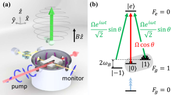
Figure 1: Experimental system and toy model. (a) Schematics of the experimental setup and the spiral motion of the atomic spins (green) towards $+\hat{z}$. The polarization of the pump beam (red) alternates between linear and circular (blue arrows). The spin orientation is monitored using balanced polarimetry of a far-detuned monitor beam (yellow). Not shown are the repump beam and a second monitor beam, which co-propagate with the pump. (b) Toy model with $I=1/2$. The repump laser (blue arrow) empties the $F_{g}=0$ state, while the pump laser (red and green arrows) drives the atoms into the dark state $|d_{+}\rangle\propto\cos\theta\left|1\right\rangle-\tfrac{1}{\sqrt{2}}e^{i\omega t}\sin\theta\left|0\right\rangle$ (gray shading), eventually oriented perpendicular to the beam direction.

In standard optical pumping schemes, the atomic ground state is polarized via repeated cycles of absorption and spontaneous emission. Ideally, the atoms cease to absorb the pump photons when they reach a ‘dark state’, which is determined by the excited transitions during pumping (Happer-1972, ). For a light field with an electric field $\mathbf{E}\left(t\right)=E_{0}e^{i(\omega_{\mathrm{L}}t-kx)}\hat{e}$, the relevant transitions depend on the relative detuning of the light frequency $\omega_{\mathrm{L}}$ from the atomic transition frequency $\omega_{0}$, on the external electric and magnetic fields, and on the selection rules of the dipole interaction for polarization $\hat{e}$. For alkali-metal vapors, the latter dominates the pumping process of spin orientation at moderate magnetic fields, because the ground and excited magnetic sublevels $|F_{g},m_{g}\rangle,\,|F_{e},m_{e}\rangle$ within each hyperfine manifold $F_{g},\,F_{e}$ are optically unresolved.

For constant polarization $\hat{e}$, one-photon absorption of light does not produce a considerable spin orientation transversely to the optical axis. Circular light polarization $\hat{e}_{\pm}=(\hat{y}\pm i\hat{z})/\sqrt{2}$ orients the spins along the optical axis $\pm\hat{x}$ via the allowed transitions $m_{e}=m_{g}\pm 1$; For $F_{e}\leq F_{g}$, the maximally polarized state $|m_{g}=\pm F_{g}\rangle$ is dark. Linearly polarized light $\hat{e}=\hat{y},\hat{z}$ generates spin alignment along $\hat{x}\times\hat{e}$ and zero net orientation with the selection rules $m_{e}=m_{g}$ when tuned to the transition $F_{g}\rightarrow F_{e}=F_{g}-1$; This generates a quadrupole magnetic moment (Happer-1972, ), leaving both $|m_{g}=F_{g}\rangle$ and $|m_{g}=-F_{g}\rangle$ dark. It thus seems that no orientation is built perpendicularly to the optical axis $\hat{x}$ for any light polarization. Our scheme overcomes this limitation and allows for transverse optical pumping of the spins by temporally modulating the light polarization.

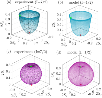
Figure 2: Spin trajectories on the Bloch sphere. The optical axis is $\hat{x}$, within the equatorial plane. (a,c) Measurements of the pumping process from $t=0$ to $t=100$ ms. (b,d) Theoretical toy model with $I=1/2$. Red (green) circles mark the initial (final) states of the spin. (a) When pumping with a constant modulation depth $\theta=0.2\;\mbox{rad}$, the measured cesium spins follow a spiral-helical trajectory around the $+\hat{z}$ direction. (c) Adiabatically varying $\theta\left(t\right)$ allows for driving the spins in a spherical-helical trajectory that ends along the $\hat{z}$ axis.

Results

We employ the experimental setup shown schematically in Fig. 1(a), containing cesium vapor at room temperature. Setting a constant magnetic field $B\hat{z}$ determines the quantization axis $\hat{z}$ and the Larmor frequency $\omega_{\mathrm{B}}=gB$, where $g=0.35\,(2\pi)\text{MHz/G}$ is the gyro-magnetic ratio for cesium. For the transverse pumping, we use a pump beam, which frequency is tuned to the $D_{1}$ transition $F_{g}=4\rightarrow F_{e}=3$ and which polarization is modulated according to

$$\hat{e}\left(t\right)=\cos\left(\theta\right)\hat{z}+ie^{i\omega t}\sin\left(\theta\right)\hat{y}.$$ (1)

Here $\sin\left(\theta\right)$ is the modulation depth and $\omega$ is the modulation angular frequency. For the sake of analysis and presentation, we introduce two far-detuned monitor beams propagating along $\hat{x}$ and $\hat{y}$, measuring the three dimensional orientation state of the spins $(2S_{x},2S_{y},2S_{z})$ on the Bloch sphere during the pumping process. See Methods for additional experimental details.

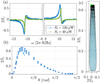
Figure 3: Pumping dependence on the modulation parameters. (a) Measured $S_{z}\left(\omega\right)$ at $t=200\;\mbox{msec}$ for cesium atoms with $\theta=0.24\;\mbox{rad}$ and $\omega_{\mathrm{B}}=10.2\;\mbox{(2$\pi$)kHz}$. The resonance peaks at $\omega\approx\pm\omega_{\mathrm{B}}$ are associated with the two CPT dark states $|d_{\pm}\rangle$. (b) Dependence on the modulation depth $\theta$: measured $S_{z}\left(\theta\right)$ at $t=200\;\mbox{msec}$ with $\omega=\pm 10.3\;(2\pi)\text{kHz}$ and $P_{0}=120\;\mbox{$\mu$W}$. Pumping is optimal at moderate modulation depths, such that $|d_{+}\rangle$ is oriented towards $+\hat{z}$, but $\Gamma\sin^{2}\left(\theta\right)\apprge\gamma$. (c) Measured spin trajectory, corresponding to the point point marked by an arrow in b. The final polarization (green circle) is along $\hat{z}$, i.e. perpendicular to the optical axis, with a small residual polarization along $\hat{x}$ and $\hat{y}$.

A typical measurement during the pumping process is presented on the Bloch sphere in Fig. 2(a). We observe that the spin orientation follows a helical trajectory transversely to the optical axis $\hat{x}$. In this experiment, the pump power is $P_{0}=250\;\mbox{$\mu$W}$ and the modulation frequency is tuned to resonate with the Larmor frequency $\omega_{\mathrm{B}}\approx\omega=1.5\;(2\pi)\mbox{kHz}$. The final value of $2S_{z}$ quantifies the pumping efficiency. Its dependence on the modulation parameters $\omega$ and $\theta$ is shown in Fig. 3. We identify two resonant features of $2S_{z}\left(\omega\right)$ at $\omega\approx\pm\omega_{\mathrm{B}}$ as shown in Fig. 3(a) for $\theta=0.24$ and two laser powers. The laser power governs the width of the resonance as well as the shift of the peak from the actual Larmor frequency. Figure 3(b) presents $2S_{z}\left(\theta\right)$ on one of the resonances $[\omega=10.3\;(2\pi)\mbox{KHz]}$. We achieved an overall maximal polarization of $2S_{z}=65\%$ (with small residual transverse polarization $2$$\sqrt{S_{x}^{2}+S_{y}^{2}}$$=3.5\%$) as shown in Fig. 3(c).

To explain the transverse pumping mechanism we utilize a simple model of an alkali-like level structure with nuclear spin $I=1/2$, as shown in Fig. 1(b). The magnetic field $\mathbf{B}=B\hat{z}$ (henceforth assume $B>0$) breaks the isotropy in the transverse $yz$ plane, setting our quantization axis $\hat{z}$ and splitting the Zeeman sublevels $\left|0\right\rangle,\left|\pm 1\right\rangle$ by $\hbar\omega_{\mathrm{B}}$. The $F_{g}=0$ level is emptied by a repump field or by spin-exchange collisions. The pump field, resonant with the $F_{g}=1\rightarrow F_{e}=0$ transition, is polarization-modulated according to Eq. (1). We describe the effect of the polarization modulation on the spins dynamics by decomposing the polarization vector $\hat{e}\left(t\right)$ into its Stokes components $\boldsymbol{\hat{s}}=(s_{1},s_{2},s_{3})$ (Romalis-Dead-Zone-Free-magnetometer, ). The unmodulated linear polarization $\hat{z}$, represented by $s_{1}$, aligns the atoms along $\hat{z}$ at a rate $R_{a}\sim\Gamma\cos^{2}\left(\theta\right)$, creating spin-alignment (see Supplementary Note). Here $\Gamma=\Omega^{2}/\gamma_{\mathrm{e}}$ is the characteristic pumping rate, with $\gamma_{\mathrm{e}}$ the spontaneous emission rate and $\Omega$ the Rabi frequency of the pump beam. The linear polarization $(\hat{y}\pm\hat{z})/\sqrt{2}$, represented by $s_{2}$, induces a tensor light shift of $\Gamma\sin\left(2\theta\right)\sin\left(\omega t\right)$ along $\pm\hat{x}$, which acts like a magnetic field. The circular polarization $\hat{e}_{\pm}$, represented by $s_{3}$, pumps the spins longitudinally along $\pm\hat{x}$ at a rate $\Gamma\sin\left(2\theta\right)\cos\left(\omega t\right)$. Therefore, the modulated polarization alternates between pumping ($s_{3}$) and light-shifting ($s_{2}$) the atomic spins along $\hat{x}$ at a rate $\omega$. For $\omega=\omega_{\mathrm{B}}$, the pumping and light shifts are synchronous, efficiently driving the precessing spins away from the $xy$ plane, transversely to the optical axis. The resulting evolution of the Bloch vector $(2S_{x},2S_{y},2S_{z})$ is shown graphically in Fig. 4 and further detailed in Methods.

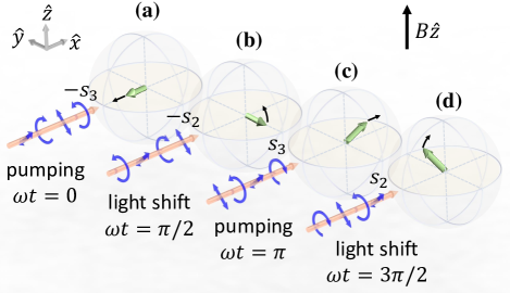
Figure 4: Transverse pumping mechanism. One period of the transverse pumping mechanism for synchronous modulation $\omega=\omega_{\mathrm{B}}$. The spins (green arrows) precess $\omega_{\mathrm{B}}t=\pi/2$ radians between each subplot due to the magnetic field $B\hat{z}$. (a) The spins are optically-pumped towards $-\hat{x}$. (b+d) The spins are tilted towards $+\hat{z}$ due to tensor light-shift. (c) The spins are optically-pumped towards $+\hat{x}$. Black arrows indicate the pumping/tilting directions. The eventual spin orientation is along $+\hat{z}$, perpendicular to the propagation direction of the pumping beam.

The toy model enables to reconstruct the main features of the measured trajectories as shown in Fig. 2(b), by solving the $I=1/2$ model numerically and tuning its parameters (see Supplementary Note). We note however that this model only aims at explaining the qualitative features of the process, while disregarding effects arising from the multilevel structure of cesium, which may reduce the pumping efficiency.

The resonant nature of the pumping process can also be understood as originating from coherent population trapping (CPT) (Fleischhauer-EIT-RMP, ). In CPT, a dark state is formed within a $\Lambda$ level-system via destructive interference of two excitation pathways. Considering the level structure in Fig. 1(b) and decomposing the modulated pump into its two polarization components $E\hat{z}$ and $E\hat{y}$, we identify two $\Lambda$ systems: $\Lambda_{+}=\{\left|1\right\rangle,\left|e\right\rangle,\left|0\right\rangle\}$ and $\Lambda_{-}=\{\left|-1\right\rangle,\left|e\right\rangle,\left|0\right\rangle\}$. System $\Lambda_{+}$ has the dark state $|d_{+}\rangle\propto\cos\left(\theta\right)\left|1\right\rangle-\tfrac{1}{\sqrt{2}}e^{i\omega t}\sin\left(\theta\right)\left|0\right\rangle$ at $\omega\approx\omega_{\mathrm{B}}$, while system $\Lambda_{-}$ has the dark state $|d_{-}\rangle\propto\cos\left(\theta\right)\left|-1\right\rangle-\tfrac{1}{\sqrt{2}}e^{i\omega t}\sin\left(\theta\right)\left|0\right\rangle$ at $\omega\approx-\omega_{\mathrm{B}}$. For $\theta\ll 1$, the dark states $|d_{\pm}\rangle\approx\left|\pm 1\right\rangle$ represent the polarized states perpendicular to the optical axis. The application of magnetic field $B\hat{z}$ separates the CPT resonances of $\Lambda_{+}$ and $\Lambda_{-}$ by $2\omega_{\mathrm{B}}$, so that the states $|d_{+}\rangle$ and $|d_{-}\rangle$ cannot be simultaneously dark when $\omega_{\mathrm{B}}\gg\Gamma$. Consequently, setting $\omega=\omega_{\mathrm{B}}$ depopulates the $\Lambda_{-}$ system while pumping the $\Lambda_{+}$ system towards the transversely oriented dark state $|d_{+}\rangle$. We conclude that destructive interference of two excitation pathways effectively modifies the absorption selection-rules, such that one polarized state (e.g. $\left|-1\right\rangle$ for $\omega_{\mathrm{B}}>0$) absorbs photons, while the opposite state ($\left|1\right\rangle$ for $\omega_{\mathrm{B}}>0$) is transparent.

We associate the two resonances in Fig. 3(a) with the CPT dark states of $\Lambda_{+}$ at $\omega>0$ and $\Lambda_{-}$ at $\omega<0$. In the absence of the upper hyperfine level $F_{e}=4$, the resonances would have seen like single peaks; it is the presence of $F_{e}=4$ that introduces the second peaks (with opposite sign) in each resonance, as well as the shift of the peak from $\omega=\omega_{\mathrm{B}}$ and the asymmetry between positive and negative $\omega$. As seen in Fig. 3(b), the pumping is most efficient at moderate modulation depths: For $\theta\rightarrow\pi/2$ the dark state is $|d_{+}\rangle\rightarrow\left|0\right\rangle$, with zero net orientation. For $\theta\rightarrow 0$, the dark state is $|d_{+}\rangle\approx\left|1\right\rangle$, but the depopulating rate of $|d_{-}\rangle$, proportional to $\Gamma\sin^{2}\left(\theta\right)$, is too small compared to the overall depolarization rate $\gamma$.

A benefit of the CPT resonant operation is the ability to temporally vary the system state in a controlled, adiabatic manner. To demonstrate this, we monitor the pumping process on resonance [$\omega=\omega_{\mathrm{B}}=1.5\;(2\pi)\mbox{KHz}$], while temporally varying $\theta$ over a duration $T=100\;\mbox{msec}$ according to $\theta\left(t\right)=\arccos\sqrt{t/T}$. The spin state, initially pumped to $|d_{+}\rangle{}_{\theta\left(t=0\right)}\approx\left|0\right\rangle$, adiabatically follows the varying dark-state $|d_{+}\rangle{}_{\theta\left(t\right)}$ to its final value $|d_{+}\rangle{}_{\theta\left(t=T\right)}\approx\left|1\right\rangle$, tracing a spherical-like trajectory as shown in Fig. 2(c) (experiment) and Fig. 2(d) (theory). This process is similar to stimulated Raman adiabatic passage (stirap, ) and can therefore be used to tailor desired trajectories and final states. Notably it enables the zeroing of the transverse spin components $S_{x}$ and $S_{y}$ at the end of the process, as shown in Figs. 2(c,d).

Discussion

It is relatively simple to implement the presented scheme in applications. Polarization modulation can be done using a single photo-elastic modulator (Hinds, ) or with readily available, on chip, integrated photonics (Op5tical-chip, ). Various applications that rely on optical spin manipulation would potentially benefit from utilizing the scheme. Here we briefly consider some directions with spin vapors.

First, devices currently employing perpendicular beams in a pump-probe configuration (Budker-book, ; kitching-pump-probe, ; Walker-NMRG, ) could be realized with a simpler, co-propagating arrangement, with the spins oriented transversely to the optical axis. Such arrangement is most beneficial for miniaturized sensors, such as NMR-oscillators (Walker-NMRG, ), where the size and complexity depend crucially on the beams configuration, especially if the light source, manipulation, and detection can be implemented on a single stack over a chip (kitching-pump-probe, ). These sensors are used in various applications as well as in fundamental research, such as search for new physics (WALKER-pt-ciolation-nmrg, ; budker-optical-magnetometer, ). Particularly for NMR-oscillators, the projection of the alkali spin along the magnetic field will be unmodulated, thus sustaining the spin-exchange optical-pumping of the noble gas spins.

Second, any application that is restricted to a single laser direction can now use our scheme to control and fine tune the final direction of the pumped spins (longitudinal, transversal, or combination thereof). Such applications include remote magnetometry of mesospheric sodium spins (Budker-book, ; budker-mesospheric, ), steady-state entanglement generation during pumping (Muschik, ), optical pumping of metastable ${}^{3}\text{He}$ for medical imaging (Walker-He3, ), and coherent manipulation of the internal spin state of cold atoms without associate heating (Footnote3, ).

Third, transverse pumping may form the basis for an all-optical magnetometer using either alkali-metal atoms or metastable ${}^{4}\text{He}$ atoms designed for space applications (Budker-book, ; budker-optical-magnetometer, ). This magnetometer would rely on measuring the resonant response to the modulated light, providing a dead-zone-free operation (Romalis-Dead-Zone-Free-magnetometer, ), or on measuring the Faraday-rotation of off-resonant probe light, thus reducing the photon shot-noise commonly limiting magnetometers based on electromagnetically induced transparency (Fleischhauer-EIT-magnetometer-limit, ). Moreover, the polarization-modulated pump generates the $m=1$ Zeeman coherence (SERF-storage-of-light, ), implying that these magnetometers could operate in the spin-exchange relaxation-free (SERF) regime (nonlinear-SERF, ).

Finally, our scheme does not rely on any process particular to vapor physics. It is thus readily application to any spin system having a non-degenerate Λ-system with a meta-stable ground manifold, such as those employed in diamond color centers (nv_CENTERS, ; nv-center2, ), rare-earth doped crystals (RARE-EARTH, ), and semiconductor quantum dots (QDot, ; QDot2, ; SIV-Nunn, ).

In conclusion, we have demonstrated a new optical pumping technique, generating significant spin orientation transversely to the propagation direction of the pump beam. The spins are oriented along the external transverse magnetic field via alternating actions of pumping and tensor light-shifts, which are resonant with the Larmor precession. The resonance features, associated with transversely orientated dark-states, allow one to control the spin trajectory on the Bloch sphere by varying the modulation parameters. This scheme could be highly suitable for quantum-metrology applications.

Methods

Additional experimental details:

We use a $10$-mm diameter, $30$-mm long cylindrical glass cell containing cesium vapor ($I=7/2,\,S=1/2$) at room temperature. The cell is paraffin coated and free of buffer gas, exhibiting spin coherence time of 150 ms (SERF-storage-of-light, ). We set a constant magnetic field $B\hat{z}$ in the cell using Helmholtz coils and four layers of magnetic shields. For the transverse pumping, we use an $895\;\mbox{nm}$ single-mode pump beam. We modulate the pump polarization by splitting it with a polarizing beam splitter (PBS) and sending each output arm to an acousto-optic modulator. The beams deflected by the modulators are recombined and mode-matched using a second PBS, resulting with the polarization given in Eq. 1. The laser frequency after passing the modulators is tuned to the $D_{1}$ transition $F_{g}=4\rightarrow F_{e}=3$. We control the modulation depth $\sin\left(\theta\right)$ by rotating the linear polarization before the first PBS and control the modulation angular frequency $\omega$ by setting the relative RF frequencies of the two modulators. To keep the lower hyperfine manifold $F_{g}=3$ empty, we use 1 mW of auxiliary repump beam at $895\;\mbox{nm}$, resonant with the $F_{g}=3\rightarrow F_{e}=4$ transition and linearly polarized along $\hat{y}$. The pump and repump, both with a diameter of 8 mm, co-propagate along $\hat{x}$.

Reconstruction of the spin state on the Bloch sphere:

The spin state is reconstructed by evaluating the electronic spin orientations $(2S_{x},2S_{y},2S_{z})=\left\langle\mathbf{F}\right\rangle/4$, where $\left\langle\mathbf{F}\right\rangle$ is the orientation moment of the total spin operator $\mathbf{F}=\mathbf{I+S}$. The spin orientations are measured by using balanced polarimetry of two linearly-polarized far-detuned monitor beams propagating along $\hat{x}$ and $\hat{y}$. At low atomic densities and depopulated $F_{g}=3$ hyperfine manifold, the detected Faraday-rotation angles are proportional to the spin orientation along the direction of the beam (Happer-book, ; coherent-coupling, ). We calibrate the proportionality constants of each monitor beam by measuring its maximal polarization rotation when the ground state is fully pumped using two circularly-polarized beams resonant with the two ground-state hyperfine manifolds. We reconstruct the three spin components by making two consecutive measurements: First, $S_{x}$ and $S_{y}$ are measured when $\mathbf{B}=B\hat{z}$. Second, a measurement is conducted with $\mathbf{B}=B\hat{y}$ and $\theta$ changed by $\theta\rightarrow\pi/2-\theta$, keeping the other experimental parameters unchanged. As a result, spin is built along $\hat{y}$ and measured by the $\hat{y}$ monitor. This provides the $S_{z}$ component of the first configuration. We verify that $S_{x}$ is unaffected by the change of $\theta,B$, by that confirming that the parameter change is appropriate.

Spin dynamics with polarization-modulated light:

For small modulation depths $\theta\ll 1$, the dynamics is governed by Bloch-like equations of the vector $\left\langle\mathbf{F}\right\rangle=(F_{x},F_{y},F_{z})$ (see Supplementary Note for the general treatment). The spin orientations $F_{x}$ (along the optical axis) and $F_{y}$ are subject to

$$\dot{F}_{x} = -\gamma_{\perp}F_{x}-\omega_{\mathrm{B}}F_{y}-\Gamma\sin\left(2\theta\right)\cos\left(\omega t\right),$$ (2)

$$\dot{F}_{y} = -\gamma_{\perp}F_{y}+\omega_{\mathrm{B}}F_{x}+\Gamma\sin\left(2\theta\right)\sin\left(\omega t\right)F_{z},$$ (3)

which include a transverse decay rate $\gamma_{\perp}=\gamma+2\Gamma\cos^{2}\theta$ and Larmor precession at the rate $\omega_{\mathrm{B}}$. Here $\gamma$ denotes a slow ground-state depolarization rate (e.g., due to wall collisions). The third term in Eq. (2) is due to $s_{3}$. It describes a temporally-modulated optical pumping, which is maximal at $\omega t=0$ (and at all $\omega t=2\pi n$ for any integer $n$) towards $-\hat{x}$ (Fig. 4a) and at $\omega t=\pi$ towards $+\hat{x}$ (Fig. 4c). The pumping of $F_{x}$ is thus most efficient when the optical modulation is synchronous with the Larmor precession $\omega=\omega_{\mathrm{B}}$. The third term in Eq. (3) is due to the modulated linear polarization component $s_{2}$. It describes a tensor light-shift, which acts as a magnetic field along $\hat{x}$ that rotates the spins in the $yz$ plane at a modulated rate $\Gamma\sin\left(2\theta\right)\sin\left(\omega t\right)$. The orientation $F_{z}$ along the magnetic field, which we aim to generate, is subject to

$$\dot{F}_{z}=-\gamma_{\parallel}F_{z}-\Gamma\sin\left(2\theta\right)\left[\sin\left(\omega t\right)F_{y}-\cos\left(\omega t\right)\left\{F_{z},F_{x}\right\}\right],$$ (4)

where the first term is a longitudinal decay at a rate $\gamma_{\parallel}=\gamma+2\Gamma\sin^{2}\theta$, the second term is again light shift due to $s_{2}$, and the third term is an alignment-induced shift. The temporal modulation $\sin\left(\omega t\right)$ of the light shift is a key ingredient in pumping $\mathbf{F}$ towards $+\hat{z}$, as it breaks the symmetry between the $\pm\hat{z}$ directions: The sign of the light shift changes together with the sign of $F_{y}$, thus acting as an alternating magnetic field that always tilts the spins towards $+\hat{z}$, with maximal tilting rate obtained at $\omega t=\pi/2$ (Fig. 4b) and $\omega t=3\pi/2$ (Fig. 4d). The tensor term $\{F_{z},F_{x}\}\equiv\bigl{\langle}\left\{\mathbf{F}\hat{z},\mathbf{F}\hat{x}\right\}\bigr{\rangle}$ contributes similar spin buildup in amplitude but with a $\pi/2$ delay (see Supplementary Note). For $\omega=\omega_{\mathrm{B}}$, both the synchronous pumping and the light shift are most efficient, driving the precessing spins away from the $xy$ plane, transversely to the optical axis.

Supplementary Information

In this supplementary material, we derive the Bloch equations [Eqs. (2-4) in the main text] of $I=1/2$ spins interacting with polarization-modulated light. The dynamics of the atoms can be described by the open quantum system Liouville equation

$$\frac{d\rho}{dt}=-i\left[\mathcal{H}_{0},\rho\right]+\underset{\text{SE}}{\underbrace{\gamma_{\mathrm{e}}\sum_{i=-1}^{1}\mathcal{L}\left(\left|i\right\rangle\left\langle e\right|,\rho\right)}}+\underset{\text{SD}}{\underbrace{\gamma\sum_{i=-1}^{1}\mathcal{L}\left(S_{i},\rho\right)}},$$ (S1)

where $\rho$ is the density matrix of a single spin, and $\mathcal{L}$ is the Lindblad super-operator given by

$$\mathcal{L}\left(A,\rho\right)=A\rho A^{\dagger}-\left(A^{\dagger}A\rho+\rho A^{\dagger}A\right)/2.$$

The first term in Eq. (S1) denotes the free Hamiltonian evolution; The second term denotes the excited state decay due to spontaneous emission (SE) at a rate $\gamma_{\mathrm{e}}$; and the last term denotes the ground-state relaxation due to spin destruction (SD) at a rate $\gamma$, caused by interaction of the electronic spin operator $\boldsymbol{S}$ with some thermal bath. The free Hamiltonian term $\mathcal{H}_{0}$ describes the interaction with external magnetic fields and laser beams. It is given by

$$\mathcal{H}_{0} =\omega_{0}\left|e\right\rangle\left\langle e\right|+\omega_{\mathrm{B}}\left(\left|1\right\rangle\left\langle 1\right|-\left|-1\right\rangle\left\langle-1\right|\right)$$ (S2)

$$+ \Omega\bigl{[}\cos\left(\theta\right)e^{i\omega_{L}t}\left|0\right\rangle\left\langle e\right|+(1/\sqrt{2})\sin\left(\theta\right)e^{i\left(\omega_{L}+\omega\right)t}\left(\left|-1\right\rangle\left\langle e\right|+\left|1\right\rangle\left\langle e\right|\right)+\text{H.c.}\bigr{]},$$

where $\omega_{0}$ is the optical transition to the excited state, $\omega_{\mathrm{B}}=gB/(2\hbar)$ is the Larmor frequency induced by the magnetic field $B\hat{z}$, $\omega_{L}$ is the laser oscillation rate, $\omega$ is the polarization-modulation rate and $\sin\left(\theta\right)$ is the modulation depth. $\Omega=E_{0}d/\hbar$ is pump laser Rabi frequency where $\mathbf{d}$ is the atomic dipole-moment and $E_{0}$ is the electric field amplitude of the pump beam. The matrix super-operator representation of the SE term in Eq. (S1) is given by

$$\left(\frac{d\rho}{dt}\right)_{\text{SE}}=\gamma_{\mathrm{e}}\left(\begin{array}[]{cccc}\frac{1}{3}\rho_{ee}&0&0&-\frac{1}{2}\rho_{1e}\\ 0&\frac{1}{3}\rho_{ee}&0&-\frac{1}{2}\rho_{0e}\\ 0&0&\frac{1}{3}\rho_{ee}&-\frac{1}{2}\rho_{-1e}\\ -\frac{1}{2}\rho_{e1}&-\frac{1}{2}\rho_{e0}&-\frac{1}{2}\rho_{e-1}&-\rho_{ee}\end{array}\right)$$ (S3)

where the matrix elements of $\rho$ are ordered with the basis $\left\{\left|1\right\rangle,\left|0\right\rangle,\left|-1\right\rangle,\left|e\right\rangle\right\}\otimes\left\{\left\langle 1\right|,\left\langle 0\right|,\left\langle-1\right|,\left\langle e\right|\right\}$. Finally, the matrix representation of the SD term in Eq. (S1) is given by

$$\left(\frac{d\rho}{dt}\right)_{\text{SD}}=\gamma\left(\begin{array}[]{cccc}\left(-\rho_{11}+\frac{1}{2}\rho_{00}+\frac{1}{8}\right)&-\frac{3}{2}\rho_{10}+\frac{1}{2}\rho_{0-1}&-2\rho_{1-1}&0\\ -\frac{3}{2}\rho_{01}+\frac{1}{2}\rho_{-10}&\left(-\frac{3}{2}\rho_{00}+\frac{1}{2}\left(\rho_{11}+\rho_{-1-1}\right)+\frac{1}{4}\right)&-\frac{3}{2}\rho_{0-1}+\frac{1}{2}\rho_{10}&0\\ -2\rho_{-11}&-\frac{3}{2}\rho_{-10}+\frac{1}{2}\rho_{01}&\left(-\rho_{-1-1}+\frac{1}{2}\rho_{00}+\frac{1}{8}\right)&0\\ 0&0&0&0\end{array}\right).$$ (S4)

In the derivation of this term, we assumed that the lower hyperfine level $F_{g}=0$ is not populated, due to the action of a strong repump beam.

We can simplify the solution by transforming to a reference frame rotating at the laser frequency $\omega_{L}$. Assuming a resonant optical transition $\omega_{L}=\omega_{0}$, the Hamiltonian in the rotating frame is given by

$$\mathcal{H}_{0}\rightarrow\omega_{\mathrm{B}}\left(\left|1\right\rangle\left\langle 1\right|-\left|-1\right\rangle\left\langle-1\right|\right)+\Omega\left[\cos\left(\theta\right)\left|0\right\rangle\left\langle e\right|+(1/\sqrt{2})\sin\left(\theta\right)e^{i\omega t}\left(\left|-1\right\rangle\left\langle e\right|+\left|1\right\rangle\left\langle e\right|\right)+\text{\text{H.c.}}\right],$$ (S5)

whereas the Liouville terms in Eqs. (S3)-(S4) are invariant under the transformation. Much below saturation ($\Omega\ll\gamma_{\mathrm{e}}$), the excited state population is small ($\rho_{ee}\ll 1$), and we can adiabatically eliminate the excited state. This elimination results with the steady-state coherences

$$\rho_{e1} \approx-2i\frac{\Omega}{\gamma_{\mathrm{e}}}\left(\cos\left(\theta\right)\rho_{01}+\nicefrac{{1}}{{\sqrt{2}}}\sin\left(\theta\right)e^{-i\omega t}\left(\rho_{11}+\rho_{-11}-\rho_{ee}\right)\right)$$ (S6)

$$\rho_{e0} \approx-2i\frac{\Omega}{\gamma_{\mathrm{e}}}\left(\cos\left(\theta\right)\left(\rho_{00}-\rho_{ee}\right)+\nicefrac{{1}}{{\sqrt{2}}}\sin\left(\theta\right)e^{-i\omega t}\left(\rho_{10}+\rho_{-10}\right)\right)$$ (S7)

$$\rho_{e-1} \approx-2i\frac{\Omega}{\gamma_{\mathrm{e}}}\left(\cos\left(\theta\right)\rho_{0-1}+\nicefrac{{1}}{{\sqrt{2}}}\sin\left(\theta\right)e^{-i\omega t}\left(\rho_{-1-1}+\rho_{1-1}-\rho_{ee}\right)\right)$$ (S8)

and steady-state population

$$\rho_{ee}\approx i\frac{\Omega}{\gamma_{\mathrm{e}}}\left(\cos\left(\theta\right)\rho_{e0}+\nicefrac{{1}}{{\sqrt{2}}}\sin\left(\theta\right)e^{i\omega t}\left(\rho_{e1}+\rho_{e-1}\right)+\text{c.c.}\right).$$ (S9)

We now use Eqs. (S1), (S3-S5), and (S6)-(S9) to derive the Bloch equations. The alignment of the spins is determined from

$$\frac{d}{dt}F_{z}^{2} =\dot{\rho}_{11}+\dot{\rho}_{-1-1}=\left(\frac{8}{3}\Gamma\cos^{2}\left(\theta\right)+\frac{3}{2}\gamma\right)-\left(2\gamma+\frac{2}{3}\frac{\Omega^{2}}{\gamma_{\mathrm{e}}}\left(4\cos^{2}\left(\theta\right)+\sin^{2}\left(\theta\right)\right)\right)F_{z}^{2}$$ (S10)

$$+ \frac{\Gamma}{3}\sin\left(2\theta\right)\left(i\left[F_{z},F_{y}\right]\mbox{cos}\left(\omega t\right)-\left\{F_{z},F_{y}\right\}\mbox{sin}\left(\omega t\right)\right),$$

where $\Gamma\equiv\Omega^{2}/\gamma_{\mathrm{e}}$ is the optical pumping rate. For small modulation depths $\theta\ll 1$, the last term is negligible and we can describe the alignment build up by

$$\dot{F}_{z}^{2}=-\left(R_{a}+\gamma/2\right)F_{z}^{2}+R_{a},$$

where $R_{a}=\frac{8}{3}\Gamma\cos^{2}\left(\theta\right)+\frac{3}{2}\gamma$. At steady state $F_{z}^{2}\approx 1$ for $R_{a}\gg\gamma.$ The oscillating spin orientation $F_{+}=\frac{1}{\sqrt{2}}\left(F_{x}+iF_{y}\right)$ obeys equation

$$\dot{F}_{+} =\dot{\rho}_{01}+\dot{\rho}_{-10}=\left(i\omega_{\mathrm{B}}-\gamma-\Gamma\left(2\cos^{2}\left(\theta\right)+\sin^{2}\left(\theta\right)\right)\right)F_{+}$$ (S11)

$$- \frac{\Gamma}{\sqrt{2}}\sin\left(2\theta\right)\left(\left(2-F_{z}^{2}\right)\mbox{cos}\left(\omega t\right)-iF_{z}\mbox{sin}\left(\omega t\right)\right)-\Gamma\sin^{2}\left(\theta\right)F_{-},$$

where $F_{-}=\frac{1}{\sqrt{2}}\left(F_{x}-iF_{y}\right)$. Again for small modulation depths $\theta\ll 1$, the last term, proportional to $\sin^{2}\left(\theta\right)$, is negligible. By separating the real and imaginary parts of Eq. (S11), we derive the equations of motion of $F_{x}$ and $F_{y}$ given in the main text

$$\dot{F}_{x}=-\left(\gamma+\Gamma\left(2\cos^{2}\left(\theta\right)+\sin^{2}\left(\theta\right)\right)\right)F_{x}-\omega_{\mathrm{B}}F_{y}-\Gamma\sin\left(2\theta\right)\cos\left(\omega t\right)\left(2-F_{z}^{2}\right),$$ (S12)

$$\dot{F}_{y}=-\left(\gamma+\Gamma\left(2\cos^{2}\left(\theta\right)+\sin^{2}\left(\theta\right)\right)\right)F_{y}+\omega_{\mathrm{B}}F_{x}+\Gamma\sin\left(2\theta\right)\sin\left(\omega t\right)F_{z}.$$ (S13)

Here we can identify $\gamma_{\perp}=\gamma+2\Gamma\cos^{2}\theta$ as the effective ’transverse’ destruction rate, used in the main text, and we consider the steady state $F_{z}^{2}\approx 1.$ Finally, the dynamics of the spin orientation along the magnetic field $F_{z}$ is given by

$$\dot{F}_{z}=\dot{\rho}_{11}-\dot{\rho}_{-1-1}=-\left(2\Gamma\sin^{2}\left(\theta\right)+\gamma\right)F_{z}-\Gamma\sin\left(2\theta\right)\left(\mbox{cos}\left(\omega t\right)\left\{F_{z},F_{x}\right\}-i\mbox{sin}\left(\omega t\right)\left[F_{z},F_{x}\right]\right).$$ (S14)

This equation corresponds to that used in the main text, with $\gamma_{\parallel}=\gamma+2\Gamma\sin^{2}\theta$ the effective ’longitudinal’ destruction rate.

The mean alignment term $\left\{F_{z},F_{x}\right\}$ in Eq. (S14) makes the above set of equations incomplete. This term is governed by two additional coupled equations

$$\frac{d}{dt}\left(F_{z}F_{x}+F_{x}F_{z}\right) =-\frac{1}{\sqrt{2}}\left(\dot{\rho}_{-10}-\dot{\rho}_{01}+\dot{\rho}_{0-1}-\dot{\rho}_{10}\right)$$ (S15)

$$= -2\left(\gamma+\Gamma\right)\left(F_{z}F_{x}+F_{x}F_{z}\right)-\omega_{\mathrm{B}}\left(F_{z}F_{y}+F_{y}F_{z}\right)-\Gamma\sin\left(2\theta\right)\mbox{cos}\left(\omega t\right)F_{z},$$

and

$$\frac{d}{dt}\left(F_{z}F_{y}+F_{y}F_{z}\right) =\frac{i}{\sqrt{2}}\left(\dot{\rho}_{-10}-\dot{\rho}_{0-1}-\dot{\rho}_{01}+\dot{\rho}_{10}\right)$$ (S16)

$$= -2\left(\gamma+\Gamma\right)\left(F_{z}F_{y}+F_{y}F_{z}\right)+\omega_{\mathrm{B}}\left(F_{z}F_{x}+F_{x}F_{z}\right)+\Gamma\sin\left(2\theta\right)\mbox{sin}\left(\omega t\right)\left(2-F_{z}^{2}\right).$$

Equations (S15) and (S16) are mathematically similar to Eqs. (S13) and (S12), respectively. We therefore conclude that the contribution of the alignment term in Eq. (S14) is similar to that of the tensor light-shift in Eqs. (S13) and (S12), only with a phase lag of $\pi/2$.

References

- (1) W. Happer, Rev. Mod. Phys. 44, 169 (1972);
- (2) W. Happer, Y.-Y. Jau, and T. G. Walker, Optically Pumped Atoms (Wiley, New York, 2009).
- (3) M. Auzinsh, D. Budker, and S. M. Rochester, Optically Polarized Atoms: Understanding Light-Atom Interactions, 1st ed. (Oxford University Press, Oxford, 2010).
- (4) D. Budker and M. V. Romalis, Nat. Phys. 3, 227 (2007).
- (5) Kominis, I. K., Kornack, T. W., Allred, J. C. & Romalis, M. V. Nature 422, 596–599 (2003).
- (6) J. Kitching, S. Knappe, and E. A. Donley, IEEE Sens. J. 11, 1749 (2011).
- (7) A. Horsley, G. X. Du, and P. Treutlein, New J. Phys. 17, 112002 (2015).
- (8) K. Hammerer, A. S. Sørensen, E. S. Polzik, Rev. Mod. Phys. 82, 1041–1093 (2010).
- (9) C. B. Møller, R. A. Thomas, G. Vasilakis, E. Zeuthen, Y. Tsaturyan, M. Balabas, K. Jensen, A. Schliesser, K. Hammerer, and E. S. Polzik, Nature 547, 191 (2017).
- (10) I. Novikova, R. Walsworth & Y. Xiao. Laser Photon. Rev. 6, 333–353 (2012).
- (11) T. G. Walker and W. Happer, Rev. Mod. Phys. 69, 629 (1997).
- (12) S. Appelt, A. B. Baranga, C. J. Erickson, M. Romalis, A. R. Young, and W. Happer, Phys. Rev. A 58, 1412 (1998).
- (13) T. Chupp and S. Swanson, Adv. At. Mol. Opt. Phys. 45, 41 (2001).
- (14) F. Kuchler, & E. Babcock, M. Burghoff, T. Chupp, S. Degenkolb, I. Fan, P. Fierlinger, F. Gong, E. Kraegeloh, W. Kilian, et al. ” Hyperfine Interact. 237 (1), (2016).
- (15) G. Vasilakis, J. M. Brown, T. W. Kornack, and M. V. Romalis, Phys. Rev. Lett. 103, 261801 (2009).
- (16) M. V. Romalis, Phys. Rev. Lett. 105, 243001 (2010).
- (17) T. W. Kornack, A test of CPT and Lorentz symmetry using a K-3He co-magnetometer, Ph.D. thesis, Princeton University, Princeton, 2005.
- (18) C. A. Muschik, E. S. Polzik and J. I. Cirac, Phys. Rev. A 83, 052312 (2011).
- (19) I. Fescenko, P. Knowles, A. Weis, and E. Breschi, Opt. Exp. 21, 15121 (2013).
- (20) S. J. Seltzer, P. J. Meares, and M. V. Romalis, Phys. Rev. A 75, 051407(R) (2007).
- (21) H. Klepel and D. Suter, Opt. Commun. 90, 46 (1992).
- (22) W. Chalupczak, R. M. Godun, P. Anielski, A. Wojciechowski, S. Pustelny, and W. Gawlik, Phys. Rev. A 85, 043402 (2012).
- (23) W. Chalupczak and P. Josephs-Franks, Phys. Rev. Lett. 115, 033004 (2015).
- (24) D. Budker, D. F. Kimball, S. M. Rochester, and V. V. Yashchuk, Phys. Rev. Lett. 85, 2088 (2000).
- (25) D. Budker and D. F. Jackson Kimball, Optical Magnetometry (Cambridge University Press, New York, 2013).
- (26) J. Kitching, S. Knappe, V. Shah, P. Schwindt, C. Griffith, R. Jimenez, J. Preusser, L.-A. Liew, J. Moreland. Microfabricated atomic magnetometers and applications. In Frequency Control Symposium, 2008 IEEE International (pp. 789-794). IEEE.
- (27) T. G. Walker, M. S. Larsen. Adv. At. Mol. Opt. Phy. 65, 373-401. (2016).
- (28) O. Katz and O. Firstenberg, Nat. Commun. 9, 2074 (2018).
- (29) Either at very high magnetic fields (Tesla), where the magnetic levels are optically resolved (Walker-high-magnetic-fields, ), or at zero magnetic field during pumping, followed by magnetic field pulses for spin rotation.
- (30) C. Martin, T. Walker, L. W. Anderson, and D. R. Swenson, Nucl. Instrum. Methods Phys. Res. Sect. A 335, 233 (1993).
- (31) A. Ben-Kish and M. V. Romalis, Phys. Rev. Lett. 105, 193601 (2010).
- (32) I. Novikova, E. E. Mikhailov and Y. Xiao Phys. Rev. A 91, 051804(R) (2015).
- (33) M. Fleischhauer, A. Imamoglu, and J. P. Marangos, Rev. Mod. Phys. 77, 633 (2005).
- (34) N. V. Vitanov, A. A. Rangelov, B. W. Shore and K. Bergmann, Rev. Mod. Phys. 89, 015006 (2017).
- (35) www.hindsinstruments.com/products/photoelastic-modulators.
- (36) J. D. Sarmiento-Merenguel et al. Optica 2, 1019-1023 (2015).
- (37) M. Bulatowicz, R. Griffith, M. Larsen, J. Mirijanian, C. B. Fu, E. Smith, W. M. Snow, H. Yan, and T. G. Walker, Phys. Rev. Lett. 111, 102001 (2013).
- (38) B. Patton, E. Zhivun, D. C. Hovde, and D. Budker, Phys. Rev. Lett. 113, 013001, (2014).
- (39) J. M. Higbie, S. M. Rochester, B. Patton, R. Holzlöhner, D. Bonaccini Calia, and D. Budker, Proc. Natl. Acad. Sci. U.S.A. 108, 3522 (2011).
- (40) T. R. Gentile, P. J. Nacher, B. Saam, and T. G. Walker, Rev. Mod. Phys. 89, 045004 (2017).
- (41) This interaction is mediated via absorption and stimulated emission of two co-propagating photons, avoiding spontaneous emission.
- (42) M. Fleischhauer, A.B. Matsko, and M.O. Scully, Phys. Rev. A 62, 013808 (2000).
- (43) O. Katz, M. Dikopoltsev, O. Peleg, M. Shuker, J. Steinhauer, and N. Katz, Phys. Rev. Lett. 110, 263004 (2013).
- (44) C. G. Yale, B. B. Buckley, D. J. Christle, G. Burkard, F. J. Heremans, L. C. Bassett, and D. D. Awschalom, Proc. Natl. Acad. Sci. U.S.A. 110, 7595 (2013).
- (45) B. B. Zhou, P. C. Jerger, V. O. Shkolnikov, F. J. Heremans, G. Burkard, and D. D. Awschalom, Phys. Rev. Lett. 119, 140503 (2017).
- (46) D. Schraft, M. Hain, N.Lorenz, and T. Halfmann, Phys. Rev. Lett. 116, 073602 (2016).
- (47) K. M. Weiss, J. M. Elzerman, Y. L. Delley, J. Miguel-Sanchez, and A. Imamoğlu, Phys. Rev. Lett. 109, 107401 (2012).
- (48) J. Houel, J. H. Prechtel, A. V. Kuhlmann, D. Brunner, C. E. Kuklewicz, B. D. Gerardot, N. G. Stoltz, P. M. Petroff, and R. J. Warburton, Phys. Rev. Lett. 112, 107401 (2014).
- (49) C. Weinzetl, J. Görlitz, J. N. Becker, I. A. Walmsley, E. Poem, J. Nunn, C. Becher, arXiv:1805.12227 [quant-ph] (2018).
- (50) O. Katz, O. Peleg, O. Firstenberg, Phys. Rev. Lett. 115, 113003 (2015).