Radio-Map-Based Robust Positioning Optimization for UAV-Enabled Wireless Power Transfer

Abstract

This letter studies an unmanned aerial vehicle (UAV)-enabled wireless power transfer (WPT) system, in which a UAV-mounted energy transmitter (ET) optimizes its positioning locations over time to efficiently charge a set of energy receivers (ERs) distributed on the ground. Different from conventional designs based on deterministic (e.g., line-of-sight (LoS)) or stochastic (e.g., probabilistic LoS) channel models, we consider a new radio-map-based design approach, in which the UAV exploits the information of channel propagation environments for efficient positioning optimization. By practically assuming that the UAV only partially knows the ERs’ locations, our objective is to maximize the minimum energy transferred to all ERs over a particular charging duration that is sufficiently long. By applying the robust optimization and Lagrange duality method, we obtain an efficient solution to the minimum energy maximization problem, which has an interesting multi-location-positioning structure. Numerical results show that our proposed radio-map-based robust design significantly improves the WPT performance, as compared to conventional designs based on LoS and probabilistic LoS channel models.

I Introduction

Motivated by recent advancements in both unmanned aerial vehicles (UAVs) [1] and wireless power transfer (WPT) [2], UAV-enabled WPT has emerged as a new technique to provide convenient and cost-effective energy supply for massive low-power devices in future Internet-of-things (IoT) networks [3]. In this technique, UAVs are dispatched as aerial energy transmitters (ETs) to wirelessly charge energy receivers (such as sensors and IoT devices) distributed on the ground. Recently, UAV-enabled WPT has also been extended to other applications such as UAV-enabled wireless powered communication networks [4, 5, 6] and wireless-powered mobile-edge computing[7].

By exploiting UAVs’ controllable mobility, positioning and trajectory designs have been recognized as an important solution for the UAV to increase the transferred energy amounts towards multiple ground energy receivers (ERs). In the UAV positioning/trajectory design literature, prior works normally assumed line-of-sight (LoS) (see, e.g.,[3, 4]) or probabilistic LoS channel models (see, e.g., [8, 9]) for air-to-ground wireless links, and also assumed that the UAV perfectly knows the exact locations of ground nodes (ERs of our interest). These assumptions, however, may not be true in practice. First, the deterministic LoS channel model is only applicable in open areas with no obstacles around ERs, while the probabilistic LoS channel model only captures the stochastic property of wireless environments over a large area. For practical scenarios with obstacles like trees or buildings around, these models cannot characterize the exact channel propagation environments. Next, due to the limited accuracy of practical localization methods (e.g., global positioning systems (GPS)), the UAV may only partially know the ERs’ location information with certain errors. Thus, how to optimize the UAV’s positioning or trajectory design under practical channel setups with imperfect ERs’ location information is a challenging problem that is not well addressed yet.

In particular, this letter studies the positioning optimization in a UAV-enabled WPT system over a sufficiently long charging duration, in which one UAV optimizes its positioning locations over time to efficiently charge multiple ERs on the ground. It is assumed that the UAV partially knows the ERs’ locations, subject to norm-bounded errors. Furthermore, different from prior works considering LoS or probabilistic LoS channels, we consider a generic channel model, and suppose that the UAV is aware of the exact channel propagation information by using the radio map technique [10, 11, 12]. Under this setup, we aim to maximize the minimum of the energy transferred to all ERs by optimizing the UAV’s positioning locations over time. Although this problem is non-convex and difficult to solve in general, we present an efficient algorithm to find a high-quality multi-location-positioning solution via the robust optimization and Lagrange duality method. Numerical results show that by efficiently exploiting the channel propagation information, our proposed radio-map-based robust design achieves significantly higher WPT performance, as compared to conventional designs based on LoS and probabilistic LoS channel models.

II System Model

In this letter, we consider a UAV-enabled multiuser WPT system, where a UAV is dispatched as an aerial ET to wirelessly charge a set $\mathcal{K}\triangleq\{1,...,K\}$ of ground ERs over a given duration $T$ that is sufficiently long. Let $\mbox{\boldmath{$w$}}_{k}=(x_{k},y_{k})$ denote the horizontal location of ER $k\in\mathcal{K}$. It is assumed that the UAV only knows the approximated location of each ER $k$, denoted by $\mbox{\boldmath{$\bar{w}$}}_{k}=(\bar{x}_{k},\bar{y}_{k})$, with the maximum location error being $\epsilon>0$. We thus have $\mbox{\boldmath{$w$}}_{k}\in\mathcal{A}_{k}=\{\mbox{\boldmath{$w$}}_{k}|\parallel\mbox{\boldmath{$w$}}_{k}-\mbox{\boldmath{$\bar{w}$}}_{k}\parallel\leq\epsilon\},\forall k\in\mathcal{K}$, where $\|\cdot\|$ denotes the Euclidean norm of a vector. The UAV is assumed to fly at a constant altitude $H>0$ in meter (m) with the horizontal location $\mbox{\boldmath{$q$}}(t)=(x(t),y(t))$ at time $t$, which is time-varying in general due to the UAV’s mobility. As the charging duration $T$ is sufficiently long, we omit the flying time from one positioning location to another, and only consider the optimization of positioning or hovering locations and their corresponding durations. Accordingly, the distance between the UAV and ER $k\in\mathcal{K}$ at time $t$ is denoted as $d(\mbox{\boldmath{$q$}}(t),\mbox{\boldmath{$w$}}_{k})=\sqrt{H^{2}+\|\mbox{\boldmath{$q$}}(t)-\mbox{\boldmath{$w$}}_{k}\|^{2}}$ .

We consider a generic path loss model, in which the channel power gain from the UAV to ER $k\in\mathcal{K}$ at time $t$ is given by

$$h_{k}(\mbox{\boldmath{$q$}}(t),\mbox{\boldmath{$w$}}_{k}) =\frac{\beta(\mbox{\boldmath{$q$}}(t),\mbox{\boldmath{$w$}}_{k})}{d(\mbox{\boldmath{$q$}}(t),\mbox{\boldmath{$w$}}_{k})^{\alpha(\bm{q},\bm{w}_{k})}}$$

$$=\frac{\beta(\mbox{\boldmath{$q$}}(t),\mbox{\boldmath{$w$}}_{k})}{(H^{2}+\|\mbox{\boldmath{$q$}}(t)-\mbox{\boldmath{$w$}}_{k}\|^{2})^{\alpha(\bm{q}(t),\bm{w}_{k})/2}},$$ (1)

where $\beta(\mbox{\boldmath{$q$}}(t),\mbox{\boldmath{$w$}}_{k})$ denotes the channel power gain at a reference distance of $d_{0}$ = 1 m, and $\alpha(\mbox{\boldmath{$q$}}(t),\mbox{\boldmath{$w$}}_{k})$ denotes the path loss exponent. Notice that under our generic model, the parameters $\beta(\mbox{\boldmath{$q$}}(t),\mbox{\boldmath{$w$}}_{k})$ and $\alpha(\mbox{\boldmath{$q$}}(t),\mbox{\boldmath{$w$}}_{k})$ are dependent on the UAV’s location $\mbox{\boldmath{$q$}}(t)$ and ER $k$’s location $\mbox{\boldmath{$w$}}_{k}$, due to different propagation conditions over this area. It is assumed that for any given $\mbox{\boldmath{$w$}}_{k}$, when the distance $d(\mbox{\boldmath{$q$}}(t),\mbox{\boldmath{$w$}}_{k})$ increases, the parameter $\beta(\mbox{\boldmath{$q$}}(t),\mbox{\boldmath{$w$}}_{k})$ decreases monotonically and $\alpha(\mbox{\boldmath{$q$}}(t),\mbox{\boldmath{$w$}}_{k})$ increases monotonically, thus leading to larger path loss. This is practically relevant, due to the fact that if $d(\mbox{\boldmath{$q$}}(t),\mbox{\boldmath{$w$}}_{k})$ increases, then the elevation angle decreases, and accordingly, there will potentially exist more obstacles blocking the communication link [10, 12]. Notice that our considered channel model in (1) captures the segmented path loss model in [12] , as well as the LoS [3, 4, 5, 6, 7] and probabilistic LoS path loss models [8, 9, 10] as special cases. To exploit the channel propagation information, we consider that the UAV can adopt the radio map technique [11] to efficiently acquire the detailed geographical channel information (i.e., the path loss exponent $\alpha(\mbox{\boldmath{$q$}}(t),\mbox{\boldmath{$w$}}_{k})$ and the reference channel power gain $\beta(\mbox{\boldmath{$q$}}(t),\mbox{\boldmath{$w$}}_{k})$ under different locations). In practice, such information can be obtained by the UAV or other cooperating nodes a priori via spectrum sensing together with machine learning techniques [10].

Under this setup, the transferred radio frequency (RF) power towards each ER $k\in\mathcal{K}$ at time $t$ is given by

$$Q_{k}(\mbox{\boldmath{$q$}}(t),\mbox{\boldmath{$w$}}_{k})=h_{k}(\mbox{\boldmath{$q$}}(t),\mbox{\boldmath{$w$}}_{k})P=\frac{\beta(\mbox{\boldmath{$q$}}(t),\mbox{\boldmath{$w$}}_{k})P}{d(\mbox{\boldmath{$q$}}(t),\mbox{\boldmath{$w$}}_{k})^{\alpha(\bm{q}(t),\bm{w}_{k})}},$$ (2)

where $P>0$ denotes the fixed transmit power at the UAV. As a result, the total RF energy received by each ER $k\in\mathcal{K}$ during the whole charging duration is expressed as

$$E_{k}(\{\mbox{\boldmath{$q$}}(t)\},\mbox{\boldmath{$w$}}_{k})=\int_{0}^{T}Q_{k}(\mbox{\boldmath{$q$}}(t),\mbox{\boldmath{$w$}}_{k})dt.$$ (3)

Our objective is to maximize the worst-case minimal energy transferred to all ERs over the whole charging duration, by optimizing the UAV’s positioning locations $\{\mbox{\boldmath{$q$}}(t)\}$ over time, subject to the ERs’ bounded location errors. Therefore, the problem of our interest is formulated as

$$\text{(P1)}:\max_{\{\bm{q}(t)\}}~{}\min_{k\in\mathcal{K}}~{}\min_{\bm{w}_{k}\in\mathcal{A}_{k}} ~{}E_{k}(\{\mbox{\boldmath{$q$}}(t)\},\mbox{\boldmath{$w$}}_{k}).$$

By introducing an auxiliary variable $E$, problem (P1) can be equivalently expressed as

$$\text{(P1.1)}:\max_{\{\bm{q}(t)\},E} ~{}~{}~{}E$$

s.t. $$\min_{\bm{w}_{k}\in\mathcal{A}_{k}}~{}~{}E_{k}(\{\mbox{\boldmath{$q$}}(t)\},\mbox{\boldmath{$w$}}_{k})\geq E,\forall k\in\mathcal{K}.$$ (4)

Notice that optimally solving problem (P1) or (P1.1) is very challenging in general. First, (P1) or (P1.1) is a non-convex optimization problem as the objective function in (P1) is not concave or the constraints in (4) are non-convex. Second, the uncertainty in ERs’ locations brings an infinite number of constraints in (4) that are difficult to be dealt with. Third, the energy function $E_{k}(\{\mbox{\boldmath{$q$}}(t)\},\mbox{\boldmath{$w$}}_{k})$ is generally not a continuous function under our generic path loss model.

III Proposed Solution to Problem (P1) or (P1.1)

In this section, we propose an efficient algorithm to solve (P1.1). We first deal with the uncertainty in ERs’ locations $\mbox{\boldmath{$w$}}_{k}$’s, and then obtain the optimal solution of transformed problem by applying the Lagrange duality method.

First, we deal with the uncertainty issue on location variable $\mbox{\boldmath{$w$}}_{k}$ of each ER $k$, so as to transform the left-hand-side of constraint (4) into deterministic functions. This, however, is a difficult task, as each ER’s location $\mbox{\boldmath{$w$}}_{k}$ is coupled with the UAV’s trajectory $\{\mbox{\boldmath{$q$}}(t)\}$. To tackle this challenge, we first obtain the minimum of $Q_{k}(\mbox{\boldmath{$q$}}(t),\mbox{\boldmath{$w$}}_{k})$ under any given $\mbox{\boldmath{$q$}}(t)$ at time $t$, i.e.,

$$\min_{\bm{w}_{k}\in\mathcal{A}_{k}}Q_{k}(\mbox{\boldmath{$q$}}(t),\mbox{\boldmath{$w$}}_{k}).$$ (5)

Notice that under any given ER location $\mbox{\boldmath{$w$}}_{k}$, the path loss exponent $\alpha(\mbox{\boldmath{$q$}}(t),\mbox{\boldmath{$w$}}_{k})$ and the reference path loss $\beta(\mbox{\boldmath{$q$}}(t),\mbox{\boldmath{$w$}}_{k})$ are monotonically increasing and decreasing with respect to the distance $d(\mbox{\boldmath{$q$}}(t),\mbox{\boldmath{$w$}}_{k})$, respectively. Thus, under any given $\mbox{\boldmath{$q$}}(t)$, problem (5) is equivalent to maximizing $d(\mbox{\boldmath{$q$}}(t),\mbox{\boldmath{$w$}}_{k})$, i.e.,

$$\max_{\bm{w}_{k}\in\mathcal{A}_{k}}\|\mbox{\boldmath{$q$}}(t)-\mbox{\boldmath{$w$}}_{k}\|.$$ (6)

It is easy to verify that the optimality of problem (6) is attained when $\mbox{\boldmath{$w$}}_{k}^{*}(\mbox{\boldmath{$q$}}(t))=\mbox{\boldmath{$\bar{w}$}}_{k}+\epsilon\frac{\bm{\bar{w}}_{k}-\bm{q}(t)}{\|\bm{\bar{w}}_{k}-\bm{q}(t)\|}$, which means that the worst-case location $\mbox{\boldmath{$w$}}_{k}^{*}(\mbox{\boldmath{$q$}}(t))$ is $\epsilon$ meters far away from the approximated location $\mbox{\boldmath{$\bar{w}$}}_{k}$ in the direction of $\frac{\bm{\bar{w}}_{k}-\bm{q}(t)}{\|\bm{\bar{w}}_{k}-\bm{q}(t)\|}$. By substituting $\mbox{\boldmath{$w$}}_{k}^{*}(\mbox{\boldmath{$q$}}(t))$ into (5), the worst-case power transferred to each ER $k$ at time $t$ is thus expressed as

$$\hat{Q}_{k}(\mbox{\boldmath{$q$}}(t)) =\frac{\beta(\mbox{\boldmath{$q$}}(t),\mbox{\boldmath{$w$}}_{k}^{*}(\mbox{\boldmath{$q$}}(t)))P}{(H^{2}+\|~{}\|\mbox{\boldmath{$q$}}(t)-\mbox{\boldmath{$\bar{w}$}}_{k}\|+\epsilon\|^{2})^{\alpha(\bm{q}(t),\bm{w}_{k}^{*}(\bm{q}(t)))/2}}.$$ (7)

By replacing $\min\limits_{\bm{w}_{k}\in\mathcal{A}_{k}}E_{k}(\{\mbox{\boldmath{$q$}}(t)\},\mbox{\boldmath{$w$}}_{k})$ in (4) as $\int_{0}^{T}\hat{Q}_{k}(\mbox{\boldmath{$q$}}(t))dt$, we thus transform problem (P1.1) as

$$\text{(P2):}\max_{\{\bm{q}(t)\},E}~{}~{}~{} E$$

s.t. $$\int_{0}^{T}\hat{Q}_{k}(\mbox{\boldmath{$q$}}(t))dt\geq E,\forall k\in\mathcal{K}.$$ (8)

Next, we proceed to solve problem (P2).Though problem (P2) is still non-convex with non-continuous and non-convex constraint functions, it satisfies the so-called time-sharing condition in [13]. Thus, the strong duality holds between (P2) and its Lagrange dual problem. As a result, we solve problem (P2) optimally according to the Lagrange duality method [14]. Notice that a similar approach has been used for solving the minimum energy maximization problem under infinite charging duration and free-space channel model in[3].

Let $\lambda_{k}\geq 0$, $k\in\mathcal{K}$, denote the dual variable associated with the $k$-th constraint in (8). Then the Lagrangian of (P2) is

$$\mathcal{L}(\mbox{\boldmath{$q$}}(t),E,\{\lambda_{k}\})=(1-\sum\limits_{k\in\mathcal{K}}\lambda_{k})E+\int_{0}^{T}\sum_{k\in\mathcal{K}}\lambda_{k}\hat{Q}_{k}(\mbox{\boldmath{$q$}}(t))dt.$$ (9)

Accordingly, the dual function of (P2) is

$$g(\{\lambda_{k}\})=\max_{\{\bm{q}(t)\},E}\mathcal{L}(\mbox{\boldmath{$q$}}(t),E,\{\lambda_{k}\}).$$ (10)

As $\sum_{k\in\mathcal{K}}\lambda_{k}=1$ must hold for $g(\{\lambda_{k}\})$ to be bounded from above, the dual problem of (P2) is

$$\text{(D2):}\min_{\{\lambda_{k}\geq 0\}}~{} g(\{\lambda_{k}\})$$

$$\mathrm{s.t.} \sum_{k\in\mathcal{K}}\lambda_{k}=1.$$ (11)

In the following, we first solve problem (10) under any given feasible $\{\lambda_{k}\}$ to obtain $g(\{\lambda_{k}\})$, then find the optimal $\{\lambda_{k}\}$ to minimize $g(\{\lambda_{k}\})$, and finally construct the optimal primal solution to (P2).

Under any given feasible $\{\lambda_{k}\}$, we first decompose problem (10) into the following two sets of subproblems.

$$\max_{E}~{}(1-\sum\limits_{k\in\mathcal{K}}\lambda_{k})E$$ (12)

$$\max_{\bm{q}(t)}~{}\sum_{k\in\mathcal{K}}\lambda_{k}\hat{Q}_{k}(\mbox{\boldmath{$q$}}(t)),\forall t\in(0,T]$$ (13)

As for subproblem (12), since $\sum_{k\in\mathcal{K}}\lambda_{k}=1$ holds, its objective value is always zero, and thus we can arbitrary choose any real number as the optimal (but non-unique) $E^{\{\lambda_{k}\}}$. On the other hand, notice that the subproblems in (13) are identical for all $t\in(0,T]$. In this case, we adopt a two-dimensional (2D) exhaustive search over the region $[\underline{x},\overline{x}]\times[\underline{y},\overline{y}]$, with $\underline{x}=\min\limits_{k\in\mathcal{K}}x_{k}$, $\overline{x}=\max\limits_{k\in\mathcal{K}}x_{k}$, $\underline{y}=\min\limits_{k\in\mathcal{K}}y_{k}$ and $\overline{y}=\max\limits_{k\in\mathcal{K}}y_{k}$ to find the optimal solution as $\mbox{\boldmath{$q$}}^{\{\lambda_{k}\}}$. By substituting $\mbox{\boldmath{$q$}}^{\{\lambda_{k}\}}$ into (10), the dual function $g(\{\lambda_{k}\})$ is obtained. Notice that if the optimal solution of $\mbox{\boldmath{$q$}}^{\{\lambda_{k}\}}$ to (13) is non-unique, we can arbitrarily choose any one of them to obtain the dual function.

Next, with $g(\{\lambda_{k}\})$ obtained, we solve the dual problem (D2). As the dual function $g(\{\lambda_{k}\})$ is always convex but generally non-differentiable, we solve (D2) by utilizing subgradient-based methods, such as the ellipsoid method [15]. We denote the obtained optimal dual solution to (D2) as $\{\lambda_{k}^{\star}\}$ and corresponding optimal positioning as $\mbox{\boldmath{$q$}}^{\{\lambda_{k}^{\star}\}}$.

Based on the optimal $\{\lambda_{k}^{\star}\}$, we still need to construct the optimal solution to (P2). If the optimal solution $\mbox{\boldmath{$q$}}^{\{\lambda_{k}^{\star}\}}$ is unique, it is also the optimal solution to problem (P2), and the corresponding optimal minimum-energy is $E^{\star}=\hat{Q}_{k}(\mbox{\boldmath{$q$}}^{\{\lambda_{k}^{\star}\}})T$. Otherwise, we need to time-share among these optimal solutions by allowing the UAV to hover above each location with a certain duration to be optimized. Suppose that there are $\Gamma\geq 1$ optimal UAV positioning solutions to problem (13) under $\{\lambda^{\star}\}$, denoted by $\{\mbox{\boldmath{$q$}}_{\gamma}^{\star}\}_{\gamma=1}^{\Gamma}$, and let $\tau_{\gamma}$ denote the hovering duration at $(\mbox{\boldmath{$q$}}_{\gamma}^{\star},H)$. When the UAV stays at $\mbox{\boldmath{$q$}}_{\gamma}^{\star}$, let $\hat{Q}_{k}(\mbox{\boldmath{$q$}}_{\gamma}^{\star})$ denote the received RF power at each ER $k\in\mathcal{K}$. Then, the optimal $E^{\star}$ and $\{\tau_{\gamma}^{\star}\}$ can be obtained by solving the following problem.

$$\text{(P3):}\max_{\{\tau_{\gamma}\geq 0\},E}~{}~{} E$$

$$\mathrm{s.t.} \sum_{\gamma=1}^{\Gamma}\tau_{\gamma}\hat{Q}_{k}(\mbox{\boldmath{$q$}}_{\gamma}^{\star})\geq E,\forall k\in\mathcal{K}$$ (14)

$$\sum_{\gamma=1}^{\Gamma}\tau_{\gamma}=T.$$ (15)

Problem (P3) is a linear program, which can thus be solved by using the interior point method [14].

Finally, with $\{\tau_{\gamma}^{\star}\}$ and $E^{\star}$ at hand, we divide the whole charging duration $T$ into $\Gamma$ portions, denoted by periods $\mathcal{T}_{1},...,\mathcal{T}_{\Gamma}$, where $\mathcal{T}_{\gamma}=(\sum_{i=1}^{\gamma-1}\tau_{\gamma}^{\star},\sum_{i=1}^{\gamma}\tau_{\gamma}^{\star}]$ with duration $\tau_{\gamma}^{\star},\gamma\in\{1,...,\Gamma\}$. Then, we have the obtained solution in the following proposition.

Proposition III.1

The optimal solution to (P2) or the obtained solution to (P1) is given as $\mbox{\boldmath{$q$}}^{\star}(t)=\mbox{\boldmath{$q$}}_{\gamma}^{\star},~{}\forall t\in\mathcal{T}_{\gamma},~{}\gamma\in\{1,...,\mathcal{T}\}$, and the correspondingly achieved minimum-energy is $E^{\star}$. It is evident that the obtained trajectory has an interesting multi-location-positioning structure, i.e, the UAV should be positioned among different locations over time, instead of always staying at a single location.

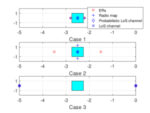
Figure 1: Optimized UAV positioning locations with $K=2$ ERs, in which the blue cube denotes an obstacle.

IV Numerical Results

This section provides numerical results to validate the performance of our proposed radio-map-based robust positioning design. In the simulation, we consider the segment propagation channel model [12], where if there are obstacles between the UAV and ER $k$, the channel follows a NLoS model with the path loss exponent being $\alpha_{\text{NLoS}}=4$ and reference channel power gain being $\beta_{\text{NLoS}}=10^{-4}$, and otherwise, the channel is LoS with the path loss exponent being $\alpha_{\text{LoS}}=2.3$ and reference channel power gain being $\beta_{\text{LoS}}=10^{-3}$. Unless otherwise stated, we set the UAV altitude as $H=\text{5 m}$, the maximum transmit power as $P=\text{10 W}$ and the prespecified ER location error as $\epsilon=\text{1 m}$. For performance comparison, we also consider the conventional LoS channel and probabilistic LoS channel, where we set the channel parameters as $\alpha_{0}=2$, $\beta_{0}=10^{-3}$, $A=10$, $B=0.6$ and $\eta=0.1$, which approximately match our obstacles’ distribution (please refer to [8] on the details of the channel parameters).

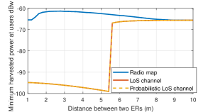
Figure 2: The common received power at each ER with $K=2$ ERs.

First, we consider the case with $K=2$ ERs as shown in Fig. 1, where there is one obstacle (i.e., the blue cube) between the two ERs with height 4.5 m. It is observed that when the two ERs’ distance is short (e.g., Cases 1 and 2), the optimized UAV positioning locations under the radio-map based design are different from those based on conventional LoS and probabilistic LoS models, in order to avoid the link blocking due to obstacles. By contrast, when the ERs’ distance becomes large (e.g., Case 3), the three approaches are observed to lead to similar positioning locations. Fig. 2 shows the average minimum or common received power versus the ERs’ distance. It is observed that when the distance is sufficiently large, the performances under the three schemes are almost same. When the distance becomes shorter, our proposed radio-map-based channel is observed to considerably outperform the conventional designs with LoS and probabilistic LoS channels. This is consistent with Fig. 1, in which our proposed design can efficiently find UAV positioning locations with LoS links to ERs, by exploiting the exact channel propagation information based on the radio map.

Next, we consider the setup with $K=5$ ERs located in an area of $10\times 10$ square meters as shown in Fig. 3, in which the blue cubes denote the obstacles (e.g., trees) with height 4.5 m. It is observed that under the radio-map-based design, there are three optimal positioning locations, which are close to ERs 1-2, ERs 3-4, and ER 5 with LoS connections, respectively. By contrast, under the LoS/probabilistic LoS channel models, the links between the UAV and ground ERs 1-4 are observed to be blocked by obstacles, resulting in severe performance loss. This is because either the deterministic LoS or the stochastic probabilistic LoS channel models cannot capture the specific features of the real channel environment, which comprises the performance. Fig. 4 shows the average minimum energy transferred to the $K$ ERs versus different transmit power $P$. It is observed that radio-map-based approach achieves approximately $100\%$ performance gain over the other two approaches in the case with $P=\text{10 W}$ and $40\%$ in the case with $P=\text{15 W}$.

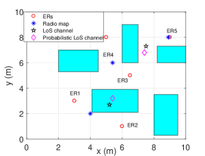
Figure 3: Optimized UAV positioning locations with $K=5$ ERs, in which blue cubes denote obstacles.

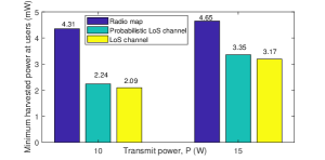
Figure 4: The max-min average received power at each ER versus the transmit power P with $K=5$ ERs.

V Conclusion

This letter studied a new radio-map-based robust positioning optimization approach for a UAV-enabled multiuser WPT system. We maximized the minimum energy transferred to all ERs over a sufficiently long charging period, by assuming that the UAV only partially knows the ER’s locations. We proposed to use the radio map technique to acquire the channel propagation information, and then adopted the robust optimization and Lagrange duality method to solve this problem efficiently. Numerical results showed that our proposed radio-map-based design achieved significant performance gains against other benchmark designs under LoS and probabilistic LoS channels. This is due to the fact that our proposed design can better exploit the channel propagation environment information, while the LoS/probabilistic LoS models generally mismatch with the real radio environment.

References

- [1] Y. Zeng, R. Zhang, and T. J. Lim, “Wireless communications with unmanned aerial vehicles: Opportunities and challenges,” IEEE Commun. Mag., vol. 54, no. 5, pp. 36–42, May 2016.
- [2] Y. Zeng, B. Clerckx, and R. Zhang, “Communications and signals design for wireless power transmission,” IEEE Trans. Commun., vol. 65, no. 5, pp. 2264–2290, May 2017.
- [3] J. Xu, Y. Zeng, and R. Zhang,“UAV-enabled wireless power transfer: Trajectory design and energy optimization,” IEEE Trans. Wireless Commun., vol. 17, no. 8, pp. 5092–5106, Aug. 2018.
- [4] L. Xie, J. Xu, and R. Zhang, “Throughput maximization for UAV-enabled wireless powered communication networks,” to appear in IEEE Internet Things J. , 2019.
- [5] S. Cho, K. Lee, B. Kang, K. Koo, and I. Joe, “Weighted harvest-then-transmit: UAV-enabled wireless powered communication networks,” IEEE Access, vol. 6, pp. 72212–72224, Nov. 2018.
- [6] M. Jiang, Y. Li, Q. Zhang, and J. Qin, “Joint position and time allocation optimization of UAV-enabled wireless powered communication networks,” to appear in IEEE Trans. Commun., 2019.
- [7] F. Zhou, Y. Wu, R. Q. Hu, and Y. Qian, “Computation rate maximization in UAV-enabled wireless-powered mobile-edge computing systems,” IEEE J. Sel. Areas Commun., vol. 36, no. 9, pp. 1927–1941, Aug. 2018.
- [8] A. Al-Hourani, S. Kandeepan, and S. Lardner, “Optimal LAP altitude for maximum coverage,” IEEE Wireless Commun. Lett., vol. 3, no. 6, pp. 569–572, Jul. 2014.
- [9] M. Mozaffari, W. Saad, M. Bennis, and M. Debbah, “Efficient deployment of multiple unmanned aerial vehicles for optimal wireless coverage,” IEEE Commun. Lett., vol. 20, no. 8, pp. 1647–1650, Aug. 2016.
- [10] O. Esrafilian, R. Gangula, and D. Gesbert, “Learning to communicate in UAV-aided wireless networks: Map-based approaches,” to appear in IEEE Internet Things J., 2019.
- [11] S. Bi, J. Lyu, Z. Ding, and R. Zhang, “Engineering radio maps for wireless resource management,” to appear in IEEE Wireless Commun., 2019.
- [12] J. Chen and D. Gesbert, “Optimal positioning of flying relays for wireless networks: A LOS map approach,” in Proc. IEEE ICC, Jul. 2017.
- [13] W. Yu and R. Lui, “Dual methods for nonconvex spectrum optimization of multicarrier systems,” IEEE Trans. Commun., vol. 54, no. 7, pp. 1310– 1322, Jul. 2006.
- [14] S. Boyd and L. Vandenberghe, Convex Optimization, Cambridge, U.K.:Cambridge Univ. Press, Mar. 2004.
- [15] S. Boyd. EE364b Convex Optimization II, Course Notes, accessed on Jun. 29 2017. [Online]. Available: http://www.stanford.edu/class/ee364b/