A far-UV survey of three hot, metal-polluted white dwarf stars: WD0455-282, WD0621-376, and WD2211-495

Abstract

Using newly obtained high-resolution data ($R\sim{1\times{10}^{5}}$) from the Hubble Space Telescope, and archival UV data from the Far Ultraviolet Spectroscopic Explorer we have conducted a detailed UV survey of the three hot, metal-polluted white dwarfs WD0455-282, WD0621-376, and WD2211-495. Using bespoke model atmospheres we measured $T_{\mathrm{eff}}$, log $g$, and photospheric abundances for these stars. In conjunction with data from Gaia we measured masses, radii, and gravitational redshift velocities for our sample of objects. We compared the measured photospheric abundances with those predicted by radiative levitation theory, and found that the observed Si abundances in all three white dwarfs, and the observed Fe abundances in WD0621-376 and WD2211-495, were larger than those predicted by an order of magnitude. These findings imply not only an external origin for the metals, but also ongoing accretion, as the metals not supported by radiative levitation would sink on extremely short timescales. We measured the radial velocities of several absorption features along the line of sight to the three objects in our sample, allowing us to determine the velocities of the photospheric and interstellar components along the line of sight for each star. Interestingly, we made detections of circumstellar absorption along the line of sight to WD0455-282 with three velocity components. To our knowledge, this is the first such detection of multi-component circumstellar absorption along the line of sight to a white dwarf.

1 Introduction

White dwarf stars are ubiquitous throughout the galaxy, and mark the final stage of evolution for main sequence stars with masses $<8-10M_{\odot}$ (Iben & Tutukov, 1997). As they no longer produce heat through nuclear fusion, white dwarfs spend the rest of their lives cooling to background temperature via the emission of radiation. Through the use of calculated evolution tables, the temperature of a white dwarf can be effectively used as a means to measure how long the star has been cooling. Approximately 30-50% of white dwarf stars are thought to have atmospheres polluted with metals (Barstow et al., 2014; Koester et al., 2014) (B14 and K14 hereafter). The mechanisms by which this pollution occurs is relatively well understood in the case of cool white dwarfs. The diffusion timescales for metals in these cases can be on the order of days for hydrogen-rich (DA) white dwarfs with effective temperatures ($T_{\mathrm{eff}}$) ranging between 12,000$<T_{\mathrm{eff}}<$20,000K (Paquette et al., 2002). Therefore, for metals to be observed in the atmosphere, the reservoir of material has to be continually replenished through accretion. However, in the case of hot white dwarfs ($T_{\mathrm{eff}}>$20,000K) the physics becomes more complex. In this case, the radiative forces in the atmosphere are efficient enough to overcome the gravitational stratification, resulting in metals such as C, N, O, and heavier being present in the photosphere through a process known as radiative levitation. In addition, as with the cool white dwarfs, accretion can also occur. Therefore, the observed photospheric abundance patterns in hot white dwarf stars will be a delicate balance between the flow of material sinking under gravity, the resistance to this flow from radiative levitation, and the introduction of additional material from accretion. Attempts have been made by Chayer et al. (2002b); Chayer et al. (2002a); Chayer et al. (2002c) (Ch94/95 hereafter) to use radiative levitation theory to predict the observed abundance patterns in white dwarf stars, however, it has often been the case that these predictions bear little resemblance to what is observed. This is a consequence of the assumptions made. In particular, Ch94/95 assumed that the reservoir of material available to be levitated was effectively infinite.

The evidence for accretion into the atmospheres of white dwarf stars is compelling. A study by K14 analysed the atmospheres of 85 white dwarf stars with $17,000<T_{\mathrm{eff}}<27,000$K. From this sample, 48 out of the 85 (56%) white dwarfs analysed were found to have signatures of metals in their atmospheres. Of these 48 metal-polluted white dwarfs, the photospheric compositions of 25 of these stars could be explained by radiative levitation alone. However, for the other 23 stars, K14 concluded that active accretion was taking place to account for the observed abundance patterns. B14 conducted a survey of 89 DA white dwarfs observed by the Far Ultraviolet Spectroscopic Explorer (FUSE) with $16,000<T_{\mathrm{eff}}<77,000$K. In this sample, 33 out of 89 white dwarfs were found to have atmospheres polluted with metals. In an attempt to understand the nature of this metal pollution, the authors compared the measured photospheric abundances to those predicted by Ch94/95. Out of the 33 white dwarfs considered, 12 were found to have enhanced Si abundances relative to the predicted radiative levitation abundances, implying an external origin. Further investigating this, B14 looked at the ratios of abundances for each star, such as Si/C, Si/P, and Si/S. The authors then compared these ratios to those seen in bulk-Earth material, in CI chondrites, and in the sun. It was shown that the white dwarf Si/C ratios were similar to those observed in CI chondrite material, further implying that metal pollution in hot white dwarf stars originates from rocky bodies.

In the case of cooler white dwarfs ($T_{\mathrm{eff}}<20,000$K) where radiative levitation is inefficient, comparing photospheric abundance ratios such as C/O to those observed in other types of media allows the origin of the material to be inferred. Wilson et al. (2016) measured the photospheric compositions of 16 white dwarf stars with $17,000<T_{\mathrm{eff}}<23,000$K and calculated the C/O ratio for each object. The authors found that four of these objects had C/O ratios coincident with that observed in bulk-Earth material, and five of these objects had C/O ratios coincident with that observed in chondrite material. Other authors have also used this technique to study the compositions of accreted material such as Kawka & Vennes (2016); Zuckerman et al. (2011); Xu et al. (2014). As well as photospheric abundance measurements for cool white dwarfs, observational data has revealed the presence of dusty debris disks orbiting white dwarf stars. An excellent example of this is the metal polluted white dwarf SDSS 1228+1040. Using time-resolved spectroscopic data from the William Herschel Telescope Gänsicke et al. (2006) detected emission features from the Ca ii triplet with laboratory wavelengths 8498, 8542, and 8662Å. The authors also found this emission did not vary over timescales of 20 minutes to one day. The authors concluded that this emission arose from a gaseous circumstellar disk around the white dwarf. More exotic cases of debris disks have been observed, such as that of WD1145+017. Using high cadence photometry, Vanderburg et al. (2015) made the surprising discovery that not only did WD1145+017 have a debris disk, this disk was found to be composed of several disintegrating objects. As this debris transits the white dwarf, it causes the star’s brightness to dim by up to 40%. Further studies such as those by Rappaport et al. (2016); Gänsicke et al. (2016); Xu et al. (2016); Croll et al. (2015) have focused on characterising the type and compositions of the objects orbiting WD1145+017. Most recently, new observations by Manser (2019) of SDSS 1228+1040 have revealed the presence of an Fe-core planetesimal orbiting the white dwarf.

The extensive literature concerning the accretion of metals onto cool white dwarf stars is compelling. However, the question of the origin of metal pollution in hot white dwarfs is still an open question. In this paper we present our photospheric and interstellar survey of three hot, DA white dwarfs stars, namely WD0455-282, WD0621-376, and WD2211-495. First, we describe new Hubble Space Telescope observations obtained for the three white dwarfs, as well as archival Far Ultraviolet Spectroscopic Explorer (FUSE) data. We then describe the model atmosphere calculations performed, and how these were used to measure the effective temperature, surface gravity, and photospheric compositions of the stars. We then conduct a line survey of the three objects, and identify the velocity populations present along the line of sight to the white dwarfs. We then discuss the results obtained, and consider the photospheric compositions of the white dwarfs in the context of radiative levitation. We also discuss the results of the interstellar survey. Lastly, we make concluding remarks, and detail the future work planned.

2 Observations

WD0455-282, WD0621-376, and WD2211-495 were observed using the Space Telescope Imaging Spectrometer (STIS) aboard the Hubble Space Telescope as part of program GO-14791. Each star was observed using the E140H FUV/MAMA echelle grating (nominal resolution $R={\lambda}/{\Delta\lambda}\sim 1{\times}10^{5}$, Martin & Baltimore 2012), with a 0.2x0.2 aperture. The aperture size was chosen so as to maximise the flux throughput. Further, special, deeper than normal, exposures of the wavelength calibration lamp were taken to aid in the assignment of precise wavelength scales. The STIS echellegram reduction and co-addition procedures we adopted have been fully described in a previous paper (Hu et al., 2018). In brief, the raw spectral datasets were processed through a version of the STIS pipeline with a number of specially updated reference files, including new dispersion solutions for the specific grating settings used. The individual echelle orders of the processed echellegrams were then concatenated, imposing an active blaze correction to ensure optimum flux continuity across the overlapping zones of the adjacent orders. If multiple sub-exposures were taken in a given grating setting, these were co-added after aligning relative to the leading spectrum by cross-correlation. Finally, the overlapping regions between the two separate grating settings (1307Å  and 1416Å) were adjusted to match the fluxes and again aligned in wavelength by cross-correlation. The alignment shifts typically were small, often only 0.1 km s^-1 in magnitude. The final wavelength coverage for the spliced spectra was approximately 1200$-$1520Å. The average signal-to-noise ratio per resolution element ($\sim$3 km s^-1) in the co-added spectra ranged from about 35 (WD0455-282) to 60–70 (WD2211-495 and WD0621-376, respectively). We summarise the STIS observations for each star in Table 1, and plot the STIS spectra of each object in Figure 1.

Figure 1: STIS spectra obtained for WD0455-282, WD0621-376, and WD2211-495. The spectra have been normalised by the flux at 1300Å, and offset from each other for clarity.

Table 1: List of spectral datasets obtained from the HST for each object using STIS with the E140H grating. $\lambda_{c}$ is the central wavelength of the exposure. The start time is given in the Universal Time Zone (UT).

Object	Observation ID	Start Time/Date	$\lambda_{c}$ (Å)	Exposure time (s)
WD0455-282	OD7QD0IUQ	05:43:21 15/08/2017	1307	2487.0
	OD7QD0JDQ	07:15:40 15/08/2017	1307	2964.0
	OD7QD0JHQ	08:51:06 15/08/2017	1307	2964.0
	OD7QD1010	10:29:50 15/08/2017	1416	2487.0
	OD7QD1020	12:02:00 15/08/2017	1416	2964.0
	OD7QD1030	13:37:26 15/08/2017	1416	2964.0
WD0621-376	OD7QC0H5Q	02:40:08 10/10/2017	1307	2525.0
	OD7QC0HRQ	04:04:42 10/10/2017	1307	3002.0
	OD7QC0030	05:42:08 10/10/2017	1416	2881.0
	OD7QC0030	07:15:33 10/10/2017	1416	3002.0
WD2211-495	OD7QA0MRQ	05:49:44 15/10/2017	1307	2610.0
	OD7QA0020	07:19:07 15/10/2017	1416	2966.0

To complement our STIS observations, and provide a means with which to measure the effective temperature ($T_{\mathrm{eff}}$) and surface gravity (log $g$) for the three objects, we constructed high signal-to-noise spectra using archival observations from the Far Ultraviolet Spectroscopic Explorer (FUSE). We summarise the FUSE exposures used in this work in Table 2, and plot the FUSE spectra for each object in Figure 2. Unlike STIS, which uses echelle-blaze optics, FUSE used four individual mirrors to reflect light onto two detectors, resulting in eight individual spectra (see Moos et al. 2002). Collectively, these exposures spanned 905-1184Å, and encompassed the H-Lyman series from Ly-$\beta$, down to the lyman limit ($\sim{911}$Å). There were three apertures available to use. These were the LWRS (low resolution, 30’x30’), MDRS (medium resolution, 4’x20’), and HIRS (high-resolution, 1.25’x20’) apertures with resolutions ranging from 15,000 to 21,000. After FUSE launched, it became evident that there were distortions present in the optical design, caused by heating and cooling of the individual components. This resulted in the eight spectra having different wavelength shifts. In addition, these distortions meant that the object being observed often drifted out of the field of view when the MDRS and HIRS apertures were used. This resulted in the flux of the observed spectra being attenuated by arbitrary amounts. Therefore, when constructing the spectra for this work, we only included observations where the LWRS aperture was used where possible. In the case of WD0455-282 where MDRS observations were used, we omitted exposures where the flux was attenuated, or where there was no flux at all.

We note that, in addition to the FUSE and HST datasets, there also exists UV spectroscopy from the International Ultraviolet Explorer (IUE), with a resolution $\sim{1\times{10}^{4}}$. IUE data for the three objects considered in this paper were analysed by Holberg et al. (2002), who catalogued the various absorption features observed in their respective spectra. We opt not to use these IUE data in favour of the higher resolution FUSE and STIS data described hitherto.

Figure 2: FUSE spectra obtained for WD0455-282, WD0621-376, and WD2211-495. The spectra have been normalised by the flux at 1052Å, and offset from each other for clarity.

Table 2: List of spectral datasets obtained from FUSE for each object. The start time is given in theUniversal Time Zone (UT).

Object	Observation ID	Exposures	Start Time/Date	Aperture	Exposure time (s)
WD0455-282	P10411010	15	02:14:28 03/02/2000	MDRS	19667.0
	P10411020	8	05:07:49 04/02/2000	MDRS	10122.0
	P10411020	13	09:36:51 07/02/2000	MDRS	17675.0
WD0621-376	P10415010	19	05:28:58 06/12/2000	LWRS	8371.0
WD2211-495	M10303020	5	17:18:58 21/10/1999	LWRS	2720.0
	M10303030	9	19:43:40 25/10/1999	LWRS	4160.0
	M10303040	7	21:45:44 01/11/1999	LWRS	2976.0
	M10303050	11	06:55:16 03/06/2000	LWRS	5157.0
	M10303060	8	05:15:34 29/06/2000	LWRS	4193.0
	M10303070	12	20:43:02 17/08/2000	LWRS	5260.0
	M10303080	9	06:09:32 24/10/2000	LWRS	3954.0
	M10303090	11	09:29:25 24/10/2000	LWRS	5025.0
	M10303100	9	12:49:19 24/10/2000	LWRS	5795.0
	M10303110	13	05:28:46 25/10/2000	LWRS	5877.0
	M10303120	11	10:28:36 25/10/2000	LWRS	5430.0
	M10303130	8	04:07:07 01/08/2002	LWRS	3796.0
	M10303140	7	14:23:40 10/06/2002	LWRS	3774.0
	M10303150	10	17:20:00 25/09/2002	LWRS	5460.0
	M10303160	13	23:28:41 24/05/2002	LWRS	6929.0
	M10303180	12	04:14:39 17/09/2003	LWRS	5875.0
	M10315010	7	18:26:46 07/05/2004	LWRS	3699.0
	M10315040	7	17:27:33 06/07/2004	LWRS	3889.0

3 Stellar atmosphere models

All model atmospheres described in this paper were calculated using the non-LTE model atmosphere code tlusty, version 201 (Hubeny, 1988; Hubeny & Lanz, 2002). Synthetic spectra were then generated from these model atmospheres using synspec Hubeny & Lanz (2011). These spectra spanned 900-1600Å, and were convolved with an instrumental Gaussian profile whose FWHM (full-width, half maximum) was dependent upon the observational data being considered. For FUSE data, the FWHM was set to 0.0641Å, and for the STIS data the FWHM was calculated as $\lambda/114,000$ as given in the STIS instrument manual. The H-Lyman absorption profiles were calculated using the Stark Broadening tables of Tremblay & Bergeron (2009). These tables are an updated version of the tables presented in Lemke (2003), including non-ideal effects such as those resulting from perturbations to the absorber due to protons and electrons.

Given the high temperature of the white dwarf stars considered, we have created new model ions for C, N, O, Si, P, and S to account for the presence of higher ionization states. For the model atmospheres calculated, we include model ions for C i-v, N i-vi, O i-vii, Si i-viii, P i-viii, S i-viii, Fe iii-vii, and Ni iii-vii. In addition, we also include single-level ions for C vi, N vii, O viii, Si ix, P ix, S ix, Fe viii, and Ni viii.

Full line-blanketing effects for $>9,000,000$ transitions of Fe and Ni are accounted for via the opacity sampling method. For Fe, the atomic data including energy levels and transitions originates from Kurucz (1992), and the photoionization cross sections (PICS) from the Opacity Project (Seaton et al., 2014). For Ni, the atomic data also originates from Kurucz (1992), and the PICS for Ni vii were calculated using an hydrogenic approximation. For Ni iv-vi we use the PICs calculated by Preval et al. (2017).

4 Methodology

4.1 General photospheric parameter measurement

It is currently untenable to calculate model atmosphere grids that can account for variations in $T_{\mathrm{eff}}$, log $g$, and all of the individual abundances simultaneously. To do so would require the calculation of thousands, if not millions, of stellar atmospheric models that incorporate the various possible permutations of these variables. Therefore, for each star, we adopted an iterative procedure to determine the best fitting values of these parameters. First, we calculated a starting NLTE model atmosphere with tlusty using values of $T_{\mathrm{eff}}$, log $g$, and metal abundances from Barstow et al. (2003) and B14. Then, for each metal abundance we wanted to measure, we used synspec to calculate a grid of model atmospheres with different abundances by stepping away from the starting model in LTE. We then measured the abundances using these grids. Once we measured the abundances, we used tlusty to calculate an NLTE model atmosphere grid with these abundances, varying in $T_{\mathrm{eff}}$ and log $g$. We then measured $T_{\mathrm{eff}}$ and log $g$ using the H-Lyman lines. After measuring $T_{\mathrm{eff}}$ and log $g$, we calculated an NLTE model atmosphere using the measured $T_{\mathrm{eff}}$, log $g$, and metal abundances. We then repeated the aforementioned steps until the measured $T_{\mathrm{eff}}$, log $g$, and metal abundances were converged. Our convergence criterion was defined such that the difference between the parameters measured in the previous and current iterations were less than their measurement uncertainties. In total, we performed seven iterations for WD0455-282, and six iterations for WD0621-376 and WD2211-495. Below, we describe how the metal abundances, $T_{\mathrm{eff}}$, and log $g$ were measured in more detail.

4.2 $T_{\mathrm{eff}}$, log $g$, and abundance measurements

In Table 3 we list the transitions used to measure the abundances of C, N, O, Si, P, S, Fe, and Ni. Fe and Ni are difficult metals for which to measure an abundance. This is because the atomic data can be quite uncertain with respect to their centroid wavelengths, broadening parameters, and oscillator strengths. In an attempt to mitigate this, we used 8–10 Fe v and Ni v transitions, and simultaneously fit all of these lines to find the best abundance value. We note that for our abundance determinations we use only one ionization state per ion. Generally, wherever possible, we have tried to use lines arising from transitions between excited states. This is because resonant transitions have been known to be accompanied by high ionization state ISM lines (also termed “circumstellar”, see Bannister et al. 2003; Dickinson et al. 2012) which can potentially compromise the abundance measurement. We discuss the lines used, and the reason why they were used here. In the case of C, only the C iii transitions were visible in the spectra considered. For N, the N iv multiplet is present at 912-915Å, however, these lines are in a region of spectrum where the signal-to-noise is sub optimal. In addition, the multiplet is contaminated by interstellar H. Therefore, we opt to use only the N v doublet. For O there are three O iv lines and one O v line ($\sim{1371}$Å) that can be used. In this case, we opted to use the O iv lines simply because there were more lines to use. For Si the Si iii ionization state has a low population relative to Si iv due to the temperatures of the objects considered ($>60,000$K). For P, the P v ionization state is the most populated relative to P iv, again due to the temperatures of the objects considered. For S, the S vi resonant transitions are detected at 933Å  and 945Å. However, these lines are in close proximity to Ly-$\delta$ and Ly-$\epsilon$, meaning they are sensitive to the wings of these H lines. In addition, abundance measurements made using these S vi lines have been shown to be in great disagreement with measurements made using S iv and Sv (see, for example, Preval et al. 2013). Lastly, for Fe and Ni, the strongest lines come from Fe v and Ni v. Only a few Fe/Ni vi lines are visible in the spectrum that could potentially be used. Therefore, we opted to use the Fe/Ni v lines due to the number of these lines available.

The STIS spectra used in this work have $>$50,000 data points. Reading in, and fitting all of these data points is very computationally demanding. Therefore, we opted to fit individual transitions by extracting a section of spectrum encompassing the feature we want to measure. The wavelength regions extracted for each transition were the same for all three stars, and are listed in Table 3. To measure the individual metal abundances, we used the X-Ray spectral analysis package xspec (Arnaud, 1996), which uses a $\chi^{2}$ minimisation procedure to interpolate a model grid to the observed data, and determine the best fitting values for these parameters with the reduced $\chi^{2}$ value ($\chi^{2}_{\mathrm{red}}$) being as close to unity as possible. To ensure we obtained the best fitting abundance values, we calculated $\chi^{2}_{\mathrm{red}}$ over all abundance values in the model grid.

Table 3: List of transitions used to measure the photospheric abundances of the three white dwarfs considered. Transitions with wavelengths in the STIS range (1200-1520Å) were used to measure the photospheric velocity.

Ion	Wavelength (Å)	log $gf$	Extracted Region (Å)
C iii	1174.933	-0.468	1170–1180
C iii	1175.263	-0.565	1170–1180
C iii	1175.590	-0.690	1170–1180
C iii	1175.711	0.009	1170–1180
C iii	1175.987	-0.565	1170–1180
C iii	1176.370	-0.468	1170–1180
C iii	1247.383	-0.314	1245–1255
N v	1238.821	-0.505	1235–1245
N v	1242.804	-0.807	1235–1245
O iv	1338.615	-0.632	1335–1350
O iv	1342.990	-1.333	1335–1350
O iv	1343.514	-0.380	1335–1350
Si iv	1122.485	0.220	1115–1130
Si iv	1128.340	0.470	1115–1130
Si iv	1393.755	0.030	1390–1405
Si iv	1402.770	-0.280	1390–1405
P v	1117.977	-0.010	1115–1130
P v	1128.008	-0.320	1115–1130
S v	1501.760	-0.489	1495–1505
Fe v	1320.409	0.243	1315–1325
Fe v	1387.937	0.660	1385–1395
Fe v	1402.385	0.229	1390–1405
Fe v	1430.572	0.597	1425–1435
Fe v	1440.528	0.448	1440–1450
Fe v	1446.617	0.468	1440–1450
Fe v	1448.847	0.309	1440–1450
Fe v	1455.555	0.277	1450–1460
Fe v	1456.162	0.173	1450–1460
Fe v	1464.686	0.471	1460–1470
Ni v	1257.626	0.585	1255–1265
Ni v	1261.760	0.478	1255–1265
Ni v	1273.204	0.395	1265–1275
Ni v	1279.720	0.300	1275–1290
Ni v	1300.979	-0.048	1295–1305
Ni v	1307.603	0.168	1305–1315
Ni v	1318.515	0.307	1315–1325
Ni v	1336.136	0.557	1335–1345
Ni v	1342.176	0.345	1335–1345

To measure the $T_{\mathrm{eff}}$ and log $g$ of each star, we first extracted wavelength regions from FUSE spectra encompassing four Lyman lines, namely Ly-$\beta$, Ly-$\gamma$, Ly-$\delta$, and Ly-$\epsilon$. Ly-$\alpha$ is present in the STIS data, however, this line cannot be used to measure $T_{\mathrm{eff}}$ and log $g$ due to contamination from interstellar H absorption. In the extracted spectra, we removed erroneous photospheric and interstellar absorption features. We then used XSPEC to interpolate our $T_{\mathrm{eff}}$/log $g$ model grids to the Lyman lines.

The statistical uncertainties on the abundances, $T_{\mathrm{eff}}$, and log $g$ were determined by considering the change in $\chi^{2}$. For the abundances, the uncertainties were obtained by reading off the abundance values for which $\Delta\chi^{2}=1$ corresponding to a $1\sigma$ confidence interval for one variable parameter. It should be noted that the abundance uncertainties do not account for the uncertainty in the $T_{\mathrm{eff}}$ and log $g$ measurement. This is because in the iteration scheme, $T_{\mathrm{eff}}$ and log $g$ are held fixed for abundance measurements. For $T_{\mathrm{eff}}$ and log $g$, the uncertainties were calculated by reading off the $T_{\mathrm{eff}}$ and log $g$ values for which $\Delta\chi^{2}=2.2957$ corresponding to a $1\sigma$ confidence interval for two variable parameters. The statistical uncertainties on quantities measured in this work are dependent upon the uncertainty on the observed flux. In the case of FUSE data, the uncertainty on the observed flux can be greatly underestimated due to calibration issues with the instruments (Moos et al., 2002). Therefore, to determine the uncertainties on quantities measured using FUSE data, a few, additional steps were required. First, we fit the observed data by interpolating the model grids with xspec. This results in a $\chi_{\mathrm{red}}^{2}$ value not equal to unity. Then, we expressed the flux uncertainties as a fractional percentage of the observed flux (e.g. 2.5%). We then varied this fractional percentage so as to obtain a $\chi_{\mathrm{red}}^{2}$ of unity. We then determined the uncertainty on the relevant quantities by reading off the $T_{\mathrm{eff}}$/log $g$ values corresponding to $\Delta\chi^{2}=2.2957$, and the abundance values corresponding to $\Delta\chi^{2}=1.0$.

4.3 Astrophysical & astrometric quantities

With the second data release from the astrometric observatory Gaia, the positions and parallaxes of hundreds of thousands of white dwarfs are now known to milli- and micro-arcsecond precision. Using parallax data information from Gaia, the observed STIS spectrum, and our best fitting synthetic spectrum, we can measure the radius $R_{*}$ of the white dwarf. The distance $D$ in parsecs to the white dwarf is calculated as $\overline{\omega}$:

$$D=\frac{1000}{\overline{\omega}}.$$ (1)

where $\overline{\omega}$ is the parallax in milliarcseconds. Then, $R_{*}$ is calculated as

$$R_{*}=D\sqrt{\frac{F_{\lambda}}{4\pi{H}_{\lambda}}}$$ (2)

where $F_{\lambda}$ is the observed flux, and $H_{\lambda}$ is the Eddington flux as obtained from the synthetic spectrum of the white dwarf in question. $F_{\lambda}$ and $H_{\lambda}$ are functions of wavelength. Therefore, we adopted a statistical approach to find the best value for $F_{\lambda}/H_{\lambda}$. Firstly, we extracted a region of spectrum from the synthetic and observed datasets where there were relatively few absorption features. We found that the region 1480-1500Å  is suitable. We then calculated the mean value of $F_{\lambda}/H_{\lambda}$, weighted by their reciprocal squared errors. This value was then used to determine $R_{*}$. With $R_{*}$ and log $g$, we can then determine the mass of the white dwarf, $M_{WD}$, calculated as

$$M_{\mathrm{WD}}=\frac{gR_{*}^{2}}{G}$$ (3)

where $G$ is the universal gravitational constant. Finally, with the mass and radius, we can then find the gravitational redshift $z_{\mathrm{gr}}$. In velocity units, the redshift, $V_{\mathrm{gr}}$, is calculated as

$$V_{\mathrm{gr}}=cz_{\mathrm{gr}}=\frac{GM_{*}}{cR_{*}}$$ (4)

where $c$ is the speed of light.

4.4 Velocity measurements

The exceptional calibration and resolution of STIS allows for the precise measurement of the photospheric (or radial) and interstellar velocities of the three white dwarfs. When measuring the abundances of the various metal absorption features, xspec shifts the synthetic spectrum in wavelength space to find the best fit to the data. To measure the photospheric velocity, we calculate the average velocity of all the transitions in the STIS data listed in Table 3. The uncertainty in the velocity measurement is then determined by calculating the standard deviation of the velocities.

Again, thanks to the high-resolution of the STIS spectra, it is possible to separate blended ISM features into their individual components. While a detailed study of these features quantifying column densities and temperatures is beyond the scope of this work, we do, however, measure the velocities of these features. To measure the velocities of the ISM lines we fit Gaussian profiles to the observed absorption features, parameterised by the wavelength centroid, the absorption depth, and the Doppler width. The exact parameterisation is given in the Appendix. The advantage to the profile used is that it can account for line saturation. The best fitting parameters were determined by using a $\chi^{2}$ minimization procedure as implemented in the idl package mpfit (Markwardt, 2009). The interstellar velocity was measured by calculating the average of the measured velocities of the lines listed in Table 4, weighted by their inverse square errors. The uncertainty on the weighted ISM component was determined by calculating the standard deviation of the measured velocities. When we found evidence of multiple component ISM absorption, we calculated the average velocities of lines with similar velocities. We note that there are ISM lines that exist in the FUSE spectra of our objects. However, we opted not to use these lines in our velocity measurements due to the lower-accuracy wavelength calibration in the FUSE spectra.

Table 4: List of transitions used to measure the ISM velocities along the line of sight to the white dwarfs.

Ion	Wavelength (Å)	log $gf$
N i	1200.22329	-0.4589
N i	1200.70981	-0.7625
Si iii	1206.4995	0.2057
Si ii	1260.4221	0.3911
O i	1302.16848	-0.6195
Si ii	1304.3702	-0.7329
C ii	1334.5323	-0.5912

5 Results - Photospheric Survey

In this section we present the results of our photospheric survey. Using the lines listed in Table 3, we measured a photospheric velocity of $81.5\pm 1.9$, $37.4\pm 1.8$, and $30.0\pm 1.7$ km s^-1 for WD0455-282, WD0621-376, and WD2211-495 respectively. In Table 5 we summarise the measured stellar parameters for each star, including $T_{\mathrm{eff}}$, log $g$, $M_{*}$,$R_{*}$, and the photospheric abundances. The abundances are expressed as number fractions of hydrogen. All uncertainties quoted are to one sigma. In this section we first discuss the abundance measurements made for each species detected in the three white dwarfs. We then present measurements for $T_{\mathrm{eff}}$/log $g$ for each star. In conjunction with data from the astrometric satellite Gaia, we then give direct measurements of the distances, masses, radii, and gravitational redshifts for each object.

Table 5: List of measured parameters for WD0455-282, WD0621-376, and WD2211-495. RA, Dec, $G$, $G_{\mathrm{BP}}$, $G_{\mathrm{RP}}$, and Parallax data taken from Gaia DR2. Note that the RA/Dec coordinates are in the ICRS reference, and the epoch is J2015.5. Bolometric magnitudes, and cooling ages were determined using the Montreal Cooling tables (see Holberg & Bergeron 2006).

Parameter	WD0455-282	WD0621-376	WD2211-495
$T_{\mathrm{eff}}$ (K)	$65400_{-1210}^{+1240}$	$64500_{-424}^{+437}$	$65900_{-254}^{+259}$
Log $g$ (cgs)	$7.87_{-0.09}^{+0.09}$	$7.60_{-0.03}^{+0.03}$	$7.58_{-0.02}^{+0.02}$
$v_{\mathrm{phot}}$ (km s-1)	$81.5\pm 1.9$	$37.4\pm 1.8$	$30.0\pm 1.7$
RA (deg)	$74.30575\pm 0.25388$	$95.80294\pm 0.04720$	$333.54973\pm 0.04232$
Dec (deg)	$-28.13127\pm 0.31315$	$-37.69113\pm 0.05733$	$-49.32451\pm 0.06189$
Gaia $G$	$13.915\pm 0.002$	$12.041\pm 0.002$	$11.610\pm 0.002$
Gaia $G_{\mathrm{BP}}$	$13.651\pm 0.009$	$11.789\pm 0.013$	$11.315\pm 0.007$
Gaia $G_{\mathrm{RP}}$	$14.236\pm 0.003$	$12.382\pm 0.003$	$11.951\pm 0.002$
Johnson $V$	$13.901\pm 0.023^{{\dagger}}$	$12.063\pm 0.020^{{\dagger}}$	$11.667\pm 0.031^{{\dagger}}$
$M_{\mathrm{Bol}}$	$3.220\pm 0.190$	$2.778\pm 0.064$	$2.641\pm 0.042$
Cooling Age (Myr)	$0.96\pm 0.07$	$0.82\pm 0.03$	$0.76\pm 0.02$
Parallax (mas)	$8.237\pm 0.354$	$13.136\pm 0.059$	$16.992\pm 0.082$
Distance (pc)	$121\pm 5$	$76.1\pm 0.3$	$58.9\pm 0.3$
Mass ($M_{\odot}$)	$0.589\pm 0.145$	$0.731\pm 0.053$	$0.575\pm 0.028$
Radius (${R}_{\odot}/100$)	$1.48\pm 0.06$	$2.24\pm 0.01$	$2.04\pm 0.01$
$V_{\mathrm{grav}}$ (km s-1)	$25.4\pm 6.3$	$20.7\pm 1.5$	$18.0\pm 0.9$
N(C)/N(H)	$1.00\times{10}^{-8}$	$1.49_{-0.08}^{+0.08}\times{10}^{-6}$	$5.05_{-0.55}^{+0.55}\times{10}^{-7}$
N(N)/N(H)	$7.71_{-0.21}^{+0.21}\times{10}^{-8}$	$6.45_{-0.12}^{+0.12}\times{10}^{-7}$	$1.49_{-0.05}^{+0.05}\times{10}^{-6}$
N(O)/N(H)	$1.58_{-0.12}^{+0.12}\times{10}^{-7}$	$2.46_{-0.03}^{+0.03}\times{10}^{-6}$	$2.00_{-0.03}^{+0.03}\times{10}^{-6}$
N(Si)/N(H)	$9.18_{-0.29}^{+0.29}\times{10}^{-7}$	$8.75_{-0.19}^{+0.18}\times{10}^{-6}$	$4.38_{-0.15}^{+0.15}\times{10}^{-6}$
N(P)/N(H)	$7.58_{-0.46}^{+0.46}\times{10}^{-8}$	$1.70_{-0.16}^{+0.16}\times{10}^{-7}$	$1.73_{-0.07}^{+0.07}\times{10}^{-7}$
N(S)/N(H)	$2.70_{-0.25}^{+0.25}\times{10}^{-7}$	$1.05_{-0.06}^{+0.15}\times{10}^{-6}$	$8.06_{-0.47}^{+0.46}\times{10}^{-7}$
N(Fe)/N(H)	$2.72_{-0.11}^{+0.11}\times{10}^{-6}$	$1.84_{-0.04}^{+0.04}\times{10}^{-5}$	$1.21_{-0.04}^{+0.04}\times{10}^{-5}$
N(Ni)/N(H)	$7.96_{-0.27}^{+0.27}\times{10}^{-7}$	$4.78_{-0.08}^{+0.08}\times{10}^{-6}$	$3.32_{-0.10}^{+0.10}\times{10}^{-6}$
†The AAVSO Photometric All Sky Survey (APASS) DR9, Henden et al. (2016).

5.1 C Abundance

In Figure 3 we have plotted the FUSE spectra of the three white dwarfs spanning 1174-1178Å  which contains the C iii multiplet transition. Interestingly, we find no traces of this multiplet in the spectrum of WD0455-282. Therefore, we place a limit on the photospheric C abundance in this star of $<1.00\times{10}^{-8}$. The C iii multiplet is only just visible in the cases of WD0621-376 and WD2211-495. As mentioned previously, the uncertainties for the FUSE data are unreliable. Therefore, when measuring the C abundance, we expressed the flux uncertainty as a fraction of the observed flux so as to achieve a fit with $\chi_{\mathrm{red}}^{2}$ close to unity. We measure photospheric C abundances of $1.49_{-0.08}^{+0.08}\times{10}^{-6}$ and $5.05_{-0.55}^{+0.55}\times{10}^{-7}$ for WD0621-376 and WD2211-495 respectively.

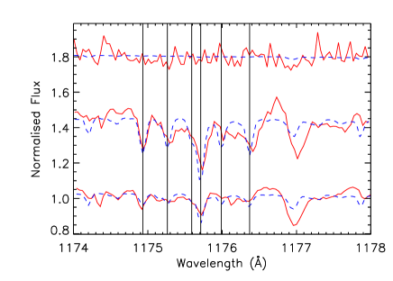
Figure 3: Section of FUSE spectra for WD0455-282 (top), WD0621-376 (middle), and WD2211-495 (bottom) containing the C iii multiplet shifted to rest wavelength. The flux for each white dwarf has been normalised, and offset for clarity. The red solid line is the observed flux, while the blue dashed line is the best fitting photospheric model. The vertical solid lines indicate the positions of the transitions used to measure the abundance.

5.2 N Abundance

In Figure 4 we have plotted a region of the STIS spectra for the three white dwarfs containing the N v doublet. We detected the N iv multiplet in the FUSE spectra at 914-918Å  for all three stars, however, the signal-to-noise in this region was too low to measure an accurate abundance. The N v doublet is clearly resolved in all three stars, and we measure N abundances of $7.71_{-0.21}^{+0.21}\times{10}^{-8}$, $6.45_{-0.12}^{+0.12}\times{10}^{-7}$, and $1.49_{-0.05}^{+0.05}\times{10}^{-6}$ for WD0455-282, WD0621-376, and WD2211-495 respectively.

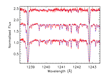
Figure 4: Section of the STIS spectrum from WD0455-282 (top), WD0621-376 (middle) and WD2211-495 (bottom) containing the N v doublet. The fluxes have been normalised, and offset from each other for clarity. Note that the observed flux has been shifted to rest wavelength. The red-solid line is the observational data, while the blue dashed line is the best fitting photospheric model. The vertical black lines indicate the position of the N v doublet used to measure the abundances.

5.3 O Abundance

In Figure 5 we have plotted the region of STIS spectrum containing two of the O iv transitions used to measure the O abundance for WD0455-282, WD0621-376, and WD2211-495. The O v line at 1371Å  was also detected, however, we opted to use the O iv lines as there were three lines to fit. We measured O abundances of $1.58_{-0.12}^{+0.12}\times{10}^{-7}$, $2.46_{-0.03}^{+0.03}\times{10}^{-6}$, and $2.00_{-0.03}^{+0.03}\times{10}^{-6}$ for WD0455-282, WD0621-376, and WD2211-495 respectively. In Figure 6 we have plotted a region of STIS spectrum containing the O v 1371.296Å  line for the three white dwarfs. Excellent agreement is seen between the synthetic and observed spectrum for WD0621-376. However, for WD0455-282 and WD2211-495 it can be seen that the synthetic profile for O v doesn’t descend all the way into the observed profile. This implies the $T_{\mathrm{eff}}$ may be underestimated for these stars. This may be due to our convergence criteria being too relaxed, where iterations of $T_{\mathrm{eff}}$, log $g$, and abundance measurements were performed until the difference between the previous and current measurements was less than the uncertainty on the measurement.

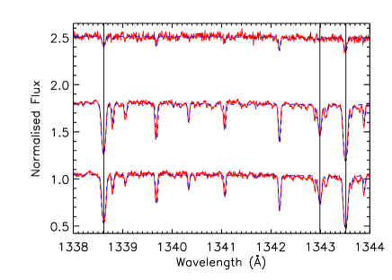
Figure 5: The same as for Figure 4, but for a region of the STIS spectrum containing three O iv lines with laboratory wavelengths 1338.615, 1342.990, and 1343.514Å  respectively.

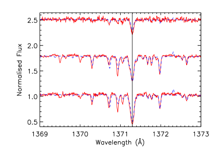
Figure 6: The same as for Figure 4, but for a region of the STIS spectrum containing an O v line with laboratory wavelength 1371.296Å.

5.4 Si Abundance

In Figure 7 we have plotted the region of STIS spectrum containing the resonant Si iv doublet for WD0455-282, WD0621-376, and WD2211-495. In addition to the STIS data, we also used two excited Si iv absorption features from the FUSE spectrum. As was the case with the C iii transition, we expressed the FUSE flux uncertainty as a fraction of the observed flux so as to achieve a fit with $\chi_{\mathrm{red}}^{2}$ close to unity. We measured Si abundances of $9.18_{-0.29}^{+0.29}\times{10}^{-7}$, $8.75_{-0.19}^{+0.18}\times{10}^{-6}$, and $4.38_{-0.15}^{+0.15}\times{10}^{-6}$ for WD0455-282, WD0621-376, and WD2211-495 respectively. We note that our Si abundance measurements for WD0621-376 and WD2211-495 are an order of magnitude larger than that of B14, who measured $7.57_{-0.31}^{+0.31}\times{10}^{-7}$ and $2.41_{-2.04}^{+5.21}\times{10}^{-7}$ respectively. For WD0621-376 we defer discussion until later in the paper. However, in the case of WD2211-495 this large difference may be due to the higher quality observational data used in this work. For comparison, B14 used a FUSE spectrum constructed with one dataset (M10303160), whereas the present work uses a FUSE spectrum with 18 datasets (see Table 2).

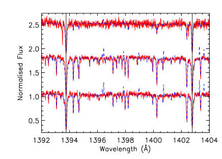
Figure 7: The same as for Figure 4, but for a region of the STIS spectrum containing two Si iv lines with laboratory wavelengths 1393.755 and 1402.770Å. For WD0455-282, the additional absorption feature next to the photospheric profile is a circumstellar line, whose discussion is deferred to Section 10.

5.5 P Abundance

In Figure 8 we have plotted the region of FUSE spectra for the three white dwarfs that contains the P v resonant doublet. As was the case for the C iii multiplet, we expressed the flux uncertainties in the FUSE data as a fraction of the observed flux so as to achieve a fit with $\chi_{\mathrm{red}}^{2}$ close to unity. We measured the photospheric P abundance to be $7.58_{-0.46}^{+0.46}\times{10}^{-8}$, $1.70_{-0.16}^{+0.16}\times{10}^{-7}$, and $1.73_{-0.07}^{+0.07}\times{10}^{-7}$ for WD0455-282, WD0621-376, and WD2211-495 respectively.

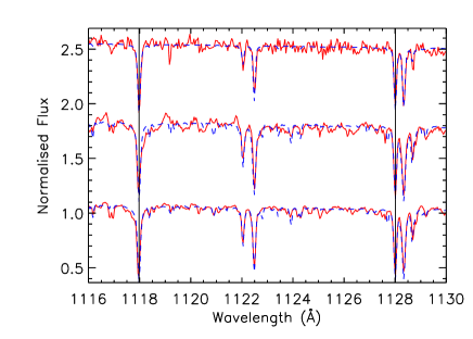
Figure 8: The same as for Figure 3, but for a region of the FUSE spectrum containing two P v lines with laboratory wavelengths 1117.977 and 1128.008Å  respectively.

5.6 S Abundance

In Figure 9 we have plotted the region of STIS spectrum containing the excited S v transition for the three white dwarfs. The resonant S vi doublet is detected in the FUSE spectra, however, we opted not to use these for abundance measurements. This is because they are situated close to the line centroids of the Lyman series where the wings are changing rapidly, meaning the abundance will be sensitive to the broadening of the Lyman lines. We measured an S abundance of $2.70_{-0.25}^{+0.25}\times{10}^{-7}$, $1.05_{-0.06}^{+0.15}\times{10}^{-6}$, and $8.06_{-0.47}^{+0.46}\times{10}^{-7}$ for WD0455-282, WD0621-376, and WD2211-495 respectively.

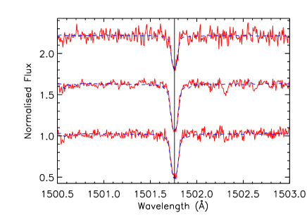
Figure 9: The same as for Figure 4, but for a region of the STIS spectrum containing the S v line with laboratory wavelength 1501.760Å.

5.7 Fe Abundance

In Figure 10 we have plotted a region of the STIS spectrum containing two of the Fe v lines used to measure the Fe abundance in the three white dwarfs. We measured Fe abundances of $2.72_{-0.11}^{+0.11}\times{10}^{-6}$, $1.84_{-0.04}^{+0.04}\times{10}^{-5}$, and $1.21_{-0.04}^{+0.04}\times{10}^{-5}$ for WD0455-282, WD0621-376, and WD2211-495 respectively. In Figure 11 we have also plotted a region of STIS spectrum containing three Fe vi absorption features with laboratory wavelengths 1295.817, 1296.734 and 1296.872Å  respectively for the three white dwarfs. As with the case of O v, excellent agreement is seen between the observed and synthetic spectra for WD0621-376, while the synthetic spectra for WD0455-282 and WD2211-495 do not descend completely into the observed spectrum.

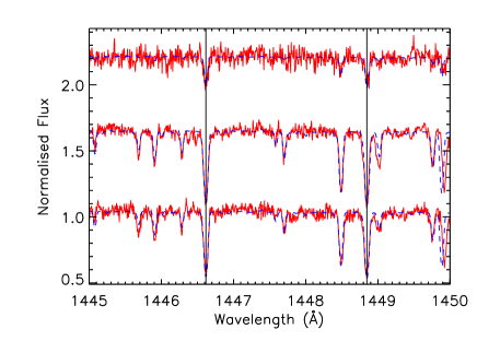
Figure 10: The same as for Figure 4, but for a region of STIS spectrum containing two Fe v lines with laboratory wavelengths 1446.617 and 1448.847Å  respectively.

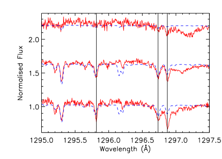
Figure 11: The same as for Figure 4, but for a region of STIS spectrum containing three Fe vi lines with laboratory wavelengths 1295.817, 1296.734 and 1296.872Å  respectively.

5.8 Ni Abundance

In Figure 12 we have plotted a region of the STIS spectrum containing one of the Ni v features used to measure the Ni abundance in the three white dwarfs. We measured Ni abundances of $7.96_{-0.27}^{+0.27}\times{10}^{-7}$, $4.78_{-0.08}^{+0.08}\times{10}^{-6}$, and $3.32_{-0.10}^{+0.10}\times{10}^{-6}$ for WD0455-282, WD0621-376, and WD2211-495 respectively.

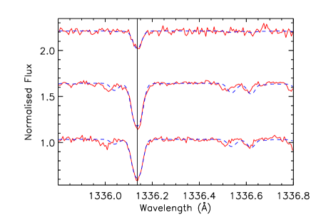
Figure 12: The same as for Figure 4, but for a region of STIS spectrum containing an Ni v line with laboratory wavelength 1336.136Å.

5.9 $T_{\mathrm{eff}}$/log $g$ measurements

The Lyman lines (Ly-$\beta$ - Ly-$\epsilon$) used to measure $T_{\mathrm{eff}}$ and log $g$ are located in the FUSE spectrum. As mentioned previously, the flux uncertainties in the FUSE spectra are unreliable. Therefore, we express the flux uncertainties as a fraction of the observational flux so as to achieve a fit with $\chi_{\mathrm{red}}^{2}$ close to unity. For $T_{\mathrm{eff}}$, we measured values of $65400_{-1210}^{+1240}$, $64500_{-424}^{+437}$, and $65900_{-254}^{+259}$K for WD0455-282, WD0621-376, and WD2211-495 respectively. For log $g$, we measured values of $7.87_{-0.09}^{+0.09}$, $7.60_{-0.03}^{+0.03}$, and $7.58_{-0.02}^{+0.02}$ for WD0455-282, WD0621-376, and WD2211-495 respectively. Interestingly, we noted that the log $g$ measurement for WD0621-376 is much higher than reported in previous works. Indeed, B14 measured log $g=7.22$ for this star.

5.10 Mass-radius measurements

Prior to the launch of the astrometric satellite Gaia, measurement of astrophysical parameters such as the mass and radius of a white dwarf required the use of theoretical cooling tables such as those calculated by Holberg & Bergeron (2006); Kowalski & Saumon (2006); Tremblay et al. (2011); Bergeron et al. (2011) (Montreal cooling tables hereafter). Thanks to the highly accurate parallax measurements made by Gaia, the angular diameter of any field white dwarf can be measured to a high degree of precision. Combined with the distance, we can then extract the radius, and in conjunction with log $g$, we can then obtain the mass, followed by the gravitational redshift velocity. These mass and radius measurements offer a valuable means with which to test the fundamental mass-radius relationship for white dwarf stars.

For WD0455-282, the Gaia DR2 parallax was measured to be $8.237\pm 0.354$mas, corresponding to a distance of $121\pm 5$pc. Using equations 2 and 3, we extracted a mass and radius of $0.589\pm 0.145M_{\odot}$ and $1.48\pm 0.06R_{\odot}/100$ respectively. The large uncertainty on the mass is dominated by the uncertainty on our log $g$ measurement. With the mass and radius, we then calculated a gravitational redshift velocity of $25.4\pm 6.3$ km s^-1.

For WD0621-376, the Gaia DR2 parallax is $13.136\pm 0.059$mas, corresponding to a distance of $76.1\pm 0.3$pc. With these values, we measured a mass and radius of $0.731\pm 0.053M_{\odot}$ and $2.24\pm 0.01R_{\odot}/100$ respectively. Using the mass and radius, we measured the gravitational redshift velocity to be $20.7\pm 1.5$ km s^-1. We are skeptical of our mass measurement due to the large difference between our measured log $g$ (7.60), and that of Barstow et al. (2014) (7.22). If we use log $g$=7.22 in Equation 3 then the measured mass decreases to $0.305M_{\odot}$. We defer further exploration of this issue to the discussion.

For WD2211-495 the measured Gaia DR2 parallax is $16.992\pm 0.082$mas, corresponding to a distance of $58.9\pm 0.3$pc, making the star the closest in our sample. With this information, we measured the mass and radius to be $0.575\pm 0.028M_{\odot}$ and $2.04\pm 0.01R_{\odot}/100$ respectively. Using the mass and radius, we then calculated the gravitational redshift velocity to be $18.0\pm 0.9$ km s^-1.

6 Results - Interstellar Survey

In this section we present the results of our interstellar survey. To aid classification of the detected features, we used the Dynamical Local ISM calculator, the theory and motivation for which is described by Redfield & Linsky (2008). The calculator is freely available online, and gives an indication of what interstellar clouds may be traversed along the line of sight given a galactic latitude, and longitude. The calculator also predicts the velocity components of the cloud in question. In Table 6 we summarise the detected velocity components, and the clouds intersected by the line of sight.

Table 6: List of measured ISM velocities for WD0455-282, WD0621-376, and WD2211-495, and the (known) clouds intersected by the line of sight.

Parameter	WD0455-282	WD0621-376	WD2211-495
No of components	4	2	2
$V_{i}$ (km s-1)	$-40.3\pm 1.6$, $-32.1\pm 3.0$	$12.1\pm 2.3$, $23.1\pm 2.4$	$-9.91\pm 1.39$, $-2.18\pm 2.43$
	$16.7\pm 1.9$, $25.1\pm 1.1$
Clouds intersected	Blue	Blue	LIC

6.1 WD0455-282

The line of sight to WD0455-282 appears to have a very interesting structure. In our line survey we detected four distinct ISM velocity components, with average velocities of $v_{1}=-40.3\pm 1.6$, $v_{2}=-32.1\pm 3.0$, $v_{3}=16.7\pm 1.9$, and $v_{4}=25.1\pm 1.1$ km s^-1 respectively. In Figure 13 we have plotted a region of STIS spectrum for WD0455-282 containing the Si ii 1260Å  transition, where all four velocity components can be seen. We measured the four velocities to be $-40.7\pm 0.2$, $-35.7\pm 2.2$, $17.9\pm 1.2$, and $25.7\pm 1.3$ km s^-1 respectively. The LISM calculator states that the light of sight towards WD0455-282 traverses the Blue cloud, which has a radial velocity of $12.6\pm 1.0$ km s^-1. While this velocity is close to our measurement for $v_{3}$, the two values are not in agreement.

Interestingly, our survey of WD0455-282 has revealed the presence of multi-component circumstellar absorption in the Si iii 1206, Si iv 1393, and 1402Å  resonant lines. In Figs 14, 15, and 16 we have plotted three spectral regions containing the Si iii and Si iv resonant lines, along with our best fit to these data using Gaussian profiles. The Si iii 1206Å  line has three circumstellar components with velocities of $-32.8\pm 0.4$, $12.8\pm 1.3$, and $23.4\pm 0.3$ km s^-1 respectively. Si iv 1393Å  has two circumstellar components with velocities of $17.3\pm 4.9$ and $25.9\pm 0.2$ respectively. Lastly, the Si iv 1402Å  line has two circumstellar components with velocities of $16.1\pm 1.4$ and $25.3\pm 0.4$ respectively. For the Si iii line, the circumstellar velocities are strikingly similar to those measured for the ISM velocities $v_{2}$, $v_{3}$, and $v_{4}$. For Si iv the circumstellar velocities are similar to those measured for $v_{3}$ and $v_{4}$. To our knowledge, this is the first time that multi-component circumstellar absorption has been observed along the line of sight to a white dwarf star.

Figure 13: Best fit to the absorption features detected between 1260.2 to 1260.7Å  using 6 Gauss profiles for WD0455-282. From left to right, the first two features correspond to interstellar Si ii with velocities of $-40.7\pm 0.2$ and $-35.7\pm 2.2$ km s^-1 respectively. The third feature is a photospheric line, and the last two features are interstellar Si ii with velocities of $17.9\pm 1.2$ and $25.7\pm 1.3$ km s^-1 respectively.

Figure 14: Best fit to the absorption features detected between 1206.2 and 1206.7Å  using 3 Gauss profiles for WD0455-282. All three features arise from Si iii 1206Å, with velocities of $-32.8\pm 0.4$, $12.8\pm 1.3$, and $23.4\pm 0.3$ km s^-1. All three components are circumstellar.

Figure 15: Best fit to the absorption features detected between 1393.7 and 1394.3Å  using 3 Gauss profiles for WD0455-282. All three features arise from Si iv 1393Å, with velocities $17.3\pm 4.9$, $25.9\pm 0.2$, and $80.9\pm 0.2$ km s^-1. The first two components are interstellar, and the third component is photospheric.

Figure 16: Best fit to the absorption features detected between 1402.5 and 1403.4Å  using 3 Gauss profiles for WD0455-282. The latter three features arise from Si iv 1402Å, with velocities of $16.1\pm 1.4$, $25.3\pm 0.4$, and $80.6\pm 0.2$ km s^-1 respectively. The absorption feature on the far left is a photospheric Fe line. The second and third components are circumstellar Si iv, and the fourth component is photospheric Si iv.

6.2 WD0621-376

We made detections of two distinct ISM velocity components along the line of sight to WD0621-376 with average velocities of $v_{1}=12.1\pm 2.3$, and $v_{2}=23.1\pm 2.4$ km s^-1 respectively. The LISM calculator indicated the line of sight to WD0621-376 intersects the Blue cloud, with a predicted radial velocity of $11.1\pm 0.9$ km s^-1. Based on this value, our first ISM component appears to originate from the Blue cloud. In Figure 17 we have plotted a region of spectrum containing the Si ii 1260Å  transition, where both ISM components can be seen with velocities of $14.0\pm 0.3$ and $23.2\pm 0.3$ km s^-1 respectively.

Unlike WD0455-282, we didn’t detect any circumstellar features along the line of sight to WD0621-376. In addition, we made no detections of the Si iii 1206.4995Å  transition. The significance of this result will be explored shortly.

Figure 17: Best fit to the absorption features detected between 1260.2 to 1260.7Å  using three Gauss profiles for WD0621-376. The first two features are interstellar Si ii with velocities of $14.0\pm 0.3$ and $23.2\pm 0.3$ km s^-1 respectively, while the third feature is a photospheric line.

6.3 WD2211-495

We have identified two distinct ISM velocity components along the line of sight to WD2211-495, with average velocities of $v_{1}=-9.91\pm 1.39$ and $v_{2}=-2.18\pm 2.43$ km s^-1 respectively. In Figure 18 we have plotted a region of STIS spectrum for WD2211-495 containing the C ii 1334Å  line, where both ISM components can be seen with velocities of $-11.7\pm 0.8$ and $1.67\pm 0.85$ km s^-1 respectively. The LISM calculator indicated that the line of sight traversed two clouds, namely the Local Interstellar Cloud (LIC), and the Dor cloud, with velocities $-8.80\pm 1.32$ and $9.93\pm 0.60$ km s^-1 respectively. Our first ISM velocity is in agreement with the value predicted for the LIC, suggesting this component is associated with the LIC. However, our last component is not in agreement with the Dor cloud velocity. This maybe due to a limitation in the LISM model, which is based upon four sightlines for the Dor Cloud (contrast with 79 sightlines for the LIC, and 10 for the Blue cloud). This could also be explained if the Dor cloud does not intersect the line of sight to the white dwarf.

We made a detection of a single circumstellar component in the Si iii 1206 line, and the Si iv 1393Å  line. We do not detect a circumstellar line in the Si iv 1402Å  line due to the presence of strong Fe/Ni absorption features. In Figs 19 and 20 we have plotted regions of STIS spectra for WD2211-495 encompassing the Si iii and Si iv transitions respectively. We measured the velocity of the circumstellar component to be $3.43\pm 0.10$ km s^-1 for the Si iii line, and $-1.00\pm 0.56$ km s^-1 for the Si iv line. The measured circumstellar velocities are similar to the velocity measured for the ISM component $v_{2}$.

Figure 18: Best fit to the absorption features detected between 1334.2 to 1334.7Å  using three Gauss profiles for WD2211-495. The first feature is photospheric, while the second and third features are interstellar C ii with velocities of $-11.7\pm 0.8$, and $1.67\pm 0.85$ km s^-1 respectively.

Figure 19: Best fit to the absorption features detected between 1206 and 1207Å  using 1 Gauss profile for WD2211-495. This feature is circumstellar Si iii, with a velocity of $3.43\pm 0.10$ km s^-1.

Figure 20: Best fit to the absorption features detected between 1393.7 and 1394.3Å  using 2 Gauss profiles for WD2211-495. The first feature is circumstellar Si iv with a velocity of $-1.00\pm 0.56$ km s^-1, while the second feature is photospheric Si iv with a velocity of $29.3\pm 0.12$ km s^-1.

7 Discussion: Radiative levitation

It is well established that metals are able to be supported against gravitational diffusion in white dwarf atmospheres thanks to radiative levitation. The efficiency of radiative levitation is a sensitive function of $T_{\mathrm{eff}}$ and log $g$, meaning the observed abundance patterns in a white dwarf atmosphere will also be a function of $T_{\mathrm{eff}}$ and log $g$ (neglecting accretion). In Figure 21 we have plotted the measured abundances in all three white dwarfs as number fractions of H. A general trend can be seen for all three objects, where the abundance of the metals increases steadily from C to Si, followed by a drop for the P abundance, followed by a steady increase again for S to Fe. It can also be seen that the abundance curves for WD0621-376 and WD2211-495 overlap one another. Furthermore, because WD0455-282 has a similar abundance pattern to the other two white dwarfs, it appears that the WD0455-282 curve can be brought up to meet the other two curves through the application of a multiplicative constant. This is simply explained by considering the $T_{\mathrm{eff}}$ and log $g$ values for each white dwarf. The measured $T_{\mathrm{eff}}$ and log $g$ for WD0621-376 and WD2211-495 are very similar. Therefore, material in the atmospheres of these two stars will experience a similar radiative acceleration. WD0455-282 has a similar $T_{\mathrm{eff}}$, but a higher log $g$, meaning the equilibrium abundances will be smaller in this object compared to the other two. This point is further reinforced by considering the Fe/Ni abundance ratio. The Fe/Ni ratios observed in WD0455-282, WD0621-376, and WD2211-495 were calculated to be $3.42_{-0.18}^{+0.18}$, $3.85_{-0.10}^{+0.10}$, and $3.64_{-0.16}^{+0.16}$ respectively. Within error the Fe/Ni ratio observed for WD2211-495 is in agreement with that observed for WD0621-376, while the ratio observed for WD0621-376 is in agreement with that observed for WD0455-282.

Figure 21: Plot of observed photospheric abundances for WD0455-282 (solid line, plus-symbols), WD0621-376 (dotted line, asterisk-symbols), and WD2211-495 (dashed line, diamond-symbols). Note that the C abundance for WD0455-282is an upper limit.

There is continuing disagreement between the photospheric abundances observed in white dwarf atmospheres, and the photospheric abundances predicted by radiative levitation theory. The most well-known set of radiative equilibrium abundances for white dwarf stars were calculated by Ch94/95. This disagreement is thought to be due to a number of simplifying assumptions used in calculating the abundances. These assumptions include assuming no momentum redistribution of levitated material, and that the reservoir of material that could be levitated was effectively infinite. However, these values are useful to compare against, as they define the maximum possible abundance that can be supported in the atmosphere through radiative levitation. In Table 7 we have tabulated the predicted abundances from radiative equilibrium theory, and compare them to the measured photospheric abundances from WD0455-282, WD0621-376, and WD2211-495. In all three stars, it can be seen that for C, N, O, P, S, and Ni the measured abundances are smaller than those predicted by Ch94/95. However, in the case of Si, the observed abundance is larger by several dex than those predicted by Ch94/95. As mentioned above, the abundances from radiative equilibrium theory will be the maximum possible abundance that can be supported through radiative levitation alone. Therefore, material exceeding this quantity should sink into the core. This implies that the reservoir of Si and Fe is being continually replenished.

In addition to the calculations performed by Ch94/95, more detailed models were considered by Landenberger-Schuh (2005) that included the effects of gravitational diffusion and radiative levitation in a self consistent manner. Schuh was able to show that the radiative support for Si plummets for DA white dwarfs with $T_{\mathrm{eff}}>60,000$K. This is because the population of Si iv decreases as Si v becomes populated with increasing temperature. This means there should be little to no Si present in the white dwarfs considered in this work. This corroborates the prediction by Ch94/95, providing further support to the idea that the three objects are potentially accreting material. However, it is not clear where this material originates from. The interplay between the flow of material sinking into the core via gravitational diffusion, the retardation of this flow by radiative levitation, and the introduction of additional material through accretion makes the problem complex. Therefore, this means that the methods used in studying metal pollution in cool white dwarfs (where radiative levitation is inefficient) cannot be applied to the stars studied in this paper. Future work will focus on developing the necessary computational and theoretical framework to study these processes, and how they affect the observed photospheric abundance patterns in white dwarf star atmospheres.

Table 7: Comparison between predicted photospheric abundances from radiative levitation theory (Ch94/95), and those measured in this work (Observed column) for WD0455-282, WD0621-376, and WD2211-495, as a number fraction relative to H.

	WD0455-282		WD0621-376		WD2211-495
N(X)/N(H)	Ch94/95	Observed	Ch94/95	Observed	Ch94/95	Observed
N(C)/N(H)	$1.51\times{10}^{-6}$	$1.00\times{10}^{-8}$	$2.82\times{10}^{-6}$	$1.49\times{10}^{-6}$	$3.02\times{10}^{-6}$	$5.05\times{10}^{-7}$
N(N)/N(H)	$3.72\times{10}^{-6}$	$7.71\times{10}^{-8}$	$6.76\times{10}^{-6}$	$6.45\times{10}^{-7}$	$7.76\times{10}^{-6}$	$1.49\times{10}^{-6}$
N(O)/N(H)	$4.07\times{10}^{-6}$	$1.58\times{10}^{-7}$	$7.24\times{10}^{-6}$	$2.46\times{10}^{-6}$	$8.32\times{10}^{-6}$	$2.00\times{10}^{-6}$
N(Si)/N(H)	$5.75\times{10}^{-9}$	$9.18\times{10}^{-7}$	$2.14\times{10}^{-8}$	$8.75\times{10}^{-6}$	$1.91\times{10}^{-8}$	$4.38\times{10}^{-6}$
N(P)/N(H)	$1.78\times{10}^{-6}$	$7.58\times{10}^{-8}$	$3.72\times{10}^{-6}$	$1.70\times{10}^{-7}$	$4.07\times{10}^{-6}$	$1.73\times{10}^{-7}$
N(S)/N(H)	$2.57\times{10}^{-6}$	$2.70\times{10}^{-7}$	$5.13\times{10}^{-6}$	$1.05\times{10}^{-6}$	$5.62\times{10}^{-6}$	$8.06\times{10}^{-7}$
N(Fe)/N(H)	$4.37\times{10}^{-6}$	$2.72\times{10}^{-6}$	$1.02\times{10}^{-5}$	$1.84\times{10}^{-5}$	$1.15\times{10}^{-5}$	$1.21\times{10}^{-5}$
N(Ni)/N(H)	$1.07\times{10}^{-4}$	$7.96\times{10}^{-7}$	$2.09\times{10}^{-4}$	$4.78\times{10}^{-6}$	$2.51\times{10}^{-4}$	$3.32\times{10}^{-6}$

8 Discussion: The mass-radius relationship

As mentioned previously the high-precision astrometric data from Gaia provides an excellent means with which to test the mass-radius relationship for white dwarf stars. In Figure 22 we have plotted our measured $T_{\mathrm{eff}}$/log $g$ values for the three white dwarfs, and the predicted $T_{\mathrm{eff}}$/log $g$ values from the Montreal cooling tables for white dwarfs with masses ranging from 0.5-0.7$M_{\odot}$. The cooling tables assume a thick H-envelope of $M_{\mathrm{H}}/M_{*}=1\times{10}^{-4}$, where $M_{\mathrm{H}}$ is the mass of the H-layer, and $M_{*}$ is the mass of the star. Using the best fitting synthetic spectrum and data from Gaia we measured the masses of WD0455-282, WD0621-376, and WD2211-495 to be $0.589\pm 0.145$, $0.731\pm 0.053$, and $0.575\pm 0.028M_{\odot}$ respectively. Comparatively, if we use the cooling tables to obtain the masses, we measure the masses to be $0.676\pm 0.033$, $0.576\pm 0.011$, and $0.572\pm 0.007M_{\odot}$ for WD0455-282, WD0621-376, and WD2211-495 respectively. For WD0455-282 and WD2211-495 the masses measured using Gaia data are in agreement within error with those measured using the cooling tables. However, there is a significant discrepancy in the case of WD0621-376. There are multiple potential explanations for this mass discrepancy, which we now consider in turn.

The first possibility concerns the accuracy of the parallax used in the measurement. Stassun & Torres (2018) found evidence of a $-82\pm 33\mu$as systematic offset in the Gaia DR2 parallaxes. As the calculated mass is dependent upon the radius, and, therefore, the parallax measurement, this shift will make the mass more uncertain. To check this, we applied this offset to the Gaia DR2 parallax for WD0621-376 and recalculated the mass. This results in a mass of $0.740\pm 0.053M_{\odot}$, showing that the parallax measurement is not the cause of the discrepancy. Further reinforcing this is the fact that WD0621-376 is not variable to within 0.0029mag (Marinoni et al., 2016), ruling out uncertainties on the parallax due to variability. A second possibility concerns interstellar reddening, which can affect the UV flux and introduce uncertainties in the measured $T_{\mathrm{eff}}$ and log $g$. However, using the 3D dust maps of Lallement et al. (2014), we find the extinction along the line of sight to WD0621-376 is negligible, and is unlikely to affect $T_{\mathrm{eff}}$ and log $g$. A third possibility is the thickness of the H envelope assumed in the model calculation. Using detailed pre-white dwarf evolutionary sequences Romero et al. (2019) showed that the thickness of this envelope decreases as the total mass of the star increases, leading to a decrease in the radius of the star of up to $\sim{12}$%. However, this effect is too small to explain the discrepant mass. Lastly, a fourth possibility is that the STIS spectrum is poorly calibrated. As an additional check, the V magnitude can be used to determine the mass of WD0621-376. This has the advantage of using optical rather than UV fluxes. In this case, the ratio $F_{\lambda}/H_{\lambda}$ seen in Equation 2 is calculated by determining the flux $F_{\lambda}$ in the V-band:

$$F_{\lambda}=F_{0}\times{10}^{-0.4V},$$ (5)

where $V$ is the V-magnitude, $\lambda=5423$Å, $F_{0}=3.804\times{10}^{-9}$ (see table 15 in Holberg & Bergeron 2006), and $H_{\lambda}$ is the Eddington flux at $\lambda=5423$Å. The mass is then calculated using Equation 3. By using $V=12.063\pm 0.020$ from Table 5 we calculate the mass to be $0.804\pm 0.018M_{\odot}$. This is slightly larger than the value measured using the STIS data. This shows that the STIS calibration is not the cause of the discrepant mass value.

The origin of this mass discrepancy is currently unknown, and requires further study. This mass discrepancy could originate from the so-called Lyman/Balmer line problem described in Barstow et al. (2003), where the measured $T_{\mathrm{eff}}$/log $g$ values for a DA white dwarf differ depending on whether the Lyman or Balmer lines are used. We plan to explore this further in future work.

Figure 22: Comparison of the measured values of $T_{\mathrm{eff}}$/log $g$ for the three white dwarfs with the montreal cooling curves for white dwarfs with masses ranging from 0.5-0.7M_⊙. For comparison, the masses measured for WD0455-282, WD0621-376, and WD2211-495 were $0.589\pm 0.145$, $0.731\pm 0.053$, and $0.575\pm 0.028M_{\odot}$ respectively.

9 Discussion: Discrepancies in WD0621-376

The large difference between our value of log $g$ and that measured by B14 for WD0621-376 is a mystery. As well as the disagreement between our log $g$ measurement and that of B14, there is also disagreement with the value measured by Gianninas et al. (2010). Using the Balmer H-lines, the authors measured log $g=7.12$. The disagreement between the optical and UV log $g$ measurements is not surprising as this has been seen in other stars as a consequence of the Lyman/Balmer line problem. A detailed discussion of the problem is beyond the scope of this paper. Despite the large disagreement between the various log $g$ measurements, we are confident that our measured $T_{\mathrm{eff}}$ for WD0621-376 is correct. This is because the ionization equilibria for O iv and O v are in excellent agreement with the observational data in Figures 5 and 6 respectively. This can also be seen in the case of Fe v and Fe vi in Figures 10 and 11 respectively.

Our measured log $g$ should at least be similar to that measured by B14 as we both used the same FUSE dataset (P10415010). However, the FUSE spectrum used in this work was constructed independently of B14. To see if using different spectra resulted in the discrepancy we measured $T_{\mathrm{eff}}$ and log $g$ of WD0621-376 using the same reduced FUSE spectrum as B14. For this measurement we used the $T_{\mathrm{eff}}$/log $g$ grid from the final iteration in this work for WD0621-376. Using the B14 spectrum we measured $T_{\mathrm{eff}}=64800_{-521}^{+504}$K, and log $g=7.63_{-0.03}^{+0.03}$. Compared with the values measured in this work of $T_{\mathrm{eff}}=64500_{-424}^{+437}$K and log $g=7.60_{-0.03}^{+0.03}$, the two results are in good agreement implying the log $g$ discrepancy does not originate from the dataset used.

The large uncertainty in log $g$ for WD0621-376 will also introduce large uncertainties in the measured abundances. To gauge this effect we re-measured the metal abundances for WD0621-376 using a model atmosphere with log $g=7.22$. The method used is the same as described in Section 4.1. We set $T_{\mathrm{eff}}=63900$K as measured from the Lyman lines. In Table 8 we list the measured abundances for WD0621-376 when using a model atmosphere with log $g=7.60$, and when using a model atmosphere with log $g=7.22$. We also list the % difference between the two abundance measurements, calculated as

$$\%\,\mathrm{Difference}=100\frac{(X-X_{0})}{X_{0}},$$ (6)

where $X$ is the abundance measured using the log $g=7.22$ model, and $X_{0}$ is the abundance measured using the log $g=7.60$ model. It can be seen that the C, N, O, Fe, and Ni abundances are highly sensitive to the different log $g$ values, with the abundance difference between the two models being 50.1, -53.7, -30.7, -46.5, and -42.7% respectively. The Si, P, and S abundances are much less sensitive, with the abundance differences being 5.86, -0.19, and -17.1% respectively.

The insensitivity of the Si abundance to log $g$ is surprising. In Section 5.4 we noted that our Si abundance measurement for WD0621-376 was an order of magnitude larger than that measured by B14. Given the large difference between the log $g$ values measured in this work and in B14, we would have expected at least some dependence upon log $g$. Based on this fact, and the other factors hitherto discussed, it appears that the discrepancies described in this paper arises as a result of the stellar atmosphere grid used to make the measurements. Several differences exist between the model grids used in B14 and those used in the present work. Firstly, the models calculated in this work included more model atoms/ions than the B14 work, and covered a wider range of ionization states. Secondly, the Ni ions in this work used the photoionization cross sections calculated by Preval et al. (2017) using autostructure (Badnell, 2011), whereas the B14 models used hydrogenic photoionization cross sections. Thirdly, the model grids used in the B14 study were not calculated based on an iterative scheme. In this case, the model grids calculated by B14 varied in $T_{\mathrm{eff}}$, log $g$, and metal abundance scaled by a multiplicative factor. Future work will be focused on a detailed exploration of all of these differences.

Table 8: Comparison of metal abundances measured for WD0621-376 using a model atmosphere with log $g=7.60$, and log $g=7.22$. Both models have $T_{\mathrm{eff}}=64500$K. We have tabulated the % difference between the measured abundances, defined in text.

N(X)/N(H)	log $g=7.60$	log $g=7.22$	% Difference
N(C)/N(H)	$1.49_{-0.08}^{+0.08}\times{10}^{-6}$	$2.24_{-0.09}^{+0.09}\times{10}^{-6}$	50.1
N(N)/N(H)	$6.45_{-0.12}^{+0.12}\times{10}^{-7}$	$2.99_{-0.03}^{+0.04}\times{10}^{-7}$	-53.7
N(O)/N(H)	$2.46_{-0.03}^{+0.03}\times{10}^{-6}$	$1.70_{-0.03}^{+0.03}\times{10}^{-6}$	-30.7
N(Si)/N(H)	$8.75_{-0.19}^{+0.18}\times{10}^{-6}$	$9.27_{-0.17}^{+0.17}\times{10}^{-6}$	5.86
N(P)/N(H)	$1.70_{-0.16}^{+0.16}\times{10}^{-7}$	$1.69_{-0.16}^{+0.16}\times{10}^{-7}$	-0.19
N(S)/N(H)	$1.05_{-0.06}^{+0.15}\times{10}^{-6}$	$8.69_{-0.40}^{+0.39}\times{10}^{-7}$	-17.1
N(Fe)/N(H)	$1.84_{-0.04}^{+0.04}\times{10}^{-5}$	$9.85_{-0.10}^{+0.10}\times{10}^{-6}$	-46.5
N(Ni)/N(H)	$4.78_{-0.08}^{+0.08}\times{10}^{-6}$	$2.74_{-0.02}^{+0.02}\times{10}^{-6}$	-42.7

10 Discussion: Interstellar & Circumstellar absorption

The work presented in this paper has been valuable in terms of our understanding of circumstellar absorption. In Section 6 we discussed our detections of circumstellar absorption features in WD0455-282, WD0621-376 and WD2211-495. As seen in previous works on circumstellar features, the absorption features detected in this work are all blue-shifted with respect to the photospheric velocity. We made several interesting observations in our study of the circumstellar absorption features, which we now discuss in turn.

10.1 Si iii detections

Interestingly, while WD0455-282 and WD2211-495 showed signatures of circumstellar absorption, we made no detections of circumstellar absorption in the case of WD0621-376. However, the most interesting feature of this non-detection concerns the case of the Si iii resonant feature with laboratory wavelength 1206.4995Å. In the case of WD0621-376, we do not detect this feature at all, whereas for WD0455-282 and WD2211-495, we do detect this feature. Because of the high temperatures and gravities of the stars studied, absorption from the Si iii resonant transition in the photosphere will be very weak. This means that the feature shouldn’t be detected in any of the stars studied. Indeed, in a study by Preval et al. (2013), the authors also detected the Si iii resonant transition in high-resolution STIS spectra of the hot white dwarf G191-B2B (see figure. 9 in the paper). The authors also detected a circumstellar component in the C iv resonant doublet at 1548 and 1550Å, and in the Si iv resonant doublet at 1393 and 1402Å  (see figs. 5, 6, 10, and 11 in Preval et al. 2013). In the aforementioned works, Si iii has not previously been considered as a circumstellar line. However, in the context of the stellar atmospheric ionization fractions, this line can only be circumstellar. Therefore, this implies that the resonant Si iii line in hot white dwarfs could be a useful tracer of circumstellar absorption.

10.2 Relation to the interstellar medium

Previous studies such as those conducted by Bannister et al. (2003), Dickinson et al. (2012), and Preval et al. (2013) have attempted to understand the origin of circumstellar absorption using velocity discrimination. For example, as mentioned previously in the case of G191-B2B, the C iv doublet has both a photospheric and circumstellar component. Preval et al. (2013) measured the velocity the circumstellar components to be $8.26\pm 0.18$ km s^-1 for the 1548Å  line, and $8.30\pm 0.15$ km s^-1 for the 1550Å  line. The authors also measured the average velocity of two ISM components along the line of sight to G191-B2B using low ionization-state resonant transitions commonly found in the ISM. They measured the velocities of these two components to be $19.4\pm 0.03$ and $8.64\pm 0.03$ km s^-1 respectively. Redfield & Linsky (2008) showed that these two velocity components arise as a result of absorption from the LIC, and the Hyades cloud respectively. Interestingly, the velocity of the C iv circumstellar components are very similar to the velocity measured for the Hyades cloud, tentatively implying a connection between the two.

In the present work, four ISM velocity components were detected along the line of sight to WD0455-282 with velocities of $v_{1}=-40.3\pm 1.58$, $v_{2}=-32.1\pm 3.04$, $v_{3}=16.7\pm 1.85$, and $v_{4}=25.1\pm 1.06$ km s^-1 respectively. For the Si iii 1206Å  line, we detected three circumstellar components with velocities of $-32.8\pm 0.35$, $12.8\pm 1.25$, and $23.4\pm 0.25$ km s^-1 respectively. For the Si iv 1393Å  line, we detected two circumstellar components with velocities of $17.3\pm 4.89$ and $25.9\pm 0.23$ km s^-1 respectively. Finally, for the Si iv 1402Å  line, we detected two circumstellar components with velocities of $16.1\pm 1.43$ and $25.3\pm 0.36$ km s^-1 respectively. The similarity of the circumstellar velocities to the $v_{2}$, $v_{3}$, and $v_{4}$ components is difficult to miss, and, like G191-B2B, implies some connection.

In the case of WD2211-495 we detected two ISM components with velocities of $v_{1}=-9.91\pm 1.39$ and $v_{2}=-2.18\pm 2.43$ km s^-1 respectively. The velocity of the circumstellar component detected in the Si iii 1206Å  line was measured to be $3.43\pm 0.10$ km s^-1, and the velocity for the circumstellar component detected in the Si iv 1393Å  line was measured to be $-1.11\pm 0.56$ km s^-1. Both of these circumstellar velocities are similar to the ISM component $v_{2}$.

10.3 Strömgren sphere ionization

Dickinson et al. (2012) conducted a detailed survey of 23 white dwarf stars with the aim of determining the origin of circumstellar absorption features. One potential explanation touted in this work is that of the Strömgren Sphere. In this case, the UV radiation field of the white dwarf ionizes material within a certain radius of the object known as the Strömgren radius (Strömgren, 1939). If a cloud in the ISM falls within this radius, it will produce lines from high ionization state ions, while any material outside this radius will produce lines from neutral and low ionization state elements. To aid visualisation of this phenomenon, we have provided an illustration in Figure 23.

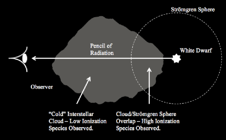
Figure 23: Schematic of Strömgren Sphere interacting with a cloud of gas. Radiation passing through the cloud outside the sphere produces low ionization state absorption features, while radiation passing through the cloud inside the sphere produces high ionization state absorption features.

In the present work, we have identified circumstellar absorption in WD0455-282, and WD2211-495. We have also seen that the velocities of the highly ionized circumstellar components are strikingly similar to those observed in the ISM lines with low ionization states. Furthermore, prior to the present work, circumstellar absorption has only been observed as a single velocity component. Now, for the first time, we have observed circumstellar absorption with multiple velocity components along the line of sight to WD0455-282. These circumstellar velocities are all very similar to the average ISM velocities along the line of sight to WD0455-282. This is, perhaps, the strongest evidence to date that circumstellar absorption arises as a result of Strömgren sphere ionization.

While Strömgren sphere ionization explains how the low and high ionization state lines form, it does not explain where this material comes from. This material could potentially be inherent to the ISM, or could even be inherent to the white dwarf itself, arising from the post RGB pulsations of the object’s progenitor state.

In Dickinson et al. (2012) the authors provide a table of predicted column densities for absorption features arising from Strömgren sphere ionization. These column densities differ depending upon the transition considered. The largest predicted column density occurs for the resonant C iv doublet at 1548 and 1550Å. Unfortunately, the STIS data used in this work stops short of the doublet. Therefore, for future work, it would be useful to obtain high-resolution spectroscopy for WD0455-282 to observe the C iv doublet. If the double component circumstellar feature is real, then this will also be observed in the C iv doublet.

11 Conclusions

We have presented a detailed UV survey of three hot, DA white dwarf stars. Using data obtained with FUSE and HST, we have measured $T_{\mathrm{eff}}$, log $g$, and atmospheric compositions of these objects. In conjunction with measurements from the astrometric satellite Gaia, we have also directly measured the masses, radii, and gravitational redshift velocities of these stars. Upon comparison with the work of B14 we found our measurement of log $g$ (7.60) for WD0621-376 was much larger than the authors’ value (7.22). We tested the sensitivity of our abundance measurements for WD0621-376 to the different log $g$ values, and found the abundance measurements differed greatly for C, N, O, Fe, and Ni ($>30$%). More work needs to be done to understand the reason as to why our log $g$ measurement for WD0621-376 is much larger than that measured by B14.

We considered the question of why the three white dwarfs studied have metals in their atmospheres. To address this question, we compared the observed atmospheric abundances in the three white dwarfs to those predicted by radiative levitation theory as calculated by Ch94/95. We found that the observed Si abundance in all three white dwarfs was larger than predicted by an order of magnitude. We also found that the Fe abundance in WD0621-376 and WD2211-495 was larger than predicted by an order of magnitude. Given that the Ch94/95 abundances constitute a maximum possible supported abundance, this tentatively implies an external origin for metal pollution. However, it is not clear what this origin might be. This is further complicated by the interplay between radiative levitation, and gravitational diffusion. Therefore, to make any definitive progress on this topic, more sophisticated stellar atmospheric modelling including these processes is required.

In addition to our work on the photospheric features in the atmospheres of the three white dwarfs, we also conducted a survey of lines arising from absorption in the ISM. We made an interesting discovery along the line of sight to WD0455-282, where, for the first time, we detected multiple component circumstellar absorption in the Si iii and Si iv resonant lines. We also detected circumstellar absorption along the line of sight to WD2211-495 in the Si iv 1393Å  line. We did not detect a circumstellar feature in the 1402Å  line. Interestingly, we made no detections of any circumstellar absorption along the line of sight to WD0621-376. We also could not detect the resonant Si iii 1206Å  line along the line of sight to this white dwarf. This is in contrast to WD0455-282 and WD2211-495, where we detected very strong Si iii absorption in both cases. This runs contrary to stellar atmosphere model predictions, where Si iii is weakly populated in comparison to Si iv. This implies that the Si iii line can be used as a reliable tracer of circumstellar absorption along the line of sight to hot white dwarf stars.

Appendix A Gaussian parameterisation

To parameterise the non-photospheric absorption features we used a Gaussian profile. Because there can be a large number of absorbers along the line of sight, the profile can often become saturated. We account for this by using the full expression

$$F_{\lambda}=\prod_{i=1}^{N}{F_{i}}=F_{0}\prod_{i=1}^{N}\exp{\left[-P_{0,i}\phi\right]},$$ (7)

where $F_{0}$ is the continuum flux, $P_{0,i}$ is the absorption strength for the $i$th Gaussian profile, and $\phi$ is the normalised Gaussian function. The product is calculated out over $N$ absorption profiles. $\phi$ is then written as

$$\phi_{\lambda}=\frac{1}{P_{1,i}\sqrt{\pi}}\exp\left[-\frac{(\lambda-P_{2,i})^{2}}{P_{1,i}^{2}}\right],$$ (8)

where $P_{1,i}$ is the Doppler width of the $i$th Gaussian, and $P_{2,i}$ is the centroid wavelength of the $i$th Gaussian. Details on the fitting procedure can be found in the text.

References

- Arnaud (1996) Arnaud K. A., 1996, in Jacoby G. H., Barnes J., eds, Astronomical Society of the Pacific Conference Series Vol. 101, Astronomical Data Analysis Software and Systems V. p. 17
- Badnell (2011) Badnell N. R., 2011, Computer Physics Communications, 182, 1528
- Bannister et al. (2003) Bannister N. P., Barstow M. A., Holberg J. B., Brahweiler F. C., 2003, MNRAS, 341, 477
- Barstow et al. (2003) Barstow M. A., Good S. A., Holberg J. B., Hubeny I., Bannister N. P., Bruhweiler F. C., Burleigh M. R., Napiwotzki R., 2003, MNRAS, 341, 870
- Barstow et al. (2014) Barstow M. A., Barstow J. K., Casewell S. L., Holberg J. B., Hubeny I., 2014, MNRAS, 440, 1607
- Bergeron et al. (2011) Bergeron P., et al., 2011, ApJ, 737, 28
- Chayer et al. (2002a) Chayer P., Fontaine G., Wesemael F., 2002a, ApJS, 99, 189
- Chayer et al. (2002b) Chayer P., LeBlanc F., Fontaine G., Wesemael F., Michaud G., Vennes S., 2002b, ApJ, 436, L161
- Chayer et al. (2002c) Chayer P., Vennes S., Pradhan A. K., Thejll P., Beauchamp A., Fontaine G., Wesemael F., 2002c, ApJ, 454, 429
- Croll et al. (2015) Croll B., et al., 2015, ApJ, 836, 82
- Dickinson et al. (2012) Dickinson N. J., Barstow M. A., Hubeny I., 2012, MNRAS, 421, 3222
- Gänsicke et al. (2006) Gänsicke B. T., Marsh T. R., Southworth J., Rebassa-Mansergas A., 2006, Science, 314, 1908
- Gänsicke et al. (2016) Gänsicke B. T., et al., 2016, ApJ, 818, L7
- Gianninas et al. (2010) Gianninas A., Bergeron P., Dupuis J., Ruiz M. T., 2010, ApJ, 720, 581
- Henden et al. (2016) Henden A., Templeton M., Terrell D., Smith T., Levine S., Welch D., 2016, VizieR Online Data Catalog, p. II/336
- Holberg & Bergeron (2006) Holberg J. B., Bergeron P., 2006, AJ, 132, 1221
- Holberg et al. (2002) Holberg J. B., Barstow M. A., Bruhweiler F. C., Cruise A. M., Penny A. J., 2002, ApJ, 497, 935
- Hu et al. (2018) Hu J., et al., 2018, arXiv e-prints
- Hubeny (1988) Hubeny I., 1988, Computer Physics Communications, 52, 103
- Hubeny & Lanz (2002) Hubeny I., Lanz T., 2002, ApJ, 439, 875
- Hubeny & Lanz (2011) Hubeny I., Lanz T., 2011, in Astrophysics Source Code Library, record ascl:1109.022. p. 9022
- Iben & Tutukov (1997) Iben I., Tutukov A., 1997, Skytel, 94, 36
- Kawka & Vennes (2016) Kawka A., Vennes S., 2016, MNRAS, 458, 325
- Koester et al. (2014) Koester D., Gänsicke B. T., Farihi J., 2014, Astronomy & Astrophysics, 566, A34
- Kowalski & Saumon (2006) Kowalski P. M., Saumon D., 2006, ApJ, 651, L137
- Kurucz (1992) Kurucz K., 1992, Revista Mexicana de Astronomia y Astrofisica, 23, 45
- Lallement et al. (2014) Lallement R., Vergely J.-L., Valette B., Puspitarini L., Eyer L., Casagrande L., 2014, A&A, 561, A91
- Landenberger-Schuh (2005) Landenberger-Schuh S., 2005, PhD thesis, Institut für Astronomie und Astrophysik Tuebingen, Sand 1, D-72076 Tuebingen, Germany; Universitätssternwarte Göttingen, Geismarlandstrasse 11, D-37083 Göttingen, Germany <EMAIL>schuh@astro.physik.uni-goettingen.de</EMAIL>, http://adsabs.harvard.edu/abs/2005PhDT.........1L
- Lemke (2003) Lemke M., 2003, Astronomy and Astrophysics Supplement Series, 122, 285
- Manser (2019) Manser C. J., 2019, Science, 364, 66
- Marinoni et al. (2016) Marinoni S., et al., 2016, MNRAS, 462, 3616
- Markwardt (2009) Markwardt C. B., 2009, in Bohlender D. A., Durand D., Dowler P., eds, Astronomical Society of the Pacific Conference Series Vol. 411, Astronomical Data Analysis Software and Systems XVIII. p. 251 (arXiv:0902.2850), http://arxiv.org/abs/0902.2850
- Martin & Baltimore (2012) Martin S., Baltimore D., 2012, Space Telescope Imaging Spectrograph Instrument Handbook for Cycle 21. No. December
- Moos et al. (2002) Moos H. W., et al., 2002, ApJ, 538, L1
- Paquette et al. (2002) Paquette C., Pelletier C., Fontaine G., Michaud G., 2002, ApJS, 61, 197
- Preval et al. (2013) Preval S. P., Barstow M. A., Holberg J. B., Dickinson N. J., 2013, MNRAS, 436, 659
- Preval et al. (2017) Preval S. P., Barstow M. A., Badnell N. R., Hubeny I., Holberg J. B., 2017, MNRAS, 465, 269
- Rappaport et al. (2016) Rappaport S., Gary B. L., Kaye T., Vanderburg A., Croll B., Benni P., Foote J., 2016, MNRAS, 458, 3904
- Redfield & Linsky (2008) Redfield S., Linsky J. L., 2008, ApJ, 673, 283
- Romero et al. (2019) Romero A. D., Kepler S. O., Joyce S. R. G., Lauffer G. R., Córsico A. H., 2019, MNRAS, 484, 2711
- Seaton et al. (2014) Seaton M. J., Yan Y., Mihalas D., Pradhan A. K., 2014, MNRAS, 266, 805
- Stassun & Torres (2018) Stassun K. G., Torres G., 2018, ApJ, 862, 61
- Strömgren (1939) Strömgren B., 1939, ApJ, 89, 526
- Tremblay & Bergeron (2009) Tremblay P. E., Bergeron P., 2009, ApJ, 696, 1755
- Tremblay et al. (2011) Tremblay P. E., Bergeron P., Gianninas A., 2011, ApJ, 730, 128
- Vanderburg et al. (2015) Vanderburg A., et al., 2015, Nature, 526, 546
- Wilson et al. (2016) Wilson D. J., Gänsicke B. T., Farihi J., Koester D., 2016, MNRAS, 459, 3282
- Xu et al. (2014) Xu S., Jura M., Koester D., Klein B., Zuckerman B., 2014, ApJ, 783, 79
- Xu et al. (2016) Xu S., Jura M., Dufour P., Zuckerman B., 2016, ApJ, 816, L22
- Zuckerman et al. (2011) Zuckerman B., Koester D., Dufour P., Melis C., Klein B., Jura M., 2011, ApJ, 739, 101