Self-similar breakup of polymeric threads as described by the Oldroyd-B model

Abstract

When a drop of fluid containing long, flexible polymers breaks up, it forms threads of almost constant thickness, whose size decreases exponentially in time. Using an Oldroyd-B fluid as a model, we show that the thread profile, rescaled by the thread thickness, converges to a similarity solution. Using the correspondence between viscoelastic fluids and non-linear elasticity, we derive similarity equations for the full three-dimensional axisymmetric flow field in the limit that the viscosity of the solvent fluid can be neglected. A conservation law balancing pressure and elastic energy permits to calculate the thread thickness exactly. The explicit form of the velocity and stress fields can be deduced from a solution of the similarity equations. Results are validated by detailed comparison with numerical simulations.

1 Introduction

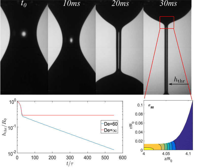
Figure 1: An illustration of the problem studied in this paper. On the top, a sequence of experimental images showing the pinch-off of a drop of polymer solution (PAM) between two solid plates, forming a uniform thread of radius $h_{\rm thr}(t)$ Deblais et al. (2018b). On the bottom, our numerical simulation of the Oldroyd B model for flexible polymer solutions, with dimensionless parameters (defined in Section 2.3), chosen as in Turkoz et al. (2018): ${\rm De}=\lambda/\tau=60$, ${\rm Oh}=3.16$, $S=\eta_{s}/\eta_{0}=0.25$. The elasto-capillary number is $G=\eta_{p}R_{0}/(\lambda\gamma)=0.0395$. Times are made dimensionless with the capillary time scale $\tau=\sqrt{\rho R_{0}^{3}/\gamma}$, and lengths are given in units of the initial bridge radius $R_{0}$. On the left, $h_{\rm thr}(t)$ is shown to decrease exponentially in time, with decay exponent $1/3\lambda$, where $\lambda$ is the polymer timescale (blue line). For comparison, we also include a simulation with infinite relaxation time, keeping $G$ constant. On the right, a closeup of the corner region between the thread and the drop, showing the axial stress $\sigma_{zz}$. The stress is very high inside the thread, and decays very rapidly in the transition region.

When a drop of water falls from a tap, it will break into two or more pieces under the action of surface tension Eggers & Villermaux (2008). Similarly, holding a drop between two solid plates which are then separated to make this liquid bridge unstable, breakup is observed at some finite time $t_{0}$. Near breakup time, drop profiles and the velocity field are characterised by similarity solutions Eggers (1993); Eggers & Fontelos (2015), which describe the evolution toward smaller and smaller scales.

If even a small amount of long, flexible polymer is added, the singularity is inhibited Bazilevskii et al. (1981); Amarouchene et al. (2001); Chang et al. (1999); Clasen et al. (2006); Morrison & Harlen (2010); Eggers & Fontelos (2015), and a thread of almost uniform thickness is formed, as shown in Fig. 1. This is because polymers are stretched in the extensional flow near breakup, but resist the stretching, producing an axial stress, sometimes quantified as an extensional viscosity. This slows down the pinching, and results in a uniform thread thickness. In the framework of the Oldroyd-B model for polymer solutions, the characteristic relaxation time $\lambda$ of the polymer selects a constant extension rate $\dot{\epsilon}$ inside the thread, which leads to an exponential thinning

$$h_{\rm thr}=h_{0}\exp\left(-\frac{t}{3\lambda}\right)$$ (1)

of the thread radius Bazilevskii et al. (1990); Clasen et al. (2006); Eggers & Villermaux (2008). This is well confirmed by experiments Bazilevskii et al. (1990); Anna & McKinley (2001); Amarouchene et al. (2001); Clasen et al. (2006) in both high and low viscosity solvents, as well as in full numerical simulations of the Oldroyd-B equations Etienne et al. (2006); Bhat et al. (2010); Turkoz et al. (2018).

In Fig. 1 (red curve on bottom left) we also show the minimum thread radius for a simulation in which we have taken the limit of infinite relaxation time. As a result, elastic stresses do not relax, and a stationary minimum thread thickness is reached at a point where elastic and surface tension forces balance. Below we will show that the time-dependent problem of an exponentially thinning thread is closely related to the stationary elastic problem. Both are described by the same similarity solution, respectively, in the limit of long times, and of vanishing elasto-capillary number (given that contributions from the solvent are small).

One of the main outstanding questions is to calculate the prefactor $h_{0}$ theoretically, and to relate it to the extensional viscosity inside the thread. By measuring the thread thickness one could then infer the viscosity, and thus use the device as a rheometer Bazilevskii et al. (1990). However, it was pointed out by Clasen et al. (2006) that a proper description of the thread cannot result from a force balance within the uniform thread alone, since the driving force of the motion results from the capillary pressure difference between the thread and the drops which connect to it (cf. sequence at the top of Fig. 1). To calculate the resistive force, one has to consider the flow of liquid emptying from the thread into the drops (of which in Fig. 1 there is one on either end of the thread). As a result, the task is to understand the transition region connecting the thread and the drop, which has the form of a similarity solution Clasen et al. (2006); Turkoz et al. (2018): if both the axial and radial coordinates are rescaled by the thread thickness $h_{\rm thr}$, the drop profile in the corner region connecting the thread and the drop falls onto a universal curve.

In Clasen et al. (2006) the similarity solution for the corner was calculated in the framework of lubrication theory, which is valid if the interface slope is assumed small, so the flow inside the thread can be described within a one-dimensional model. Clearly, this is not satisfied throughout the corner as seen in Fig. 1; we will in fact find that the slope of the similarity solution grows exponentially away from the thread. It is also clear that the stress distribution has a significant radial dependence (cf. the bottom right of Fig. 1), which cannot be captured by a one-dimensional model.

A more recent numerical study Turkoz et al. (2018) has confirmed that the corner solution is fully three-dimensional axisymmetric, while it has the similarity structure anticipated in Clasen et al. (2006). The present paper closes this gap by calculating the full self-similar structure of the three-dimensional axisymmetric equations, both numerically and theoretically. Following many previous papers, we do this in the framework of the Oldroyd-B model, which has become a standard model for the description of solutions of long, flexible polymers Bird et al. (1987); Larson (1999); Morozov & Spagnolie (2015), including capillary flows Eggers & Villermaux (2008). The stress contains contributions from both the polymers themselves, and a Newtonian contribution coming from the solvent. Its main simplifying features are that polymers are modelled with a single characteristic relaxation time of the polymer $\lambda$, and that each polymer strand is assumed infinitely extensible, so that the extensional viscosity can become arbitrarily large.

As a result, the exponential thinning regime described by (1) will continue forever in the Oldroyd-B model, which allows us to focus on this critical part of the pinching dynamics. If finite extensibility of the polymer is taken into account Fontelos & Li (2004); Wagner et al. (2005), as in the so-called FENE-P model Bird et al. (1987), pinching proceeds in a localised fashion, similar to the Newtonian case Renardy (2002); Fontelos & Li (2004). However, this mode of breakup does not appear to be a realistic description of experiment, as instead Oliveira & McKinley (2005); Sattler et al. (2008, 2012) the polymer thread undergoes a spatially periodic instability, in the course of which the highly stressed thread partially relaxes, to form a series of small droplets. This has been called the blistering instability Sattler et al. (2008, 2012), whose theoretical description Eggers (2014) has recently been confirmed experimentally Deblais et al. (2018b).

In this paper, we give the first consistent analysis of polymeric pinching using the full three-dimensional, axisymmetric Oldroyd-B equations. In the next section, we present the Oldroyd-B equations of motion. We use a powerful new code based on mapping the physical domain unto a simple rectangular domain Herrada & Montanero (2016); Deblais et al. (2018a), together with a logarithmic transformation of the polymeric stress tensor Turkoz et al. (2018), in order to study the self-similar structure of the polymeric pinching problem in detail. We find that contrary to previous assumptions, owing to the stress contribution from the solvent, the stress distribution inside the thread has a non-constant radial distribution. This suggests the similarity solution in general is non-universal, and dependent on boundary conditions. However, the contribution from the solvent is often small for realistic parameter values, as measured by a dimensionless parameter $\overline{v}_{0}$ which we identify below. As a result, the main focus of our paper is on calculating the universal similarity solution in the limit of vanishing solvent contribution; the non-universal part comes from the solvent contribution.

In Section 3 we present the similarity equations describing the corner region between the polymer thread and the drop including solvent contributions. Since inertia is found to be subdominant asymptotically, the tension in each cross section is conserved. To solve the similarity equations for vanishing solvent parameter $\overline{v}_{0}$, in Section 4 we consider a related problem in non-linear elasticity: the collapse of a cylinder of elastic material under surface tension. As the elastic bridge deforms, elastic stresses build up and eventually balance surface tension to establish a new stationary equilibrium state. For small elastic modulus $\mu$, a thread of almost uniform thickness is formed, whose radius goes to zero in the limit of vanishing $\mu$. We show that this limit is described by a similarity solution, which is identical to the similarity solution for the time-dependent collapse of a viscoelastic fluid bridge.

Using Lagrangian coordinates with respect to the reference state of a cylindrical elastic bridge, we derive a simplified set of similarity equations for the elastic problem in the limit $\mu\rightarrow 0$. The elastic similarity equations are shown to obey a novel conservation law involving the pressure and the elastic energy, which is closely related to Eshelby’s elastic energy-momentum tensor Eshelby (1975). Physically, it represents invariance of the equations under a relabelling of Lagrangian coordinates.

With the help of this conservation law, we are able to calculate the thickness of the elastic thread, without having to solve the full three-dimensional similarity equations. Remarkably, the result agrees with what was found by us earlier Clasen et al. (2006) using a one-dimensional description, because the description correctly respects the conservation law. However, the spatial structure of the similarity solution is different from what the earlier one-dimensional description predicts. We then solve the similarity equations numerically to yield the self-similar interface profile and the stress distribution in the interior. This then solves the problem both of the time-dependent pinching of a viscoelastic thread, and the collapse of an elastic thread.

In a final discussion, we compare numerical results to our similarity theory, and outline future directions of research.

2 Equations of motion and numerical simulations

The Oldroyd-B model can be described by the following set of equations Bird et al. (1987); Morozov & Spagnolie (2015):

$$\rho\left(\frac{\partial{\bf v}}{\partial t}+\left({\bf v}\cdot{\bm{\nabla}}\right){\bf v}\right)=-{\bm{\nabla}}p+{\bm{\nabla}}\cdot\bm{\sigma}_{p}+\eta_{s}\triangle{\bf v},$$ (2)

$$\frac{\partial\bm{\sigma}_{p}}{\partial t}+\left({\bf v}\cdot{\bm{\nabla}}\right)\bm{\sigma}_{p}=({\bm{\nabla}}{\bf v})^{T}\cdot\bm{\sigma}_{p}+\bm{\sigma}_{p}\cdot({\bm{\nabla}}{\bf v})-\frac{\bm{\sigma}_{p}}{\lambda}+\frac{\eta_{p}}{\lambda}\dot{\bm{\gamma}}$$ (3)

$${\bm{\nabla}}\cdot{\bf v}=0,$$ (4)

where $\dot{\bm{\gamma}}=({\bm{\nabla}}{\bf v})+({\bm{\nabla}}{\bf v})^{T}$ is the rate-of-deformation tensor, and $\rho$ the fluid density. As seen on the right of the momentum equation (2), the total stress on a fluid element is the sum of two contributions, coming from the solvent and from the polymer. The solvent contributes a Newtonian stress, where $\eta_{s}$ the dynamic viscosity of the solvent, while $\bm{\sigma}_{p}$ is the deviatoric part of the polymeric stress.

The Oldroyd-B model can be derived as the continuum version of a solution of non-interacting model polymers, each of which consists of two beads, experiencing Stokes’ drag, and connected by a Hookean spring. Thus on one hand, springs become stretched when beads move apart as described by the flow. On the other hand, the resulting tension in the string contributes to the polymeric stress $\bm{\sigma}_{p}$, described by the equation of motion (3); (4) enshrines incompressibility of the flow.

In the limit of small shear rates (so that polymers are hardly stretched at all), (2)-(4) describe a Newtonian fluid of total dynamic viscosity $\eta_{0}=\eta_{s}+\eta_{p}$; thus $\eta_{p}$ is known as the polymeric contribution to the viscosity. Polymeric stress relaxes at a rate $\lambda$, as seen from the second to last term on the right of (3), while stretching by the flow is described by the first two terms on the right. In particular, in the case of an extensional flow with constant extension rate $\dot{\epsilon}$, the polymeric stress will grow exponentially if $\dot{\epsilon}\lambda>1/2$. This follows from a comparison of the stretching and relaxation terms. We will see below that in fact $\dot{\epsilon}\lambda=2/3$ inside the thread.

From a continuum perspective, the first four terms of (3) are known as the “upper convected derivative”

$$\overset{\triangledown}{\bm{\sigma}}_{p}=\frac{\partial{\bm{\sigma}}_{p}}{\partial t}+\left({\bf v}\cdot{\bm{\nabla}}\right){\bm{\sigma}}_{p}-\left({\bm{\nabla}}{\bf v}\right)^{T}{\bm{\sigma}}_{p}-{\bm{\sigma}}_{p}\left({\bm{\nabla}}{\bf v}\right).$$ (5)

Its form can be derived purely from the requirement that the polymeric stress ought to transform consistently as a covariant tensor Morozov & Spagnolie (2015).

On account of the axisymmetry of the problem, the velocity field can be written ${\bf v}=v_{r}{\bf e}_{r}+v_{z}{\bf e}_{z}$ in cylindrical coordinates, and the polymeric stress tensor is $\bm{\sigma}_{p}=\sigma_{rr}{\bf e}_{r}\otimes{\bf e}_{r}+\sigma_{rz}{\bf e}_{r}\otimes{\bf e}_{z}+\sigma_{zz}{\bf e}_{z}\otimes{\bf e}_{z}+\sigma_{\theta\theta}{\bf e}_{\theta}\otimes{\bf e}_{\theta}$. The stress boundary condition at the free surface is

$${\bf n}\cdot(\bm{\sigma}_{p}+\eta_{s}\dot{\bm{\gamma}})=(p-\gamma\kappa){\bf n},$$ (6)

where

$$\kappa=\frac{1}{h(1+h_{z}^{2})^{1/2}}-\frac{h_{zz}}{(1+h_{z}^{2})^{\frac{3}{2}}},\quad{\bf n}=\frac{{\bf e}_{r}-{\bf e}_{z}h_{z}}{(1+h_{z}^{2})^{1/2}}$$ (7)

are (twice) the mean curvature and the surface normal, respectively. The coefficient $\gamma$ is the surface tension. If $h(z,t)$ is the thread profile, the kinematic boundary condition becomes

$$\frac{\partial h}{\partial t}+v_{z}(z,h)\frac{\partial h}{\partial z}=v_{r}(z,h).$$ (8)

The numerical problem of solving (2)-(4) with boundary conditions (6) and (8) under conditions of breakup is highly demanding, for a number of reasons. First, the Oldroyd-B equation is well known to exhibit numerical instabilities (for reasons which are not well understood) if $\dot{\epsilon}\lambda$ is of order unity Fattal & Kupferman (2004). This is sometimes known as the high Weissenberg number problem (HWNP). Second, it is crucial to correctly describe the balance between surface tension forces and the force exerted by the polymer, both of which go to zero in the limit of vanishing thread thickness.

2.1 Logarithmic transformation

In order to avoid the HWNP as $\dot{\epsilon}\lambda$ is of order unity, a partial (2D) matrix-logarithm transformation of the polymeric stress tensor $\bm{\sigma}_{p}$ is applied in this work Fattal & Kupferman (2004); Turkoz et al. (2018). The idea behind these transformations is to replace (3), which allows to advance the stresses $\sigma_{rr}$, $\sigma_{zz}$ and $\sigma_{rz}$ in time, with three equations for the elements of a 2x2 symmetric positive-definite matrix $\bm{\psi}$. The first step is to decompose this matrix as

$$\bm{\psi}=\left(\begin{array}[]{ccc}\psi_{zz}&\psi_{rz}\\ \psi_{rz}&\psi_{rr}\end{array}\right)=\mathbf{R}\left(\begin{array}[]{cc}\ln(\Lambda_{1})&0\\ 0&\ln(\Lambda_{2})\\ \end{array}\right)\mathbf{R}^{T},$$ (9)

$\ln(\Lambda_{1})$ and $\ln(\Lambda_{2})$ being the eigenvalues of $\bm{\psi}$, and the columns of $\mathbf{R}$ containing their normalised eigenvectors: $\mathbf{R}\mathbf{R}^{T}=\mathbf{I}$. The second step is to construct the conformation tensor $\mathbf{A}$:

$$\mathbf{A}=\left(\begin{array}[]{cc}A_{zz}&A_{rz}\\ A_{rz}&A_{rr}\\ \end{array}\right)=\mathbf{R}\left(\begin{array}[]{cc}\Lambda_{1}&0\\ 0&\Lambda_{2}\\ \end{array}\right)\mathbf{R}^{T}.$$ (10)

Then, the stresses $\sigma_{zz}$, $\sigma_{rz}$ and $\sigma_{rr}$ can be expressed as function of the elements of $\bm{\psi}$ with the help of $\mathbf{A}$:

$$\sigma_{zz}=\eta_{p}(A_{zz}-1)/\lambda,\quad\sigma_{rr}=\eta_{p}(A_{rr}-1)/\lambda,\quad\sigma_{rz}=\eta_{p}A_{rz}/\lambda.$$ (11)

Finally, the equation of motion for $\bm{\psi}$ is

$$\frac{\partial\bm{\psi}}{\partial t}+(\bm{v}\cdot{\bm{\nabla}})\bm{\psi}-(\bm{\Omega}\bm{\psi}-\bm{\psi}\bm{\Omega})-2\mathbf{B}=\frac{1}{\lambda}\left[\bm{A}^{-1}-\mathbf{I}\right],$$ (12)

with matrices $\bm{\Omega}$, $\bm{B}$ given by

$$\bm{\Omega}=\mathbf{R}\left(\begin{array}[]{cc}0&\omega\\ -\omega&0\\ \end{array}\right)\mathbf{R}^{T},\quad\mathbf{B}=\mathbf{R}\left(\begin{array}[]{cc}M_{11}&0\\ 0&M_{22}\\ \end{array}\right)\mathbf{R}^{T}.$$ (13)

Here

$$\mathbf{M}=\left(\begin{array}[]{cc}M_{11}&M_{12}\\ M_{12}&M_{22}\\ \end{array}\right)=\mathbf{R}^{T}({\bm{\nabla}}\mathbf{v})_{2d}^{T}\mathbf{R},\quad({\bm{\nabla}}\mathbf{v})_{2d}=\left(\begin{array}[]{cc}\frac{\partial v_{z}}{\partial z}&\frac{\partial v_{r}}{\partial z}\\ \frac{\partial v_{z}}{\partial r}&\frac{\partial v_{r}}{\partial r}\\ \end{array}\right),$$ (14)

and $\omega=[\Lambda_{2}M_{12}+M_{21}\Lambda_{1}]/[\Lambda_{2}-\Lambda_{1}]$. In case that $\Lambda_{1}=\Lambda_{2}$, matrices $\bm{\Omega}$, $\bm{B}$ are replaced by

$$\bm{\Omega}=\mathbf{0},\quad\mathbf{B}=\frac{1}{2}[(\mathbf{{\bm{\nabla}}v})_{2d}^{T}+(\mathbf{{\bm{\nabla}}v})_{2d}].$$ (15)

2.2 Mapping technique

The numerical technique used in this study is a variation of that developed in Herrada & Montanero (2016). The spatial physical domain occupied by the fluid is mapped onto a rectangular domain $0\leq\eta\leq 1$, $0\leq\xi\leq L$ by means of the coordinate transformation $\eta=r/h(z,t)$ and $\xi=z$. Then each variable ($v_{z}$, $v_{r}$, $p$, $\psi_{rr}$, $\psi_{rz}$, $\psi_{zz}$, $\sigma_{\theta\theta}$ and $h$) and all its spatial and temporal derivatives, which appear in the transformed equations, are written as a single symbolic vector. For example, seven symbolic elements are associated to the axial velocity, $v_{z}$: $v_{z}$, $\frac{\partial v_{z}}{\partial\eta}$, $\frac{\partial v_{z}}{\partial\xi}$, $\frac{\partial^{2}v_{z}}{\partial^{2}\eta}$, $\frac{\partial^{2}v_{z}}{\partial^{2}\xi}$, $\frac{\partial^{2}v_{z}}{\partial\eta\xi}$, and $\frac{\partial v_{z}}{\partial\tau}$, $\tau=t$ being the transformation for time. The next step is to use a symbolic toolbox to calculate the analytical Jacobians of all the equations with respect to the symbolic vector. Using these analytical Jacobians, we generate functions which can be evaluate later point by point once the transformed domain is discretized in space and time. In this work, we used the MATLAB tool matlabFunction to convert the symbolic Jacobians and equations in MATLAB functions.

Next we carry out the temporal and spatial discretization of the transformed domains. The spatial domain is discretized using a set of $n_{\xi}=850$ equally spaced collocation points in the axial ($\xi$) direction, while a set of $n_{\eta}=20$ of equally spaced collocation points are used in the radial ($\eta$) direction. Fourth-order finite differences are employed to compute the collocation matrices associated with the discretized points. In the time domain, second-order backward finite differences are used for the discretization.

The final step is to solve at each time step the non-linear system of discretized equations using a Newton procedure, where the numerical Jacobian is constructed using the spatial collocations matrices and the saved analytical functions. Since the method is fully implicit, a relatively large fixed time step, $dt/\tau=0.1$, was used in the simulation.

2.3 Numerical results and parameters

As a representative example, we simulate a liquid bridge with periodic boundary conditions, using the parameters of Turkoz et al. (2018). The initial condition is a cylinder of radius $R_{0}$, with a sinusoidal perturbation of small amplitude $\epsilon$ added to it:

$$\frac{h(z,0)}{R_{0}}=1-\epsilon\cos\left(\frac{z}{2R_{0}}\right),\quad-2\pi\leq\frac{z}{R_{0}}\leq 2\pi,$$ (16)

and $\epsilon=0.05$. Only half of the domain was simulated, using symmetry.

We define the dimensionless parameters of the simulation as in Clasen et al. (2006). First, the Deborah number ${\rm De}=\lambda/\tau$ is the dimensionless relaxation time, compared to the capillary time scale $\tau=\sqrt{\rho R_{0}^{3}/\gamma}$. The Ohnesorge number ${\displaystyle{\rm Oh}=\eta_{0}/\sqrt{R_{0}\rho\gamma}}$ measures the relative importance of viscous and inertial effects, while $S=\eta_{s}/\eta_{0}$ is the solvent viscosity ratio. The ratio $\mu=\eta_{p}/\lambda$ defines an elastic constant; it measures the effective shear modulus of the viscoelastic fluid on time scales shorter than the relaxation time $\lambda$. Its dimensionless version

$$G=\mu R_{0}/\gamma=\eta_{p}R_{0}/(\lambda\gamma)$$ (17)

is known as the elasto-capillary number.

In most of the plots shown below, we choose the same parameter values as those in Turkoz et al. (2018): ${\rm De}=60$, ${\rm Oh}=3.16$, $S=\eta_{s}/\eta_{0}=0.25$. The elasto-capillary number is $G=0.0395$. Our mapping technique allows for the description of all fields with high accuracy, avoiding the singular behaviour of the stress near the free surface reported previously Turkoz et al. (2018). The use of the logarithmic transformation described in Section 2.1, together with a fully implicit formulation, allows for superior stability. As a result, we were able to follow the dynamical evolution to well beyond a dimensionless time of $t/\tau=500$. This corresponds to the minimum thread radius being smaller by a factor of 1/4 than in Turkoz et al. (2018).

3 Similarity description

3.1 Solution inside the thread

As shown in Clasen et al. (2006), and illustrated in Fig. 1, there are three different regions involved in this problem: first, a thread of uniform thickness, inside which polymers are highly stretched by an extensional flow of constant extension rate $\dot{\epsilon}$:

$$v_{r}(r,z,t)=-\dot{\epsilon}r/2,\quad v_{z}(r,z,t)=\dot{\epsilon}z.$$ (18)

As a result, using the kinematic boundary condition at the interface, the thread radius behaves as

$$h_{\rm thr}=h_{0}e^{-\dot{\epsilon}t/2}\equiv h_{0}\ell,\quad\ell=e^{-\dot{\epsilon}t/2},$$ (19)

where $h_{0}$ is a constant Second, fluid is injected from the thread into a drop, in which elastic stresses have relaxed almost completely, and the force balance is dominated by capillarity. Third, connecting the thread and the drop is a corner region, the typical size of which is set by the thread thickness, for which we aim to find a similarity description. A typical velocity scale is set by the velocity $v_{0}=\dot{\epsilon}L/2$ at the exit of the thread, based on the linear axial velocity field $v_{z}$ (cf. (18)), and a vanishing velocity at the middle of the thread (on account of symmetry), of total length $L$.

We begin by finding the solution inside the thread, where the radius is assumed uniform, shrinking at an exponential rate, consistent with the incompressible extensional velocity field (18). Owing to translational invariance along the thread, we assume that the polymeric stress is $z$-independent, but allow for an arbitrary dependence in the radial direction. We expect stresses to be of the same magnitude as the capillary pressure, which scales like $\gamma/h_{\rm thr}$. However, since $h_{0}$ is still to be determined, we now introduce the scaling

$$\sigma_{zz}=\frac{\gamma}{R_{0}\ell}\overline{\sigma}_{0}(\overline{r})+C,\quad\overline{r}=\frac{r}{R_{0}\ell},$$ (20)

where $\overline{\sigma}_{0}$ is the dimensionless axial stress inside the thread. Inserting (20) into (3), the axial component of the terms on the left are:

$$\frac{\partial\sigma_{zz}}{\partial t}+v_{r}\frac{\partial\sigma_{zz}}{\partial r}=\frac{\dot{\epsilon}\gamma}{2R_{0}\ell}\overline{\sigma}_{0}+\frac{\dot{\epsilon}\gamma}{2R_{0}\ell}\overline{r}\overline{\sigma}_{0}^{\prime}-\frac{\dot{\epsilon}\gamma}{2R_{0}\ell}\overline{r}\overline{\sigma}_{0}^{\prime}=\frac{\dot{\epsilon}\gamma}{2R_{0}\ell}\overline{\sigma}_{0},$$

and thus the axial component of (3) becomes

$$\frac{\dot{\epsilon}\gamma}{2R_{0}\ell}\overline{\sigma}_{0}=\left(2\dot{\epsilon}-\frac{1}{\lambda}\right)\left(\frac{\gamma\overline{\sigma}_{0}}{R_{0}\ell}+C\right)+\frac{2\dot{\epsilon}\eta_{p}}{\lambda}.$$

For this to be a solution, we have $\dot{\epsilon}=2/(3\lambda)$ Bazilevskii et al. (1990); Entov & Hinch (1997) and $C=-4\eta_{p}/\lambda$, so that the solution in the thread becomes

$$\sigma_{zz}=\frac{\gamma}{R_{0}\ell}\overline{\sigma}_{0}(\overline{r})-\frac{4\eta_{p}}{\lambda}.$$ (21)

Here $\overline{\sigma}_{0}(\overline{r})$ inside the thread can have an arbitrary radial profile, whereas usually a uniform profile has been assumed. The exact form of the profile will be determined by the initial (non-universal) dynamics of the thread. Analysing the other two components in a similar manner, we find to leading order

$$\sigma_{rz}=\frac{\gamma}{R_{0}}\overline{\sigma}_{rz}^{(0)}(\overline{r})\ell^{2},\quad\overline{\sigma}_{rr}=-\frac{2\eta_{p}}{5\lambda}.$$ (22)

Thus inside the thread, the axial stress $\sigma_{zz}$ dominates over the remaining components.

3.2 Similarity solution for the corner region

We now describe the transition region at the end of the thread, assuming that the thread thickness $h_{\rm thr}$ is the only length scale. Again, the ratio $h_{0}/R_{0}$ is still to be determined, so for the similarity description we use $\ell=\exp\{-t/3\lambda\}$ and the length $R_{0}$, so that Thus using $\ell=\exp\{-t/(3\lambda)\}$, we find the similarity description

$$h(z,t)=R_{0}\ell\overline{h}(\overline{z}),\quad p(z,r,t)=\frac{\gamma}{R_{0}\ell}\overline{p}(\overline{z},\overline{r}),\quad{\bf v}(z,r,t)=v_{0}\overline{\bf v}(\overline{z},\overline{r}),\quad\bm{\sigma}(z,r,t)=\frac{\gamma}{R_{0}\ell}\overline{\bm{\sigma}}(\overline{z},\overline{r}),$$ (23)

where $\overline{z}=z/(R_{0}\ell)$ and $\overline{r}=r/(R_{0}\ell)$. Then to leading order as $\ell\rightarrow 0$, the similarity equations become

$$\overline{{\bm{\nabla}}}\overline{p}=\overline{{\bm{\nabla}}}\cdot\overline{\bm{\sigma}}_{p}+\overline{v}_{0}\overline{\triangle}\overline{\bf v},$$ (24)

$$(\overline{\bf v}\cdot\overline{{\bm{\nabla}}})\overline{\bm{\sigma}}_{p}=(\overline{{\bm{\nabla}}}\overline{\bf v})^{T}\cdot\overline{\bm{\sigma}}_{p}+\overline{\bm{\sigma}}_{p}\cdot(\overline{{\bm{\nabla}}}\overline{\bf v})$$ (25)

$$\overline{{\bm{\nabla}}}\cdot\overline{\bf v}=0,$$ (26)

where $\overline{v}_{0}=v_{0}\eta_{s}/\gamma=\eta_{s}L/(3\lambda\gamma)$. The stress boundary condition is:

$${\bf n}\cdot\left(\overline{\bm{\sigma}}_{p}+\overline{v}_{0}\overline{\dot{\bm{\gamma}}}\right)=(\overline{p}-\overline{\kappa}){\bf n}.$$ (27)

The system (24)-(27) does not contain time, but there are matching conditions to be satisfied for $\overline{z}\rightarrow\pm\infty$. For $\overline{z}\rightarrow-\infty$ the solution has to tend toward the thread solution

$$\overline{\bf v}\rightarrow{\bf e}_{z},\quad\overline{h}\rightarrow\overline{h}_{0},\quad\overline{p}\rightarrow 1/\overline{h}_{0},\quad\overline{\bm{\sigma}}_{p}\rightarrow\overline{\sigma}_{0}(\overline{r}){\bf e}_{z}\otimes{\bf e}_{z}.$$ (28)

The first condition says that since the scale of the similarity solution $h_{\rm thr}$ is much smaller than the length $L$ of the thread, the velocity of the similarity solution has to match the velocity at the exit of the thread. The other conditions correspond to thickness and the stress distribution inside the thread. To verify the similarity form (23) we present our numerical results in scaled form in Figures 2 and 3. We indeed observe a collapse of the data and moreover the numerics confirm the matching conditions (28).

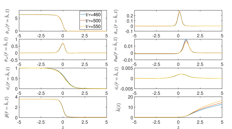
Figure 2: Results of a numerical simulation with parameters as in Fig. 1, rescaled to similarity variables according to (23). The profiles for three different times collapse onto a time-independent similarity solution. The top four profiles are the components of the stress tensor, evaluated at the surface, the bottom four profiles show the components of the velocity, the pressure (again at the surface), as well as the surface profile itself. All profiles collapse onto the time-independent similarity solution defined by (23).

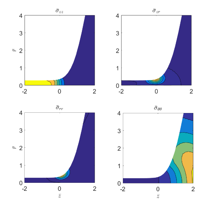
Figure 3: Contour plots of stresses, rescaled according to (23), obtained as in Fig. 2, for the last dimensionless time $t/\tau=550$.

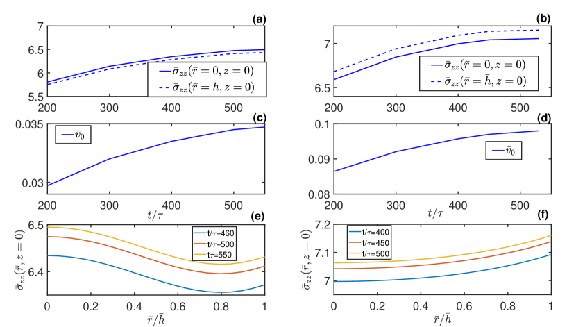
Figure 4: A convergence study of the axial stress distribution inside the uniform thread, taken at the middle of the thread $z=0$. The left hand column (a), (c) and (e) corresponds to $S=\eta_{s}/\eta_{0}=0.25$ as in Fig. 1, the right hand column while (b),(d) and (f) to $S=0.7$; all other parameters are as in Fig. 1. The top two panels demonstrate convergence toward a self-similar stress distribution, which remains non-constant over the radius, as the dimensionless exit velocity converges toward its asymptotic value (two middle panels). The bottom two panels show the self-similar stress profiles $\overline{\sigma}_{0}(\overline{r})$. The shape of the profiles, scaled according to (23), depends on the solvent ratio $S$.

Our main aim will be to calculate the self-similar thread thickness $\overline{h}_{0}$, which determines the prefactor in the exponential thinning law (19). Clearly, $\overline{h}_{0}$ will depend on the initial thread radius: the build-up of elastic tension depends on the history of deformation, and thus must involve the ratio $h_{\rm thr}/R_{0}$. However, in obtaining the similarity description (24)-(25), the choice of the length $R_{0}$ was somewhat arbitrary, in the sense that any fixed length would give rise to the same similarity equations. The effect of the initial jet radius will be properly introduced in Sec.4, where $\overline{h}_{0}$ will be determined. However, the product $h\sigma_{zz}=\gamma\overline{h}_{0}\overline{\sigma}_{zz}$ does not depend on either $R_{0}$ or $\ell$, and is thus expected to be universal. This means that with $\overline{h}_{0}$ in hand and measuring $h$, one can deduce the extensional stress in the thread.

As implied by (21) and (28), the stress will in general not be constant across the fibre, corresponding to a stress distribution $\overline{\sigma}_{0}(\overline{r})$ which depends on the radius explicitly. This is confirmed in Fig. 4, although deviations from a constant stress are small, since the dimensionless exit velocity $\overline{v}_{0}=0.035$ is small. Indeed, we will see below that for $\overline{v}_{0}=0$ the radial stress distribution is uniform. On the top we show the axial stress on the axis and on the surface, which converge to different values in the long-time limit. While for $S=0.25$ the stress is greater on the axis, for $S=0.7$ it is the other way around.

On the bottom we show the corresponding profiles across the thread for the two different values of the solvent viscosity. The two shapes are entirely different, and indicate a non-universal dependence of the stress distribution on the initial dynamics of the collapsing bridge.

3.3 Force balance

Now we derive boundary conditions for $\overline{z}\rightarrow\infty$, i.e. toward the drop. Owing to the scaling of the polymeric stress $\sim 1/h\sim e^{\dot{\epsilon}t/2}$, the total tension inside the thread scales like $\sigma h^{2}\sim\ell\sim e^{-\dot{\epsilon}t/2}$, which needs to be supported by surface tension forces inside the drop Clasen et al. (2006). To derive this more formally, we follow Eggers & Fontelos (2005) and integrate (24), written in the form $\overline{{\bm{\nabla}}}\cdot\left(\overline{\bm{\sigma}}_{p}+\overline{v}_{0}\overline{\dot{\bm{\gamma}}}-p{\bf I}\right)\equiv\overline{{\bm{\nabla}}}\cdot\overline{\bm{\sigma}}=0$, over the fluid volume bounded by the planes $\overline{z}=\overline{z}_{\pm}$. Using the dynamic boundary conditions in the form $\overline{\bf n}\cdot\overline{\bm{\sigma}}=-\overline{\kappa}\overline{\bf n}$, we have

$$0=\oint_{S}\overline{\bf n}\cdot\overline{\bm{\sigma}}ds=-\int_{O}\overline{\kappa}\overline{\bf n}ds\pm\int_{C_{\pm}}{\bf e}_{z}\cdot\overline{\bm{\sigma}},$$ (29)

where $S$ is the closed surface between the planes $\overline{z}=\overline{z}_{+}$ and $\overline{z}=\overline{z}_{-}$, denoted $C\pm$, as well as the jet surface $O$. According to Eggers & Fontelos (2005), the integral over $O$ is

$$\int_{O}\overline{\kappa}\overline{\bf n}ds=-\left.\frac{2\pi\overline{h}}{\sqrt{1+\overline{h}_{\overline{z}}^{2}}}\right|_{\overline{z}_{-}}^{\overline{z}_{+}}{\bf e}_{z},$$

and the integral over the $z$-component of $C_{+}$ and $C_{-}$ is (using incompressibility to transform the viscous term)

$$2\pi\left[\int_{0}^{\overline{h}}\overline{r}\overline{\sigma}^{(p)}_{zz}d\overline{r}-\int_{0}^{\overline{h}}\overline{r}\overline{p}d\overline{r}-2\overline{v}_{0}\overline{h}\overline{v}_{r}(\overline{h},\overline{z})\right]_{\overline{z}_{-}}^{\overline{z}_{+}}.$$

We note further that

$$\frac{2\overline{h}}{\sqrt{1+\overline{h}_{\overline{z}}^{2}}}-2\int_{0}^{\overline{h}}\overline{r}\overline{\kappa}d\overline{r}=\frac{2\overline{h}}{\sqrt{1+\overline{h}_{\overline{z}}^{2}}}-\overline{h}^{2}\kappa=\overline{h}^{2}\overline{K},$$

where

$$K=\frac{1}{h(1+h_{z}^{2})^{1/2}}+\frac{h_{zz}}{(1+h_{z}^{2})^{\frac{3}{2}}},$$ (30)

so that (29) can be written as

$$0=\left.2\int_{0}^{\overline{h}}\overline{r}\overline{\sigma}^{(p)}_{zz}d\overline{r}+2\int_{0}^{\overline{h}}\overline{r}(\overline{\kappa}-\overline{p})d\overline{r}-4\overline{v}_{0}\overline{h}\overline{v}_{r}(\overline{h},\overline{z})+\overline{h}^{2}\overline{K}\right|_{\overline{z}_{-}}^{\overline{z}_{+}}.$$ (31)

So far no approximation has been made.

Using the boundary conditions (28) inside the thread, (31) becomes

$$\overline{T}\equiv\left.2\int_{0}^{\overline{h}_{0}}\overline{r}\overline{\sigma}_{0}(\overline{r})d\overline{r}+\overline{h}_{0}=2\int_{0}^{\overline{h}}\overline{r}\overline{\sigma}^{(p)}_{zz}d\overline{r}+2\int_{0}^{\overline{h}}\overline{r}(\overline{\kappa}-\overline{p})d\overline{r}-4\overline{v}_{0}\overline{h}\overline{v}_{r}(\overline{h},\overline{z})+\overline{h}^{2}\overline{K}\right|_{\overline{z}=\overline{z}_{+}},$$ (32)

where $\pi\overline{T}$ is the constant tension in the liquid thread. As we confirm below, all viscous and elastic stresses decay rapidly inside the drop, and the balance is maintained by surface tension forces alone. As a result, the deviatoric part of the stress $\overline{\sigma}_{zz}$ and $\overline{v}_{r}$ decay rapidly as $\overline{z}\rightarrow\infty$, and the pressure almost equals the capillary pressure: $\overline{p}\approx\overline{\kappa}$. Only the fourth term on the right of (32), coming from surface tension, survives, and equation describing the shape of the capillary region is Eggers & Fontelos (2015):

$$\overline{T}=\overline{h}^{2}\overline{K}.$$ (33)

This equation describes the crossover toward the drop, whose dimensionless radius $\overline{R}=R/h_{\rm thr}$ diverges in the limit. Indeed, in the intermediate region where $\overline{h}\ll\overline{R}$, the only way the right hand side of (33) can be constant is to require that $\overline{h}/\overline{h}_{\overline{z}}\rightarrow const$, which is achieved for

$$\overline{h}=He^{a\overline{z}},\quad\overline{z}\rightarrow\infty.$$ (34)

This means the right hand side of (33) becomes $2/a$ in the limit, and we obtain

$$\overline{T}=\frac{2}{a}.$$

4 The elastic correspondence

At least in the limit that the contribution from the solvent in the momentum balance (24) is negligible, one can make use of the fact that in the similarity equations (24)-(25) terms containing the relaxation time $\lambda$ have disappeared. Thus, we anticipate that the same set of equations can be obtained in a purely elastic description, where we take the limit $\lambda\rightarrow\infty$ such that elastic stress do not relax. In the absence of inertia the elastic equations describe the equilibrium between surface tension, which tends to deform the elastic medium, and elasticity, which resists deformation. Thus for $\lambda\rightarrow\infty$, but keeping $\mu=\eta_{p}/\lambda$ fixed, this equilibrium state is described by

$${\bm{\nabla}}p={\bm{\nabla}}\cdot\bm{\sigma}_{p},$$ (35)

$$\overset{\triangledown}{\bm{\sigma}}_{p}=\mu\dot{\bm{\gamma}},$$ (37)

$${\bm{\nabla}}\cdot{\bf v}=0,$$

using that $\partial_{t}\bm{\sigma}_{p}=0$. One can already see that in the limit of vanishing elasticity $\mu\rightarrow 0$, (35)-(37) are identical to the similarity equation (24)-(25) for the case where $v_{0}=0$ (the stress coming from the solvent can be neglected). So indeed, the similarity solution can be computed from the elastic limit. However, it is advantageous to first retain the elastic term $\mu\dot{\bm{\gamma}}$, as it will allow to properly introduce the history-dependence into the description, and to determine the value of $\bar{h}_{0}$ we are looking for.

To proceed, we first show (for details see Snoeijer et al. (2019)), that instead of solving (37) with the constraint (37), one can write $\bm{\sigma}_{p}$ as the stress tensor of a neo-Hookean elastic solid, which depends quadratically on the deformation from an unstressed reference state. Thus one needs to find a transformation of the undeformed state (e.g. a cylinder), parameterized by variables $R,Z$, into a deformed state $r=r(R,Z),z=z(R,Z)$ such that elastic and surface tension forces are balanced. The equilibrium state is characterised by the deformation tensor (in Cartesians)

$$F_{iK}=\frac{\partial x_{i}}{\partial X_{K}},$$ (38)

which satisfies incompressibility

$$\det{\bf F}=\frac{r}{R}\left(\frac{\partial r}{\partial R}\frac{\partial z}{\partial Z}-\frac{\partial r}{\partial Z}\frac{\partial z}{\partial R}\right)=1.$$ (39)

Here lower case variables and lower case indices refer to the deformed state, upper case variables and upper case indices refer to the undeformed state.

If we write the stress tensor as ${\bm{\sigma}}_{p}=\mu\left({\bf A}-{\bf I}\right)$, where ${\bf A}$ is the conformation tensor as in (11), then (37) simplifies to $\overset{\triangledown}{\bf A}=0$. Using the fact that ${\bf v}=d{\bf x}/dt$, where the time derivative is taken at a constant material point ${\bf X}$, one shows that Morozov & Spagnolie (2015)

$$\overset{\triangledown}{\bf A}={\bf F}\left[\frac{d}{dt}\left({\bf F}^{-1}{\bf A}{\bf F}^{-T}\right)\right]{\bf F}^{T}$$ (40)

From this relation, it is clear that ${\bf A}={\bf F}{\bf F}^{T}$ indeed provides an integral to the equation $\overset{\triangledown}{\bf A}=0$. In addition, this solution satisfies the condition that $\bm{\sigma}_{p}=0$ in the initial configuration, where ${\bf F}={\bf I}$.

With the above steps we have managed to integrate (37), and have identified $\bm{\sigma}_{p}$, satisfying a stress-free initial condition. Since $-\mu{\bf I}$ can be written as part of the pressure $p$, the elastic stress tensor becomes

$$\bm{\sigma}=-p{\bf I}+\bm{\sigma}_{p}\equiv-p{\bf I}+\mu{\bf F}{\bf F}^{T},$$ (41)

which is the classical result for the “true” stress tensor of a new-Hookean solid Suo (2013b, a). Then in terms of the deformation, the stress tensor becomes Negahban (2012)

$$\bm{\sigma}_{p}=\mu\begin{pmatrix}\left(\frac{\partial r}{\partial R}\right)^{2}+\left(\frac{\partial r}{\partial Z}\right)^{2}&0&\frac{\partial r}{\partial R}\frac{\partial z}{\partial R}+\frac{\partial r}{\partial Z}\frac{\partial z}{\partial Z}\\ 0&\left(\frac{r}{R}\right)^{2}&0\\ \frac{\partial r}{\partial R}\frac{\partial z}{\partial R}+\frac{\partial r}{\partial Z}\frac{\partial z}{\partial Z}&0&\left(\frac{\partial z}{\partial Z}\right)^{2}+\left(\frac{\partial z}{\partial R}\right)^{2}\end{pmatrix}.$$ (42)

The true elastic stress is formulated in the deformed state, (just like the fluid stress tensor), and thus satisfies the same equilibrium conditions as before, but with $v_{s}=0$:

$${\bm{\nabla}}\cdot\bm{\sigma}=0,\quad\left.{\bf n}\cdot\bm{\sigma}_{p}\right|_{S}=\gamma(p-\kappa){\bf n}.$$ (43)

If $R_{0}$ is the radius of the unperturbed interface as usual, the free surface $h(z)$ has the parametric representation

$$h(z(R_{0},Z))=r(R_{0},Z).$$ (44)

Transforming the equilibrium condition (43) to Lagrangian coordinates, we obtain in cylindrical coordinates:

$$\frac{\mu R}{r}\left[\frac{\partial^{2}r}{\partial R^{2}}+\frac{1}{R}\frac{\partial r}{\partial R}-\frac{r}{R^{2}}+\frac{\partial^{2}r}{\partial Z^{2}}\right]=\frac{\partial p}{\partial R}\frac{\partial z}{\partial Z}-\frac{\partial p}{\partial Z}\frac{\partial z}{\partial R},$$ (45)

$$\frac{\mu R}{r}\left[\frac{\partial^{2}z}{\partial R^{2}}+\frac{1}{R}\frac{\partial z}{\partial R}+\frac{\partial^{2}z}{\partial Z^{2}}\right]=\frac{\partial p}{\partial Z}\frac{\partial r}{\partial R}-\frac{\partial p}{\partial R}\frac{\partial r}{\partial Z},$$ (46)

for the radial and axial force balances, respectively. The stress boundary conditions on the surface are

$$-\left.\frac{h_{z}^{2}\sigma_{zz}-2h_{z}\sigma_{rz}+\sigma_{rr}}{1+h_{z}^{2}}=\gamma(\kappa-p)\right|_{r=h},$$ (47)

$$\left.h_{z}(\sigma_{rr}-\sigma_{zz})+(1-h_{z}^{2})\sigma_{rz}=0\right|_{r=h}.$$ (48)

4.1 Elastic similarity equations

We now analyse the elastic problem in the limit $G=\mu R_{0}/\gamma\rightarrow 0$, which corresponds to the similarity solution for the pinching of a polymeric thread. We expect a static balance between elastic stresses and surface tension to be established at a thread thickness which scales like an elasto-capillary length scale $\ell_{e}$: $z\propto r\propto\ell_{e}$. Here we have anticipated that as in the similarity solution (23), both Eulerian coordinates scale in the same way. By contrast, the Lagrangian coordinates do not have the same scales for $R$ and $Z$. Namely, the radial coordinate $R$ must be rescaled by the original radius $R_{0}$; on account of incompressibility (39) we have that $Z\propto\ell_{e}^{3}/R_{0}^{2}$. This implies that the $d/dZ\gg d/dR$, so that the dominant stress contributions in (42) is of the order $\bm{\sigma}_{p}\propto\mu R_{0}^{4}/\ell_{e}^{4}$. The curvature $\kappa$ scales as the inverse radius $h^{-1}\propto\ell_{e}^{-1}$ of the thread (cf. (7)), and thus on account of the stress balance (43) $\mu R_{0}^{4}/\ell_{e}^{4}\propto\gamma/\ell_{e}$. As a result, the elasto-capillary length scale becomes

$$\ell_{e}=\left(\frac{\mu R_{0}^{4}}{\gamma}\right)^{1/3}=R_{0}G^{1/3},$$ (49)

which sets the thickness of the thread Eggers & Fontelos (2015), at which elastic and capillary forces are balanced.

According to the scaling analysis above, we introduce the similarity solution

$$z=\ell_{e}\phi(\overline{R},\overline{Z}),\quad r=\ell_{e}\psi(\overline{R},\overline{Z}),\quad p=(\gamma/\ell_{e})\Pi(\overline{R},\overline{Z}),$$ (50)

valid in the limit $G\rightarrow 0$, where $\overline{R}=R/R_{0}$ and $\overline{Z}=ZR_{0}^{2}/\ell_{e}^{3}$. The rescaled thread thickness $\overline{h}$ is defined by $h=G^{1/3}\overline{h}$, and $z=\ell_{e}\overline{z}$, so the slope $h_{z}=\overline{h}_{\overline{z}}$ remains invariant under the scalings, and $h_{zz}=\ell^{-1}\overline{h}_{\overline{z}\overline{z}}$. As a result, the curvature scales as $\kappa=\ell^{-1}\overline{\kappa}$, where $\overline{\kappa}$ is defined as in (7), but on the basis of $\overline{h}(\overline{z})$. Note that with this scaling, $\bm{\sigma}_{p}\propto\mu G^{-4/3}$, so that the right hand side of (37) becomes subdominant in the limit. As a result, the elastic similarity equations defined by the above rescaling become identical to (24)-(25) in the limit that solvent effects are negligible ($v_{0}=0$), and the similarity profiles (overlined variables defined above) are the similarity profiles defined by (23) in that limit. The only way $\mu$ still enters into the problem is through the initial condition, for which we require that the conformation tensor ${\bf A}={\bf I}$. The rescaling (23), on the other hand, still contains a free length scale $R_{0}$, which we choose such that the similarity profiles of both the time-dependent problem and of the elastic problem are the same.

The key observation is that the ratio $G=(\ell_{e}/R_{0})^{3}$ between a characteristic axial scale and a radial scale in Lagrangian coordinates becomes very small in the limit. As a result, radial derivatives can be neglected relative to axial ones. It also means that in the limit $G\rightarrow 0$ fluid elements become stretched out in the axial direction, so that the self-similar region comes from just a single point in the reference configuration. The radius $R_{0}$ has to be taken as the radius at that point in the reference configuration.

With the scalings (50), the similarity equations become, beginning with incompressibility,

$$\frac{\psi}{\overline{R}}\left(\psi_{\overline{R}}\phi_{\overline{Z}}-\psi_{\overline{Z}}\phi_{\overline{R}}\right)=1.$$ (51)

The equilibrium conditions (45) and (46) are, to leading order as $G\rightarrow 0$,

$$\frac{\overline{R}}{\psi}\psi_{\overline{Z}\overline{Z}}=\Pi_{\overline{R}}\phi_{\overline{Z}}-\Pi_{\overline{Z}}\phi_{\overline{R}},\quad\frac{\overline{R}}{\psi}\phi_{\overline{Z}\overline{Z}}=\Pi_{\overline{Z}}\psi_{\overline{R}}-\Pi_{\overline{R}}\psi_{\overline{Z}}.$$ (52)

The key point is that the second radial derivatives on the right hand side have disappeared, and as result the equations are of first order only in the radial coordinates.

The deviatoric stresses are at leading order

$$\sigma_{zz}=\frac{\gamma}{\ell_{e}}\phi_{\overline{Z}}^{2},\quad\sigma_{rz}=\frac{\gamma}{\ell_{e}}\phi_{\overline{Z}}\psi_{\overline{Z}},\quad\sigma_{rr}=\frac{\gamma}{\ell_{e}}\psi_{\overline{Z}}^{2},$$ (53)

and so the boundary conditions (47),(48), to be evaluated at the surface $\overline{R}=1$, become to leading order

$$-\frac{h_{z}^{2}\phi_{\overline{Z}}^{2}-2h_{z}\phi_{\overline{Z}}\psi_{\overline{Z}}+\psi_{\overline{Z}}^{2}}{1+h_{z}^{2}}=\overline{\kappa}-\Pi,$$ (54)

$$h_{z}\left(\psi_{\overline{Z}}^{2}-\phi_{\overline{Z}}^{2}\right)+(1-h_{z}^{2})\phi_{\overline{Z}}\psi_{\overline{Z}}=0.$$ (55)

But along the surface we have

$$\left.\frac{\psi_{\overline{Z}}}{\phi_{\overline{Z}}}\right|_{R=1}=\left.\frac{\partial r}{\partial z}\right|_{R=1}=h_{z},$$

and so dividing through (54) and (55) by $\phi_{\overline{Z}}^{2}$, the left hand side of both equations is seen to vanish. As a result, the tangential stress balance (55) is satisfied identically in the limit $G\rightarrow 0$, while the kinematic boundary condition as well as the normal stress balance become

$$\psi(1,\overline{Z})=\overline{h}(\phi(1,\overline{Z})),\quad\Pi(1,\overline{Z})=\overline{\kappa}.$$ (56)

Thus as (52) is only of first order in $\overline{R}$, there is only one stress boundary condition to be satisfied instead of two.

We now show that the pressure may be eliminated from the leading-order equations. Multiplying the first equation of (52) by $\phi_{\overline{Z}}$ and using (51), we find

$$\phi_{\overline{Z}}\phi_{\overline{Z}\overline{Z}}=\Pi_{\overline{Z}}+\frac{\psi}{R}\psi_{\overline{Z}}\left(\Pi_{\overline{Z}}\phi_{R}-\Pi_{R}\phi_{\overline{Z}}\right)=\Pi_{\overline{Z}}-\psi_{\overline{Z}}\psi_{\overline{Z}\overline{Z}},$$

using the second equation (52) in the second step. This can be integrated over $\overline{Z}$ to

$$\frac{1}{2}\left(\phi_{\overline{Z}}^{2}+\psi_{\overline{Z}}^{2}\right)=\Pi+C,$$ (57)

where the constant of integration $C$ is in general still a function of $\overline{R}$. In our particular case, we will see that in fact $C=0$. The conservation law expressed by (57) can be shown to be a special case of conservation laws discovered by Eshelby (1975).

4.2 Numerical simulations of the elastic equations

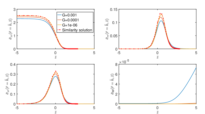
Figure 5: Convergence of the elastic solution toward the similarity solution (50) for smaller and smaller values of the dimensionless elasto-capillary number $G=\mu R_{0}/\gamma$. Stresses have been rescaled according to (59). Profiles from the similarity solution as described in Section 4.4 are shown as the dashed line for comparison.

Before we continue with solving the similarity equations, we test the similarity ansatz (50) by rescaling full numerical simulations of the elastic equations (41)-(44). For the numerical treatment, we define the reference state by

$$R=R_{0}(Z)\eta,\quad Z=Z_{0}(\xi),$$

with the elastic domain defined by $\eta\in[0,1]$ and $\xi\in[0,1]$ The function $Z_{0}(\xi)$ is designed to ensure a homogeneous distribution of grid points in the deformed state, starting from a uniform $\xi$-grid. This accounts for the extreme stretching in the $Z$-direction for small values of $G$, and ensures that enough points remain in the corner region.

As an initial condition, we take the free surface shape

$$h_{\rm in}(z)=1-\epsilon\cos(z/2),$$ (58)

where $\epsilon=0.005$. We are looking for two unknown functions $f$ and $g$, where $r=r(R,Z)=f(\eta,\xi)$ and $z=z(R,Z)=g(\eta,\xi)$, as well as the pressure $p(\eta,\xi)$. These three unknowns are found from solving the three equations (39) and (43). The free surface $h(z)$ then is given by the parametric representation $h(g(1,\xi))=f_{1}(1,\xi)$, from which the curvature $\kappa$ can be evaluated.

The domain is discretized using fourth-order finite differences with 11 equally spaced points in the $\eta$-direction and 4001 points in the $\xi$-direction. The resulting system of non linear equations is solved using a Newton-Raphson technique Herrada & Montanero (2016). We start from the reference state as an initial guess and $G$ sufficiently large ($G=100$) to ensure the convergence of the Newton-Raphson iterations. Once we get a solution, we use this solution in a new run with a smaller value of $G$. As seen in Fig. 5, rescaled stresses as defined by

$$\overline{\bm{\sigma}}=\frac{\gamma}{\ell_{e}}\bm{\sigma}$$ (59)

converge nicely onto a universal similarity solution.

4.3 The thread thickness

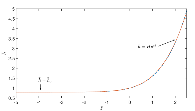
Figure 6: The interface $\overline{h}(\overline{z})$ in similarity variables. The solid line is the rescaled profile obtained from the simulation for $G=10^{-6}$, the dashed line is the solution to the similarity equations. The thread thickness is $\overline{h}_{0}$; for large arguments the profile grows exponentially.

In solving the similarity equations, we first concentrate on the free surface profile, shown in Figure 6 as a real-space profile in similarity variables. We now show that the dimensionless minimum thread thickness $\overline{h}_{0}$ can in fact be calculated without first solving the full similarity equations. Inside the thread, a cylinder of constant dimensionless thickness $\overline{R}=1$ (the reference state) is transformed into a thread whose thickness $\overline{h}_{0}$ is constant. This results in the transformation $\psi=\overline{h}_{0}\overline{R}$, and thus from incompressibility (cf. (51)) $\phi_{\overline{Z}}=1/\overline{h}_{0}^{2}$. Then using (42), the extensional part of the axial stress becomes $\overline{\sigma}_{0}=\phi_{\overline{Z}}^{2}=1/\overline{h}_{0}^{4}$. In particular, the radial stress profile $\overline{\sigma}_{0}(\overline{r})$ of Section 3 is uniform. Since in the elastic case there is no contribution from the velocity, (32) becomes

$$\overline{T}=2\int_{0}^{\overline{h}}\overline{r}\overline{\sigma}_{zz}d\overline{r}+2\int_{0}^{\overline{h}}\overline{r}(\overline{\kappa}-\Pi)d\overline{r}+\overline{h}^{2}\overline{K}.$$ (60)

Evaluating (60) inside the thread of constant thickness, one obtains a finite tension:

$$\overline{T}=\overline{h}_{0}^{2}/\overline{h}_{0}^{4}+\overline{h}_{0}=\overline{h}_{0}+\frac{1}{\overline{h}_{0}^{2}}>0.$$ (61)

This corresponds to the earlier conclusion that there must be a positive tension in a liquid bridge (polymeric or Newtonian) in order for pinching to occur Eggers & Fontelos (2005); Clasen et al. (2006).

On the other hand, toward the “drop” side of the elastic bridge, where $\overline{h}$ becomes large, elastic stresses decay rapidly, as is confirmed by our numerics. As a result, the balance (60) is between $\overline{T}$ and the second term on the left, which must approach a constant. As a result, it follows that for large $\overline{z}$, the similarity profile must be of the form

$$\overline{h}=He^{a\overline{z}},\quad a=\frac{2}{\overline{T}}=\frac{2\overline{h}_{0}^{2}}{1+\overline{h}_{0}^{3}}.$$ (62)

Using (62), both radial and axial contributions to the mean curvature (7) scale like $e^{-2a\overline{z}}$, and cancel to leading order, resulting in $\overline{\kappa}\sim e^{-4a\overline{z}}$. The prefactor $H$ can be normalised to unity by shifting the coordinate system. Thus putting $H=1$ is a way of fixing the origin, ensuring a unique solution.

Applying the conservation law (57) to the thread surface $\overline{R}=1$, we have $\Pi=\overline{\kappa}$, and thus

$$\left.\frac{1}{2}\left(\phi_{\overline{Z}}^{2}+\psi_{\overline{Z}}^{2}\right)\right|_{\overline{R}=1}=\overline{\kappa}+C.$$ (63)

The left hand side is the same as ${\rm tr}\left(\overline{\bm{\sigma}}\right)/2$, which vanishes in the limit $\overline{z}\rightarrow\infty$. Since the curvature vanishes as well for $\overline{z}\rightarrow\infty$, we have $C=0$. On the other hand, for $\overline{z}\rightarrow-\infty$, $\phi_{\overline{Z}}=1/\overline{h}_{0}^{2}$ and $\psi_{\overline{Z}}=0$, while $\overline{\kappa}=1/\overline{h}_{0}$. As a result, (63) yields $1/(2\overline{h}_{0}^{4})=1/\overline{h}_{0}$, and in summary

$$\overline{h}_{0}=2^{-1/3},\quad\overline{\sigma}_{0}=2^{4/3},\quad\overline{T}=\frac{3}{2^{1/3}},\quad a=\frac{2^{4/3}}{3}.$$ (64)

Thus we have calculated the dimensionless thread thickness without explicitly solving the similarity equations. Remarkably, these results are identical to those found using lubrication theory Entov & Yarin (1984); Clasen et al. (2006); Eggers & Fontelos (2015), although the similarity solution doesn’t satisfy the slenderness (small slopes) requirement for lubrication to be valid. The reason is that (64) only relies on the conservation laws (63) and (60), which are preserved in the lubrication limit.

4.4 The similarity solution

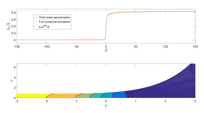
Figure 7: Convergence onto the similarity solution. On the top, the ratio $\overline{h}_{\overline{z}}/\overline{h}$ approaches the limit $a=2^{4/3}/3$, over a wide range of $\overline{Z}$. On the bottom, we show contours of the function $\Pi$ in the $[\phi,\psi]$ domain, showing the transition region between the thread and the drop region. Red dashes lines correspond with contours obtained rescaling the pressure in the elastic simulation with $G=10^{-6}$. Although the radial dependence is weak, the profile is not one-dimensional.

It remains to calculate the actual form of the profile and of the deformation field inside. We can eliminate $\Pi$ from (52), which yields after simplification using (51)

$$\phi_{\overline{R}}\phi_{\overline{Z}\overline{Z}}+\psi_{\overline{R}}\psi_{\overline{Z}\overline{Z}}=\phi_{\overline{Z}}\phi_{\overline{Z}\overline{R}}+\psi_{\overline{Z}}\psi_{\overline{Z}\overline{R}}.$$ (65)

This can be solved together with the incompressibility constraint (51):

$$\psi\left(\psi_{\overline{R}}\phi_{\overline{Z}}-\psi_{\overline{Z}}\phi_{\overline{R}}\right)=\overline{R}.$$

On the surface $\overline{R}=1$, we have (56), which in view of (63) takes the form

$$\psi(1,\overline{Z})=\overline{h}(\phi(1,\overline{Z})),\quad\left.\frac{1}{2}\left(\phi_{\overline{Z}}^{2}+\psi_{\overline{Z}}^{2}\right)\right|_{R=1}=\overline{\kappa}.$$ (66)

Differentiating the first equation of (66), it follows at constant $\overline{R}=1$ that $\psi_{\overline{Z}}=\phi_{\overline{Z}}\overline{h}_{\overline{z}}$, and hence the second equation can also be rewritten

$$\frac{1}{2}\phi_{\overline{Z}}^{2}(1,\overline{Z})=\frac{\overline{\kappa}}{1+\overline{h}_{\overline{z}}^{2}}.$$ (67)

For $\overline{Z}\rightarrow-\infty$ the boundary condition is

$$\psi=2^{-1/3}\overline{R},\quad\phi_{\overline{Z}}=2^{2/3},$$ (68)

clearly there can be an arbitrary shift in $\overline{Z}$. For $\overline{Z}\rightarrow\infty$ we must have

$$h=\psi(\overline{R}=1,\overline{Z})=e^{a\phi(\overline{R}=1,\overline{Z})},$$ (69)

where the prefactor has been chosen $H=1$. For the other elastic fields the boundary condition is that the pressure and all the elastic stresses decay for $\overline{Z}\rightarrow\infty$.

To obtain the similarity solution numerically, the domain $[-L\leq\bar{Z}\leq L]\times[0\leq\bar{R}\leq 1]$ was discretized using $n_{\bar{R}}$ and $n_{\bar{Z}}$ Chebyshev collocation points in the $\bar{R}$ and $\bar{Z}$ directions, respectively. Here $L$ is the value at which the $\bar{Z}$ coordinate is truncated. Since strong axial gradients are expected near the origin $\bar{Z}=0$ the grid is stretched around that location using the stretching function

$$\bar{Z}=L\frac{\operatorname{arctanh}(\beta s)}{\operatorname{arctanh}(\beta)}.$$ (70)

Here $s$ is in the original Chebyshev interval $(-1\leq s\leq 1)$, and $\beta$ a stretching parameter.

Equations (51) and (52) with boundary conditions given by (66) and (68) are discretized in the numerical domain. At $\bar{Z}=L$, the soft boundary condition $\phi_{\bar{Z}\bar{Z}}=\psi_{\bar{Z}\bar{Z}}=0$ is used. The resulting discrete system of nonlinear equations have been solved using the MATLAB function fsolve. As an initial guess for the nonlinear solver, the numerical solution for the elastic simulation with $G=1\times 10^{-6}$, rescaled and interpolated into the similarity mesh was used. Results presented have been obtained using $n_{\bar{R}}=5$, $n_{\bar{Z}}=450$ , $\beta=0.995$ and $L=150$. A larger computational domain by imposing a $L>150$ does not alter the results.

The resulting similarity profiles are shown in Figs. 5-7. In Fig. 5 we compare representative stress profiles obtained from solutions of the elastic problem with those calculated from the similarity solution, in Fig. 6 the profile $\overline{h}(\overline{z})$ is compared in greater detail. In Fig. 7 (top) we show that the solution to the similarity equations has converged in a large domain, using two different methods. In particular, according to (34) and (64) $\overline{h}_{\overline{z}}$ converges to $a=2^{4/3}/3$, as confirmed in Fig. 7.

Apart from a full numerical solution of the two-dimensional similarity equations, we also show the result of a different method of solution, explained in more detail in Appendix B. In view of the weak radial dependence, we expand the solution into a power series (77) in the radial direction. The results of both methods of solution agree very well. On the bottom of Fig. 7, we show contours of the self-similar pressure $\Pi$ in the $[\phi,\psi]$ domain. Once more, agreement with contours obtained by rescaling the simulation for $G=10^{-6}$ agree very well with the full similarity solution.

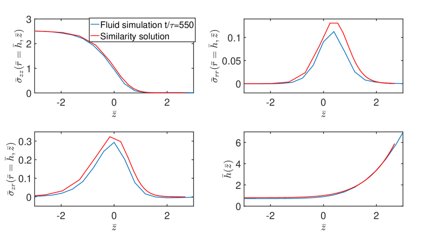
Figure 8: Comparison of the similarity solution as described in Section 4.4 with the rescaled profiles (23) obtained from the time-dependent simulation shown in Fig.1 for ${\rm De}=60$. The time-dependent simulation has been rescaled according to (23), with an effective $R_{0}$ chosen such that $\overline{\sigma}_{zz}=2^{4/3}$ inside the thread.

As a final check, we return to the original problem of the exponential thinning of a viscoelastic liquid bridge, as shown in Fig. 8. Since the dimensionless speed $\overline{v}_{0}=0.035$ is small for our simulations, solvent corrections are expected to be small. Indeed, there is good agreement between our similarity theory based on elastic effects alone, and the full viscoelastic simulations. As we reiterate in the discussion below, there is fading memory in the viscoelastic simulation, and hence there is one adjustable parameter in the comparison, which we choose so that $\overline{\sigma}_{zz}=2^{4/3}$ inside the thread; $\overline{h}=2/\overline{\sigma}_{zz}$ is then predicted without adjustable parameters. This is an effect of ${\rm De}$ being finite; for the value of ${\rm De}=60$ being used in the present simulation, relaxation effects are almost negligible, as discussed below.

5 Discussion

The aim of this paper has been to find similarity solutions describing the time-dependent pinch-off of a polymeric thread. In the process, we found that this similarity solution also describes another problem, the collapse of a soft elastic bridge under surface tension. This fact had been noticed before Clasen et al. (2006), but is generalised here to the full axisymmetric equations. In doing so, we make use of the very general correspondence between fluid flow and non-linear elasticity Snoeijer et al. (2019).

A particular use of our theory is that we can now calculate the radius of the thread that has formed in the middle of the collapsed bridge. In the purely elastic case, returning to dimensional variables, (64) implies that the thread thickness is

$$h_{\rm thr}=R_{0}\left(\frac{G}{2}\right)^{1/3},$$ (71)

where $R_{0}$ is the initial radius of the elastic bridge. In the case of very long relaxation times $\lambda$, such that an initial thread is formed without the polymer having a chance to relax, followed by exponential relaxation in the limit of long times, (71) can be combined with (1) to give Clasen et al. (2006) $h_{0}=R_{0}(G/2)^{1/3}$, and so

$$h_{\rm thr}=R_{0}\left(\frac{G}{2}\right)^{1/3}\exp\left(-\frac{t}{3\lambda}\right),\quad{\rm De}\gg 1.$$ (72)

This is illustrated in the lower left panel of Fig. (1), where the thread radius is shown for ${\rm De}=60$ and for ${\rm De}=\infty$, such that no relaxation takes place. The initial evolution is almost identical for the two case, and the thread radius at the beginning of the exponential relaxation (blue line) is just slightly below the asymptotic value without any relaxation at all (red line).

If however the Deborah number is intermediate, relaxation will take place during formation of the thread, and the prefactor $h_{0}$ will depend on the details of the initial dynamics. However, if one measures the radius $h_{\rm thr}$ of the thread during exponential thinning, the extensional stress can be deduced from it using (64):

$$\sigma_{zz}=\frac{2\gamma}{h_{\rm thr}}.$$ (73)

This relation is needed for the original use of the liquid bridge geometry as a rheometer Bazilevskii et al. (1990): measuring the thread thickness, one can measure the extensional viscosity $\eta_{E}=\sigma_{zz}/\dot{\epsilon}$ Amarouchene et al. (2001).

The present work provides one of the first examples of a similarity solution in three dimensions, which does not reduce to an effective one-dimensional theory Chen & Steen (1997); Day et al. (1998); Eggers (2018). It is to be expected that non-trivial similarity solutions in higher dimensions abound, but not many have been found, owing to technical difficulties in obtaining them. Another, and perhaps related feature concerns the universality of similarity solutions. In a one-dimensional approximation, and taking into account effects of the solvent viscosity, one obtains similarity solutions which depend on the value of the parameter $\overline{v}_{0}$ alone Clasen et al. (2006).

Here we provide evidence (cf. Fig. 4) that the three-dimensional, axisymmetric problem is far less universal, and that there exists a similarity solution for a given stress distribution $\overline{\sigma}_{0}(\overline{r})$ inside the thread. To answer this question conclusively, one would have to solve the full similarity equations (24)-(25) for a prescribed profile $\overline{\sigma}_{0}(\overline{r})$, which we have not yet attempted. It is however worth while keeping in mind that these corrections coming from the solvent viscosity are small in practise. For example, for the experiments by Clasen et al. (2006), using a quite elevated solvent viscosity, $\overline{v}_{0}=0.031$; for the experiments by Sattler et al. (2008), using water as a solvent, $\overline{v}_{0}=1.1\times 10^{-3}$.

Finally, it is worth commenting on the experimental situation, since the Oldroyd B model considered here may be popular for its conceptual simplicity, but cannot be considered a first-principles description of polymeric flow. While an exponential thinning regime of the polymer thread is observed almost universally, indicating exponential stretching of polymer strands, there are experimental indications of a more abrupt change in polymer conformation Ingremeaux & Kellay (2013). As for the shape of the self-similar profile, Turkoz et al. (2018) find that the experimental free surface profile grows significantly faster toward the drop when compared to full numerical simulations of the three-dimensional Oldroyd-B equations. This means that the theoretical result $a=2^{4/3}/3$ for the growth exponent in the free-surface profile (62) underpredicts the experimentally observed value by about a factor of two. Now that a fully quantitative prediction of the Oldroyd-B fluid is finally in place, and given the time that has passed since the original experiments Clasen et al. (2006), it would be well worth repeating the measurements for a different system. Another avenue to pursue is to allow for polymer models with more free parameters, such as a spectrum of relaxation times. It might well be that different regions between the drop and the thread are governed by different timescales.

Appendix A Force balance in Lagrangian coordinates

In order to solve the similarity equations by an expansion in the radial variable, described in Appendix B below, it is useful to implement the force balance (60) in Lagrangian coordinates. To this end, within the leading order balance (53), we use the $z$-component of (29)

$$\int_{O}\overline{\kappa}{\bf n}ds=-\left.\frac{2\pi\overline{h}}{\sqrt{1+\overline{h}_{\overline{z}}^{2}}}\right|_{\overline{Z}_{-}}^{\overline{Z}_{+}}=\int_{C_{\pm}}{\bf n}_{\pm}\cdot\overline{\bm{\sigma}}\cdot{\bf e}_{z}ds.$$ (74)

However now $O$ is the surface of the thread between two fixed Lagrangian coordinates $\overline{Z}_{\pm}$, and $C_{\pm}$ are the surfaces

$$\overline{z}=\phi(\overline{R},\overline{Z}_{\pm}),\quad\overline{r}=\psi(\overline{R},\overline{Z}_{\pm}),$$ (75)

parameterized by $\overline{R}$ between 0 and 1; here ${\bf n}_{\pm}$ are the outward normals to these surfaces. Inside the thread, $\overline{z}$ is constant, and hence ${\bf n}_{-}=-{\bf e}_{z}$, while on the right

$${\bf n}_{+}=(\psi_{\overline{R}},-\phi_{\overline{R}})/\sqrt{\phi_{\overline{R}}^{2}+\psi_{\overline{R}}^{2}},$$

which follows from the parameterization (75).

The integral over the deviatoric part of the stress is

$$\begin{split}\int_{C_{+}}{\bf n}_{+}\cdot\overline{\bm{\sigma}}_{p}\cdot{\bf e}_{z}ds&=2\pi\int_{0}^{1}{\bf n}_{+}\cdot\overline{\bm{\sigma}}_{p}\cdot{\bf e}_{z}\psi\sqrt{\phi_{\overline{R}}^{2}+\psi_{\overline{R}}^{2}}d\overline{R}=\\ &=2\pi\int_{0}^{1}\left(\psi_{\overline{R}}\phi_{\overline{Z}}^{2}-\phi_{\overline{R}}\psi_{\overline{Z}}\phi_{\overline{Z}}\right)\psi d\overline{R}=2\pi\int_{0}^{1}\phi_{\overline{Z}}\overline{R}d\overline{R},\end{split}$$

having used incompressibility (51) in the last step. The pressure contribution is

$$-\int_{C_{+}}\Pi{\bf n}_{+}\cdot{\bf e}_{z}ds=-2\pi\int_{0}^{1}\Pi\psi_{\overline{R}}\psi d\overline{R}.$$

Inside the thread,

$${\bf n}_{-}\cdot\overline{\bm{\sigma}}\cdot{\bf e}_{z}=-\bm{\sigma}_{zz}=\frac{1}{2}\left(\psi_{\overline{Z}}^{2}+\phi_{\overline{Z}}^{2}\right)=-2^{1/3},$$

having used (68) and (64). Thus the integral over the cross section $\pi\overline{h}_{0}^{2}$ yields

$$\int_{C_{-}}{\bf n}_{\pm}\cdot\overline{\bm{\sigma}}\cdot{\bf e}_{z}ds=-\pi 2^{-1/3}.$$

Finally, since inside the thread $\overline{h}=\overline{h}_{0}$, (74) yields

$$\frac{2\overline{h}}{\sqrt{1+\overline{h}_{\overline{z}}^{2}}}+2\int_{0}^{1}\phi_{\overline{Z}}\overline{R}d\overline{R}-\int_{0}^{1}\left(\phi_{\overline{Z}}^{2}+\psi_{\overline{Z}}^{2}\right)\psi_{\overline{R}}\psi d\overline{R}=\overline{T}=\frac{3}{2^{1/3}},$$ (76)

where we inserted the expression (57) for the pressure, with $C=0$.

Appendix B Solution by radial expansion

The similarity profiles only have a weak dependence in the $\overline{R}$-direction, and are thus well represented by a polynomial in $\overline{R}$. Thus we seek a solution by expanding in the $\overline{R}$-coordinate according to

$$\phi=\phi_{0}+\phi_{2}\overline{R}^{2}+\dots,\quad\psi=\psi_{1}\overline{R}+\psi_{3}\overline{R}^{3}+\dots.$$ (77)

First, from incompressibility we have

$$\psi_{1}=\frac{1}{\phi_{0}^{\prime 1/2}},\quad\psi_{3}=-\frac{\phi_{0}^{\prime}\phi_{2}^{\prime}+\phi_{0}^{\prime\prime}\phi_{2}}{4\phi_{0}^{\prime 5/2}}.$$ (78)

Expanding (65) in a power series in $\overline{R}$ we find at first order that

$$-4\phi_{0}^{\prime 4}\phi_{2}^{\prime}+4\phi_{0}^{\prime 3}\phi_{0}^{\prime\prime}\phi_{2}-\phi_{0}^{\prime}\phi_{0}^{\prime\prime\prime}+\phi_{0}^{\prime\prime 2}=0,$$ (79)

which is valid exactly, as an equation between Taylor coefficients.

The second equation is (67), which can be satisfied approximately by truncating the expansion (77) after the first two terms. Hence we obtain

$$\frac{\left(\phi_{0}^{\prime}+\phi_{2}^{\prime}\right)^{2}}{2}=\frac{\overline{\kappa}}{1+\overline{h}_{\overline{z}}^{2}},$$ (80)

where

$$\overline{h}=\psi_{1}+\psi_{3},\quad\overline{h}_{\overline{z}}=\frac{\psi_{1}^{\prime}+\psi_{3}^{\prime}}{\phi_{0}^{\prime}+\phi_{2}^{\prime}}\quad\overline{h}_{\overline{z}\overline{z}}=\frac{\psi_{1}^{\prime\prime}+\psi_{3}^{\prime\prime}}{\left(\phi_{0}^{\prime}+\phi_{2}^{\prime}\right)^{2}}-\frac{\left(\psi_{1}^{\prime}+\psi_{3}^{\prime}\right)\left(\phi_{0}^{\prime\prime}+\phi_{2}^{\prime\prime}\right)}{\left(\phi_{0}^{\prime}+\phi_{2}^{\prime}\right)^{3}},$$

and $\psi_{1},\psi_{3}$ is expressible through $\phi_{0}$ and $\phi_{2}$ using (78). We have to solve the system of equations (79),(80) for the two variables $\phi_{0}$ and $\phi_{2}$ with conditions $\phi_{0}^{\prime}=2^{2/3}$ and $\phi_{2}=0$ for $\overline{Z}\rightarrow-\infty$.

A problem with (80) is that it is of quite high order. A much better alternative is to use (76), because it only requires first derivatives $\overline{h}_{\overline{z}}$, and because it implements the force balance exactly; inserting (77), the integrals can be done easily. The approximated solution was obtained with the same numerical procedure used to obtain the solution to the full similarity equation.

References

- Amarouchene et al. (2001) Amarouchene, Y., Bonn, D., Meunier, J. & Kellay, H. 2001 Inhibition of the finite-time singularity during droplet fission of a polymeric fluid. Phys. Rev. Lett. 86, 3558.
- Anna & McKinley (2001) Anna, S. L. & McKinley, G. H. 2001 Elasto-capillary thinning and breakup of model elastic liquids. J. Rheol. 45, 115.
- Bazilevskii et al. (1990) Bazilevskii, A. V., Entov, V. M. & Rozhkov, A. N. 1990 Liquid filament microrheometer and some of its applications. In Proceedings of the Third European Rheology Conference (ed. D. R. Oliver), p. 41. Elsevier Applied Science.
- Bazilevskii et al. (1981) Bazilevskii, A. V., Voronkov, S. I., Entov, V. M. & Rozhkov, A. N. 1981 Orientational effects in the decomposition of streams and strands of diluted polymer solutions. Sov. Phys. Dokl. 26, 333.
- Bhat et al. (2010) Bhat, P. P., Appathurai, S., Harris, M. T., Pasquali, M., McKinley, G. H. & Basaran, O. A. 2010 Formation of beads-on-a-string structures during break-up of viscoelastic filaments. Nature Phys. 6, 625.
- Bird et al. (1987) Bird, R. B., Armstrong, R. C. & Hassager, O. 1987 Dynamics of Polymeric Liquids Volume I: Fluid Mechanics; Volume II: Kinetic Theory. Wiley: New York.
- Chang et al. (1999) Chang, H.-C., Demekhin, E. A. & Kalaidin, E. 1999 Iterated stretching of viscoelastic jets. Phys. Fluids 11, 1717.
- Chen & Steen (1997) Chen, Y.-J. & Steen, P. H. 1997 Dynamics of inviscid capillary breakup: collapse and pinchoff of a film bridge. J. Fluid Mech. 341, 245–267.
- Clasen et al. (2006) Clasen, C., Eggers, J., Fontelos, M. A., Li, J. & McKinley, G. H. 2006 The beads-on-string structure of viscoelastic jets. J. Fluid Mech. 556, 283.
- Day et al. (1998) Day, R. F., Hinch, E. J. & Lister, J. R. 1998 Self-similar capillary pinchoff of an inviscid fluid. Phys. Rev. Lett. 80, 704.
- Deblais et al. (2018a) Deblais, A., Herrada, M. A., Hauner, I., Velikov, K. P., van Roon, T., Kellay, H., Eggers, J. & Bonn, D. 2018a Viscous effects on inertial drop formation. Phys. Rev. Lett. 121, 254501.
- Deblais et al. (2018b) Deblais, A., Velikov, K. P. & Bonn, D. 2018b Pearling instabilities of a viscoelastic thread. Phys. Rev. Lett. 120, 194501.
- Eggers (1993) Eggers, J. 1993 Universal pinching of 3D axisymmetric free-surface flow. Phys. Rev. Lett. 71, 3458.
- Eggers (2014) Eggers, J. 2014 Instability of a polymeric thread. Phys. Fluids 26, 033106.
- Eggers (2018) Eggers, J. 2018 The role of singularities in hydrodynamics. Phys. Rev. Fluids 3, 110503.
- Eggers & Fontelos (2005) Eggers, J. & Fontelos, M. A. 2005 Isolated inertialess drops cannot break up. J. Fluid Mech. 530, 177.
- Eggers & Fontelos (2015) Eggers, J. & Fontelos, M. A. 2015 Singularities: Formation, Structure, and Propagation. Cambridge University Press, Cambridge.
- Eggers & Villermaux (2008) Eggers, J. & Villermaux, E. 2008 Physics of liquid jets. Rep. Progr. Phys. 71, 036601.
- Entov & Hinch (1997) Entov, V. M. & Hinch, E. J. 1997 Effect of a spectrum of relaxation times on the capillary thinning of a filament of elastic liquids. J. Non-Newt. Fluid Mech. 72, 31.
- Entov & Yarin (1984) Entov, V. M. & Yarin, A. L. 1984 Influence of elastic stresses on the capillary breakup of dilute polymer solutions. Fluid Dyn. 19, 21.
- Eshelby (1975) Eshelby, J. D. 1975 The elastic energy-momentum tensor. J. Elast. 5, 321–335.
- Etienne et al. (2006) Etienne, J., Hinch, E. J. & Li, J. 2006 A Lagrangian–Eulerian approach for the numerical simulation of free-surface flow of a viscoelastic material. J. Non-Newtonian Fluid Mech. 136, 157.
- Fattal & Kupferman (2004) Fattal, R. & Kupferman, R. 2004 Constitutive laws for the matrix-logarithm of the conformation tensor. J. Non-Newtonian Fluid Mech. 123, 281–285.
- Fontelos & Li (2004) Fontelos, M. A. & Li, J. 2004 On the evolution and rupture of filaments in Giesekus and FENE models. J. Non-Newtonian Fluid Mech. 118, 1.
- Herrada & Montanero (2016) Herrada, M.A. & Montanero, J.M. 2016 A numerical method to study the dynamics of capillary fluid systems. J. Comp. Phys. 306.
- Ingremeaux & Kellay (2013) Ingremeaux, F. & Kellay, H. 2013 Stretching polymers in droplet-pinch-off experiments. Phys. Rev. X 3, 041002.
- Larson (1999) Larson, R. G. 1999 The structure and rheology of complex fluids. Oxford University Press, New York.
- Morozov & Spagnolie (2015) Morozov, A. & Spagnolie, S. E. 2015 Introduction to complex fluids. Springer.
- Morrison & Harlen (2010) Morrison, N. F. & Harlen, O. G. 2010 Viscoelasticity in inkjet printing. Rheol. Acta 49, 1435.
- Negahban (2012) Negahban, M. 2012 The mechanical and thermodynamical theory of plasticity. CRC Press.
- Oliveira & McKinley (2005) Oliveira, M. S. N. & McKinley, G. H. 2005 Iterated stretching and multiple beads-on-a-string phenomena in dilute solutions of high extensible flexible polymers. Phys. Fluids 17, 071704.
- Renardy (2002) Renardy, M. 2002 Similarity solutions for jet break-up for various models of viscoelastic fluids. J. Non-Newtonian Fluid Mech. 104, 65.
- Sattler et al. (2012) Sattler, R., Gier, S., Eggers, J. & Wagner, C. 2012 The final stages of capillary break-up of polymer solutions. Phys. Fluids 24, 023101.
- Sattler et al. (2008) Sattler, R., Wagner, C. & Eggers, J. 2008 Blistering pattern and formation of nanofibers in capillary thinning of polymer solutions. Phys. Rev. Lett. 100, 164502.
- Snoeijer et al. (2019) Snoeijer, J. H., Pandey, A., Herrada, M. A. & Eggers, J. 2019 The relationship between viscoelasticity and elasticity. Preprint .
- Suo (2013a) Suo, Z. 2013a Elasticity of rubber-like materials.
- Suo (2013b) Suo, Z. 2013b Finite deformation: general theory.
- Turkoz et al. (2018) Turkoz, E., Lopez-Herrera, J. M., Eggers, J., Arnold, C. B. & Deike, L. 2018 Axisymmetric simulation of viscoelastic filament thinning with the Oldroyd-B model. J. Fluid Mech. 851, R2–1.
- Wagner et al. (2005) Wagner, C., Amarouchene, Y., Bonn, D. & Eggers, J. 2005 Droplet detachment and satellite bead formation in visco-elastic fluids. Phys. Rev. Lett. 95, 164504.