The relationship between viscoelasticity and elasticity

Abstract

We consider models for elastic liquids, such as solutions of flexible polymers. They introduce a relaxation time $\lambda$ into the system, over which stresses relax. We study the kinematics of the problem, and clarify the relationship between Lagrangian and Eulerian descriptions, thereby showing which polymer models correspond to a nonlinear elastic deformation in the limit $\lambda\rightarrow\infty$. This allows us to split the change in elastic energy into reversible and dissipative parts, and thus to write an equation for the total energy, the sum of kinetic and elastic energies. As an illustration, we show how the presence or absence of an elastic limit determines the fate of an elastic thread during capillary instability, using novel numerical schemes based on our insights into the flow kinematics.

I Introduction

Complex fluids, possessing a characteristic time scale $\lambda$ much larger than the relaxation time of a simple fluid are extremely common and important Bird et al. (1987); Larson (1999); Morozov and Spagnolie (2015). On one hand, they serve to explain and interpret the behavior of a vast range of biological and industrial fluids. On the other hand they are also a key to understanding a range of new and fascinating instabilities Clasen et al. (2006); Morozov and van Saarloos (2007).

The key to describing viscoelastic fluids is the separation of time scales between for example the relaxation time of a polymer, which can be seconds Clasen et al. (2006), and microscopic relaxation times, which are many orders of magnitude smaller. As a result, there is an expectation that there is an order parameter (or slow variable) which is able to describe the extra degrees of freedom associated with the microstructure Martin et al. (1972); Leonov (1976); Beris and Edwards (1994); Öttinger (2005). The resulting continuum descriptions have to be kinematically consistent, in that they should not change their form upon a change of coordinate systems. In addition, the description must be consistent with requirements of local thermodynamic equilibrium, and elaborate formalisms have been developed to ensure this Beris and Edwards (1994); Öttinger (2005).

In formulating equations of motion for a viscoelastic fluid, one can either begin with the equations for a simple fluid, and introduce memory into the dynamics of a fluid element. Alternatively, one can start from the equations for an elastic system, and introduce a fading memory of the original reference state Tanner (2000). This alternative is rarely followed within the fluids community, but has the advantage that it explicitly relates to elasticity theory. In this paper we expand on this alternative, using a formulation that resembles that by Leonov Leonov (1976), and clear up some of the confusion which surrounded the elastic limit in the past Temmen et al. (2000); Beris et al. (2001); Müller et al. (2016). For a range of popular viscoelastic models we will analyze the elastic limit, thereby clarifying issues which have remained obscure in the past. For example, the so-called the upper and lower convected derivatives represent different ways of computing the time derivative of a tensor embedded in a velocity field in a consistent fashion Bird et al. (1987); we explain how the two choices describe physically different situations.

With the elastic limit and the corresponding expression for the stress in hand, we are able to separate two fundamentally different aspects of viscoelasticity: the relationship between the stress and the state of the complex fluid (polymer) on one hand, and the dynamics of relaxation from the deformed state, on the other. The former governs the reversible change in elastic energy upon deformation, the latter the dissipative part. In particular, we are able to construct an energy balance equation in a systematic fashion, where the total energy is made up of the kinetic and elastic energies. The energy dissipation is determined by the relaxation dynamics of the order parameter, which is known as the conformation tensor.

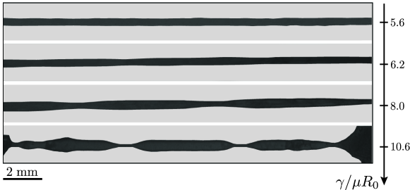
Figure 1: Equilibrium shape of agar gel cylinders for different values of the shear modulus. The radius is 240 $\mu$m, the surface tension is $\gamma$ = 37 mN/m. Adapted from Mora et al. (2010).

Our findings are important to recent developments in the mechanics of exceedingly soft elastic solids Andreotti et al. (2016); Style et al. (2017); Mora et al. (2010). As an example we quote the capillary instability of an elastic cylinder Entov and Yarin (1984); Mora et al. (2010); Eggers and Fontelos (2015); Xuan and Biggins (2017), as shown in Fig. 1. The cylinder consists of a fully cross-linked agar gel, and unlike viscoelastic liquids therefore exhibits a reference state that is free from elastic stress – one could call it an elastic solid rather than an elastic liquid. When sufficiently soft, however, the solid cylinder still exhibits a Rayleigh-Plateau instability that leads to the formation of thin threads. This resembles a bit the “bead-on-a-string” configuration, which is a well-known feature for thinning jets of dilute polymer suspensions Clasen et al. (2006). A natural question is whether the two systems can be described by the same continuum description.

The paper starts with a brief overview of the continuum formulations of elastic liquids and elastic solids in Section II. Particular emphasis is given to the kinematics of affine and non-affine motions in the limit $\lambda\rightarrow\infty$. Based on this, we propose in Section III an order parameter formulation for elastic liquids, which is similar in spirit to the work by Leonov Leonov (1976). We derive the energy equation and provide a systematic classification of polymer models – the most common models are summarized in Appendix A. At the end of the paper we present a numerical study of the capillary instability of elastic threads, highlighting the importance of the elastic limit (Section IV) and we close with a discussion (Section V).

II Classical continuum theory

II.1 Viscoelastic fluids

We consider an incompressible velocity field ${\bf v}({\bf x},t)$ (${\boldsymbol{\nabla}}\cdot{\bf v}=0$), described by the momentum balance

$$\rho\left(\frac{\partial{\bf v}}{\partial t}+{\bf v}\cdot{\boldsymbol{\nabla}}{\bf v}\right)={\boldsymbol{\nabla}}\cdot\boldsymbol{\sigma},$$ (1)

where $\boldsymbol{\sigma}$ is the stress tensor. The stress tensor is split into a Newtonian contribution (coming e.g. from a solvent) and a polymeric (viscoelastic) contribution $\boldsymbol{\sigma}_{p}$:

$$\boldsymbol{\sigma}=-p{\bf I}+\eta_{s}\dot{\boldsymbol{\gamma}}+\boldsymbol{\sigma}_{p}\equiv-p{\bf I}+\boldsymbol{\tau},$$ (2)

where the deviatoric stress $\boldsymbol{\tau}$ is the contribution excluding the pressure. Here we defined the rate-of-deformation tensor

$$\boldsymbol{\dot{\gamma}}=\left({\boldsymbol{\nabla}}{\bf v}\right)+\left({\boldsymbol{\nabla}}{\bf v}\right)^{T},$$ (3)

and $\eta_{s}$ is the solvent viscosity. Any isotropic contribution to the stress can be written as part of the pressure $p$.

The non-Newtonian contribution $\boldsymbol{\sigma}_{p}$ originates from the stretching of the microstructure inside the fluid. Though we will refer to $\boldsymbol{\sigma}_{p}$ as the “polymeric stress”, having in mind dilute polymer suspensions, the concept equally applies to emulsions whose microstructure is described by droplet deformations Mwasame et al. (2017, 2018). The non-Newtonian contribution $\boldsymbol{\sigma}_{p}$ is governed by a separate evolution equation, describing the state of the component governed by a long time scale $\lambda$, for example a polymer. We will see it is best to write the polymeric stress $\boldsymbol{\sigma}_{p}=\boldsymbol{\sigma}_{p}({\bf A})$ as a function of a state variable (or order parameter field) ${\bf A}$ that is a symmetric second rank tensor. This conformation tensor, which can be derived by coarse-graining microscopic models based on suspended beads-and-spring dumbbells Bird et al. (1987), has the property that the polymer stress vanishes when $\mathbf{A}=\mathbf{I}$, where $\mathbf{I}$ is the identity tensor. However, in this paper we follow a purely continuum approach, without referring to any microscopic model. In particular, we will give a precise continuum definition of the conformation tensor, and show that the structure of the dependence $\boldsymbol{\sigma}_{p}({\bf A})$ will be determined by the elastic limit $\lambda\rightarrow\infty$.

In the simplest case this relationship is linear,

$$\boldsymbol{\sigma}_{p}=\mu\left(\mathbf{A}-\mathbf{I}\right),$$ (4)

where $\mu$ has the dimensions of an elastic shear modulus. The state variable ${\bf A}$ must have the property that it evolves toward its relaxed state $\mathbf{A}=\mathbf{I}$ in the limit of long times. Once more, the simplest way of doing this to write a linear relaxation law

$$\dot{{\bf A}}=-\frac{1}{\lambda}\left({\bf A}-{\bf I}\right).$$

However, it is has been known for a long time Oldroyd (1950); Bird et al. (1987) that for the dynamics of a second-rank tensor to be frame invariant Morozov and Spagnolie (2015), i.e. to be independent of the frame of reference, the ordinary time derivative needs to be replaced by another derivative. There are two versions of this frame invariant derivative (and linear combinations thereof). The so-called upper convected derivative

$$\overset{\triangledown}{\bf A}=\frac{\partial{\bf A}}{\partial t}+{\bf v}\cdot{\boldsymbol{\nabla}}{\bf A}-\left({\boldsymbol{\nabla}}{\bf v}\right)^{T}\cdot{\bf A}-{\bf A}\cdot\left({\boldsymbol{\nabla}}{\bf v}\right),$$ (5)

is derived from the requirement that it transforms consistently as a covariant tensor. The first two terms on the right are the convected derivative of a material point, ensuring Galilean invariance, the last two terms make sure that ${\bf A}$ transforms correctly under deformations by the flow. We will see below that the upper convected derivative describes affine motion, that is a situation where each material point of the polymer follows the flow. This is seen most directly from beads-and-spring models of polymers Bird et al. (1987), from which the upper convected derivative follows automatically if beads are required to follow the flow without slip. However, a contravariant formulation would do equally well from the point of view of frame invariance, but yields a different derivative, known as the lower convected derivative:

$$\overset{\vartriangle}{\bf A}=\frac{\partial{\bf A}}{\partial t}+{\bf v}\cdot{\boldsymbol{\nabla}}{\bf A}+{\bf A}\cdot\left({\boldsymbol{\nabla}}{\bf v}\right)^{T}+\left({\boldsymbol{\nabla}}{\bf v}\right)\cdot{\bf A}.$$ (6)

Using the upper convected derivative, a linear relaxation law takes the form

$$\overset{\triangledown}{\mathbf{A}}=-\frac{1}{\lambda}\left(\mathbf{A}-\mathbf{I}\right),$$ (7)

which means that for any initial condition $\mathbf{A}$ relaxes exponentially toward $\mathbf{A}=\mathbf{I}$ on a time scale $\lambda$. Equations (4) and (7) can be combined into a single equation of motion for the polymeric stress:

$$\boldsymbol{\sigma}_{p}+\lambda\overset{\triangledown}{\boldsymbol{\sigma}}_{p}=\eta_{p}\boldsymbol{\dot{\gamma}},$$ (8)

which is a tensorial form of the simple Maxwell fluid; here $\eta_{p}=\mu\lambda$ is the polymeric viscosity. The stress tensor (2) together with (8) is known as the Oldroyd B model Bird et al. (1987); in the limit of vanishing rates of deformation, it describes a Newtonian fluid of total viscosity $\eta_{0}=\eta_{s}+\eta_{p}$.

Although the Oldroyd B model is very popular owing to its simplicity, there are many relevant physical effects which are not captured. For that reason there are many extensions of the Oldroyd B equations, for example taking into account non-linearity in both (4) and (7), or in the solvent contribution in (2). In Appendix A, we supply a list of various models. Apart from the question of frame invariance, models have to be consistent with requirements of thermodynamics Beris and Mavrantzas (1994); Mwasame et al. (2017, 2018); Beris and Edwards (1994); Öttinger (2005).

II.2 Elasticity

While fluid mechanics is usually formulated in an Eulerian frame, non-linear (finite deformation) elasticity is written in a Lagrangian formulation. This means that deformations are described by a mapping ${\bf x}={\bf x}({\bf X})$, where ${\bf x}$ is the position of a material point after the deformation, which used to be at ${\bf X}$ before the deformation. Elasticity is based on the idea that stresses in an isotropic medium can only depend on the change in distance between material points generated by a deformation Landau and Lifshitz (1984); Wik . Namely if ${\bf F}=\partial\mathbf{x}/\partial\mathbf{X}$ is the deformation gradient tensor, and $ds$ is the distance between two points which used to be a distance $dS$ apart, we obtain Landau and Lifshitz (1984); Wik , using $d{\bf x}={\bf F}\cdot d{\bf X}$, that

$$ds^{2}-dS^{2}=d\mathbf{X}^{T}\cdot\left(\mathbf{F}^{T}\cdot\mathbf{F}-{\bf I}\right)\cdot d\mathbf{X}.$$ (9)

Thus the energy of a deformation can only depend on Green’s deformation tensor ${\bf C}=\mathbf{F}^{T}\cdot\mathbf{F}$, which is a symmetric second rank tensor that is defined on the reference configuration (the tensor $({\bf F}^{T}\cdot{\bf F}-{\bf I})/2$ is called the finite strain tensor). The eigenvalues of $\mathbf{C}$ represent the principal stretches, i.e. the ratio of deformed over reference length along the principle directions of the deformation. Importantly, $\mathbf{C}$ shares the same eigenvalues as those of the Finger tensor Wik , defined as $\mathbf{B}=\mathbf{F}\cdot\mathbf{F}^{T}$. The Finger tensor is entirely defined on the current configuration, and is therefore more convenient when connecting to the Eulerian descriptions, as typically used for viscoelastic liquids. Since the elastic energy can only depend on invariants of ${\bf C}$, which are the same as those of ${\bf B}$, we can write $W=W({\bf B})$ for the elastic free energy density. Moreover, the function $W({\bf B})$ must have the property that it assumes a minimum for ${\bf B}={\bf I}$. This means that any deformation will cost energy, which is a necessary condition for the unstressed state to be stable.

Though not necessary, we from now on focus on incompressible media for which $\det\left({\mathbf{F}}\right)=1$. Once the free energy is specified, the (true) stress tensor for incompressible media follows as

$$\boldsymbol{\sigma}_{p}=\frac{\partial W}{\partial\mathbf{F}}\cdot\mathbf{F}^{T}=2\frac{\partial W}{\partial\mathbf{B}}\cdot\mathbf{B},$$ (10)

where in the second step we exploited the symmetry of $\mathbf{B}$. This expression is a consequence of the virtual work principle Truesdell and Noll (2004), requiring that any change of the elastic energy density satisfies

$$\frac{dW}{dt}=\boldsymbol{\sigma}_{p}:(\nabla\mathbf{v})^{T}=\frac{1}{2}\boldsymbol{\sigma}_{p}:\dot{\boldsymbol{\gamma}}$$ (11)

Landau and Lifshitz (1984), where in the second step we used the symmetry of $\boldsymbol{\sigma}_{p}$. The derivation of (10),(11) will be spelled out in the next section. As we argued before, $W$ can only be a function of one of the invariants of ${\bf B}$, which can be written as Wik

$$I_{1}=B_{kk},\quad\quad I_{2}=\frac{1}{2}\left(B_{kk}^{2}-B_{ij}B_{ij}\right),\quad\quad I_{3}=\det\mathbf{B},$$ (12)

where we remind that $I_{3}=\det({\bf F})^{2}=1$ for incompressible media. Hence, we can write the free energy as a function of the first two invariants only: $W(I_{1},I_{2})$. The constraint $I_{3}=1$ will be ensured by an isotropic pressure acting as a Lagrange multiplier.

Using (10), we obtain

$$\boldsymbol{\sigma}_{p}=2W_{1}\mathbf{B}+2W_{2}\left({\rm tr}(\mathbf{B})\mathbf{B}-\mathbf{B}\cdot\mathbf{B}\right),$$ (13)

where $W_{1}\equiv\partial W/\partial I_{1}$ and $W_{2}\equiv\partial W/\partial I_{2}$. This can be simplified using the Cayley-Hamilton theorem, which for $\det({\bf B})=1$ reads

$${\bf B}^{-1}={\bf B}^{2}-{\rm tr}({\bf B}){\bf B}+\frac{1}{2}\left({\rm tr}({\bf B})^{2}-{\rm tr}({\bf B}^{2})\right)\mathbf{I}.$$ (14)

As a result, the stress can be written as

$$\boldsymbol{\sigma}_{p}=2W_{1}\left(\mathbf{B}-\mathbf{I}\right)+2W_{2}\left(\mathbf{I}-\mathbf{B}^{-1}\right),$$ (15)

where for convenience we have absorbed an isotropic contribution into the pressure.

The derivatives $W_{1}$ and $W_{2}$ can be arbitrary non-linear functions of the invariants $I_{1}$ and $I_{2}$. If $W_{1}=\mu/2$ and $W_{2}=0$, one finds the neo-Hookean model, and using (15) one finds the stress to be $\boldsymbol{\sigma}_{p}=\mu\left(\mathbf{B}-\mathbf{I}\right)$, which corresponds to (4) with ${\bf A}\equiv{\bf B}$. The case where both $W_{1}$ and $W_{2}$ are constant but non-zero goes by the name of Mooney-Rivlin solid.

II.3 Kinematics: affine and non-affine motion

To make a connection between the Eulerian polymer models and the Lagrangian formulation of elasticity, we need to find out what are the deformations generated by transport by the velocity field ${\bf v}$. The velocity field is connected to the motion of material points by ${\bf v}=d\mathbf{x}/dt$, where $d/dt$ is a time derivative at constant material point $\mathbf{X}$. Then it follows from the chain rule that Morozov and Spagnolie (2015)

$$\frac{d{\bf F}}{dt}=\left({\boldsymbol{\nabla}}{\bf v}\right)^{T}\cdot{\bf F},\quad\frac{d{\bf F^{-1}}}{dt}=-{\bf F}^{-1}\cdot\left({\boldsymbol{\nabla}}{\bf v}\right)^{T},$$ (16)

where $\left({\boldsymbol{\nabla}}{\bf v}\right)_{ij}=\partial_{i}v_{j}$. The relation (16) permits to calculate the deformation gradient tensor from ${\bf v}$, and thus to pass from an Eulerian to a Lagrangian description. For later reference, we will derive a number of auxiliary kinematic relations. The first is obtained by taking the time derivative of the identity ${\bf x}\left({\bf X}({\bf x},t),t\right)={\bf x}$ at constant ${\bf x}$. Denoting the derivative at constant $\mathbf{x}$ by $\partial/\partial t$ and at constant ${\bf X}$ as $d/dt$, we have $0=d{\bf x}/dt+\partial\mathbf{x}/\partial\mathbf{X}\cdot\partial{\bf X}/\partial t$, and so the velocity ${\bf v}=d{\bf x}/dt$ can be calculated from

$${\bf v}=-{\bf F}\cdot\frac{\partial{\bf X}}{\partial t}.$$ (17)

Thus given the inverse Lagrangian map (or reference map Kamrin et al. (2012)) ${\bf X}({\bf x},t)$, the Eulerian velocity field can be retrieved. Note that (17) can also be written in the form

$$\frac{\partial{\bf X}}{\partial t}+{\bf v}\cdot{\boldsymbol{\nabla}}{\bf X}=0,$$ (18)

which expresses the fact that by definition the total derivative of the reference state ${\bf X}$ must vanish.

If the fluid is incompressible, the mapping ${\bf x}\left({\bf X},t\right)$ must be volume-preserving and so the Eulerian incompressibility condition ${\boldsymbol{\nabla}}\cdot{\bf v}=0$ is equivalent to $\det{\bf F}=1$. In the more general case of a compressible fluid, using the transformation formula for volumes, the Lagrangian condition simply changes to

$$\rho=\frac{\rho_{0}}{\det({\bf F})},$$ (19)

where $\rho_{0}$ is the density in reference coordinates. To confirm that in an Eulerian transformation, we take the convected time derivative of (19):

$$\frac{\partial\rho}{\partial t}+({\bf v}\cdot{\boldsymbol{\nabla}})\rho=\frac{d{\rho}}{dt}=\rho_{0}\frac{d{\det({\bf F}^{-1})}}{dt}=\rho_{0}{\rm tr}\left(\frac{\bf F}{\det({\bf F})}\frac{d{\bf F}^{-1}}{dt}\right)=-\frac{\rho_{0}}{\det({\bf F})}{\rm tr}\left({\boldsymbol{\nabla}}{\bf v}\right)=-\rho{\boldsymbol{\nabla}}\cdot{\bf v},$$

having used Jacobi’s formula Magnus and Neudecker (1999) in the third step, and (16) in the fourth. In other words, (19) is equivalent to

$$\frac{\partial\rho}{\partial t}+{\boldsymbol{\nabla}}\cdot(\rho{\bf v})=0,$$ (20)

the usual Eulerian form of the continuity equation.

Now we turn to the main point of interest, dealing with frame invariant time derivatives of an Eulerian tensor ${\bf A}(\mathbf{x},t)$, and relating it to the Lagrangian mapping. To achieve that, we derive the following identity relating the upper convective derivative and the time derivatives of the mapping:

$$\overset{\triangledown}{\bf A}={\bf F}\cdot\left[\frac{d}{dt}\left({\bf F}^{-1}\cdot{\bf A}\cdot{\bf F}^{-T}\right)\right]\cdot{\bf F}^{T}.$$ (21)

Indeed, making use of (16), the explicit evaluation of the time derivative gives (5).

The definition (21) has a natural interpretation. Since convection plays no role on the domain of material coordinates, one first projects the Eulerian tensor $\mathbf{A}$ back to the Lagrangian domain, using the inverse transformation ${\bf F}^{-1}\cdot{\bf A}\cdot{\bf F}^{-T}$. Then, once the time-derivative is performed on the Lagrangian domain, the result is returned to the Eulerian domain to yield an objective tensorial time-derivative. However, the above procedure is not unique. Namely, we can also construct a Lagrangian tensor as ${\bf F}^{T}\cdot{\bf A}\cdot{\bf F}$. This can be viewed as the transformation of a covariant tensor (while ${\bf F}^{-1}\cdot{\bf A}\cdot{\bf F}^{-T}$ gives the transformation of a contravariant tensor) Morozov and Spagnolie (2015). Following the same procedure as above, this gives an alternative time derivative

$$\overset{\vartriangle}{\bf A}={\bf F}^{-T}\cdot\left[\frac{d}{dt}\left({\bf F}^{T}\cdot{\bf A}\cdot{\bf F}\right)\right]\cdot{\bf F}^{-1},$$ (22)

where the lower convective derivative is defined in (6).

II.3.1 Affine motion

This produces the sought-after connection between polymer dynamics and elasticity: in the limit $\lambda\rightarrow\infty$ the derivative vanishes, so the upper convected models reduce to $\overset{\triangledown}{\bf A}=0$. Thus multiplying (21) by ${\bf F}^{-1}$ from the left and ${\bf F}^{-T}$ from the right, and integrating over time, we find

$${\bf F}^{-1}\cdot{\bf A}\cdot{\bf F}^{-T}={\rm constant}\quad\Rightarrow\quad{\bf A}={\bf F}\cdot\mathbf{D}_{0}\cdot{\bf F}^{T},$$ (23)

where $\mathbf{D}_{0}$ is a constant (time-independent) Lagrangian tensor that is independent of the mapping; $\mathbf{D}_{0}$ can be viewed as an integration constant and can be determined from initial conditions. A natural choice is to consider the initial condition ($\mathbf{F}=\mathbf{I}$) to be stress-free, i.e. $\boldsymbol{\sigma}_{p}=0$ which implies $\mathbf{A}=\mathbf{I}$. Hence, we find $\mathbf{D}_{0}=\mathbf{I}$, i.e. $\mathbf{A}={\bf B}\equiv\mathbf{F}\cdot\mathbf{F}^{T}$.

In other words, given a relaxation law of the form $\lambda\overset{\triangledown}{\bf A}=f({\bf A})$, in the limit $\lambda\rightarrow\infty$ the upper convected derivative implies that ${\bf A}$ tracks the stretching induced by the flow, as described by (9): the deformation follows the flow affinely. The conformation tensor $\mathbf{A}$ in viscoelasticity plays the same role as the Finger tensor $\mathbf{B}$ in elasticity. If on the other hand the relaxation law would imply $\overset{\vartriangle}{\bf A}=0$, using (22) we find $\mathbf{A}={\bf B}^{-1}\equiv\mathbf{F}^{-T}\cdot\mathbf{F}^{-1}$, which would correspond to an elastic response in a direction opposite the flow. Let us illustrate these two cases using the simple elongational flow

$$v_{r}=-\dot{\epsilon}r,\quad v_{z}=2\dot{\epsilon}z.$$ (24)

Integrating (16) with initial condition ${\bf F}={\bf I}$ one obtains

$$\mathbf{B}=\begin{pmatrix}e^{-2\dot{\epsilon}t}&0\\ 0&e^{4\dot{\epsilon}t}&\end{pmatrix},\quad{\mathbf{B}}^{-1}=\begin{pmatrix}e^{2\dot{\epsilon}t}&0\\ 0&e^{-4\dot{\epsilon}t}&\end{pmatrix}.$$ (25)

In other words, ${\bf B}$ describes stretching in the $z$-direction and contraction in the radial direction that is generated by the flow $\mathbf{v}$, while ${\bf B}^{-1}$ does the exact opposite.

II.3.2 Non-affine motion

By combining the upper and lower derivatives, one can describe a situation where the polymer deformation partially follows the flow, making it non-affine to a certain degree. To show this, we consider the derivative introduced in the Johnson-Segalman model Johnson Jr. and Segalman (1977) which takes into account the possibility that the polymer does not follow the flow of the solvent in an affine fashion, but slips with respect to the flow. This is accomplished by introducing the polymer velocity $\mathbf{v}_{a}$, which satisfies

$${\boldsymbol{\nabla}}{\bf v}_{a}=\frac{a}{2}\left[{\boldsymbol{\nabla}}{\bf v}+({\boldsymbol{\nabla}}{\bf v})^{T}\right]+\frac{1}{2}\left[{\boldsymbol{\nabla}}{\bf v}-({\boldsymbol{\nabla}}{\bf v})^{T}\right]=\frac{1+a}{2}{\boldsymbol{\nabla}}{\bf v}-\frac{1-a}{2}({\boldsymbol{\nabla}}{\bf v})^{T},$$ (26)

where $a$ (the so-called slip parameter) satisfies $-1\leq a\leq 1$. Indeed, for $a=1$, ${\boldsymbol{\nabla}}{\bf v}_{a}$ and ${\boldsymbol{\nabla}}{\bf v}$ are the same, and the polymer follows perfectly. This is no longer the case for $a\neq 1$. The antisymmetric part of ${\boldsymbol{\nabla}}{\bf v}_{a}$ and ${\boldsymbol{\nabla}}{\bf v}$ are the same, which means ${\bf v}_{a}$ and ${\bf v}$ have the same vorticity, so that the polymer follows any solid body rotation of the flow perfectly. On the other hand, the rate of deformation of the polymer (symmetric part) satisfies $\dot{\boldsymbol{\gamma}}_{a}=a\dot{\boldsymbol{\gamma}}$. The Johnson-Segalman derivative is the upper convected derivative with respect to the slipping polymer:

$$\overset{\triangledown}{\left(\bf A\right)}_{a} \equiv \frac{d{\mathbf{A}}}{dt}-\left({\boldsymbol{\nabla}}{\bf v}_{a}\right)^{T}\cdot{\mathbf{A}}-{\mathbf{A}}\cdot\left({\boldsymbol{\nabla}}{\bf v}_{a}\right)=\frac{1+a}{2}\overset{\triangledown}{\mathbf{A}}+\frac{1-a}{2}\overset{\vartriangle}{\mathbf{A}}.$$ (27)

Here we remind that in the following $d/dt$ denotes the material derivative.

To illustrate the consequences of the non-affine motion, we consider a relaxation law based on the Johnson-Segalman derivative. In that case, one obtains $\overset{\triangledown}{\left(\bf A\right)}_{a}=0$ in the limit of large relaxation times. We solve this equation for a uniform shear flow $\mathbf{v}=\dot{\gamma}y\mathbf{e}_{x}$, and take the initial conditions as $\mathbf{A}=\mathbf{I}$. Solving for ${\bf A}$, one obtains the oscillatory response:

$${\bf A}=\begin{pmatrix}\frac{1}{(1-a)}\left[1-a\cos\left(\sqrt{1-a^{2}}\dot{\gamma}t\right)\right]&\frac{a}{\sqrt{1-a^{2}}}\sin\left(\sqrt{1-a^{2}}\dot{\gamma}t\right)\\ \frac{a}{\sqrt{1-a^{2}}}\sin\left(\sqrt{1-a^{2}}\dot{\gamma}t\right)&\frac{1}{(1+a)}\left[1+a\cos\left(\sqrt{1-a^{2}}\dot{\gamma}t\right)\right]\end{pmatrix}.$$ (28)

Clearly, this does not correspond to any elastic model. Physically, the oscillations can be understood from the non-affine kinematics dictated by (26). The flow $\mathbf{v}=\dot{\gamma}y\mathbf{e}_{x}$ can be written as a superposition of an elongational flow and a rigid body rotation, which are exactly equal of amplitude. Any slip ($a<1$) removes part of the elongation flow, while the full rigid body rotation is retained. This effectively leads to an “excess” rigid body motion, that gives rise to a periodic “flow” of the polymer, with a frequency $\sqrt{1-a^{2}}\dot{\gamma}$. We remark that these oscillations have a purely kinematic origin, and thus persist for a Johnson-Segalman fluid that is sheared at finite values of $\lambda$. In that case, however, the oscillations are damped so that $\mathbf{A}$, and hence the polymer stress, eventually reaches a steady state Larson (1999).

From these observations we draw an important conclusion. When the order parameter $\mathbf{A}$ tracks the stretching of the polymer, just like the Finger tensor $\mathbf{B}$ does in the theory of elasticity, the relaxation law must be constructed from the upper convected derivative. Only then, one can make sure that the polymer deformation is purely elastic in the limit $\lambda\rightarrow\infty$, in the sense that it follows the deformation imposed by the flow. Any other time-derivative implies non-affine motion. The very same conclusions were reached in the context of emulsions, whose drops deform into ellipsoids – in that case the eigenvalues of $\mathbf{A}$ represent the square of the semi-axes of the deformed droplets Mwasame et al. (2017, 2018).

III Order parameter formulation of rheological models

Using arguments similar to those of Leonov (1976), now we want to combine the above observations, in order to formulate a class of models which separate the description of viscoelastic stress into two different aspects; as shown in more detail in Appendix B, the eigenvalues of the conformation tensor $\mathbf{A}$ represent the stretching of the polymer. The first aspect concerns the energetics of the problem, from which one can calculate the stress. The second aspect describes the relaxation of ${\bf A}$, from which we calculate the dissipation. Taken together, this provides us with a systematic procedure to find the equation describing the total energy. To summarize, we have the following ingredients:

1. A symmetric rank-2 tensor order parameter field $\mathbf{A}(\mathbf{x},t)$, which quantifies the stretched state of the polymer.

2. An elastic free energy density $W(\mathbf{A})$, which is minimal for $\mathbf{A}=\mathbf{I}$.

3. A relaxation equation towards $\mathbf{A}=\mathbf{I}$, governing dissipation.

The physical structure we are trying to embody in $\mathbf{A}$, using these requirements, has been characterized as an “instantaneous reference state” in Tanner (2000). At each instant, if the flow were to stop, the instantaneous reference state tends to the current state. In terms of the curvilinear formalism (cf. Appendix B), the conformation tensor relates to the difference between the “instantaneous reference metric”, and the actual “current metric”. The former relaxes to the latter.

To find the correct structure of $W(\mathbf{A})$, we borrow from the elastic energy $W(\mathbf{B})$, as found on non-linear elasticity. The energy must be a function of the invariants

$$I_{1}=A_{kk},\quad\quad I_{2}=\frac{1}{2}\left(A_{kk}^{2}-A_{ij}A_{ij}\right),\quad\quad I_{3}=\det\mathbf{A},$$ (29)

with ${\bf A}$ taking the role of ${\bf B}$ in (12). There should be no confusion from using the same notation for the invariants of ${\bf A}$. The choice of $W(\mathbf{A})$ naturally determines the elastic limit, while the relaxation equation for $\mathbf{A}$ accounts for irreversible dissipation.

We now proceed to derive the expression for the stress and the dissipation, focusing first on affine polymer models, for which the conformation tensor relaxes according to $\lambda\overset{\triangledown}{\bf A}=f({\bf A})$. The idea is that the reversible part of the deformation has the same form as the reversible change in free energy (11), so the remainder corresponds to dissipation. Writing the work in symmetric form $\frac{1}{2}\boldsymbol{\sigma}_{p}:\dot{\boldsymbol{\gamma}}$, and introducing the volumetric dissipation rate $\epsilon_{p}$, we find

$$\frac{1}{2}\boldsymbol{\sigma}_{p}:\dot{\boldsymbol{\gamma}}=\frac{dW}{dt}+\epsilon_{p}.$$ (30)

This expresses that any work done during the deformation must either be stored in elastic energy, or be dissipated. With this convention, $\epsilon_{p}$ must be positive in order to be consistent with thermodynamics. The time derivative $dW/dt$ can be calculated using the definition of $\overset{\triangledown}{\bf A}$, yielding

$$\frac{dW}{dt} = \frac{\partial W}{\partial\mathbf{A}}:\frac{d\mathbf{A}}{dt}=\frac{\partial W}{\partial\mathbf{A}}:\left[\left({\boldsymbol{\nabla}}{\bf v}\right)^{T}\cdot\mathbf{A}+\mathbf{A}\cdot\left({\boldsymbol{\nabla}}{\bf v}\right)+\overset{\triangledown}{\bf A}\right]$$ (31)

$$= \left(\frac{\partial W}{\partial\mathbf{A}}\cdot\mathbf{A}\right):\dot{\boldsymbol{\gamma}}+\frac{\partial W}{\partial\mathbf{A}}:\overset{\triangledown}{\bf A},$$

where in the last line we made use of the symmetry $\mathbf{A}$. As anticipated in (30), this nicely separates into a term due to deformation $\dot{\boldsymbol{\gamma}}$ and to a term associated to the relaxation law. Equating $dW/dt$ in (31) and (30), we obtain the expression for stress.

$$\boldsymbol{\sigma}_{p}=2\frac{\partial W}{\partial\mathbf{A}}\cdot\mathbf{A}.$$ (32)

As expected, this is exactly the form of the elastic stress (10), with ${\bf A}$ replacing ${\bf B}$. The remainder can be identified as the dissipation

$$\epsilon_{p}=-\frac{\partial W}{\partial\mathbf{A}}:\overset{\triangledown}{\bf A}.$$ (33)

We are now in a position to formulate the energy balance for a polymeric liquid. Multiplying (1) by ${\bf v}$, using (2), we obtain

$$\frac{1}{2}\frac{\partial\rho v^{2}}{\partial t}+{\boldsymbol{\nabla}}\cdot\left[\left(\frac{\rho v^{2}}{2}+p\right){\bf v}-\eta_{s}\dot{\boldsymbol{\gamma}}\cdot{\bf v}-\boldsymbol{\sigma}_{p}\cdot{\bf v}\right]=-\epsilon-\frac{1}{2}\boldsymbol{\sigma}_{p}:\dot{\boldsymbol{\gamma}},$$ (34)

where

$$\epsilon=\frac{\eta_{s}}{2}\dot{\boldsymbol{\gamma}}:\dot{\boldsymbol{\gamma}}$$ (35)

is the viscous dissipation. Using $\boldsymbol{\sigma}_{p}:\dot{\boldsymbol{\gamma}}/2=dW/dt+\epsilon_{p}$ this can be rewritten as

$$\frac{d}{dt}\left(\frac{\rho v^{2}}{2}+W\right)+{\boldsymbol{\nabla}}\cdot\left[p{\bf v}-\eta_{s}\dot{\boldsymbol{\gamma}}\cdot{\bf v}-\boldsymbol{\sigma}_{p}\cdot{\bf v}\right]=-\epsilon-\epsilon_{p},$$ (36)

which has the form of a conservation law for the sum of kinetic energy $\rho v^{2}/2$ and elastic energy $W$. The term in square brackets is the energy flux. The right hand side represents the dissipation, which has a viscous contribution from the solvent $\epsilon$, and a polymeric contribution $\epsilon_{p}$, which according to (33) is associated with the relaxation of ${\bf A}$. The conservation law (36), together with the expressions for the stress (32) and the dissipation (33), are the main results of this paper.

In the remainder we restrict ourselves to incompressible order parameters for which $\det(\mathbf{A})=1$ (this restriction could be lifted if necessary), which makes $W$ a function of $I_{1},I_{2}$ only: $W(I_{1},I_{2})$. Evaluating the elastic stress (32) is a essentially a repeat of the elastic calculation (10),(15), and $\boldsymbol{\sigma}_{p}$ has the same form:

$$\boldsymbol{\sigma}_{p}=2W_{1}\left(\mathbf{A}-\mathbf{I}\right)+2W_{2}\left(\mathbf{I}-\mathbf{A}^{-1}\right),$$ (37)

but is based on the conformation tensor $\mathbf{A}$ rather than on the Finger tensor $\mathbf{B}$. The relaxation of the conformation tensor gives rise to dissipation $\epsilon_{p}$, which using $W(I_{1},I_{2})$ and (33) becomes

$$\epsilon_{p}=-\left[W_{1}\mathbf{I}+W_{2}{\rm tr}(\mathbf{A})\mathbf{I}-W_{2}\mathbf{A}\right]:\overset{\triangledown}{{\mathbf{A}}}.$$ (38)

It is evident that dissipation vanishes in the absence of relaxation $\overset{\triangledown}{{\mathbf{A}}}=0$; in this case $\mathbf{A}=\mathbf{B}$, so that we recover the full structure of elasticity theory.

As an aside, we note that (38) can be written in a more elegant form, using the lower convected derivative. Namely, using the identity

$${\rm tr}({\bf A}){\rm tr}(\overset{\triangledown}{\bf A})-{\bf A}:\overset{\triangledown}{\bf A}={\rm tr}(\overset{\vartriangle}{\left(\mathbf{A}^{-1}\right)}),$$

we can also write $\epsilon_{p}$ in the form

$$\epsilon_{p}=-W_{1}{\rm tr}(\overset{\triangledown}{\bf A})-W_{2}{\rm tr}\overset{\vartriangle}{\left(\mathbf{A}^{-1}\right)},$$ (39)

so that the full energy balance takes the form

$$\frac{d}{dt}\left(\frac{\rho v^{2}}{2}+W\right)-{\boldsymbol{\nabla}}\cdot\left[\boldsymbol{\sigma}\cdot{\bf v}\right]=-\epsilon-W_{1}tr(\overset{\triangledown}{\bf A})-W_{2}tr\overset{\vartriangle}{\left(\mathbf{A}^{-1}\right)}.$$ (40)

III.1 Examples

Let us discuss a number of viscoelastic models that are captured by the present approach. A more detailed list is found in Appendix A. As regards the validity of a certain model, the subtle question concerns the relaxation equation for ${\bf A}$, which here we take of the form $\lambda\overset{\triangledown}{\bf A}=f({\bf A})$, so that deformations follows the flow affinely. Non-affine motion will be considered below. In addition, it has to be checked that the model is consistent with thermodynamics and that in particular, $\epsilon_{p}>0$.

First, we consider the Oldroyd B model, where relaxation equation is known as the upper convected Maxwell model. The model is defined by a neo-Hookean elastic energy, while the relaxation is linear, i.e.

$$W=\frac{\mu}{2}\left(I_{1}-3\right),\quad\overset{\triangledown}{{\mathbf{A}}}=-\frac{1}{\lambda}\left(\mathbf{A}-\mathbf{I}\right).$$ (41)

Hence, the stress (37) and dissipation (38) follow as Hohenegger and Shelley (2011):

$$\boldsymbol{\sigma}_{p}=\mu\left(\mathbf{A}-\mathbf{I}\right),\quad\epsilon_{p}=\frac{\mu(I_{1}-3)}{2\lambda}=\frac{W}{\lambda}.$$ (42)

Note that since $W$ must be positive (it acquires its minimum for ${\bf A}={\bf I}$ where it is zero), this implies that $\epsilon_{p}\geq 0$, as required.

Second, in both the energy and the relaxation equation, there can appear nonlinear functions of the invariants. The most popular of such models is the FENE-P model Bird et al. (1987); Larson (1999). Like other models of the same kind, it is based on the concept of an elastic spring attached to two beads in solution. While a Hookean, non-interacting spring leads to the Oldroyd B equation, here the spring is non-linear, so that it cannot be extended beyond a limiting length $L$. This avoids the deficiency of the Oldroyd B model, that the polymeric stress grows exponentially to infinity in a strong flow. In the non-linear case the model can no longer be solved exactly, so various approximations are used of which FENE-P is one. The finite extensibility is introduced so that $I_{1}\equiv{\rm tr}(\mathbf{A})$ reaches a maximum value $L^{2}$, via the stress relation

$$\boldsymbol{\sigma}_{p}=\mu F(I_{1})\left(\mathbf{A}-\mathbf{I}\right),\quad\mathrm{with}\quad F(I_{1})=\frac{L^{2}-3}{L^{2}-I_{1}}.$$ (43)

Clearly, the stress diverges when $I_{1}=L^{2}$. This stress relation is complemented by a nonlinear relaxation law

$$\overset{\triangledown}{\mathbf{A}}=-\frac{1}{\lambda}\left(F(I_{1})\mathbf{A}-\mathbf{I}\right),$$ (44)

which reduces to $\overset{\triangledown}{\mathbf{A}}=0$ for infinite relaxation time. It is now an easy task to identify the rubber model that emerges in the elastic limit. Namely, from (37) we can find the elastic energy as

$$W=\frac{\mu}{2}(L^{2}-3)\ln\left(F(I_{1})\right),$$ (45)

which in rubber elasticity is known as the Gent model. Using that in the elastic limit $\mathbf{A}=\mathbf{F}\cdot\mathbf{F}^{T}$ and $I_{1}={\rm tr}(\mathbf{F}\cdot\mathbf{F}^{T})$, the corresponding stress reads

$$\boldsymbol{\sigma}_{p}=\mu F(I_{1})\left(\mathbf{F}\cdot\mathbf{F}^{T}-\mathbf{I}\right).$$ (46)

This shows how the viscoelastic FENE-P model is naturally connected to the Gent model. We remark that the FENE-CR model Chilcott and Rallison (1988) has the same energetic structure as the FENE-P model, but with a slightly different relaxation law, namely $\overset{\triangledown}{\mathbf{A}}=-F(I_{1})\left(\mathbf{A}-\mathbf{I}\right)/\lambda$.

More generally, models that only involve the first invariant $I_{1}$ must have a relaxation equation of the form

$$\overset{\triangledown}{\mathbf{A}}=-\frac{1}{\lambda}\left(g_{1}(I_{1})\mathbf{A}-g_{0}(I_{1})\mathbf{I}\right),$$ (47)

since any multiples of the type $\mathbf{A}\cdot\mathbf{A}$ would, upon taking the trace, produce a second invariant $I_{2}$. Hence, the dissipation for $I_{1}$-based models becomes

$$\epsilon_{p}=\frac{W_{1}}{\lambda}\left[I_{1}g_{1}(I_{1})-3g_{0}(I_{1})\right].$$ (48)

Given that $W_{1}>0$, thermodynamic consistency $\epsilon\geq 0$ is then ensured by

$$I_{1}g_{1}(I_{1})-3g_{0}(I_{1})\geq 0\quad\mathrm{for}\quad I_{1}\geq 3.$$ (49)

The FENE-P and FENE-CR models indeed fall within this class.

III.2 Non-affine models

So far we have dealt with the physical situation that the constituents follow the flow exactly. As discussed in Subsection II.3, using a derivative which is a linear superposition of upper and lower convected derivatives, one can model a situation where the material “slips” relative to the flow. In that case, dissipative processes are described by the relaxation equation in the slipping frame, leading to a form $\lambda\overset{\triangledown}{\left(\bf A\right)}_{a}=f({\bf A})$, where $\overset{\triangledown}{\left(\bf A\right)}_{a}$ is defined in (27), which is the upper convected derivative in the polymer frame.

In order to split $dW/dt$ into a part that depends on the deformation and a part that depends on the relaxation, we use $\overset{\triangledown}{\left(\bf A\right)}_{a}$ instead of $\overset{\triangledown}{\bf A}$ to obtain

$$\frac{dW}{dt}=\frac{\partial W}{\partial\mathbf{A}}:\frac{d\mathbf{A}}{dt}=\left(a\frac{\partial W}{\partial\mathbf{A}}\cdot\mathbf{A}\right):\dot{\boldsymbol{\gamma}}+\frac{\partial W}{\partial\mathbf{A}}:\overset{\triangledown}{\left(\bf A\right)}_{a}.$$ (50)

We therefore find the stress and dissipation, respectively, as

$$\boldsymbol{\sigma}_{p}=2a\frac{\partial W}{\partial\mathbf{A}}\cdot\mathbf{A},\quad\quad\epsilon_{p}=-\frac{\partial W}{\partial\mathbf{A}}:\overset{\triangledown}{\left(\bf A\right)}_{a},$$ (51)

where $\boldsymbol{\sigma}_{p}$ has the same form as (10), but with a factor $a$ in front of the expression for the stress. This reflects the slip: the polymer is stretched less than expected, making the response “softer” by a fraction $a$. By consequence, the stress can be further expressed as

$$\boldsymbol{\sigma}_{p}=2aW_{1}\left(\mathbf{A}-\mathbf{I}\right)+2aW_{2}\left(\mathbf{I}-\mathbf{A}^{-1}\right).$$ (52)

A Johnson-Segalman fluid is characterized by a simple neo-Hookean energy, $W_{1}=\mu/2$ and $W_{2}=0$, complemented by a linear relaxation equation in the slipping frame

$$\overset{\triangledown}{\left(\bf A\right)}_{a}=\frac{1+a}{2}\overset{\triangledown}{\bf A}+\frac{1-a}{2}\overset{\vartriangle}{\bf A}=-\frac{1}{\lambda}\left(\mathbf{A}-\mathbf{I}\right).$$ (53)

Hence instead of (42) we have

$$\boldsymbol{\sigma}_{p}=a\mu\left(\mathbf{A}-\mathbf{I}\right),\quad\epsilon_{p}=\frac{\mu(I_{1}-3)}{2\lambda}=\frac{W}{\lambda}.$$ (54)

In particular, it follows that the dissipation is always positive, and vanishes in the limit $\lambda\rightarrow\infty$. Indeed, one verifies that (53) with $\lambda=\infty$ is invariant under the symmetry $t\mapsto-t$, $\mathbf{v}\mapsto-\mathbf{v}$. So upon reversing the flow, the system dynamics retraces its path and there is no relaxation of $\mathbf{A}$ in the frame co-moving with the polymer. Remarkably, however, we have seen that owing to non-affine motion, there is an oscillatory response to a shear deformation. By consequence, even though the “elastic limit” is non-dissipative and invariant upon time reversal, it does not correspond to any elastic solid. Perhaps this is related to the fact that within the formalism developed by Beris and Edwards Beris and Edwards (1994), the Johnson-Segalman model has a contribution from the dissipation bracket, even at infinite relaxation time, indicating aspects of irreversible behavior.

As a particular example we consider the case of perfect counterflow, $a=-1$, with a neo-Hookean energy for the polymer, $W=\frac{1}{2}\mu(I_{1}-3)$. According to the above, we recover the lower convected Maxwell model

$$\boldsymbol{\sigma}_{p}=-\mu\left(\mathbf{A}-\mathbf{I}\right),\quad\overset{\vartriangle}{\bf A}=-\frac{1}{\lambda}\left(\mathbf{A}-\mathbf{I}\right),$$ (55)

which can be written as

$$\boldsymbol{\sigma}_{p}+\lambda\overset{\vartriangle}{\boldsymbol{\sigma}}_{p}=\eta_{p}\boldsymbol{\dot{\gamma}},$$ (56)

as opposed to (8) for the upper convected version. We previously concluded that the in corresponding elastic limit, since $\overset{\vartriangle}{\bf A}=0$, we had $\mathbf{A}=\mathbf{B}^{-1}$. This gives the elastic stress

$$\boldsymbol{\sigma}_{p}=\mu\left({\bf I}-{\bf B}^{-1}\right).$$

Comparing to (15), we find that this corresponds to a rubber model with an energy $W=\frac{1}{2}\mu(I_{2}^{\bf B}-3)$, based on the second invariant of the Finger tensor, $I^{\mathbf{B}}_{2}$. This is consistent with a neo-Hookean energy for $\mathbf{A}$, since using the Cayley-Hamilton theorem (14) one verifies that $I^{\mathbf{B}}_{2}=I^{\mathbf{B}^{-1}}_{1}=I^{\mathbf{A}}_{1}$ for incompressible media.

In general, we thus conclude that any non-affine motion $a\neq 1$ does not converge to an elastic-solid response in the limit of large relaxation time. Formally, on the level of stress, the special case of perfect counterflow does converge to a special type of elastic solid that is based on the second invariant of $\mathbf{B}$. However, no realistic rubber is described only by the second invariant of the deformation (Truesdell and Noll, 2004, p. 158), Mihai and Goriely (2017). This can be rationalized by the fact that the polymer needs to deform oppositely to the imposed flow.

IV Collapse of a cylinder under surface tension

Figure 2: High-speed video-image of a jet (radius 0.3 mm) of dilute (0.01 wt%) aqueous polyacrylamide solution undergoing capillary thinning Clasen et al. (2006). The relaxation time of the polymer is $\lambda=0.012$ s.

We now illustrate our observations by considering a more complex example including a free surface: the breakup of a liquid column under the action of surface tension Clasen et al. (2006); Eggers and Fontelos (2015); Turkoz et al. (2018). This is illustrated in Fig. 2, showing the breakup of a water jet containing a low concentration of a high molecular flexible polymer, with a relaxation time of about 0.01 seconds. The breakup process repeats itself periodically, so one can see an almost cylindrical thread at different stages of thinning. An alternative geometry is that of a liquid bridge between two plates, which leads to a single thread. In each case, the thread radius is observed to thin exponentially Bazilevskii et al. (1997); Clasen et al. (2006); Turkoz et al. (2018), with a rate of decay $1/(3\lambda)$ in the case of a single timescale.

Using a lubrication description, it was conjectured by Entov and Yarin Entov and Yarin (1984) and confirmed in Clasen et al. (2006); Turkoz et al. (2018) that the shape of the thinning thread could be described, at least for sufficiently slow polymer relaxation, by a fluid with infinite relaxation time. In that case, since stresses do not relax, one expects the liquid to converge toward a stationary state, where surface tension and elastic forces are balanced Entov and Yarin (1984); Mora et al. (2010); Eggers and Fontelos (2015). Our work shows that, for example in the framework of an Oldroyd B fluid, the limit $\lambda\rightarrow\infty$ corresponds exactly to minimizing the sum of elastic and surface tension energy for a neo-Hookean material. This has previously been shown only in the lubrication limit Entov and Yarin (1984); Eggers and Fontelos (2015). Within a lubrication description, it can be shown that a stationary state will still be reached for a Johnson-Segalman fluid, as long as the slip coefficient $a>1/2$. However, below we will show that this result appears to be an artefact of the lubrication (or slender-jet) approximation. Our full simulations show that no stationary state is reached as soon as $a$ falls short of the affine limit $a=1$.

To test these ideas, we simulate the Oldroyd B equations (1),(2) in the limit of $\lambda\rightarrow\infty$, taken such that $\mu=\eta/\lambda$ remains finite. Then the polymeric stress is governed by $\overset{\triangledown}{\boldsymbol{\sigma}}_{p}=0$. The collapse is driven by surface tension, and the stress boundary condition at the free surface is

$${\bf n}\cdot\boldsymbol{\sigma}=-\kappa{\bf n},$$ (57)

where

$$\kappa=\frac{1}{h(1+h_{z}^{2})^{1/2}}-\frac{h_{zz}}{(1+h_{z}^{2})^{\frac{3}{2}}},\quad{\bf n}=\frac{{\bf e}_{r}-{\bf e}_{z}h_{z}}{(1+h_{z}^{2})^{1/2}}$$ (58)

are (twice) the mean curvature and the surface normal, respectively. If $h(z,t)$ is the thread profile, the kinematic boundary condition becomes

$$\frac{\partial h}{\partial t}+u_{z}(z,h)\frac{\partial h}{\partial z}=u_{r}(z,h),$$ (59)

where ${\bf v}=u_{r}{\bf e}_{r}+u_{z}{\bf e}_{z}$ in cylindrical coordinates. As an initial condition, we take the free surface shape

$$h(z,0)\equiv h_{0}(z)=R_{0}\left[1-\epsilon\cos\left(\frac{z}{2R_{0}}\right)\right],$$ (60)

and both the velocity field and stresses vanish initially. Boundary conditions are periodic.

We have carried out a simulation for a fluid cylinder of radius $R_{0}$, which is slightly perturbed according to (60) with $\epsilon=0.05$, $\eta_{s}/\sqrt{\rho\gamma R_{0}^{3}}=0.79$ and $\mu R_{0}/\gamma=0.0119$. In order to calculate the nonlinear time evolution of the flow, we apply the boundary fitted coordinate method, where the liquid domain is mapped onto a rectangular domain through a coordinate transformation. The hydrodynamic equations are discretized in this domain using fourth-order finite differences, with 22 equally spaced points in the radial direction and 1000 equally spaced points in the axial direction. An implicit time advancement is performed using second-order backward finite differences with a fixed time step $0.05\sqrt{\rho R_{0}^{3}/\gamma}$; details of the numerical procedure can be found elsewhere Herrada and Montanero (2016).

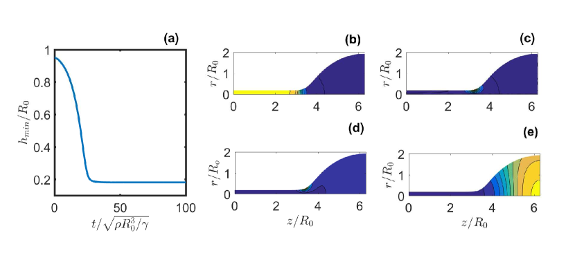
Figure 3: (a) Time evolution of the minimum thread radius for the viscoelastic fluid simulation with $\epsilon=0.05$, $\eta_{s}/\sqrt{\rho\gamma R_{0}^{3}}=0.79$ and $\mu R_{0}/\gamma=0.0119$. Polymeric stresses in the final state of the fluid simulation: (b) $\sigma_{p,zz}$; (c) $\sigma_{p,zr}$; (d) $\sigma_{p,rr}$; (e) $\sigma_{p,\theta\theta}.$ The purple to yellow color gradient grows from minimum to maximum stress.

In Fig. 3-(a) we show the minimum thread radius, $h_{min}$, as function of time. As the bridge collapses, elastic stress builds up until it is balanced by surface tension, as seen in Fig. 3. At this point the solution becomes stationary, time derivatives vanish, and the velocity goes to zero. As a result, the solvent viscosity does not affect the final state, seen in Fig. 3-(b)-(d), which shows the different components of the stress tensor. The axial stress $\sigma_{p,zz}$ is highest inside the thread, where fluid elements are stretched the most in the axial direction. Radial stresses $\sigma_{p,rr}$, on the other hand, are most pronounced inside the drop, where fluid elements are stretched in the radial direction.

IV.1 The neo-Hookean solid

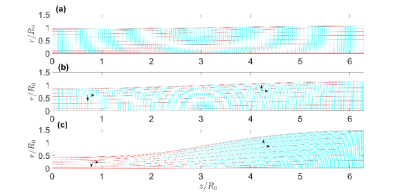
Figure 4: The elastic simulation: (a) The reference state, $\mu R_{0}/\gamma=\infty$; (b) $\mu R_{0}/\gamma=0.2$; (c) $\mu R_{0}/\gamma=0.1.$ Red (cyan) lines describe constant values of $\eta$ ($\xi$). The arrows indicate the direction of the mesh deformation.

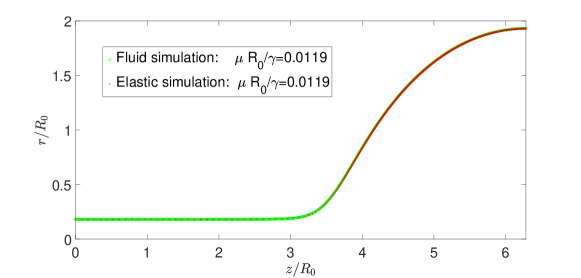
Figure 5: A comparison between the final shape of an elastic bridge driven by surface tension, using an Oldroyd B fluid with $\lambda=\infty$ (green) and a neo-Hookean elastic material (red). The results are identical.

We now calculate the steady state of an elastic neo-Hookean material using non-linear elasticity, as described by

$$\boldsymbol{\sigma}=\mu\left(\mathbf{F}\cdot\mathbf{F}^{T}-\mathbf{I}\right)-p{\bf I}$$ (61)

and subject to the incompressibility constraint $J=\det(\mathbf{F})=1$. The pressure is adjusted such that $J=1$ is satisfied. Instead of a dynamical equation, the condition for equilibrium reads $\nabla\cdot\boldsymbol{\sigma}=\mathbf{0}$, i.e. (1) with $\mathbf{v}=\mathbf{0}$, with elasto-capillary boundary condition (57).

To determine the final state of the collapsed cylinder, we have to solve a nonlinear set of equations corresponding to the above conditions, based on a mapping ${\bf x}={\bf x}({\bf X})$. To this end, we write the mapping in cylindrical coordinates: $r=r(R,Z)$, $z=z(R,Z)$. The coordinates $R$ and $Z$ are the radial and axial coordinates of the cylinder in the reference state. Using general formulae for ${\bf F}$ in cylindrical coordinates Negahban (2012) , incompressibility amounts to

$$\det{\bf F}=\frac{r}{R}\left(\frac{\partial r}{\partial R}\frac{\partial z}{\partial Z}-\frac{\partial r}{\partial Z}\frac{\partial z}{\partial R}\right)=1,$$ (62)

while the stress can be computed from the finger tensor

$$\mathbf{B}=\mathbf{F}\cdot\mathbf{F}^{T}=\begin{pmatrix}\left(\left(\frac{\partial r}{\partial R}\right)^{2}+\left(\frac{\partial r}{\partial Z}\right)^{2}\right)&0&\left(\frac{\partial r}{\partial R}\frac{\partial z}{\partial R}+\frac{\partial r}{\partial Z}\frac{\partial z}{\partial Z}\right)\\ 0&\left(\frac{r}{R}\right)^{2}&0\\ \left(\frac{\partial r}{\partial R}\frac{\partial z}{\partial R}+\frac{\partial r}{\partial Z}\frac{\partial z}{\partial Z}\right)&0&\left(\left(\frac{\partial z}{\partial Z}\right)^{2}+\left(\frac{\partial z}{\partial R}\right)^{2}\right)\end{pmatrix}.$$ (63)

The solution depends on the dimensionless number $R_{0}\mu/\gamma$. In the “soft” limit where the thread becomes very thin $r\ll R_{0}$, the thickness is of thread scales as the elasto-capillary length scale Eggers and Fontelos (2015)

$$\ell_{e}=\left(\frac{\mu R_{0}^{4}}{\gamma}\right)^{1/3}.$$ (64)

To solve the problem numerically, we define the reference state by

$$R=h_{0}(\xi)\eta,\quad Z=\xi,$$

with the elastic domain defined by $\eta\in[0,1]$ and $\xi\in[0,2\pi R_{0}]$; $h_{0}$ is once again defined by (60), and $\epsilon=0.05.$ We are looking for two unknown functions $f$ and $g$, where $r=r(R,Z)=f(\eta,\xi)$ and $z=z(R,Z)=g(\eta,\xi)$, as well as the pressure $p(\eta,\xi)$. These three unknowns are found from solving the three equations (62), (1) at steady state, and (57). The free surface $h(z)$ then is given by the parametric representation $h(g(1,\xi))=f_{1}(1,\xi)$, from which the curvature $\kappa$ can be evaluated. The domain is discretized using fourth-order finite differences with 301 equally spaced points in the $\xi$ direction and 11 Chebyshev collocation points in the $\eta$ direction. For the results presented in Fig. 5, a finer mesh was used with 2001 equally spaced points in the $\xi$ direction.

The resulting system of non linear equations is solved using a Newton-Raphson technique Herrada and Montanero (2016). We solve the problem by starting with the reference state as initial guess and $\mu R_{0}/\gamma$ sufficiently large ($\mu R_{0}/\gamma=100$) to ensure the convergence of the Newton-Raphson iterations. Once we get a solution, we use this solution in a new run with a smaller value of $\mu R_{0}/\gamma$.

The result is shown in Fig. 4, which describes the deformation of the mesh as well as of the free surface, for various values of $\mu R_{0}/\gamma$. The resulting shapes closely resemble those in Fig. 1 at moderate stiffness, and agree with simulations in Xuan and Biggins (2017). In Fig. 5 we compare the elastic equilibrium state (red dots) with the stationary state reached in the simulation of the Oldroyd-B model for $\mu R_{0}/\gamma=0.0119$. The agreement is perfect – illustrating that Oldroyd-B converges to neo-Hookean in the limit of $\lambda\rightarrow\infty$, as we have shown in the present paper. A detailed similarity analysis of this problem is provided in Eggers et al. (2019).

IV.2 The Johnson-Segalman fluid

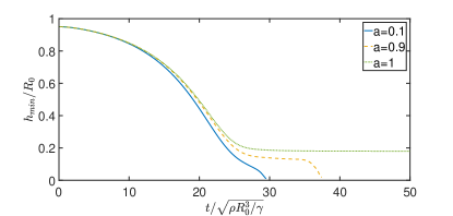
Figure 6: The minimum thread radius $h_{min}$ for a Johnson-Segalman fluid, as a function of time for for different values of $a$. Only in the case of non-affine motion ($a=1$), the thread attains a static elastic solution. Breakup is observed for all values $a\neq 1$.

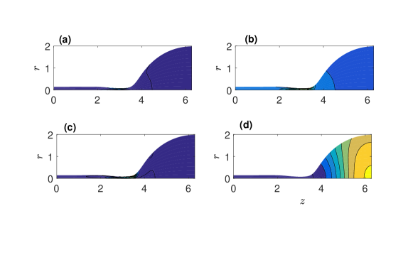
Figure 7: Polymeric stresses at a time close to the breakup of the Johnson-Segalman fluid simulation with $a=0.9$: (a) $\sigma_{p,zz}$; (b) $\sigma_{p,zr}$; (c) $\sigma_{p,rr}$; (d) $\sigma_{p,\theta\theta}$. The purple to yellow colour gradient grows from minimum to maximum stress.

The above comparison was an illustration of our result which assigns a unique elastic limit to the Oldroyd B model for large relaxation times. Now we consider a Johnson-Segalman fluid with infinite relaxation time, characterized by $\overset{\triangledown}{\left(\mathbf{A}\right)}_{a}=0$. The other equations remain the same. Previous analysis of the long-wavelength limit has shown Eggers and Fontelos (2015) that there can be no surface tension - elastic balance for $a<1/2$. This result was obtained through an analysis of a thread of uniform thickness. However, since the true solution is not a uniform thread throughout, $a>1/2$ is only a necessary condition for a stationary state.

Johnson-Segalman fluid simulations are carried out by integrating (53) with $\lambda=\infty$ for different values of $a$ with the same numerical technique described at the beginning of the section, using the same parameters $\epsilon=0.05$, $\eta_{s}/\sqrt{\rho\gamma R_{0}^{3}}=0.79$, and $\mu R_{0}/\gamma=0.0119$ as before. Figure 6 shows $h_{min}$ as function of time for three different values of the slip parameter $a$. As it can be seen in the figure, the solution reaches a steady state only for the affine case $a=1$ while for the other cases the numerical solution breaks. Particular interesting is the case, $a=0.9$, which according to the lubrication analysis should reach a stationary state. However, as seen in Fig. 7, the solution is qualitatively different from the case $a=1$: the thread becomes non-uniform in space and continues to evolve in time until the solution breaks.

IV.3 A mixed Eulerian-Lagrangian method for neo-Hookean solid and Newtonian fluids

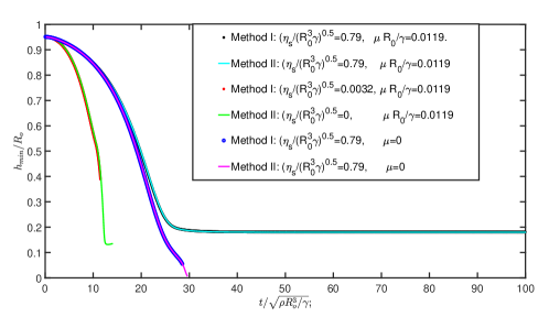
Figure 8: A comparison of the Eulerian method based on the Oldroyd-B equations (method I), and the mixed Eulerian-Lagrangian method based on finding the Lagrangean map (method II) for the collapse of a liquid bridge. The time evolution of the minimum thread radius is shown for three different materials: (i) an elastic liquid with solvent (black, cyan), (ii) a purely elastic liquid without solvent (red, green), and (iii) a Newtonian liquid (blue, magenta).

In the above, we have compared numerical simulations to investigate the elastic limit $\lambda\rightarrow\infty$. On one hand, we have employed purely Eulerian ideas using the Oldroyd-B equations, as shown in Fig. 3, to advance the state of the system in time. Eventually, a steady state is reached, and since the velocity goes to zero, the solvent does not contribute to the stress, and the steady state represents a purely elastic balance. However, taking $\eta_{s}$ to zero represents a very singular limit, since the velocity disappears from the momentum equation (1), apart from inertial terms on the left, which are very small.

On the other hand, we used the purely Lagrangian description (61), where the Finger tensor ${\bf B}$ is given in terms of the Lagrangian map ${\bf x}({\bf X},t)$. By solving the nonlinear equation ${\boldsymbol{\nabla}}\cdot\boldsymbol{\sigma}=\mathbf{0}$, we can find the equilibrium state, which is in perfect agreement with the long-time limit of the Eulerian simulation, as seen in Fig. 5.

By using the transformations between Eulerian and Lagrangian formulations layed out in Section II.3, we can construct a much more versatile method, which combines the advantages of both. Instead of Eulerian fields, everything is solved for the mapping ${\bf x}({\bf X},t)$. Calculating derivatives, we obtain the deformation gradient tensor ${\bf F}$, as well as $\partial{\bf X}/\partial t$, from which we find the Eulerian velocity ${\bf v}$ via (17). Instead of the incompressibility condition ${\boldsymbol{\nabla}}\cdot{\bf v}=0$, we implement $J=\det({\bf F})=1$. if we were to deal with a compressible liquid, we could use (19) instead of the continuity equation.

To illustrate that we are able to go all the way from an elastic solid to a pure viscous liquid using the same method, we consider the total stress (2) in the limit $\lambda\rightarrow\infty$, so that we can write

$$\boldsymbol{\sigma}=\mu\left(\mathbf{F}\cdot\mathbf{F}^{T}-\mathbf{I}\right)+\eta_{s}\boldsymbol{\dot{\gamma}}-p{\bf I}.$$ (65)

For $\mu>0$ and $\eta_{s}=0$, (65) corresponds to a neo-Hookean solid, while if $\mu=0$ and $\eta_{s}>0$ the material is a pure Newtonian fluid.

In order to solve the problem numerically, we need to be able to compute partial derivatives of in both the current state and in the reference state. To achieve that, a numerical reference domain $\eta\in[0,1]$ and $\xi\in[0,2\pi R_{0}]$ is introduced. The current and reference state are both mapped to the numerical domain through

$$R=R_{n}(\xi,\eta,t),\quad Z=Z_{n}(\xi,\eta,t);\quad r=r_{n}(\xi,\eta,t)\quad z=z_{n}(\xi,\eta,t)$$

at each point in time. To close the system of equations for these additional unknowns, we have chosen to set

$$R_{n}=h_{0}(Z_{n})\eta,\quad z_{n}=\xi,$$ (66)

where $h_{0}$ is once again defined by (60), and $\epsilon=0.05.$ This choice allows us to keep a steady distribution of points in the axial direction in the current state.

In summary, we are looking for the unknown functions $r_{n}(\xi,\eta,t)$ ,$z_{n}(\xi,\eta,t)$, $R_{n}(\xi,\eta,t)$, $Z_{n}(\xi,\eta,t)$ $v_{z}(\xi,\eta,t)$, $v_{r}(\xi,\eta,t)$, and $p(\xi,\eta,t)$. These seven unknowns are found from solving the momentum equation (1) with stress (65), the incompressibility constraint (62), the velocity (17), the mapping (66), and the free surface condition (57). Then the free surface $h(z,t)$ is given by the parametric representation $h(z_{n}(\xi,\eta,t),t)=r_{n}(\xi,1,t)$, from which the curvature $\kappa$ can be evaluated. For the simulations reported in Fig. 8, the domain is discretized using fourth-order finite differences with 801 equally spaced points in the $\xi$ direction and 11 Chebyshev collocation points in the $\eta$ direction. An implicit time step is performed using second-order backward finite differences with a fixed time step $0.01\sqrt{\rho R_{0}^{3}/\gamma}$. The resulting system of nonlinear equations is solved using a Newton-Raphson technique Herrada and Montanero (2016).

In Fig. 8 we show the minimum thread radius, $h_{\rm min}$, as function of time for three different materials using the mixed Eulerian-Lagrangian approach (method II, solid lines). These results are compared to our earlier Eulerian approach, using the Oldroyd-B equations (method I, symbols). The results are virtually identical, but the method II is often found to be more stable, in particular at small values of the solvent viscosity, since the Eulerian method becomes singular in that limit.

The black dots (method I) and solid cyan line (method II) corresponds to the case considered in the previous section, for which $\eta_{s}>0$, and for which the system evolves toward a steady state. This is seen in Fig. 8 by the fact that $h_{\rm min}$ approaches and then stays at a constant value, representing a elastic capillary balance. The black dots (method I) are the same data as seen before in Fig. 3, but the cyan line now shows the complete time evolution toward the steady state, using the Lagrangian map; the two results are indistinguishable from one another.

The red dots (method I) are for the same system, but with a very small solvent viscosity. However, the method fails even before coming close to a stationary state, owing to the singular nature of the small-$\eta_{s}$ limit. The solid green line (method II) corresponds to a pure neo-Hookean solid, and can now been treated owing to the mixed Euler-Lagrangian method. The initial dynamics represent a balance between elasticity and inertia, and is much more rapid since in this case there is not dissipation ($\eta_{s}=0$). Up to the point where the Eulerian method fails, there is close agreement between both methods. As elastic stress builds up, the inertial motion is arrested suddenly, and the bridge rebounds. This deforms the interface so much that the mapping (66)) becomes singular, and the numerics break down, because the shape can no longer be represented properly.

Finally, putting $\mu=0$ and letting $\eta_{s}$ remain finite, we obtain a pure Newtonian fluid, in which there are no more elastic stresses. Both methods (blue dots, method I, solid magenta curve, method II), deliver the same result, in which there are no elastic stresses to balance surface tension. As a result, the solution pinches off in finite time, with the minimum radius $h_{\rm min}$ a linear function of time Eggers and Villermaux (2008). In our numerical examples we have only considered cases with infinite relaxation time, but the Eulerian-Lagrangian scheme would work equally well for a finite $\lambda$, which interpolates smoothly between fluid and elastic behavior.

V Discussion

In summary, we have provided a detailed overview of how viscoelastic models are related to the theory of elasticity. By analyzing the kinematics in the limit of large relaxation times, we have identified a systematic route to express the energy balance in viscoelastic flows. This is based on the separation of the reversible elastic energy from the dissipation associated to relaxation phenomena. Our observations are illustrated by a detailed analysis of the capillary instability of a cylindrical jet, analyzed for both elastic and viscoelastic materials. An important observation is that the presence of non-affine motion in polymer solutions has a dramatic effect, as it will lead to pinching of the thread even in the limit of infinite relaxation times. This illustrates that non-affine viscoelastic liquids do not have any counterpart within the theory of elasticity.

From a general viewpoint, the explicit connection between elasticity and viscoelasticity may provide an original perspective to problems in either fields. For example, in Eggers et al. (2019) we have exploited the elastic correspondence to resolve the breakup of viscoelastic threads, which are traditionally studied e.g. by Oldroyd-B or FENE-P models. From a numerical perspective, the analysis developed here provides a new approach towards computational challenges. For example, the neo-Hookean simulation for elastic threads turned out to be very efficient, and we have demonstrated how such schemes can also be extended to Newtonian fluids. Conversely, we note that using viscoelastic liquids with infinite relaxation time could offer an attractive, fully Eulerian approach to fluid-structure interaction problems.

Appendix A Rheological models

Here we list a number of frequently considered rheological models, and show how they fit into our formalism, which consists in specifying an elastic energy $W({\bf A})$ as well as a relaxation equation $\lambda\overset{\triangledown}{\bf A}=f({\bf A},\dot{\boldsymbol{\gamma}})$. Then the polymeric stress as well as the dissipation can be calculated from (32) and (33) in the affine case, and (42) for the non-affine case.

1. Oldroyd B / Upper convected Maxwell model
   

   As described in Subsection III.1, in that case the equations can be written

   $$\boldsymbol{\sigma}_{p}=\mu\left(\mathbf{A}-\mathbf{I}\right),\quad\overset{\triangledown}{{\mathbf{A}}}=-\frac{1}{\lambda}\left(\mathbf{A}-\mathbf{I}\right);$$ (67)

   the elastic energy and dissipation are

   $$W=\frac{\mu}{2}\left({\rm tr}({\bf A})-3\right),\quad\epsilon_{p}=\frac{W}{\lambda}.$$ (68)

   According to (2), the deviatoric stress $\boldsymbol{\tau}$ is the sum of solvent and polymer contributions. In the Oldroyd B model, both can be combined into the single equation

   $$\boldsymbol{\tau}+\lambda\overset{\triangledown}{{\boldsymbol{\tau}}}=\eta\dot{\boldsymbol{\gamma}}+\lambda\eta_{s}\overset{\triangledown}{\dot{\boldsymbol{\gamma}}}.$$ (69)

   In the limit of vanishing shear rate, (69) describes a Newtonian fluid of total viscosity $\eta=\eta_{s}+\eta_{p}$, the sum of polymeric and solvent contributions.

2. Oldroyd A / Lower convected Maxwell model
   

   As described in Subsection III.2,

   $$\boldsymbol{\sigma}_{p}=-\mu\left(\mathbf{A}-\mathbf{I}\right),\quad\overset{\vartriangle}{\bf A}=-\frac{1}{\lambda}\left(\mathbf{A}-\mathbf{I}\right),$$ (70)

   describes the evolution, and

   $$W=\frac{\mu}{2}\left({\rm tr}({\bf A})-3\right),\quad\epsilon_{p}=\frac{W}{\lambda}.$$ (71)

   are elastic energy and dissipation, respectively.

3. FENE-P model
   

   As discussed in Subsection III.1, with $I_{1}={\rm tr}(\mathbf{A})$ and $f(I_{1})=\frac{L^{2}-3}{L^{2}-I_{1}}$,

   $$\boldsymbol{\sigma}_{p}=\mu f(I_{1})\left(\mathbf{A}-\mathbf{I}\right),\quad\overset{\triangledown}{{\mathbf{A}}}=-\frac{1}{\lambda}\left(f(I_{1})\mathbf{A}-\mathbf{I}\right).$$ (72)

   so that

   $$W=\frac{\mu}{2}(L^{2}-3)\ln\left(f(I_{1})\right),\quad\epsilon_{p}=\frac{\mu}{2\lambda}f(I_{1})\left(I_{1}f(I_{1})-3\right),$$ (73)

   using (39).

4. Giesekus model
   

   This is a phenomenological model Bird et al. (1987); Larson (1999) which introduces a term quadratic in $\sigma_{p}$ into the equation of motion, which also limits the maximum value of the stress; however, the stress may become arbitrarily large for sufficiently strong flow:

   $$\boldsymbol{\sigma}_{p}+\lambda\overset{\triangledown}{\boldsymbol{\sigma}}_{p}+\alpha\frac{\lambda}{\eta_{p}}{\boldsymbol{\sigma}}_{p}\cdot{\boldsymbol{\sigma}}_{p}=\eta_{p}\boldsymbol{\dot{\gamma}}.$$ (74)

   This can be written as

   $$\boldsymbol{\sigma}_{p}=\mu\left(\mathbf{A}-\mathbf{I}\right),\quad\overset{\triangledown}{{\mathbf{A}}}=-\frac{1}{\lambda}\left[{\bf A}-{\bf I}+\alpha\left({\bf A}-{\bf I}\right)^{2}\right],$$ (75)

   so that the elastic energy is once more neo-Hookean, and the dissipation is:

   $$W=\frac{\mu}{2}\left(I_{1}-3\right),\quad\epsilon_{p}=\frac{\mu}{2\lambda}\left(I_{1}-3\right)+\frac{\mu\alpha}{2\lambda}\left({\bf A}:{\bf A}-2{\rm tr}({\bf A})+3\right).$$ (76)

5. Johnson-Segalman model
   

   As laid out in Subsection III.2, the Johnson-Segalman model is written

   $$\boldsymbol{\sigma}_{p}=a\mu\left(\mathbf{A}-\mathbf{I}\right),\quad(\overset{\triangledown}{{\mathbf{A}}})_{a}=-\frac{1}{\lambda}\left(\mathbf{A}-\mathbf{I}\right).$$ (77)

   The energy is once more neo-Hookean, and the dissipation is according to (51):

   $$W=\frac{\mu}{2}\left(I_{1}-3\right),\quad\epsilon_{p}=\frac{\mu}{2\lambda}\left(I_{1}-3\right)=\frac{W}{\lambda}.$$ (78)

Appendix B Curvilinear formulation of viscoelasticity

B.1 Kinematics of deformation

The purpose of this appendix is to rephrase the results of the main text in terms of curvilinear coordinates. This allows for a rigorous analysis of the physical assumptions underlying the equation of motion for the conformation tensor, $\mathbf{A}$. For a detailed description of kinematics discussed below, the reader can refer to the book by Green & Zerna Green and Zerna (2002).

We thus define curvilinear coordinates $q^{i}$, which are material points that move along affinely with the flow. The current position vector is defined as $\mathbf{x}(q^{i},t)$, while the position of the reference (or initial) configuration reads $\mathbf{X}(q^{i})=\mathbf{x}(q^{i},t=0)$. The latter is independent of time. The distance $ds$ between two neighboring points $q^{i}$ and $q^{i}+dq^{i}$ reads

$$ds^{2}=\left(\frac{\partial\mathbf{x}}{\partial q^{i}}\cdot\frac{\partial\mathbf{x}}{\partial q^{j}}\right)dq^{i}dq^{j}=g_{ij}dq^{i}dq^{j},$$ (79)

where $g_{ij}$ is the current metric tensor. Similarly, the reference distance $dS$ follows as

$$dS^{2}=\left(\frac{\partial\mathbf{X}}{\partial q^{i}}\cdot\frac{\partial\mathbf{X}}{\partial q^{j}}\right)dq^{i}dq^{j}=G_{ij}dq^{i}dq^{j},$$ (80)

where $G_{ij}$ is the reference metric. Stretching of material elements follows from changes in length

$$ds^{2}-dS^{2}=\left(g_{ij}-G_{ij}\right)dq^{i}dq^{j},$$ (81)

so strain is encoded in the difference between current and reference metric.

We now construct the current vector space, using the covariant and contravariant basis vectors

$$\mathbf{e}_{i}=\frac{\partial\mathbf{x}}{\partial q^{i}},\quad\mathbf{e}^{j}=\frac{\partial q^{j}}{\partial\mathbf{x}},$$ (82)

derived from the current position $\mathbf{x}$. The covariant basis vectors $\mathbf{e}_{i}$ are local tangents to the material lines in the deformed configuration. The contravariant vectors $\mathbf{e}^{i}$ form a reciprocal basis, owing to the property $\mathbf{e}_{i}\cdot\mathbf{e}^{j}=dq^{j}/dq^{i}=\delta_{i}^{j}$. Using this basis, we can define the metrics

$$g_{ij}=\mathbf{e}_{i}\cdot\mathbf{e}_{j},\quad g^{ij}=\mathbf{e}^{i}\cdot\mathbf{e}^{j},$$ (83)

so that $g_{ij}$ can be used to lower indices, while the inverse $g^{ij}$ raises indices. Similarly, one can construct the reference vector space, using “reference” basis vectors

$$\mathbf{E}_{i}=\frac{\partial\mathbf{X}}{\partial q^{i}},\quad\mathbf{E}^{j}=\frac{\partial q^{j}}{\partial\mathbf{X}}.$$ (84)

The associated metric for this basis, as well as its inverse, are defined by

$$G_{ij}=\mathbf{E}_{i}\cdot\mathbf{E}_{j},\quad G^{ij}=\mathbf{E}^{i}\cdot\mathbf{E}^{j};$$ (85)

the $\mathbf{E}_{i}$ are local tangents to the material lines in the reference configuration.

We now wish to express the metrics in terms of the mapping $\mathbf{F}=\partial\mathbf{x}/\partial\mathbf{X}$. In particular, we wish to show that Green’s deformation tensor $\mathbf{C}=\mathbf{F}^{T}\cdot\mathbf{F}$ and the Finger tensor $\mathbf{B}=\mathbf{F}\cdot\mathbf{F}^{T}$ can be written as

$$\mathbf{C}=g_{ij}\mathbf{E}^{i}\otimes\mathbf{E}^{j},\quad\mathbf{B}=G^{ij}\mathbf{e}_{i}\otimes\mathbf{e}_{j}.$$ (86)

To demonstrate this, we write (79) as

$$ds^{2}=\left(\frac{\partial\mathbf{x}}{\partial\mathbf{X}}\cdot\frac{\partial\mathbf{X}}{\partial q^{i}}\right)^{T}\cdot\left(\frac{\partial\mathbf{x}}{\partial\mathbf{X}}\cdot\frac{\partial\mathbf{X}}{\partial q^{j}}\right)dq^{i}dq^{j}=\mathbf{E}_{i}\cdot\left(\mathbf{F}^{T}\cdot\mathbf{F}\right)\cdot\mathbf{E}_{j}\,dq^{i}dq^{j}.$$ (87)

Comparing to (79), we indeed see that $g_{ij}$ are the covariant components of $\mathbf{C}=\mathbf{F}^{T}\cdot\mathbf{F}$ when expressed using the basis $\mathbf{E}^{i}$. Hence, we obtain the first identity in (86). It is important to keep track of the basis used to express the tensor Hanna (2019); for example, pairing $g_{ij}$ with the basis $\mathbf{e}^{i}$, one recovers the identity tensor, $\mathbf{I}=g_{ij}\mathbf{e}^{i}\otimes\mathbf{e}^{j}$.

Similarly we rewrite (80) as

$$dS^{2}=\left(\frac{\partial\mathbf{X}}{\partial\mathbf{x}}\cdot\frac{\partial\mathbf{x}}{\partial q^{i}}\right)^{T}\cdot\left(\frac{\partial\mathbf{X}}{\partial\mathbf{x}}\cdot\frac{\partial\mathbf{x}}{\partial q^{j}}\right)dq^{i}dq^{j}=\mathbf{e}_{i}\cdot\left(\mathbf{F}^{-T}\cdot\mathbf{F}^{-1}\right)\cdot\mathbf{e}_{j}\,dq^{i}dq^{j}.$$ (88)

Now we see that $G_{ij}$ are the covariant components of $\mathbf{B}^{-1}=\mathbf{F}^{-T}\cdot\mathbf{F}^{-1}$ when expressed using the basis $\mathbf{e}^{i}$. Since the inverse of the reference metric is defined as $G_{ik}G^{kj}=\delta^{j}_{i}$, we obtain the second identity in (86). Again, pairing $G_{ij}$ with the basis $\mathbf{E}^{i}$, one recovers the identity tensor, $\mathbf{I}=G_{ij}\mathbf{E}^{i}\otimes\mathbf{E}^{j}$.

B.2 Flow

Now, we investigate the effect of flow on the metric. First, we define the velocity as

$$\mathbf{v}=\left(\frac{d\mathbf{x}}{dt}\right)_{q^{i}}=v^{i}\mathbf{e}_{i},$$ (89)

expressed using the basis defined by (82), where from now on $d/dt$ means time-derivative at constant material points $q^{i}$. Using (83) and (82), the time-derivative of the metric tensor is

$$\frac{dg_{ij}}{dt} = \left(\frac{\partial\left(v^{k}\mathbf{e}_{k}\right)}{\partial q^{i}}\cdot\mathbf{e}_{j}\right)+\left(\mathbf{e}_{i}\cdot\frac{\partial\left(v^{m}\mathbf{e}_{m}\right)}{\partial q^{j}}\right)\equiv\left(v^{k}_{;i}\mathbf{e}_{k}\right)\cdot\mathbf{e}_{j}+\mathbf{e}_{i}\cdot\left(\mathbf{e}_{m}\right)v^{m}_{;j}$$ (90)

$$= g_{kj}v^{k}_{;j}+g_{mi}v^{m}_{;j}=v_{j;i}+v_{i;j}\equiv\dot{\gamma}_{ij},$$

where we used the definition of the covariant derivative, denoted by $(..)_{;j}$. Hence, the rate of strain tensor $\dot{\boldsymbol{\gamma}}$ directly gives the change of the metric of material coordinates by the flow. Remembering that $B^{ij}=G^{ij}$ (cf. (86)), we see that the Finger tensor evolves according to

$$\frac{dB^{ij}}{dt}=\frac{d}{dt}\left(\frac{\partial q^{i}}{\partial\mathbf{X}}\cdot\frac{\partial q^{j}}{\partial\mathbf{X}}\right)=0$$ (91)

during flow. This time-derivative vanishes because the reference state $\mathbf{X}(q^{i})$ is independent of time. Note, however, that the covariant components $B_{ij}$ are not constant in time, since

$$\frac{dB_{ij}}{dt}=\frac{d}{dt}\left(g_{ik}g_{jm}B^{km}\right)=2\dot{\gamma}_{ik}B^{k}_{j}.$$ (92)

For a general tensor $\mathbf{A}$, the derivatives $dA^{ij}/dt$ and $dA_{ij}/dt$ respectively correspond to the components of the upper and lower convected derivatives Oldroyd (1950); Aris (1990), i.e.

$$\overset{\triangledown}{{\mathbf{A}}}=\frac{dA^{ij}}{dt}\mathbf{e}_{i}\otimes\mathbf{e}_{j},\quad\quad\overset{\vartriangle}{{\mathbf{A}}}=\frac{dA_{ij}}{dt}\mathbf{e}^{i}\otimes\mathbf{e}^{j}.$$ (93)

The equivalence with the definitions (21) and (22) follow from transforming $A^{ij}$ respectively $A_{ij}$ from the Lagrangian (co-moving) material coordinates $q^{i}$, to an Eulerian coordinate system $\bar{q}^{i}$ that is fixed in space. In this fixed coordinate system, the tensor components indicated $\bar{A}^{ij}$ can be obtained using the transformation $F^{k}_{i}=\partial\bar{q}^{k}/\partial q^{i}$. Transforming $dA^{ij}/dt$ to the fixed frame then gives

$$F^{p}_{i}\left(\frac{dA^{ij}}{dt}\right)F^{q}_{j} = F^{p}_{i}\frac{d}{dt}\left[(F^{-1})^{i}_{k}\bar{A}^{km}(F^{-1})^{j}_{m}\right]F^{q}_{j}.$$ (94)

On the right hand side we recognize the definition (21) for $\overset{\triangledown}{{\mathbf{A}}}$, now in the form of the components of the fixed Eulerian system $\bar{q}^{i}$. In similar fashion one derives (93) for the lower convected derivative. Hence, $dB^{ij}/dt=0$ implies that the upper convected derivative of the Finger tensor vanishes, i.e. $\overset{\triangledown}{{\mathbf{B}}}=0$.

B.3 Elasticity

In the theory of elasticity, the energy density $W$ is a function of the invariants of $\mathbf{B}$. Assuming incompressibility $I_{3}=\det(\mathbf{B})=1$, the energy is of the form $W(I_{1},I_{2})$, where the first and second invariants are defined as

$$I_{1}=B^{i}_{i}=g_{ij}B^{ij},\quad I_{2}=\frac{1}{2}\left(\left[g_{ij}B^{ij}\right]^{2}-B_{ij}B^{ij}\right)=\frac{1}{2}\left(\left[g_{ij}B^{ij}\right]^{2}-g_{im}g_{jn}B^{mn}B^{ij}\right).$$ (95)

The expression for stress is obtained from time-derivatives, according to the virtual work principle,

$$\frac{1}{2}\sigma^{ij}\dot{\gamma}_{ij}=\frac{dW}{dt}=W_{1}\frac{dI_{1}}{dt}+W_{2}\frac{dI_{2}}{dt}.$$ (96)

Using $dB^{ij}/dt=0$, we find

$$\frac{dI_{1}}{dt}=\frac{dg_{ij}}{dt}B^{ij}=\dot{\gamma}_{ij}B^{ij},\quad\frac{dI_{2}}{dt}=\frac{dg_{ij}}{dt}\frac{\partial I_{2}}{\partial g_{ij}}=\dot{\gamma}_{ij}\left(I_{1}B^{ij}-B^{i}_{n}B^{nj}\right),$$ (97)

both of which are proportional to $\dot{\gamma}_{ij}$. Hence, from (96) we can read off the stress as

$$\sigma^{ij}=2\frac{\partial W}{\partial g_{ij}}=2W_{1}B^{ij}+2W_{2}\left(I_{1}B^{ij}-B^{i}_{n}B^{nj}\right).$$ (98)

B.4 Viscoelasticity

When an elastic liquid is suddenly arrested, the polymer will relax towards an isotropic equilibrium confirmation. The system slowly forgets about the history of deformation prior to the arrest, and all stress and polymer stretches are ultimately relaxed. When expressing the polymer deformation in terms of the elementary lengths between $q^{i}$ and $q^{i}+dq^{i}$, we can still write

$$ds^{2}-dS^{2}=\left(g_{ij}-G_{ij}\right)dq^{i}dq^{j},$$ (99)

and we associate an elastic energy to the polymer strain. Owing to the fading memory of the initial state $\mathbf{x}(q^{i},t=0)$, however, the object $G_{ij}$ can no longer be identified with the time-independent metric of this initial condition. Instead, $G_{ij}$ reflects the metric of the “instantaneous reference state” $\mathbf{X}(q^{i},t)$ that progressively tends to evolve towards the current state. Hence, using (85) and (84), we obtain

$$G_{ij}=\frac{\partial\mathbf{X}}{\partial q^{i}}\cdot\frac{\partial\mathbf{X}}{\partial q^{i}},\quad G^{ij}=\frac{\partial q^{i}}{\partial\mathbf{X}}\cdot\frac{\partial q^{j}}{\partial\mathbf{X}}.$$ (100)

We now wish to define the conformation tensor $\mathbf{A}$ whose eigenvalues give the stretches of the polymer. This is in direct analogy to Finger tensor $\mathbf{B}$, the only difference being that the stretches need to be measured with respect to the instantaneous reference state $\mathbf{X}(q^{i},t)$, rather than $\mathbf{x}(q^{i},t=0)$. Hence, we can define

$$\mathbf{A}=\left(\frac{\partial q^{i}}{\partial\mathbf{X}}\cdot\frac{\partial q^{j}}{\partial\mathbf{X}}\right)\mathbf{e}_{i}\otimes\mathbf{e}_{j},$$ (101)

where now the components $A^{ij}$ are time-dependent due to the relaxation of $\mathbf{X}(q^{i},t)$. If we wish to express this relaxation directly in terms of the conformation tensor $\mathbf{A}$, we arrive at

$$\frac{dA^{ij}}{dt}=\frac{1}{\lambda}f^{ij}(\mathbf{A}),$$ (102)

where the right hand side is independent of the flow, since any time dependence only enters through the reference state $\mathbf{X}(q^{i},t)$. By contrast, the covariant components $A_{ij}=g_{ik}g_{jm}A^{km}$ exhibit a time-dependence due to the flow $dg_{ij}/dt$ and due to the relaxation of $\mathbf{X}(q^{i},t)$. Hence, to quantify the relaxation in terms of the conformation tensor $\mathbf{A}$, one automatically singles out the upper convected derivatives as the appropriate time derivative.

In analogy with elasticity theory, we introduce an elastic energy $W(I_{1},I_{2})$ associated to the first and second invariants of $\mathbf{A}$. Once again we employ the virtual work principle, but now including dissipation $\epsilon_{p}$:

$$\frac{1}{2}\sigma^{ij}\dot{\gamma}_{ij}=\frac{dW}{dt}+\epsilon_{p}.$$ (103)

The dissipation is necessary since the elastic energy exhibit an extra time-dependence associated to relaxation,

$$\frac{dW}{dt}=\frac{\partial W}{\partial g_{ij}}\dot{\gamma}_{ij}+\frac{\partial W}{\partial A^{ij}}\frac{dA^{ij}}{dt},$$ (104)

Again, the terms proportional to $\dot{\gamma}_{ij}$ provide the stress, so that stress and dissipation can be separated as

$$\sigma^{ij}=2\frac{\partial W}{\partial g_{ij}},\quad\quad\epsilon_{p}=-\frac{\partial W}{\partial A^{ij}}\frac{dA^{ij}}{dt}.$$ (105)

References

- Bird et al. (1987) R. B. Bird, R. C. Armstrong, and O. Hassager, Dynamics of Polymeric Liquids Volume I: Fluid Mechanics; Volume II: Kinetic Theory (Wiley: New York, 1987).
- Larson (1999) R. G. Larson, The structure and rhology of complex fluids (Oxford University Press, Oxford, UK, 1999).
- Morozov and Spagnolie (2015) A. Morozov and S. E. Spagnolie, Introduction to complex fluids (Springer, 2015).
- Clasen et al. (2006) C. Clasen, J. Eggers, M. A. Fontelos, J. Li, and G. H. McKinley, J. Fluid Mech. 556, 283 (2006).
- Morozov and van Saarloos (2007) A. N. Morozov and W. van Saarloos, Phys. Rep. 447, 112 (2007).
- Martin et al. (1972) P. C. Martin, O. Parodi, and P. S. Pershan, Phys. Rev. A 8, 2401 (1972).
- Leonov (1976) A. I. Leonov, Rheologica Acta 15, 85 (1976).
- Beris and Edwards (1994) A. N. Beris and B. J. Edwards, Thermodynamics of flowing systems (Oxford University Press, 1994).
- Öttinger (2005) H. C. Öttinger, Beyond equilibrium thermodynamics (Wiley-Interscience, 2005).
- Tanner (2000) R. I. Tanner, Engineering Rheology (Oxford University Press, 2000).
- Temmen et al. (2000) H. Temmen, H. Pleiner, M. Liu, and H. R. Brand, Phys. Rev. Lett. 84, 3228 (2000).
- Beris et al. (2001) A. N. Beris, M. D. Graham, I. Karlin, and H. C. Öttinger, Phys. Rev. Lett. 86, 744 (2001).
- Müller et al. (2016) O. Müller, M. Liu, H. Pleiner, and H. R. Brand, Phys. Rev. E 93, 023114 (2016).
- Mora et al. (2010) S. Mora, T. Phou, J.-M. Frometal, L. M. Pismen, and Y. Pomeau, Phys. Rev. Lett. 105, 214301 (2010).
- Andreotti et al. (2016) B. Andreotti, O. Bäumchen, F. Boulogne, K. E. Daniels, E. R. Dufresne, H. Perrin, T. Salez, J. H. Snoeijer, and R. W. Style, Soft Matter 12, 2993 (2016).
- Style et al. (2017) R. W. Style, A. Jagota, C. Hui, and E. R. Dufresne, Annual Review of Condensed Matter Physics 8, 99 (2017).
- Entov and Yarin (1984) V. M. Entov and A. L. Yarin, Fluid Dyn. 19, 21 (1984).
- Eggers and Fontelos (2015) J. Eggers and M. A. Fontelos, Singularities: Formation, Structure, and Propagation (Cambridge University Press, Cambridge, 2015).
- Xuan and Biggins (2017) C. Xuan and J. Biggins, Phys. Rev. E 95, 053106 (2017).
- Mwasame et al. (2017) P. M. Mwasame, N. J. Wagner, and A. N. Beris, J. Fluid Mech. 831, 433 (2017).
- Mwasame et al. (2018) P. M. Mwasame, N. J. Wagner, and A. N. Beris, Phys. Fluids 30, 030704 (2018).
- Oldroyd (1950) J. G. Oldroyd, Proc. Roy. Soc. A 200, 523 (1950).
- Beris and Mavrantzas (1994) A. N. Beris and V. G. Mavrantzas, J. Rheol. 38, 1235 (1994).