Monopole and quadrupole contributions to the angular momentum density

Abstract

The energy-momentum tensor form factors contain a wealth of information about the nucleon. It is insightful to visualize this information in terms of 3D or 2D densities related by Fourier transformations to the form factors. The densities associated with the angular momentum distribution were recently shown to receive monopole and quadrupole contributions. We show that these two contributions are uniquely related to each other. The quadrupole contribution can be viewed as induced by the monopole contribution, and contains no independent information. Both contributions however play important roles for the visualization of the angular momentum density.

I Introduction

The form factors of the energy-momentum tensor (EMT) Kobzarev:1962wt are a rich source of information on the structure of hadrons, whose systematic exploration has begun only recently through studies of generalized parton distribution functions Mueller:1998fv entering the description of hard exclusive reactions, see Ji:1998pc for extensive reviews.

The 3D EMT densities were introduced in Polyakov:2002yz as an important concept to visualize the information content of the EMT form factors in the nucleon. By considering Fourier transforms of the EMT form factors, one gains access to so far unexplored information ranging from the energy density, over angular and spin momentum densities, to mechanical properties of hadrons. A first visualization of the EMT densities based on calculations in the chiral quark soliton model was presented in Goeke:2007fp . The EMT density formalism was further developed in Lorce:2017wkb ; Polyakov:2018zvc .

In this note we focus on an important aspect of the interpretation of the EMT form factor $J^{a}(t)$ where $a=g,\,u,\,d\,\dots$ denotes the parton species. In Ref. Lorce:2017wkb it was shown that the information content of the form factor $J^{a}(t)$ is described in terms of an angular momentum density which has a monopole contribution and a quadrupole contribution. The introduction of such densities (i) plays an important role in the visualization, and (ii) characterizes the independent nonperturbative information contained in form factors. Despite careful treatments in the Refs. Polyakov:2002yz ; Goeke:2007fp ; Lorce:2017wkb ; Polyakov:2018zvc , these works remain incomplete with regard to the second aspect. The purpose of this work is to close this gap, and clarify what is the independent information contained in the 3D and 2D angular momentum densities of the nucleon.

For more aspects of EMT form factors regarding mechanical properties Polyakov:2018exb ; Nature ; Lorce:2018egm ; Shanahan:2018nnv ; Polyakov:2018rew , the spin Leader:2013jra ; Wakamatsu:2014zza ; Liu:2015xha ; Deur:2018roz and mass Ji:1994av ; Lorce:2017xzd ; Hatta:2018ina decompositions, applications to charmonia Voloshin:1980zf ; Novikov:1980fa ; Sugiura:2017vks ; Polyakov:2018aey and exotic hadrons Dubynskiy:2008mq ; Eides:2015dtr ; Perevalova:2016dln , and extensions to higher spins Cosyn:2019aio ; Polyakov:2019lbq ; new-preprint we refer to the literature.

II EMT form factors and 3D densities

The nucleon form factors (we use the notation of Lorce:2017wkb ; Polyakov:2018zvc with $P=\frac{1}{2}(p^{\prime}+p)$, $\Delta=p^{\prime}-p$, $t=\Delta^{2}$) of the symmetric (Belifante-improved) EMT can be defined as

$$\langle p^{\prime},s^{\prime}|\hat{T}_{\mu\nu}^{a}(0)|p,s\rangle=\bar{u}^{\prime}(p^{\prime},s^{\prime})\biggl{[}A^{a}(t)\,\frac{P_{\mu}P_{\nu}}{m}+J^{a}(t)\ \frac{i\,P_{\{\mu}\sigma_{\nu\}\rho}\Delta^{\rho}}{2m}+D^{a}(t)\,\frac{\Delta_{\mu}\Delta_{\nu}-g_{\mu\nu}\Delta^{2}}{4m}+{m}\,{\bar{c}}^{a}(t)g_{\mu\nu}\biggr{]}u(p,s)\,.$$ (1)

The form factors of different partons $a=g,\,u,\,d\,\dots$ depend on the (not indicated) renormalization scale, and satisfy $\sum_{a}A^{a}(0)=1$ and $\sum_{a}J^{a}(0)=\frac{1}{2}$ reflecting that the EMT encodes information on the mass and the spin of the particle. The value of the $D$-term $\sum_{a}D^{a}(0)=D$ is not fixed Polyakov:1999gs . EMT conservation implies $\sum_{a}\bar{c}^{a}(t)=0\;\forall\,t$.

It is convenient to consider first the interpretation of EMT form factors in terms of 3D densities in the Breit frame characterized by $P=(E,0,0,0)$ and $\Delta=(0,\vec{\Delta})$ with $t=-\vec{\Delta}^{2}$ where one can introduce the static EMT Polyakov:2002yz

$$T^{a}_{\mu\nu}(\vec{r},\vec{s})=\int\frac{d^{3}\Delta}{(2\pi)^{3}2E}\ e^{{-i}\vec{r}\vec{\Delta}}\langle p^{\prime},s^{\prime}|\hat{T}^{a}_{\mu\nu}(0)|p,s\rangle.$$ (2)

Here $\vec{s}$ denotes the polarization vector of the states $|p,s\rangle$ and $|p^{\prime},s^{\prime}\rangle$ in their respective rest frames. In this work we will focus on the Belifante-improved angular momentum density $J^{i,a}(\vec{r},\vec{s})=\epsilon^{ijk}r^{j}T^{a}_{0k}(\vec{r},\vec{s})$ Polyakov:2002yz . In Ref. Lorce:2017wkb it was shown that this density has the following decomposition in terms of a monopole and a quadrupole contribution,

$$J^{i,a}(\vec{r},\vec{s})=J^{i,a}_{\rm mono}(\vec{r},\vec{s})+J^{i,a}_{\rm quad}(\vec{r},\vec{s})\,.$$ (3)

These densities correspond to $\langle J^{i,a}_{Bel}\rangle_{\rm mono}(\vec{r})$ and $\langle J^{i,a}_{Bel}\rangle_{\rm quad}(\vec{r})$ in the notation of Ref. Lorce:2017wkb and are defined as

$$J^{i,a}_{\rm mono}(\vec{r},\vec{s}) = s^{i}\int\frac{\!{\rm d}^{3}\Delta}{(2\pi)^{3}}\,e^{-i\,\vec{\Delta}\,\vec{r}}\,\biggl{[}J^{a}(t)+\frac{2t}{3}\;\frac{\!{\rm d}J^{a}(t)}{\!{\rm d}t}\,\biggr{]}_{t=-\vec{\Delta}^{2}}\;,$$ (4)

$$J^{i,a}_{\rm quad}(\vec{r},\vec{s}) = B_{a}^{ij}(\vec{r})\;s^{j},\;\;\;\;\;B_{a}^{ij}(\vec{r})=\int\frac{\!{\rm d}^{3}\Delta}{(2\pi)^{3}}\,e^{-i\,\vec{\Delta}\,\vec{r}}\,\biggl{(}\Delta^{i}\Delta^{j}-\frac{1}{3}\,\vec{\Delta}^{2}\,\delta^{ij}\biggr{)}\biggl{[}\;\frac{\!{\rm d}J^{a}(t)}{\!{\rm d}t}\,\biggr{]}_{t=-\vec{\Delta}^{2}}\;.$$ (5)

There is consensus in literature that the above decomposition is correct Lorce:2017wkb ; Polyakov:2018zvc . The new insight is that the two densities $J^{i,a}_{\rm mono}(\vec{r},\vec{s})$ and $J^{i,a}_{\rm quad}(\vec{r},\vec{s})$ are not independent of each other but characterized by one radial function $\rho_{J}^{a}(r)$ which has the property $\sum_{a}\int\!{\rm d}^{3}x\,\rho_{J}^{a}(r)=\frac{1}{2}$ and encodes all independent information about the angular momentum density.

III The monopole density

The monopole contribution can be used to define the density $\rho_{J}^{a}(r)$ where $r=|\vec{r}|$ as

$$J^{i,a}_{\rm mono}(\vec{r},\vec{s})=s^{i}\,\rho_{J}^{a}(r)\,,\quad\rho_{J}^{a}(r)=\int\frac{\!{\rm d}^{3}\Delta}{(2\pi)^{3}}\,e^{-i\,\vec{\Delta}\,\vec{r}}\,\biggl{[}J^{a}(t)+\frac{2t}{3}\;\frac{\!{\rm d}J^{a}(t)}{\!{\rm d}t}\,\biggr{]}_{t=-\vec{\Delta}^{2}}\,.$$ (6)

Without loss of generality we choose the z-axis of the $\vec{\Delta}$-integration to be along the vector $\vec{r}$, so $\vec{\Delta}\,\vec{r}=\cos\theta\,r\,|\vec{\Delta}|$. Using the expansion of a plane wave $e^{-i\vec{\Delta}\,\vec{r}}$ in terms of spherical Bessel functions $j_{l}(x)=(-x)^{l}(\frac{1}{x}\,\frac{\!{\rm d}\,}{\!{\rm d}x})^{l}(\frac{\sin(x)}{x})$ and Legendre polynomials $P_{l}(x)$ and their orthogonality relation,

$$e^{-i\vec{\Delta}\,\vec{r}}=\sum_{l=0}^{\infty}(-i)^{l}(2l+1)\,j_{l}(|\vec{\Delta}|r)\,P_{l}(\cos\theta)\;,\quad\int_{-1}^{1}\!{\rm d}\cos\theta\;P_{l}(\cos\theta)P_{k}(\cos\theta)=\frac{2}{2l+1}\,\delta_{lk}\,$$ (7)

we obtain from (6) the result

$$\rho_{J}^{a}(r)=\int\frac{\!{\rm d}^{3}\Delta}{(2\pi)^{3}}\,j_{0}(|\vec{\Delta}|r)\,\biggl{[}J^{a}(t)+\frac{2t}{3}\;\frac{\!{\rm d}J^{a}(t)}{\!{\rm d}t}\,\biggr{]}_{t=-\vec{\Delta}^{2}}\,.$$ (8)

It is convenient to rename the dummy integration variable such that $|\vec{\Delta}|\to q$ and to express the derivative of $J^{a}(t)$ under the integral of Eq. (8) as

$$\biggl{[}\frac{\!{\rm d}J^{a}(t)}{\!{\rm d}t}\,\biggr{]}_{t=-q^{2}}=-\;\frac{1}{2q}\;\frac{\!{\rm d}J^{a}(-q^{2})}{\!{\rm d}q}\equiv-\;\frac{1}{2q}\;\frac{\!{\rm d}J^{a}(q)}{\!{\rm d}q}$$ (9)

where we in the last step we introduced the sloppy notation $J^{a}(t)\to J^{a}(q)$ to simplify the notation in the following. We thus obtain

$$\rho_{J}^{a}(r)=\int\frac{\!{\rm d}^{3}q}{(2\pi)^{3}}\,j_{0}(qr)\,\biggl{[}J^{a}(q)+\frac{q}{3}\;\frac{\!{\rm d}J^{a}(q)}{\!{\rm d}q}\biggr{]}\,.$$ (10)

IV The quadrupole density

The quadrupole density is described by the $3\times 3$ matrix $B_{a}^{ij}(\vec{r})$ which is symmetric and traceless. Notice that $\vec{r}$ is the only available vector in the integral defining $B_{a}^{ij}(\vec{r})$. The symmetric matrix $B_{a}^{ij}(\vec{r})$ can therefore only be constructed from the tensors $\delta^{ij}$ and $r^{i}\,r^{j}$. On general grounds the matrix $B_{a}^{ij}(\vec{r})$ can be expressed as $B_{a}^{ij}(\vec{r})=\delta^{ij}\,a^{a}(r)+e_{r}^{i}e_{r}^{j}\,b^{a}(r)$ where $e_{r}^{i}=r^{i}/r$. Since $B_{a}^{ij}(\vec{r})$ is traceless, the functions $a^{a}(r)$ and $b^{a}(r)$ are actually not independent of each other, and satisfy $B_{a}^{ii}(\vec{r})=3\,a^{a}(r)+b^{a}(r)=0$. Thus, the matrix $B_{a}^{ij}(\vec{r})$ is given by

$$B_{a}^{ij}(\vec{r})=\biggl{(}\,e_{r}^{i}\,e_{r}^{j}-\frac{1}{3}\,\delta^{ij}\biggr{)}\,b^{a}(r)\,.$$ (11)

In order to compute the function $b^{a}(r)$ we contract $B_{a}^{ij}(\vec{r})$ with the tensor $e_{r}^{i}e_{r}^{j}$

$$e_{r}^{i}\,e_{r}^{j}\,B_{a}^{ij}(\vec{r})=\frac{2}{3}\,b^{a}(r)=\int\frac{\!{\rm d}^{3}\Delta}{(2\pi)^{3}}\,e^{-i\,\vec{\Delta}\,\vec{r}}\,\biggl{(}(\vec{e}_{r}\vec{\Delta})^{2}-\frac{1}{3}\;{\vec{\Delta}^{2}}\biggr{)}\biggl{[}\;\frac{\!{\rm d}J^{a}(t)}{\!{\rm d}t}\,\biggr{]}_{t=-\vec{\Delta}^{2}}\;.$$ (12)

Choosing the z-axis of the $\vec{\Delta}$-integration along the vector $\vec{r}$ we have $(\vec{e}_{r}\vec{\Delta})^{2}-\frac{1}{3}{\vec{\Delta}^{2}}=\frac{2}{3}\,P_{2}(\cos\theta)\,\vec{\Delta}^{2}$ and exploring the plane wave expansion and orthogonality of Legendre polynomials in Eq. (7) we obtain

$$b^{a}(r)=\int\frac{\!{\rm d}^{3}\Delta}{(2\pi)^{3}}\;i^{2}\;j_{2}(|\vec{\Delta}|r)\;\vec{\Delta}^{2}\biggl{[}\;\frac{\!{\rm d}J^{a}(t)}{\!{\rm d}t}\,\biggr{]}_{t=-\vec{\Delta}^{2}}=\int\frac{\!{\rm d}^{3}q}{(2\pi)^{3}}\;j_{2}(qr)\,\frac{q}{2}\;\frac{\!{\rm d}J^{a}(q)}{\!{\rm d}q}\,.$$ (13)

V Proof that $\rho_{J}^{a}(r)$ and $b^{a}(r)$ are related

In order to prove that the densities $\rho_{J}^{a}(r)$ and $b^{a}(r)$ are related to each other, we notice that the integrand of $\rho_{J}^{a}(r)$ can be expressed as

$$q^{2}\,j_{0}(qr)\biggl{[}J^{a}(q)+\frac{q}{3}\;\frac{\!{\rm d}J^{a}(q)}{\!{\rm d}q}\biggr{]}=-q^{2}\,j_{2}(qr)\;\biggl{[}\frac{q}{3}\;\frac{\!{\rm d}J^{a}(q)}{\!{\rm d}q}\biggr{]}+\frac{1}{r}\,\frac{\!{\rm d}\,}{\!{\rm d}q}\biggl{[}q^{2}\,j_{1}(qr)\,J^{a}(q)\biggr{]}\,,$$ (14)

which can be verified by using identities for spherical Bessel functions or by simply inserting their explicit definitions. The last term on the right-hand-side of Eq. (14) is a total derivative in $q$ and drops out in the integral over $\,\!{\rm d}^{3}q$. Thus we see from the identity (14) that the density $b^{a}(r)$ characterizing the quadrupole term can be expressed as

$$b^{a}(r)=-\frac{3}{2}\;\rho_{J}^{a}(r)\,,$$ (15)

and is therefore uniquely defined in terms of the monopole density.

The relation of the monopole and quadrupole densities becomes most lucid if we choose the nucleon polarization along a specific axis, say z-axis. Both angular momentum densities have then only a z-component given by

$$J^{z,a}_{\rm type}(\vec{r})=i^{l}\,P_{l}\biggl{(}\frac{z}{r}\biggr{)}\,\rho_{J}^{a}(r)\quad\mbox{with}\quad\begin{cases}l=0&\mbox{for}\quad{\rm type}={\rm mono},\\ l=2&\mbox{for}\quad{\rm type}={\rm quad}.\end{cases}$$ (16)

VI Comment on Ref. Goeke:2007fp

When defining the monopole density $\rho_{J}^{a}(r)$ we used the notation of Ref. Goeke:2007fp where the density $\rho_{J}^{a}(r)$ was computed in the chiral quark soliton model for the flavor combination $Q=u+d$. What remains to be done is the proof that the $\rho_{J}^{a}(r)$ defined in this work in fact coincides with the density introduced in Ref. Goeke:2007fp .

For that we invert the Fourier transform in Eq. (4) and obtain

$$J^{a}(t)+\frac{2t}{3}\;\frac{\!{\rm d}J^{a}(t)}{\!{\rm d}t}=\int\!{\rm d}^{3}r\;j_{0}(r\sqrt{-t})\,\rho^{a}_{J}(r)$$ (17)

which is an ordinary linear differential equation for $J^{a}(t)$ with the initial condition $J^{a}(0)=\int\!{\rm d}^{3}r\;\rho^{a}_{J}(r)$. The unique solution to this differential equation is

$$J^{a}(t)=\int\!{\rm d}^{3}r\;\frac{3j_{1}(r\sqrt{-t})}{r\sqrt{-t}}\,\rho^{a}_{J}(r)$$ (18)

which coincides with the expression for $\rho_{J}(r)$ quoted in Eq. (48) of Ref. Goeke:2007fp .

VII Comment on 2D distributions

The 3D density formalism is justified for heavy particles whose Compton wave length is much smaller than the particle size Sachs . This condition is very well satisfied for nuclei, and for the nucleon it is satisfied to a good approximation Hudson:2017xug . The formalism of 2D lightcone densities has the advantage of being rigorous and free of approximations, even for light hadrons, as the transverse coordinates $\vec{b}_{\perp}$ remain invariant under boosts along the lightcone Burkardt:2000za .

If we choose the z-axis as spatial direction for the lightcone the 2D angular momentum densities can be derived (for type = mono, quad) from the 3D densities as Lorce:2017wkb

$$J^{z,a}_{\rm type}(b_{\perp})=\int\limits_{-\infty}^{\infty}\!{\rm d}z\;J^{z,a}_{\rm type}(\vec{r})\,.$$ (19)

With the results from Eqs. (16) the 2D densities can be expressed as

$$J^{z,a}_{\rm type}(b_{\perp})=\int\limits_{-\infty}^{\infty}\!{\rm d}z\;i^{l}\,P_{l}\biggl{(}\frac{z}{\sqrt{b_{\perp}^{2}+z^{2}}}\biggr{)}\rho_{J}^{a}\biggl{(}\sqrt{b_{\perp}^{2}+z^{2}}\biggr{)}\quad\mbox{with}\quad\begin{cases}l=0&\mbox{for}\quad{\rm type}={\rm mono},\\ l=2&\mbox{for}\quad{\rm type}={\rm quad}.\end{cases}$$ (20)

We see that the monopole and quadrupole contributions are both uniquely determined through integral relations in terms of the same “generating function” $\rho^{a}_{J}(r)$. It is interesting to remark that Eq. (20) could be used to define also higher multipoles. The odd multipoles vanish (and are forbidden by parity reversal in QCD). But even multipoles can be defined for all $l$. Only the multipoles $l=0,\;2$ appear in the decomposition of angular momentum densities. We are not aware whether higher even multipoles $l>2$ have a physical meaning.

VIII Visualization of the densities

Let us assume for illustrative purposes that $J^{a}(t)$ has the following analytical form, which is a useful Ansatz for many form factors,

$$J^{a}(t)\stackrel{{\scriptstyle\rm Ansatz}}{{=}}\frac{J^{a}(0)}{(1-t/M^{2})^{2}}\,.$$ (21)

In this case the densities can be evaluated analytically, and we find from Eqs. (10, 13) the results

$$\rho_{J}^{a}(r)=J^{a}(0)\;\frac{M^{4}\!\!\!}{24\,\pi}\;r\;e^{-M\,r}\,,\quad b^{a}(r)=-J^{a}(0)\;\frac{M^{4}\!\!\!}{16\,\pi}\;r\;e^{-M\,r}\,.\quad$$ (22)

The results in Eq. (22) satisfy the general relation (15) as expected.

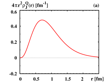
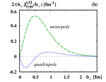
Figure 1: (a) 3D Breit-frame density $\rho_{J}^{Q}(r)$ (solid line) which determines the 3D monopole contribution to the angular momentum density via Eq. (10) and the 3D quadrupole contribution via Eqs. (11, 15). (b) The 2D lightcone densities of the monopole (dashed line) and quadrupole (dotted line) contributions, $J_{\rm mono}^{z,Q}(b_{\perp})$ and $J_{\rm quad}^{z,Q}(b_{\perp})$, which are determined by means of Eq. (20). The densities satisfy $\int\!{\rm d}^{3}r\;\rho_{J}^{Q}(r)=\frac{1}{2}$, $\int\!{\rm d}^{2}b_{\perp}J_{\rm mono}^{z,Q}(b_{\perp})=\frac{1}{2}$ and $\int\!{\rm d}^{2}b_{\perp}J_{\rm quad}^{z,Q}(b_{\perp})=0$.

In order to have a feeling how these densities look like, we use results from the chiral quark soliton model Goeke:2007fp which predicts $\langle r_{J}^{2}\rangle/\langle r^{2}_{\rm ch}\rangle\approx 1.5$ where $\langle r_{J}^{2}\rangle=\int\!{\rm d}^{3}r\,r^{2}\rho_{J}(r)/\int\!{\rm d}^{3}r\,\rho_{J}(r)$ is the mean square radius of the density $\rho_{J}(r)$ and $\langle r_{\rm ch}^{2}\rangle$ is the proton mean square radius defined analogously. In this model the total form factor $J^{Q}(t)$, $Q=u+d$, can be approximated by the analytic expression (21). The numerical result for $\rho_{J}(r)$ from Goeke:2007fp are reasonably approximated by the analytic form (22) in the range $0.3\lesssim r\lesssim 1.5\,{\rm fm}$ with $M\approx 0.83\,{\rm GeV}$. This is sufficient for our purposes to visualize the main features. The result for $\rho_{J}(r)$ from Eq. (22) is shown in Fig. 1a. The results for the 2D densities (20) are generic, see Fig 1b. Similar results were obtained for $J_{\rm mono}^{z,Q}(b_{\perp})$ and $J_{\rm quad}^{z,Q}(b_{\perp})$ in a scalar diquark model in Ref. Lorce:2017wkb . The main quantitative difference is that the results based on the chiral quark soliton, Fig. 1b, are much softer at small $b_{\perp}$ compared to the results from Ref. Lorce:2017wkb . This is presumably due to the fact that the diquark model essentially describes the nucleon structure in terms of a hard perturbative nucleon-quark-diquark vertex, while the results from Ref. Goeke:2007fp are due to soft chiral interactions.

IX Conclusions

It was shown that the monopole and quadrupole contributions to the Breit-frame 3D angular momentum density of the Belifante-improved EMT are not independent of each other, but are characterized in terms of a density $\rho^{a}_{J}(r)$ normalized as $\sum_{a}\int\!{\rm d}^{3}r\;\rho^{a}_{J}(r)=\frac{1}{2}$. This due to the fact that the information content of one Lorentz-scalar form factor, like $J^{a}(t)$, is in one-to-one correspondence to one 3D density defined in the Breit frame, say $\rho^{a}_{J}(r)$. The polarization axis of the nucleon spin breaks spherical symmetry. This induces a quadrupole contribution which, however, contains no independent information, and is uniquely related to the monopole contribution. This is analog to the case of the mechanical densities, pressure $p(r)$ and shear forces $s(r)$, which are derived from the same form factor $D(t)$ and hence also not independent but related to each other by a differential equation following from EMT conservation Polyakov:2002yz .

The monopole and induced quadrupole components are nevertheless both essential for the visualization of the angular momentum density $J^{i,a}(\vec{r},\vec{s})$ as a 3D vector field. The 2D monopole and quadrupole densities in elastic frames Lorce:2017wkb , or equivalently on the lightcone in the Drell-Yan frame Burkardt:2000za ; Lorce:2017wkb , are expressed through integral relations in terms of $\rho_{J}^{a}(r)$. In this work we focused on the Belifante-improved angular momentum density, but the same result holds also for the monopole and quadrupole contributions to several other densities defined in Ref. Lorce:2017wkb .

This result is of importance for two reasons. First, it clarifies which information about the spatial distribution of the nucleon spin is independent, and which can be expressed in terms of other densities. Second, it is model-independent. This provides a valuable test and is worth exploring in models Wakamatsu:2006dy ; Goeke:2007fq ; Cebulla:2007ei ; Grigoryan:2007vg ; Pasquini:2007xz ; Hwang:2007tb ; Abidin:2008hn ; Brodsky:2008pf ; Burkardt:2008ua ; Abidin:2009hr ; Kim:2012ts ; Jung:2014jja ; Kanazawa:2014nha ; Chakrabarti:2015lba ; Mondal:2016xsm ; Adhikari:2016dir ; Kumar:2017dbf ; Mondal:2017lph , lattice QCD Mathur:1999uf ; Hagler:2003jd ; Gockeler:2003jfa ; Hagler:2007xi ; Engelhardt:2017miy ; Bali:2018zgl and effective chiral theories Granados:2019zjw .

Acknowledgments. We are grateful to C. Lorcé, L. Mantovani, B. Pasquini and M. V. Polyakov for valuable discussions and comments on the manuscript. This work was supported by NSF grant no. 1812423 and DOE grant no. DE-FG02-04ER41309.

References

-
(1)
I. Y. Kobzarev and L. B. Okun,
Zh. Eksp. Teor. Fiz. 43, 1904 (1962)
[Sov. Phys. JETP 16, 1343 (1963)].
H. Pagels, Phys. Rev. 144, 1250 (1966). -
(2)
D. Müller, D. Robaschik, B. Geyer, F.-M. Dittes and J. Hořejši,
Fortsch. Phys. 42, 101 (1994).
X. D. Ji, Phys. Rev. Lett. 78, 610 (1997); Phys. Rev. D 55, 7114 (1997);
A. V. Radyushkin, Phys. Lett. B 380, 417 (1996); Phys. Lett. B 385, 333 (1996).
J. C. Collins, L. Frankfurt and M. Strikman, Phys. Rev. D 56, 2982 (1997). -
(3)
X. D. Ji,
J. Phys. G 24, 1181 (1998).
A. V. Radyushkin,
arXiv:hep-ph/0101225.
K. Goeke, M. V. Polyakov and M. Vanderhaeghen, Prog. Part. Nucl. Phys. 47, 401 (2001).
M. Diehl, Phys. Rept. 388 (2003) 41. A. V. Belitsky and A. V. Radyushkin, Phys. Rept. 418, 1 (2005).
S. Boffi and B. Pasquini, Riv. Nuovo Cim. 30, 387 (2007).
M. Guidal, H. Moutarde and M. Vanderhaeghen, Rept. Prog. Phys. 76, 066202 (2013).
K. Kumerički, S. Liuti and H. Moutarde, Eur. Phys. J. A 52 (2016) 157. - (4) M. V. Polyakov, Phys. Lett. B 555, 57 (2003).
- (5) K. Goeke, J. Grabis, J. Ossmann, M. V. Polyakov, P. Schweitzer, A. Silva and D. Urbano, Phys. Rev. D 75, 094021 (2007).
- (6) C. Lorcé, L. Mantovani and B. Pasquini, Phys. Lett. B 776, 38 (2018).
- (7) M. V. Polyakov and P. Schweitzer, Int. J. Mod. Phys. A 33, 1830025 (2018).
- (8) M. V. Polyakov and H. D. Son, JHEP 1809, 156 (2018).
- (9) V. D. Burkert, L. Elouadrhiri, and F. X. Girod, Nature 557, 396 (2018).
- (10) C. Lorcé, H. Moutarde and A. P. Trawiński, Eur. Phys. J. C 79, 89 (2019).
- (11) P. E. Shanahan and W. Detmold, Phys. Rev. Lett. 122, 072003 (2019).
- (12) M. V. Polyakov and P. Schweitzer, arXiv:1812.06143 [hep-ph].
- (13) E. Leader and C. Lorcé, Phys. Rept. 541, 163 (2014).
- (14) M. Wakamatsu, Int. J. Mod. Phys. A 29, 1430012 (2014).
- (15) K. F. Liu and C. Lorcé, Eur. Phys. J. A 52, 160 (2016).
- (16) A. Deur, S. J. Brodsky and G. F. De Téramond, arXiv:1807.05250 [hep-ph].
- (17) X. D. Ji, Phys. Rev. Lett. 74, 1071 (1995); Phys. Rev. D 52, 271 (1995).
- (18) C. Lorcé, Eur. Phys. J. C 78, 120 (2018).
- (19) Y. Hatta and D. L. Yang, Phys. Rev. D 98, 074003 (2018).
- (20) M. B. Voloshin and V. I. Zakharov, Phys. Rev. Lett. 45, 688 (1980).
- (21) V. A. Novikov and M. A. Shifman, Z. Phys. C 8, 43 (1981).
- (22) T. Sugiura, Y. Ikeda and N. Ishii, EPJ Web Conf. 175, 05011 (2018); arXiv:1905.03934 [nucl-th].
- (23) M. V. Polyakov and P. Schweitzer, Phys. Rev. D 98, 034030 (2018).
- (24) S. Dubynskiy and M. B. Voloshin, Phys. Lett. B 666, 344 (2008). A. Sibirtsev and M. B. Voloshin, Phys. Rev. D 71, 076005 (2005). X. Li and M. B. Voloshin, Mod. Phys. Lett. A 29, 1450060 (2014).
- (25) M. I. Eides, V. Y. Petrov and M. V. Polyakov, Phys. Rev. D 93, 054039 (2016); Eur. Phys. J. C 78, 36 (2018); arXiv:1904.11616 [hep-ph].
-
(26)
I. A. Perevalova, M. V. Polyakov and P. Schweitzer,
Phys. Rev. D 94, 054024 (2016).
J. Y. Panteleeva, I. A. Perevalova, M. V. Polyakov and P. Schweitzer, Phys. Rev. C 99, 045206 (2019). - (27) W. Cosyn, S. Cotogno, A. Freese and C. Lorcé, arXiv:1903.00408 [hep-ph].
- (28) M. V. Polyakov and B. D. Sun, arXiv:1903.02738 [hep-ph].
- (29) S. Cotogno, C. Lorcé, P. Lowdon, arXiv:1905.11969 [hep-th].
- (30) M. V. Polyakov and C. Weiss, Phys. Rev. D 60, 114017 (1999).
- (31) R. G. Sachs, Phys. Rev. 126, 2256 (1962).
- (32) J. Hudson and P. Schweitzer, Phys. Rev. D 96, 114013 (2017).
- (33) M. Burkardt, Phys. Rev. D 62, 071503 (2000), Erratum: ibid. 66, 119903 (2002); Int. J. Mod. Phys. A 18, 173 (2003).
- (34) M. Wakamatsu and Y. Nakakoji, Phys. Rev. D 74, 054006 (2006).
- (35) K. Goeke, J. Grabis, J. Ossmann, P. Schweitzer, A. Silva and D. Urbano, Phys. Rev. C 75, 055207 (2007).
- (36) C. Cebulla, K. Goeke, J. Ossmann and P. Schweitzer, Nucl. Phys. A 794, 87 (2007).
- (37) H. R. Grigoryan and A. V. Radyushkin, Phys. Lett. B 650, 421 (2007).
- (38) B. Pasquini and S. Boffi, Phys. Lett. B 653, 23 (2007).
- (39) D. S. Hwang and D. Mueller, Phys. Lett. B 660, 350 (2008).
- (40) Z. Abidin and C. E. Carlson, Phys. Rev. D 77, 115021 (2008).
- (41) S. J. Brodsky and G. F. de Teramond, Phys. Rev. D 78, 025032 (2008).
- (42) M. Burkardt and H. BC, Phys. Rev. D 79, 071501 (2009).
- (43) Z. Abidin and C. E. Carlson, Phys. Rev. D 79, 115003 (2009).
- (44) H. C. Kim, P. Schweitzer and U. Yakhshiev, Phys. Lett. B 718, 625 (2012).
- (45) J. H. Jung, U. Yakhshiev, H. C. Kim and P. Schweitzer, Phys. Rev. D 89, 114021 (2014).
- (46) K. Kanazawa, C. Lorcé, A. Metz, B. Pasquini and M. Schlegel, Phys. Rev. D 90, 014028 (2014).
- (47) D. Chakrabarti, C. Mondal and A. Mukherjee, Phys. Rev. D 91, 114026 (2015).
- (48) C. Mondal, N. Kumar, H. Dahiya and D. Chakrabarti, Phys. Rev. D 94, 074028 (2016).
- (49) L. Adhikari and M. Burkardt, Phys. Rev. D 94, 114021 (2016).
- (50) N. Kumar, C. Mondal and N. Sharma, Eur. Phys. J. A 53, 237 (2017).
- (51) C. Mondal, D. Chakrabarti and X. Zhao, Eur. Phys. J. A 53, 106 (2017).
- (52) N. Mathur, S. J. Dong, K. F. Liu, L. Mankiewicz and N. C. Mukhopadhyay, Phys. Rev. D 62, 114504 (2000)
- (53) P. Hägler et al. [LHPC and SESAM Collaborations], Phys. Rev. D 68, 034505 (2003) [hep-lat/0304018].
- (54) M. Göckeler et al. [QCDSF Collaboration], Phys. Rev. Lett. 92, 042002 (2004) [hep-ph/0304249].
- (55) P. Hägler et al. [LHPC Collaboration], Phys. Rev. D 77, 094502 (2008).
- (56) M. Engelhardt, Phys. Rev. D 95, 094505 (2017).
- (57) G. S. Bali, S. Collins, M. Göckeler, R. Rödl, A. Schäfer and A. Sternbeck, arXiv:1812.08256 [hep-lat].
- (58) C. Granados and C. Weiss, arXiv:1905.02742 [hep-ph].