Adversarial Imitation Learning from Incomplete Demonstrations

Abstract

Imitation learning targets deriving a mapping from states to actions, a.k.a. policy, from expert demonstrations. Existing methods for imitation learning typically require any actions in the demonstrations to be fully available, which is hard to ensure in real applications. Though algorithms for learning with unobservable actions have been proposed, they focus solely on state information and overlook the fact that the action sequence could still be partially available and provide useful information for policy deriving. In this paper, we propose a novel algorithm called Action-Guided Adversarial Imitation Learning (AGAIL) that learns a policy from demonstrations with incomplete action sequences, i.e., incomplete demonstrations. The core idea of AGAIL is to separate demonstrations into state and action trajectories, and train a policy with state trajectories while using actions as auxiliary information to guide the training whenever applicable. Built upon the Generative Adversarial Imitation Learning, AGAIL has three components: a generator, a discriminator, and a guide. The generator learns a policy with rewards provided by the discriminator, which tries to distinguish state distributions between demonstrations and samples generated by the policy. The guide provides additional rewards to the generator when demonstrated actions for specific states are available. We compare AGAIL to other methods on benchmark tasks and show that AGAIL consistently delivers comparable performance to the state-of-the-art methods even when the action sequence in demonstrations is only partially available.

1 Introduction

Imitation learning is a framework for learning a behavior policy from demonstrations. Usually, demonstrations are presented in the form of state-action trajectories, with each pair indicating the action to take at the state being visited. In order to learn the behavior policy, the demonstrated actions are usually utilized in two ways. The first, known as Behavior Cloning (BC) Bain and Sommut (1999), treats the action as the target label for each state, and then learns a generalized mapping from states to actions in a supervised manner Pomerleau (1991). Another way, known as Inverse Reinforcement Learning (IRL) Ng et al. (2000), views the demonstrated actions as a sequence of decisions, and aims at finding a reward/cost function under which the demonstrated decisions are optimal. Once the reward/cost function is found, the policy could then be obtained through a standard Reinforcement Learning algorithm.

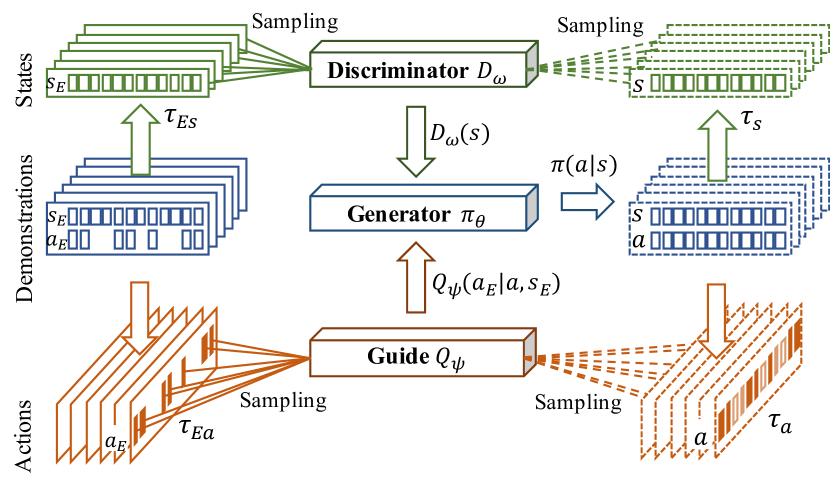
Figure 1: Action-Guided Adversarial Imitation Learning has three components: a generator, a discriminator, and a guide. The discriminator distinguishes state distributions between demonstrations and samples generated by the generator, i.e., policy. The guide provides auxiliary rewards to the generator whenever actions are available.

Nevertheless, both BC and IRL algorithms implicitly assume that the demonstrations are complete, meaning that the action for each demonstrated state is fully observable and available  Gao et al. (2018). This assumption hardly holds for a real imitation learning task. First, the actions (not the states) in demonstrations may be partially observable or even unobservable Torabi et al. (2018). For example, when showing a robot how to correctly lift up a cup, the demonstrator’s states – body movements – can be visually captured but the human actions – the force and torque applied to the body joint – are unavailable to the robot Eysenbach et al. (2018). Furthermore, even if the actions are obtainable, some of them may be invalid and need to be eliminated from learning due to the demonstrator’s individual factors Argall et al. (2009), e.g., the expertise level or strategy preferences Li et al. (2017) Without complete action information in demonstrations, the conventional BC and IRL algorithms are unable to produce the desired policy.

Though some recent studies have proposed to use state trajectories Merel et al. (2017) or recover actions from state transitions Torabi et al. (2018) for imitation learning, they rely solely on state information, and largely overlook the fact that a partial action sequence could still be available in one demonstration. It is thus necessary to design an algorithm that could handle demonstrations with partial action sequences.

To this end, we propose a novel algorithm, Action-Guided Adversarial Imitation Learning (AGAIL), that can be applied to demonstrations with incomplete action sequences. The main idea of AGAIL algorithm is to divide the state-action pairs in demonstrations into state trajectories and action trajectories, and learns a policy from states with auxiliary guidance from actions, if available. To be more specific, AGAIL is built on adversarial imitation, an idea of training a policy by competing it with a discriminator, which tries to distinguish between state-action pairs from expert as opposed to from the policy Ho and Ermon (2016). AGAIL further divides the state-action matching into two components, state matching and action guidance, and simultaneously maintains three networks: a generator, a discriminator, and a guide, as shown in Figure 1. The generator generates a policy via a state-of-the-art policy gradient method; the discriminator distinguishes the state distribution between demonstrations and the learned policy, and assigns rewards to the generator; and the guide provides additional credits by maximizing the mutual information between generated actions and demonstrated actions if available. The policy net and the state discrimination net are trained by competing with each other, while the action guidance net is trained only when actions for specific states are available. We present a theoretical analysis of AGAIL to show its correctness. Through various experiments on different levels of incompleteness of actions in demonstrations, we show that AGAIL consistently delivers comparable performance to two state-of-the-art algorithms even when the demonstrations provided are incomplete.

2 Related Work

This section briefly introduces imitation learning algorithms, and then discusses how demonstrations with partial or unobservable actions are handled by previous studies.

To solve an imitation learning problem, one simple yet effective method is Behavior Cloning (BC) Bain and Sommut (1999), a supervised learning approach that directly learns a mapping from states to actions from demonstrated data Ross and Bagnell (2010). Though successfully applied to various applications, e.g., autonomous driving Bojarski et al. (2016) and drone flying Daftry et al. (2016), BC suffers greatly from the compounding error, a situation where minor errors are compounded over time and finally induce a dramatically different state distribution Ross et al. (2011). Another approach, Inverse Reinforcement Learning (IRL) Ng et al. (2000), aims at searching for a reward/cost function that could best explain the demonstrated behavior. Yet the function search is ill-posed as the demonstrated behavior could be induced by multiple reward/cost functions. Constraints are thereby imposed on the rewards or the policy to ensure the optimality uniqueness of the demonstrated behavior. For example, the reward function is usually defined to be a linear Ng et al. (2000); Abbeel and Ng (2004) or convex Syed et al. (2008) combination of the state features. The learned policy is also assumed to have the maximum entropy Ziebart et al. (2008) or the maximum causal entropy ziebart2010casual_entropy. These explicit constraints, on the other hand, potentially limit the generability of the proposed methods Ho and Ermon (2016). Only recently, Finn et al. have proposed to skip the reward constraints and used demonstrations as an implicit guidance for reward searching Finn et al. (2016). Nevertheless, the reward-based methods are computationally intensive and hence are limited to simple applications Ho and Ermon (2016). To address this issue, Generative Adversarial Imitation Learning (GAIL) Ho and Ermon (2016) was proposed to use a discriminator to distinguish whether a state-action pair is from an expert or from the learned policy. Since GAIL has achieved state-of-the-art performance in many applications, we thus derive our algorithms based on the GAIL method. For more details on GAIL, refer to Prelminary.

The aforementioned algorithms, however, can hardly handle the demonstrations with partial or unobservable actions. One idea to learning from these demonstrations is to first recover actions from states and then adopt standard imitation learning algorithms to learn a policy from the recovered state-action pairs. For example, Torabi et al. recovered actions from states by learning a dynamic model of state transitions, and then use a BC algorithm to find the optimal policy Torabi et al. (2018). However, the performance of this method is highly dependent on the learned dynamic model, and may fail when the states transit with noise. Instead, Merel et al. proposed to learn from only state (or state feature) trajectories. They extended the GAIL framework to learn a control policy from only states of motion capture demonstrations Merel et al. (2017), and showed that partial state features without demonstrator actions suffice for adversarial imitation. Similarly, Eysenbach et al. pointed out that the policy should control which states the agent visits, and thus used states to train a policy by maximizing mutual information between the policy and the state trajectories Eysenbach et al. (2018). Other studies have also tried to learn from raw observations, instead of states. For instance, Stadie et al. extracted features from observations by the domain adaptation method to ensure that experts and novices are in the same feature space Stadie et al. (2017). However, only using demonstrated states or state features may require a huge number of environmental interactions during the training since any possible information from actions is ignored.

3 Preliminary

An infinite-horizon, discounted Markov Decision Process (MDP) is modeled by tuple $(\mathcal{S},\mathcal{A},P,r,\rho_{0},\gamma)$, where $\mathcal{S}$ is the state space, $\mathcal{A}$ is the action space, $P:\mathcal{S}\times\mathcal{A}\times\mathcal{S}\rightarrow\mathbb{R}$ denotes the state transition probability, $r:\mathcal{S}\times\mathcal{A}\rightarrow\mathbb{R}$ represents the reward function, $\rho_{0}:\mathcal{S}\rightarrow\mathcal{A}$ is the initial state distribution, and $\gamma\in(0,1]$ is a discount factor. A stochastic policy $\pi\in\Pi$ is $\pi:\mathcal{S}\times\mathcal{A}\rightarrow[0,1]$. Let $\tau_{E}$ denote a trajectory sampled from expert policy $\pi_{E}$: $\tau_{E}=\big{[}(s_{0},a_{0}),(s_{1},a_{1}),...,(s_{n},a_{n})\big{]}$. We also use $\tau_{Es}$ and $\tau_{Ea}$ to denote state component and action component in $\tau_{E}$: $\tau_{E}=(\tau_{Es},\tau_{Ea})$, $\tau_{Es}=[s_{0},s_{1},...,s_{n}]$ and $\tau_{Ea}=[a_{0},a_{1},...,a_{n}]$. We use the expectation with respect to a policy $\pi$ to denote an expectation with respect to trajectories it generates: $\mathbb{E}_{\pi}\big{[}r(s,a)\big{]}\triangleq\mathbb{E}\big{[}\sum_{t=0}^{\infty}\gamma^{t}r(s_{t},a_{t})\big{]}$, where $s_{0}\sim\rho_{0}$, $a_{t}\sim\pi(a_{t}|s_{t})$, $s_{t+1}\sim P(s_{t+1}|a_{t},s_{t})$.

To address the imitation learning problem, we adopt the apprenticeship learning formalism Abbeel and Ng (2004): the learner finds a policy $\pi$ that performs not worse than expert $\pi_{E}$ with respect to an unknown reward function $r(s,a)$. We define the occupancy measure $\rho_{\pi}\in\mathcal{D}:\mathcal{S}\times\mathcal{A}\rightarrow\mathbb{R}$ of a policy $\pi\in\Pi$ as: $\rho_{\pi}(s,a)=\pi(a|s)\sum_{t=0}^{\infty}\gamma^{t}p(s_{t}=s|\pi)$ Puterman (2014). Owing to the one-to-one correspondence between $\Pi$ and $\mathcal{D}$, an imitation learning problem is equivalent to a matching problem between $\rho_{\pi}(s,a)$ and $\rho_{\pi_{E}}(s,a)$. A general objective of imitation learning is

$$\arg\min_{\pi\in\Pi}-\lambda_{1}H(\pi)+\psi^{*}(\rho_{\pi}-\rho_{\pi_{E}})$$ (1)

where $H(\pi)\triangleq\mathbb{E}_{\pi}\big{[}-\log\pi(s,a)\big{]}$, is the $\gamma$-discounted causal entropy of the policy $\pi(s,a)$, and $\psi^{*}$ is a distance measure between $\rho_{\pi}$ and $\rho_{\pi_{E}}$. In GAIL framework, the distance measure is defined as follows:

$$\psi_{GA}^{*}(\rho_{\pi}-\rho_{\pi_{E}})=\max_{D}\mathbb{E}_{\pi}\big{[}\log D\big{]}+\mathbb{E}_{\pi_{E}}\big{[}\log(1-D)\big{]}$$ (2)

where $D\in(0,1)^{\mathcal{S}\times\mathcal{A}}$ is a discriminator with respect to state-action pairs. Based on this formalism, imitation learning becomes training a generator against a discriminator: generator $\pi_{\theta}$ generates state-action pairs while the discriminator tries to distinguish them from demonstrations. The optimal policy is learned when the discriminator fails to draw a distinction.

Problem formulation.

We now formulate the problem of imitation learning from incomplete demonstrations. Without loss of generality, we define a demonstration to be incomplete based on the action condition: a demonstration $\tau_{E}$ is said to be incomplete if part(s) of its action component $\tau_{Ea}$ is missing, i.e., $|\tau_{Ea}|\leq|\tau_{Es}|$. Figure 1 illustrates $\tau_{Es}$ and $\tau_{Ea}$ in an incomplete demonstration. Then imitation learning from incomplete demonstrations becomes the learner finds a policy $\pi$ that performs not worse than the expert $\pi_{E}$, which is provided in state trajectory samples and action trajectory samples, i.e., $\tau_{Es}=\{\tau_{Es}^{i}\}$, $\tau_{Ea}=\{\tau_{Ea}^{i}\}$ and $|\tau_{Ea}^{i}|\leq|\tau_{Es}^{i}|\quad\forall i$.

4 Action-Guided Adversarial Imitation

We now describe our imitation learning algorithm, AGAIL, which combines state-based adversarial imitation with action-guided regularization. Motivated by the studies on utilizing demonstrations to steer explorations in Reinforcement Learning Brys et al. (2015); Kang et al. (2018), we propose to separate the demonstrations into two parts: state trajectories and action trajectories. The state trajectories $\tau_{Es}=\{\tau_{Es}^{i}\}$ are for learning an optimal policy, while the action trajectories $\tau_{Ea}=\{\tau_{Ea}^{i}\}$ provides auxiliary information to shape the learning process. AGAIL has two parts: a state-based adversarial imitation, and an action-guided regularization. The pseudo-code of AGAIL is given in Algorithm 1.

Algorithm 1 Action-guided adversarial imitation learning

Input: expert trajectories $\tau_{E}=\{(\tau_{Es}^{i},\tau_{Ea}^{i})\}\sim\pi_{E}$
Parameter: Policy, discriminator and posterior parameters $\theta_{0}$, $\omega_{0}$, $\psi_{0}$; hyperparameters $\alpha$ and $\beta$
Output: Learned policy $\pi_{\theta}$

  for $i=0,1,2,...$ do

     Sample trajectories: $\tau^{i}\sim\pi_{\theta_{i}}$ during each rollout.

     Sample states $s^{i}\sim\tau_{s}^{i}$, $s_{E}^{i}\sim\{\tau_{Es}^{i}\}$ by same batch size.

     Update $\omega_{i}$ to $\omega_{i+1}$ for $D_{\omega}$ based on Equation 4.

     Query $\{a_{E}^{i}\}$ and run $\pi_{\theta_{i}}$ on $\{s_{E}^{i}\}$ to collect $\{a^{i}\}$.

     Update $\psi_{i}$ to $\psi_{i+1}$ for $Q_{\psi}$ based on Equation 5.

     Update $\theta_{i}$ to $\theta_{i+1}$ via TRPO for Equation 4.2 with rewards $r(s,a)=\alpha D_{\omega_{i+1}}(s)+\beta Q_{\psi_{i+1}}(a_{E}|s,a)\quad a_{E}\sim\tau_{Ea}$

  end for

4.1 State-Based Adversarial Imitation

We start from the occupancy measure matching Littman et al. (1995); Ho and Ermon (2016) in imitation learning and show that a policy $\pi$ can be learned from state trajectories $\{\tau_{Es}\}$, which we called state-based adversarial imitation. In general, any imitation learning problem can be converted into a specific matching problem between two occupancy measures: one with respect to the expert policy, $\rho_{\pi_{E}}(s,a)$, and another with respect to the learned policy, $\rho_{\pi}(s,a)$ Pomerleau (1991). However, $\rho_{\pi_{E}}(s,a)$ cannot be calculated exactly since the expert demonstrations are only provided in the form of a finite set of trajectories. Thus the matching of two occupancy measures is further relaxed into a regularization as shown in Equation 1, with $\psi$ penalizes the difference between the two occupancy measures. It has been shown that many imitation learning algorithms, e.g., apprenticeship learning methods Abbeel and Ng (2004); Syed et al. (2008), are actually originated from some specific variant of this regularizer Ho and Ermon (2016). Hence, we derive our algorithm based on Equation 1.

To optimize Equation 1, both states and actions need to be available in demonstrations, especially for the second term $\psi^{*}(\rho_{\pi}-\rho_{\pi_{E}})$ (the first term is constant if we define the policy to be Gaussian). Ho and Ermon have demonstrated that, if we choose the $\psi^{*}$ to be $\psi_{GA}^{*}$ in Equation 2, then $D\in(0,1)$ relies only on rewards $r(s,a)$, and can be defined as a special function of $(s,a)$ Ho and Ermon (2016). Thus, after choosing $\psi$, the definition of $r$ determines the form of $D$. In many practical applications, the reward $r$ is defined based solely on states. For example, when training a human skeleton to walk in a simulation environment, the reward is defined mainly on the body positions and velocities, i.e., states. This is partly because the observed state trajectories are sufficiently invariant across a human skeleton Merel et al. (2017).

We now show that $\psi^{*}(\rho_{\pi}-\rho_{\pi_{E}})$ can be approximated by another distance measure that is defined only on states. Assuming the reward $r$ is defined (mainly) on states $s$ and $\psi^{*}=\psi_{GA}^{*}$, we can now define $D$ as $D(s)\in(0,1)$, a function with respect to states only. Let $\nu(s)$ denote the state visitations $\nu(s)=\sum_{t=0}^{\infty}\gamma^{t}p(s_{t}=s|\pi)$. Accordingly, the occupancy measure $\rho_{\pi}(s,a)$ can be written as $\rho_{\pi}(s,a)=\pi(a|s)\nu_{\pi}(s)$. Equation 2 now becomes

$$\max_{D\in(0,1)}\mathbb{E}_{\pi}\big{[}\log D(s,a)\big{]}+\mathbb{E}_{\pi_{E}}\big{[}\log(1-D(s,a))\big{]}$$

$$\approx \max_{D\in(0,1)}\mathbb{E}_{\pi}\big{[}\log D(s)\big{]}+\mathbb{E}_{\pi_{E}}\big{[}\log(1-D(s))\big{]}$$

$$= \sum_{s,a}\max_{D}\rho_{\pi}(s,a)\log D(s)+\rho_{\pi_{E}}(s,a)\log(1-D(s))$$

$$= \sum_{s,a}\max_{D}\leavevmode\resizebox{346.89731pt}{}{$\pi(a|s)\nu_{\pi}(s)\log D(s)+\pi_{E}(a|s)\nu_{E}(s)\log(1-D(s))$}$$

$$= \sum_{s}\max_{D\in(0,1)}\nu_{\pi}(s)\log D(s)+\nu_{E}(s)\log(1-D(s))$$

$$= \max_{D}\mathbb{E}_{s\sim\pi}\log D(s)+\mathbb{E}_{s\sim\pi_{E}}\log(1-D(s))$$ (3)

This equation implies that, rather than matching the distribution of state-action pairs, we can instead compare the state distribution with the demonstrations to train an optimal policy. Similar to GAIL framework, we train a discriminator $D(s)$ to distinguish the state distribution between the generator and the true data. When $D(s)$ cannot distinguish the generated data from the true data, then $\pi$ has successfully matched the true data. In this setting, the learner’s state visitations $\nu_{\pi}(s)$ is analogous to the data distribution from the generator, and the expert’s state visitations $\nu_{\pi_{E}}$ is analogous to the true data distribution. We now introduce a discriminator network $D_{\omega}:\mathcal{S}\rightarrow(0,1)$, with weights $\omega$, and update it on $\omega$ to maximize Equation 4.1 with the following gradient.

$$\mathbb{E}_{s}\big{[}\nabla_{\omega_{i}}\log D_{w_{i}}(s)\big{]}+\mathbb{E}_{s_{E}}\big{[}\nabla_{\omega_{i}}\log(1-D_{w_{i}}(s))\big{]}$$ (4)

We also parametrize the policy $\pi$, i.e., the generator, with weight $\theta$, and optimize it with Trust Region Policy Optimization (TRPO) Schulman et al. (2015) as it changes the policy $\pi_{\theta}$ within small trust region to avoid policy collapse. The generator $\pi_{\theta}$ and the discriminator $D_{\omega}(s)$ forms the structure of state-based adversarial imitation.

4.2 Action-Guided Regularization

One downside of the state-based adversarial imitation described above is the lack of considering any available actions in demonstrations. Although incomplete and partially available, these action sequences can still provide useful information for the policy learning and explorations Kang et al. (2018). We now considers how to utilize the partial actions in demonstrations. One technique that is widely adopted in Learning from Demonstration is reward shaping Ng et al. (1999); Brys et al. (2015), i.e., defining potentials for demonstrated actions to modify rewards. However, the definition of an appropriate potential function for demonstrated actions is non-trivial, especially when the actions are continuous and high-dimensional. We instead borrow the idea from InfoGAN Chen et al. (2016) and InfoGAIL Li et al. (2017) to incorporate demonstrated actions into learning process by information theories. In particular, there should be high mutual information between two distributions: the demonstrated actions $a_{E}$ and the generated actions $a\sim\pi(s_{E})$ for any specific state $s_{E}$ that corresponds to the demonstrated actions. In information theory, mutual information between $a_{E}$ and $a\sim\pi(s_{E})$, $I(a_{E};a\sim\pi(s_{E}))$, measures the “amount of information” provided to $a_{E}$ when knowing $a\sim\pi(s_{E})$. In other words, $I(a_{E};a\sim\pi(s_{E}))$ is the reduction of uncertainties in $a_{E}$ when $a\sim\pi(s_{E})$ is observed. Thus, we formulate an additional regularizer for the training objective: given any $a_{E}\in\{\tau_{Ea}\}$, we want $I(a_{E}|a\sim\pi(s_{E})$ to have maximum mutual information, where $s_{E}$ is the state where the action $a_{E}$ is demonstrated, and $a$ is sampled from $\pi(s_{E})$.

However, the mutual information is hard to maximize as it requires the posterior $P(a_{E}|a\sim\pi(s_{E}))$. We adopt the same idea in InfoGAIL to introduce a variational lower bound, $L_{I}(\pi,Q)$, of the mutual information $I(a_{E};a\sim\pi(s_{E}))$:

$$L_{I}(\pi,Q) =\mathbb{E}_{a_{E}\sim\{\tau_{Ea}\}}\big{[}\log Q(a_{E}|a,s_{E})\big{]}+H(a_{E})$$

$$\leq I\big{(}a_{E};a\sim\pi(s_{E})\big{)}$$

where $Q(a_{E}|a,s_{E})$ is an approximation of the true posterior $P(a_{E}|a\sim\pi(s_{E}))$. We parameterize the posterior approximation $Q$ with weights $\psi$, i.e., $Q_{\psi}(a_{E}|a,s_{E})$, by a neural network and update $Q_{\psi}$ by the following gradients:

$$-\mathbb{E}_{s_{E},a_{E}}\big{[}\nabla_{\psi_{i}}\log Q_{\psi_{i}}(a_{E}|a,s_{E})\big{]}$$ (5)

Note that the mutual information is maximized between the distribution of demonstrated actions and the distribution of generated actions from the same state. The weights of $Q$ are shared across all demonstrated actions and states.

Env.	$\mathcal{S}\times\mathcal{A}$	Empirical Return
		TRPO	GAIL	State	AGAIL.00	AGAIL.25	AGAIL.50	AGAIL.75
CartPole	$\mathbb{R}^{4}\times\{0,1\}$	196.4±2	188.6±6	188.3±8	18.4±1	197.2±1	193.6±5	197.9±1
Hopper	$\mathbb{R}^{11}\times\mathbb{R}^{3}$	2.6e3±96	2.5e3±181	2.6e3±203	1.0e3±23	1.4e3±269	1.5e3±309	2.7e3±131
Walker2d	$\mathbb{R}^{17}\times\mathbb{R}^{6}$	2.4e3±180	2.3e3±280	2.0e3±121	2.3e3±84	2.6e3±150	2.3e3±109	2.2e3±200
Humanoid	$\mathbb{R}^{376}\times\mathbb{R}^{17}$	523.9±8	509.2±14	544.7±12	586.4±14	571.3±10	548.6±12	542.3±6

Table 1: Environment specifications and numerical results.

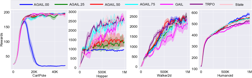
Figure 2: Reward curves of AGAIL{.00, 0.25, 0.50, .75}, TRPO, GAIL and state-GAIL ({.xx} denotes the incompleteness ratio).

Now, we present the Action-Guided Adversarial Imitation Learning (AGAIL) algorithm. The learning objective that combines the state-based adversarial imitation and the action-guided regularization is:

$$\min_{\pi\in\Pi}\big{[} -\lambda_{1}H(\pi_{\theta})-\lambda_{2}L_{I}(\pi_{\theta},Q_{\psi})+$$

$$\max_{D}\mathbb{E}_{s\sim\pi_{\theta}}\log D_{\omega}+\mathbb{E}_{s\sim\pi_{E}}\log(1-D_{\omega})\big{]}$$ (6)

where $\lambda_{1},\lambda_{2}>0$ are two hyperparameters for the casual entropy of policy $\pi_{\theta}$ and the mutual information maximization respectively. Optimizing the objective involves three steps: maximizing Equation 4, minimizing Equation 5, and minimizing Equation 4.2 with fixed $D_{\omega_{i}}$ and $Q_{\psi_{i}}$. The first step is similar as GAIL. In second step, we assume that all demonstrated state-action pairs $(s_{E}^{i},a_{E}^{i})$ are independent and only update $Q_{\psi}$ when $a_{E}$ is available for $s_{E}$. When updating $Q_{\psi}$, we use $(a_{E}^{i},a,s_{E}^{i})$, where $a\sim\pi_{\theta}(s_{E})$; when using $Q_{\psi}$ as additional rewards for $(s,a)$, we sample $a_{E}\sim\tau_{Ea}$ and then feed a tuple $(a_{E},a,s)$ to $Q$. To conduct the third-step optimization, we use both $D(s)$ and $Q(a_{E}^{i}|a,s_{E}^{i})$ as rewards to update $\pi_{\theta}$ on state $s_{E}$, i.e., $r(s_{E},a)=\alpha D_{\omega}(s_{E})+\beta Q(a_{E}^{i}|s,a)$ where $\alpha$ and $\beta$ are coefficients. In the experiment, we set $\alpha$ to 1 and relate $\beta$ to the incompleteness ratio $\eta\in(0,1)$ of actions in demonstrations, $\beta=1-\eta$. The three steps are run iteratively until convergence. An outline for this procedure is given in Algorithm 1.

5 Experiment

We want to investigate two aspects of AGAIL: the effectiveness of learning from incomplete demonstrations, and the robustness when the degree of incompleteness changes. Specifically, we compare AGAIL to three algorithms, TRPO, GAIL and state-only GAIL, to show its learning performance. The reason for choosing TRPO is that, given true reward signals, TRPO delivers the state-of-the-art performance, which can then be referred to as the “expert” when the true rewards are unknown. We select GAIL as it is the state-of-the-art for imitation learning when demonstrations are complete. We also adopt state-GAIL Merel et al. (2017) (using states only to train GAIL and equivalent to AGAIL.100) to show the performance boost introduced by action guidance. The characteristics of each algorithm are listed below:

• TRPO: true $r$; no $\tau_{Es}$ and no $\tau_{Ea}$

• GAIL: discriminator $r$; $\tau_{Es}$ and $\tau_{Ea}$

• State-GAIL: discriminator $r$; $\tau_{Es}$ and no $\tau_{Ea}$

• AGAIL: discriminator & guide $r$; $\tau_{Es}$ and partial $\tau_{Ea}$

In addition, we vary the level of incompleteness of demonstrations to showcase the robustness of AGAIL. Four simulation tasks, Cart Pole, Hopper, Walker and Humanoid (from low-dimensional to high-dimensional controls), are selected to cover discrete and continuous state/action space, and the specifications are listed in Table 1. Note that the rewards defined in all four environments are mainly dependent on the states. For example, the rewards for Cart Pole is set as a function of positions and angles of the pole; the rewards for Hopper, Walker and Humanoid all have a significant weight on states Brockman et al. (2016). Thus our assumption that the reward $r$ is (mainly) a function of the state $s$ holds for all experimental environments.

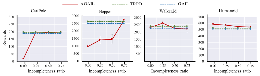
Figure 3: AGAIL performance versus TRPO and GAIL baselines as the incompleteness ratio changes

Implementations.

We use stochastic policy parametrized by three fully connected layers (100 hidden units and Tanh activation), and construct the value network by sharing the layers with the policy network. Both policy net and value net are optimized through gradient descend with Adam optimizer. Demonstrations are collected by running a policy trained via TRPO. We then randomly mask out actions to manipulate the incompleteness with four ratios (0%, 25%, 50%, and 75%): 0% means all the actions are available while 75% means 75% of the actions in each demonstration are masked out. All experiments are run for six times with different initialization seeds (0-5). We use empirical returns to evaluate performance for the learned policy. All algorithms are implemented based on the work Brockman et al. (2016).

5.0.1 Experiment Results

We first compare the performance of AGAIL with TRPO, GAIL and state-GAIL in multiple control tasks. The average accumulated rewards are given in Table 1 and the learning curves are plotted in Figure 2. The numerical results in Table 1 show that AGAIL algorithm achieves learning performance comparable with that of TRPO (true rewards) and GAIL (complete demonstrations), and outperforms state-GAIL. Specifically, in CartPole tasks, AGAIL{.25, .50, .75} all achieve almost the same performance as that of TRPO and GAIL, even if it is trained with incomplete actions. The same phenomenon is observed in Walker2d and Humanoid environments. We also notice that, AGAIL{.00, .25, .50, .75} all outperform state-GAIL in Walker2d and Humanoid. Such performance boost in AGAIL, especially in Humanoid, further shows that the guidance layer is vital for AGAIL. However, in contrast to Walker2d and Humanoid, AGAIL.00 performs poorly in CartPole and Hopper. Such performance drop in CartPole and Hopper may possibly be caused by the qualities of demonstrations, i.e., the extent to whether demonstrations are good samples to show the expected optimal behaviour in expert policy Brys et al. (2015). The TRPO policy of these tasks (especially Hopper), though delivering good results in general, suffers from big performance fluctuations. Any one of the checkpoints from the TRPO policy could be impaired by the fluctuations regardless of its returns. In our experiment, demonstrations are generated by running one selected checkpoint (e.g., the one with the highest return) out of all possible TRPO checkpoints, which may overfit one batch of examples and produce actions that fail to scale. Forcefully requiring the policy actions to share similar distribution of these actions could thus lead to policy collapse.

We are surprised that the AGAIL, trained with incomplete demonstrations, e.g., AGAIL.75, even outperforms GAIL with a noticeable margin in Hopper, Walker2d and Humanoid. Meanwhile, AGAIL{.00, .25, .50} all performs worse than AGAIL.75, especially in Hopper. We also notice that, in the same environment, GAIL fails to deliver satisfying results across all tasks. GAIL, AGAIL{.00, .25, .50} are all trained with a large portion ($\geq 50\%$) of demonstrated actions, while AGAIL.75 and TRPO are trained with much less or no actions. One might wonder why incorporating more actions fail to improve performance. A possible explanation is that demonstrations are limited samples from a training checkpoint (e.g., the one with the highest returns) of an expert policy Ho and Ermon (2016). If the checkpoint itself is from an unstable training process, e.g., TRPO training in Hopper, more demonstrations are likely to introduce more undesirable variances in action distributions Kang et al. (2018), which consequently interferes with policy deriving Ross et al. (2011). The same phenomenon has been observed in Ho and Ermon (2016); Baram et al. (2017). In contrast, if demonstrations are sampled by a checkpoint from a stable training, e.g., TRPO training in Humanoid, employing more actions could lead to better results. As shown in Figure 2 Humanoid, AGAIL performance improves as more actions are utilized. Further, results in Figure 2 Hopper suggest that demonstrations, or more specifically the actions, are not helpful for agents to learn a policy. This highlights the importance of demonstration qualities and the necessity of algorithms to handle incomplete actions.

We then test the robustness of AGAIL. Figure 3 shows how the AGAIL performance changes as the incompleteness ratio increases. We notice that in Hopper and Humanoid, AGAIL consistently obtains more returns than GAIL under different ratios of action incompleteness. It even achieves the highest returns when used to train the Humanoid. However, in Walker2d environment, the returns of AGAIL fluctuate widely. This may possibly be caused by the large variance during the training, as shown in the AGAIL training curves in Walker2d in Figure 2. In all four subfigures, the TRPO algorithm performs stably better than the GAIl. In Hopper environment, the TRPO obtains much higher returns than the GAIL, while, in other environments, they achieve comparable returns. This may further verify the above guess that the demonstrated actions for Hopper are largely suboptimal.

Combining above discussions, we conclude that AGAIL is effective in learning from incomplete demonstrations, and consistently delivers robust performance under different incompleteness ratios of demonstrated actions.

6 Conclusions

We considered imitation learning from demonstrations with incomplete action sequences, and proposed a novel and robust algorithm, AGAIL, to learn a policy from incomplete demonstrations. AGAIL treats states and actions in demonstrations separately. It first uses state trajectories to train a classifier and a discriminator: the classifier tries to distinguish the state distributions of expert demonstrations from the state distributions of generated samples; the discriminator leverages the feedback from the clsssifier to train a policy. Meanwhile, AGAIL also trains a guide to maximize the mutual information between any demonstrated actions, if available, and the policy actions, and assigns additional rewards to the generator. Experiment results suggest that AGAIL consistently delivers comparable performance to the TRPO and GAIL even if trained with incomplete demonstrations.

References

- Abbeel and Ng [2004] Pieter Abbeel and Andrew Y Ng. Apprenticeship learning via inverse reinforcement learning. In ICML, page 1. ACM, 2004.
- Argall et al. [2009] Brenna D Argall, Sonia Chernova, Manuela Veloso, and Brett Browning. A survey of robot learning from demonstration. Robotics and autonomous systems, 57(5):469–483, 2009.
- Bain and Sommut [1999] Michael Bain and Claude Sommut. A framework for behavioural cloning. Machine intelligence, 15(15):103, 1999.
- Baram et al. [2017] Nir Baram, Oron Anschel, Itai Caspi, and Shie Mannor. End-to-end differentiable adversarial imitation learning. In ICML, pages 390–399, 2017.
- Bojarski et al. [2016] Mariusz Bojarski, Davide Del Testa, Daniel Dworakowski, Bernhard Firner, Beat Flepp, Prasoon Goyal, Lawrence D Jackel, Mathew Monfort, Urs Muller, Jiakai Zhang, et al. End to end learning for self-driving cars. arXiv preprint arXiv:1604.07316, 2016.
- Brockman et al. [2016] Greg Brockman, Vicki Cheung, Ludwig Pettersson, Jonas Schneider, John Schulman, Jie Tang, and Wojciech Zaremba. Openai gym. arXiv preprint arXiv:1606.01540, 2016.
- Brys et al. [2015] Tim Brys, Anna Harutyunyan, Halit Bener Suay, Sonia Chernova, Matthew E Taylor, and Ann Nowé. Reinforcement learning from demonstration through shaping. In IJCAI, 2015.
- Chen et al. [2016] Xi Chen, Yan Duan, Rein Houthooft, John Schulman, Ilya Sutskever, and Pieter Abbeel. Infogan: Interpretable representation learning by information maximizing generative adversarial nets. In NeurIPS, pages 2172–2180, 2016.
- Daftry et al. [2016] Shreyansh Daftry, J Andrew Bagnell, and Martial Hebert. Learning transferable policies for monocular reactive mav control. In International Symposium on Experimental Robotics. Springer, 2016.
- Eysenbach et al. [2018] Benjamin Eysenbach, Abhishek Gupta, Julian Ibarz, and Sergey Levine. Diversity is all you need: Learning skills without a reward function. arXiv preprint arXiv:1802.06070, 2018.
- Finn et al. [2016] Chelsea Finn, Sergey Levine, and Pieter Abbeel. Guided cost learning: Deep inverse optimal control via policy optimization. In ICML, pages 49–58, 2016.
- Gao et al. [2018] Yang Gao, Ji Lin, Fisher Yu, Sergey Levine, Trevor Darrell, et al. Reinforcement learning from imperfect demonstrations. arXiv preprint arXiv:1802.05313, 2018.
- Ho and Ermon [2016] Jonathan Ho and Stefano Ermon. Generative adversarial imitation learning. In NeurIPS, pages 4565–4573, 2016.
- Kang et al. [2018] Bingyi Kang, Zequn Jie, and Jiashi Feng. Policy optimization with demonstrations. In ICML, pages 2474–2483, 2018.
- Li et al. [2017] Yunzhu Li, Jiaming Song, and Stefano Ermon. Infogail: Interpretable imitation learning from visual demonstrations. In NeurIPS, pages 3812–3822, 2017.
- Littman et al. [1995] Michael L Littman, Thomas L Dean, and Leslie Pack Kaelbling. On the complexity of solving markov decision problems. In Proceedings of the Eleventh conference on Uncertainty in Artificial Intelligence, pages 394–402. Morgan Kaufmann Publishers Inc., 1995.
- Merel et al. [2017] Josh Merel, Yuval Tassa, Sriram Srinivasan, Jay Lemmon, Ziyu Wang, Greg Wayne, and Nicolas Heess. Learning human behaviors from motion capture by adversarial imitation. arXiv:1707.02201, 2017.
- Ng et al. [1999] Andrew Y Ng, Daishi Harada, and Stuart Russell. Policy invariance under reward transformations: Theory and application to reward shaping. In ICML, volume 99, pages 278–287, 1999.
- Ng et al. [2000] Andrew Y Ng, Stuart J Russell, et al. Algorithms for inverse reinforcement learning. In ICML, pages 663–670, 2000.
- Pomerleau [1991] Dean A Pomerleau. Efficient training of artificial neural networks for autonomous navigation. Neural Computation, 3(1):88–97, 1991.
- Puterman [2014] Martin L Puterman. Markov Decision Processes: Discrete Stochastic Dynamic Programming. John Wiley & Sons, 2014.
- Ross and Bagnell [2010] Stéphane Ross and Drew Bagnell. Efficient reductions for imitation learning. In Proceedings of the thirteenth international conference on artificial intelligence and statistics, pages 661–668, 2010.
- Ross et al. [2011] Stéphane Ross, Geoffrey Gordon, and Drew Bagnell. A reduction of imitation learning and structured prediction to no-regret online learning. In Proceedings of the fourteenth international conference on artificial intelligence and statistics, pages 627–635, 2011.
- Schulman et al. [2015] John Schulman, Sergey Levine, Pieter Abbeel, Michael I Jordan, and Philipp Moritz. Trust region policy optimization. In ICML, volume 37, pages 1889–1897, 2015.
- Stadie et al. [2017] Bradly C Stadie, Pieter Abbeel, and Ilya Sutskever. Third-person imitation learning. arXiv preprint arXiv:1703.01703, 2017.
- Syed et al. [2008] Umar Syed, Michael Bowling, and Robert E Schapire. Apprenticeship learning using linear programming. In ICML, pages 1032–1039. ACM, 2008.
- Torabi et al. [2018] Faraz Torabi, Garrett Warnell, and Peter Stone. Behavioral cloning from observation. arXiv preprint arXiv:1805.01954, 2018.
- Ziebart et al. [2008] Brian D Ziebart, Andrew L Maas, J Andrew Bagnell, and Anind K Dey. Maximum entropy inverse reinforcement learning. In AAAI, volume 8, pages 1433–1438. Chicago, IL, USA, 2008.
- Ziebart et al. [2010] Brian D. Ziebart, J. Andrew Bagnell, and Anind K. Dey. Modeling interaction via the principle of maximum causal entropy. In ICML, ICML’10, pages 1255–1262, USA, 2010. Omnipress.