Approximate matrix and tensor diagonalization
by unitary transformations:
convergence of Jacobi-type algorithms

Abstract

We propose a gradient-based Jacobi algorithm for a class of maximization problems on the unitary group, with a focus on approximate diagonalization of complex matrices and tensors by unitary transformations. We provide weak convergence results, and prove local linear convergence of this algorithm. The convergence results also apply to the case of real-valued tensors.

90C30,53B21,53B20,15A69,65K10,65Y20

1 Introduction

In this paper, we consider the following optimization problem

(1) $$\boldsymbol{U}_{\ast}=\arg\max_{\boldsymbol{U}\in\mathscr{U}_{n}}f(\boldsymbol{U}),$$

where $\mathscr{U}_{n}$ is the unitary group and $f:\mathscr{U}_{n}\rightarrow\mathbb{R}$ is real differentiable. An important class of such problems stems from approximate matrix and tensor diagonalization in numerical linear algebra [13], signal processing [18] and machine learning [5].

Jacobi-type algorithms are widely used for maximization of these cost functions. Inspired by the classic Jacobi algorithm [24] for the symmetric eigenvalue problem, they proceed by successive Givens rotations that update only a pair of columns of $\boldsymbol{U}$. The popularity of these approaches is explained by low computational complexity of the updates. Despite their popularity, their convergence has not yet been studied thoroughly, except the case of matrices [24] and a pair of commuting matrices [13].

For tensor problems in the real-valued case (orthogonal group), a gradient-based Jacobi-type algorithm was proposed in [32], and its weak convergence was proved In [38], its global (single-point) convergence for joint real 3rd order tensor or matrix diagonalization was proved. The proof in [38] based on the Łojasiewicz gradient inequality, a popular tool for studying convergence properties of nonlinear optimization algorithms [2, 37, 47, 6], including various tensor approximation problems [48, 31].

In this paper, we address the complex-valued case (1), and focus on tensor and matrix approximate diagonalization problems. Unlike the real case, where the Givens rotations are univariate (“line-search” type), in the complex case the updates correspond to maximization on a sphere (similar in spirit to subspace methods). The main contributions of the paper are: (i) we generalize the algorithm of [32] to the complex case, prove its weak convergence, and find global rates of convergence based on the results of [9]; (ii) we show that the local convergence can be studied by combining the tools of Łojasiewicz gradient inequality, geodesic convexity and recent results on Łojasiewicz exponent for Morse-Bott functions. In particular, local linear convergence holds for local maxima satisfying second order regularity conditions. One of the motivations for this work was that the case of the unitary group is not common in the optimization literature, unlike the orthogonal group or other matrix manifolds [3].

The structure of the paper is as follows. In Section 2, we recall the cost functions of interest, the principle of Jacobi-type algorithms, present the gradient-based algorithm and a summary of main results. Section 3, contains all necessary facts for differentiation on the unitary group. Section 4 contains expressions for the first- and second-order derivatives, as well as expressions for Jacobi rotations for cost functions of interest. In Section 5, we present the results on weak convergence and global convergence rates. The results of [9] are summarized in the same section. In Section 6, we recall results based on Łojasiewicz gradient inequality, and facts on Morse-Bott functions. Section 7 contains main results and lemmas.

2 Background, problem statement, and summary of results

2.1 Main notation

For an $\boldsymbol{X}\in\mathbb{C}^{m\times n}$, we denote by $\boldsymbol{X}^{*}$ its elementwise conjugate, and by $\boldsymbol{X}^{{\sf T}}$, $\boldsymbol{X}^{{\sf H}}$ its transpose and Hermitian transpose. We use the following notation for the real and imaginary parts $\boldsymbol{X}=\boldsymbol{X}^{\Re}+i\boldsymbol{X}^{\Im}$ of matrices, and $\Re(z)$, $\Im(z)$ for $z\in\mathbb{C}$. Let $\mathbb{T}\subset\mathbb{C}$ be the unit circle, and $\mathscr{U}_{n}\subset\mathbb{C}^{n\times n}$ be the unitary group.

In this paper, we make no distinction between tensors and multi-way arrays; for simplicity, we consider only fully contravariant tensors [42]. For a tensor or a matrix $\boldsymbol{\mathcal{A}}\in\mathbb{C}^{n\times\cdots\times n}$, we denote by $\mathop{\operator@font diag}\{\boldsymbol{\mathcal{A}}\}\in\mathbb{C}^{n}$ the vector of all the diagonal elements $\mathcal{A}_{ii\cdots i}$ and by $\mathop{\operator@font tr}\{\boldsymbol{\mathcal{A}}\}$ the sum of the diagonal elements. We denote by $\|\cdot\|$ the Frobenius norm of a tensor/matrix, or the Euclidean norm of a vector. For a $d$-th order tensor $\boldsymbol{\mathcal{A}}\in\mathbb{C}^{n\times\cdots\times n}$ its contraction on the $k$th index with $\boldsymbol{v}\in\mathbb{C}^{n}$ (resp. $\boldsymbol{M}\in\mathbb{C}^{m\times n}$) is

$$(\boldsymbol{\mathcal{A}}\mathop{\bullet_{k}}\boldsymbol{v})_{i_{1}..{\cancel{i_{k}}}..i_{d}}\stackrel{{\scriptstyle\sf def}}{{=}}\sum_{{j}=1}^{{n}}\boldsymbol{\mathcal{A}}_{i_{1}..i_{k\text{-}1}{j}i_{k+1}..i_{d}}{v}_{{j}},\;(\boldsymbol{\mathcal{A}}\mathop{\bullet_{k}}\boldsymbol{M})_{i_{1}..i_{d}}\stackrel{{\scriptstyle\sf def}}{{=}}\sum_{{j}=1}^{{n}}\boldsymbol{\mathcal{A}}_{i_{1}..i_{k\text{-}1}{j}i_{k+1}..i_{d}}{M}_{i_{k},{j}}.$$

By writing multiple contractions $\boldsymbol{\mathcal{A}}\mathop{\bullet_{k_{1}}}\boldsymbol{v_{1}}\ldots\mathop{\bullet_{k_{\ell}}}\boldsymbol{v}_{\ell}$ we assume that they are performed simultaneously, i.e., the indexing of the tensor does not change before contractions are complete. For a matrix $\boldsymbol{S}\in\mathbb{C}^{n\times n}$, we will also denote the double contraction as

$$(\boldsymbol{\mathcal{A}}\mathop{\bullet_{k,\ell}}\boldsymbol{S})_{i_{1}..{\cancel{i_{k}}}..{\cancel{i_{\ell}}}...i_{d}}\stackrel{{\scriptstyle\sf def}}{{=}}\sum_{{j,s}=1}^{{n,n}}\boldsymbol{\mathcal{A}}_{i_{1}\ldots i_{k-1}{j}i_{k+1}\ldots i_{\ell-1}{s}i_{\ell+1}\ldots i_{d}}{S}_{j,s}\\$$

For a matrix $\boldsymbol{U}\in\mathbb{C}^{n\times n}$, we will denote its columns as $\boldsymbol{U}=\begin{bmatrix}\boldsymbol{u}_{1}&\cdots&\boldsymbol{u}_{n}\end{bmatrix}$.

2.2 Motivation

This paper is motivated by following maximization problems:

1. joint approximate Hermitian diagonalization of matrices $\boldsymbol{A}^{(\ell)}\in\mathbb{C}^{n\times n},1\!\leq\!\ell\!\leq\!L$:

   (2) $$f(\boldsymbol{U})=\sum\limits_{\ell=1}^{L}\|\mathop{\operator@font diag}\{\boldsymbol{U}^{{\sf H}}\boldsymbol{A}^{(\ell)}\boldsymbol{U}\}\|^{2}=\sum\limits_{\ell=1}^{L}\sum\limits_{p=1}^{n}|\boldsymbol{u}^{{\sf H}}_{p}\boldsymbol{A}^{(\ell)}\boldsymbol{u}_{p}|^{2};$$

2. approximate diagonalization of a 3rd order tensor $\boldsymbol{\mathcal{A}}\in\mathbb{C}^{n\times n\times n}$:

   (3) $$f(\boldsymbol{U})=\|\mathop{\operator@font diag}\{\boldsymbol{\mathcal{A}}\mathop{\bullet_{1}}\boldsymbol{U}^{{\sf H}}\mathop{\bullet_{2}}\boldsymbol{U}^{{\sf T}}\mathop{\bullet_{3}}\boldsymbol{U}^{{\sf T}}\}\|^{2}=\sum\limits_{p=1}^{n}|\boldsymbol{\mathcal{A}}\mathop{\bullet_{1}}\boldsymbol{u}^{*}_{p}\mathop{\bullet_{2}}\boldsymbol{u}_{p}\mathop{\bullet_{3}}\boldsymbol{u}_{p}|^{2};$$

3. approximate diagonalization of a 4th order tensor $\boldsymbol{\mathcal{B}}\in\mathbb{C}^{n\times n\times n\times n}$ satisfying a Hermitian symmetry condition $\mathcal{B}_{ijkl}=\mathcal{B}^{*}_{klij}$ for any $1\leq i,j,k,l\leq n$:

   (4) $$f(\boldsymbol{U})=\mathop{\operator@font tr}\{\boldsymbol{\mathcal{B}}\mathop{\bullet_{1}}\boldsymbol{U}^{{\sf H}}\mathop{\bullet_{2}}\boldsymbol{U}^{{\sf H}}\mathop{\bullet_{3}}\boldsymbol{U}^{{\sf T}}\mathop{\bullet_{4}}\boldsymbol{U}^{{\sf T}}\}=\sum\limits_{p=1}^{n}\boldsymbol{\mathcal{B}}\mathop{\bullet_{1}}\boldsymbol{u}^{*}_{p}\mathop{\bullet_{2}}\boldsymbol{u}^{*}_{p}\mathop{\bullet_{3}}\boldsymbol{u}_{p}\mathop{\bullet_{4}}\boldsymbol{u}_{p}.$$

Such maximization problems appear in blind source separation [18] in the context of:

1. joint diagonalization of covariance matrices [14, 15];

2. diagonalization of the cumulant tensor [19] with $\mathcal{A}_{ijk}=\text{Cum}(v_{i},v_{j}^{*},v_{k}^{*})$;

3. diagonalization of the cumulant tensor [16] $\mathcal{A}_{ijkl}=\text{Cum}(v_{i},v_{j},v_{k}^{*},v_{l}^{*})$ of a complex random vector $\boldsymbol{v}$, which may itself stem from a Fourier transform [22].

Remark 2.1.

Due to invariance of $\|\cdot\|$ to unitary transformations, maximizing (2) or (3) is equivalent to minimizing sums of squares of the off-diagonal elements of the rotated tensors/matrices, hence the name “approximate diagonalization”. For example, in the single matrix case (i.e., (2) and $L=1$), we can equivalently minimize the squared norm of the off-diagonal elements (so called off-norm)

(5) $$\|\text{off}(\boldsymbol{U}^{{\sf H}}\boldsymbol{A}\boldsymbol{U})\|^{2}=\|\boldsymbol{A}\|^{2}-\|\mathop{\operator@font diag}\{\boldsymbol{U}^{{\sf H}}\boldsymbol{A}\boldsymbol{U}\}\|^{2},$$

which is typically done in the numerical linear algebra community [24].

In this paper, we consider a class of functions that generalizes (2)–(4). For a set of tensors $\boldsymbol{\mathcal{A}}^{(1)},\ldots,\boldsymbol{\mathcal{A}}^{(L)}$ of orders $d_{1},\ldots,d_{L}$ (potentially different), integers $t_{\ell}$, $0\leq t_{\ell}\leq d_{\ell}$, and $\alpha_{\ell}\in\mathbb{R}$ (possibly negative), we define the cost function as

(6) $$f(\boldsymbol{U})=\sum\limits_{\ell=1}^{L}\alpha_{\ell}\|\mathop{\operator@font diag}\{\boldsymbol{\mathcal{A}}^{(\ell)}\mathop{\bullet_{1}}\boldsymbol{U}^{{\sf H}}\cdots\mathop{\bullet_{t_{\ell}}}\boldsymbol{U}^{{\sf H}}\mathop{\bullet_{t_{\ell}+1}}\boldsymbol{U}^{{\sf T}}\cdots\mathop{\bullet_{d_{\ell}}}\boldsymbol{U}^{{\sf T}}\}\|^{2},$$

i.e., a conjugate transformation is applied $t_{\ell}$ times and a non-conjugate $d_{\ell}-t_{\ell}$ times. If all $\alpha_{k}>0$, maximization of (6) can be viewed as joint diagonalization of several tensors (as in Remark 2.1); the general case of negative $\alpha_{k}$ allows for more flexibility. Also, (6) includes symmetric diagonalization problems (without conjugations), e.g.,

$$f(\boldsymbol{U})=\sum\limits_{\ell=1}^{L}\|\mathop{\operator@font diag}\{\boldsymbol{U}^{{\sf T}}\boldsymbol{A}^{(\ell)}\boldsymbol{U}\}\|^{2},\quad\text{or }f(\boldsymbol{U})=\|\mathop{\operator@font diag}\{\boldsymbol{\mathcal{A}}\mathop{\bullet_{1}}\boldsymbol{U}^{{\sf T}}\mathop{\bullet_{2}}\boldsymbol{U}^{{\sf T}}\mathop{\bullet_{3}}\boldsymbol{U}^{{\sf T}}\}\|^{2};$$

It can be shown that $f$ admits representation (6) (with $d=\max(d_{1},\ldots,d_{L})$) if and only if there exists a $2d$-th order tensor $\boldsymbol{\mathcal{B}}$ that is Hermitian [44], i.e.,

(7) $$\mathcal{B}_{i_{1}\cdots i_{d}j_{1}\cdots j_{d}}=\mathcal{B}^{*}_{j_{1}\cdots j_{d}i_{1}\cdots i_{d}}$$

such that $f$ has a representation which generalizes (4):

(8) $$f(\boldsymbol{U})=\mathop{\operator@font tr}\{\boldsymbol{\mathcal{B}}\mathop{\bullet_{1}}\boldsymbol{U}^{{\sf H}}\cdots\mathop{\bullet_{d}}\boldsymbol{U}^{{\sf H}}\mathop{\bullet_{d+1}}\boldsymbol{U}^{{\sf T}}\cdots\mathop{\bullet_{2d}}\boldsymbol{U}^{{\sf T}}\}.$$

The equivalence between (6) and (8) is analogous to the spectral theorem for Hermitian matrices; a proof can be found in Section 4 (see also [33, Prop. 3.5]).

2.3 Jacobi-type methods

Fix an index pair $(i,j)$ that satisfies $1\leq i<j\leq n$. Then, for a matrix $\boldsymbol{\Psi}\in\mathscr{U}_{2}$, we define the plane transformation in $\mathscr{U}_{n}$ as:

(9) $$\boldsymbol{G}^{(i,j,\boldsymbol{\Psi})}={\small\hbox{}\;\vbox{\kern 62.09355pt\hbox{$\kern 118.85162pt\kern-4.75pt\left[\kern-118.85162pt\vbox{\kern-62.09355pt\vbox{\halign{$#$\hfil\kern 2\p@\kern\@tempdima&\thinspace\hfil$#$\hfil&&\quad\hfil$#$\hfil\cr\hfil\crcr\kern-12.0pt\cr$\hfil\kern 2.0pt\kern 4.75pt&&&i&&j&&\crcr\kern 2.0pt\cr$\hfil\kern 2.0pt\kern 4.75pt&1&&&&&&\cr$\hfil\kern 2.0pt\kern 4.75pt&&\ddots&&&&\boldsymbol{0}&\cr i$\hfil\kern 2.0pt\kern 4.75pt&&&\Psi_{1,1}&&\Psi_{1,2}&&\cr$\hfil\kern 2.0pt\kern 4.75pt&&&&\ddots&&&\cr j$\hfil\kern 2.0pt\kern 4.75pt&&&\Psi_{2,1}&&\Psi_{2,2}&&\cr$\hfil\kern 2.0pt\kern 4.75pt&&\boldsymbol{0}&&&&\ddots&\cr$\hfil\kern 2.0pt\kern 4.75pt&&&&&&&1\crcr\cr}}\kern-12.0pt}\,\right]$}},}$$

which coincides with $\boldsymbol{I}_{n}$ except the positions $(i,i),(i,j),(j,i),(j,j)$. The set of matrices $\boldsymbol{G}^{(i,j,\boldsymbol{\Psi})}$ is a subgroup of $\mathscr{U}_{n}$ that is canonically isomorphic to $\mathscr{U}_{2}$.

Jacobi-type methods aim at maximizing the cost function by applying successive plane transformations. The iterations $\{\boldsymbol{U}_{k}\}$ are generated multiplicatively

$$\boldsymbol{U}_{k}=\boldsymbol{U}_{k-1}\boldsymbol{G}^{(i_{k},j_{k},\boldsymbol{\Psi}_{k})},$$

where $(i_{k},j_{k})$ is chosen according to a certain rule, and $\boldsymbol{\Psi}_{k}$ maximizes the restriction $h_{(i_{k},j_{k}),\boldsymbol{U}_{k-1}}$ of $f$ defined as

(10) $$\begin{split}h_{(i,j),\boldsymbol{U}}:\quad&\mathscr{U}_{2}\longrightarrow\mathbb{R}\\ &{\boldsymbol{\Psi}}\longmapsto f(\boldsymbol{U}\boldsymbol{G}^{(i,j,\boldsymbol{\Psi})}).\end{split}$$

When maximizing $h_{(i,j),\boldsymbol{U}}$, we can only consider rotations, i.e., $\boldsymbol{\Psi}=\boldsymbol{\Psi}(c,s_{1},s_{2})=$

(11) $$\boldsymbol{\Psi}(c,s_{1},s_{2}) =\begin{bmatrix}c&-s\\ s^{\ast}&c\end{bmatrix}=\begin{bmatrix}c&-(s_{1}+is_{2})\\ s_{1}-is_{2}&c\end{bmatrix}=\begin{bmatrix}\cos\theta&-\sin\theta\mathrm{e}^{i\phi}\\ \sin\theta\mathrm{e}^{-i\phi}&\cos\theta\end{bmatrix}$$

where $c\in\mathbb{R}^{+}$, $s=s_{1}+is_{2}\in\mathbb{C}$, $c^{2}+|s|^{2}=1$. This is due to the fact that (6) and (8) are invariant under multiplications of columns of $\boldsymbol{U}$ by scalars from $\mathbb{T}$, i.e.,

(12) $$f(\boldsymbol{U})=f(\boldsymbol{U}\boldsymbol{S}),\quad\text{ for all }\boldsymbol{S}=\begin{bmatrix}z_{1}&&0\\ &\ddots&\\ 0&&z_{n}\end{bmatrix},\quad z_{i}\in\mathbb{T},1\leq i\leq n.$$

As in the matrix case [24], we refer to $\boldsymbol{G}^{(i,j,\boldsymbol{\Psi})}$ with $\boldsymbol{\Psi}$ of the form (11) as Givens rotations, and to maximizers of $h_{(i,j),\boldsymbol{U}}$ as Jacobi rotations. As shown in Section 4, for any cost function (6) or (8) with $d\leq 3$, maximization of $h_{(i,j),\boldsymbol{U}}$ is equivalent to finding the leading eigenvalue/eigenvector pair of a $3\times 3$ symmetric matrix; hence updates are very cheap. Therefore, in this paper, we mostly focus on the case $d\leq 3$.

A typical choice of pairs $(i_{k},j_{k})$ (used in [14, 15, 19, 16]) is, e.g., cyclic-by-row,

(13) $$\begin{split}&(1,2)\to(1,3)\to\cdots\to(1,n)\to(2,3)\to\cdots\to(2,n)\to\cdots\to(n-1,n)\to\\ &(1,2)\to(1,3)\to\cdots\end{split}$$

The convergence of the iterations for cyclic Jacobi algorithms is unknown, except in the single matrix case [24]. Most of the results for the matrix case are on the convergence of $f(\boldsymbol{U}_{k})$ to $\|\boldsymbol{A}\|^{2}$ (or the off-norm (5) to zero). The rate is linear and asymptotically quadratic, for the cyclic strategies of choice of pairs and a class of other strategies, see [24, §8.4.3] and [26, 27] for an overview. Moreover, the result [40] guarantees that in this case $\boldsymbol{U}_{k}^{{\sf H}}\boldsymbol{A}\boldsymbol{U}_{k}$ converges to a diagonal matrix. However, this implies convergence of $\boldsymbol{U}_{k}$ to a limit point only if the eigenvalues of $\boldsymbol{A}$ are distinct (for multiple eigenvalues, convergence of subspaces is proved [20]). All these results are specific to matrices, and cannot be directly applied to our case. Finally, note that an extension of the Jacobi algorithm to compact Lie groups was proposed in [34], but their setup is different: it is the notion of diagonality of a matrix that is generalized to Lie groups in [34], while we consider higher-order cost functions.

2.4 Jacobi-G algorithm and an overview of results

Recently, a gradient-based Jacobi algorithm (Jacobi-G) was proposed [32] in a context of optimization on orthogonal group. Its weak convergence was shown in [32] and global convergence for real matrix and 3rd order tensor case was proved in [38]. In this subsection, we introduce a complex generalization of the Jacobi-G algorithm (Algorithm 1). The main idea behind the algorithm is to choose Givens transformations that are well aligned with the Riemannian gradient of $f$ denoted by $\mathop{{\operator@font grad}}f(\cdot)$.

Algorithm 1 General Jacobi-G algorithm

Input: A differentiable $f:\mathscr{U}_{n}\rightarrow\mathbb{R}$, constant $0<\delta\leq\sqrt{2}/n$, starting point $\boldsymbol{U}_{0}$.
Output: Sequence of iterations $\boldsymbol{U}_{k}$.

• For $k=1,2,\ldots$ until a stopping criterion is satisfied do

• Choose an index pair $(i_{k},j_{k})$ satisfying

  (14) $$\|\mathop{{\operator@font grad}}h_{(i_{k},j_{k}),\boldsymbol{\boldsymbol{U}_{k-1}}}(\boldsymbol{I}_{2})\|\geq\delta\|\mathop{{\operator@font grad}}f(\boldsymbol{U}_{k-1})\|.$$

• Find $\boldsymbol{\Psi}_{k}$ that maximizes $h_{k}(\boldsymbol{\Psi})\stackrel{{\scriptstyle\sf def}}{{=}}h_{(i_{k},j_{k}),\boldsymbol{U}_{k-1}}(\boldsymbol{\Psi})$.

• Update $\boldsymbol{U}_{k}=\boldsymbol{U}_{k-1}\boldsymbol{G}^{(i_{k},j_{k},\boldsymbol{\Psi}_{k})}$.

• End for

It is shown in Section 4 that it is always possible to find $(i_{k},j_{k})$ satisfying (14), provided $\delta\leq\sqrt{2}/n$ (the meaning of $\delta$ will be also explained). Next, we summarize main results on convergence of Algorithm 1 for (6) and (8), $d\leq 3$.

• Proposition 5.7: we show that, similarly to the algorithm of [32], the weak convergence takes place ($\mathop{{\operator@font grad}}f(\boldsymbol{U}_{k})\to 0$), which implies that every accumulation point $\overline{\boldsymbol{U}}$ of the sequence $\{\boldsymbol{U}_{k}\}$ is a stationary point; moreover, we are able to retrieve global convergence rates along the lines of [9].

• Theorem 7.7: if an accumulation point $\overline{\boldsymbol{U}}$ satisfies regularity conditions (i.e., restrictions $h_{(i,j),\overline{\boldsymbol{U}}}$, for all $i<j$, have semi-strict local maxima at $\boldsymbol{I}_{2}$), then $\overline{\boldsymbol{U}}$ is the only limit point of $\{\boldsymbol{U}_{k}\}$; if in addition, the rank of the Hessian at $\overline{\boldsymbol{U}}$ is maximal (i.e., equal to $n(n-1)$), then the speed of convergence is linear.

• Theorem 7.9: if $\boldsymbol{U}_{*}$ is a semi-strict local maximum of $f$, then Algorithm 1 converges linearly to $\boldsymbol{U}_{*}$ (or an equivalent point) when started at any point in a neighborhood of $\boldsymbol{U}_{*}$.

We eventually provide in Section 7.3 examples of tensor and matrix diagonalization problems where the regularity conditions are satisfied. In the results listed above, we use the notion of semi-strict local maximum due to invariance of the cost function with respect to (12). This makes the Riemannian Hessian rank-deficient (rank at most $n(n-1)$) at any stationary point, hence the maxima cannot be strict. We use the following tools to overcome this issue:

• Morse-Bott property that generalizes Morse property at a stationary point;

• quotient manifold ${\widetilde{\mathscr{U}}_{n}}$: factorizing $\mathscr{U}_{n}$ by the equivalence relation in (12).

3 Unitary group as a real manifold

This section contains all necessary facts about the unitary group, derivatives of the cost functions, geodesics, etc.

3.1 Wirtinger calculus

First, we introduce the following real-valued inner product on $\mathbb{C}^{m\times n}$. For $\boldsymbol{X}=\boldsymbol{X}^{\Re}+i\boldsymbol{X}^{\Im},\boldsymbol{Y}=\boldsymbol{Y}^{\Re}+i\boldsymbol{Y}^{\Im}\in\mathbb{C}^{m\times n}$, we denote

(15) $$\left\langle\boldsymbol{X},\boldsymbol{Y}\right\rangle_{\Re}\stackrel{{\scriptstyle\sf def}}{{=}}\langle\boldsymbol{X}^{\Re},\boldsymbol{Y}^{\Re}\rangle+\langle\boldsymbol{X}^{\Im},\boldsymbol{Y}^{\Im}\rangle=\Re\left({\mathop{\operator@font tr}\{\boldsymbol{X}^{{\sf H}}\boldsymbol{Y}\}}\right).$$

This makes $\mathbb{C}^{m\times n}$ a real Euclidean space of dimension $2mn$.

Note that a function $f:\mathbb{C}^{m\times n}\rightarrow\mathbb{R}$ is never holomorphic unless it is constant; therefore we do not require $f$ to be complex differentiable, but differentiable with respect to the real and imaginary parts. We use a shorthand notation ${\nabla}_{\boldsymbol{X}^{\Re}}{f},{\nabla}_{\boldsymbol{X}^{\Im}}{f}\in\mathbb{R}^{m\times n}$ for matrix derivatives with respect to real and imaginary parts of $\boldsymbol{X}\in\mathbb{C}^{m\times n}$. The Wirtinger derivatives ${\nabla}_{\boldsymbol{X}}{f},{\nabla}_{\boldsymbol{X}^{*}}{f}\in\mathbb{C}^{m\times n}$ are standardly defined [1, 12, 36] as

$${\nabla}_{\boldsymbol{X}}{f}:=\frac{1}{2}\left({\nabla}_{\boldsymbol{X}^{\Re}}{f}-i{\nabla}_{\boldsymbol{X}^{\Im}}{f}\right),\quad{\nabla}_{\boldsymbol{X}^{*}}{f}:=\frac{1}{2}\left({\nabla}_{\boldsymbol{X}^{\Re}}{f}+i{\nabla}_{\boldsymbol{X}^{\Im}}{f}\right).$$

The matrix Euclidean gradient of $f$ with respect to the inner product (15) becomes

$$\nabla^{(\Re)}f(\boldsymbol{X})={\nabla}_{\boldsymbol{X}^{\Re}}{f}+i{\nabla}_{\boldsymbol{X}^{\Im}}{f}=2{\nabla}_{\boldsymbol{X}^{*}}{f}(\boldsymbol{X}).$$

3.2 Riemannian gradient

$\mathscr{U}_{n}$ can be viewed as an embedded real submanifold of $\mathbb{C}^{n\times n}$ (see also [25, Appendix C.2.6]). By [3, §3.5.7], the tangent space to $\mathscr{U}_{n}$ is associated with an $n^{2}$-dimensional $\mathbb{R}$-linear subspace of $\mathbb{C}^{n\times n}$:

$$\mathbf{T}_{\boldsymbol{U}}\mathscr{U}_{n}=\{\boldsymbol{X}\in\mathbb{C}^{n\times n}:\boldsymbol{X}^{{\sf H}}\boldsymbol{U}+\boldsymbol{U}^{{\sf H}}\boldsymbol{X}=0\}=\{\boldsymbol{X}\in\mathbb{C}^{n\times n}:\boldsymbol{X}=\boldsymbol{U}\boldsymbol{Z},\quad\boldsymbol{Z}+\boldsymbol{Z}^{{\sf H}}=0\}.$$

Recall that $\mathscr{U}_{n}$ is a matrix Lie group, with the Lie algebra of skew-Hermitian matrices $\mathfrak{u}(n)=\{\boldsymbol{Z}\in\mathbb{C}^{n\times n}:\boldsymbol{Z}+\boldsymbol{Z}^{{\sf H}}=0\}$ (which coincides with $\mathbf{T}_{\boldsymbol{I}_{n}}\mathscr{U}_{n}$ in our notation). Then for $f:\mathbb{C}^{n\times n}\to\mathbb{R}$ differentiable in a neighborhood of $\mathscr{U}_{n}$, the Riemannian gradient is just the orthogonal projection of $\nabla^{(\Re)}f(\boldsymbol{U})$ on $\mathbf{T}_{\boldsymbol{U}}\mathscr{U}_{n}$:

(16) $$\mathop{{\operator@font grad}}f(\boldsymbol{U})=\boldsymbol{U}\boldsymbol{\Lambda}(\boldsymbol{U})\in\mathbf{T}_{\boldsymbol{U}}\mathscr{U}_{n},\quad\text{where}$$

(17) $$\boldsymbol{\Lambda}(\boldsymbol{U})=\frac{\boldsymbol{U}^{{\sf H}}\nabla^{(\Re)}f(\boldsymbol{U})-(\nabla^{(\Re)}f(\boldsymbol{U}))^{{\sf H}}\boldsymbol{U}}{2}=\boldsymbol{U}^{{\sf H}}{\nabla}_{\boldsymbol{U}^{*}}{f}(\boldsymbol{U})-({\nabla}_{\boldsymbol{U}^{*}}{f}(\boldsymbol{U}))^{{\sf H}}\boldsymbol{U}.$$

Note that $\boldsymbol{\Lambda}(\boldsymbol{U})$ is a skew-Hermitian matrix, i.e.,

(18) $$\Lambda_{ij}(\boldsymbol{U})=-(\Lambda_{ji}(\boldsymbol{U}))^{*},\ \ \ 1\leq i,j\leq n.$$

In what follows, we will use the exponential map [3, p.102] $\text{Exp}_{\boldsymbol{U}}:\mathbf{T}_{\boldsymbol{U}}\mathscr{U}_{n}\to\mathscr{U}_{n}$, which maps 1-dimensional lines in the tangent space to geodesics and is given by

(19) $$\text{Exp}_{\boldsymbol{U}}(\boldsymbol{U}\Omega)=\boldsymbol{U}\exp(\Omega),$$

where $\exp(\cdot)$ is the matrix exponential. We will frequently use the following relation between $\text{Exp}_{\boldsymbol{U}}$ and the Riemannian gradient. For any $\Delta\in\mathbf{T}_{\boldsymbol{U}}\mathscr{U}_{n}$, we have

(20) $$\left\langle\boldsymbol{\Delta},\mathop{{\operator@font grad}}f(\boldsymbol{U})\right\rangle_{\Re}=\left.\left(\frac{d}{dt}f(\text{Exp}_{\boldsymbol{U}}(t\boldsymbol{\Delta}))\right)\right|_{t=0}.$$

We also need the following fact about the case of scale-invariant functions.

Lemma 3.1.

Assume that $f:\mathscr{U}_{n}\to\mathbb{R}$ satisfies the invariance property (12). Then for any $\boldsymbol{U}\in\mathscr{U}_{n}$ and $\boldsymbol{S}$ as in (12) it holds that

$$\mathop{{\operator@font grad}}f(\boldsymbol{U}\boldsymbol{S})=\mathop{{\operator@font grad}}f(\boldsymbol{U}){\boldsymbol{S}}.$$

Proof 3.2.

By the chain rule, we have ${\nabla}_{\boldsymbol{U}^{*}}{f}(\boldsymbol{U}\boldsymbol{S})=\left({\nabla}_{\boldsymbol{U}^{*}}{f}(\boldsymbol{U})\right)\boldsymbol{S}$. Therefore,

$$\mathop{{\operator@font grad}}f(\boldsymbol{U}\boldsymbol{S})=\boldsymbol{U}\boldsymbol{S}\left(\boldsymbol{S}^{{\sf H}}\boldsymbol{U}^{{\sf H}}{\nabla}_{\boldsymbol{U}^{*}}{f}(\boldsymbol{U})\boldsymbol{S}-({\nabla}_{\boldsymbol{U}^{*}}{f}(\boldsymbol{U})\boldsymbol{S})^{{\sf H}}\boldsymbol{U}\boldsymbol{S}\right)=\boldsymbol{U}\boldsymbol{\Lambda}(\boldsymbol{U})\boldsymbol{S},$$

where the last equality follows from $\boldsymbol{S}\boldsymbol{S}^{{\sf H}}=\boldsymbol{I}$.

3.3 Derivatives for elementary rotations

This section contains general facts about derivatives of $h_{(i,j),\boldsymbol{U}}$. First, for $i\neq j$ we introduce a useful projection operator $\mathcal{P}_{i,j}:\mathbb{C}^{n\times n}\to\mathbb{C}^{2\times 2}$ that extracts a submatrix of $\boldsymbol{X}\in\mathbb{C}^{n\times n}$ as follows:

(21) $$\mathcal{P}_{i,j}(\boldsymbol{X})=\begin{bmatrix}{X}_{ii}&{X}_{ij}\\ {X}_{ji}&{X}_{jj}\end{bmatrix}.$$

Its adjoint operator is $\mathcal{P}_{i,j}^{{\sf T}}:\mathbb{C}^{2\times 2}\to\mathbb{C}^{n\times n}$, i.e.,

(22) $$\mathcal{P}_{i,j}^{{\sf T}}\left(\begin{bmatrix}a&c\\ b&d\end{bmatrix}\right)={\hbox{}\;\vbox{\kern 42.98413pt\hbox{$\kern 87.19054pt\kern-4.75pt\left[\kern-87.19054pt\vbox{\kern-42.98413pt\vbox{\halign{$#$\hfil\kern 2\p@\kern\@tempdima&\thinspace\hfil$#$\hfil&&\quad\hfil$#$\hfil\cr\hfil\crcr\kern-12.0pt\cr$\hfil\kern 2.0pt\kern 4.75pt&&i&&j&\crcr\kern 2.0pt\cr$\hfil\kern 2.0pt\kern 4.75pt&\boldsymbol{0}&\vdots&&\vdots&\boldsymbol{0}&\cr i$\hfil\kern 2.0pt\kern 4.75pt&\cdots&a&&c&\cr$\hfil\kern 2.0pt\kern 4.75pt&&&&&\cr j$\hfil\kern 2.0pt\kern 4.75pt&\cdots&b&&d&\cr$\hfil\kern 2.0pt\kern 4.75pt&\boldsymbol{0}&&&&\boldsymbol{0}\crcr\cr}}\kern-12.0pt}\,\right]$}}}.$$

Note that for the Givens transformation in (9) we have

$$\mathcal{P}_{i,j}(\boldsymbol{G}^{(i,j,\boldsymbol{\Psi})})=\boldsymbol{\Psi},$$

which makes it easy to express the Riemannian gradient of $h_{(i,j),\boldsymbol{U}}$ through that of $f$.

Lemma 3.3.

The Riemannian gradient of $h_{(i,j),\boldsymbol{U}}$ defined in (10) at the identity matrix $\boldsymbol{I}_{2}$ is a submatrix of the matrix $\boldsymbol{\Lambda}(\boldsymbol{U})$ defined in (17):

(23) $$\mathop{{\operator@font grad}}h_{(i,j),\boldsymbol{U}}(\boldsymbol{I}_{2})=\mathcal{P}_{i,j}(\boldsymbol{\Lambda}(\boldsymbol{U}))=\begin{bmatrix}\Lambda_{ii}(\boldsymbol{U})&\Lambda_{ij}(\boldsymbol{U})\\ \Lambda_{ji}(\boldsymbol{U})&\Lambda_{jj}(\boldsymbol{U})\end{bmatrix}.$$

Proof 3.4.

Denote $h=h_{(i,j),\boldsymbol{U}}$ for simplicity. For any $\boldsymbol{\Delta}\in\mathbf{T}_{\boldsymbol{I}_{2}}{\mathscr{U}_{2}}$, by (20)

$$\begin{split}&\left\langle\boldsymbol{\Delta},\mathop{{\operator@font grad}}h(\boldsymbol{I}_{2})\right\rangle_{\Re}=\left.\left(\frac{d}{dt}h(\text{Exp}_{\boldsymbol{I}_{2}}(t\boldsymbol{\Delta}))\right)\right|_{t=0}=\left.\left(\frac{d}{dt}f(\boldsymbol{U}\boldsymbol{G}^{(i,j,\text{Exp}_{\boldsymbol{I}_{2}}(\boldsymbol{\Delta}t))})\right)\right|_{t=0}\\ &=\left.\left(\frac{d}{dt}f(\text{Exp}_{\boldsymbol{U}}(\boldsymbol{U}\mathcal{P}_{i,j}^{{\sf T}}(\boldsymbol{\Delta})t))\right)\right|_{t=0}=\left\langle\boldsymbol{U}\mathcal{P}_{i,j}^{{\sf T}}(\boldsymbol{\Delta}),\mathop{{\operator@font grad}}f(\boldsymbol{U})\right\rangle_{\Re}=\left\langle\boldsymbol{\Delta},\mathcal{P}_{i,j}(\boldsymbol{\Lambda}(\boldsymbol{U}))\right\rangle_{\Re},\end{split}$$

which completes the proof.

3.4 Quotient manifold

In order to handle scale invariance, it is often convenient to work on the quotient manifold. We define the action of $\mathbb{T}^{n}$ on $\mathscr{U}_{n}$ as

$$\boldsymbol{U}\cdot(z_{1},\ldots,z_{n})=\boldsymbol{U}\begin{bmatrix}z_{1}&&0\\ &\ddots&\\ 0&&z_{n}\end{bmatrix}.$$

Since the action of $\mathbb{T}^{n}$ on $\mathscr{U}_{n}$ is free and proper, the quotient manifold ${\widetilde{\mathscr{U}}_{n}}=\mathscr{U}_{n}/\mathbb{T}^{n}$ is well-defined. In order to define the gradient and Hessians on ${\widetilde{\mathscr{U}}_{n}}$, we use the standard splitting into vertical and horizontal space

$$\mathbf{T}_{\boldsymbol{U}}{\mathscr{U}_{n}}=\mathcal{V}_{\boldsymbol{U}}{\mathscr{U}_{n}}\oplus\mathcal{H}_{\boldsymbol{U}}{\mathscr{U}_{n}},$$

where $\mathcal{H}_{\boldsymbol{U}}{\mathscr{U}_{n}}$ contains the skew-symmetric matrices with zero diagonal:

$$\mathcal{H}_{\boldsymbol{U}}{\mathscr{U}_{n}}=\{\boldsymbol{X}\in\mathbb{C}^{n\times n}:\boldsymbol{X}=\boldsymbol{U}\boldsymbol{Z},\quad\boldsymbol{Z}+\boldsymbol{Z}^{{\sf H}}=0,\quad\mathop{\operator@font diag}\{\boldsymbol{Z}\}=\boldsymbol{0}\}.$$

An element $\widetilde{\boldsymbol{U}}\in{\widetilde{\mathscr{U}}_{n}}$ is then represented by $\boldsymbol{U}$ and the tangent space $\mathbf{T}_{\widetilde{\boldsymbol{U}}}{{\widetilde{\mathscr{U}}_{n}}}$ is identified with $\mathcal{H}_{{\boldsymbol{U}}}{{\mathscr{U}_{n}}}$, see [3, §3.5.8]. Moreover, the Riemannian metric on ${\widetilde{\mathscr{U}}_{n}}$ is defined as

$$\langle\widetilde{\xi},\widetilde{\eta}\rangle_{\mathbf{T}_{\widetilde{\boldsymbol{U}}}{{\widetilde{\mathscr{U}}_{n}}}}=\langle\xi,\eta\rangle_{\mathbf{T}_{{\boldsymbol{U}}}{{\mathscr{U}_{n}}}},$$

because the inner product is invariant with respect to the choice of representative $\boldsymbol{U}$, see [3, Section 3.6.2]. This makes ${\widetilde{\mathscr{U}}_{n}}$ a Riemannian manifold; the natural projection $\pi:\boldsymbol{U}\mapsto\widetilde{\boldsymbol{U}}$ then becomes a Riemannian submersion.

Due to the invariance property (12), the function $f$ is, in fact, defined on ${\widetilde{\mathscr{U}}_{n}}$ (we will denote the corresponding function by $\widetilde{f}:{\widetilde{\mathscr{U}}_{n}}\to\mathbb{R}$).

Remark 3.5.

As shown in [3, eqn. (3.39)], for any $f$ satisfying the scale invariance property, we have (12), $\mathop{{\operator@font grad}}f(\boldsymbol{U})\in\mathcal{H}_{\boldsymbol{U}}{\mathscr{U}_{n}}$ (which naturally represents the gradient of $\widetilde{f}$ in ${\widetilde{\mathscr{U}}_{n}}$). Therefore, in particular, the main diagonal of $\boldsymbol{\Lambda}({\boldsymbol{U}})$ is zero.

Remark 3.6.

Note that as in [41, Thm. A.15], for any $\boldsymbol{Z}\in\mathcal{H}_{\boldsymbol{U}}{\mathscr{U}_{n}}$ the geodesic

(24) $$\gamma(t)=\text{Exp}_{\boldsymbol{U}}(\boldsymbol{Z}t)$$

is horizontal (i.e. its derivative stays in the horizontal space $\dot{\gamma}(t)\in\mathcal{H}_{\gamma(t)}{\mathscr{U}_{n}}$). Thus the exponential map in the quotient manifold ${\widetilde{\mathscr{U}}_{n}}$ is also defined by (24).

Finally, we make remarks about the two-dimensional manifold of $2\times 2$ rotations ${\widetilde{\mathscr{U}}_{2}}$.

Remark 3.7.

The matrices $\boldsymbol{\Psi}(c,s_{1},s_{2})$ defined in (11), in fact, parametrize ${\widetilde{\mathscr{U}}_{2}}$.

Remark 3.8.

Since all the elements on the diagonals are zero, the tangent space $\mathbf{T}_{\widetilde{\boldsymbol{U}}}{{\widetilde{\mathscr{U}}_{n}}}$ to the $n(n-1)$-dimensional manifold ${\widetilde{\mathscr{U}}_{n}}$ can be decomposed as a direct sum of $\frac{n(n-1)}{2}$ copies of $\mathbf{T}_{\widetilde{\boldsymbol{I}_{2}}}{{\widetilde{\mathscr{U}}_{2}}}$ (spaces of $2\times 2$ skew-symmetric matrices with zero diagonal corresponding to different pairs $(i,j)$); this can be also seen from Lemma 3.3.

3.5 Riemannian Hessian and stationary points

For a Riemannian manifold $\mathcal{M}$ and a $C^{2}$ function $f:\mathcal{M}\to\mathbb{R}$, the Riemannian Hessian at $x\in\mathcal{M}$ is either defined as a linear map $\mathbf{T}_{x}\mathcal{M}\to\mathbf{T}_{x}\mathcal{M}$ or as a bilinear form on $\mathbf{T}_{x}\mathcal{M}$; the usual definition is based on the Riemannian connection [3, p.105].

For our purposes, for simplicity, we assume that the exponential map $\text{Exp}_{\boldsymbol{x}}:\mathbf{T}_{x}\mathcal{M}\to\mathcal{M}$ is given, and adopt the following definition based on [3, Proposition 5.5.4]. The Riemannian Hessian $\mathrm{Hess}_{x}{f}$ is the linear map $\mathbf{T}_{x}\mathcal{M}\to\mathbf{T}_{x}\mathcal{M}$ defined by

$$\mathrm{Hess}_{x}{f}=\mathrm{Hess}_{\boldsymbol{0}_{x}}{(f\circ\text{Exp}_{\boldsymbol{x}})},$$

where $\boldsymbol{0}_{x}$ is the origin in the tangent space, and $\mathrm{Hess}_{\boldsymbol{0}_{x}}{g}$ is the Euclidean Hessian of $g:\mathbf{T}_{x}\mathcal{M}\to\mathbb{R}$. Hence, similarly to (20), there is the following expression for the values of Riemannian Hessian as a quadratic form at $\boldsymbol{\Delta}\in\mathbf{T}_{x}\mathcal{M}$:

(25) $$\left\langle\mathrm{Hess}_{x}{f}[\boldsymbol{\Delta}],\boldsymbol{\Delta}\right\rangle_{\Re}=\left.\left(\frac{d^{2}}{dt^{2}}f(\text{Exp}_{x}(t\boldsymbol{\Delta}))\right)\right|_{t=0}.$$

The Riemannian Hessian gives necessary and sufficient conditions of local extrema (see, for example, [46, Theorem 4.1]).

• If $x$ is a local maximum of $f$ on $\mathcal{M}$, then $\mathrm{Hess}_{x}{f}\preceq 0$ (negative semidefinite);

• If $\mathop{{\operator@font grad}}f(x)=0$ and $\mathrm{Hess}_{x}{f}\prec_{\mathbf{T}_{x}\mathcal{M}}0$ (i.e., $\mathrm{Hess}_{x}{f}\preceq 0$ and $\mathop{\operator@font rank}\{\mathrm{Hess}_{x}{f}\}=\dim(\mathcal{M})$), then $f$ has a strict local maximum at $x$.

Finally, we distinguish stationary points with nonsingular Riemannian Hessian.

Definition 3.9.

A stationary point ($x\in\mathcal{M}$, $\mathop{{\operator@font grad}}f(x)=0$) is called non-degenerate if $\mathrm{Hess}_{x}{f}$ is nonsingular on $\mathbf{T}_{x}\mathcal{M}$.

In our case, a stationary point is never non-degenerate, as shown below.

Lemma 3.10.

Assume that $f:\mathscr{U}_{n}\to\mathbb{R}$ satisfies the invariance property (12). Let $\boldsymbol{U}$ be a stationary point ($\mathop{{\operator@font grad}}f(\boldsymbol{U})=0$) and

(26) $$\boldsymbol{Z}_{k}=\begin{bmatrix}\boldsymbol{0}&\cdots&\boldsymbol{0}&i\boldsymbol{u}_{k}&\boldsymbol{0}&\cdots&\boldsymbol{0}\end{bmatrix}=\boldsymbol{U}\boldsymbol{\Omega}_{k}\in\mathbf{T}_{\boldsymbol{U}}\mathscr{U}_{n},$$

where $\boldsymbol{\Omega}_{k}=i\boldsymbol{e}_{k}\boldsymbol{e}_{k}^{{\sf T}}$ (where $\boldsymbol{e}_{k}$ is the k-th unit vector). Then $\mathrm{Hess}_{\boldsymbol{U}}{f}[\boldsymbol{Z}_{k}]=\boldsymbol{0}$ (i.e., all $\boldsymbol{Z}_{k}$ are in the kernel of $\mathrm{Hess}_{\boldsymbol{U}}{f}$). In particular, $\mathop{\operator@font rank}\{\mathrm{Hess}_{\boldsymbol{U}}{f}\}\leq n(n-1)$.

Proof 3.11.

Let $\gamma:\mathbb{R}\to\mathscr{U}_{n}$ be a curve defined as $\gamma(t)=\text{Exp}_{\boldsymbol{U}}(t\boldsymbol{Z}_{k})$, with $\gamma(0)=\boldsymbol{U}$, $\gamma^{\prime}(0)=\boldsymbol{Z}_{k}$. By [3, Def. 5.5.1], [3, (5.15)] and Lemma 3.1, we obtain

$$\mathrm{Hess}_{\boldsymbol{U}}{f}[\boldsymbol{Z}_{k}] ={\bf P}_{\boldsymbol{U}}\left(\left.\frac{d}{dt}\mathop{{\operator@font grad}}f(\gamma(t))\right|_{t=0}\right)={\bf P}_{\boldsymbol{U}}\left(\left.\frac{d}{dt}\mathop{{\operator@font grad}}f(\boldsymbol{U})\exp(t\boldsymbol{\Omega}_{k})\right|_{t=0}\right)$$

$$={\bf P}_{\boldsymbol{U}}\left(\mathop{{\operator@font grad}}f(\boldsymbol{U})\boldsymbol{\Omega}_{k}\right)=\frac{\boldsymbol{U}}{2}\left(\boldsymbol{\Lambda}(\boldsymbol{U})\boldsymbol{\Omega}_{k}-\boldsymbol{\Omega}_{k}\boldsymbol{\Lambda}(\boldsymbol{U})\right).$$

Note that $\boldsymbol{U}$ is a stationary point. Then $\boldsymbol{\Lambda}(\boldsymbol{U})=0$, and thus $\mathrm{Hess}_{\boldsymbol{U}}{f}[\boldsymbol{Z}_{k}]=\boldsymbol{0}$. Since $\{\boldsymbol{Z}_{k}\}_{k=1}^{n}$, are linearly independent, $\mathop{\operator@font rank}\{\mathrm{Hess}_{\boldsymbol{U}}{f}\}\leq n(n-1)$.

4 Finding Jacobi rotations and derivatives for complex forms

4.1 On correctness of Jacobi-G

The following fact follows from Lemma 3.3.

Corollary 4.1.

Let $f$ and $h_{(i,j),\boldsymbol{\boldsymbol{U}}}$ be as in Lemma 3.3. Then

$$\max_{1\leq i<j\leq n}\|\mathop{{\operator@font grad}}h_{(i,j),\boldsymbol{\boldsymbol{U}}}(\boldsymbol{I}_{2})\|\geq\frac{\sqrt{2}}{n}\|\mathop{{\operator@font grad}}f(\boldsymbol{U})\|.$$

Proof 4.2.

By (16) and Lemma 3.3, we see that

$$\begin{split}\|\mathop{{\operator@font grad}}f(\boldsymbol{U})\|^{2}&=\|\boldsymbol{\Lambda}(\boldsymbol{U})\|^{2}=\sum\limits_{i,j=1}^{n,n}|\Lambda(\boldsymbol{U})_{i,j}|^{2}\leq\frac{n^{2}}{2}\max_{1\leq i<j\leq n}\|\mathop{{\operator@font grad}}h_{(i,j),\boldsymbol{\boldsymbol{U}}}(\boldsymbol{I}_{2})\|^{2}.\@qedbox{}\end{split}$$

Remark 4.3.

Corollary 4.1 implies that for any differentiable $f$ it is always possible to find $(i_{k},j_{k})$ satisfying the inequality (14), provided $\delta\leq\sqrt{2}/n$.

In fact, it gives an explicit way to find such a pair, as shown by the following remark.

Remark 4.4.

From Lemmas 3.3 and 3.5, the condition (14) becomes

(27) $$\sqrt{2}|\Lambda_{i_{k},j_{k}}|\geq\delta\|\boldsymbol{\Lambda}\|,$$

where $\Lambda=\Lambda(\boldsymbol{U}_{k-1})=\boldsymbol{U}^{{\sf H}}_{k-1}\mathop{{\operator@font grad}}f(\boldsymbol{U}_{k-1})$ is as in (17). Thus the pair can be selected by looking at the elements of $\boldsymbol{\Lambda}$, for example, according to one of the strategies: (a) choose the maximal modulus element of $\boldsymbol{\Lambda}$; or (b) choose the first pair (e.g., in cyclic order) that satisfies (27); if $\delta$ is small, then (27) is most of the time satisfied.

4.2 Elementary rotations

First of all, our cost functions that satisfy the invariance property (12); hence the restriction (10) is also scale-invariant

(28) $$h_{(i,j),\boldsymbol{U}}(\boldsymbol{\Psi})=h_{(i,j),\boldsymbol{U}}\left(\boldsymbol{\Psi}\left[\begin{smallmatrix}z_{1}&0\\ 0&z_{2}\end{smallmatrix}\right]\right),\quad\text{for all }z_{1},z_{2}\in\mathbb{T}.$$

Hence, we can restrict to matrices $\boldsymbol{\Psi}=\boldsymbol{\Psi}(c,s_{1},s_{2})$ defined in (11), and maximize

$$h_{(i,j),\boldsymbol{U}}(c,s_{1},s_{2})\stackrel{{\scriptstyle\sf def}}{{=}}h_{(i,j),\boldsymbol{U}}\left(\boldsymbol{\Psi}(c,s_{1},s_{2})\right)=h_{(i,j),\boldsymbol{U}}\left(\left[\begin{smallmatrix}c&-(s_{1}+is_{2})\\ s_{1}-is_{2}&c\end{smallmatrix}\right]\right);$$

next, we show how to maximize $h_{(i,j),\boldsymbol{U}}(c,s_{1},s_{2})$ for cost functions (6) and (8).

Proposition 4.5.

For a cost function $f$ of the form (6) and (8) with $d\leq 3$, its restriction for any pair $(i,j)$ and $\boldsymbol{U}\in\mathscr{U}_{n}$ can be expressed as a quadratic form

(29) $$h_{(i,j),\boldsymbol{U}}(c,s_{1},s_{2})=\boldsymbol{r}^{{\sf T}}\boldsymbol{\Gamma}^{(i,j,\boldsymbol{U})}\boldsymbol{r}+C,\quad\text{where}$$

(30) $$\boldsymbol{r}=\boldsymbol{r}(c,s_{1},s_{2})\stackrel{{\scriptstyle\sf def}}{{=}}\left[\begin{smallmatrix}2c^{2}-1&\;-2cs_{1}&\;-2cs_{2}\end{smallmatrix}\right]^{{\sf T}}=\left[\begin{smallmatrix}\cos 2\theta&\;-\sin 2\theta\cos\phi&\;-\sin 2\theta\sin\phi\end{smallmatrix}\right]^{{\sf T}},$$

$\boldsymbol{\Gamma}^{(i,j,\boldsymbol{U})}\in\mathbb{R}^{3\times 3}$ is a symmetric matrix and $C$ is a constant, whose entries depend polynomially on the real and imaginary parts of $\boldsymbol{U}$ and of tensors $\boldsymbol{\mathcal{B}}$ or $\boldsymbol{\mathcal{A}}^{(\ell)}$.

In fact, Proposition 4.5 was already known for special cases of problems (2)–(4) (see [18, Ch. 5] for an overview); in its general form, Proposition 4.5 is a special case of a general result (Theorem 4.21 in Section 4.6) that establishes the form of $h_{(i,j),\boldsymbol{U}}$ for any order $d$.

To illustrate the idea, we give an example for joint matrix diagonalization.

Example 4.6.

For the function (2), denote $\boldsymbol{W}^{(\ell)}=\boldsymbol{U}^{{\sf H}}\boldsymbol{A}^{(\ell)}\boldsymbol{U}$, so that $f(\boldsymbol{U})=\sum\limits_{\ell=1}^{L}\|\mathop{\operator@font diag}\{\boldsymbol{W}^{(\ell)}\}\|^{2}$. Then it is known [15] that

$$\boldsymbol{\Gamma}^{(i,j,\boldsymbol{U})} =\frac{1}{2}\sum\limits_{\ell=1}^{L}\left(|{{W}^{(\ell)}_{jj}}+{{W}^{(\ell)}_{ii}}|^{2}\boldsymbol{I}_{3}+\Re\left(\boldsymbol{z}(\boldsymbol{W}^{(\ell)})\boldsymbol{z}^{{\sf H}}(\boldsymbol{W}^{(\ell)})\right)\right),\quad\mbox{where}$$

$$\boldsymbol{z}(\boldsymbol{W}) \stackrel{{\scriptstyle\sf def}}{{=}}\begin{bmatrix}W_{jj}-W_{ii}&W_{ij}+W_{ji}&-i(W_{ij}-W_{ji})\end{bmatrix}^{{\sf T}}.$$

Similar expressions exist for the cost functions (3) (see [19, (9.29)] and [18, Section 5.3.2]) and (4) (see [16]), but we omit them due to space limitations, and also because Proposition 4.5 supersedes all these results.

Remark 4.7.

By Proposition 4.5, the maximization of $h_{(i,j),\boldsymbol{U}}(c,s_{1},s_{2})$ is equivalent to maximization of $\boldsymbol{r}^{{\sf T}}\boldsymbol{\Gamma}^{(i,j,\boldsymbol{U})}\boldsymbol{r}$ subject to $\|\boldsymbol{r}\|=1$. Thus a maximizer of $h_{(i,j),\boldsymbol{U}}(c,s_{1},s_{2})$ can be obtained from an eigenvector of $\boldsymbol{\Gamma}^{(i,j,\boldsymbol{U})}$, which we summarize in Algorithm 2. Note that we can choose the maximizer such that $c\geq\frac{\sqrt{2}}{2}$.

Algorithm 2 Finding Jacobi rotations

Input: Point $\boldsymbol{U}$, pair $(i,j)$.
Output: A maximizer $(c,s_{1},s_{2})$ of $h_{(i,j),\boldsymbol{U}}(c,s_{1},s_{2})$.

• Build $\boldsymbol{\Gamma}=\boldsymbol{\Gamma}^{(i,j,\boldsymbol{U})}$ according to Proposition 4.5.

• Find a leading eigenvector $\boldsymbol{w}$ corresponding to the maximal eigenvalue of $\boldsymbol{\Gamma}$ (with normalization $\|\boldsymbol{w}\|=1$, $w_{1}\geq 0$).

• Choose $\theta\in\left[0,\frac{\pi}{4}\right]$ and $s_{1},s_{2}$ by setting $\theta=\frac{\arccos(w_{1})}{2}\in\left[0,\frac{\pi}{4}\right]$, $c=\cos(\theta)=\sqrt{\frac{w_{1}+1}{2}}\geq\frac{\sqrt{2}}{2}$, $s_{1}=-\frac{w_{2}}{2c}$, $s_{2}=-\frac{w_{3}}{2c}$.

4.3 Riemannian derivatives for the cost functions

In this subsection, we link the Riemannian derivatives of $h_{(i,j),\boldsymbol{U}}$ with the entries of the matrix $\boldsymbol{\Gamma}^{(i,j,\boldsymbol{U})}$.

Lemma 4.8.

Let $h_{(i,j),\boldsymbol{U}}$ satisfy (28) and be expressed as in (29). Then

$$\mathop{{\operator@font grad}}h_{(i,j),\boldsymbol{U}}(\boldsymbol{I}_{2})=2\begin{bmatrix}0&\boldsymbol{\Gamma}^{(i,j,\boldsymbol{U})}_{12}+i\boldsymbol{\Gamma}^{(i,j,\boldsymbol{U})}_{13}\\ -\boldsymbol{\Gamma}^{(i,j,\boldsymbol{U})}_{12}+i\boldsymbol{\Gamma}^{(i,j,\boldsymbol{U})}_{13}&0\end{bmatrix},$$

hence, in particular, ${\Lambda}_{ij}(\boldsymbol{U})=2(\boldsymbol{\Gamma}^{(i,j,\boldsymbol{U})}_{12}+i\boldsymbol{\Gamma}^{(i,j,\boldsymbol{U})}_{13})$ by Lemma 3.3.

Proof 4.9.

Denote $h=h_{(i,j),\boldsymbol{U}}$ and $\boldsymbol{\Gamma}=\boldsymbol{\Gamma}^{(i,j,\boldsymbol{U})}$. By (18) and Remark 3.5, we see that $\mathop{{\operator@font grad}}h(\boldsymbol{I}_{2})$ is skew-Hermitian, and is decomposable as $\mathop{{\operator@font grad}}h(\boldsymbol{I}_{2})={2\omega_{1}}\boldsymbol{\Delta}_{1}+{2\omega_{2}}\boldsymbol{\Delta}_{2}$,

(31) $$\text{where}\quad\boldsymbol{\Delta}_{1}=\begin{bmatrix}0&-\frac{1}{2}\\ \frac{1}{2}&0\end{bmatrix},\quad\boldsymbol{\Delta}_{2}=\begin{bmatrix}0&-\frac{i}{2}\\ -\frac{i}{2}&0\end{bmatrix}.$$

Note that $\{\boldsymbol{\Delta}_{1},\boldsymbol{\Delta}_{2}\}$ is an orthogonal basis of $\mathbf{T}_{\boldsymbol{I}_{2}}{{\widetilde{\mathscr{U}}_{2}}}$. Since $\|\boldsymbol{\Delta}_{1}\|^{2}=\|\boldsymbol{\Delta}_{2}\|^{2}=1/2$

$$\omega_{k}=\left\langle\boldsymbol{\Delta}_{k},\mathop{{\operator@font grad}}h(\boldsymbol{I}_{2})\right\rangle_{\Re}=\left.\left(\frac{d}{dt}h(e^{t\boldsymbol{\Delta}_{k}})\right)\right|_{t=0}$$

for $k=1,\,2$. On the other hand, we have

$$\begin{split}h(e^{t\boldsymbol{\Delta}_{1}})&=h\left(\begin{bmatrix}\cos\frac{t}{2}&-\sin\frac{t}{2}\\ \sin\frac{t}{2}&\cos\frac{t}{2}\end{bmatrix}\right)=h\left(\cos\frac{t}{2},\sin\frac{t}{2},0\right)=\overline{h}(\cos t,-\sin t,0),\\ h(e^{t\boldsymbol{\Delta}_{2}})&=h\left(\begin{bmatrix}\cos\frac{t}{2}&-i\sin\frac{t}{2}\\ -i\sin\frac{t}{2}&\cos\frac{t}{2}\end{bmatrix}\right)=h\left(\cos\frac{t}{2},0,\sin\frac{t}{2}\right)=\overline{h}(\cos t,0,-\sin t),\end{split}$$

where $\overline{h}(\boldsymbol{r})=\boldsymbol{r}^{{\sf T}}\boldsymbol{\Gamma}\boldsymbol{r}$. Since $\nabla\overline{h}(\boldsymbol{r})=2\boldsymbol{\Gamma}\boldsymbol{r}$, we have

$$\omega_{1}=-\frac{\partial\overline{h}}{\partial r_{2}}(1,0,0)=-2\Gamma_{21},\quad\omega_{2}=-\frac{\partial\overline{h}}{\partial r_{3}}(1,0,0)=-2\Gamma_{31},$$

which completes the proof.

Lemma 4.10.

For $h_{(i,j),\boldsymbol{U}}$ as in Lemma 4.8, and the basis of $\mathbf{T}_{\boldsymbol{I}_{2}}{{\widetilde{\mathscr{U}}_{2}}}$ as in (31), the Riemannian Hessian of $\widetilde{h}$ ($h_{(i,j),\boldsymbol{U}}$ on ${\widetilde{\mathscr{U}}_{2}}$) is

(32) $$\mathrm{Hess}_{\boldsymbol{I}_{2}}{\widetilde{h}}=\mathfrak{D}^{(i,j)}_{\boldsymbol{U}}\stackrel{{\scriptstyle\sf def}}{{=}}2\left(\begin{bmatrix}\boldsymbol{\Gamma}^{(i,j,\boldsymbol{U})}_{2,2}&\boldsymbol{\Gamma}^{(i,j,\boldsymbol{U})}_{2,3}\\ \boldsymbol{\Gamma}^{(i,j,\boldsymbol{U})}_{3,2}&\boldsymbol{\Gamma}^{(i,j,\boldsymbol{U})}_{3,3}\end{bmatrix}-\boldsymbol{\Gamma}^{(i,j,\boldsymbol{U})}_{1,1}\boldsymbol{I}_{2}\right).$$

Proof 4.11.

We denote $h=h_{(i,j),\boldsymbol{U}}$ and $\boldsymbol{\Gamma}=\boldsymbol{\Gamma}^{(i,j,\boldsymbol{U})}$ for simplicity, and take

(33) $$\boldsymbol{\Omega}=\alpha_{1}\boldsymbol{\Delta}_{1}+\alpha_{2}\boldsymbol{\Delta}_{2},\quad\text{where }\alpha_{1},\alpha_{2}\in\mathbb{R},\,\alpha_{1}^{2}+\alpha_{2}^{2}=1,$$

and $\{\boldsymbol{\Delta}_{1},\boldsymbol{\Delta}_{2}\}$ are as in (31). Then $h(e^{t\boldsymbol{\Omega}})$ and its derivative can be expressed as

(34) $$h(e^{t\boldsymbol{\Omega}}) =h\left(\left[\begin{smallmatrix}\cos\frac{t}{2}&-(\alpha_{1}+i\alpha_{2})\sin\frac{t}{2}\\ (\alpha_{1}-i\alpha_{2})\sin\frac{t}{2}&\cos\frac{t}{2}\end{smallmatrix}\right]\right)=\overline{h}(\cos t,-\alpha_{1}\sin t,-\alpha_{2}\sin t),$$

$$\frac{d}{dt}h(e^{t\boldsymbol{\Omega}}) =-2\begin{bmatrix}\sin t&\alpha_{1}\cos t&\alpha_{2}\cos t\end{bmatrix}\boldsymbol{\Gamma}\begin{bmatrix}\cos t&-\alpha_{1}\sin t&-\alpha_{2}\sin t\end{bmatrix}^{{\sf T}},$$

and thus by [3, (5.32)]

(35) $$\left\langle\boldsymbol{\Omega},\mathrm{Hess}_{\boldsymbol{I}_{2}}{h}[\boldsymbol{\Omega}]\right\rangle_{\Re}=\left.\left(\frac{d^{2}}{dt^{2}}h(e^{t\boldsymbol{\Omega}})\right)\right|_{t=0}=\begin{bmatrix}\alpha_{1}&\alpha_{2}\end{bmatrix}\mathfrak{D}^{(i,j)}_{\boldsymbol{U}}\begin{bmatrix}\alpha_{1}\\ \alpha_{2}\end{bmatrix},$$

Finally, note that the geodesic is horizontal (its derivative stays in the horizontal space), hence (35) is valid for the Hessian of $\widetilde{h}$.

Corollary 4.12.

If $\boldsymbol{I}_{2}$ is a local maximizer of $h_{(i,j),\boldsymbol{U}}$, then $\mathfrak{D}^{(i,j)}_{\boldsymbol{U}}\preceq 0$.

Remark 4.13.

Denote $\boldsymbol{\Gamma}=\boldsymbol{\Gamma}^{(i,j,\boldsymbol{U})}$. Then $\mathfrak{D}^{(i,j)}_{\boldsymbol{U}}$ is negative definite if and only if

$$\Gamma_{11}>\lambda_{\rm max}\left(\begin{bmatrix}\Gamma_{22}&\Gamma_{23}\\ \Gamma_{23}&\Gamma_{33}\end{bmatrix}\right).$$

If, in addition, $\mathop{{\operator@font grad}}h_{(i,j),\boldsymbol{U}}(\boldsymbol{I}_{2})=0$, this is equivalent to saying that $\lambda_{1}(\Gamma)>\lambda_{2}(\Gamma)$ (i.e., the first two eigenvalues are separated) and $\Gamma_{11}=\lambda_{1}(\Gamma)$.

4.4 Complex conjugate forms and equivalence of the cost functions

For $\boldsymbol{\mathcal{A}}\in\mathbb{C}^{n\times\cdots\times n}$ of order $d$ and an integer $t$, $0\leq t\leq d$, we define the corresponding homogeneous conjugate form [33] (a generalization of a homogeneous polynomial) as

(36) $$g_{\boldsymbol{\mathcal{A}},t}(\boldsymbol{u})=\boldsymbol{\mathcal{A}}\mathop{\bullet_{1}}\boldsymbol{u}^{*}\cdots\mathop{\bullet_{t}}\boldsymbol{u}^{*}\mathop{\bullet_{t+1}}\boldsymbol{u}\cdots\mathop{\bullet_{d}}\boldsymbol{u},$$

i.e., the tensor contracted $t$ times with $\boldsymbol{u}^{*}$ and the remaining $d-t$ times with $\boldsymbol{u}$. Then it is easy to see that the cost functions (6) and (8) can be written as

(37) $$f(\boldsymbol{U})=\sum\limits_{k=1}^{n}\gamma(\boldsymbol{u}_{k}),$$

where $\gamma(\boldsymbol{u})$ is one of the following options depending on the cost function:

(38) $$\gamma(\boldsymbol{u}) =\sum\limits_{\ell=1}^{L}\alpha_{\ell}|g_{\boldsymbol{\mathcal{A}}^{(\ell)},t_{\ell}}(\boldsymbol{u})|^{2},\quad\text{or}$$

(39) $$\gamma(\boldsymbol{u}) =g_{\boldsymbol{\mathcal{B}},d}(\boldsymbol{u}),\quad\text{where }\boldsymbol{\mathcal{B}}\text{ is Hermitian in the sense of \eqref{eq:hermitian}}.$$

Note that we call forms of type (39) Hermitian forms. The equivalence of (6) and (8) is established by the following result.

Lemma 4.14.

When restricted to norm-one vectors $\boldsymbol{u}$, $\|\boldsymbol{u}\|=1$, a function $\gamma(\boldsymbol{u})$ is a Hermitian form (39) of order $2d$ if and only if it can be represented as (38) for tensors $\boldsymbol{\mathcal{A}}^{(1)},\ldots,\boldsymbol{\mathcal{A}}^{(L)}$ of orders $d_{1},\ldots,d_{L}\leq d$.

Lemma 4.14 is a rather straightforward generalization of the results of [33, Proposition 3.5]; still, we provide a proof in Appendix A for completeness, and also because our notation is slightly different from that of [33].

We conclude this subsection by showing how to find Wirtinger derivatives for forms (36).

Lemma 4.15.

For a form $g(\boldsymbol{u})=g_{\boldsymbol{\mathcal{A}},t}(\boldsymbol{u})$ defined in (36), it holds that

$$\begin{split}{\nabla}_{\boldsymbol{u}^{*}}{g}(\boldsymbol{u})&=\sum\limits_{k=1}^{t}\boldsymbol{\mathcal{A}}\mathop{\bullet_{1}}\boldsymbol{u}^{*}\cdots\,\xcancel{\mathop{\bullet_{k}}\boldsymbol{u}^{*}}\,\cdots\mathop{\bullet_{t}}\boldsymbol{u}^{*}\mathop{\bullet_{t+1}}\boldsymbol{u}\cdots\cdots\cdots\cdots\mathop{\bullet_{d}}\boldsymbol{u},\\ {\nabla}_{\boldsymbol{u}}{g}(\boldsymbol{u})&=\sum\limits_{k=1}^{d-t}\boldsymbol{\mathcal{A}}\mathop{\bullet_{1}}\boldsymbol{u}^{*}\cdots\cdots\cdots\cdots\mathop{\bullet_{t}}\boldsymbol{u}^{*}\mathop{\bullet_{t+1}}\boldsymbol{u}\cdots\xcancel{\mathop{\bullet_{t+k}}\boldsymbol{u}}\cdots\mathop{\bullet_{d}}\boldsymbol{u},\\ {\nabla}_{\boldsymbol{u}^{*}}{|g(\boldsymbol{u})|^{2}}&=(g(\boldsymbol{u}))^{*}{\nabla}_{\boldsymbol{u}^{*}}{g}(\boldsymbol{u})+(g(\boldsymbol{u}))\left({\nabla}_{\boldsymbol{u}}{g}(\boldsymbol{u})\right)^{*}.\end{split}$$

Proof 4.16.

The first two equations follow by the rule of product differentiation and the following identities [30, Table IV]

$${\nabla}_{\boldsymbol{u}}{(\boldsymbol{u}^{{\sf H}}\boldsymbol{a})}(\boldsymbol{u})={\nabla}_{\boldsymbol{u}^{*}}{(\boldsymbol{u}^{{\sf T}}\boldsymbol{a})}(\boldsymbol{u})=\boldsymbol{0},\quad{\nabla}_{\boldsymbol{u}^{*}}{(\boldsymbol{u}^{{\sf H}}\boldsymbol{a})}(\boldsymbol{u})={\nabla}_{\boldsymbol{u}}{(\boldsymbol{u}^{{\sf T}}\boldsymbol{a})}(\boldsymbol{u})=\boldsymbol{a}.$$

The last equation follows from the rule of differentiation of composition [30, Theorem 1], and the fact that $d|z|^{2}=z^{*}dz+zdz^{*}$.

4.5 Riemannian gradients for cost functions of interest

Before computing derivatives for (6) and (8), we make a remark about symmetries in these functions.

Remark 4.17.

For any form $g_{\boldsymbol{\mathcal{A}},t}(\boldsymbol{u})$ (36) we can assume without loss of generality that the tensor $\boldsymbol{\mathcal{A}}$ is $t$-semi-symmetric, i.e., satisfies the following symmetries:

$$\mathcal{A}_{i_{1}\ldots i_{t}i_{t+1}\ldots i_{d}}=\mathcal{A}_{\pi_{1}(i_{1}\ldots i_{t})\pi_{2}(i_{t+1}\ldots i_{d})}$$

for any index $(i_{1}\ldots i_{t}i_{t+1}\ldots i_{d})$ and any pair of permutations $\pi_{1}(\cdot)$ and $\pi_{2}(\cdot)$ of indices corresponding to the same group of contractions in (36). For example,

• for any $\boldsymbol{\mathcal{A}}\in\mathbb{C}^{n\times n\times n}$ we can define $\mathcal{T}_{ijk}=\frac{\mathcal{A}_{ijk}+\mathcal{A}_{ikj}}{2}$ such that

  $$\boldsymbol{\mathcal{A}}\mathop{\bullet_{1}}\boldsymbol{u}^{*}\mathop{\bullet_{2}}\boldsymbol{u}\mathop{\bullet_{3}}\boldsymbol{u}=\boldsymbol{\mathcal{T}}\mathop{\bullet_{1}}\boldsymbol{u}^{*}\mathop{\bullet_{2}}\boldsymbol{u}\mathop{\bullet_{3}}\boldsymbol{u};$$

• similarly, for any $\boldsymbol{\mathcal{B}}\in\mathbb{C}^{n\times n\times n\times n}$ and $\mathcal{S}_{ijkl}=\frac{\mathcal{B}_{ijkl}+\mathcal{B}_{ijlk}+\mathcal{B}_{jikl}+\mathcal{B}_{jilk}}{4}$ we have

  $$\boldsymbol{\mathcal{B}}\mathop{\bullet_{1}}\boldsymbol{u}^{*}\mathop{\bullet_{2}}\boldsymbol{u}^{*}\mathop{\bullet_{3}}\boldsymbol{u}\mathop{\bullet_{4}}\boldsymbol{u}=\boldsymbol{\mathcal{S}}\mathop{\bullet_{1}}\boldsymbol{u}^{*}\mathop{\bullet_{2}}\boldsymbol{u}^{*}\mathop{\bullet_{3}}\boldsymbol{u}\mathop{\bullet_{4}}\boldsymbol{u}.$$

Thus the tensors can be assumed to be semi-symmetric in (6) and (8).

Next, we are going to find Riemannian gradients for cost functions (6) and (8). Since the cost functions can be written as (37), we have

(40) $${\nabla}_{\boldsymbol{U}^{*}}{f}(\boldsymbol{U})=\begin{bmatrix}{\nabla}_{\boldsymbol{u}^{*}}{\gamma}(\boldsymbol{u}_{1})&\cdots&{\nabla}_{\boldsymbol{u}^{*}}{\gamma}(\boldsymbol{u}_{n})\end{bmatrix},$$

hence Lemma 4.15 can be used to prove the following result.

Proposition 4.18.

1. Let $\boldsymbol{\mathcal{B}}$ be a Hermitian $d$–semi-symmetric (as in Remark 4.17) tensor. Then for the cost function (8),

   (41) $$\left(\boldsymbol{U}^{{\sf H}}{\nabla}_{\boldsymbol{U}^{*}}{f}(\boldsymbol{U})\right)_{ij}=d\mathcal{V}_{ij\cdots j},\quad\Lambda(\boldsymbol{U})_{ij}=d(\mathcal{V}_{ij\cdots j}-\mathcal{V}_{i\cdots ij}),$$

   (42) $$\text{where }\boldsymbol{\mathcal{V}}=\boldsymbol{\mathcal{B}}\mathop{\bullet_{1}}\boldsymbol{U}^{{\sf H}}\cdots\mathop{\bullet_{d}}\boldsymbol{U}^{{\sf H}}\mathop{\bullet_{d+1}}\boldsymbol{U}^{{\sf T}}\cdots\mathop{\bullet_{2d}}\boldsymbol{U}^{{\sf T}}$$

   is the rotated Hermitian tensor.

2. Let $\boldsymbol{\mathcal{A}}$ be a $t$-semi-symmetric tensor and $\gamma(\boldsymbol{u})=|g_{\boldsymbol{\mathcal{A}},t}(\boldsymbol{u})|^{2}$. For $f$ defined as (37) the gradients can be expressed as

   (43) $$\left(\boldsymbol{U}^{{\sf H}}{\nabla}_{\boldsymbol{U}^{*}}{f}(\boldsymbol{U})\right)_{ij}=t\mathcal{W}^{*}_{j\ldots j}\mathcal{W}_{ij\ldots j}+(d-t)\mathcal{W}_{j\ldots j}\mathcal{W}^{*}_{j\ldots ji};$$

   $$\Lambda_{ij}(\boldsymbol{U})=t(\mathcal{W}^{*}_{j\ldots j}\mathcal{W}_{ij\ldots j}-\mathcal{W}_{i\ldots i}\mathcal{W}^{*}_{ji\ldots i})+(d-t)(\mathcal{W}_{j\ldots j}\mathcal{W}^{*}_{j\ldots ji}-\mathcal{W}^{*}_{i\ldots i}\mathcal{W}_{i\ldots ij}),$$

   where $\boldsymbol{\mathcal{W}}=\boldsymbol{\mathcal{A}}\mathop{\bullet_{1}}\boldsymbol{U}^{{\sf H}}\cdots\mathop{\bullet_{t}}\boldsymbol{U}^{{\sf H}}\mathop{\bullet_{t+1}}\boldsymbol{U}^{{\sf T}}\cdots\mathop{\bullet_{d}}\boldsymbol{U}^{{\sf T}}$ is the rotated tensor.

Proof 4.19.

1. By (40) and Lemma 4.15, we get

   $$\left(\boldsymbol{U}^{{\sf H}}{\nabla}_{\boldsymbol{U}^{*}}{f}(\boldsymbol{U})\right)_{ij}=\boldsymbol{u}_{i}^{{\sf H}}{\nabla}_{\boldsymbol{u}^{*}}{\gamma}(\boldsymbol{u}_{j})$$

   $$=\sum\limits_{k=1}^{d}\boldsymbol{\mathcal{B}}\mathop{\bullet_{1}}\boldsymbol{u}^{*}_{j}\cdots\,\xcancel{\mathop{\bullet_{k}}\boldsymbol{u}^{*}_{j}}\,\cdots\mathop{\bullet_{d}}\boldsymbol{u}^{*}_{j}\mathop{\bullet_{d+1}}\boldsymbol{u}_{j}\cdots\mathop{\bullet_{2d}}\boldsymbol{u}_{j}\mathop{\bullet_{k}}\boldsymbol{u}^{*}_{i}=d\mathcal{V}_{ij\ldots j},$$

   where the last equality is due to symmetries. The form of $\boldsymbol{\Lambda}$ follows from (17).

2. The proof is similar to (i), and follows from Lemma 4.15 and the equalities

   $$g(\boldsymbol{u}_{j})=g_{\boldsymbol{\mathcal{A}},t}(\boldsymbol{u}_{j})=\mathcal{W}_{j\ldots j},\;\boldsymbol{u}^{{\sf H}}_{i}{\nabla}_{\boldsymbol{u}^{*}}{g}(\boldsymbol{u}_{j})=\mathcal{W}_{ij\ldots j},\;\boldsymbol{u}^{{\sf H}}_{i}\left({\nabla}_{\boldsymbol{u}}{g}(\boldsymbol{u})\right)^{*}=\mathcal{W}^{*}_{ji\ldots i}$$

Remark 4.20.

Part ii of Proposition 4.18 also allows us to find the Riemannian gradient for all functions of the form (6), by summing individual gradients for each $\boldsymbol{\mathcal{A}}^{(\ell)}$. For example, the Riemannian gradient of the cost function (2) simplifies to

(44) $$\Lambda_{ij}(\boldsymbol{U})=\sum\limits_{\ell=1}^{L}({W}^{(\ell)}_{jj}-W^{(\ell)}_{ii})^{*}{W}^{(\ell)}_{ij}+({W}^{(\ell)}_{jj}-W^{(\ell)}_{ii})({W}^{(\ell)}_{ji})^{*},$$

where ${W}^{(\ell)}$ is as in Example 4.6. Note that (44) agrees with Lemma 4.8.

4.6 Elementary update for Hermitian forms

In this subsection, for simplicity, we only consider Hermitian tensors (7) of order $2d$ which we assume to be $d$-semi-symmetric; we also take $\boldsymbol{\mathcal{V}}$ as in (42). Then $h_{(i,j),\boldsymbol{U}}(\boldsymbol{\Psi})$ has the form

$$h_{(i,j),\boldsymbol{U}}(\boldsymbol{\Psi})=\mathop{\operator@font tr}\{\boldsymbol{\mathcal{V}}\mathop{\bullet_{1}}\boldsymbol{G}^{{\sf H}}\cdots\mathop{\bullet_{d}}\boldsymbol{G}^{{\sf H}}\mathop{\bullet_{d+1}}\boldsymbol{G}^{{\sf T}}\cdots\mathop{\bullet_{2d}}\boldsymbol{G}^{{\sf T}}\}$$

where $\boldsymbol{G}=\boldsymbol{G}^{(i,j_{k},\boldsymbol{\Psi})}$ is the Givens transformation. Note that the Givens transformations change only elements of $\boldsymbol{\mathcal{V}}$ with at least one of indices equal to $i$ or $j$, hence

(45) $$h_{(i,j),\boldsymbol{U}}(\boldsymbol{\Psi})=\underbrace{\sum\limits_{k\neq i,j}\mathcal{V}_{k\cdots k}}_{\text{constant}}+\mathop{\operator@font tr}\{\boldsymbol{\mathcal{T}}\mathop{\bullet_{1}}\boldsymbol{\Psi}^{{\sf H}}\cdots\mathop{\bullet_{d}}\boldsymbol{\Psi}^{{\sf H}}\mathop{\bullet_{d+1}}\boldsymbol{\Psi}^{{\sf T}}\cdots\mathop{\bullet_{2d}}\boldsymbol{\Psi}^{{\sf T}}\},$$

where $\boldsymbol{\mathcal{T}}=\boldsymbol{\mathcal{V}}_{(i,j),\ldots,(i,j)}$ is the $2\times\cdots\times 2$ subtensor of $\boldsymbol{\mathcal{V}}$ corresponding to indices $i,j$. Then the following result characterizes the elementary rotations.

Theorem 4.21.

Let $\boldsymbol{\mathcal{T}}$ be a Hermitian $2d$-order $d$-semi-symmetric $2\times\cdots\times 2$ tensor. Then there exists a $3\times\cdots\times 3$ real symmetric tensor $\boldsymbol{\mathcal{F}}$ of order $2m$ for $m=\lfloor\frac{d}{2}\rfloor$ such that

$$\widetilde{h}(c,s_{1},s_{2})\stackrel{{\scriptstyle\sf def}}{{=}}\mathop{\operator@font tr}\{\boldsymbol{\mathcal{T}}\mathop{\bullet_{1}}\boldsymbol{\Psi}^{{\sf H}}\cdots\mathop{\bullet_{d}}\boldsymbol{\Psi}^{{\sf H}}\mathop{\bullet_{d+1}}\boldsymbol{\Psi}^{{\sf T}}\cdots\mathop{\bullet_{2d}}\boldsymbol{\Psi}^{{\sf T}}\}=\boldsymbol{\mathcal{F}}\mathop{\bullet_{1}}\boldsymbol{r}\cdots\mathop{\bullet_{2m}}\boldsymbol{r},$$

where $\boldsymbol{\Psi}=\boldsymbol{\Psi}(c,s_{1},s_{2})$ and $\boldsymbol{r}=\boldsymbol{r}(c,s_{1},s_{2})$ are as in (11) and (30).

The proof of Theorem 4.21 is contained in Appendix A.

Remark 4.22.

Theorem 4.21 implies that:

• $m=1$ for $d\leq 3$, i.e., $\boldsymbol{\mathcal{F}}$ is a symmetric $3\times 3$ matrix (called $\boldsymbol{\Gamma}$ in Proposition 4.5). Thus, Theorem 4.21 provides a proof for Proposition 4.5.

• $m=2$ for $d=4$, in particular, the elementary update for the $4$-th order complex tensor diagonalization requires maximizing a $4$-th order ternary form (which was established in [19] for this particular case).

• For $d>3$ (unlike $d\leq 3$), the update cannot be computed in a closed form.

Remark 4.23.

The proof of Theorem 4.21 gives a systematic way to find the coefficients of $\boldsymbol{\mathcal{F}}$ for any instance of (6) or (8), and thus generalizes existing expressions derived for special cases (see [18, Ch. 5]).

5 Weak convergence results

5.1 Global rates of convergence of descent algorithms on manifolds

We first recall a simplified version of result presented in [9, Thm. 2.5] on convergence of ascent algorithms (originally proposed in [9] for retraction-based algorithms).

Lemma 5.1 ([9, Theorem 2.5]).

Let $f:\mathcal{M}\rightarrow\mathbb{R}$ be bounded from above by $f^{*}$. Suppose that, for a sequence of $x_{k}$, there exists $c>0$ such that

(46) $$f(x_{k+1})-f(x_{k})\geq c\|\mathop{{\operator@font grad}}f(x_{k})\|^{2}.$$

Then

1. $\|\mathop{{\operator@font grad}}f(x_{k})|\|\to 0$ as $k\to\infty$;

2. We can find an $x_{k}$ with $\|\mathop{{\operator@font grad}}f(x_{k})\|\leq\varepsilon$ and $f(x_{k})\geq f(x_{0})$ in at most

   $$K_{\varepsilon}=\left\lceil\frac{f^{*}-f(x_{0})}{c}\frac{1}{\varepsilon^{2}}\right\rceil$$

   iterations; i.e., there exists $k\leq K_{\varepsilon}$ such that $\|\mathop{{\operator@font grad}}f(x_{k})\|<\varepsilon$.

Proof 5.2.

1. We use the classic telescopic sums argument to obtain

   $$f^{*}-f(x_{0})\geq f(x_{K})-f(x_{0})=\sum\limits_{k=0}^{K-1}(f(x_{k+1})-f(x_{k}))\geq c\sum\limits_{k=0}^{K-1}\|\mathop{{\operator@font grad}}f(x_{k})\|^{2}.$$

   Then we have that $\sum\limits_{k=0}^{\infty}\|\mathop{{\operator@font grad}}f(x_{k})\|^{2}$ is convergent, thus $\|\mathop{{\operator@font grad}}f(x_{k})\|\to 0$.

2. Assume that $\|\mathop{{\operator@font grad}}f(x_{k})\|>\varepsilon$ for all $K-1$ iterations. Then, in a similar way,

   $$f^{*}-f(x_{0})\geq cK\min_{0\leq k\leq K-1}\|\mathop{{\operator@font grad}}f(x_{k})\|^{2}>cK\varepsilon^{2},$$

   which can only hold if $K<K_{\varepsilon}$.

For checking the ascent condition (46), we recall a lemma on retractions.

Definition 5.3.

([3, Definition 4.4.1]) A retraction on a manifold $\mathcal{M}$ is a smooth mapping ${\rm Retr}$ from the tangent bundle $\mathbf{T}{\mathcal{M}}$ to $\mathcal{M}$ with the following properties. Let ${\rm Retr}_{x}:\textbf{T}_{x}\mathcal{M}\rightarrow\mathcal{M}$ denote the restriction of ${\rm Retr}$ to the tangent vector space $\textbf{T}_{x}\mathcal{M}$.
(i) ${\rm Retr}_{x}(\boldsymbol{0}_{x})=x$, where $\boldsymbol{0}_{x}$ is the zero vector in $\textbf{T}_{x}\mathcal{M}$;
(ii) The differential of ${\rm Retr}_{x}$ at $\boldsymbol{0}_{x}$, ${\rm DRetr}_{x}(\boldsymbol{0}_{x})$, is the identity map.

Lemma 5.4 ([9, Lemma 2.7]).

Let $\mathcal{M}\subseteq\mathbb{R}^{n}$ be a compact Riemannian submanifold. Let ${\rm Retr}$ be a retraction on $\mathcal{M}$. Suppose that $f:\mathcal{M}\rightarrow\mathbb{R}$ has Lipschitz continuous gradient in the convex hull of $\mathcal{M}$. Then there exists $L\geq 0$ such that for all $x\in\mathcal{M}$ and $\eta\in\mathbf{T}_{x}\mathcal{M}$, it holds that

(47) $$\left|{f}({\rm Retr}_{x}(\eta))-\big{(}f(x)+\langle\eta,\mathop{{\operator@font grad}}f(x)\rangle\big{)}\right|\leq\frac{L}{2}\|\eta\|^{2},$$

i.e., ${f}({\rm Retr}_{x}(\eta))$ is uniformly well approximated by its first order approximation.

Corollary 5.5.

Let $f$ be any of the functions (6) or (8). Then there exists a constant $L\geq 0$ such that the uniform (on $\mathscr{U}_{n}$) approximation bound holds true.

Proof 5.6.

Note that we can view $\mathscr{U}_{n}$ as a real submanifold of $\mathbb{C}^{n\times n}$, and its convex hull is compact. The cost functions (6) and (8) are defined on $\mathbb{C}^{n\times n}$ and are polynomial in the real and imaginary parts of $\boldsymbol{U}$. This implies Lipschitz continuity of $f$ on the convex hull of $\mathscr{U}_{n}$, hence Lemma 5.4 can be applied.

5.2 Convergence of Jacobi-G algorithm to stationary points

We will show in this subsection that the iterations in Algorithm 1 are a special case of the iterations in Lemma 5.1, and the convergence results of Lemma 5.1 apply.

Proposition 5.7.

Let $f:\mathscr{U}_{n}\rightarrow\mathbb{R}$ be one of the functions (6) or (8), and $L\geq 0$ be from Corollary 5.5. For Algorithm 1, we have:

1. $\|\mathop{{\operator@font grad}}f(\boldsymbol{U}_{k})\|\rightarrow 0$ in Algorithm 1; in particular, every accumulation point in Algorithm 1 is a stationary point.

2. For $\delta$ as in (14), Algorithm 1 needs at most

   $$\left\lceil\frac{2L(f^{*}-f(x_{0}))}{\delta^{2}}\frac{1}{\varepsilon^{2}}\right\rceil$$

   iterations to reach an $\varepsilon$-optimal solution ($\|\mathop{{\operator@font grad}}f(\boldsymbol{U}_{k})\|\leq\varepsilon$).

Proof 5.8.

We need to show that the ascent conditions are satisfied. Let $h=h_{(i,j),\boldsymbol{U}}$ be as in (10) and $\boldsymbol{\Psi}_{\rm opt}$ be its maximizer. We set

$$\boldsymbol{\Delta}=\boldsymbol{U}\mathcal{P}_{i,j}^{{\sf T}}\mathcal{P}_{i,j}(\boldsymbol{\Lambda}(\boldsymbol{U}))\in\mathbf{T}_{\boldsymbol{U}}\mathscr{U}_{n},$$

which is a projection of $\mathop{{\operator@font grad}}f(\boldsymbol{U})$ onto the tangent space to the submanifold of the matrices of type $\boldsymbol{U}\boldsymbol{G}^{(i,j,\boldsymbol{\Psi})}$. Next, denote $\boldsymbol{\Psi}_{1}=\text{Exp}_{\boldsymbol{I_{2}}}(\frac{1}{L}\mathop{{\operator@font grad}}h(\boldsymbol{I}_{2}))$. Then, by Lemma 5.4 and Corollary 5.5, we have that

$$\begin{split}h(\boldsymbol{\Psi}_{\rm opt})-h(\boldsymbol{I}_{2})&\geq h(\boldsymbol{\Psi}_{1})-h(\boldsymbol{I}_{2})=f\left(\text{Exp}_{\boldsymbol{U}}\left(\frac{\boldsymbol{\Delta}}{L}\right)\right)-f(\boldsymbol{U})\\ &\geq\left\langle\frac{\boldsymbol{\Delta}}{L},\mathop{{\operator@font grad}}f(\boldsymbol{U})\right\rangle_{\Re}-\frac{L}{2}\left\|\frac{\boldsymbol{\Delta}}{L}\right\|^{2}=\frac{\|\mathop{{\operator@font grad}}h(\boldsymbol{I}_{2})\|^{2}}{2},\end{split}$$

where the last equality is from (16) and (23). Finally, we note that

$$f(\boldsymbol{U}_{k})-f(\boldsymbol{U}_{k-1})=h_{k}(\boldsymbol{\Psi}_{k})-h_{k}(\boldsymbol{I}_{2})\geq\frac{1}{2L}\|\mathop{{\operator@font grad}}h_{k}(\boldsymbol{I}_{2})\|^{2}\geq\frac{\delta^{2}}{2L}\|\mathop{{\operator@font grad}}f(\boldsymbol{U}_{k-1})\|^{2},$$

and thus the descent condition (46) holds with the constant $\frac{\delta^{2}}{2L}$.

6 Łojasiewicz inequality

In this section, we recall known results and preliminaries that are needed for the main results in Section 7.

6.1 Łojasiewicz gradient inequality and speed of convergence

Here we recall the results on convergence of descent algorithms on analytic submanifolds that use Łojasiewicz gradient inequality [39], as presented in [48]. These results were used in [38] to prove the global convergence of Jacobi-G on the orthogonal group.

Definition 6.1 (Łojasiewicz gradient inequality, [47, Definition 2.1]).

Let $\mathcal{M}\subseteq\mathbb{R}^{n}$ be a Riemannian submanifold of $\mathbb{R}^{n}$. The function $f:\mathcal{M}\to\mathbb{R}$ satisfies a Łojasiewicz gradient inequality at a point $x\in\mathcal{M}$, if there exist $\delta>0$, $\sigma>0$ and $\zeta\in(0,\frac{1}{2}]$ such that for all $y\in\mathcal{M}$ with $\|y-x\|<\delta$, it holds that

(48) $$|{f}(x)-{f}(y)|^{1-\zeta}\leq\sigma\|\mathop{{\operator@font grad}}f(y)\|.$$

The following lemma guarantees that (48) is satisfied for the real analytic functions defined on an analytic manifold.

Lemma 6.2 ([47, Proposition 2.2 and Remark 1]).

Let $\mathcal{M}\subseteq\mathbb{R}^{n}$ be an analytic submanifold and $f:\mathcal{M}\to\mathbb{R}$ be a real analytic function. Then for any $x\in\mathcal{M}$, $f$ satisfies a Łojasiewicz gradient inequality (48) for some $\delta,\sigma>0$ and $\zeta\in(0,\frac{1}{2}]$.

Łojasiewicz gradient inequality allows for proving convergence of optimization algorithms to a single limit point.

Theorem 6.3 ([47, Theorem 2.3]).

Let $\mathcal{M}\subseteq\mathbb{R}^{n}$ be an analytic submanifold and $\{x_{k}:k\in\mathbb{N}\}\subseteq\mathcal{M}$. Suppose that $f$ is real analytic and, for large enough $k$,
(i) there exists $\sigma>0$ such that

(49) $$|{f}(x_{k+1})-{f}(x_{k})|\geq\sigma\|\mathop{{\operator@font grad}}f(x_{k})\|\|x_{k+1}-x_{k}\|;$$

(ii) $\mathop{{\operator@font grad}}f(x_{k})=0$ implies that $x_{k+1}=x_{k}$.
Then any accumulation point $x_{*}$ of $\{x_{k}:k\in\mathbb{N}\}\subseteq\mathcal{M}$ is the only limit point.

If, in addition, for some $\kappa>0$ and for large enough $k$ it holds that

(50) $$\|x_{k+1}-x_{k}\|\geq\kappa\|\mathop{{\operator@font grad}}f(x_{k})\|,$$

then the following convergence rates apply

$$\|x_{k}-x^{*}\|\leq C\begin{cases}e^{-ck},&\text{ if }\zeta=\frac{1}{2}\text{ (for some }c>0\text{)},\\ k^{-\frac{\zeta}{1-2\zeta}},&\text{ if }0<\zeta<\frac{1}{2},\end{cases}$$

where $\zeta$ is the parameter in (48) at the limit point $x_{*}$.

Remark 6.4.

We can relax the conditions of Theorem 6.3 as follows. We can require just that (49) holds for all $k$ such that $\|x_{k}-x_{*}\|<\varepsilon$, where $x_{*}$ is an accumulation point of the sequence and $\varepsilon>0$ is some radius. This can be verified by inspecting the proof of Theorem 6.3 (see also the proof of [2, Theorem 3.2])

In the case $\zeta=\frac{1}{2}$, according to Theorem 6.3, the convergence is linear (similarly to the classic results on local convergence of the gradient descent algorithm [45, 11]). In the optimization literature, the inequality (48) with $\zeta=\frac{1}{2}$ is often called Polyak-Łojasiewicz inequality. In the next subsection, we recall some sufficient conditions for Polyak-Łojasiewicz inequality to hold.

6.2 Łojasiewicz inequality at stationary points

It is known, and widely used in optimization (especially in the Euclidean case), that around a strong local maximum the function satisfies the Polyak-Łojasiewicz inequality. In fact, it is also valid for non-degenerate stationary points, as shown in [31]. Here we recall the most general recent result on possibly degenerate stationary points that satisfy the so-called Morse-Bott property (see also [8, p.248]).

Definition 6.5 ([23, Definition 1.5]).

Let $\mathcal{M}$ be a $C^{\infty}$ submanifold and $f:\mathcal{M}\to\mathbb{R}$ be a $C^{2}$ function. Denote the set of stationary points as

$${\rm Crit}f=\{x\in\mathcal{M}:\mathop{{\operator@font grad}}f(x)=0\}.$$

The function $f$ is said to be Morse-Bott at $x_{0}\in\mathcal{M}$ if there exists an open neighborhood $\mathscr{U}\subseteq\mathcal{M}$ of $x_{0}$ such that

1. $\mathscr{C}=\mathscr{U}\cap{\rm Crit}f$ is a relatively open, smooth submanifold of $\mathcal{M}$;

2. $\mathbf{T}_{x_{0}}\mathscr{C}={\rm Ker}\ \mathrm{Hess}_{x_{0}}{f}$.

Remark 6.6.

(i) If $x_{0}\in\mathcal{M}$ is a non-degenerate stationary point, then $f$ is Morse-Bott at $x_{0}$, since $\{x_{0}\}$ is a zero-dimensional manifold in this case.
(ii) If $x_{0}\in\mathcal{M}$ is a degenerate stationary point, then condition (ii) in Definition 6.5 can be rephrased as

(51) $$\mathop{\operator@font rank}\{\mathrm{Hess}_{x_{0}}{f}\}=\dim\mathcal{M}-\dim\mathscr{C}.$$

For the functions that satisfy the Morse-Bott property, it was recently shown that the Polyak-Łojasiewicz inequality holds true.

Theorem 6.7 ([23, Theorem 3, Corollary 5]).

If $\mathscr{U}\subseteq\mathbb{R}^{n}$ is an open subset and $f:\mathscr{U}\to\mathbb{R}$ is Morse-Bott at a stationary point $x$, then there exist $\delta,\sigma>0$ such that

$$|{f}(y)-{f}(x)|\leq\sigma\|\nabla{f}(y)\|^{2},$$

for any $y\in\mathscr{U}$ satisfying $\|y-x\|\leq\delta$.

We can also easily deduce the same result on a smooth manifold $\mathcal{M}$.

Proposition 6.8.

If $\mathscr{U}\subseteq\mathcal{M}$ is an open subset and a $C^{2}$ function $f:\mathscr{U}\to\mathbb{R}$ is Morse-Bott at a stationary point $x$, then there exist an open neighborhood $\mathscr{V}\subseteq\mathscr{U}$ of $x$ and $\sigma>0$ such that for all $y\in\mathscr{V}$ it holds that

$$|{f}(y)-{f}(x)|\leq\sigma\|\mathop{{\operator@font grad}}f(y)\|^{2}.$$

Proof 6.9.

Consider the exponential map ${\rm Exp}_{x}:\mathbf{T}_{x}{\mathcal{M}}\to\mathcal{M}$, which is a local diffeomorphism. Let $\mathscr{W}\subseteq\mathbf{T}_{x}{\mathcal{M}}$ be an open subset such that ${\rm Exp}_{x}(\mathscr{W})=\mathscr{U}$. Let $\widehat{f}=f\circ{\rm Exp}_{x}$ be the composite map from $\mathscr{W}$ to $\mathbb{R}$. Then

(52) $$\nabla\widehat{f}(y^{\prime})=\mathbf{J}^{{\sf T}}_{{\rm Exp}_{x}}(y^{\prime})\mathop{{\operator@font grad}}f(y),$$

where $y^{\prime}\in\mathscr{W}$ and $y={\rm Exp}_{x}(y^{\prime})$. It follows that ${\rm Exp}_{x}$ gives a diffeomorphism between ${\rm Crit}f$ and ${\rm Crit}\widehat{f}$. Since $\mathrm{Hess}_{x}{f}={\rm H}_{\widehat{f}}(0)$ by [3, Proposition 5.5.5], we have that $\widehat{f}$ is Morse-Bott at $0$. Therefore, by Theorem 6.7, there exist $\sigma^{\prime}>0$, $\sigma>0$ and an open neighborhood $\mathscr{V}\subseteq\mathscr{U}$ of $x$ such that

$$|{f}(y)-{f}(x)|=|\widehat{f}(y^{\prime})-\widehat{f}(0)|\leq\sigma^{\prime}\|\nabla\widehat{f}(y^{\prime})\|^{2}\leq\sigma\|\mathop{{\operator@font grad}}f(y)\|^{2},$$

for any $y\in\mathscr{V}$, where the last inequality holds because $\mathbf{J}_{{\rm Exp}_{x}}$ is nonsingular in a neighborhood of $x$.

Remark 6.10.

For the case of non-degenerate stationary points and $C^{\infty}$ functions, Proposition 6.8 is proved in [31, Lemma 4.1], which is a simple corollary of Morse Lemma [43, Lemma 2.2]. For $C^{\infty}$ functions and Morse-Bott functions, Proposition 6.8 (as noted in [23]) is also a simple corollary of Morse-Bott Lemma [7].

Remark 6.11.

Morse-Bott property is known to be useful for studying convergence properties. For example, it is shown in [29, Appendix C] that if the cost function is (globally) Morse-Bott, i.e., satisfies the Morse-Bott property at all the stationary point, then the continuous gradient flow converges to a single point.

Finally, we recall an important property of non-degenerate local maxima, which follows from the classic Morse Lemma [43].

Lemma 6.12.

Let $x$ be a non-degenerate local maximum (according to Definition 3.9) of a smooth function $f$ such that $f(x)=c$. Then there exists a simply connected open neighborhood $\mathscr{W}$ of $x$ such that

• $x$ is the only critical point in $\mathscr{W}$;

• its boundary is a level curve (i.e $f(y)=a<c$, for all $y\in\delta(\mathscr{W})$;

• the superlevel sets ${\mathscr{W}}_{b}=\{x\in{\mathscr{W}},{f}(x)\geq b>a\}$ are simply connected and nested.

Remark 6.13.

In Lemma 6.12, we can also select the neighborhood in such a way that Hessian is negative definite at each point $y$, which implies that for any geodesic $\gamma(t)$ passing through $y$, $\gamma(0)=y$, the second derivative of $f(\gamma(t))$ at $0$ is negative.

7 Convergence results based on Łojasiewicz inequality

7.1 Preliminary lemmas: checking the decrease conditions

In this subsection, we are going to find some sufficient conditions for (49) and (50) to hold in Algorithm 1, which will allow us to use Theorem 6.3.

Let $\boldsymbol{U}_{k}=\boldsymbol{U}_{k-1}\boldsymbol{G}^{(i_{k},j_{k},\boldsymbol{\Psi}_{k})}$ be the iterations in Algorithm 1. Obviously,

$$\|\boldsymbol{U}_{k}-\boldsymbol{U}_{k-1}\|=\|\boldsymbol{\Psi}_{k}-\boldsymbol{I}_{2}\|.$$

Assume that $\boldsymbol{\Psi}_{k}$ is obtained as in Proposition 4.5, i.e., by taking $\boldsymbol{w}$ as the leading eigenvector of $\boldsymbol{\Gamma}^{(i_{k},j_{k},\boldsymbol{U}_{k-1})}$ (normalized so that $w_{1}=\cos 2\theta=2c^{2}-1>0$ in (30)) as in Remark 4.7, and retrieving $\boldsymbol{\Psi}_{k}$ from $\boldsymbol{w}$ according to (11) and (30). We first express $\|\boldsymbol{\Psi}_{k}-\boldsymbol{I}_{2}\|$ through $w_{1}$.

Lemma 7.1.

For the iterations $\boldsymbol{\Psi}_{k}$ obtained as in Proposition 4.5, it holds that

(53) $$\sqrt{2}\|\boldsymbol{\Psi}_{k}-\boldsymbol{I}_{2}\|\geq\sqrt{1-w_{1}^{2}}\geq\frac{\sqrt{\sqrt{2}+2}}{2}\|\boldsymbol{\Psi}_{k}-\boldsymbol{I}_{2}\|$$

Proof 7.2.

Note that

$$\|\boldsymbol{\Psi}_{k}-\boldsymbol{I}_{2}\|=\left\|\begin{bmatrix}c-1&-s\\ s^{\ast}&c-1\end{bmatrix}\right\|=\sqrt{2(1-c)^{2}+2(1-c^{2})}=2\sqrt{1-c}.$$

Next, we note that $\sqrt{1-w_{1}^{2}}={2}c\sqrt{1-c^{2}}$ and

$$\frac{\sqrt{1-w_{1}^{2}}}{\|\boldsymbol{\Psi}_{k}-\boldsymbol{I}_{2}\|}=\frac{{2}c\sqrt{1-c^{2}}}{2\sqrt{1-c}}=c\sqrt{1+c}.$$

By Remark 4.7, we have $c\in[\frac{1}{\sqrt{2}};1]$, hence the ratio can be bounded from above by its values at the endpoints of the interval.

Since we are looking at Algorithm 1, we can replace in both inequalities of (53) $\mathop{{\operator@font grad}}f(\boldsymbol{U}_{k-1})$ with $\mathop{{\operator@font grad}}h_{(i,j),\boldsymbol{U}}(\boldsymbol{I}_{2})$ . Next, we prove a result for condition (50).

Lemma 7.3.

Let $f:\mathscr{U}_{n}\to\mathbb{R}$ be as in Proposition 4.5. Then there exists a universal constant $\kappa>0$ such that

$$\|\boldsymbol{\Psi}_{k}-\boldsymbol{I}_{2}\|\geq\kappa\|\mathop{{\operator@font grad}}h_{k}(\boldsymbol{I}_{2})\|.$$

Proof 7.4.

We denote $\boldsymbol{\Gamma}=\boldsymbol{\Gamma}^{(i_{k},j_{k},\boldsymbol{U}_{k-1})}$ as in (29). By Lemma 4.8, we have that

$$\|\mathop{{\operator@font grad}}h_{k}(\boldsymbol{I}_{2})\|=2\sqrt{2}\sqrt{\Gamma_{12}^{2}+\Gamma_{13}^{2}}.$$

By Lemma 7.1, it is sufficient to prove that

$$1-w_{1}^{2}\geq\kappa^{\prime}(\Gamma_{12}^{2}+\Gamma_{13}^{2})$$

for a universal constant $\kappa^{\prime}>0$. Let $\lambda_{1}\geq\lambda_{2}\geq\lambda_{3}$ be the eigenvalues of $\boldsymbol{\Gamma}$. Without loss of generality, we set $\boldsymbol{\Gamma}^{\prime}=\boldsymbol{\Gamma}-\lambda_{3}\boldsymbol{I}_{3}$, $\mu_{1}=\lambda_{1}-\lambda_{3}$ and $\mu_{2}=\lambda_{2}-\lambda_{3}$. Then

(54) $$\boldsymbol{\Gamma}^{\prime}=\mu_{1}\boldsymbol{w}\boldsymbol{w}^{{\sf T}}+\mu_{2}\boldsymbol{v}\boldsymbol{v}^{{\sf T}},$$

where $\boldsymbol{v}$ is the second eigenvector of $\boldsymbol{\Gamma}$. It follows that

(55) $$\begin{split}\Gamma_{12}^{2}+\Gamma_{13}^{2}&=(\Gamma^{\prime}_{12})^{2}+(\Gamma^{\prime}_{13})^{2}=(\mu_{1}w_{1}w_{2}+\mu_{2}v_{1}v_{2})^{2}+(\mu_{1}w_{1}w_{3}+\mu_{2}v_{1}v_{3})^{2}\\ &=\mu_{1}^{2}w_{1}^{2}(w_{2}^{2}+w_{3}^{2})+2\mu_{1}\mu_{2}w_{1}v_{1}(w_{2}v_{2}+w_{3}v_{3})+\mu^{2}_{2}v_{1}^{2}(v_{2}^{2}+v_{3}^{2})\\ &=\mu_{1}^{2}w_{1}^{2}(1-w_{1}^{2})-2\mu_{1}\mu_{2}w_{1}^{2}v_{1}^{2}+\mu^{2}_{2}v_{1}^{2}(1-v_{1}^{2})\\ &\leq(1-w_{1}^{2})(\mu_{1}^{2}+\mu_{2}^{2}),\end{split}$$

where the last equality and inequality is due to orthonormality of $\boldsymbol{v}$ and $\boldsymbol{w}$ (which implies $v_{1}^{2}\leq 1-w_{1}^{2}$). By expanding $\mu_{1}$ and $\mu_{2}$, it is not difficult to verify that $\mu_{1}^{2}+\mu_{2}^{2}\leq 2\|\Gamma\|^{2}$. Finally, by Theorem 4.21, the elements of $\boldsymbol{\Gamma}$ continuously depend on $\boldsymbol{U}\in\mathscr{U}_{n}$. Therefore, $\|\boldsymbol{\Gamma}\|$ is bounded from above, and thus the proof is completed.

We are ready to check the sufficient decrease condition (49).

Lemma 7.5.

Let $\boldsymbol{\Gamma}=\boldsymbol{\Gamma}^{(i_{k},j_{k},\boldsymbol{U}_{k-1})}$ be as in (29). Let $\lambda_{1}\geq\lambda_{2}\geq\lambda_{3}$ be the eigenvalues of $\boldsymbol{\Gamma}$, and $\eta=\frac{\lambda_{2}-\lambda_{3}}{\lambda_{1}-\lambda_{3}}$. Suppose that $1-\eta\geq\varepsilon$ for some $\varepsilon>0$. Then

$$|h_{k}(\boldsymbol{\Psi}_{k})-h_{k}(\boldsymbol{I}_{2})|\geq\frac{\varepsilon}{4}\|\mathop{{\operator@font grad}}h_{k}(\boldsymbol{I}_{2})\|\sqrt{1-w_{1}^{2}}.$$

Proof 7.6.

Define the ratio

(56) $$q(\boldsymbol{\Gamma},\boldsymbol{w})=\frac{(\boldsymbol{w}^{{\sf T}}\boldsymbol{\Gamma}\boldsymbol{w}-\Gamma_{11})^{2}}{(\Gamma_{12}^{2}+\Gamma_{13}^{2})(1-w_{1}^{2})}.$$

It is sufficient to prove that $q(\boldsymbol{\Gamma},\boldsymbol{w})\geq{\varepsilon^{2}}/{2}$. Denote $\rho\stackrel{{\scriptstyle\sf def}}{{=}}1-w_{1}^{2}\geq v_{1}^{2}$, where $\boldsymbol{v}$ is as in the proof of Lemma 7.3. From (54) and (55) we immediately have

(57) $$\boldsymbol{w}^{{\sf T}}\boldsymbol{\Gamma}\boldsymbol{w}-\Gamma_{11}=\mu_{1}-(\mu_{1}w_{1}^{2}+\mu_{2}v_{1}^{2})=\mu_{1}(\rho-\eta v_{1}^{2})\geq\mu_{1}\rho(1-\eta),$$

(58) $$\Gamma_{12}^{2}+\Gamma_{13}^{2}\leq\rho\mu_{1}^{2}(1+\eta^{2}).$$

Using (57) and (58), we get

$$\begin{split}\frac{1}{q(\boldsymbol{\Gamma},\boldsymbol{w})}&=\frac{(\Gamma_{12}^{2}+\Gamma_{13}^{2})\rho}{(\boldsymbol{w}^{{\sf T}}\boldsymbol{\Gamma}\boldsymbol{w}-\Gamma_{11})^{2}}\leq\frac{\rho^{2}\mu_{1}^{2}(1+\eta^{2})}{\rho^{2}\mu_{1}^{2}(1-\eta)^{2}}\leq\frac{2}{\varepsilon^{2}}.\end{split}$$

The proof is complete.

7.2 Main results

Theorem 7.7.

Let $f:\mathscr{U}_{n}\rightarrow\mathbb{R}$ be as in Proposition 4.5, and $\overline{\boldsymbol{U}}$ be an accumulation point of Algorithm 1 (and $\mathop{{\operator@font grad}}f(\overline{\boldsymbol{U}})=0$ by Proposition 5.7). Assume that $\mathfrak{D}^{(i,j)}_{\overline{\boldsymbol{U}}}$ defined in (32) is negative definite for all $i<j$. Then

1. $\overline{\boldsymbol{U}}$ is the only limit point and convergence rates in Theorem 6.3 apply.

2. If the rank of Riemannian Hessian is maximal at $\overline{\boldsymbol{U}}$ (i.e., $\mathop{\operator@font rank}\{\mathrm{Hess}_{\overline{\boldsymbol{U}}}{f}\}=n(n-1)$), then the speed of convergence is linear.

Proof 7.8.

1. Since $\mathfrak{D}^{(i,j)}_{\overline{\boldsymbol{U}}}$ is negative definite for any $i\neq j$, the two top eigenvalues of $\boldsymbol{\Gamma}^{(i,j,\overline{\boldsymbol{U}})}$ are separated by Remark 4.13. Therefore, there exists $\varepsilon>0$ such that

   $$\frac{\lambda_{2}(\boldsymbol{\Gamma}^{(i,j,\overline{\boldsymbol{U}})})-\lambda_{3}(\boldsymbol{\Gamma}^{(i,j,\overline{\boldsymbol{U}})})}{\lambda_{1}(\boldsymbol{\Gamma}^{(i,j,\overline{\boldsymbol{U}})})-\lambda_{3}(\boldsymbol{\Gamma}^{(i,j,\overline{\boldsymbol{U}})})}<1-\varepsilon.$$

   By the continuity of $\boldsymbol{\Gamma}^{(i,j,\boldsymbol{U})}$ with respect to $\boldsymbol{U}$, the conditions of Lemma 7.5 are satisfied in a neighborhood of $\overline{\boldsymbol{U}}$. Therefore, there exists $c>0$ such that

   $$|f(\boldsymbol{U}_{k})-f(\boldsymbol{U}_{k-1})| \geq c\|\mathop{{\operator@font grad}}h_{k}(\boldsymbol{I}_{2})\|\|\boldsymbol{U}_{k}-\boldsymbol{U}_{k-1}\|$$

   $$\geq c\delta\|\mathop{{\operator@font grad}}f(\boldsymbol{U}_{k-1})\|\|\boldsymbol{U}_{k}-\boldsymbol{U}_{k-1}\|,$$

   in a neighborhood of $\overline{\boldsymbol{U}}$ by Lemma 7.5, Lemma 7.1 and (14). By Remark 6.4, it is enough to use Theorem 6.3, hence $\overline{\boldsymbol{U}}$ is the only limit point. Moreover, by Lemma 7.3 and (14), the convergence rates apply.

2. Due to the scaling invariance, $\overline{\boldsymbol{U}}$ belongs to an $n$-dimensional submanifold of stationary points defined by $\overline{\boldsymbol{U}}\boldsymbol{S}$, where $\boldsymbol{S}$ is as in (12). Since $\mathop{\operator@font rank}\{\mathrm{Hess}_{\overline{\boldsymbol{U}}}{f}\}=n(n-1)$, $f$ is Morse-Bott at $\overline{\boldsymbol{U}}$ by Remark 6.6. Therefore, by Proposition 6.8, $\zeta=1/2$ in (48) at $\overline{\boldsymbol{U}}$, and thus the convergence is linear by Theorem 6.3.

Theorem 7.9.

Let $f$ be as in Theorem 7.7, and ${\boldsymbol{U}}_{*}$ be a semi-strict local maximum point of $f$ (i.e., $\mathop{\operator@font rank}\{\mathrm{Hess}_{{\boldsymbol{U}}_{*}}{f}\}=n(n-1)$). Then there exists a neighborhood $\mathscr{W}$ of ${\boldsymbol{U}}_{*}$, such that for any starting point $\boldsymbol{U}_{0}\in\mathscr{W}$, Algorithm 1 converges linearly to ${\boldsymbol{U}}_{*}\boldsymbol{S}$, where $\boldsymbol{S}$ is of the form (12).

Proof 7.10.

Let ${\widetilde{\mathscr{U}}_{n}}$ be the quotient manifold defined in Section 3.4. By Lemma 3.10 we have that $\mathop{\operator@font rank}\{\mathrm{Hess}_{\widetilde{\boldsymbol{U}_{*}}}{\widetilde{f}}\}=\mathop{\operator@font rank}\{\mathrm{Hess}_{{\boldsymbol{U}_{*}}}{{f}}\}=n(n-1)$, and therefore it is negative definite. Let us take the open neighborhood $\widetilde{\mathscr{W}}$ of ${\widetilde{\boldsymbol{U}}_{*}}$ as in Lemma 6.12. For simplicity assume that $f(\boldsymbol{U}_{*})=0$.

Next, assume that $\widetilde{\boldsymbol{U}}_{k-1}\in\widetilde{\mathscr{W}}$, and consider the $\boldsymbol{U}_{k}=\boldsymbol{U}_{k-1}\boldsymbol{G}^{(i_{k},j_{k},\boldsymbol{\Psi}_{k})}$ with $\boldsymbol{\Psi}_{k}$ given as the maximizer of (29). Let $b=f({\boldsymbol{U}}_{k-1})$. In what follows, we are going to prove that $\widetilde{\boldsymbol{U}}_{k}\in\widetilde{\mathscr{W}}_{b}$ (defined as in Lemma 6.12), so that the sequence $\widetilde{\boldsymbol{U}}_{k}$ never leaves the set $\widetilde{\mathscr{W}}$.

Recall that $\boldsymbol{\Psi}_{k}$ is computed as follows (see Remark 4.7): take the vector $\boldsymbol{w}$ as in (30). Take $\alpha_{1}=-w_{2}/\sqrt{1-w_{1}^{2}}$, $\alpha_{2}=-w_{3}/\sqrt{1-w_{1}^{2}}$ (we can assume $w_{1}\neq 1$ because otherwise $\boldsymbol{\Psi}_{k}=\boldsymbol{I}_{2}$ and this case is trivial), and consider the following geodesic in $\mathscr{U}_{n}$:

$$\gamma(t)=\text{Exp}_{\boldsymbol{U}_{k-1}}\left(\boldsymbol{U}_{k-1}\mathcal{P}_{i,j}^{{\sf T}}(\boldsymbol{\Omega}t)\right)={\boldsymbol{U}_{k-1}}\boldsymbol{G}^{(i_{k},j_{k},\exp(\boldsymbol{\Omega t}))},$$

where $\boldsymbol{\Omega}\in\mathbf{T}_{{\boldsymbol{I}_{2}}}{{\widetilde{\mathscr{U}}_{2}}}$ is defined as in (33). The geodesic starts at $\gamma(0)={\boldsymbol{U}_{k-1}}$, and reaches $\gamma(t_{*})=\boldsymbol{U}_{k}$ at $t_{*}=\arccos(w_{1})\in(0,\frac{\pi}{2}]$ . Note that by Remark 3.6, the corresponding curve $\widetilde{\gamma}$ is a geodesic in the quotient manifold ${\widetilde{\mathscr{U}}_{n}}$.

Next, from (29) (applied to $\boldsymbol{\Gamma}=\boldsymbol{\Gamma}^{(i_{k},j_{k},\boldsymbol{U}_{k-1})}$) we have that

$$f(\gamma(t))=h(e^{\boldsymbol{\Omega t}})=\begin{bmatrix}\cos t&-\alpha_{1}\sin t&-\alpha_{2}\sin t\end{bmatrix}\boldsymbol{\Gamma}\begin{bmatrix}\cos t&-\alpha_{1}\sin t&-\alpha_{2}\sin t\end{bmatrix}^{{\sf T}}+C,$$

hence $f(\gamma(t))$ can be represented (for some constants $A$, $C_{1}$) as

$$f(\gamma(t))=A\cos(2(t-t_{*}))+C_{1};$$

note that $A>0$ since $t_{*}>0$ is the maximizer.

Next, by Remark 6.13, we should have $\frac{d}{dt^{2}}f(\gamma(0))=-4A\cos(-2t_{*})<0$, which implies $\cos(2t_{*})>0$. Thus, we can further reduce the domain where $t_{*}$ is located to $t_{*}\in(0,\frac{\pi}{4}]$. Hence we have that $\frac{d}{dt}f(\gamma(t))=-4A\sin(2(t-t_{*}))>0$ for any $t\in[0,t_{*})$, and thus the cost function is increasing; note that $\frac{d}{dt}f(\gamma(t_{*}))=0$ and there are no other stationary points in $t\in[0,t_{*})$.

Next, by continuity and because $\widetilde{\mathscr{W}}$ is open, there exists a small $\varepsilon>0$ such that $\widetilde{\gamma}(\varepsilon)$ is in the interior of $\widetilde{\mathscr{W}}_{b}$. By periodicity of $f(\gamma(t))$ and continuity, we have that there exists $t_{2}$ such that $\widetilde{\gamma}(t_{2})\in\delta(\widetilde{\mathscr{W}}_{b})$ and $\widetilde{\gamma}(t)\in\widetilde{\mathscr{W}}_{b}$ for all $t\in[0,t_{2}]$. By Rolle’s theorem, there exists a local maximum of $f(\gamma(t))$ in $[0,t_{2}]$. Note that by construction, the closest positive local maximum to $0$ is at $t_{*}$. Therefore $\widetilde{\boldsymbol{U}}_{k}=\widetilde{\gamma}(t_{*})\in\widetilde{\mathscr{W}}_{b}$, hence we stay in the same neighborhood $\widetilde{\mathscr{W}}$.

Finally, as a neighborhood of $\boldsymbol{U}_{*}\in\mathscr{U}_{n}$, we can take the preimage $\mathscr{W}=\pi^{-1}(\widetilde{\mathscr{W}})$; also linear convergence rate follows from Theorem 7.7. The proof is complete.

7.3 Examples of cost functions satisfying regularity conditions

In this subsection, we provide examples when the regularity conditions of Theorems 7.7 and 7.9 are satisfied for diagonalizable tensors and matrices at the diagonalizing rotation. Recall that $\boldsymbol{\mathcal{A}}\in\mathbb{C}^{n\times\cdots\times n}$ is a diagonal tensor if all the elements are zero except $\mathop{\operator@font diag}\{\boldsymbol{\mathcal{A}}\}$.

Proposition 7.11.

1. For a set of jointly orthogonally diagonalizable matrices

   $$\boldsymbol{A}^{{(\ell)}}=\boldsymbol{U}_{*}\left[\begin{smallmatrix}\mu^{(\ell)}_{1}&&0\\ &\ddots&\\ 0&&\mu^{(\ell)}_{n}\end{smallmatrix}\right]\boldsymbol{U}^{{\sf H}}_{*},$$

   such that for any pair $i\neq j$,

   $$\sum\limits_{\ell=1}^{L}(\mu^{(\ell)}_{i}-\mu^{(\ell)}_{j})^{2}>0,$$

   the matrix $\boldsymbol{U}_{*}$ is a semi-strict (as in Theorem 7.9) local maximum point of the cost function (2).

2. For an orthogonally diagonalizable $3$rd order tensor

   $$\boldsymbol{\mathcal{A}}=\boldsymbol{\mathcal{D}}\mathop{\bullet_{1}}\boldsymbol{U}_{*}\mathop{\bullet_{2}}\boldsymbol{U}^{*}_{*}\mathop{\bullet_{3}}\boldsymbol{U}^{*}_{*},$$

   where $\boldsymbol{\mathcal{D}}$ is a diagonal tensor with at most one zero element on the diagonal, the matrix $\boldsymbol{U}_{*}$ is a semi-strict local maximum point of the cost function (3).

3. For an orthogonally diagonalizable 4th order tensor

   $$\boldsymbol{\mathcal{A}}=\boldsymbol{\mathcal{D}}\mathop{\bullet_{1}}\boldsymbol{U}_{*}\mathop{\bullet_{2}}\boldsymbol{U}_{*}\mathop{\bullet_{3}}\boldsymbol{U}^{*}_{*}\mathop{\bullet_{4}}\boldsymbol{U}^{*}_{*},$$

   where $\boldsymbol{\mathcal{D}}$ is a diagonal tensor, the values on the diagonal are either (a) all positive or (b) there is at most one $i$ with $\mathcal{D}_{iiii}\leq 0$, for which $\mathcal{D}_{iiii}+\mathcal{D}_{jjjj}>0$ for all $j\neq i$, the matrix $\boldsymbol{U}_{*}$ is a semi-strict local maximum point of the function (4).

For proving Proposition 7.11, we need a lemma about Hessians of multilinear forms.

Lemma 7.12.

Let $\gamma(\boldsymbol{u})$ be a Hermitian form of order $2d$ $\gamma(\boldsymbol{u})=g_{\boldsymbol{\mathcal{B}},t}(\boldsymbol{u})$, where $\boldsymbol{\mathcal{B}}$ is diagonal tensor. Then for any distinct indices $1\leq i\neq j\neq k\leq n$ it holds that

$$\frac{\partial^{2}{\gamma}}{\partial{u}^{*}_{i}\partial{u}^{*}_{j}}(\boldsymbol{e}_{k})=\frac{\partial^{2}{\gamma}}{\partial{u}^{*}_{i}\partial{u}_{j}}(\boldsymbol{e}_{k})=0.$$

Proof 7.13.

By continuing differentiation as in Lemma 4.15, we get that

$$\boldsymbol{e}_{i}^{{\sf T}}\left(\frac{\partial^{2}{\gamma}}{\partial\boldsymbol{u}^{*}\partial\boldsymbol{u}^{*}}(\boldsymbol{e}_{k})\right)\boldsymbol{e}_{j}=\sum\limits_{\begin{smallmatrix}s\neq p\\ 1\leq s,p\leq d\end{smallmatrix}}(\boldsymbol{\mathcal{B}}\mathop{\bullet_{s}}\boldsymbol{e_{i}}\mathop{\bullet_{p}}\boldsymbol{e_{j}})_{k\ldots k}=0,$$

$$\boldsymbol{e}_{i}^{{\sf T}}\left(\frac{\partial^{2}{\gamma}}{\partial\boldsymbol{u}^{*}\partial\boldsymbol{u}}(\boldsymbol{e}_{k})\right)\boldsymbol{e}_{j}=\sum\limits_{s=1}^{d}\sum\limits_{p=d+1}^{2d}(\boldsymbol{\mathcal{B}}\mathop{\bullet_{s}}\boldsymbol{e_{i}}\mathop{\bullet_{p}}\boldsymbol{e_{j}})_{k\ldots k}=0,$$

which completes the proof.

Proof 7.14 (Proof of Proposition 7.11).

Without loss of generality, we can consider only the case $\boldsymbol{U}_{*}=\boldsymbol{I}_{n}$, so that all the matrices/tensors are diagonal. Due to diagonality of matrices/tensors (the off-diagonal elements are zero) from Proposition 4.18 we have that $\boldsymbol{I}_{n}$ is a stationary point and the Euclidean gradient $\nabla^{(\Re)}f(\boldsymbol{I}_{n})$ is a diagonal matrix that contains $2d\mathop{\operator@font diag}\{\boldsymbol{\mathcal{B}}\}$ on its diagonal. Moreover, by [4, Eq. (8)–(10)] the Riemannian Hessian is a sum of the projection of the Euclidean Hessian on the tangent space and a second term given by the Weingarten operator

(59) $$\mathrm{Hess}_{\boldsymbol{I}_{n}}{f}[\eta]=\Pi_{\mathbf{T}_{\boldsymbol{I}_{n}}\mathscr{U}_{n}}{\rm H}_{{f}}(\boldsymbol{I}_{n})[\eta]+\mathfrak{A}_{\boldsymbol{I}_{n}}(\eta,\Pi_{(\mathbf{T}_{\boldsymbol{I}_{n}}\mathscr{U}_{n})_{\bot}}\nabla^{(\Re)}f(\boldsymbol{I}_{n})),$$

where ${\rm H}_{{f}}$ is the Euclidean Hessian of $f$, and the Weingarten operator for $\mathscr{U}_{n}$ (similarly to the case of orthogonal group [4]) is given by

$$\mathfrak{A}_{\boldsymbol{U}}(\boldsymbol{Z},\boldsymbol{V})=\boldsymbol{U}\frac{1}{2}\left(\boldsymbol{Z}^{{\sf H}}\boldsymbol{V}-\boldsymbol{V}^{{\sf H}}\boldsymbol{Z}\right).$$

First, we show that the Euclidean Hessian does not contain off-diagonal blocks. From (59), we just need to look at the Euclidean Hessian. Take two pairs of indices $(i,k)$ and $(j,l)$ and look at the second-order Wirtinger derivatives

$$\frac{\partial^{2}f}{\partial{U}^{*}_{i,k}\partial{U}_{j,l}}\quad\mbox{and}\quad\frac{\partial^{2}f}{\partial{U}^{*}_{i,k}\partial{U}^{*}_{j,l}}.$$

Since by (40), $({\nabla}_{\boldsymbol{U}^{*}}{f})_{i,k}$ is a function of $\boldsymbol{u}_{k}$ only, these terms can only be nonzero if $j=k$ or $l=k$. Let us choose $l=k$ (and $i\neq j$). In that case, by Lemma 7.12,

$$\frac{\partial^{2}f}{\partial{U}^{*}_{i,k}\partial{U}_{j,k}}(\boldsymbol{I}_{n})=\frac{\partial^{2}\gamma}{\partial{u}^{*}_{i}\partial{u}_{j}}(\boldsymbol{e}_{k})=0,\quad\frac{\partial^{2}f}{\partial{U}^{*}_{i,k}\partial{U}^{*}_{j,k}}(\boldsymbol{I}_{n})=\frac{\partial^{2}\gamma}{\partial{u}^{*}_{i}\partial{u}^{*}_{j}}(\boldsymbol{e}_{k})=0.$$

Similarly, we can show that off-diagonal blocks in the second Hessian term is also equal to zero. Indeed, take $\boldsymbol{Z}=\mathcal{P}^{{\sf T}}_{i,k}(\boldsymbol{\Psi}_{1})$, were $\boldsymbol{\Psi}_{1}$ is a $2\times 2$ skew-Hermitian matrix. Recall that $\boldsymbol{V}=\Pi_{(\mathbf{T}_{\boldsymbol{I}_{n}}\mathscr{U}_{n})_{\bot}}\nabla^{(\Re)}f(\boldsymbol{I}_{n})=\nabla^{(\Re)}f(\boldsymbol{I}_{n})$ is diagonal, hence $\boldsymbol{A}=\frac{\boldsymbol{Z}^{{\sf H}}\boldsymbol{V}-\boldsymbol{V}^{{\sf H}}\boldsymbol{Z}}{2}=\mathcal{P}^{{\sf T}}_{i,k}(\boldsymbol{\Psi}_{2})$ for some $2\times 2$ skew-Hermitian matrix $\boldsymbol{\Psi}_{2}$. In this case, if $(j,l)\neq(i,k)$, then $\left\langle\boldsymbol{A},\mathcal{P}^{{\sf T}}_{j,l}(\boldsymbol{\Psi}_{3})\right\rangle_{\Re}=0$ for any $2\times 2$ skew-Hermitian $\boldsymbol{\Psi}_{3}$. Thus the Riemannian Hessian is block-diagonal with the terms given in Lemma 4.10.

Finally, we apply Proposition 4.5 and get that

1. $\mathfrak{D}^{(i,j)}_{\boldsymbol{I}_{n}}=-\boldsymbol{I}_{2}\sum\limits_{\ell=1}^{L}(\mu^{(\ell)}_{i}-\mu^{(\ell)}_{j})^{2}$ for the cost function (2);

2. $\mathfrak{D}^{(i,j)}_{\boldsymbol{I}_{n}}=-\frac{3}{2}\boldsymbol{I}_{2}(|\mathcal{D}_{iii}|^{2}+|\mathcal{D}_{jjj}|^{2})$ for the cost function (3);

3. $\mathfrak{D}^{(i,j)}_{\boldsymbol{I}_{n}}=-\boldsymbol{I}_{2}(\mathcal{D}_{iiii}+\mathcal{D}_{jjjj})$ for the cost function (4).

It is easy to check that, in all three cases, $\mathfrak{D}^{(i,j)}_{\boldsymbol{I}_{n}}$ is negative definite for any $i\neq j$ if and only if the conditions of the proposition are satisfied. The proof is complete.

8 Implementation details and experiments

In this section, we comment on implementation details for Algorithm 1 and Jacobi-type methods in general. Note that implementations of Jacobi-type methods [14, 15, 19, 16] for the cyclic order of pairs are widely available, but they are often tailored to source separation problems and use implicit calculations. The codes reproducing experiments in this section are publicly available at https://github.com/kdu/jacobi-G-unitary-matlab (implemented in MATLAB, version R2019b). Note that some experiments for the orthogonal group are available in [38].

8.1 Implementation and computational complexity

Consider the general problem of maximizing (6) (for $d\leq 3$). Note that the Givens rotations (from Theorem 4.21), as well as the Riemannian gradient (from Proposition 4.18), are expressed in terms of the rotated tensors. This leads to the following practical modification of Algorithm 1: instead of updating $\boldsymbol{U}_{k}=\boldsymbol{U}_{k-1}\boldsymbol{G}^{(i_{k},j_{k},\boldsymbol{\Psi}_{k})}$, we can transform the tensors themselves. We summarize this idea in Algorithm 3 for the case $d=2$ (simultaneous diagonalization of matrices), and the cost function (2).

Input: Matrices $\boldsymbol{A}^{(\ell)}$, $1\leq\ell\leq L$, starting point $\boldsymbol{U}_{0}$.
Output: Sequence of iterations $\boldsymbol{U}_{k}$, rotated matrices $\boldsymbol{W}^{(\ell)}_{k}$.

1. initialize $\boldsymbol{W}^{(\ell)}_{0}=\boldsymbol{U}^{{\sf H}}\boldsymbol{A}^{(\ell)}\boldsymbol{U}$, for all $\ell$.

2. For $k=1,2,\ldots$ until a stopping criterion is satisfied do

3. Choose an index pair $(i_{k},j_{k})$

4. Find $\boldsymbol{\Psi}_{k}=\boldsymbol{\Psi}_{k}(c,s_{1},s_{2})$ that minimizes

   $$\textit{h}_{k}(\theta)=\sum\limits_{\ell}\|\mathop{\operator@font diag}\{(\boldsymbol{G}^{(i_{k},j_{k},\boldsymbol{\Psi}_{k})})^{{\sf H}}\boldsymbol{W}^{(\ell)}_{k-1}\boldsymbol{G}^{(i_{k},j_{k},\boldsymbol{\Psi}_{k})}\}\|^{2}$$

5. Update $\boldsymbol{W}^{(\ell)}_{k}={(\boldsymbol{G}^{(i_{k},j_{k},\boldsymbol{\Psi}_{k})})^{{\sf H}}\boldsymbol{W}^{(\ell)}_{k-1}\boldsymbol{G}^{(i_{k},j_{k},\boldsymbol{\Psi}_{k})}}$

6. End For

Algorithm 3 Jacobi-type algorithm by rotating the tensors

Let us comment on the complexities of the steps (in what follows, we only count numbers of complex multiplications). Some basic comments first:

• We can assume that the complexity of step 4 is constant $O(1)$: indeed, by Theorem 4.21, an eigenvector of a $3\times 3$ matrix needs to be found.

• In step 5, only a “cross” inside each of the matrices is updated (the elements with the one of the indices $i$ or $j$. This gives a total complexity (for naive implementation) of $8Ln$ multiplications per update.

Thus, if a cyclic strategy (13) is adopted (the whole gradient is not computed), then the cycle of $\frac{n(n-1)}{2}$ plane rotations (often called sweep) has the complexity $O(Ln^{3})$.

Algorithm 1 requires more care, since we need to have access to the Riemannian gradient (or the matrix $\boldsymbol{\Lambda}(\boldsymbol{U})$). According to Proposition 4.18, $O(Ln^{2})$ multiplications are needed to compute the matrix $\boldsymbol{\Lambda}(\boldsymbol{U})$ in the Riemannian gradient. On the other hand, a plane rotation affects also only a part of the Riemannian gradient (also a cross) hence updating the matrix $\boldsymbol{\Lambda}(\boldsymbol{U})$ after each rotation has complexity $O(Ln)$. Thus, the complexity of one sweep is again $O(Ln^{3})$.

Now let us compare with the computational complexity of a first-order method from [3] (e.g., gradient descent). At each iteration, we need at least to compute the Riemannian gradient $O(Ln^{2})$, and then compute the retraction, which has complexity $O(n^{3})$ for typical choices (QR or polar decomposition). Note that at each step we also need to rotate the matrices, which requires additional $O(Ln^{3})$ multiplications.

Remark 8.1.

For 3rd order tensors, the complexity of the Jacobi-based methods does not increase, because we again update the cross, which has $O(Ln)$ elements.

8.2 Numerical experiments

In the experiments, we again consider, for simplicity, simultaneous matrix diagonalization (2). The general setup is as follows: we generate $L$ matrices $\boldsymbol{A}^{(\ell)}\in\mathbb{C}^{n\times n}$, and compare several versions of Algorithm 1, as well as first-order Riemannian optimization methods implemented in the manopt package [10] (using stiefelcomplexfactory ). We compare the following methods:

1. Jacobi-G-max: at each step of Algorithm 1, we select the pair $(i,j)$ that maximizes the absolute value $\Lambda_{i,j}(\boldsymbol{U}_{k-1})$ (see Remark 4.4).

2. Jacobi $0.1$: we select the pairs in a cyclic-by-row order (13), but perform the rotations only if (14) is satisfied for $\delta=0.1\sqrt{2}/n$.

3. Jacobi-cyclic: we use the cyclic-by-row order (13), without (14).

4. SD: steepest descent from [10].

5. CG: conjugate gradients from [10].

6. BFGS: Riemannian version of BFGS from [10].

In all comparisons, $\boldsymbol{U}_{0}=\boldsymbol{I}_{n}$. We also plot $\sum\limits_{\ell}\|\boldsymbol{A}^{(\ell)}\|^{2}-f(\boldsymbol{U})$ instead of $f(\boldsymbol{U})$.

We first consider a difficult example. $L=5$ matrices of size $10\times 10$ were generated randomly, such that the real and imaginary part are sampled from the uniform distribution on $[0;1]$. We plot the results in Figure 1.

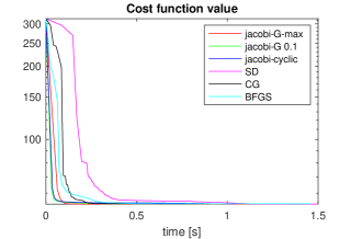
Figure 1: Cost function value (left) and norm of the gradient (right), Example 1

We do not expect this example to be easy for all of methods: this example is far from a diagonalizable, and we are not likely to be in a small neighborhood of a local extremum. We see that the Jacobi-type methods converge very fast, and for the versions of Algorithm 1 the gradient seems to converge to zero. We also see that the Jacobi-G-max version is the best compared to Jacobi-G with cyclic order and fixed $\delta$ (we tried different values of $\delta$).

We also consider a nearly diagonalizable case, $n=L=20$. We take $\boldsymbol{A}^{(\ell)}=\boldsymbol{Q}^{{\sf H}}\boldsymbol{D}^{(\ell)}\boldsymbol{Q}+\boldsymbol{E}^{(\ell)}$, where $\boldsymbol{Q}$ is a random unitary matrix, elements of $\boldsymbol{E}^{(\ell)}$ are i.i.d. realizations of Gaussian random variable with standard deviation $10^{-6}$, and $\boldsymbol{D}^{(\ell)}$ is a diagonal matrix, whose diagonal elements are equal to $1$, except the element ${D}^{(\ell)}_{\ell,\ell}=2$ (note that such matrices, without noise, satisfy Proposition 7.11).

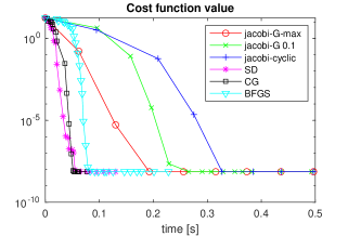
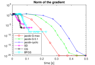
Figure 2: Cost function value (left) and norm of the gradient (right), Example 2

We plot the results in Figure 2. We see that the convergence of general-purpose Riemannian algorithms is much better in this case. Still, Jacobi algorithms converge in a few sweeps.

Note that in the current implementation (used to produce Figure 1 and Figure 2), we do not use the $O(Ln)$ update of $\boldsymbol{\Lambda}(\boldsymbol{U})$ as suggested in Section 8.1 (i.e., the matrix $\boldsymbol{\Lambda}(\boldsymbol{U})$ is recalculated at each step). This can be observed in Figure 2, where each marker for the Jacobi-type methods corresponds to one sweep. Thus, a further speedup of Jacobi-type methods is possible.

9 Discussion

In this paper, we showed that for a class of optimization problems on the unitary group (corresponding to approximate matrix and tensor diagonalization), convergence of Jacobi-type algorithms to stationary points can be proved (together with convergence rates). A gradient-based order of Givens rotations is adopted (which extends the approach of [32] for the real-valued case). By using the tools based on Łojasiewicz gradient inequality, we can ensure single-point convergence, under regularity conditions on one of the accumulation points; the speed of convergence is linear for the non-degenerate case, and local convergence can be proved. We also provided a characterization of Jacobi rotations for tensors of arbitrary orders.

Still, we believe that stronger results can be obtained. For the matrix case, although the Jacobi-type algorithms are similar in spirit to block-coordinate descent, they enjoy quadratic convergence (of the cost function value) for the classic matrix case [24] and the case of a pair of commuting matrices [13].

Also, in the matrix case, many results are available for cyclic strategies (at least weak convergence is known, see [24]). It would be interesting to see if similar results can be proved for tensor and joint matrix diagonalization cases; in fact, the convergence for the pure cyclic strategy is often observed in practice (see [38] for a comparison in the case of orthogonal group), but there is no convergence proof.

Note that we were not able to prove global single-point convergence, as in [38] (proved for 3rd order tensors or matrices). It seems that in the complex case, not only the order of rotations matters (which makes it similar to the higher-order case [38]). One possible track is to modify of a way to find the Jacobi rotation itself (i.e. adopt proximal-like steps if needed, see also [38]).

Another interesting question is whether we can relax the definition of single-point convergence. Indeed, if the critical point is degenerate (even in the quotient manifold), then a natural question is whether the potentially different accumulation points, belong the same critical manifold. This is, in fact, what is typically proved for the matrix case [20]: if there are multiple eigenvalues, then the convergence of invariant subspaces is guaranteed (which corresponds to the same critical manifold).

Appendix A Multilinear algebra proofs

Proof A.1 (Proof of Lemma 4.14).

The “only if” part follows from the fact that if $\boldsymbol{\mathcal{B}}$ is Hermitian, there exist tensors $\boldsymbol{\mathcal{A}}^{(1)},\ldots,\boldsymbol{\mathcal{A}}^{(L)}$ of order $d$ and real numbers $\alpha_{\ell}$, such that

(60) $$\boldsymbol{\mathcal{B}}=\sum\limits_{\ell=1}^{L}\alpha_{\ell}(\boldsymbol{\mathcal{A}}^{(\ell)})^{*}\otimes\boldsymbol{\mathcal{A}}^{(\ell)},\text{ i.e. }\mathcal{B}_{i_{1}\ldots i_{d}j_{1}\ldots j_{d}}=\sum\limits_{\ell=1}^{L}\alpha_{\ell}(\mathcal{A}^{(\ell)}_{i_{1}\ldots i_{d}})^{*}\mathcal{A}^{(\ell)}_{j_{1}\ldots j_{d}}.$$

This is nothing but the spectral theorem for Hermitian matrices applied to a matricization of $\boldsymbol{\mathcal{B}}$, see also [33, Propositions 3.5 and 3.9]. Then (60) implies that

$$g_{\boldsymbol{\mathcal{B}},d}(\boldsymbol{u})=\sum\limits_{\ell=1}^{L}\alpha_{\ell}|g_{\boldsymbol{\mathcal{A}}^{(\ell)},0}(\boldsymbol{u})|^{2}.$$

In order to prove the “if” part, we make the following remarks.

1. When restricted to $\|\boldsymbol{u}\|=1$, the order of the form can be always increased; Indeed, suppose that $\boldsymbol{\mathcal{T}}$ is $2(d-1)$-order Hermitian, then for all $\|\boldsymbol{u}\|=1$

   $$g_{\boldsymbol{\mathcal{T}},d-1}(\boldsymbol{u})=(\boldsymbol{\mathcal{T}}\otimes\boldsymbol{I}_{n})\mathop{\bullet_{1}}\boldsymbol{u}^{*}\cdots\mathop{\bullet_{d-1}}\boldsymbol{u}^{*}\mathop{\bullet_{d}}\boldsymbol{u}\cdots\mathop{\bullet_{2(d-1)}}\boldsymbol{u}\mathop{\bullet_{2d-1}}\boldsymbol{u}^{*}\mathop{\bullet_{2d}}\boldsymbol{u},$$

   where $\boldsymbol{I}_{n}$ is the identity; the expression on the right-hand side is a Hermitian form (39), where the $2d$-order tensor $\boldsymbol{\mathcal{B}}$ can be defined by permuting the indices:

   $$\mathcal{B}_{i_{1}\ldots i_{d}j_{1}\ldots j_{d}}=(\boldsymbol{\mathcal{T}}\otimes\boldsymbol{I}_{n})_{i_{1}\ldots i_{d-1}j_{1}\ldots j_{d-1}i_{d}j_{d}}=\mathcal{T}_{i_{1}\ldots i_{d-1}j_{1}\ldots j_{d-1}}(\boldsymbol{I}_{n})_{i_{d}j_{d}}.$$

2. Note that for any $t$, the function $|g_{\boldsymbol{\mathcal{A}},t}(\boldsymbol{u})|^{2}=g_{\boldsymbol{\mathcal{A}},t}(\boldsymbol{u})g^{*}_{\boldsymbol{\mathcal{A}},t}(\boldsymbol{u})$ is also a $2d$-form:

   (61) $$|g_{\boldsymbol{\mathcal{A}},t}(\boldsymbol{u})|^{2}=(\boldsymbol{\mathcal{A}}\otimes\boldsymbol{\mathcal{A}}^{*})\mathop{\bullet_{1}}\boldsymbol{u}^{*}\cdots\mathop{\bullet_{t}}\boldsymbol{u}^{*}\mathop{\bullet_{t+1}}\boldsymbol{u}\cdots\mathop{\bullet_{d+t}}\boldsymbol{u}\mathop{\bullet_{d+t+1}}\boldsymbol{u}^{*}\cdots\mathop{\bullet_{2d}}\boldsymbol{u}^{*},$$

   which can be written as $g_{\boldsymbol{\mathcal{B}},d}(\boldsymbol{u})$ for a tensor $\boldsymbol{\mathcal{B}}$ obtained by permuting indices:

   $$\mathcal{B}_{i_{1}\ldots i_{d}j_{1}\ldots j_{d}}=(\boldsymbol{\mathcal{A}}\otimes\boldsymbol{\mathcal{A}}^{*})_{i_{1}\ldots i_{t}j_{t+1}\ldots j_{d}j_{1}\ldots j_{t}i_{t+1}\ldots i_{d}}=\mathcal{A}_{i_{1}\ldots i_{t}j_{t+1}\ldots j_{d}}\mathcal{A}^{*}_{j_{1}\ldots j_{t}i_{t+1}\ldots i_{d}}.$$

   Finally, sums of Hermitian tensors are Hermitian, which completes the proof.

Proof A.2 (Proof of Theorem 4.21).

Since the cost function has the form (37), we have

$$\widetilde{h}(c,s_{1},s_{2})=g_{\boldsymbol{\mathcal{T}},d}(\left[\begin{smallmatrix}c\\ s^{\ast}\end{smallmatrix}\right])+g_{\boldsymbol{\mathcal{T}},d}(\left[\begin{smallmatrix}-s\\ c\end{smallmatrix}\right])$$

Let us rewrite the first term using the double contraction:

$$g_{\boldsymbol{\mathcal{T}},d}(\left[\begin{smallmatrix}c\\ s^{\ast}\end{smallmatrix}\right]) =\boldsymbol{\mathcal{T}}\mathop{\bullet_{1,d+1}}\left(\begin{bmatrix}c\\ s^{*}\end{bmatrix}^{*}\begin{bmatrix}c&s^{*}\end{bmatrix}\right)\cdots\mathop{\bullet_{d,2d}}\left(\begin{bmatrix}c\\ s^{*}\end{bmatrix}^{*}\begin{bmatrix}c&s^{*}\end{bmatrix}\right)$$

(62) $$=\frac{1}{2^{d}}\boldsymbol{\mathcal{T}}\mathop{\bullet_{1,d+1}}(\boldsymbol{I}_{2}+\boldsymbol{R})\mathop{\bullet_{2,d+2}}(\boldsymbol{I}_{2}+\boldsymbol{R})\cdots\mathop{\bullet_{d,2d}}(\boldsymbol{I}_{2}+\boldsymbol{R}),$$

$$\text{where }\boldsymbol{R}\stackrel{{\scriptstyle\sf def}}{{=}}\begin{bmatrix}2c^{2}-1&2cs^{\ast}\\ 2cs&1-2c^{2}\end{bmatrix},\quad\text{so that }\begin{bmatrix}c\\ s^{*}\end{bmatrix}^{*}\begin{bmatrix}c&s^{*}\end{bmatrix}=\begin{bmatrix}c^{2}&cs^{\ast}\\ cs&|s|^{2}\end{bmatrix}=\frac{1}{2}(\boldsymbol{I}_{2}+\boldsymbol{R}).$$

Similarly, by noting that

$$\begin{bmatrix}-s\\ c\end{bmatrix}^{*}\begin{bmatrix}-s&c\end{bmatrix}=\begin{bmatrix}|s|^{2}&-cs^{*}\\ -cs&c^{2}\end{bmatrix}=\frac{1}{2}(\boldsymbol{I}_{2}-\boldsymbol{R}),$$

we can rewrite the second term

(63) $$g_{\boldsymbol{\mathcal{T}},d}(\left[\begin{smallmatrix}-s\\ c\end{smallmatrix}\right])=\frac{1}{2^{d}}\boldsymbol{\mathcal{T}}\mathop{\bullet_{1,d+1}}(\boldsymbol{I}_{2}-\boldsymbol{R})\mathop{\bullet_{2,d+2}}(\boldsymbol{I}_{2}-\boldsymbol{R})\cdots\mathop{\bullet_{d,2d}}(\boldsymbol{I}_{2}-\boldsymbol{R}).$$

When summing (62) and (63), we note that the odd powers of $\boldsymbol{R}$ cancel, and the even powers have positive signs; therefore, due to symmetries we get

$$\widetilde{h}(c,s_{1},s_{2})=\frac{1}{2^{d-1}}\sum\limits_{j=0}^{m}{d\choose{2j}}\boldsymbol{\mathcal{T}}\mathop{\bullet_{1,d+1}}\boldsymbol{R}\cdots\mathop{\bullet_{2j,d+2j}}\boldsymbol{R}\mathop{\bullet_{2j+1,d+2j+1}}\boldsymbol{I}_{2}\cdots\mathop{\bullet_{d,2d}}\boldsymbol{I}_{2},$$

where the binomial coefficient appears when we sum over all possible locations of $\boldsymbol{R}$.

Next, we remark that $\boldsymbol{R}$ can be expressed in the following orthogonal basis

(64) $$\boldsymbol{R}=r_{1}\left[\begin{smallmatrix}1&0\\ 0&-1\end{smallmatrix}\right]+r_{2}\left[\begin{smallmatrix}0&-1\\ -1&0\end{smallmatrix}\right]+r_{3}\left[\begin{smallmatrix}0&i\\ -i&0\end{smallmatrix}\right],$$

where $\boldsymbol{r}=\begin{bmatrix}r_{1}&r_{2}&r_{3}\end{bmatrix}^{{\sf T}}=\begin{bmatrix}2c^{2}-1&-2cs_{1}&-2cs_{2}\end{bmatrix}^{{\sf T}}$ is defined in (30). Then by the multilinearity of the contractions, we can rewrite the expression for $\widetilde{h}(c,s_{1},s_{2})$ as

$$\widetilde{h}(c,s_{1},s_{2})=\sum\limits_{j=0}^{m}\boldsymbol{\mathcal{F}}^{(j)}\mathop{\bullet_{1}}\boldsymbol{r}\cdots\mathop{\bullet_{2j}}\boldsymbol{r},$$

where each $\boldsymbol{\mathcal{F}}^{(j)}$ is a symmetric complex $2j$-order $3\times\cdots\times 3$ tensor, whose entries are obtained by contractions of $\boldsymbol{\mathcal{T}}$ with basis matrices in (64) or $\boldsymbol{I}_{2}$.

It is only left to show that all the elements in each of the tensors $\boldsymbol{\mathcal{F}}^{(j)}$ are real. This is indeed the case, because for a Hermitian tensor $\boldsymbol{\mathcal{T}}$ contraction with one of the basis matrices keeps it Hermitian:

$$(\boldsymbol{\mathcal{T}}\mathop{\bullet_{1,d+1}}\left[\begin{smallmatrix}0&i\\ -i&0\end{smallmatrix}\right])_{i_{2}\ldots i_{d},j_{2}\ldots j_{d}}=-i(\mathcal{T}_{2i_{2}\ldots i_{d},1j_{2}\ldots j_{d}}-\mathcal{T}_{1i_{2}\ldots i_{d},2j_{2}\ldots j_{d}})$$

$$=i(\mathcal{T}^{*}_{2j_{2}\ldots j_{d},1i_{2}\ldots i_{d}}-\mathcal{T}^{*}_{1j_{2}\ldots j_{d},2i_{2}\ldots i_{d}})=((\boldsymbol{\mathcal{T}}\mathop{\bullet_{1,d+1}}\left[\begin{smallmatrix}0&i\\ -i&0\end{smallmatrix}\right])_{j_{2}\ldots j_{d},i_{2}\ldots i_{d}})^{*},$$

and similarly for contractions with $\left[\begin{smallmatrix}1&0\\ 0&-1\end{smallmatrix}\right]$, $\left[\begin{smallmatrix}0&-1\\ -1&0\end{smallmatrix}\right]$ and $\boldsymbol{I}_{2}$.

Finally, we note that, since $\|\boldsymbol{r}\|=1$, all the tensors $\boldsymbol{\mathcal{F}}^{(j)}$ can be combined in one tensor $\boldsymbol{\mathcal{F}}$ of order $2m$, as in the proof of Lemma 4.14 (see part (a) of the proof).

References

• [1] T. E. Abrudan, J. Eriksson, and V. Koivunen, Steepest descent algorithms for optimization under unitary matrix constraint, IEEE Trans. on Signal Process., 56 (2008), pp. 1134–1147.
• [2] P. A. Absil, R. Mahony, and B. Andrews, Convergence of the iterates of descent methods for analytic cost functions, SIAM Journal on Optimization, 16 (2005), pp. 531–547.
• [3] P.-A. Absil, R. Mahony, and R. Sepulchre, Optimization Algorithms on Matrix Manifolds, Princeton University Press, Princeton, NJ, 2008.
• [4] P. A. Absil, R. Mahony, and J. Trumpf, An extrinsic look at the Riemannian Hessian, in Geometric Science of Information: First International Conference, GSI 2013, F. Nielsen and F. Barbaresco, eds., Paris, France, 2013, Springer; Berlin Heidelberg, pp. 361–368.
• [5] A. Anandkumar, R. Ge, D. Hsu, S. M. Kakade, and M. Telgarsky, Tensor decompositions for learning latent variable models, Journal of Machine Learning Research, 15 (2014), pp. 2773–2832.
• [6] H. Attouch, J. Bolte, and B. F. Svaiter, Convergence of descent methods for semi-algebraic and tame problems: proximal algorithms, forward–backward splitting, and regularized Gauss–Seidel methods, Mathematical Programming, 137 (2013), pp. 91–129.
• [7] A. Banyaga and D. E. Hurtubise, A proof of the Morse-Bott lemma, Expositiones Mathematicae, 22 (2004), pp. 365 – 373.
• [8] R. Bott, Nondegenerate critical manifolds, Annals of Mathematics, 60 (1954), pp. 248–261.
• [9] N. Boumal, P.-A. Absil, and C. Cartis, Global rates of convergence for nonconvex optimization on manifolds, IMA Journal of Numerical Analysis, 39 (2019), pp. 1–33.
• [10] N. Boumal, B. Mishra, P.-A. Absil, and R. Sepulchre, Manopt, a Matlab toolbox for optimization on manifolds, Journal of Machine Learning Research, 15 (2014), pp. 1455–1459, http://www.manopt.org.
• [11] S. Boyd and L. Vandenberghe, Convex optimization, Cambridge University Press, 2004.
• [12] D. Brandwood, A complex gradient operator and its application in adaptive array theory, IEE Proceedings H - Microwaves, Optics and Antennas, 130 (1983), pp. 11–16.
• [13] A. Bunse-Gerstner, R. Byers, and V. Mehrmann, Numerical methods for simultaneous diagonalization, SIAM J. Matr. Anal. and Appl., 14 (1993), pp. 927–949.
• [14] J.-F. Cardoso and A. Souloumiac, Blind beamforming for non-gaussian signals, IEE Proceedings F-Radar and Signal Processing, 140 (1993), pp. 362–370.
• [15] J.-F. Cardoso and A. Souloumiac, Jacobi angles for simultaneous diagonalization, SIAM journal on matrix analysis and applications, 17 (1996), pp. 161–164.
• [16] P. Comon, From source separation to blind equalization, contrast-based approaches, in Int. Conf. on Image and Signal Processing (ICISP’01), Agadir, Morocco, May 2001, pp. 20–32. preprint: hal-01825729.
• [17] P. Comon, Contrasts, independent component analysis, and blind deconvolution, Int. J. Adapt. Control Sig. Proc., 18 (2004), pp. 225–243. preprint: hal-00542916.
• [18] P. Comon and C. Jutten, Handbook of Blind Source Separation: Independent component analysis and applications, Academic press, 2010.
• [19] L. De Lathauwer, Signal processing based on multilinear algebra, Katholieke Universiteit Leuven Leuven, 1997.
• [20] Z. Drmač, A global convergence proof for cyclic Jacobi methods with block rotations, SIAM J Matr. Anal. Appl., 31 (2010), pp. 1329–1350.
• [21] A. Edelman, T. A. Arias, and S. T. Smith, The geometry of algorithms with orthogonality constraints, SIAM journal on Matrix Analysis and Applications, 20 (1998), pp. 303–353.
• [22] B. Emile, P. Comon, and J. Le Roux, Estimation of time delays with fewer sensors than sources, IEEE Transactions on Signal Processing, 46 (1998), pp. 2012–2015.
• [23] P. M. N. Feehan, Optimal Łojasiewicz-Simon inequalities and Morse-Bott Yang-Mills energy functions, tech. report, 2018. arxiv:1706.09349.
• [24] G. Golub and C. Van Loan, Matrix Computations, JHU Press, 3rd ed., 1996.
• [25] B. Hall, Lie groups, Lie algebras, and representations: an elementary introduction, vol. 222, Springer, 2015.
• [26] V. Hari and E. B. Kovac, Convergence of the cyclic and quasi-cyclic block Jacobi methods, Electron. Trans. Numer. Anal, 46 (2017), pp. 107–147.
• [27] V. Hari and E. B. Kovač, On the convergence of complex Jacobi methods, Linear and Multilinear Algebra, (2019), pp. 1–26.
• [28] S. Helgason, Differential Geometry, Lie Groups, and Symmetric Spaces, Academic Press, 1978.
• [29] U. Helmke and J. B. Moore, Optimization and Dynamical Systems, Springer, 1994.
• [30] A. Hjørungnes and D. Gesbert, Complex-valued matrix differentiation: Techniques and key results, IEEE Transactions on Signal Processing, 55 (2007), pp. 2740–2746.
• [31] S. Hu and G. Li, Convergence rate analysis for the higher order power method in best rank one approximations of tensors, Numerische Mathematik, 140 (2018), pp. 993–1031.
• [32] M. Ishteva, P.-A. Absil, and P. Van Dooren, Jacobi algorithm for the best low multilinear rank approximation of symmetric tensors, SIAM J. Matrix Anal. Appl., 2 (2013), pp. 651–672.
• [33] B. Jiang, Z. Li, and S. Zhang, Characterizing real-valued multivariate complex polynomials and their symmetric tensor representations, SIAM J. Matr. Anal. and Appl., 37 (2016), pp. 381–408.
• [34] M. Kleinsteuber, U. Helmke, and K. Huper, Jacobi’s algorithm on compact Lie algebras, SIAM Journal on Matrix Analysis and Applications, 26 (2004), pp. 42–69.
• [35] S. Krantz and H. Parks, A Primer of Real Analytic Functions, Birkhäuser, Boston, 2002.
• [36] S. G. Krantz, Function theory of several complex variables, vol. 340, American Mathematical Soc., 2001.
• [37] C. Lageman, Convergence of gradient-like dynamical systems and optimization algorithms, doctoralthesis, Universität Würzburg, 2007.
• [38] J. Li, K. Usevich, and P. Comon, Globally convergent Jacobi-type algorithms for simultaneous orthogonal symmetric tensor diagonalization, SIAM J. Matr. Anal. Appl., 39 (2018), pp. 1–22.
• [39] S. Łojasiewicz, Une propriété topologique des sous ensembles analytiques réels, in Colloques internationaux du C.N.R.S, 117. Les Équations aux Dérivées Partielles, 1963, pp. 87–89.
• [40] W. F. Mascarenhas, On the convergence of the Jacobi method for arbitrary orderings, SIAM Journal on Matrix Analysis and Applications, 16 (1995), pp. 1197–1209.
• [41] E. Massart and P.-A. Absil, Quotient geometry with simple geodesics for the manifold of fixed-rank positive-semidefinite matrices, SIAM J. on Matr. Anal. and Appl., 41 (2020), pp. 171–198.
• [42] P. Mccullagh, Tensor Methods in Statistics, Monographs on Statistics and Applied Probability, Chapman and Hall, 1987.
• [43] J. Milnor, Morse theory, Princeton University Press, 1963.
• [44] J. Nie and Z. Yang, Hermitian tensor decompositions, (2019), https://arxiv.org/abs/1912.07175.
• [45] B. T. Polyak, Gradient methods for minimizing functionals, Zh. Vychisl. Mat. Mat. Fiz., 3 (1963), pp. 643–653.
• [46] T. Rapcsák, Geodesic convexity in nonlinear optimization, Journal of Optimization Theory and Applications, 69 (1991).
• [47] R. Schneider and A. Uschmajew, Convergence results for projected line-search methods on varieties of low-rank matrices via lojasiewicz inequality, SIAM J. Opt., 25 (2015), pp. 622–646.
• [48] A. Uschmajew, A new convergence proof for the higher-order power method and generalizations, Pac. J. Optim., 11 (2015), pp. 309–321.