Learning Temporal Causal Sequence Relationships
from Real-Time Time-Series

Abstract

We aim to mine temporal causal sequences that explain observed events (consequents) in time-series traces. Causal explanations of key events in a time-series have applications in design debugging, anomaly detection, planning, root-cause analysis and many more. We make use of decision trees and interval arithmetic to mine sequences that explain defining events in the time-series. We propose modified decision tree construction metrics to handle the non-determinism introduced by the temporal dimension. The mined sequences are expressed in a readable temporal logic language that is easy to interpret. The application of the proposed methodology is illustrated through various examples.

1 Introduction

This article presents an approach for learning causal sequence relationships, in the form of temporal properties, from data. Most realistic causal relationships are timed sequences of events that affect the truth of a target event. For example: “A car crashes into another. The cause was that there was a time-point 7 sec to 8 sec before the crash at which the two cars had a relative velocity of 70 kmph and a longitudinal distance of 6 m, and the leading car braked sharply.” In this relationship, the cause is the relative velocity, the distance between the cars, and the braking of the lead car. Such timing relationships can be expressed in logic languages such as Linear Temporal Logic (?) for discrete event systems and Signal Temporal Logic (?) for continuous and hybrid systems. Temporal logic properties are also extensively used in the semiconductor industry, with language standards such as SystemVerilog Assertions (SVA) (?) and Property Specification Language (PSL) (?). The notion of sequence expressions in SVA, which is very natural for expressing temporal sequences of events, is one of the primary features responsible for the popularity of the language in industrial practice. In this article we use a logic language inspired from SVA, which allows us to express real-valued timing relations between predicates. Our choice is partially influenced by our objective of mining assertions from circuit simulation traces, but also due to the applicability of the semantics of sequence expressions in other time-series domains. For instance, in our language, the causal expression for a crash may be captured as:

rspeed >= 70 && brake && ld <= 6 |-> ##[7:8] crash

In this expression, brake is a proposition, ld and rspeed are real-valued variables representing the longitudinal distance and relative velocity respectively, and rspeed>=70 and ld<=6 are predicates over real variables (PORVs).

Methods for learning causal relationships from data have been studied extensively and its importance is well established (?, ?, ?, ?, ?, ?). Most recently, the case was made for the need to build a framework for learning causal relationships using logic languages, to have explanations for predictions or recommendations and to understand cause-effect patterns from data, the latter being a necessary ingredient for achieving human level cognition (?). Causal learning has applications in many areas (?) including medical sciences, economics, education, environmental health and epidemiology. We aim to learn causal relationships as temporal properties, of the form $\alpha\Rightarrow\beta$, having a defined syntax and semantics. $\alpha$ is a sequence of Boolean expressions, with adjacent expressions separated from one another by time intervals. $\beta$ is a predicate whose cause is to be learned. Properties of this nature can be used for deduction. This then enables us to learn complex hierarchical causal relationships.

Existing learning approaches, such as neural networks, require large amounts of training data, and their results are not easily explainable. Furthermore, it is difficult to generalize the same network structure to a variety of domains. Alternately, using Bayes networks to capture causal relationships, poses ambiguities which are challenging to deal with when reasoning over time. Bayes networks do not explicitly indicate what events cause what; a variety of networks can be constructed for the same data. Also, time, which is a factor in our learning, introduces a natural partial order among the events. Furthermore, the data is a time-series representing the continuous evolution of variables over real-time, and therefore in our setting time is assumed to be dense by default, and the variables over which the predicates are defined are assumed to be continuous in general.

In this article, we use decision trees to achieve our goal of learning causal relationships. Traditional decision tree structures, as they exist in standard texts (?, ?, ?), deal with enumerated value domains of the variables. Continuous domains can be partitioned into a finite set of options by using predicates. For example, we may have the predicates, speed<30, 30<=speed<=100, and speed>100, to define low_speed, moderate_speed, and high_speed. In the temporal setting, speed, varies with time and hence the truths of these predicates change with time. When learning causal sequences which connect events in multiple time-worlds, the following fundamental challenges arise:

• A data-point is the state of a single time-world. For a time-series over real-time, in theory, there are infinite time-worlds in a finite time window.

• The influence of a predicate on the truth of the consequent changes with the time separation between them. In other words, the same predicate may contribute to the consequent being true in some time-worlds and false in some other time-worlds. Relative to the consequent, it means that different past time-worlds contribute to its truth in potentially conflicting ways.

• The influence of a time-world state on a future event (namely, the consequent) not only depends on the truth of the predicates in that time-world, but also on the truth of the predicates in past time-worlds.

The main challenges may therefore be summarized in terms of two questions, namely:

1. Finding the predicates which influence the consequent, and

2. For these predicates, finding the time window separating the predicates and the consequent, such that the sequence of predicates guarantee the consequent.

The challenges above arise due to the non-deterministic characteristic of temporal properties such as the one described earlier. In a temporal property, past time-worlds influence future time-worlds, and due to the dense nature of the real-time domain, these time-world associations are not always an exact association, and non-determinism in time plays a crucial role in representing these relationships.

Figure 1: Evidence of time-separations between events in different time-worlds.

In Fig. 1, various temporal associations are described. In Fig. 1(a), in one instance, event $e_{1}$ is separated from event $e_{2}$ by $t_{1}$ time units, and in another by $t^{\prime}_{1}$ time units. The system from which the traces have been taken may potentially admit infinite variations of time separation between $e_{1}$ and $e_{2}$ within a dense time interval. For learning meaningful associations we need to generalize from the discrete time separation instances shown in the time-series to time intervals. Fig. 1(b) depicts a similar situation with three events, where the separation between $e_{1}$ and $e_{2}$ can vary, and the separation between $e_{2}$ and event $e_{3}$ may also vary. Fig. 1(c) generalizes this.

The primary contributions of this article are as follows:

• We discuss the problems associated with using the standard decision tree learning framework for learning causal sequence relationships across multiple time-worlds. We show how this is attributed to the metrics used in building the decision tree.

• We adapt the measures of entropy, to account for time-worlds that may non-deterministically be classified into multiple classes.

• We also adapt the information gain metric to account for time-world states that may be present across multiple sibling nodes in the decision tree.

• We propose a logic language for representing causal sequences. The semantics of the language are compatible with standard ranking measures for assessing learned properties. We use measures of support and correlation to measure the quality of the learned properties. These measures also give insights into the data.

• We propose a decision tree construction that uses the adapted metrics to learn causal sequences across multiple time-worlds. We provide a method to translate the associations learned into properties, in a logic language that can be then used for reasoning.

The theory developed in this article has been implemented in a tool called the Prefix Sequence Inference Miner (PSI-Miner), available at https://github.com/antoniobruto/PSIMiner. The article is organized as follows. Section 2 outlines the problem statement with a motivating example and presents the formal language for representing the properties mined. Section 3 presents definitions for various structures and metrics used throughout this article. In Section 4, we extend the standard decision tree metrics to incorporate time into the learning process and develop an algorithm for mining temporal sequence expressions to derive explanations for a given target event. Section 5 introduces ranking metrics for properties. Section 6 discusses measures employed to prevent over-fitting using various stopping conditions and pruning methods. Section 7 describes how we extend structures and metrics to operate over multiple time-series simultaneously. In Section 8 we demonstrate the utility of the methodology through select case studies. Section 9 discusses related work. Section 10 concludes and summarizes the article.

2 Mining Explanation as Prefix Sequences

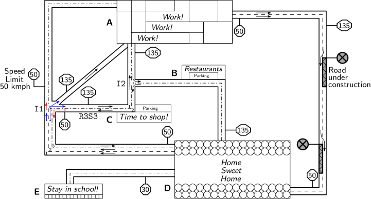
Figure 2: Vehicle road-map: Routes with demarcations for direction and speed limits.

We start with a motivating example. Figure 2 shows a map of town X, depicting roadways for vehicular movement in two dimensions. Vehicles are tagged with GPS devices to monitor their movements. The data contains patterns describing routes vehicles follow and their speed. Congestion and delays are reported in various parts of the town and one wishes to determine the causes that lead to a delay in reaching the office.

We label those states as delayed from which the delay in reaching office is inevitable. Obviously, the cause for a delay is a sequence of movement events that lead to a delayed state. Once in a delayed state, the vehicle is always delayed. Some events may be common to all vehicles reaching the office, and such events need to be separated out from those that contribute to the delay. Also, since the traffic pattern evolves with the time of the day, the time delays separating the relevant events have a significant role in capturing the causal sequence responsible for the delay.

Mining causes from the data leads to the discovery of the potential sequence of events leading to a delay. One such event sequence is as follows:

I1 ##[0:40] !LANE2 ##[0:5] !LANE1 && R3S3 |-> ##[0:30] DELAY

The formula reads as, “After being at Intersection-1 (I1), if the vehicle is not in Lane-2 (!LANE2) within the next 40 minutes, and is on road segment R3S3 but not in Lane-1 (!LANE1) within the next 5 minutes, then within the next 30 minutes, the vehicle is delayed.” On further examination, using the layout of roads, the town discovers that the vehicle was on the wrong lane while making the turn into R3S3 and ended up in the wrong lane in a high-speed zone. We call the language for describing the above property as the Prefix Sequence Inferencing language (PSI-L).

A prefix sequence inference (alternatively, a PSI-L formula or PSI-L property) has the general syntax, $\mathcal{S}$|->$E$; where, $\mathcal{S}$ is a prefix sequence of the form $s_{n}~{}\tau_{n}~{}s_{n-1}~{}\tau_{n-1}$ $\ldots\tau_{1}~{}s_{0}$, also known as a sequence expression.

A time interval $\tau_{i}$ is of the form $[a:b]$, $a,b\in\mathbb{R}^{\geq 0}$, $a\leq b$, and each $s_{i}$ is a Boolean expression of predicates. The length of the sequence expression is $n$ (having at most $n$ time intervals). A special case arises when $s_{0}=$ true and $\tau_{1}\neq\emptyset$. In such a case the prefix sequence inference is treated as the expression $s_{n}~{}\tau_{n}~{}s_{n-1}~{}\tau_{n-1}$ $\ldots\tau_{2}~{}s_{1}~{}$|->$~{}\tau_{1}~{}E$.

The consequent $E$ in a PSI-L formula is assumed to be given. It is in the context of $E$ that the antecedent $\mathcal{S}$ is learned. $E$ is called the target of the PSI-L formula. The notation $\mathcal{S}_{i}^{j}$ is used to denote the expression $s_{j}~{}\tau_{j}\ldots\tau_{i+1}~{}s_{i}$, $0\leq i\leq j\leq n$. In general, $\mathcal{S}\equiv\mathcal{S}_{0}^{n}$.

For variable set $V$, the set $\mathbb{D}=\mathbb{R}^{\geq 0}\times\mathbb{R}^{|V|}$ is the domain of valuations of timestamps and variables in $V$. A data point is a tuple $(t,\eta)\in\mathbb{D}$, $t\in\mathbb{R}^{\geq 0}$ and $\eta\in\mathbb{R}^{|V|}$. The value of a variable $x\in V$ at the data point $(t,\eta)$ is denoted by $\eta[x]$. Boolean and real-valued variables are treated in the same way in the implementation. A Boolean value at a data point is either 1 for true or 0 for false, and {$0,1$} $\subset\mathbb{R}$. We use the notation $\eta\models s$ to denote satisfaction of a Boolean expression $s$ by a valuation $\eta$ at a data point.

Definition 1.

Time-Series (Trace): A trace $\mathcal{T}$ is a finite ordered list of tuples $(t_{1},\eta_{1})$, $(t_{2},\eta_{2})$, $(t_{3},\eta_{3})\ldots(t_{d},\eta_{d})$, $\forall_{i\in\mathbb{N}_{d-1}}t_{i}<t_{i+1}$. The length of $\mathcal{T}$, the number of tuples in $\mathcal{T}$, expressed as $|\mathcal{T}|$, is $d$. The temporal length of $\mathcal{T}$, denoted $||\mathcal{T}||$, is $t_{d}-t_{1}$.

$\mathcal{T}(i)$, $i\in\mathbb{Z}^{>0}$ denotes the $i^{th}$ data point $(t_{i},\eta_{i})$ in trace $\mathcal{T}$.

A sub-trace $\mathcal{T}_{i}^{j}$ of $~{}\mathcal{T}$ is defined as the ordered list $(t_{i},\eta_{i})$, $(t_{i+1},\eta_{i+1})$, $\ldots(t_{j},\eta_{j})$; $i,j\in\mathbb{N}_{d}$ and $i\leq j$. ∎

Definition 2.

Match of a Sequence Expression and a PSI-L formula: The sequence expression $S_{l}^{m}::=s_{m}~{}\tau_{m}$ $s_{m-1}~{}\tau_{m-1}$ $\ldots\tau_{l+1}~{}s_{l}$ has a match at $\mathcal{T}(j)$ in sub-trace $\mathcal{T}_{i}^{j}$ of trace $\mathcal{T}$, denoted $\mathcal{T}_{i}^{j}{\models}S_{l}^{m}$ iff:

• $\eta_{i}\models s_{m}$, $\eta_{j}\models s_{l}$

• $\exists_{i\leq k\leq j}~{}\mathcal{T}_{k}^{j}\models S_{l}^{m-1}$ $\bigwedge$ $t_{k}-t_{i}\in\tau_{m}$ if $(m-1)>l$

A PSI-L formula can have multiple matches in $\mathcal{T}$. The PSI formula $S$|->$E$ has a match in trace $\mathcal{T}$ at $\mathcal{T}(j)$ iff $\exists_{1\leq i\leq j}$ $\mathcal{T}_{i}^{j}\models S$ and $\eta_{j}\models E$. ∎

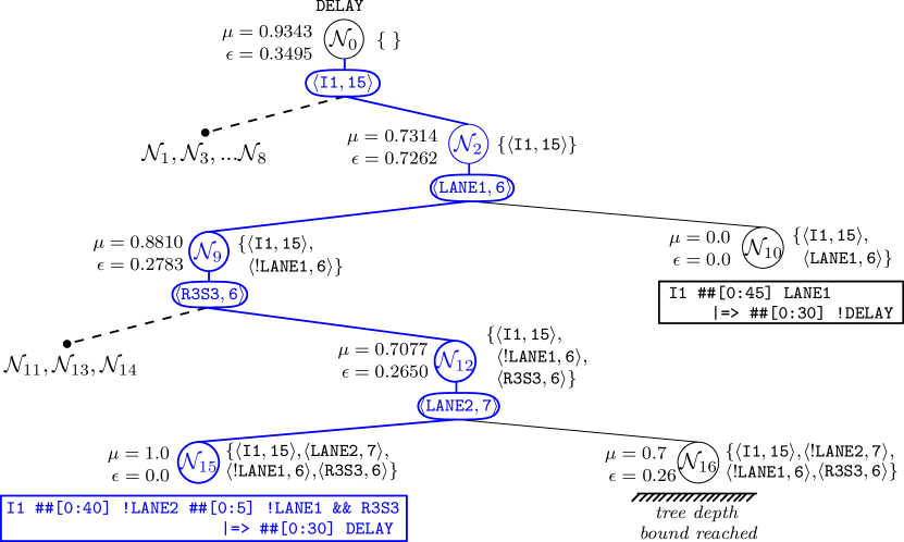
Figure 3: Decision Tree for mining causes of the delayed state DELAY for Town-X. A node is represented as a circle, a decision of the form $\langle predicate,bucket\rangle$ is an oval, decisions constraining a node are indicated to the right of each node within braces, while metrics for the node are on its right.

We consider a given predicate alphabet $\mathbb{P}$ and a predicate, $E\in\mathbb{P}$, that needs explanation, called the target. Given a finite set of traces $\mathbb{T}$ and a target $E$, we wish to find various prefix sequences that causally determine the truth of the target $E$. Each such prefix sequence produces a PSI-L formula, which is valid over all traces in $\mathbb{T}$.

We assume a bound $n\in\mathbb{N}$, $n\geq 0$, on the length of the prefix. We also use a parameter, $k\in\mathbb{R}^{\geq 0}$, called delay resolution, representing an initial upper bound on the time separating adjacent predicates in the prefix sequence. It is assumed that initially every time interval in the prefix sequence, $\tau_{i}=[0:k]$, $0\leq i\leq n$. The time intervals are refined as the PSI-L property is learned.

Before developing the theory behind mining PSI-L properties, we convey a high level intuitive outline of the approach, which we believe will help in the understanding of the notations and definitions that follow.

Given the target, $E$ (namely, the consequent), and the values of $n$ and $k$, we create a template of the following form:

$\sqcup_{n}$ ##[0:k] $\sqcup_{n-1}$ ##[0:k] $\ldots$ ##[0:k] $\sqcup_{1}$ ##[0:k] $\sqcup_{0}$ |-> E

where each $\sqcup_{i}$ is called a bucket and represents a placeholder for a Boolean combination of predicates (denoted $s_{i}$) from $\mathbb{P}$. Initially, therefore, given values for $n$ and $k$, the template describes a sequence of events spread over a time span of, at most, $n\times k$ time units before $E$. Our algorithm uses decision trees and works on this template in two cohesive ways, namely:

1. It uses novel metrics based on information gain to choose the combinations of predicates that go into a bucket. Not all buckets may be populated at the end – the intervals preceding and succeeding empty buckets are merged.

2. The delay intervals between populated buckets are narrowed to optimize the influence of the sequence expression on the target.

We use metrics based on interval arithmetic to compute the influence of predicates on the target across time intervals. The arithmetic is elucidated by hypothetically moving the target backwards in time, so that information gain metrics can be computed on individual time worlds.

An example of a decision tree produced by our algorithm for the property described earlier for the delayed state is shown in Figure 3. The path in the decision tree leading to the node at which a property is found is indicated using bold blue lines. A node in the decision tree is named as $\mathcal{N}$ and given an index. When the error $\epsilon$ at a node is non-zero, a choice of predicate and bucket is made and two child nodes are generated. If the decision tree depth bound is reached, no more decisions can be made. Some nodes, such as $\mathcal{N}_{10}$ and $\mathcal{N}_{15}$ are nodes with zero error. For such nodes, a property can be constructed using predicates and bucket positions labeling the path from the node to the root. A predicate is false on the left branch and true on the right branch. For instance, the property described earlier is generated at $\mathcal{N}_{15}$, and consists of the buckets $\sqcup_{15}=\{{\tt I1}\}$, $\sqcup_{7}=\{{\tt LANE2}\}$ and $\sqcup_{6}=\{{\tt!LANE1,R3S3}\}$. A delay resolution of $5$ is used here. The delays between buckets is computed using this delay resolution and the bucket indexes. Refinement of delays may be possible in some instances, and we explore this later.

3 PSI-Arithmetic and Preliminary Definitions

A summary of the methodology for mining prefix sequences is depicted in Figure 4. Initially, an event $E$ (the consequent) is presented as the target. Prefix sequences that appear to cause $E$ are to be mined (these are the potential antecedents). The antecedent and the consequent together define the mined property. It is important to note that the non-existence of a counter-example in the data is a necessary but not sufficient condition for a property to be mined.

The truth intervals of a predicate in a trace define a Boolean trace. The given trace is initially replaced by the Boolean traces corresponding to the predicate alphabet $\mathbb{P}$.

We use interval arithmetic to represent and analyze truths of predicates over dense-time. We handle time arithmetically, instead of as a series of samples, making the methodology robust to variations in the mechanism used for sampling the data. This also allows us to parameterize time delays between sequenced events, and compute the trade-offs involved while varying the temporal positions of the events. All definitions are with respect to a single trace for ease of explanation, but the methodology easily extends to dealing with multiple traces, as discussed later in Section 7.

Definition 3.

Interval Set of a predicate $P$ for trace $\mathcal{T}$: The Interval Set of a predicate $P$ for trace $\mathcal{T}$, $\mathcal{I}_{\mathcal{T}}(P)$, is the set of all non-overlapping maximal time intervals, $[a,b);~{}a,b\in\mathbb{R}_{\geq 0};~{}a<b$, in $\mathcal{T}$ where $P$ is true. The interval $[t_{i}:t_{j})\in\mathcal{I}_{\mathcal{T}}(P)$ iff $\forall_{i\leq k<j}\mathcal{T}(k)\models P$. The length of the interval set $\mathcal{I}_{\mathcal{T}}(P)$, denoted $|\mathcal{I}_{\mathcal{T}}(P)|$ is defined as,$|\mathcal{I}_{\mathcal{T}}(P)|=\Sigma_{\forall I=[a,b)\in\mathcal{I}_{\mathcal{T}}(P)}(b-a)$ For an interval $I=[a,b)$, the left and right values of the interval are denoted $l(I)$ and $r(I)$, denoting $a$ and $b$ respectively. ∎

Figure 4: Prefix Sequence Property Mining Workflow

Definition 4.

Truth Set for trace $\mathcal{T}$ and Predicate Set $\mathbb{P}$: The Truth Set for $\mathbb{P}$ in trace $\mathcal{T}$, $\mathbb{I}_{\mathcal{T}}(\mathbb{P})$, is the set of all Interval Sets for the trace $\mathcal{T}$ of all predicates $P\in\mathbb{P}$. $\mathbb{I}_{\mathcal{T}}=\{\mathcal{I}_{\mathcal{T}}(P)|P\in\mathbb{P}\}$.∎

Essentially, the trace $\mathcal{T}$ is translated into a Truth Set, namely the set of all labeled interval sets for predicates in $\mathbb{P}$. The truth set acts a Booleanized abstraction of the trace $\mathcal{T}$ with respect to $\mathbb{P}$.

Recall the following template of the mined properties as outlined in the previous section:

$\sqcup_{n}$ ##[0:k] $\sqcup_{n-1}$ ##[0:k] $\ldots$ ##[0:k] $\sqcup_{1}$ ##[0:k] $\sqcup_{0}$ |-> E

where each $\sqcup_{i}$ is called a bucket. We propose a decision tree learning methodology for mining prefix sequences. Every path of the learned decision tree leads to a true or false decision, representing the truth of the consequent. Each node of the decision tree corresponds to a pair $\langle P,i\rangle$, namely a chosen predicate and its position (the bucket) in the prefix sequence. Different branches correspond to different choices of predicates in different buckets. The accumulated choices along a path of the decision tree define a partial prefix sequence, where some of the buckets have been populated. These accumulated choices shall be referred to as a constraint set.

Definition 5.

Constraint Set: A constraint is a pair, $\langle P,i\rangle$, consisting of a predicate, $P$, and its position in the prefix-sequence, where $P\in\mathbb{P}$, $i\in[0:n]$, $n\in\mathbb{N}$. A constraint set $\mathcal{C}$ is a set of constraints at a node in the decision tree obtained by accumulating the constraints at its ancestors in the tree. ∎

Definition 6.

Prefix-Bucket: For a constraint set $\mathcal{C}$, the prefix-bucket at position $i\in\mathbb{N}$, given as $\mathcal{B}_{i}(\mathcal{C})$, is the set of all predicates $P$, where $\langle P,i\rangle\in\mathcal{C}$. The set of all buckets for a constraint set $\mathcal{C}$ is written as $\mathbb{B}(\mathcal{C})$ or simply $\mathbb{B}$ if constraint set $\mathcal{C}$ is known from context.

The term prefix-bucket refers to the set of constraints in a bucket. When the constraint set $\mathcal{C}$ is known, we use the notation $\mathcal{B}_{i}$ to mean $\mathcal{B}_{i}(\mathcal{C})$.

The set of constraints in $\mathcal{C}$ define a partial prefix in PSI-L. In the prefix-sequence $s_{n}~{}\tau_{n}~{}s_{n-1}~{}\tau_{n-1}\ldots\tau_{1}~{}s_{0}$, the sub-expression $s_{i}$, $0\leq i\leq n$, is formed by the conjunction of predicates in the bucket $\mathcal{B}_{i}(\mathcal{C})$. The partial prefix sequence formed from the constraint set $\mathcal{C}$ is denoted as $\mathcal{S}_{\mathcal{C}}$. For a constraint set $\mathcal{C}$, the interval set for bucket $\mathcal{B}_{i}$, given as $\mathcal{I}_{\mathcal{T}}(\mathcal{B}_{i})$, is the set of truth intervals where the constraints in $\mathcal{B}_{i}$ are all true. ∎

The learning algorithm must place predicate and event constraints into various buckets. Some buckets may remain empty, resulting in the delays in the sequence that appear before and after it to merge.

Definition 7.

Interval Work-Set: An interval work-set $\mathcal{W}_{0}^{n}$ is a set, $\{{I}_{\mathcal{B}_{0}},I_{\mathcal{B}_{1}},{I}_{\mathcal{B}_{2}},...,{I}_{\mathcal{B}_{n}}|$ ${I}_{\mathcal{B}_{i}}\in\mathcal{I}_{\tau}(\mathcal{B}_{i}),0\leq i\leq n\}$, of labeled truth intervals for the set of labelled buckets, $\mathbb{B}=\{\mathcal{B}_{0}$, $\mathcal{B}_{1}$, $\mathcal{B}_{2}$,…, $\mathcal{B}_{n}\}$, of constraint set $\mathcal{C}$. We also define $\mathcal{W}_{i}^{k}=\{{I}_{\mathcal{B}_{j}}|i\leq j\leq k\}$.

For trace $\mathcal{T}$, different combinations of bucket truth intervals, produce unique interval work-sets. The set of all work sets that can be derived from $\mathcal{I}_{\tau}(\mathcal{B}_{i}),0\leq i\leq n$, is given as $\mathbb{W}_{\mathcal{C}}$ or simply $\mathbb{W}$ when the context $\mathcal{C}$ is known. ∎

Intuitively, each Interval Work-Set is constructed by choosing one interval from each prefix bucket. This has been further illustrated in Example 1.

We use the notion of Forward Influence to find the set of time points that qualify as a match for a prefix sequence following Definition 2. Since the designated time of the match is the time at which the match ends, we refer to these time points as end-match times. End-match times can be spread over an interval, and we shall refer to such intervals as end-match intervals.

Definition 8.

Forward Influence $\mathds{F}(\mathcal{S},\mathcal{W}_{0}^{n})$: The forward influence for a prefix sequence expression $\mathcal{S}=s_{n}~{}\tau_{n}~{}s_{n-1}~{}...~{}\tau_{1}~{}s_{0}$, given the interval work-set $\mathcal{W}_{0}^{n}=\{{I}_{\mathcal{B}_{0}},...,{I}_{\mathcal{B}_{n}}\}$, is an interval, recursively defined as follows:

$\mathds{F}(\mathcal{S},\mathcal{W}_{i}^{i})$	$=$	${I}_{\mathcal{B}_{i}}$
$\mathds{F}(\mathcal{S},\mathcal{W}_{i}^{j})$	$=$	$(\mathds{F}(\mathcal{S},\mathcal{W}_{i+1}^{j})\oplus\tau_{i})~{}\cap~{}{I}_{\mathcal{B}_{i}}$ , $0\leq i<j\leq n$

where, $\oplus$ represents the Minkowski sum of intervals: $[\alpha:\beta]\oplus[a:b]=[\alpha+a:\beta+b]$. For $\mathcal{S}$, the set of intervals in $\mathds{F}(\mathcal{S},\mathcal{W}_{0}^{n})$ are called the end-match intervals of $\mathcal{S}$. The set of all forward influence intervals over all work sets $\mathbb{W}$, is $\mathds{F}(\mathcal{S},\mathbb{W})=\bigcup_{\begin{subarray}{c}\mathcal{W}_{0}^{n}\in\mathbb{W}\end{subarray}}\mathds{F}(\mathcal{S},\mathcal{W}_{0}^{n})$. ∎

Example 1.

Consider the sequence expression $\mathcal{S}$ $\equiv$ $s_{2}$ ##[1:4] $s_{1}$ ##[2:8] $s_{0}$, and bucket truth interval sets for a trace $\mathcal{T}$, $\mathcal{I}_{\mathcal{T}}(\mathcal{B}_{2})=\{[2:4]\}$, $\mathcal{I}_{\mathcal{T}}(\mathcal{B}_{1})=\{[3:5],[7:9]\}$ and $\mathcal{I}_{\mathcal{T}}(\mathcal{B}_{0})=\{[4:9],[12:19]\}$. There are $1\times 2\times 2=4$ interval work-sets.

The computation of forward influence using Definition 8, for each possible interval work-set is described in the form of a tree in Figure 5(a). An interval work-set is the set of truth intervals of buckets encountered along a path from the root to a leaf node in the tree. The tree is rooted at a node corresponding to the truth interval $[2:4]$ for $\mathcal{B}_{2}$. Level $i$ in the tree corresponds to the computation of $\mathds{F}(\mathcal{S},\mathcal{W}_{i}^{2})$.

The sequence expression, therefore, has four end-match intervals, namely $[5:9]$, $[9:9]$, $[12:13]$, and $[12:16]$. These intervals are contributed by different combinations of truth intervals of the constituting predicates (that is, different interval work-sets), and may have overlaps. ∎

Even though a truth interval of a predicate in the work-set may contribute to a match of a sequence expression, not all the points in that truth interval may participate in the contribution. In other words, it is quite possible that only some sub-interval of a truth interval actually takes part in the forward influence. Finding such sub-intervals eventually leads us to find the begin-match intervals for a sequence expression.

In order to find the sub-intervals of the intervals in the work-set, we use a backward influence computation as defined below.

(a) Forward Influence computation

(b) Backward Influence computation

Figure 5: Influences computed for $\mathcal{B}_{2}\#\#[1:4]~{}\mathcal{B}_{1}\#\#[2:8]~{}\mathcal{B}_{0}$, with $\mathcal{I}_{\tau}(\mathcal{B}_{2})=\{[2:4]\}$, $\mathcal{I}_{\tau}(\mathcal{B}_{1})=\{[3:5],[7:9]\}$ and $\mathcal{I}_{\tau}(\mathcal{B}_{0})=\{[4:9],[12:19]\}$

Definition 9.

Backward Influence $\mathds{B}(\mathcal{S},\mathcal{W}_{0}^{n},i)$: The backward influence, $\mathds{B}(\mathcal{S},\mathcal{W}_{0}^{n},i)$, $i\in[0,n]$, for a sequence expression $S=s_{n}~{}\tau_{n}~{}s_{n-1}~{}...~{}\tau_{1}~{}s_{0}$, given the interval work-set $\mathcal{W}_{0}^{n}=\{{I}_{\mathcal{B}_{0}},{I}_{\mathcal{B}_{1}},...,{I}_{\mathcal{B}_{n}}\}$, is an interval defined as follows:

$\mathds{B}(\mathcal{S},\mathcal{W}_{0}^{n},0)$	$=$	$\mathds{F}(\mathcal{S},\mathcal{W}_{0}^{n})$
$\mathds{B}(\mathcal{S},\mathcal{W}_{0}^{n},i)$	$=$	$(\mathds{B}(\mathcal{S},\mathcal{W}_{0}^{n},i-1)\ominus\tau_{i})\cap\mathds{F}(\mathcal{S},\mathcal{W}_{i}^{n})$ , $0<i\leq n$

where, $\ominus$ represents the Minkowski difference of intervals: $[\alpha:\beta]\ominus[a:b]=[\alpha-b:\beta-a]$. For $\mathcal{S}$, the set of intervals in $\mathds{B}(\mathcal{S},\mathcal{W}_{0}^{n},n)$ are called the begin-match intervals of $\mathcal{S}$. The set of all backward influence intervals at position $i$, over all work sets $\mathbb{W}$, is $\mathds{B}(\mathcal{S},\mathbb{W},i)=\bigcup_{\begin{subarray}{c}\mathcal{W}_{0}^{n}\in\mathbb{W}\end{subarray}}\mathds{B}(\mathcal{S},\mathcal{W}_{0}^{n},i)$. ∎

For a given prefix sequence expression $\mathcal{S}$ having at most $n$ time intervals, and interval work-set $\mathcal{W}_{0}^{n}$, we use the shorthand notation $\mathds{F}_{0}^{i}$ to represent $\mathds{F}(\mathcal{S},\mathcal{W}_{0}^{i})$, and $\mathds{B}_{0}^{i}$ to represent $\mathds{B}(\mathcal{S},\mathcal{W}_{0}^{n},i)$. Computing backward influences will, as we see later, also allow us to refine delay intervals between non-empty buckets of a learned property.

Example 2.

We continue with the example of Figure 5(a). For each interval set, the backward influence is computed, using Definition 9. The computation begins with the leaves of the tree in Figure 5(a), and proceeds backwards through the sequence expression to determine the intervals corresponding to each match, indicated as a bottom-up computation in Figure 5(b).

In a sequence expression computing the forward influence is not sufficient to identify the sequence of intervals contributing to a match. We explain this using Figure 5(b). Observe the second column in Figure 5(b) corresponding to the interval work-set $\mathcal{W}_{0}^{2}=\{[12:19]_{\mathcal{B}_{0}},[3:5]_{\mathcal{B}_{1}},[2:4]_{\mathcal{B}_{2}}\}$. From Figure 5(a), the forward influence computes the influence intervals to be $[2:4]$, $[3:5]$, $[12:13]$. The interval $[3:5]$ corresponds to the forward influence match up to $\mathcal{B}_{1}$. The truth interval of $\mathcal{B}_{0}$ under consideration for this match is the interval $[12:19]$. Of the truth interval $[3:5]$ of $\mathcal{B}_{1}$, observe that $[3:4)\oplus[2:8]=[5:12)$, $[5:12)\cap[12:19]=\emptyset$, which does not fall within the truth interval $[12:19]$ of $\mathcal{B}_{0}$, and thus truth interval $[3:4)$ cannot contribute to a match. On the other hand, $[4:5]\oplus[2:8]=[6:13]$, and $[6:13]\cap[12:19]=[12:13]$. Therefore, of the interval $[3:5]$, only $[4:5]$ contributes to a match. ∎

Observation 1.

For a potential infinite continuum of prefix sequence expression matches associated with an interval work-set, the forward-influence computes the corresponding end-match time intervals, and the backward influence computes sub-intervals from work-sets that take part in matches. ∎

Recall, that we use the shorthand notation $\mathcal{S}_{\mathcal{C}}$ to represent the prefix sequence constructed from constraint-set $\mathcal{C}$.

Definition 10.

Influence Set The influence set for a sequence expression for constraint set $\mathcal{C}$, $S_{\mathcal{C}}=s_{n}~{}\tau_{n}~{}s_{n-1}~{}...~{}\tau_{1}~{}s_{0}$, given interval sets for each bucket, $\mathcal{I}_{\mathcal{T}}(\mathcal{B}_{i})$, $0\leq i\leq n$, is defined as the union of end-match intervals over all possible work sets $\mathcal{W}_{0}^{n}\in\mathbb{W}$, defined as follows: $\mathcal{I}_{\mathcal{T}}(\mathcal{S}_{\mathcal{C}})=\bigcup_{\begin{subarray}{c}\mathcal{W}_{0}^{n}\in\mathbb{W}\end{subarray}}\mathds{F}(\mathcal{S}_{\mathcal{C}},\mathcal{W}_{0}^{n})$ ∎

Definition 11.

Length of a Truth Set: The length of a Truth Set $\mathbb{I}_{\mathcal{T}_{\mathcal{C}}}(\mathbb{P})$, under constraint set $\mathcal{C}$, represented by $|\mathbb{I}_{\mathcal{T}_{\mathcal{C}}}(\mathbb{P})|$ is the length of the influence set, given as $|\mathcal{I}_{\mathcal{T}}(\mathcal{S}_{\mathcal{C}})|$. ∎

Example 3.

We continue with the example of Figure 5(a). The set of all possible work sets, $\mathbb{W}$, in the figure, is $\mathbb{W}=\{\{[4:9]_{\mathcal{B}_{0}},[3:5]_{\mathcal{B}_{1}},[2:4]_{\mathcal{B}_{2}}\},\{[4:9]_{\mathcal{B}_{0}},[7:9]_{\mathcal{B}_{1}},[2:4]_{\mathcal{B}_{2}}\},\{[12:19]_{\mathcal{B}_{0}},[3:5]_{\mathcal{B}_{1}},[2:4]_{\mathcal{B}_{2}}\},\{[12:19]_{\mathcal{B}_{0}},[7:9]_{\mathcal{B}_{1}},[2:4]_{\mathcal{B}_{2}}\}\}$. Let $\mathcal{C}$ be the constraint set forming the buckets in the sequence-expression. The influence set for $\mathcal{S}_{\mathcal{C}}$, is computed in Example 1 using forward influence. The influence set is $\mathcal{I}_{\mathcal{T}}(\mathcal{S}_{\mathcal{C}})=\{[5:9],[9:9],[12:13],[12:16]\}$. The length of the truth set for $\mathcal{S}_{\mathcal{C}}$ is $|\mathcal{I}_{\mathcal{T}}(\mathcal{S}_{\mathcal{C}})|=9-5+9-9+13-12+16-12=9$. ∎

This section may be summarized as follows. Properties over dense real-time may match over a continuum of time points. We use time intervals to represent truth points for predicates (Definition 3) and sets of predicates (Definition 4). A prefix sequence is built from a set predicate constraints (Definition 5), where each predicate occupies a fixed position (bucket) in the prefix sequence. Multiple predicates sharing the same position in the sequence form a prefix-bucket (Definition 6). A predicate can be true over multiple disjoint time intervals. All predicates in the same bucket are conjuncted together, and hence a bucket of predicates may be true over a set of intervals. Choosing a combination of truth intervals, one truth interval from each bucket position, forms an interval work-set (Definition 7). For the prefix-sequence and a given work-set, the forward influence (Definition 8) provides a mechanism for computing the end time-points associated with the match of the prefix-sequence , while the backward influence (Definition 9) provides a mechanism for computing the begin time-points associated with the matching end time-points of the forward influence. The set of all end time-points for all work-sets of a prefix-sequence form a set of intervals where the prefix-sequence has influence, the influence set (Definition 10). The choice of constraints $\mathcal{C}$ limits the length of the truth set (Definition 11), and determines the decisions made for mining additional constraints.

4 Learning Decision Trees for Sequence Expressions

This section develops the methodology for learning decision trees treating the target as the decision variable. Each path of the decision tree from the root to a leaf will represent a prefix sequence for the target or its negation.

The semantics of sequence expressions allow for both, immediate causality and future causality to be asserted. Immediate causality, expressed as $\mathcal{S}$ |-> $E$, is observed when the truth of sequence $\mathcal{S}$ at time $t$ causes the consequent $E$ to be true at time $t$. Future causality, expressed by the assertion $\mathcal{S}$ |-> ##[a:b] $E$ relates the truth of the sequence $\mathcal{S}$ at time $t$ with the truth of $E$ at time $t^{\prime}\in[t+a:t+b]$. In both these forms, $E$ is Boolean, and $\mathcal{S}$ is, by default, a temporal sequence expression.

An important special case of immediate causal relations consists of relations where $\mathcal{S}$ is strictly Boolean and does not contain any delay interval. We first present decision making metrics available in standard texts (?) that we have adapted to interval sets for mining immediate causal relations of this type. Later, we demonstrate through examples that these metrics can lead to incorrect decisions when $\mathcal{S}$ is temporal. At the end, we present metrics and a decision tree algorithm to learn sequence expressions to express future causality relations.

4.1 Decision Metrics for learning Immediate Relations

At each node of the decision tree, statistical measures of Mean and Error are used to evaluate the node. Standard decision tree algorithms use measures of Entropy or Ginni-Index (?) to measure the disorder and chaos in the data.

For immediate relations of the form $S$ |-> $E$, where $\mathcal{S}$ and $E$ are Boolean expressions, the property template is $\sqcup_{0}$ |-> E, and standard Shannon Entropy is used as a measure of disorder. Information gain is used to evaluate decisions at internal nodes of the decision tree.

Definition 12.

Mean${}_{\mathcal{T}_{\mathcal{C}}}$(E) (?): For the target $E$, the proportion of time in trace $\mathcal{T}$ that $E$ is true in the trace constrained by $\mathcal{C}$:

$$Mean_{\mathcal{T}_{\mathcal{C}}}(E)=\frac{|\mathcal{I}_{\mathcal{T}}(E)\cap\mathcal{I}(\mathcal{S}_{\mathcal{C}})|}{|\mathcal{I}(\mathcal{S}_{\mathcal{C}})|}$$

The mean represents the conditional probability of $E$ being true under the influence of the constraints in $\mathcal{C}$. For convenience, we use $\mu_{\mathcal{T}_{\mathcal{C}}}(E)$ to refer to $Mean_{\mathcal{T}_{\mathcal{C}}}(E)$. The mean is not defined when $|\mathcal{I}(\mathcal{S}_{\mathcal{C}})|=0$. ∎

Note that for this special case of immediate causality, the mean represents the conditional probability of $E$ being true under the immediate influence of the constraints in $\mathcal{C}$. Also, there is only one immediate bucket, $\sqcup_{0}$, and therefore all members of $\mathcal{C}$ correspond to the same bucket. This means $\mathcal{I}(\mathcal{S}_{\mathcal{C}})$ corresponds to those regions of the trace which satisfy all predicates in $\mathcal{C}$.

Lemma 1.

The mean, $\mu_{\mathcal{T}_{\mathcal{C}}}(E)$ is 1 if and only if $E$ is true wherever $\mathcal{S}_{\mathcal{C}}$ is true, and 0 if and only if $E$ is false wherever $\mathcal{S}_{\mathcal{C}}$ is true.

Proof.

If $E$ is true wherever $\mathcal{S}_{\mathcal{C}}$ is true, then $\mathcal{I}_{\mathcal{T}}(E)\cap\mathcal{I}(\mathcal{S}_{\mathcal{C}})=\mathcal{I}(\mathcal{S}_{\mathcal{C}})$, therefore $\mu_{\mathcal{T}_{\mathcal{C}}}(E)=1$. Conversely, if $\mu_{\mathcal{T}_{\mathcal{C}}}(E)=1$, then $|\mathcal{I}_{\mathcal{T}}(E)\cap\mathcal{I}(\mathcal{S}_{\mathcal{C}})|=|\mathcal{I}(\mathcal{S}_{\mathcal{C}})|$, which is possible only in the situation where $\mathcal{I}_{\mathcal{T}}(E)\cap\mathcal{I}(\mathcal{S}_{\mathcal{C}})=\mathcal{I}(\mathcal{S}_{\mathcal{C}})$. Similarly, it can be shown that E is false whenever $\mu_{\mathcal{T}_{\mathcal{C}}}(E)=0$. ∎

Definition 13.

Error${}_{\mathcal{T}_{\mathcal{C}}}(E)$(?): For the target class $E$, the error for the trace $\mathcal{T}$ constrained by $\mathcal{C}$ is defined as follows:

$$Error_{\mathcal{T}_{\mathcal{C}}}(E) =-\mu_{\mathcal{T}_{\mathcal{C}}}(E)\times log_{2}(\mu_{\mathcal{T}_{\mathcal{C}}}(E))-\mu_{\mathcal{T}_{\mathcal{C}}}(\neg E)\times log_{2}(\mu_{\mathcal{T}_{\mathcal{C}}}(\neg E))$$

For convenience, we use $\epsilon_{\mathcal{T}_{\mathcal{C}}}(E)$ to refer to $Error_{\mathcal{T}_{\mathcal{C}}}(E)$. ∎

Lemma 2.

For an immediate property, the error, $\epsilon_{\mathcal{T}_{\mathcal{C}}}$(E) for constraint set $\mathcal{C}$ and consequent $E$ is zero if and only if $\mathcal{S}_{\mathcal{C}}$ decides the truth of $E$ or $\neg E$, that is, either there are no counter-examples for $\mathcal{S}_{\mathcal{C}}$|->$E$ or there are no counter-examples for $\mathcal{S}_{\mathcal{C}}$|->$\neg E$.

Proof.

We assume that $|\mathcal{I}(\mathcal{S}_{\mathcal{C}})|>0$, the sum of lengths of truth intervals for the expression describing $\mathcal{C}$ is non-zero.

Part A: Consider the property $\mathcal{S}_{\mathcal{C}}$|->$E$, where $|\mathcal{I}_{\mathcal{T}}(E)\cap\mathcal{I}(\mathcal{S}_{\mathcal{C}})|>0$. Assume that there are counter-examples for $\mathcal{S}_{\mathcal{C}}$|->$E$. The counter-examples would introduce a non-zero time interval when $\mathcal{S}_{\mathcal{C}}$ is true and $E$ is false. Let one of the counter-example time-intervals be the interval $[a:b)$, where $b>a$. Therefore, $|\mathcal{I}_{\mathcal{T}}(\neg E)\cap\mathcal{I}(\mathcal{S}_{\mathcal{C}})|>0$, hence $\mu_{\mathcal{T}_{\mathcal{C}}}(\neg E)>0$, and $log_{2}(\mu_{\mathcal{T}_{\mathcal{C}}}(\neg E)))<0$ (the mean is bounded between 0 and 1). Similarly the term, $\mu_{\mathcal{T}_{\mathcal{C}}}(E)\times log_{2}(\mu_{\mathcal{T}_{\mathcal{C}}}(E)))<0$, since $|\mathcal{I}_{\mathcal{T}}(\neg E)\cap\mathcal{I}(\mathcal{S}_{\mathcal{C}})|>0$ . Hence, from Definition 13, $\epsilon_{\mathcal{T}_{\mathcal{C}}}(E)>0$.

Consider the property $\mathcal{S}_{\mathcal{C}}$|->$E$, where $|\mathcal{I}_{\mathcal{T}}(E)\cap\mathcal{I}(\mathcal{S}_{\mathcal{C}})|=|\mathcal{I}(\mathcal{S}_{\mathcal{C}})|$. Hence, $|\mathcal{I}_{\mathcal{T}}(\neg E)\cap\mathcal{I}(\mathcal{S}_{\mathcal{C}})|=0$. Hence $\mu_{\mathcal{T}_{\mathcal{C}}}(E)=1$, $\mu_{\mathcal{T}_{\mathcal{C}}}(\neg E)=0$ and hence $Error_{\mathcal{T}}(E)=0$.

The proof for when the property is of the form $\mathcal{S}_{\mathcal{C}}$|->$\neg E$ is identical.

Part B: Conversely, if the error is non-zero, then both terms of Definition 13 are non-zero (the intervals for $E$ and $\neg E$ are compliments of each other). From Definition 12, $\mu_{\mathcal{T}_{\mathcal{C}}}(E)>0$, $\mu_{\mathcal{T}_{\mathcal{C}}}(\neg E)>0$, and hence $\mathcal{I}_{\mathcal{T}}(E)\cap\mathcal{I}(\mathcal{S}_{\mathcal{C}})\neq\mathcal{I}(\mathcal{S}_{\mathcal{C}})$ and $\mathcal{I}_{\mathcal{T}}(\neg E)\cap\mathcal{I}(\mathcal{S}_{\mathcal{C}})\neq\mathcal{I}(\mathcal{S}_{\mathcal{C}})$. Therefore, there exists a non-empty interval $[a_{1}:b_{1})$, $b_{1}>a_{1}$ where $\mathcal{S}_{\mathcal{C}}$ is true and $E$ is false, and there exists a non-empty interval $[a_{2}:b_{2})$, $b_{2}>a_{2}$ where $\mathcal{S}_{\mathcal{C}}$ is true and $E$ is true, respectively representing counter-example intervals for $\mathcal{S}_{\mathcal{C}}$|->$E$ and $\mathcal{S}_{\mathcal{C}}$|->$\neg E$. ∎

We aim to construct a decision tree where the target, $E$, is the decision variable. Each node of the decision tree represents a predicate, which is chosen on the basis of its utility in separating the cases where $E$ is true from the cases where $E$ is false. Each branch out of a node represents one of the truth values of the predicate representing that node. The set of cases at an intermediate node of the decision tree are the time points at which the predicates from the root to that node have precisely the values representing the edges along that path (recall the definition of a constraint set).

This utility metric is called the gain. While many gain metrics exist (?), we find that Information Gain works best for our two class application. The standard definition of Information Gain is given below.

Definition 14.

Gain (?): The gain (improvement in error) of choosing $P\in\mathbb{P}$ to add to constraint set $\mathcal{C}$, at a node having error $\epsilon_{\mathcal{T}_{\mathcal{C}}}(E)$ is as follows:

$$Gain=\epsilon_{\mathcal{T}_{\mathcal{C}}}(E)-\frac{|\mathcal{I}(\mathcal{S}_{\mathcal{C}\cup\{P\}})|}{|\mathcal{I}(\mathcal{S}_{\mathcal{C}})|}\times\epsilon_{\mathcal{T}_{\mathcal{C}\cup\{P\}}}(E)-\frac{|\mathcal{I}(\mathcal{S}_{\mathcal{C}\cup\{\neg P\}})|}{|\mathcal{I}(\mathcal{S}_{\mathcal{C}})|}\times\epsilon_{\mathcal{T}_{\mathcal{C}\cup\{\neg P\}}}(E)\qed$$

Applying traditional decision tree learning using Definitions 13 and 14 on the truth-set is suitable for mining those immediate properties where the antecedent, $\mathcal{S}$, is Boolean.

To mine prefix sequences with delays, $E$’s truth must be tested with the truth of other predicates over past time points. In Section 4.2, we introduce the notion of pseudo-targets that allow us to evaluate constraints that have influence on $E$ over a time-span. In Section 4.3 we provide metrics for evaluating decisions involving pseudo-targets. Section 4.4 provides insights into the proposed metrics and Section 4.5 incorporates them into an algorithm for learning prefixes. In Section 4.6 we explain how the learned decision tree is translated into PSI-L temporal logic properties.

4.2 Pseudo-Targets for Sequence Expressions

We use the notion of pseudo-targets to compute summary statistical measures for the influence of predicates on the target across time. Recall from Section 2 the template form:

$\sqcup_{n}$ ##[0:k] $\sqcup_{n-1}$ ##[0:k] $\ldots$ ##[0:k] $\sqcup_{1}$ ##[0:k] $\sqcup_{0}$ |-> ##[0:k] E

The parameters used in the above are the delay resolution, $k$, and the length, $n$, of the sequence expression. Pseudo-targets are generated by stretching the target back in time across each of the $n$ delay intervals.

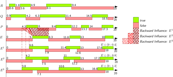
Figure 6: Truths of Predicates={P,Q,R,E} and Pseudo-Targets (n=3, k=0.4) for $E$.

Definition 15.

Pseudo-Target: A pseudo-target is an artificially created target computed by stretching the truth of the target’s interval set back in time by a multiple of the delay resolution $k$. The target $E$ stretched back in time by an amount $i\times k$ is denoted as $E^{i}$. The interval set for the pseudo-target $E^{i}$ in trace $\mathcal{T}$ is computed as follows:

$$\mathcal{I}_{\mathcal{T}}(E^{i})=\mathcal{I}_{\mathcal{T}}(E)\ominus[0:i\times k]=\bigcup_{I\in\mathcal{I}_{\mathcal{T}}(E)}I\ominus[0:i\times k]$$ (1)

where, the $\ominus$ represents the Minkowski difference between intervals: $[\alpha:\beta]\ominus[a:b]=[\alpha-b:\beta-a]$. The truth intervals for the negated pseudo-targets are computed similarly.∎

For a prefix sequence with at-most $n$ delay intervals and a delay resolution $k$, we augment the truth set, $\mathbb{I}_{\mathcal{T}}(\mathbb{P})$ to $\widehat{\mathbb{I}}_{\mathcal{T}}(\mathbb{P})$ as follows:

$$\widehat{\mathbb{I}}_{\mathcal{T}}(\mathbb{P})=\mathbb{I}_{\mathcal{T}}(\mathbb{P})\cup(\bigcup_{1\leq i\leq n}\mathcal{I}_{\mathcal{T}}(E^{i}))\cup(\bigcup_{1\leq i\leq n}\mathcal{I}_{\mathcal{T}}(\neg E^{i}))$$ (2)

Example 4.

In Figure 6, $n=3$ and $k=0.4$, the truth intervals of three pseudo-targets of predicate $E$ are shown. Pseudo-target $E^{i}$ is computed according to Equation 1. For instance, given $\mathcal{I}_{\tau}(E)=\{[5:8.3),[11.8:13),[18:20)\}$ and $\mathcal{I}_{\tau}(\neg E)=\{[0:5),[8.3:11.8),[13:18)\}$, $\mathcal{I}_{\tau}(E^{2})$ and $\mathcal{I}_{\tau}(\neg E^{2})$ are computed to be as follows:

$$\mathcal{I}_{\tau}(E^{2}) =\{[5:8.3),[11.8:13),[18:20)\}\ominus[0:0.8]$$

$$=\{[4.2:8.3),[11:13),[17.2:20)\}$$

$$\mathcal{I}_{\tau}(\neg E^{2}) =\{[0:5),[8.3:11.8),[13:18)\}\ominus[0:0.8]$$

$$=\{[0:5),[7.5:11.8),[12.2:18)\}\qed$$

Observe that in Figure 6, the true and false intervals for pseudo-targets are not complementary. We wish to mine prefixes to explain both $E$ and $\neg E$. Hence while generating pseudo-targets, Equation 1 is also used to generate the pseudo-target truth intervals for when $E$ is false.

4.3 Effect of Pseudo-Targets on Decision Making

At each decision node, we must decide which predicate best reduces the error in the resulting split, while simultaneously choosing a temporal position for the predicate in the $n$-length prefix sequence. We achieve the latter by choosing to test a predicate with each pseudo-target, to identify which pseudo-target (and therefore which position), given a possibly non-empty partial prefix, is most correlated with the predicate under test. The choice of predicate and position that gives the best correlation is then chosen.

At each query node of the decision tree, with constraint set $\mathcal{C}$, for target $E$, the following steps are carried out:

In the core steps of the above procedure, namely, Step 1 and Step 2, we compute the statistical measures of mean and error for pseudo-targets $\hat{E}$ and $\tilde{E}$. The definition of $Mean_{\mathcal{T}_{\mathcal{C}}}(\hat{E})$ and $Error_{\mathcal{T}_{\mathcal{C}}}(\hat{E})$ in Section 4.1 assume that the true and false interval lists of $E$ are compliments of each other, however, for a pseudo-target $\hat{E}$ this is not true, hence the metrics cannot be directly applied. Furthermore, even though in each iteration of Step 2, a choice of $\langle P,i\rangle$ is made, it is unclear for which pseudo-target the measures must be computed. We first resolve the later and then address the computation of the statistical measures.

Note that in Step 2 (a), for a predicate $P$, once a pseudo-target position is determined, the split considers $P$ being true in one branch and $P$ being false in the other, while the temporal position for $P$ and $\neg P$ remains the same for both child nodes of the split.

4.3.1 Choosing a Pseudo-Target for a Partial Prefix

A path of a decision tree in the making is expanded by adding a constraint $\langle P,i\rangle$ into the constraint set $\mathcal{C}$ corresponding to the path. The choice of the constraint, namely the predicate $P$ and its bucket $\sqcup_{i}$, is made by comparing the influence (on the target, $E$) of the prefix sequences obtained by adding to $\mathcal{C}$ each such pair $\langle P,i\rangle$. At the heart of this approach are the metrics used to determine the goodness of a partial prefix sequence in terms of its influence on the target $E$. Our metrics are computed by stretching the target back in time as pseudo-targets. It is, therefore, an important step to determine which of the pseudo-targets is to be used for a given partial prefix sequence.

Proposition 1.

The pseudo-target applicable for a given constraint set $\mathcal{C}$ is the smallest bucket position, $i$, among all non-empty buckets, $0\leq i\leq n$. ∎

Example 5.

For $n=3$, and delay resolution $k=0.4$, we consider the template of the form: $\sqcup_{3}$ ##[0:0.4] $\sqcup_{2}$ ##[0:0.4] $\sqcup_{1}$ ##[0:0.4] $\sqcup_{0}$ |-> E. Suppose the given constraint set is $\mathcal{C}=\{\langle Q,3\rangle,\langle P,1\rangle\}$. The prefix-buckets are therefore, $\mathcal{B}_{3}(\mathcal{C})=\{Q\}$, $\mathcal{B}_{2}(\mathcal{C})=\{\}$, $\mathcal{B}_{1}(\mathcal{C})=\{P\}$ and $\mathcal{B}_{0}(\mathcal{C})=\{\}$. The partial prefix sequence that results from $\mathcal{C}$ is $\mathcal{S}\equiv$ $Q$ ##[0:0.8] $P$. This then asserts $Q$ ##[0:0.8] $P$ |-> ##[0:0.4] $E$.

Note that the delays separating placeholders $\sqcup_{3}$, $\sqcup_{2}$, and $\sqcup_{1}$ have merged into the interval ##[0:0.8] because $\sqcup_{2}$ is empty. Also, since $\sqcup_{0}$ is empty, the delay between $\sqcup_{1}$ and $\sqcup_{0}$ separates $\mathcal{B}_{1}(\mathcal{C})$ from $E$. In this case, therefore, evaluating $\mathcal{C}$ requires using pseudo-target $E^{1}$ as shown in Figure 6. In other words, $E^{1}$ represents the expression ##[0:0.4]$E$. ∎

4.3.2 Adapting Statistical Measures for Pseudo-Targets

Standard decision tree algorithms assume that classes are independent and that no data point in the data set belongs to more than one class. However, for a pseudo-target, this is not the case, because, the pseudo-target can (non-deterministically in time) be true and false at some times (see Figure 6). Hence a traditional error computation, such as in Definition 13, misrepresents the relationships that exist.

Furthermore, at each decision node, we make two decisions, deciding which predicate to pick, and deciding which temporal position (pseudo-target) gives the best gain for the chosen predicate. The two decisions are dependent and must be made together. Pseudo-targets help us to learn the most influential temporal position for a predicate.

Example 6 demonstrates the lacunae of using the traditional definitions of mean and error from Section 4.1.

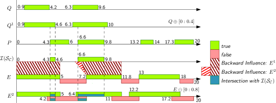
Figure 7: Predicates={Q,P,E} and Pseudo-Targets (n=3, k=0.4) for $E$. $\mathcal{C}=\{\langle Q,3\rangle,\langle P,2\rangle\}$ is a constraint set; while $\mathcal{I}(\mathcal{S}_{\mathcal{C}})$ is the set of end match influence time intervals.

Example 6.

Consider the constraint set $\mathcal{C}=\{\langle Q,3\rangle,\langle P,2\rangle\}$, where the truth intervals of the predicates are shown in Figure 7. We demonstrate the computation of $Mean_{\mathcal{T}_{\mathcal{C}}}({E^{2}})$ and $Error_{\mathcal{T}_{\mathcal{C}}}({E^{2}})$ for $\mathcal{C}$, following their standard definitions over time intervals, as given in Section 4.1.

• $\mathcal{S}_{\mathcal{C}}$ $\equiv$ $Q$ ##[0:0.4] $P$. The influence set is computed following Definition 10:

  $$\mathcal{I}(\mathcal{S}_{\mathcal{{C}}}) =\{[4.3:4.6),[6.6:9.8)\}$$

  $$|\mathcal{I}(\mathcal{S}_{{\mathcal{C}}})| =(4.6-4.3)+(9.8-6.6)=3.5$$

Since the smallest non-empty bucket is $\sqcup_{2}$ (containing $P$), we use pseudo-target $E^{2}$ in our computations. The mean and error with respect to $E^{2}$ are computed as follows:

$$\mu_{\mathcal{T}_{{\mathcal{C}}}}({E^{2}}) =\frac{|\mathcal{I}_{{\mathcal{T}_{{\mathcal{C}}}}}(E^{2})\cap\mathcal{I}(\mathcal{S}_{\hat{\mathcal{C}}})|}{|\mathcal{I}(\mathcal{S}_{{\mathcal{C}}})|} \mu_{\mathcal{T}_{{\mathcal{C}}}}({\neg E^{2}}) =\frac{|\mathcal{I}_{{\mathcal{T}_{{\mathcal{C}}}}}(\neg E^{2})\cap\mathcal{I}(\mathcal{S}_{{\mathcal{C}}})|}{|\mathcal{I}(\mathcal{S}_{{\mathcal{C}}})|}$$

$$=\frac{(0.3+3.2)}{(3.5)}=\frac{(3.5)}{(3.5)} =\frac{(0.3+0.8)}{(3.5)}=\frac{(1.1)}{(3.5)}$$

$$={1.0} ={0.3143}$$

$$\epsilon_{\mathcal{T}_{{\mathcal{C}}}}({E^{2}}) =-(0)-(-0.5238) =0.5238$$

Observe that for the prefix $\mathcal{S}_{\mathcal{C}}$, visually one observes no error with respect to $E^{2}$ (indicated by the blue band overlayed on $E^{2}$). Hence, intuitively, the property $Q$ ##[0:0.4] $P$ |-> ##[0:0.8] $E$, having no error, should be reported. However, since error exists with respect to $\neg E^{2}$, according to Definition 13 the property is would be set aside as requiring refinement, by adding predicates in some bucket.∎

From Example 6 it is clear that using the measures of mean and error from Section 4.1, it is possible to miss potential relations that may exist in the data presented in Figure 7. This is primarily due to the fact that the measures ignore that there can be an overlap of the truth intervals of a pseudo-target’s true and false state. The measure of error counts the entropy contributed by the overlapping states twice. We introduce the definition of unified error that takes this into account when computing the error.

Definition 16.

Unified-Error${}_{\mathcal{T}}(E^{i},C)$: For the target class $E^{i}$, the unified error, denoted as $UE_{\mathcal{T}_{\mathcal{C}}}(E^{i})$, for the trace $\mathcal{T}$ constrained by $\mathcal{C}$ is defined as follows:

$$UE_{\mathcal{T}_{\mathcal{C}}}(E^{i})=\epsilon_{\mathcal{T}_{\mathcal{C}}}(E^{i})+\mu_{\mathcal{T}_{\mathcal{C}}}(E^{i}\wedge\neg E^{i})\times log_{2}(\mu_{\mathcal{T}_{\mathcal{C}}}(E^{i}\wedge\neg E^{i}))\qed$$

While computing the unified error, the term $\mu_{\mathcal{T}_{\mathcal{C}}}(E^{i}\wedge\neg E^{i})\times log_{2}(\mu_{\mathcal{T}_{\mathcal{C}}}(E^{i}\wedge\neg E^{i})$ represents the entropy in the region of the overlap. By adding this term, we effectively ensure that the entropy from the overlap is considered only once when computing the unified error.

Lemma 3.

For a PSI-L property, the unified error, $UE_{\mathcal{T}_{\mathcal{C}}}(E^{i})$, for constraint set $\mathcal{C}$ and consequent pseudo-target $E^{i}$ is zero if and only if $\mathcal{C}$ decides $E^{i}$ or $\neg E^{i}$, that is, there are no counter-examples for $\mathcal{S}_{\mathcal{C}}$|->$E^{i}$ or there are no counter-examples for $\mathcal{S}_{\mathcal{C}}$|->$\neg E^{i}$.

Proof.

We make the assumption that $|\mathcal{I}(\mathcal{S}_{\mathcal{C}})|>0$, the sum of lengths of truth intervals for the expression describing $\mathcal{C}$ is non-zero. For the case where $i=0$, since $\mu_{\mathcal{T}_{\mathcal{C}}}(E\wedge\neg E)=0$, $UE_{\mathcal{T}_{\mathcal{C}}}(E^{0})=\epsilon_{\mathcal{T}_{\mathcal{C}}}(E)$. We therefore, only consider the case when $i>0$.

Part A: Consider the property $\mathcal{S}_{\mathcal{C}}$|->$E^{i}$, where $|\mathcal{I}_{\mathcal{T}}(E^{i})\cap\mathcal{I}(\mathcal{S}_{\mathcal{C}})|>0$. Assume that there are counter-examples for $\mathcal{S}_{\mathcal{C}}$|->$E^{i}$. The counter-examples would introduce a non-zero time interval when $\mathcal{S}_{\mathcal{C}}$ is true and $E^{i}$ is false. Let one of the counter-example time-intervals be the interval $[a:b)$, where $b>a$. Therefore, $|\mathcal{I}_{\mathcal{T}}(\neg E^{i})\cap\mathcal{I}(\mathcal{S}_{\mathcal{C}})|>0$, hence $\mu_{\mathcal{T}_{\mathcal{C}}}(\neg E^{i},C)>0$, and $log_{2}(\mu_{\mathcal{T}_{\mathcal{C}}}(\neg E^{i},\mathcal{C})))<0$ (the mean is bounded between 0 and 1). Similarly the term, $\mu_{\mathcal{T}_{\mathcal{C}}}(E^{i},\mathcal{C})\times log_{2}(\mu_{\mathcal{T}_{\mathcal{C}}}(E^{i},\mathcal{C}))<0$, since $|\mathcal{I}_{\mathcal{T}}(\neg E^{i})\cap\mathcal{I}(\mathcal{S}_{\mathcal{C}})|>0$ . Hence, from Definition 13, $Error_{\mathcal{T}}(E^{i},\mathcal{C})>0$. For $i>0$, $\mu_{\mathcal{T}_{\mathcal{C}}}(E^{i}\wedge\neg E^{i})>0$, however $\mu_{\mathcal{T}_{\mathcal{C}}}(E^{i}\wedge\neg E^{i})<\mu_{\mathcal{T}_{\mathcal{C}}}(\neg E^{i})$. Therefore, $\epsilon_{\mathcal{T}_{\mathcal{C}}}(E^{i})>\mu_{\mathcal{T}_{\mathcal{C}}}(E^{i}\wedge\neg E^{i})\times log_{2}(\mu_{\mathcal{T}_{\mathcal{C}}}(E^{i}\wedge\neg E^{i}))$, and hence $UE_{\mathcal{T}_{\mathcal{C}}}(E^{i})>0$ .

Consider the property $\mathcal{S}_{\mathcal{C}}$|->$E^{i}$, where $|\mathcal{I}_{\mathcal{T}}(E^{i})\cap\mathcal{I}(\mathcal{S}_{\mathcal{C}})|=|\mathcal{I}(\mathcal{S}_{\mathcal{C}})|$. Let $\Upsilon=\mathcal{I}_{\mathcal{T}}(E^{i})\cap\mathcal{I}_{\mathcal{T}}(\neg E^{i})$ represent the overlapping intervals of $E^{i}$ and $\neg E^{i}$. Since, $|\mathcal{I}_{\mathcal{T}}(E^{i})\cap\mathcal{I}(\mathcal{S}_{\mathcal{C}})|=|\mathcal{I}(\mathcal{S}_{\mathcal{C}})|$, $\mathcal{I}(\mathcal{S}_{\mathcal{C}})\subseteq\mathcal{I}_{\mathcal{T}}(E^{i})$. Therefore, $\mathcal{I}_{\mathcal{T}}(\neg E^{i})\cap\mathcal{I}(\mathcal{S}_{\mathcal{C}})\subseteq\mathcal{I}_{\mathcal{T}}(E^{i})$ and hence $\mathcal{I}_{\mathcal{T}}(\neg E^{i})\cap\mathcal{I}(\mathcal{S}_{\mathcal{C}})=\Upsilon\cap\mathcal{I}(\mathcal{S}_{\mathcal{C}})$. For $i>0$, $\Upsilon\neq\emptyset$, and $0\leq|\Upsilon\cap\mathcal{I}(\mathcal{S}_{\mathcal{C}})|<|\mathcal{I}(\mathcal{S}_{\mathcal{C}})|$. Hence, for the case where $|\Upsilon\cap\mathcal{I}(\mathcal{S}_{\mathcal{C}})|=0$, $\mu_{\mathcal{T}_{\mathcal{C}}}(\neg E^{i},C)=\mu_{\mathcal{T}_{\mathcal{C}}}(E^{i}\wedge\neg E^{i},C)=0$. On the other hand, when $|\Upsilon\cap\mathcal{I}(\mathcal{S}_{\mathcal{C}})|>0$, $\mu_{\mathcal{T}_{\mathcal{C}}}(\neg E^{i},C)=\mu_{\mathcal{T}_{\mathcal{C}}}(E^{i}\wedge\neg E^{i},C)$ and the term for $\neg E$ in $\epsilon_{\mathcal{T}_{\mathcal{C}}}(E^{i})$ balances out the term for $\Upsilon$ from $UE_{\mathcal{T}_{\mathcal{C}}}(E^{i})$, yielding a unified error of zero.

The proof for when the property if of the form $\mathcal{S}_{\mathcal{C}}$|->$\neg E^{i}$ is identical.

Part B: Conversely, if the unified error is non-zero, then $0<\mu_{\mathcal{T}_{\mathcal{C}}}(E^{i},\mathcal{C})<1$ and $0<\mu_{\mathcal{T}_{\mathcal{C}}}(\neg E^{i},\mathcal{C})<1$. If any one term was zero or one, the same argument, using overlapping truth intervals, $\Upsilon$, from Part A of the proof would render the error zero. From Definition 12, $0<\mu_{\mathcal{T}_{\mathcal{C}}}(E^{i},\mathcal{C})<1$, $0<\mu_{\mathcal{T}_{\mathcal{C}}}(\neg E^{i},\mathcal{C})<1$, and hence $\mathcal{I}_{\mathcal{T}}(E^{i})\cap\mathcal{I}(\mathcal{S}_{\mathcal{C}})\neq\mathcal{I}(\mathcal{S}_{\mathcal{C}})$ and $\mathcal{I}_{\mathcal{T}}(\neg E^{i})\cap\mathcal{I}(\mathcal{S}_{\mathcal{C}})\neq\mathcal{I}(\mathcal{S}_{\mathcal{C}})$. Therefore, there exists a non-empty interval $[a_{1}:b_{1})$, $b_{1}>a_{1}$ where $\mathcal{S}_{\mathcal{C}}$ is true and $E^{i}$ is false, and there exists a non-empty interval $[a_{2}:b_{2})$, $b_{2}>a_{2}$ where $\mathcal{S}_{\mathcal{C}}$ is true and $E^{i}$ is true, respectively representing counter-example intervals for $\mathcal{S}_{\mathcal{C}}$|->$E^{i}$ and $\mathcal{S}_{\mathcal{C}}$|->$\neg E^{i}$. ∎

Example 7.

In Example 6 on considering the overlap component and computing the Unified Error for the constraint set $\mathcal{C}$, we get the following:

$$\mu_{\mathcal{T}_{{\mathcal{C}}}}({E^{2}\wedge\neg E^{2}}) =\frac{|\mathcal{I}_{{\mathcal{T}_{\mathcal{C}}}}(E^{2}\wedge\neg E^{2})\cap\mathcal{I}(\mathcal{S}_{\mathcal{C}})|}{|\mathcal{I}(\mathcal{S}_{\mathcal{C}})|} UE_{\mathcal{T}_{\mathcal{C}}}(E^{2}) =\epsilon_{\mathcal{T}_{{\mathcal{C}}}}({E^{2}})+0.3143\times(log_{2}(0.3143))$$

$$=\frac{(0.3+0.8)}{(3.5)}=\frac{(1.1)}{(3.5)}~{}~{} =0.5238~{}+~{}(-0.5238)$$

$$={0.3143} ={0}$$

From this example, we see that the use of Unified Error reveals the association in the data that was earlier set aside when using the error metric of Definition 13. ∎

The non-determinism resulting out of reasoning with time intervals presents another fundamental difference with the traditional decision tree learning algorithm. Each node in the traditional decision tree splits the data points into disjoint subsets, which is leveraged by the information gain metric. As the following example shows, some time points in the time-series data may be relevant for both branches of a node in the decision tree.

Example 8.

Consider the split of the data-set resulting from considering $Q$ at bucket $\sqcup_{3}$ to augment the constraint set $\{\langle P,2\rangle\}$ to obtain ${\mathcal{C}}_{0}=\{\langle\neg Q,3\rangle,\langle P,2\rangle\}$ and ${\mathcal{C}}_{1}=\{\langle Q,3\rangle,\langle P,2\rangle\}$. Due to the non-deterministic semantics of the temporal operator ##[$a:b$], the forward influence (end-matches) of ${\mathcal{C}}_{0}$ and ${\mathcal{C}}_{1}$ overlap.

$$\mathbb{F}(\mathcal{S}_{{\mathcal{C}}_{0}},\mathcal{W}_{2}^{3}) =\{[4.3:6),[6.6:6.7),[9.6:9.8),[13.2:14),[17.3:20)\}$$

$$\mathbb{F}(\mathcal{S}_{{\mathcal{C}}_{1}},\mathcal{W}_{2}^{3}) =\{[4.3:4.6),[6.6:9.8)\}$$

The two sets overlap at all time-points in the intervals $[4.3:4.6)$, $[6.6:6.7)$ and $[9.6:9.8)$. Hence, the sum of the weights in the definition of Gain in Definition 14 exceeds $1$, that is:

$$\frac{|\mathbb{F}(\mathcal{S}_{{\mathcal{C}}_{0}},\mathcal{W}_{2}^{3})|}{|\mathcal{I}(\mathcal{S}_{\{\langle P,2\rangle\}})|}+\frac{|\mathbb{F}(\mathcal{S}_{{\mathcal{C}}_{1}},\mathcal{W}_{2}^{3})|}{|\mathcal{I}(\mathcal{S}_{\{\langle P,2\rangle\}})|}>1$$

Furthermore, the influence set of intervals for the constraint set $\{\langle P,2\rangle\}$ is:

$$\mathcal{I}(\mathcal{S}_{\{\langle P,2\rangle\}})=\{[4.3:6),[6.6:9.8),[13.2:14),[17.3:20)\}$$

Since the temporal position of $Q$ is earlier than that of $P$, $\mathbb{F}(\mathcal{S}_{{\mathcal{C}}_{0}},\mathcal{W}_{2}^{3})\cup\mathbb{F}(\mathcal{S}_{{\mathcal{C}}_{1}},\mathcal{W}_{2}^{3})=\mathcal{I}(\mathcal{S}_{\{\langle P,2\rangle\}})$, however, this need not always be the case. If $Q$ is placed later than $P$ in the sequence, the forward influence list can change substantially, since it would now be contained in the interval list of $Q$. ∎

Due to both, potential overlapping data-points between the child nodes of a split and the data-points after the split being potentially different from those of the parent node, we present a revised definition of gain, called unified gain.

Definition 17.

Unified-Gain: The gain (improvement in error) of choosing to split on $P\in\mathbb{P}$, at bucket position $b$, given the existing constraint set $\mathcal{C}$, at a node having error $\epsilon$, is as follows:

$$UG(\epsilon,\mathcal{C},P,b)=\epsilon-\alpha(\mathcal{C},P,b)\times\epsilon_{\mathcal{T}_{\mathcal{C}\cup\{\langle P,b\rangle\}}}(E)-\alpha(\mathcal{C},\neg P,b)\times\epsilon_{\mathcal{T}_{\mathcal{C}\cup\{\langle\neg P,b\rangle\}}}(E)$$

where,

$$\alpha(\mathcal{C},P,b)=\frac{|\mathcal{I}_{\mathcal{T}}(\mathcal{S}_{\mathcal{C}\cup\{\langle P,b\rangle\}})|}{|\mathcal{I}_{\mathcal{T}}(\mathcal{S}_{\mathcal{C}\cup\{\langle P,b\rangle\}})|+|\mathcal{I}_{\mathcal{T}}(\mathcal{S}_{\mathcal{C}\cup\{\langle\neg P,b\rangle\}})|}\qed$$

4.4 Variations of Unified Gain with Temporal Positions

Given an existing constraint set $\mathcal{C}$ (possibly empty - at the root of the tree), a candidate predicate $P$, and its temporal position $i$ in the sequence, the Gain is dependent on the resulting pseudo-target association.

Theorem 1.

The Unified Gain, of placing predicate $P$ in bucket index $i$, is monotonically non-decreasing with increasing values of $i$.

Proof.

Following Proposition 1, the pseudo-target association is dependent on the smallest index among the non-empty buckets in the constraint lists resulting from the split. The split results in two nodes, one with the constraint list $\mathcal{C}\cup\{\langle P,i\rangle\}$ and the other with the constraint list $\mathcal{C}\cup\{\langle\neg P,i\rangle\}$. The smallest non-empty bucket is, therefore, the minimum of $i$ and the index of the smallest index non-empty bucket in $\mathcal{C}$. Let the index of the smallest index non-empty bucket in $\mathcal{C}$ be $b$. Let $\hat{b}$ be the lesser of $i$ and $b$. The length of interval list for the pseudo-target, $|\mathcal{I}(E^{\hat{b}})|$, becomes larger with larger values of $\hat{b}$ (From Definition 15).

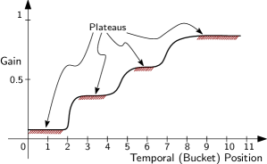
Figure 8: Gain for a candidate predicate, with varying temporal distances from the target predicate.

Initially, at the root of the decision tree, the constraint set, $\mathcal{C}$, is empty. Hence, as $\hat{b}$ increases, a larger fraction of the truth of $P$ would be covered by the pseudo-target $E^{\hat{b}}$. This would cause the quantum of counter-examples for both true and false states of $P$ and it’s association with $E$ to reduce, leading to a reduced entropy, and therefore an increase in Gain. Hence as $\hat{b}$ increases, the Gain would monotonically increase or remain stagnant at a plateau. This is depicted in Figure 8.

When the constraint set, $\mathcal{C}$, is non-empty, i.e. there is at least one element $\langle Q,j\rangle\in\mathcal{C}$, the following cases arise:

1. [$b>i$] (Figure 9) : The end-match of the sequence $C\cup\langle P,i\rangle$ is computed by adding $[0:(b-i)\times k]$ to the end-match of $\mathcal{C}$. While maintaining $i<b$, as $i$ increases, i.e. $i$ is a bucket further from the target, but closer to the end-match of $\mathcal{C}$ (depicted in Figure 9), the length of the end-match of the resulting constraint-set $C\cup\langle P,i\rangle$, monotonically decreases. For larger differences between $b$ and $i$ (smaller values of $i$), the end-match is wider, hence the potential for counter-examples (with respect to the target) is higher. Therefore, as $i$ increases, the entropy monotonically decreases.

   

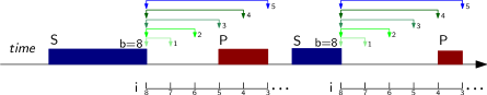
   Figure 9: Relative Position of Predicate $P$ with respect to the end-match interval list for a constraint set, with the end-match represented as $\mathcal{S}$. The index of the minimum index non-empty bucket, $b$, is 8. The index of the bucket where $P$ may be placed in the sequence is $i$.

   

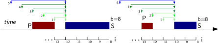
   Figure 10: Relative Position of Predicate $P$ with respect to the end-match interval list for a constraint set, with the end-match represented as $\mathcal{S}$. The index of the minimum index non-empty bucket, $b$, is 8. The index of the bucket where $P$ may be placed in the sequence is $i$.

2. [${b}\leq i$] (Figure 10) : For constraint-set $\mathcal{C}$, either $\mathcal{B}_{i}$ is empty or non-empty. When $P$ is placed in bucket $i\geq b$, the new bucket $\mathcal{B}^{\prime}_{i}=\mathcal{B}_{i}\cup\{P\}$. We have the following two cases:

   1. $\mathcal{B}_{i}$ is non-empty: On adding $P$ to bucket $i$, let The interval list of $P$ is intersected with the interval list of $\mathcal{B}_{i}$ and therefore the resulting bucket has the interval list $\mathcal{I}(\mathcal{B}^{\prime}_{i})\subseteq\mathcal{I}(\mathcal{B}_{i})$.

   2. $\mathcal{B}_{i}$ is empty: Let $h$ be the smallest bucket index, $h>i$, such that $\mathcal{B}_{h}\neq\emptyset$, and let $j$ be the largest bucket index, $j<i$, such that $\mathcal{B}_{j}\neq\emptyset$. If such a index $h$ does not exist, then $i$ is the largest index non-empty bucket in the prefix, while the case that $j$ does not exist is not possible under the present case ($b\leq i$).

      If $\mathcal{B}_{h}\neq\emptyset$, then the forward influence of $\mathcal{B}_{h}$ on $\mathcal{B}_{j}$ is computed as follows:

      $$\Theta=(\mathcal{I}(\mathcal{B}_{h})\oplus[0:(h-j)\times k])\cap\mathcal{I}(\mathcal{B}_{j})$$

      However, on adding $P$ in bucket $i$, $h>i>j$, the forward influence of $\mathcal{B}_{h}$ on $\mathcal{B}_{j}$ is computed as follows:

      $$\Omega=((\mathcal{I}(\mathcal{B}_{h})\oplus[0:(h-i)\times k])\cap\mathcal{I}(\mathcal{B}_{i}))\oplus[0:(i-j)\times k])\cap\mathcal{I}(\mathcal{B}_{j})$$

      Hence, $\Omega\subseteq\Theta$. The potentially reduced forward influence on $\mathcal{B}_{j}$ similarly propagates toward reducing the end-match for the sequence having $P$ in bucket $i$. A reduced end-match has lesser potential for entropy, and therefore yields a higher gain, or leaves the gain unchanged. ∎

4.5 A Miner for Prefix Sequences

The prefix sequence inference mining algorithm is presented as Algorithm 1. The length of the sequence $n$, and the delay resolution $k$ are meta-parameters of the algorithm. Every choice of $n$ and $k$ yields a different instance of the algorithm. The choice of values of the meta-parameters must come from the domain. The algorithm learns a decision tree for PSI properties for the truth set $\widehat{\mathbb{I}}_{\mathcal{T}}(\mathbb{P})$ for a choice of $n$ and $k$.

Input: Truth Set $\mathbb{I}_{\mathcal{T}}(\mathbb{P})$ for trace $\mathcal{T}$, Predicate List $\mathbb{P}$, Target $E$, Constraint List $\mathcal{C}$

Output: PSI-L properties $\mathbb{A}$, structured as the decision tree.

1

2if stoppingCondition($\mathbb{I}_{\mathcal{T}}(\mathbb{P}),\mathbb{P},E,\mathcal{C}$) then  return;

3

4$b\leftarrow$ Smallest non-empty bucket position in $\mathcal{C}$;

5

6$P_{best}\leftarrow\emptyset$; $i_{best}\leftarrow-1$; $g_{best}\leftarrow 0$;

7

8for $0\leq i<n$ do

9       forall $P\in\mathbb{P},\langle P,i\rangle\notin\mathcal{C}$ do

10             $g\leftarrow UG(UE_{\mathcal{T}_{\mathcal{C}}}(E^{b}),\mathcal{C},P,i)$;

11            if $g>g_{best}$ then  $P_{best}\leftarrow P$; $i_{best}\leftarrow i$; $g_{best}\leftarrow g$ ;

12            

13      

14if $i_{best}<0$ then  return;

15 nk-PSI-Miner$(\mathbb{I}_{\mathcal{T}}(\mathbb{P}),\mathbb{P},E,\mathcal{C}\cup\{\langle P_{best},i_{best}\rangle\})$;

16 nk-PSI-Miner$(\mathbb{I}_{\mathcal{T}}(\mathbb{P}),\mathbb{P},E,\mathcal{C}\cup\{\langle\neg P_{best},i_{best}\rangle\})$;

ALGORITHM 1 nk-PSI-Miner: Mining n-length, k-resolution Prefix Sequences

In Algorithm 1, Line 1 tests the current node for termination. One of the criteria for termination is that the node is homogeneous with respect to $E$, that is, the error at the node is zero. Other stopping conditions are described later in Section 6.

In Line 1 the smallest non-empty bucket index is identified from the constraint set $\mathcal{C}$, and is used in Line 1 to compute the error for $\mathcal{C}$. The loop at Line 1 iterates over every pseudo-target position, while Line 1 chooses a predicate from the predicate alphabet $\mathbb{P}$. Any predicate and pseudo-target position combination already present in $\mathcal{C}$ are ignored in Line 1. The Unified Gain for the choice of predicate and pseudo-target is computed in Line 1 and the best gain, and its associated arguments are determined in Line 1. The computation of Unified Gain uses the smallest non-empty bucket index for the choice of pseudo-target, with respect to which the Unified Entropy and Unified Gain are computed. The loop beginning at Line 1 implicitly chooses the smallest bucket position for the “best predicate” that has the maximum gain. As shown in Section 4.4, the gain plateaus at various points and we choose the earliest point on the plateau that has the highest gain. Line 1 terminates exploration if for the current node, no remaining predicate and bucket position pair can improve the solution. If a best predicate and bucket position pair is found, lines 1 and 1 branch on new constraint sets. In the following section, we describe an approach for translating a decision tree constructed using Algorithm 1 into properties in PSI-L.

4.6 From Decision Trees to PSI-L Formulae

The nodes in the decision tree at which the error is zero are the leaf nodes of the tree and have homogeneous data with respect to the truth of $E$. We call these nodes PSI nodes and the labels along the path from a PSI node to the root (the constraint set $\mathcal{C}$) form a PSI-L property template. A template consists of predicates and their relative sequence position from the target. Concretizing the PSI template involves computing the relative positions of predicates from each other. We do this by grouping predicates that fall in the same relative temporal position into a bucket, and then compute tight time delays that separate buckets in order of their temporal distance from the target $E$. The computation of tight separating intervals between buckets assumes an any-match (may) semantic.

At a PSI node, the set of constraints $\mathcal{C}$ is known. Recall, that a PSI node is a node at which the entropy is zero. We use the notation $\mathcal{B}_{i}$, to denote the set of predicates having influence on the target with a step size of $[0:i\times k]$, while $s_{i}$ is the conjunction of predicates in $\mathcal{B}_{i}$. The PSI-L property has one of the following forms:

$s_{n}~{}\tau_{n}~{}s_{n-1}~{}\tau_{n-1}\ldots\tau_{1}~{}s_{0}$|-> $E$	, when $\mathcal{B}_{0}\neq\emptyset$
$s_{n}~{}\tau_{n}~{}s_{n-1}~{}\tau_{n-1}\ldots\tau_{2}~{}s_{1}$|-> $\tau_{1}~{}E$	, otherwise

We wish to compute tight intervals, $\tau_{i}$, $1\leq i\leq n$.

Definition 18.

Tight delay separation: For trace $\mathcal{T}$ and constraint set $\mathcal{C}$, a delay separation $[a:b]$, $a\leq b$, between buckets $\mathcal{B}_{i}$ and $\mathcal{B}_{j}$, $i>j$, is tight with respect to the match semantics of Definition 2 iff the following conditions hold,

• Maximality: $\exists t_{i},t^{\prime}_{i}\in\mathcal{I}_{\mathcal{T}_{\mathcal{C}}}(\mathcal{B}_{i}),$ $t_{j},t^{\prime}_{j}\in\mathcal{I}_{\mathcal{T}_{\mathcal{C}}}(\mathcal{B}_{j})$: $t_{i}+a=t_{j}$ and $t^{\prime}_{i}+b=t^{\prime}_{j}$

• Left-Tight: If $a>0$, $\forall t\in[0:a);~{}t_{i}\in\mathcal{I}_{\mathcal{T}_{\mathcal{C}}}(\mathcal{B}_{i});~{}t_{j}\in\mathcal{I}_{\mathcal{T}_{\mathcal{C}}}(\mathcal{B}_{j})$: $t_{i}+t\neq t_{j}$

• Right-Tight: If b$<$(i$-$j)$\times$k, $\forall t\in($b,(i$-$j)$\times$k$]$; $t_{i}\in\mathcal{I}_{\mathcal{T}_{\mathcal{C}}}(\mathcal{B}_{i});~{}t_{j}\in\mathcal{I}_{\mathcal{T}_{\mathcal{C}}}(\mathcal{B}_{j})$: $t_{i}+t\neq t_{j}$ ∎

We use the standard interval widening operation for a set of intervals $\mathcal{I}$.

Definition 19.

Widening over a set of intervals: For a set of intervals $\mathcal{I}$, the widening over the intervals in $\mathcal{I}$ is defined to be the following interval:

$$\mathcal{W}(\mathcal{I})=[\min_{I\in\mathcal{I}}l(I)~{}:~{}\max_{I\in\mathcal{I}}r(I)]\qed$$

In the remainder of this section we describe how tight delay separations, or simply separations, are computed. For the property $\mathcal{S}$|->$E^{i}$ we compute separations between buckets. The interval set for the $j^{th}$ bucket, $\mathcal{B}_{j}$, for the constraint set $\mathcal{C}$, of intervals that take part in the prefix $\mathcal{S}_{\mathcal{C}}$, is as follows:

$\dot{\mathcal{I}}_{\mathcal{T}_{\mathcal{C}}}(\mathcal{B}_{j})=\mathds{B}(\mathcal{S},\mathbb{W},j)$

Note, that for the bucket with the smallest index (closest to the target), the intervals taking part in the prefix $\mathcal{S}_{\mathcal{C}}$ are the end-match intervals.

We compute the separation interval, $Sep_{\mathcal{C}}(\mathcal{B}_{j},E)$, for $j>0$, of $\mathcal{B}_{j}$ from $E$ as follows:

• For each interval $\dot{I}_{\mathcal{B}_{j}}$ in $\dot{\mathcal{I}}_{\mathcal{T}_{\mathcal{C}}}(\mathcal{B}_{j})$, and each truth interval $I_{E^{i}}$ of $E$, compute the influence of $\dot{I}_{\mathcal{B}_{j}}$ on $I_{E}$. For some $\dot{I}_{\mathcal{B}_{j}}$ and $I_{E}$, this is given as, $\mathcal{F}^{+}=(\dot{I}_{\mathcal{B}_{j}}\oplus[0:j\times k])\cap I_{E}$.

• For a given $\dot{I}_{\mathcal{B}_{j}}$ and $I_{E}$, and therefore a value of $\mathcal{F}^{+}$, we compute the separation of $\mathcal{F}^{+}$ from $\dot{I}_{\mathcal{B}_{j}}$ as, $\mathcal{D}=\mathcal{F}^{+}\ominus\dot{I}_{\mathcal{B}_{j}}$.

• We compute $\mathcal{D}$ over all combinations of $\dot{\mathcal{I}}_{\mathcal{B}_{j}}$ and $I_{E}$, and widen over the resulting set of intervals.

• It is possible for $\mathcal{D}$ to be larger than $[0:j\times k]$ due to the semantics of the Minkowski operators. We, therefore, bound the widened set by $[0:j\times k]$. In our implementation, intervals in an interval set are sorted according to their timestamps. For any two intervals $[\alpha:\beta]$ and $[a:b]$, we compute the Minkowsky difference between them only if $\beta>=a$.

The separation, $Sep_{\mathcal{C}}(\mathcal{B}_{j},E)$, for $j>0$, of $\mathcal{B}_{j}$ from $E$ as follows:

$Sep_{\mathcal{C}}(\mathcal{B}_{j},E)=\mathcal{W}(I~{}|I=((\dot{I}_{\mathcal{B}_{j}}\oplus[0:j\times k])\cap I_{E})\ominus\dot{I}_{\mathcal{B}_{j}})\cap[0:j\times k]$

Note that $Sep_{\mathcal{C}}(\mathcal{B}_{j},E)$ computes the separation between a bucket $\mathcal{B}_{j}$ and the target $E^{i}$. To form a prefix sequence, delay intervals separating adjacent buckets must be computed. The separation $\tau_{j}$ between $\mathcal{B}_{j}$ and $\mathcal{B}_{j-1}$ is iteratively computed as follows:

$$\tau_{j}=\begin{cases}Sep_{\mathcal{C}}(\mathcal{B}_{i},E)&j=i\\ Sep_{\mathcal{C}}(\mathcal{B}_{j},B_{j-1})&0\leq i<j\leq n\\ \end{cases}$$

Recall that $i$ is the smallest index of a non-empty bucket in $\mathcal{S}_{\mathcal{C}}$, and that some buckets may be empty, and the separation between adjacent non-empty buckets $\mathcal{B}_{j}$ and $\mathcal{B}_{l}$ is computed in a similar manner.

Proposition 2.

Two non-empty buckets $\mathcal{B}_{j}$ and $\mathcal{B}_{l}$ are adjacent iff $\forall m\in(j:l),~{}\mathcal{B}_{m}=\emptyset$. We define the predicate Adj(j,l) to be true iff $\mathcal{B}_{j}$ and $\mathcal{B}_{l}$ are adjacent.

The separation in terms of adjacent buckets is then computed as follows:

$$\tau_{j}=\begin{cases}Sep_{\mathcal{C}}(\mathcal{B}_{j},B_{l})&Adj(j,l),~{}0\leq l<j\leq n\\ Sep_{\mathcal{C}}(\mathcal{B}_{j},E)&j=i\end{cases}$$

The first statement computes the separation between two non-empty adjacent buckets, and the second indicates that the $j^{th}$ bucket is the non-empty bucket in the prefix sequence having the smallest index. Therefore, we use the separation between the $j^{th}$ bucket and the target as-is. The separation between the last non-empty bucket and the target would appear as a delay constraint in the consequent. For a prefix with the largest index bucket being $h$, the second to the smallest being $m$, and the smallest being $i$, the prefix sequence would be of the form, $s_{h}$ $\tau_{h}$ $\ldots$ $\tau_{m}$ $s_{i}$ |-> $\tau_{i}$ $E$.

Example 9.

Consider the set of intervals for two non-empty buckets, $\mathcal{B}_{2}$ and $\mathcal{B}_{3}$, that take part in the match of the prefix, and the interval set for target $E$, to be given as follows:

$$\dot{\mathcal{I}}_{\mathcal{T}_{\mathcal{C}}}(\mathcal{B}_{2}) =\{[4.3:4.6),[6.6:9.8)\}$$

$$\dot{\mathcal{I}}_{\mathcal{T}_{\mathcal{C}}}(\mathcal{B}_{3}) =\{[3.9:4.2),[6.3:6.4)\}$$

$$\mathcal{I}_{\mathcal{T}}(E) =\{[4.6,5),[6.6:6.9),[13:18)\}$$

The delay resolution $k=0.4$. The separation intervals are computed as follows:

• For $\mathcal{B}_{2}$ we compute $Sep_{\mathcal{C}}(\mathcal{B}_{2},E)$ as follows:

  $$\mathcal{F}^{+} =\dot{\mathcal{I}}_{\mathcal{T}_{\mathcal{C}}}(\mathcal{B}_{2})\oplus[0:2\times 0.4]\cap\mathcal{I}_{\mathcal{T}}(E)$$

  $$=\{[4.3:5.4),[6.6:10.6)\}\cap{\mathcal{I}}_{\mathcal{T}}(E)$$

  $$=\{[4.6:5),[6.6:6.9)\}$$

  $$(\mathcal{F}^{+}\ominus I_{\mathcal{B}_{2}})\cap\{[0:0.8]\} =\{[0:0.7),[0:0.3)\}$$

  $$\mathcal{W}(\{[0:0.7),[0:0.3)\}) =[0:0.7]$$

• For $\mathcal{B}_{3}$ we compute $Sep_{\mathcal{C}}(\mathcal{B}_{2},\mathcal{B}_{3})$ as follows:

  $$\mathcal{F}^{+} =(\dot{\mathcal{I}}_{\mathcal{T}_{\mathcal{C}}}(\mathcal{B}_{3})\oplus[0:1\times 0.4])\cap\dot{\mathcal{I}}_{\mathcal{T}_{\mathcal{C}}}(\mathcal{B}_{2})$$

  $$=\{[3.9:4.2),[6.3:6.4)\}\oplus[0:0.4]\cap\dot{\mathcal{I}}_{\mathcal{T}_{\mathcal{C}}}(\mathcal{B}_{2})$$

  $$=\{[4.3:4.6),[6.6:6.8)\}$$

  $$(\mathcal{F}^{+}\ominus I_{\mathcal{B}_{3}})\cap\{[0:0.4]\} =\{[0.1:0.4),[0.2:0.4)\}$$

  $$\mathcal{W}(\{[0.1:0.4),[0.2:0.4)\}) =[0.1:0.4]$$

The property obtained, on integrating the delay separation time intervals, is as follows:$s_{3}$ ##[0.1:0.4] $s_{2}$ |-> ##[0:0.7] E. ∎

5 Quality of Mined PSI-L Properties

The decision tree learned by Algorithm 1 can compute several prefixes. It is important to rank these in terms of those that are likely to be causal relations and those that are not. Furthermore, it is also important to understand how mined prefixes are related to the trace.

We measure the goodness of a PSI-L property $\mathcal{S}$|->$E^{i}$, where $i$ is the smallest non-empty bucket index in $\mathcal{S}$, using heuristic metrics of Support, and Correlation. We also measure how much of the trace is covered for the set of PSI properties generated.

Recall that $E^{i}$ is the $i^{th}$ pseudo-target, that is the target’s truth stretched back in time by an amount of $i\times k$, where $k$ is the delay resolution. In the definitions, while the support only considers $\mathcal{S}$, the correlation and coverage deal with $E^{i}$. To be consistent, we re-enforce in all definitions that we relate the truth of the prefix $\mathcal{S}$ forward in time with target $E$, and hence write $\mathcal{S}$|->$E^{i}$.

Definition 20.

Support: For a property $\mathcal{S}$|->${E^{i}}$, the quantum of time for which $\mathcal{S}$ is true in the trace $\mathcal{T}$ is the support of $\mathcal{S}$|->$E^{i}$.

$$Support(\mathcal{S}\text{\tt|->}E^{i})=\frac{|\mathcal{I}_{\mathcal{T}}(\mathcal{S})|}{||\mathcal{T}||}$$

where $\mathcal{I}_{\mathcal{T}}(\mathcal{S})$ is the influence interval list for the sequence $\mathcal{S}$ computed according to Definitions 10 and 8, while $||\mathcal{T}||$ is the length of the trace given in Definition 1. ∎

A high support for PSI-L property $\mathcal{S}$|->${E^{i}}$ is indicative of $\mathcal{S}$ being frequently true in the trace. However, a low support need not indicate that the property is incorrect, and could indicate a corner case behaviour.

Definition 21.

Correlation: For the assertion $\mathcal{S}$|->${E^{i}}$, correlation indicates how much of $E^{i}$’s truth is associated with $\mathcal{S}$, that is the quantum of the consequent, $E^{i}$’s truth, that the antecedent $\mathcal{S}$ contributes to.

$$Correlation(\mathcal{S}\text{\tt|->}{E^{i}})=\frac{|(\mathcal{I}_{\mathcal{T}}(\mathcal{S})\oplus[0:i\times k])\cap\mathcal{I}_{\mathcal{T}}(E^{i})|}{|\mathcal{I}_{\mathcal{T}}(E^{i})|}\qed$$

Definition 22.

Trace Coverage: Trace coverage quantifies the fraction of the trace that is explained by the properties generated by the miner.

Given a trace $\mathcal{T}$ of length $\mathcal{L}$, and the mined property set $\mathbb{A}$, the coverage interval list of $\mathcal{T}$ by $\mathbb{A}$, denoted $Cov(\mathcal{T},\mathbb{A})$, is computed as follows:

$Cov(\mathcal{T},\mathbb{A})=\bigcup_{(\mathcal{S}\text{{\tt|->}}\tilde{E}^{i})\in\mathbb{A}}(\mathcal{I}_{\mathcal{T}}(\mathcal{S})\oplus[0:i\times k])\cap\mathcal{I}_{\mathcal{T}}(\tilde{E})$

where $\tilde{E}\in\{E,\neg E\}$. The percentage of coverage is then given by $\frac{|Cov(\mathcal{T},\mathbb{A})|}{\mathcal{L}}\times 100$. ∎

Example 10.

We compute the three metrics introduced in this section for the interval sets from the prefix and target from Figure 7.

$$Support(\mathcal{I}_{\mathcal{T}}(\mathcal{S})\text{\tt|->}E^{2}) =\frac{3.5}{20}=17.5\%$$

$$Correlation(\mathcal{I}_{\mathcal{T}}(\mathcal{S})\text{\tt|->}E^{2}) =\frac{|\{[4.3:5.4),[6.6:10.6)\}\cap\{[0:5),[6.4:11.8),[12.2:18)\}|}{|\{[0:5),[6.4:11.8),[12.2:18)\}|}$$

$$=\frac{|\{[4.3:5),[6.6:10.6)\}|}{|\{[0:5),[6.4:11.8),[12.2:18)\}|}$$

$$=\frac{4.7}{16.2}=29.01\%$$

$$Cov(\mathcal{T},\mathbb{A}) =\mathcal{I}_{\mathcal{T}}(\mathcal{S})\oplus[0:2\times 0.8]\cap\mathcal{I}_{\mathcal{T}}(E)$$

$$=\{[4.3:5),[6.6:10.6)\}$$

$$Percentage~{}of~{}coverage =\frac{|\{[4.3:5),[6.6:10.6)\}|}{20}$$

$$=\frac{4.7}{20}=23.5\%\qed$$

6 Stopping Conditions, Over-fitting and Pruning

While building the decision tree, for prefixes, there are two stopping conditions that we employ to terminate the growth of the tree.

1. Purity of a Node: When the constraint set $\mathcal{C}$ completely determines the truth of the target $E$, the decision tree node is 100% pure and further growth is terminated. A node with constraint set $\mathcal{C}$, and minimum bucket position $b$, is considered pure if the unified error at the node is zero, that is $UE_{\mathcal{T}_{\mathcal{C}}}(E^{b})=0$.

2. Depth Constraints: It is also possible to define a depth threshold, $\alpha_{d}$, and stop the tree from growing if the length of the current exploration path crosses $\alpha_{d}$.

Decision trees are known to suffer from problems of over-fitting. Over-fitting involves fitting a learned model so closely to the data, that the model becomes specific in explaining the peculiarities in the data, making it overly defined and specific to the data over which learning is performed. This is exceptionally problematic with data that is discrete. In this case, when dealing with dense real-time data, and arbitrary resolution of time, depending on the time precision in the data, over-fitting can lead to a large number of properties being generated, leaving the designer with an overwhelmingly large number of prefix properties and rendering the mining as an ineffective aid to designers.

To prevent over-fitting, we employ pruning and abstraction mechanisms controlled via meta-parameters. The measures employed are as follows:

1. Using a support threshold: A threshold $\alpha_{s}$ is defined to indicate the minimum support below which a prefix is being over-fit to the data. If a node with constraint set $\mathcal{C}$ has a support below $\alpha_{s}$, further splitting of the node is terminated. Note that, due to the dense interpretation of time, in some situations, a low support is expected when explaining targets concerning corner case behaviours.

2. Using a correlation threshold: A threshold $\alpha_{c}$ is defined to indicate the minimum correlation below which a prefix is being over-fit to the target. If a node with constraint set $\mathcal{C}$ has a correlation below $\alpha_{c}$ with its associated target, further splitting of the node is terminated.

3. Prefix Grouping: We use interval arithmetic to mine prefix sequences. This allows overly constrained prefixes to be grouped into sequences that share common event orderings. Hence a prefix mined by Algorithm 1 may be representative of an infinite number of distinct prefixes that have similar event orderings but dissimilar in delay intervals separating every adjacent pair of events.

4. Constraint Set Limits: Limits on the depth of the decision tree impose an implicit upper bound on the number of constraints used to build a prefix.

The constraints on tree-depth $\alpha_{d}$, support $\alpha_{s}$ and correlation $\alpha_{c}$, are treated as meta-parameters of the decision tree learning algorithm.

7 Handling Multiple Traces

In this article, for simplicity, all metrics have been defined for a single time-series. When considering a set $\mathbb{T}$ of time-series, any pair of time-series may share a common time-line. For instance, consider two autonomous vehicles V1 and tt V2 that have their state recorded over time. The recording for V1 begins at 09:48:07AM and is recorded up to 04:02:23PM. The recording for V2 begins at 08:32:30AM and is recorded up to 04:32:43PM. Hence given a time $t$ in the duration from 09:48:07AM to 04:02:23PM, it is possible that at $t$, we observe two conflicting state entries for a vehicle. Considering truth intervals over predicates, therefore, at any given time, due to differences in the state between V1 and V2, it is possible that a predicate has conflicting values of truth. To resolve this, it is not possible to simply use a timestamp offset and concatenate the two time-series. The concatenation in time could introduce unintended temporal relationships in the data. It is therefore important to treat each time-series as being independent. In this section, we redefine core metrics used in our learning framework for dealing with multiple time-series.

In our framework, the definition of $Mean(.)$ is a fundamental metric, and it is sufficient to re-define this metric to ensure that evidence is considered from all time-series. To handle a set of time-series, the definition of mean is extended as follows:

Definition 23.

Mean${}_{\mathbb{T}_{\mathcal{C}}}$(E): For the target class $E$, the proportion of time that $E$ is true in the set of traces $\mathbb{T}$ constrained by $\mathcal{C}$ :

$$Mean_{\mathbb{T}}(E,\mathcal{C})=\frac{\sum_{\mathcal{T}\in\mathbb{T}}|\mathcal{I}_{\mathcal{T}}(E)\cap\mathcal{I}(\mathcal{S}_{\mathcal{C}})|}{\sum_{\mathcal{T}\in\mathbb{T}}|\mathcal{I}(\mathcal{S}_{\mathcal{C}})|}$$

For convenience, $\mu_{\mathbb{T}_{\mathcal{C}}}(E)$ may be used in place of $Mean_{\mathbb{T}}(E,\mathcal{C})$. The mean is not defined when $\sum_{\mathcal{T}\in\mathbb{T}}|\mathcal{I}(\mathcal{S}_{\mathcal{C}})|=0$. ∎

Similarly, the normalization factor $\alpha$ used in Definition 17 is extended to consider multiple traces as follows:

$$\alpha(\mathcal{C},P,b)=\frac{\sum_{\mathcal{T}\in\mathbb{T}}|\mathcal{I}_{\mathcal{T}}(\mathcal{S}_{\mathcal{C}\cup\{\langle P,b\rangle\}})|}{\sum_{\mathcal{T}\in\mathbb{T}}(|\mathcal{I}_{\mathcal{T}}(\mathcal{S}_{\mathcal{C}\cup\{\langle P,b\rangle\}})|+|\mathcal{I}_{\mathcal{T}}(\mathcal{S}_{\mathcal{C}\cup\{\langle\neg P,b\rangle\}})|)}$$

Using the measures in this section to compute unified entropy and unified gain and associated metrics allows us to incorporate information from multiple time-series.

8 Experimental Results

We use a selection of examples to demonstrate the utility of PSI-Miner. The miner was used on a standard laptop with a 2.40GHz Intel Core i7-5500U CPU with 8GB of RAM.

For each example, we choose meta-parameters $n$, the number of intervals in the antecedent, and $k$, the initial time delay between buckets. The target event, being explained, and the predicate alphabet used for mining are also known. The prefixes learned are validated against the data and prior knowledge that was not available to the miner.

Example 11.

This example focuses on PSI-Miner’s ability to learn and generalize timing intervals across multiple traces. We use position information from multiple vehicles in Town-X (from Section 2, Figure 2) to learn which of the routes from location D to A is the fastest.

There are three routes, namely $DA_{1}$, $DA_{2}$ and $DA_{3}$, in the direction from D to A. We pick time-series of nine vehicles, three from each route. We then run PSI-Miner separately for each route, on its set of three time-series, providing predicates for all way-points. A delay-resolution of $k=2min$ and a maximum sequence length of $n=15$ are used in the experiments. Since a vehicle may spend very little time at the source/destination in relation to total time, we allow small support percentages.

Time to travel from D to A
Route	Property	Support (%)	Correlation (%)
$DA_{1}$	D|-> ##[26.90:28] A	78.56$\times 10^{-2}$	100
$DA_{2}$	D|-> ##[14.21:16] A	26.42$\times 10^{-2}$	100
$DA_{3}$	D|-> ##[18.82:20] A	37.66$\times 10^{-2}$	100
All	D|-> ##[14.21:28] A	51.2$\times 10^{-2}$	100

Table 1: PSI-L Properties describing the time to travel from D to A, along three paths and a summary property for all paths. Time intervals are measured in minutes, with decimals interpreted as a fraction of a minute.

The first three properties in Table 1 describe the time to travel along the three different routes. Note that PSI-Miner picked only one predicate, the one for location D in the antecedent. This is because, for instance, for route $DA_{1}$, D, at the bucket position of 14 (14min$\times$2 = 28min), was sufficient to construct a property. We observe that route $DA_{2}$ is the fastest available route; vehicles leaving D reach A from between 14min:12sec to 16min, while route $DA_{1}$ takes the longest time, that is between 26min:54sec to 28min.

We also evaluate if PSI-Miner is able to correctly generalize this timing information when given time-series from all routes. We provide PSI-Miner traces from all three routes simultaneously and use the same values of meta-parameters $k$ and $n$. We observe from the fourth property that it is correctly able to generalize across all traces and learn the minimum and maximum times for travel correctly. ∎

Example 12.

Disease has been reported among passengers arriving by ship. The origin point of all passengers is the same, however, the routes the ships take may differ. Routes may share common way-points and paths. A map of these movements is shown in Fig. 11. In the map, passengers arrive at two locations, one is the labelled SOURCE, and the other is a labelled HARBOUR. We hope to discover locations that could be disease hot-spots. For each passenger, their movement data is tagged as risky or non-risky. A non-risky tag is used on passenger movements not carrying disease, while movements of passengers reporting disease symptoms are tagged as risky.

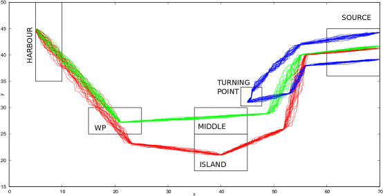
Figure 11: Passenger Travel Surveillance

We assume that we are given as predicates locations for way-points ships pass through or stop at along their route. In Fig. 11, predicates for way-points are marked with rectangles and labelled. Position information from 100 passengers is analyzed using PSI-Miner. It is known that a ship passes through at most five intermediate way-points. We, therefore, use a sequence length of $n=5$. On average, the time to move between way-points is known to be 70mins. We use a time delay of 70mins between events in the sequence. We examine using the target RISKY, representing passengers reported having the disease. We use predicates for way-points and the target. The following prefix sequences are learned:

ISLAND ##[0:140] !TURNING-POINT |-> ##[0:70] RISKY

Support = 17.63% Correlation = 52.5%

!ISLAND && MIDDLE ##[0:135.23] !TURNING-POINT |-> ##[0:70] !RISKY

Support = 7.53%, Correlation = 11.33%

From the prefixes learned, visiting the island has a 52% correlation with passengers marked risky (that are diagnosed with the disease). Those not visiting the island but passing through the middle are non-risky, with a correlation of 11.33%.

The predicate !TURNING-POINT is true for all positions other than within the rectangular region marked as TURNING-POINT, which is why it appears in all prefixes. However, we also want to know what happens to ships turning back? We explore further using the predicates TURNING-POINT and RISKY and learn the following prefixes:

TURNING-POINT |-> ##[0:70] !RISKY

Support = 18.98%, Correlation = 28.58%

In a time-series, for a risky (or non-risky) passenger, every time-position record is labelled as risky (or non-risky). Each prefix can explain (correlate with) only time-points after the prefix is satisfied, possibly a small portion of the time-series, that is labelled risky (or non-risky). Therefore the prefixes reported do not have a high correlation. Since, we never report a property unless it has 100% confidence, in this case, the correlation values are acceptable. The time-delay of ##[0:70] appears in the consequent of the PSI-L properties for the same reason.

From the mined properties, we learn that passengers visiting the island carry the disease, whereas passengers in ships turning around or passing through the middle region without visiting the island do not have disease symptoms. Authorities may then curtail visits to the island and inform travellers accordingly. ∎

Example 13.

A low-dropout voltage regulator (LDO), is a voltage regulator used to accurately maintain stable voltages for devices containing micro-electronics, such as processing units with varying power levels. During the design of the regulator, simulations produce behaviours that can be difficult to understand. We use PSI-Miner on the simulation of an LDO circuit to understand its operation. We use PSI-Miner to analyze the simulation depicted in Figure 12. Since the occurrence of a circuit event can span short periods of time, we use a low support threshold ($10^{-4}\%$). Time intervals in the prefixes are measured in seconds.

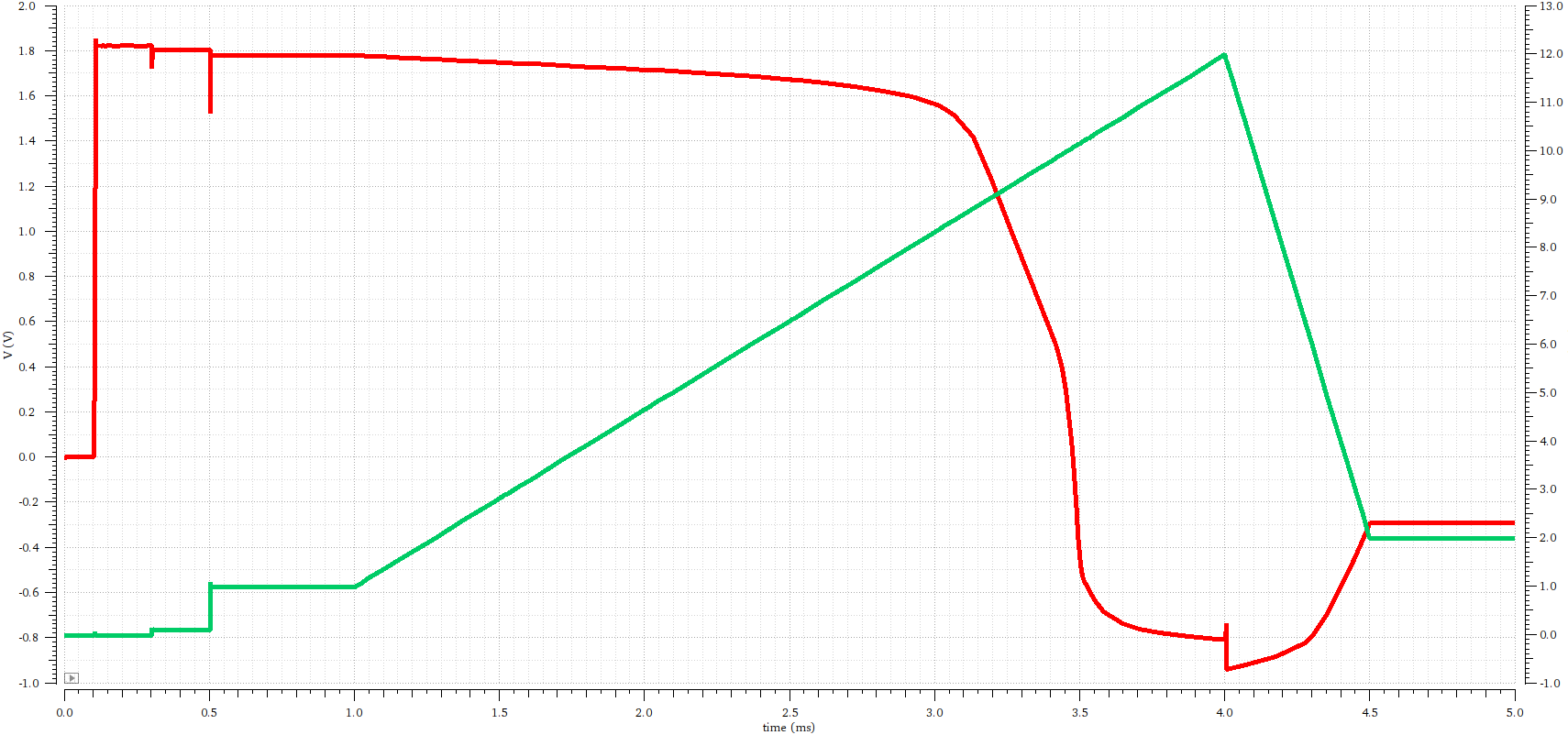
Figure 12: Waveform of voltage (volts) in red, and current (mA) in green, versus time (ms) depicting the behaviour of a low-dropout voltage regulator circuit.

The following are a selection of the properties that are mined:

“When at 10% of the rated voltage (VLowerBand: 0.18<=v<=0.19), while not in a state of short circuit (InShrtCkt: i>=0.0085), then sometime in the next 4.06$\mu s$ to 4.09$\mu s$ the terminal voltage rises to 90% of its rated value (VUpperBand: 1.62<=v<=1.63).”

!InShrtCkt && VLowerBand |-> ##[4.06e-06:4.09e-06] VUpperBand

(Support 0.0002%, Correlation: 0.023%)
The property has a very low correlation because the prefix containing the lower band (10%) crossing lasts for a very small amount of time. However, this property is significant, and provides insight into the rise-time of the LDO.

“When not in a state of short circuit, if the terminal voltage is at 90% of its rated value, then for some time between 0.4$\mu s$ to 0.63$\mu s$ it will not reach the rated value (VStable: 1.5<=v<=1.85).”

!InShrtCkt && VUpperBand |-> ##[ 4.0e-7:6.3e-7 ] !VStable

(Support: 1%, Correlation: 0.02%)
“When the short circuit event (ShrtCktEvent: 0.0085<=i<=0.009) isn’t in play, but the circuit is in a state of short circuit (current is above the 8.5mA threshold), then sometime in the next 20$\mu s$ the terminal voltage is not at its rated value.”

InShrtCkt && !ShrtCktEvent |-> ##[0.0:2.0e-05] !VStable

(Support: 23.19%, Correlation: 82.29%)
∎

Example 14.

A comparator suffers from a glitch that occurs on a digital port. We use PSI-Miner to mine correlations that may exist, looking for glitches that may have occurred on other lines within a short window of time. It is likely that if these occurred before the observed glitch on the digital port, they could have carried a disturbance across. PSI-Miner is provided with a list of Boolean expressions over a predicate alphabet (Table 2) and asked to explain the expression nrst1V8Band. The alias nrst1V8Band represents valid voltages for the digital port which may have been violated.

Predicate/Boolean Expression	Alias
nrst1V8 <= 0.05 || nrst1V8 >= 1.5	nrst1V8Band
uvlo<=0.0041 || uvlo>=0.740	uvloBand
ovlo<=0.0041 || ovlo>=1.5	ovloBand
enOsc <= 0.019	enOscBand
vreflow <=0.0270	vreflowBand
vrefhigh >=1.21	vrefhighBand
supptri<=0.00499	suppBand
clkrun<=-0.04	clkBand

Table 2: Predicate Alphabet used for PSI-Miner for the Comparator

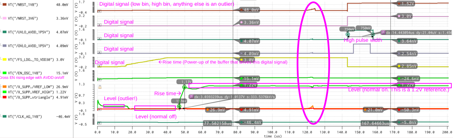
Figure 13: Glitch behaviour in an Comparator Circuit

“When the clock level and the UVLO are not within acceptable thresholds, and if within 6$\mu s$ the OVLO is also outside acceptable thresholds, then within 9$\mu s$ the nstr1V8Band also falls outside acceptable thresholds.”

!clkBand && !uvloBand ##[0.0:6.0e-06] !ovloBand |-> ##[0.0:9.0e-06] !nrst1V8Band

(Support: 3.01%, Correlation: 24.95%)
“When the clock and oscillator enable are not within acceptable thresholds and the UVLO is within its acceptable threshold, within the next 4.8$\mu s$ the nstr1V8Band falls outside acceptable thresholds.”

!clkBand && uvloBand && !enOscBand |-> ## [0.0:4.80e-06] !nrst1V8Band

(Support: 0.14%, Correlation: 12.85%)
The prefix sequences mined help identify that it is possible that the when the clkBand expression becomes false (there is jitter on the clock port), this leads to a cascading of jitters on other ports. In one case, the UVLO and OVLO both fall out of acceptable bands of operation, while in another the oscillator enable falls outside its acceptable band of operation. Such information may be useful in a root cause analysis and for monitoring for similar anomalies. ∎

PSI-Miner was able to compute the decision tree in under a second in our experiments. The computation time varies with the size of the interval set. The trend for CPU-Time as $n$ and $k$ vary is depicted in Figure 14. For every increasing incremental change in $n$, the number of pseudo-targets increases accordingly. This then increases the number of pseudo-targets against which unified gain is computed for every predicate. For a fixed predicate alphabet $\mathbb{P}$, for an increase in $n$ by one, a fixed number, $|\mathbb{P}|$, of new computations of unified gain are introduced. To demonstrate this, we use the data-set of the LDO of Example 13. We choose this example since this analog circuit has behaviours that occur in a scale of micro-seconds, while the trace itself is $5ms$ long, orders of magnitude longer than mined behaviours. We also use predicates having small truth intervals (a few micro-seconds long). In Figure 14, we record the CPU-Time to process the trace and generate the pseudo-targets (Input Processing), and to generate the decision tree (Tree Generation). Other constraints on the decision tree are the same as in Example 13.

We first vary $n$ in increments of 10, from 10 to 100, using a fixed delay resolution of $10^{-6}$ and use all the predicates from Example 13 as part of the predicate alphabet. We use the predicate VUpperBand as the target. We observe that as $n$ increases, the time to generate pseudo-targets varies around only marginally around $1.5ms$. On the other hand, we see a clear trend in the time to generate the decision tree. In general, we observe that the CPU-Time increases linearly with $n$.

Next, we vary $k$ in multiples of 2, starting with $k=10^{-6}$, while using a fixed prefix length of $n=10$, and all the predicates from Example 13. The target used is the same as earlier. We observe that as $k$ increases, the time to generate pseudo-targets varies marginally, around $1.5ms$, while in general the CPU-Time decreases with an increase in $k$. There seems to be no clear relationship between $k$ and CPU-time, beyond what is already stated. The decreasing trend of CPU-time with increasing values of $k$ is explained by the fact that although $k$ increases, the number of pseudo-targets remains constant. However, the number of truth intervals for the $i^{th}$ pseudo target may decrease. This is owed to the use of Minkowski difference with larger intervals, leading to the merging of truth intervals for the target. A decrease in the size of the interval set for a pseudo-target results in fewer set operations, resulting in a decrease in CPU-Time.

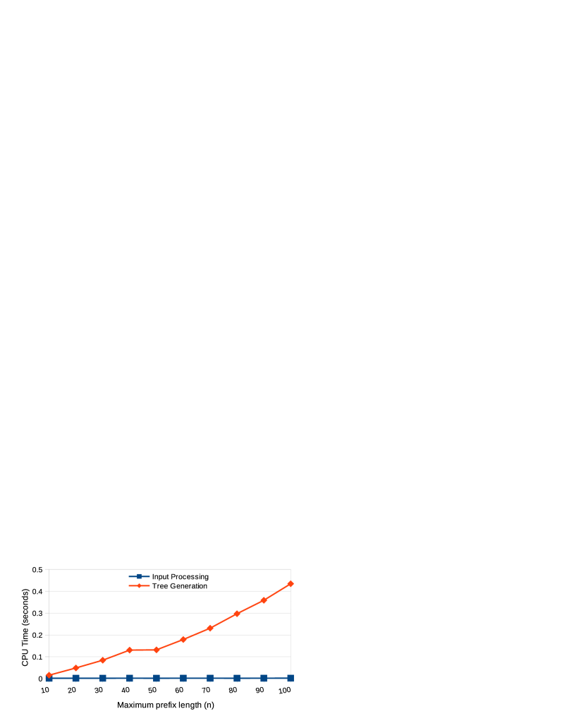
(a) CPU-Time versus prefix length (n)

(b) CPU-Time versus delay resolution (k)

Figure 14: CPU-Time for input processing and decision tree generation as $n$ and $k$ vary

9 Related Work

Mining information from time-series data has been a topic of study for decades (?, ?). Learning problems include but are not limited to the following:

1. Querying: Finding a time-series similar to a given one from a database. Methods include Singular Value Decomposition (SVD), Discrete Fourier transform (DFT), Discrete Wavelet Transforms (DWT) or Adaptive Piecewise Constant Approximations (APCA) and the dissimilarity metric to index the time-series (?, ?).

2. Clustering: Clustering time-series data using a similarity metric between time-series. For instance, in Debregeas & Hebrail, 1998, time-series recorded from the electrical power-grid are clustered together using Kohonen Maps, while in Kalpakis et al., 2001, distance measures are explored for clustering.

3. Summarization: Summarize a time-series with a representative approximation (?). Similarly, Van Wijk & Van Selow, 1999, discusses other methods for visualizing trends in a univariate time-series dataset.

4. Separation Features: Given time-series $\mathcal{S}$ and $\hat{\mathcal{S}}$, find interesting features that separate the two time-series. In Guralnik & Srivastava, 1999, time-series data is analyzed to determine interesting episodes in the time-series. In Keogh et al., 2002,the authors suggest discretizing the time-series and finding sub-strings that occur most frequently in the time-series.

5. Prediction: Given a time-series $\mathcal{S}$ over time points $(t_{1},...,t_{n})$, predict the behaviour of $\mathcal{S}$ as if observed over time points $(t_{n+1},...,t_{n+k})$. Studies in this area have been reported in Brockwell & Davis, 2002; Harris & Sollis, 2003; Tsay, 2005; and Brockwell & Davis, 1986.

6. Anomaly detection: The problem of detecting a pattern that deviates from a nominal behaviour is strongly linked to the problem of prediction. Like prediction, it also relies on having a sufficiently accurate model of the time-series to be able to identify deviations (?, ?, ?).

7. Motif Discovery: A sub-sequence that is observed frequently in a time-series is called a Motif. A detailed review of existing literature in this area can be found in Esling & Agon, 2012.

These approaches do not address the problem considered in this paper, namely to find causal sequences of predicates that explain a given consequent. More recently, the focus of learning has been to learn artifacts about time-series that can be expressed in logic and are therefore inherently explainable. These studies are broadly broken down into the following two types:

• Learning properties from templates: A template property is provided. The learning problem is to choose property parameter values that best represent the time-series.

• Learning property structure and parameter values: Given a syntax for the property, learn the property that best represents the time-series.

We summarize related work in these problems and position our work against them.

9.1 Learning from Templates

A large repository of work exists on mining parameter values for a template property in parametric STL (PSTL) (?, ?, ?, ?) with the aim of optimizing property robustness for the given time-series trace. The work in Asarin et al., 2012, proposes learning the range of valid parameter values for a PSTL property that a given set of dense-time real-valued system traces satisfy. Given a formula in PSTL, the authors of Asarin et al., 2012, and Bakhirkin et al., 2018, propose techniques to compute a validity domain for the formula’s time and value parameters such that all traces satisfy the formula given these domains. In Yang et al., 2012, the authors propose a methodology to compute parameter domains for a property in MTL that a given embedded and hybrid system satisfies.

In Jin et al., 2015, the authors propose learning parameter values that satisfy system requirements expressed as template properties in PSTL. They iterate on the domain of parameter values until they converge on a combination of values that make the property valid for the given set of traces.

Methods for template-based learning require a parameterized property expressed in a formal logic such as MTL or STL. This means that the predicates that influence a given consequent are known, and the parameter values are learned. The learning problem is thereby transformed into a parameter optimization problem. Some of these works also assume the existence of a model of the system.

These methods are not applicable to cases where nothing is known about the factors that influence the truth of a given consequent, yet we wish to find the causal sequence of events. Our contribution is in providing a methodology that learns the timed sequence of predicates that cause the consequent, which involves learning the relevant predicates, as well as the real-time timing between them.

9.2 Learning Property Structure and Parameter Values

While in Section 9.1 a formula structure was provided as input to the learning task, we now summarize property mining studies in which such templates are not-provided.

The work on Temporal Logic Inference (TLI) in Kong et al., 2014, aims to classify two labelled sets of time-series by learning distinguishing Boolean combinations of temporal properties of the form $F_{[t_{1},t_{2})}\psi$ or $G_{[t_{1},t_{2}]}\psi$, where $\psi$ is Boolean. The work in Bombara et al., 2016, improves the methodology in Kong et al., 2014, to allow for multiple predicates in the antecedent and properties of the form $F_{[t_{1},t_{2})}\varphi_{g}$ or $G_{[t_{1},t_{2}]}\varphi_{f}$. The predicate and timing constants are learned using local search heuristic algorithms like simulated annealing, while the property structure is learned using standard decision trees. As we have shown in our work, using standard decision trees for learning temporal logic properties can lead to misleading outcomes. Moreover, the methodologies of Kong et al., 2014 and Bombara et al., 2016, do not address our problem of finding a causal sequence for a given consequent. One straightforward way of adapting their work is to perform a splitting of traces into two classes of sub-traces of length $n\times k$, one class containing $E$ and the other containing $\neg E$. Note that in both types of traces, it is possible that there exist both, time-points where $E$ is true and others where $\neg E$ is true. Hence, in both sets there would be similar event sequences, with similar delays between events, associated differently with $E$ and $\neg E$. This could result in an empty or misleading outcome. On the other hand, the work proposed here could be adapted to work with classification problems. One way to achieve this is to introduce an variable denoting class type with appropriate values at all time-points in all traces. For instance, consider trace sets $\mathbb{T}_{A}$ and $\mathbb{T}_{B}$ containing traces of two classes $A$ and $B$. Introduce a new variable $"class"$, with $class==A$ true at all time-points of traces of class $A$, and false for all time-points of traces of class $B$. We now use the proposed PSI-Miner methodology to mine properties with $E\equiv class==A$ as the target. We successfully used this technique in Example 12 to identify key differences between passenger movements labeled RISKY and !NON-RISKY.

The work in Bartocci et al., 2014, learns a discriminator property to distinguish between traces generated by two different processes. The method relies on using a statistical abstraction of the data in the traces. The property structure and parameters are optimized separately.

Past work in Yang & Evans, 2004; Yang et al., 2006; Gabel & Su, 2008a, 2008b; and De-Orio et al., 2009, focuses on mining sequences and causal relations for program events. The most recent study examines program traces and learns a finite automaton, over a user-defined alphabet, describing all the ways (up to a discrete event bound on path length) of violating a propositional assertion given in the program (?). Older studies focus on mining cause-effect relations in programs as LTL properties (?, ?, ?, ?). The methodology in Cutulencoet al., 2016, mines timed regular expressions from program traces, while in Garg et al.,2016, decision trees are used to learn invariants for software programs. In these works, the sequences mined do not preserve timing information between the events.

The tool Goldmine (?) uses decision trees to mine causal relations from clocked traces of Boolean systems as an ordering of events. The assertions mined are in a subset of LTL limited to bounded safety and liveness. The work in Kauffman & Fis-chmeister, 2017, mines Allen’s interval relations, specifically event intervals from clocked event traces. The proposed methodology mines nfer rules (based on Allen’s Temporal Logic) from learned before relations given a set of clocked event traces. The learned sequences are a series of before relations between events in the traces. These techniques are not applicable to real-time data from dense-time systems.

To the best of our knowledge, ours is the first work on mining sequences consisting of Boolean combinations of predicates over real variables separated by dense real time delay intervals that causally determine the truth of a given consequent. Our methodology automatically finds the predicate combinations that influence the consequent as well as the real time delay intervals that separate them. Although we start with a property skeleton consisting of bucket positions and template delay intervals, the learning methodology automatically fills the buckets by choosing relevant predicates, merges empty buckets, and tightens the delays between the buckets to return dense time temporal properties for explaining the truth of the consequent.

10 Conclusions

In complex dynamical systems, the task of finding the causal trigger of an event is an important and non-trivial task. The AI/ML community seeks data-driven solutions for such problems. Our approach of mining prefix sequences addresses this task. Prefix sequences expressed in logic are easily readable and are easy to explain.

Properties mined using our methodology are useful in many different contexts. This includes the following:

1. Anomaly Detection. Anomalies may be viewed as deviations from set patterns in the data. If a property mined from legacy data fails during the execution of the system, then it may be an anomaly. Properties can be readily monitored over simulation and real-time execution, and can thereby be used to detect anomalies.

2. Prediction. The mined properties can be monitored at runtime to predict future events. For example, when the prefix-sequence at the antecedent of a property matches the runtime behavior, the consequent can be predicted within the corresponding delay interval.

3. Clustering. Time-series data can be partitioned into clusters on the basis of the truth of the mined properties. Also, for a given consequent we may have mined different prefix-sequences. Clustering the data based on the matches of the prefix-sequence help us to separate out data corresponding to different causes that lead to the same outcome.

There are several interesting offshoots from our work. For example:

• Incorporating domain knowledge. If we already know some properties over the variables in the system, then the mining algorithm can be suitably modified to ensure that the mined properties do not contradict the domain knowledge. This is particularly necessary for safety-critical systems, where corner case safety properties are not well represented in the data.

• Finding separation features. Separation features are properties that explain the difference between two sets of time-series data sets. To facilitate the readability of the differences, we need to mine properties over similar predicates and having similar structure. This requires considerable modification in the mining algorithm and is one of the future directions being pursued by us.

• Mining properties with recurrent behaviors. Suppose a consequent event, $E$, is caused when a predicate $P$ remains true for more than 20 seconds. Such a property cannot be mined using the present approach because the recurrent requirement for predicate $P$ cannot be captured in the present language. This is also an interesting direction of our future research.

We believe that there are many other possible directions of research based on the contributions of this paper. The increasing significance of finding causal sequences in data driven learning approaches adds to the impact potential of the methods presented in this paper.

References

- Aggarwal Aggarwal, C. C. (2015). Data Mining: The Textbook. Springer Publishing Company, Incorporated.
- Asarin et al. Asarin, E., et al. (2012). Parametric identification of temporal properties. In Proc. of the 2nd International Conference on Runtime Verification, pp. 147–160.
- Bakhirkin et al. Bakhirkin, A., et al. (2018). Efficient parametric identification for stl. In HSCC, HSCC ’18, pp. 177–186. ACM.
- Chakrabarti et al. Chakrabarti, K., et al. (2002). Locally adaptive dimensionality reduction for indexing large time series databases. ACM Trans. Database Syst., 27(2), 188–228.
- Chang & Wang Chang, P. H., & Wang, L. C. (2010). Automatic assertion extraction via sequential data mining of simulation traces. In ASP-DAC, pp. 607–612.
- Chockler et al. Chockler, H., et al. (2020). Learning the language of software errors. J. Artif. Intell. Res., 67, 881–903.
- Danese et al. Danese, A., et al. (2015a). Automatic extraction of assertions from execution traces of behavioural models. In Proc. of DATE, pp. 67–72.
- Danese et al. Danese, A., et al. (2015b). A time-window based approach for dynamic assertions mining on control signals. In Proc. of VLSI-SoC, pp. 246–251.
- Esling & Agon Esling, P., & Agon, C. (2012). Time-series data mining. ACM Comput. Surv., 45(1), 12:1–12:34.
- Evans & Grefenstette Evans, R., & Grefenstette, E. (2018). Learning explanatory rules from noisy data. J. Artif. Int. Res., 61(1), 1–64.
- Faloutsos et al. Faloutsos, C., et al. (1994). Fast subsequence matching in time-series databases. In Proceedings of the 1994 ACM SIGMOD International Conference on Management of Data, SIGMOD ’94, pp. 419–429. ACM.
- Guo et al. Guo, R., et al. (2018). A survey of learning causality with data: Problems and methods. CoRR, abs/1809.09337.
- IEEE IEEE (2010). 1850-2010 - IEEE Standard for Property Specification Language (PSL) (https://standards.ieee.org/findstds/standard/1850-2010.html)..
- IEEE IEEE (2012). 1800-2012 - IEEE Standard for SystemVerilog–Unified Hardware Design, Specification, and Verification Language(http://standards.ieee.org/findstds/standard/1800-2012.html)..
- Indyk et al. Indyk, P., et al. (2000). Identifying representative trends in massive time series data sets using sketches. In Proceedings of the 26th International Conference on Very Large Data Bases, VLDB ’00, pp. 363–372, San Francisco, CA, USA. Morgan Kaufmann Publishers Inc.
- J. R. Quinlan J. R. Quinlan (1993). C4.5: Programs for Machine Learning. Morgan Kaufmann Publishers Inc., San Francisco, CA, USA.
- Jin et al. Jin, X., et al. (2015). Mining requirements from closed-loop control models. IEEE Transactions on Computer Aided Design of Integrated Circuits and Systems, 34(11), 1704–1717.
- Lemieux et al. Lemieux, C., et al. (2015). General ltl specification mining (t). In Proc. of ASE.
- Ma & Perkins Ma, J., & Perkins, S. (2003). Online novelty detection on temporal sequences. In Proceedings of the Ninth ACM SIGKDD International Conference on Knowledge Discovery and Data Mining, KDD ’03, pp. 613–618, New York, NY, USA. ACM.
- Maler & Nickovic Maler, O., & Nickovic, D. (2004). Monitoring temporal properties of continuous signals. In Proceedings of Formal Modeling and Analysis of Timed Systems (FORMATS-FTRTFT). Volume 3253 of LNCS, pp. 152–166. Springer.
- Mitchell Mitchell, T. M. (1997). Machine Learning (1 edition). McGraw-Hill, Inc., New York, NY, USA.
- Ott & Longnecker Ott, R. L., & Longnecker, M. T. (2006). Introduction to Statistical Methods and Data Analysis (with CD-ROM). Duxbury Press, Boston, MA, USA.
- Pearl Pearl, J. (1995). Causal diagrams for empirical research. Biometrika, 82(4), 669–688.
- Pearl Pearl, J. (2000). Causality: Models, Reasoning, and Inference. Cambridge University Press, New York, NY, USA.
- Pearl Pearl, J. (2019). The seven tools of causal inference, with reflections on machine learning. Commun. ACM, 62(3), 54–60.
- Pearl et al. Pearl, J., et al. (2009). Causal inference in statistics: An overview. Statistics surveys, 3, 96–146.
- Pnueli Pnueli, A. (1977). The temporal logic of programs. In Proceedings of the 18th Annual Symposium on Foundations of Computer Science, SFCS ’77, pp. 46–57, Washington, DC, USA. IEEE Computer Society.
- Quinlan Quinlan, J. R. (1986). Induction of decision trees. Mach. Learn., 1(1), 81–106.
- Ralanamahatana et al. Ralanamahatana, C. A., et al. (2005). Mining Time Series Data, pp. 1069–1103. Springer US.
- Vasudevan et al. Vasudevan, S., et al. (2010). GoldMine: Automatic assertion generation using data mining and static analysis. In Proc. of DATE, pp. 626–629.
- Yang et al. Yang, H., et al. (2012). Querying parametric temporal logic properties on embedded systems. In Prof. of ICTSS.
- Ypma et al. Ypma, A., et al. (1997). Novelty detection using self-organizing maps. In In Proc. of ICONIP’97, pp. 1322–1325. Springer.
- Zhong & Khoshgoftaar Zhong, S., & Khoshgoftaar, T. M. (2007). Clustering-based network intrusion detection. International Journal of Reliability, Quality and Safety Engineering, 14(2), 169–187.