Instant Quantization of Neural Networks using Monte Carlo Methods

Abstract

Low bit-width integer weights and activations are very important for efficient inference, especially with respect to lower power consumption. We propose to apply Monte Carlo methods and importance sampling to sparsify and quantize pre-trained neural networks without any retraining. We obtain sparse, low bit-width integer representations that approximate the full precision weights and activations. The precision, sparsity, and complexity are easily configurable by the amount of sampling performed. Our approach, called Monte Carlo Quantization (MCQ), is linear in both time and space, while the resulting quantized sparse networks show minimal accuracy loss compared to the original full-precision networks. Our method either outperforms or achieves results competitive with methods that do require additional training on a variety of challenging tasks.

1 Introduction

Developing novel ways of increasing the efficiency of neural networks is of great importance due to their widespread usage in today’s variety of applications. Reducing the network’s footprint enables local processing on personal devices without the need for cloud services. In addition, such methods allow for reducing power consumption - also in data centers. Very compact models can be fully stored and executed on-chip in specialized hardware like for example ASICs or FPGAs. This reduces latency, increases inference speed, improves privacy concerns, and limits bandwidth cost.

Quantization methods usually require re-training of the quantized model to achieve competitive results. This leads to an additional cost and complexity. The proposed method, Monte Carlo Quantization (MCQ), aims to avoid retraining by approximating the full-precision weight and activation distributions using importance sampling. The resulting quantized networks achieve close to the full-precision accuracy without any kind of additional training. Importantly, the complexity of the resulting networks is proportional to the number of samples taken.

First, our algorithm normalizes the weights and activations of a given layer to treat them as probability distributions. Then, we randomly sample from the corresponding cumulative distributions and count the number of hits for every weight and activation. Finally, we quantize the weights and activations by their integer count values, which form a discrete approximation of the original continuous values. Since the quality of this approximation relies entirely on (quasi)random sampling, the accuracy of the quantized model is directly dependent on the amount of sampling performed. Thus, accuracy may be traded for higher sparsity and speed by adjusting the number of samples. On the challenging tasks of image classification, language modeling, speech recognition, and machine translation, our method outperforms or is competitive with existing quantization methods that do require additional training.

2 Related Work

The computational cost of neural networks can be reduced by pruning redundant weights or neurons, which has been shown to work well [8, 22, 12]. Alternatively, the precision of the network weights and activations may be lowered, potentially introducing sparsity. Using low precision computations to reduce the cost and sparsity to skip computations allows for efficient hardware implementations [16, 36]. This is the approach used in this paper.

BinaryConnect  [4] proposed training with binary weights, while XNOR-Net  [28] and BNN  [10] extended this binarization to activations as well. TWN  [15] proposed ternary quantization instead, increasing model expressiveness. Similarly, TTQ  [44] used ternary weights with a positive and negative scaling learned during training. LR-Net  [32] made use of both binary and ternary weights by using stochastic parameterization while INQ  [42] constrained weights to powers of two and zero. FGQ  [19] categorized weights in different groups and used different scaling factors to minimize the element-wise distance between full and low-precision weights. [38] used the hardware accelerator’s feedback to perform hardware-aware quantization using reinforcement learning. [40] jointly trained quantized networks and respective quantizers. [29] used Bloomier filters to compactly encode network weights.

Similarly, quantization techniques can also be applied in the backward pass. Therefore, some previous work quantized not only weights and activations but also the gradients to augment training performance  [43, 7, 3]. In particular, RQ  [17] propose a differentiable quantization procedure to allow for gradient-based optimization using discrete values and  [39] recently proposed to discretize weights, activations, gradients, and errors both at training and inference time.

These quantization techniques have great benefits and have shown to successfully reduce the computation requirements compared to full-precision models. However, all the aforementioned methods require re-training of the quantized network to achieve close to full-precision accuracy, which can introduce significant financial and environmental cost [34]. On the other hand, our method instantly quantizes pre-trained neural networks with minimal accuracy loss as compared to their full-precision counterparts without any kind of additional training.

3 Neural Networks and Monte Carlo Methods

Neural networks make extensive use of randomization and random sampling techniques. Examples are random initialization of network weights, stochastic gradient descent [30], regularization techniques such as Dropout [33] and DropConnect [37], data augmentation and data shuffling, recurrent neural networks’ regularization [20], or the generator’s noise input on generative adversarial networks [6].

Many state-of-the-art networks use ReLU [24], which has interesting properties such as scale-invariance. This enables a scaling factor to be propagated through all network layers without affecting the network’s original output. This principle can be used to normalize network values, such as weights and activations, as further described in Section 3.1. After normalization, these values can be treated as probabilities, which enables the simulation of discrete probability densities to approximate the corresponding full-precision, continuous distributions (Section 3.2).

3.1 Network Normalization

Assuming the exclusive use of the ReLU activation function in the hidden layers, the scale-invariance property of the ReLU activation function allows for arbitrary scaling of the weights or activations without affecting the network’s output. Given weights $w_{l-1,i,j}$ connecting the $i$-th neuron in layer $l-1$ to the $j$-th neuron in layer $l$, where $i\in\left[0,N_{l-1}-1\right]$ and $j\in\left[0,N_{l}-1\right]$, with $N_{l-1}$ and $N_{l}$ the number of neurons of layer $l-1$ and $l$, respectively. Let $a_{l,j}$ be the $j$-th activation in the $l$-th layer and $f\in\mathbb{R}^{+}$: $a_{l,j}=max\Bigg{\{}0,\sum_{i=0}^{N_{l-1}-1}w_{l-1,i,j}a_{l-1,i}+b_{l,j}\Bigg{\}}=f\cdot max\Bigg{\{}0,\frac{\sum_{i=0}^{N_{l-1}-1}w_{l-1,i,j}a_{l-1,i}+b_{l,j}}{f}\Bigg{\}}.$

Biases and incoming weights for neuron $j$ in layer $l$ may then be normalized by $f=\|\mathbf{w}_{l-1,j}\|_{1}=\sum_{i=0}^{N_{l-1}-1}|w_{l-1,i,j}|$,

enabling weights to be seen as a probability distribution over all connections to a neuron. A similar procedure could be used to normalize all activations $a_{l,j}$ of layer $l$.

Propagating these scaling factors forward layer by layer results in a single scalar (per output), which converts the outputs of the normalized network to the same range as the original network. This technique allows for the usage of integer weights and activations throughout the entire network without requiring rescaling or conversion to floating point at every layer.

3.2 Network Quantization

Taking advantage of the normalized network, we can simulate discrete probability densities by constructing a probability density function (PDF) and then sampling from the corresponding cumulative density function (CDF). The number of references of a weight is then the quantized integer approximation of the continuous value. For simplicity, the following discussion shows the quantization procedure for weights; activations can be quantized in the same way at inference time.

Without loss of generality, given $n$ weights, assuming $\sum_{k=0}^{n-1}|w_{k}|=\|w\|_{1}=1$ and defining a partition of the unit interval by $P_{m}:=\sum_{k=1}^{m}|w_{k}|$ we have the following partitions:

(1)

Then, given $N$ uniformly distributed samples $x_{i}\in[0,1)$, we can approximate the weight distribution as follows:

$$\sum_{j=0}^{n-1}w_{j}a_{j}\approx\frac{1}{N}\sum_{i=0}^{N-1}\underbrace{\text{sign}(w_{j_{i}})}_{\in\{-1,0,1\}}\times a_{j_{i}},$$ (2)

where $j_{i}\in\{0,\ldots,n-1\}$ is uniquely determined by $P_{j_{i}-1}\leq x_{i}<P_{j_{i}}$.

One can further improve this sampling process by using jittered equidistant sampling. Thus, given a random variable $\xi\in[0,1)$, we generate N uniformly distributed samples $x_{i}\in[0,1)$ such that $x_{i}=\dfrac{i+\xi}{N}$, where $i\in\{0,\ldots,N-1\}$. The combination of equidistant samples and a random offset improves the weight approximation, as the samples are more uniformly distributed. The variance of different sampling seeds is discussed in the Appendix.

4 Monte Carlo Quantization (MCQ)

Our approach builds on the aforementioned ideas of network normalization and quantization using random sampling to quantize an entire pre-trained full-precision neural network. As before, we focus on weight quantization; online activation quantization is discussed in Section 4.4. Our method, called Monte Carlo Quantization (MCQ), consists of the following steps, which are executed layer by layer:

1. Create a probability density function (PDF) for all $N_{l,w}$ weights of layer $l$ such that $\sum_{i=0}^{N_{l,w}-1}|w_{l,i}|=1$ (Section 4.1).

2. Perform importance sampling on the weights based on their magnitude by sampling from the corresponding cumulative density function (CDF) and counting the number of hits per weight (Section 4.2).

3. Replace each weight with its quantized integer value, i.e. its hit count, to obtain a low bit-width, integer weight representation (Section 4.3).

The pseudo-code for our method is shown in Algorithm 1 of the Appendix. Figure 1 illustrates both the normalization and importance sampling processes for a layer with 10 weights and 1 sample per weight, i.e. $K=1.0$.

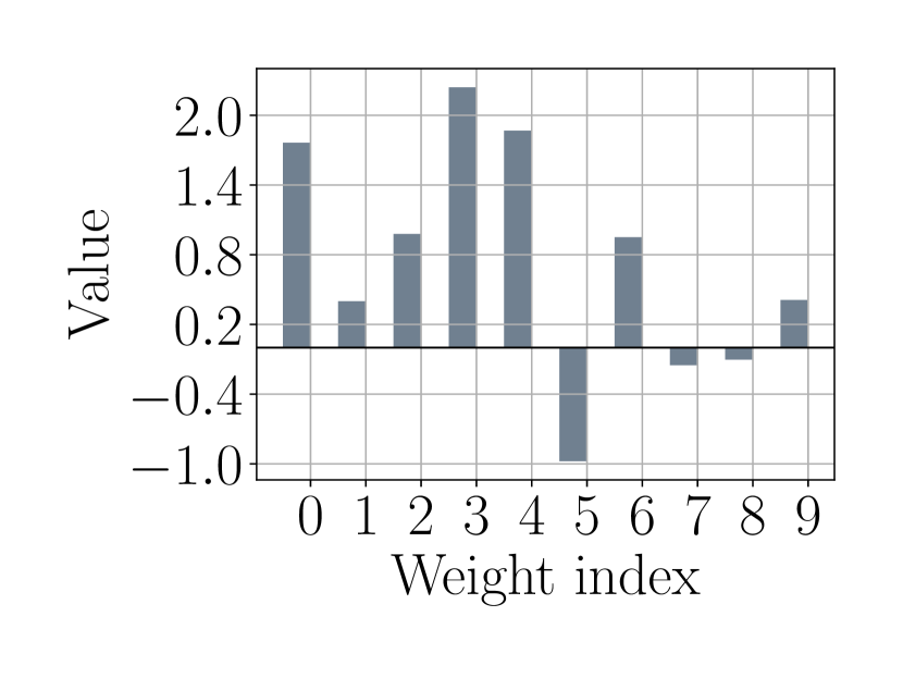
(a) Full-precision weights

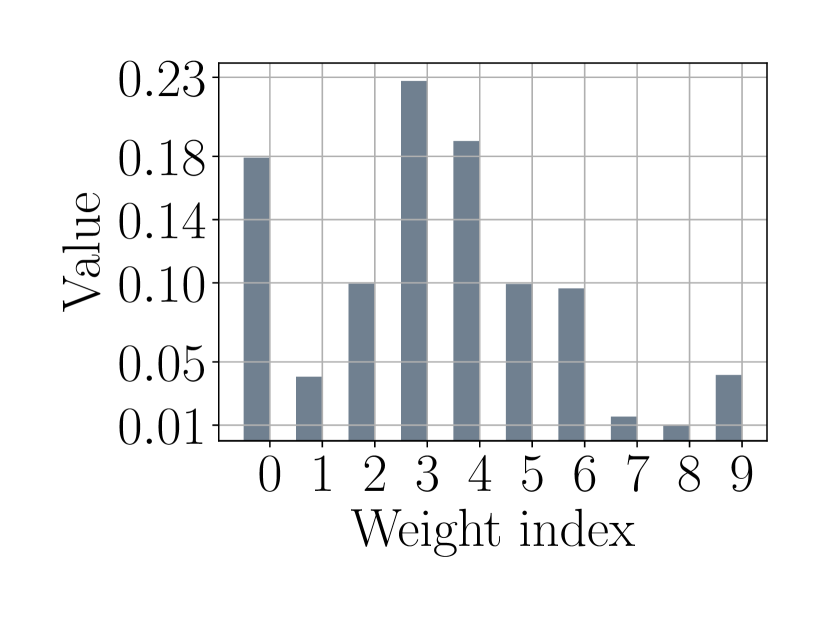
(b) PDF

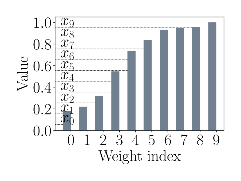
(c) Sampling on CDF

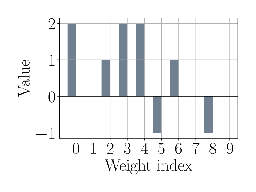
(d) Integer weights

Figure 1: Starting from full-precision weights (a), we create a PDF of the sorted absolute values (b) and uniformly sample from the corresponding CDF (c). The sampling process produces quantized integer network weights based on the number of hits per weight (d). Note that since weights 7, 8, and 9 were not hit, sparsity is introduced which can be exploited by hardware accelerators.

4.1 Layer Normalization

Performing normalization neuron-wise, as introduced in Section 3.1 may result in an inferior approximation, especially when the number of weights to sample from is small, as for example in convolutional layers with a small number of filters or input channels. To mitigate this, we propose to normalize all neurons simultaneously in a layer-wise manner. This has the additional advantage that samples can be redistributed from low-importance neurons to high-importance neurons (according to some metric), resulting in an increased level of sparsity. Additionally, there is more opportunity for global optimization, so the overall weight distribution approximation improves as well.

We use the 1-norm of all weights of a given layer $l$ as the scaling factor $f$ used to perform weight normalization. Thus, each normalized weight can be seen as a probability with respect to all connections between layer $l-1$ and layer $l$, instead of a single neuron. This layer-wise normalization technique is similar to Weight Normalization [31], which decouples the neuron weight vector magnitude from its direction.

4.2 Importance Sampling

As introduced in Section 3.2, we generate ternary samples (hit positive weight, hit negative weight, or no hit), and count such hits during the sampling process. Note that even though the individual samples are ternary, the final quantized values may not be, because a single weight can be sampled multiple times. We use jittered equidistant (stratified) sampling, to ensure uniform distribution. Given a random variable $\xi\in[0,1)$, we generate N samples $x_{i}\in[0,1)$ such that $x_{i}=\dfrac{i+\xi}{N}$, where $i\in\{0,\ldots,N-1\}$. This stratified sampling strategy also reduces the cost of the sampling process from $\mathcal{O}(NlogN)$ to $\mathcal{O}(N)$, as searching for the value corresponding to a sample does requires a binary search as it would for fully random sampling. The number of samples $N=K\cdot N_{values}$, where $K\in\mathbb{R}^{+}$ is a user-specified parameter to control the number of samples and $N_{values}$ represents the number of weights of a given layer. By varying K, the computational cost of sampling can be traded off better approximation (more bits per weight) of the original weight distribution, leading to higher accuracy. In our experiments, $K$ is set the same for all network layers.

One simple modification to enhance the quality of the discrete approximation is to sort the continuous values prior to creating the PDF. Applying sorting mechanisms to Monte Carlo schemes has been shown to be beneficial in the past [13, 14]. Sorting groups smaller values together in the overall distribution. Since we are using a uniform sampling strategy, smaller weights are then sampled less often, which results in both higher sparsity and a better quantized approximation of the larger weights in practice. This effect is particularly significant on smaller layers with fewer weights.

Since the quantized integer weights span a different range of values than the original weights, and biases remain unchanged, care must be taken to ensure the activations of each neuron are calculated correctly. After the integer multiply-accumulate (MAC) operation, the result must then be scaled by $\frac{f}{N}$ before adding the bias. This requires the storage of one floating point scaling value per layer. However, weights are stored as low bit-width integers and the computational cost is greatly reduced since the MAC operations use low-precision integers only instead of floating point numbers.

4.3 Layer Quantization

The number of bits required for the weights $B_{W_{l}}\in\mathbb{N}$, for layer $l$ and its quantized weights $Q(w_{l,i})$, corresponds to the bit amount needed to represent the highest hit count during sampling, including its sign: $B_{W_{l}}=1+\left\lfloor\log_{2}\left(\max_{0\leq i\leq N_{w}-1}|Q(w_{l,i})|\right)\right\rfloor+1$. Alternatively, positive and negative weights could be separated into two sets.

4.4 Online Quantization

While weights are quantized offline, i.e. after training and before inference, activations are quantized online during inference time using the same procedure as weight quantization previously described. Thus, in the normalization step (Section 4.1), all $N_{l,a}$ activations of a given layer $l$ are treated as a probability distribution over the output features, such that $\sum_{j=0}^{N_{l,a}-1}|a_{l,j}|=1$. Then, in the importance sampling step (Section 4.2), activations are sub-sampled using possibly different relative sampling amounts, i.e. $K$, than the ones used for the weights (we use the same $K$ for both weights and activations in all of our experiments). The required number of bits $B_{A_{l}}$ for the quantized activations $Q(a_{l,j})$ can also be calculated similarly as described in Section 4.3, although no additional bit sign is required when using ReLU since all activations are non-negative.

5 Experiments

The proposed method is extensively evaluated on a variety of tasks: for image classification we use CIFAR-10 [11], SVHN [25], and ImageNet [5], on multiple models each. We further evaluate MCQ on language modeling, speech recognition, and machine translation, to assess the preformance of MCQ across different task domains.

Due to the automatic quantization done by MCQ, some layers may be quantized to lower or higher levels than others. We indicate the quantization level for the whole network by the average number of bits, e.g. ’8w-32a’ means that on average 8 bits were used for weights and 32 bits for activations on each layer.

Many works note that quantizing the first or last network layer reduces accuracy significantly [8, 43, 15]. We use footnotes , , and to denote the special treatment of first or last layers respectively. For MCQ we report the results with both quantized and full-precision first layer. We do not quantize Batch Normalization layers as the parameters are fixed after training and can be incorporated into the weights and biases [39].

Tables 1, 2, 3 and 4 show the accuracy difference $\Delta$ between the quantized and full-precision models. For other compared works this difference is calculated using the baseline models reported in each of the respective works. We didn’t perform any search over random sampling seeds for MCQ’s results.

5.1 CIFAR-10

The best accuracies on VGG-7, VGG-14, and ResNet-20 produced by our method using $K=1.0$ on CIFAR-10 are shown in Table 1. We refer to the Appendix for model and training details. MCQ outperforms or shows competitive results showing minimal accuracy loss on all tested models against the compared methods that require network re-training. The full-precision baselines for BNN [10] and XNOR-Net [28] are from BC [4] as these works use the same model. Similarly, BWN [28]’s results on VGG-7 are the ones reported in TWN [15] since they did not report the baseline in the original paper.

Figure 2 shows the effects of varying the amount of sampling, i.e. using $K\in\left[0.1...2.0\right]$. The average percentage of used weights/activations per layer and corresponding bit-widths of the final quantized model is also presented on each graph. We observe a rapid increase of the accuracy even when sparsity levels are high on all tested models.

Table 1: Accuracy results on CIFAR-10 when quantizing either weights or activations or both. Quantizing only the weights leads to an accuracy loss of $\approx 1.0\%$ in the worst case. Quantizing both weights and activations does not reduce accuracy on VGG-7 while ResNet-20’s accuracy decreases by $\approx 1.0\%$. Quantizing the first layer results in an additional $\approx 0.5\%$ accuracy loss on all models.

Method VGG-7 VGG-14 ResNet-20 Full Precision (32w-32a) 91.23 92.49 95.02 $\Delta$ MCQ (quantized w) -0.48 (6.1w-32a) / +0.041 (6.1w-32a) -1.04 (6.7w-32a) / -0.501 (6.8w-32a) -0.84 (5.1w-32a) / -0.541 (5.1w-32a) $\Delta$ MCQ (quantized a) -0.121 (32w-5.68a) -0.061(32w-5.51a) -0.281(32w-6.3a) $\Delta$ MCQ (quantized w + a) -0.58 (6.1w-5.6a) / -0.131 (6.1w-5.6a) -1.08 (6.6w-5.3a) / -0.541 (6.8w-5.5a) -1.77 (5.1w-5.3a) / -1.211 (5.1w-5.3a) $\Delta$ TTQ (2w-32a) - - -0.641 $\Delta$ dLAC (2w-32a) - -3.0 / -1.41 - $\Delta$ TWNs (2w-32a) -0.06 - - $\Delta$ BC (1w-32a) +0.74 - - $\Delta$ BNN (1w-1a) +0.491 - - $\Delta$ BWN (1w-32a) -0.36 / +0.761 - - $\Delta$ XNOR-Net (1w-1a) +0.471 - - $\Delta$ RQ (8w-8a)) +0.25 - - $\Delta$ LR-net (2w-32a) -0.112 - -

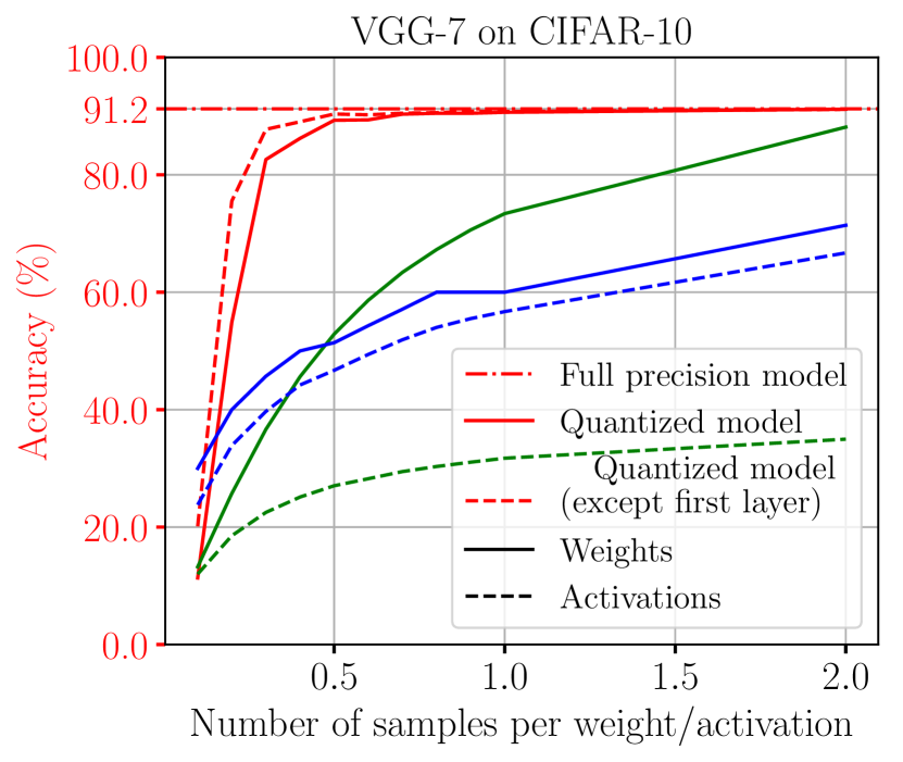
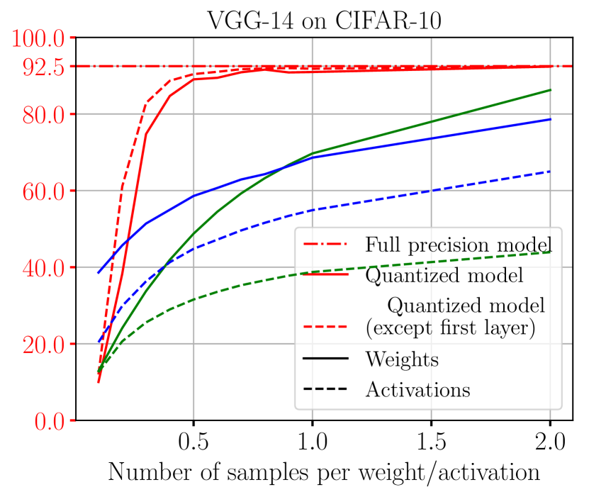
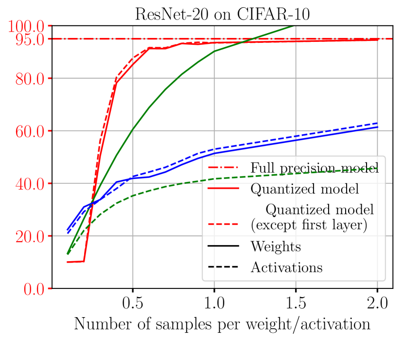
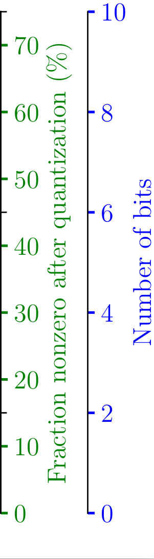
Figure 2: Results of quantizing both weights and activations on CIFAR-10 using different sampling amounts. The quantized models reach close to full-precision accuracy at around half the sample size while using only around half the weights and one-third of the activations of the full-precision models.

5.2 SVHN

For SVHN, the tested models are identical to the compared methods. Models B, C, and D have the same architecture as Model A but with a 50%, 75%, and 87.5% reduction in the number of filters in each convolutional layer, respectively [43]. We refer to the Appendix for further details.

Table 2 shows MCQ’s results for several models on SVHN using $K=1.0$. On bigger models, i.e. VGG-7* and Model A, we see minimal accuracy loss when compared to the full-precision baselines. For the smaller models, we observe a slight accuracy degradation as model size decreases due to the reduction in the sample size, resulting in a poorer approximation. However, we used only about 4 bits per weight/activation for such models. Thus, increasing the number of samples would improve accuracy while still maintaining a low bit-width. Figure 3 illustrates the consequences of varying the number of samples. Less samples are required than on CIFAR-10 for bigger models to achieve close to full-precision accuracy. Potentially this is because layers have a larger number of weights and activations, so a larger sample size reduces quantization noise since the important values being more likely to be better approximated.

Table 2: Accuracy results on SVHN when quantizing weights, activations, or both. On VGG-7*, MCQ shows minimal accuracy loss when quantizing both weights and activations and close to no accuracy loss when not quantizing the first layer. For models A, B, C, and D the accuracy lowers as the model size decreases. Quantizing only the activations barely lowers the baseline accuracy.

Method VGG-7* Model A Model B Model C Model D Full Precision (32w-32a) 94.06 96.01 95.03 94.08 91.08 $\Delta$ MCQ (quantized w) -0.30 (7.3w-32a) / -0.021 (7.0w-32a) -0.201 (5.1w-32a) -0.301 (4.8w-32a) -1.481 (4.1w-32a) -2.171 (4.1w-32a) $\Delta$ MCQ (quantized a) -0.04 (32w-7.15a) +0.011 (32w-5.28a) -0.031 (32w-5.11a) -0.121 (32w-4.88a) -0.111 (32w-4.58a) $\Delta$ MCQ (quantized w + a) -0.32 (7.2w-6.0a) / -0.061 (7.0w-5.5a) -0.401 (5.1w-4.2a) -0.561 (4.8w-4.1a) -2.131 (4.1w-3.9a) -3.721 (4.1w-3.7a) $\Delta$ DoReFa (1w-1a) - -0.41^,2 -1.21^,2 -5.11^,2 -10.91^,2 $\Delta$ BC (1w-32a) +0.14 - - - - $\Delta$ BNN (1w-1a) -0.091 - - - -

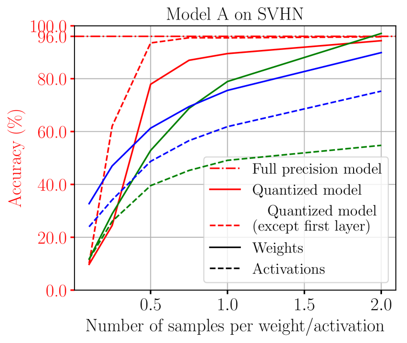
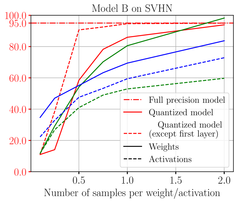
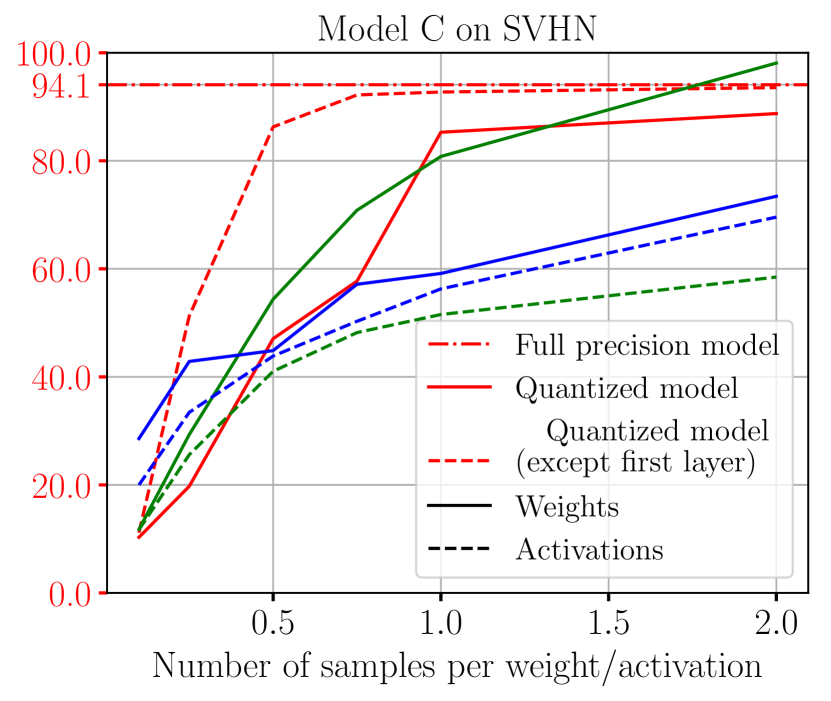
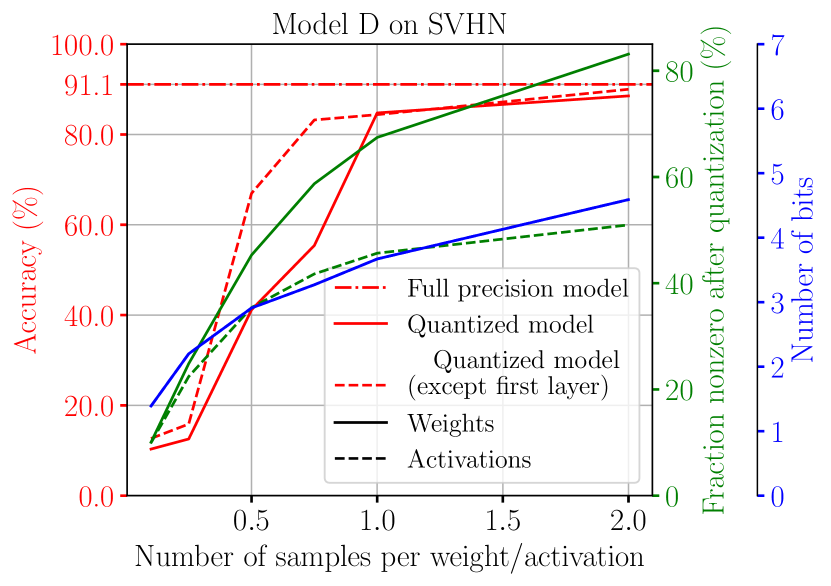
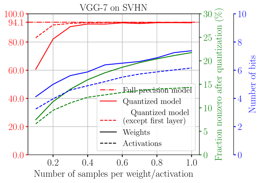
Figure 3: Results of quantizing both weights and activations on SVHN using different sampling amounts. The quantized VGG-7* model reaches close to full-precision accuracy using around 0.5 samples per weight/activation, requiring around 8 bits and using 22% of the weights of the original model, with 22% nonzero activations. Model A, B, C, and D are less redundant models that require more sampling to achieve close to full-precision accuracy.

5.3 ImageNet

For ImageNet, we evaluate MCQ on AlexNet, ResNet-18, and ResNet-50 using the pre-trained models provided by Pytorch’s model zoo [27]). Table 3 shows the results on ImageNet with $K=5.0$ for the different models. The results shown for DoReFa, BWN, TWN [43, 28, 15] are the ones reported in TTQ [44].

Figure 4 shows the accuracy of the quantized model when using different sample sizes, i.e., $K\in\left[0.25,...,5.0\right]$. We observe that more sampling is required to achieve a close to full-precision model accuracy on ImageNet. On this dataset, sorting the CDF before sampling didn’t result in any improvements, so reported results are without sorting. All the quantized models achieve close to full-precision accuracy, though more samples are required than for the previous datasets resulting in a higher required bit-width.

Table 3: Accuracy results on ImageNet when quantizing weights, activations, or both. When quantizing weights only, accuracy drops less than 1% in all tested models. Quantizing only the activations generally leads to a lower accuracy loss compared to quantizing weights. Quantizing both weights and activations leads to an additional accuracy loss of $0.6\%$ in the worst case, i.e. ResNet-50.

Method AlexNet ResNet-18 ResNet-50 Full Precision (32w-32a) 56.52 69.76 76.13 $\Delta$ MCQ (quantized w) -0.99 (8.00w-32a) / -0.681 (8.00w-32a) -0.72 (8.00w-32a)/ -0.631 (8.00w-32a) -0.73 (8.28w-32a)/ -0.201 (8.28w-32a) $\Delta$ MCQ (quantized a) +0.021 (32w-8.36a) -0.581 (32w-7.36a) -0.761 (32w-7.45a) $\Delta$ MCQ (quantized w + a) -1.05 (7.88w-8.46a) / -0.751 (8.00w-7.2a) -1.13 (8.00w-7.35a) /-1.031 (8.00w-7.36a) -1.64 (8.26w-7.43a) / -1.211 (8.28w-7.45a) $\Delta$ FGQ (2w-8a) -7.793 - -4.29 $\Delta$ TTQ (2w-32a) +0.31^,2 -3.01^,2 - $\Delta$ TWNs (2w-32a) -2.71^,2 -4.31^,2 - $\Delta$ BWN (1w-32a) +0.2 -8.51^,2 - $\Delta$ XNOR-Net (1w-1a) -12.4 -18.11^,2 - $\Delta$ DoReFa (1w-32a) -3.31^,2 - - $\Delta$ INQ (5w-32a) -0.15 -0.71 -1.59 $\Delta$ RQ (8w-8a) - +0.43 - $\Delta$ LR-net (2w-32a) - -6.071 -

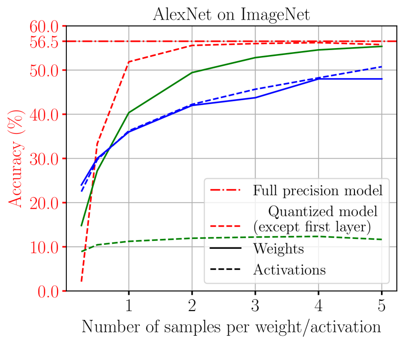
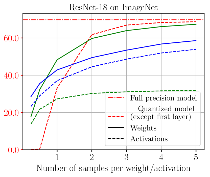
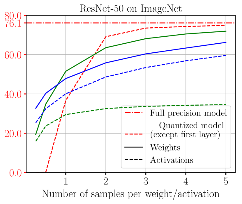
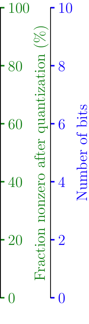
Figure 4: Results of quantizing both weights and activations on ImageNet using different sampling amounts. All quantized models reach close to full-precision accuracy at $K=3$.

5.4 Experiments on additional tasks

To assess the robustness of MCQ, we further evaluate MCQ on several models in natural language and speech processing. We evaluate language modeling on Wikitext-103 using a Transformer-based model [2] and Wikitext-2 using a 2-layer LSTM [41], speech recognition on VCTK using Deepspeech2 [1], and machine translation on WMT-14 English-to-French using a Transformer [26]. Additional details are provided in the Appendix. Table 4 shows the comparison to full-precision models for these various tasks.

Table 4: Evaluation of MCQ on language modeling, speech recognition, and machine translation. All quantized models reach close to full precision performance. Note that, as opposed to the image classification task, we did not study different sampling amounts nor the effect of quantization on specific network layers. A more in-depth analysis could then help to achieve close to full-precision accuracy at a lower bit-width on these models.

Task Dataset Model Metric Full Precision (32w-32a) $\Delta$ MCQ (quantized w) Language Modeling WikiText-103 Transformer Perplexity $\downarrow$ 18.7 +0.21 (8.21w-32a) Language Modeling WikiText-2 LSTM 2x650 Perplexity $\downarrow$ 71.05 +0.51 (7.17w-32a) Speech Recognition VCTK DeepSpeech2 CER $\downarrow$ 7.00 +0.09 (7.26w-32a) Machine Translation WMT14 en-fr Transformer BLEU $\uparrow$ 40.83 -0.23 (7.71w-32a)

6 Discussion and Future Work

The experimental results show the performance of MCQ on multiple models, datasets, and tasks, demonstrated by the minimal loss of accuracy compared to the full-precision counterparts. MCQ either outperforms or is competitive to other methods that require additional training of the quantized network. Moreover, the trade-off between accuracy, sparsity, and bit-width can be easily controlled by adjusting the number of samples. Note that the complexity of the resulting quantized network is proportional to the number of samples in both space and time.

One limitation of MCQ, however, is that it often requires a higher number of bits to represent the quantized values. On the other hand, this sampling-based approach directly translates to a good approximation of the real full-precision values without any additional training. Recently Zhao et al. [41] proposed to outlier channel splitting, which is orthogonal work to MCQ and could be used to reduce the bit-width required for the highest hit counts.

There are several paths that could be worth following for future investigations. In the importance sampling stage, using more sophisticated metrics for importance ranking, e.g. approximation of the Hessian by Taylor expansion could be beneficial  [23]. Automatically selecting optimal sampling levels on each layer could lead to a lower cost since later layers seem to tolerate more sparsity and noise. For efficient hardware implementation, it’s important that the quantized network can be executed using integer operations only. Bias quantization and rescaling, activation rescaling to prevent overflow or underflow, and quantization of errors and gradients for efficient training leave room for future work.

7 Conclusion

In this work, we showed that Monte Carlo sampling is an effective technique to quickly and efficiently convert floating-point, full-precision models to integer, low bit-width models. Computational cost and sparsity can be traded for accuracy by adjusting the number of sampling accordingly.

Our method is linear in both time and space in the number of weights and activations, and is shown to achieve similar results as the full-precision counterparts, for a variety of network architectures, datasets, and tasks. In addition, MCQ is very easy to use for quantizing and sparsifying any pre-trained model. It requires only a few additional lines of code and runs in a matter of seconds depending on the model size, and requires no additional training. The use of sparse, low-bitwidth integer weights and activations in the resulting quantized networks lends itself to efficient hardware implementations.

Appendix A Algorithm

An overview of the proposed method is given in Algorithm 1.

Input: Pre-trained full-precision network

Output: Quantized network with integer weights

for K=0 to L-1 do

       $unsorted_{idxs}\leftarrow argsort(W_{K})$;

       $W_{sorted}\leftarrow sort(W_{K})$;

       $W_{abs}\leftarrow abs(W_{sorted})$;

       // Create PDF

       $W_{PDF}\leftarrow\dfrac{W_{abs}}{\|W_{K}\|_{1}}$;

       // Create CDF

       $W_{CDF}\leftarrow\sum_{i=1}^{|W_{PDF}|}W_{PDF_{i}}$;

       $N\leftarrow ceil(|W_{K}|*K)$;

       $start_{idx}\leftarrow 0$;

       $\xi\leftarrow random(0,1)$ ;

       // Initialize discrete weights with zeros

       $W^{\prime}_{K}\leftarrow[0]\times|W_{K}|$;

       // Start subsampling

       for i=0 to $N-1$ do

             $x_{i}\leftarrow\dfrac{i+\xi}{N}$;

             $hit_{idx}\leftarrow argmax(W_{CDF}[start_{idx}:]\geq x_{i})+start_{idx}$;

             $start_{idx}\leftarrow hit_{idx}$;

            

            $unsorted_{idx}\leftarrow unsorted_{idxs}[hit_{idx}]$

            // Update counter

             if $W_{K}[unsorted_{idx}]>0$ then

                   $W^{\prime}_{K}[unsorted_{idx}]\texttt{++}$;

            else

                   $W^{\prime}_{K}[unsorted_{idx}]\texttt{--}$;

             end if

            

       end for

      

      // Update to integer weights

       $W_{K}\leftarrow W^{\prime}_{K}$;

       // Update layer’s precision

       $B_{W_{K}}\leftarrow 1+floor(\log_{2}(max(abs(W^{\prime}_{K}))))+1$ ;

      

end for

Algorithm 1 Monte Carlo Quantization (MCQ) on network weights. $L$ represents the number of trainable layers, $K$ indicates the percentage of samples to be sampled per weight. The process is performed equivalently for quantizing activations at inference time. Our algorithm is linear in both time and space in the number of weights and activations.

Appendix B Avoiding Exploding Activations

When using integer weights, care has to be taken to avoid overflows in the activations. For that, activations can be scaled using a dynamically computed shifting factor as in [39]. With Monte Carlo sampling, since we know the expected value of the next-layer activations, we can scale accordingly.

$$\mathbf{E}(I_{0,i}) =\frac{N_{samples_{I}}}{N_{I}} \mathbf{E}(W_{0,j}) =\frac{N_{samples_{W_{0}}}}{N_{I}\cdot N_{L_{1}}}$$ (3)

With the activation equation presented in Section 3.1 and $N_{I}$ connections from the input layer to every neuron in the second layer:

$$\begin{split}\mathbf{E}(|a_{l,j}|)=\sum_{i=0}^{N_{I}-1}\mathbf{E}(W_{0,j})\cdot\mathbf{E}(I_{0,i})\end{split}$$ (4)

With $N_{samples_{W_{0}}}=K_{w}\cdot(N_{I}\cdot N_{L_{1}})$ and $N_{samples_{I}}=K_{a}\cdot N_{I}$:

$$\begin{split}\mathbf{E}(|a_{l,j}|)=N_{I}\cdot\frac{K_{w}\cdot(N_{I}\cdot N_{L_{1}})\cdot K_{a}\cdot N_{I}}{N_{I}\cdot N_{L_{1}}\cdot N_{I}}=N_{I}\cdot K_{w}\cdot K_{a}\end{split}$$ (5)

The activations of a neuron need to be scaled by its number of inputs (the receptive field $F_{in}$), multiplied with the number of samples per weight and the number of samples per activation. This is also valid for neurons in convolutional layers, where the receptive field is 3D, e.g. $3\times 3\times 128$.

Moreover, care must be taken to scale biases correctly, by taking both the scaling of weights and activations into account:

$$bias_{scaled}=bias\cdot\frac{N_{samples}}{\|W_{orig}\|_{1}}\cdot\frac{1}{F_{in}}$$ (6)

Appendix C Full-Precision Models Training Details

The architectures and training details of all tested models for CIFAR-10, SVHN, and ImageNet are presented in Sections C.1, C.2, and C.3, respectively. Details of the additional experiments presented in Section 5.4 are shown in Sections C.4, C.5, and C.6.

C.1 CIFAR-10

We trained our full-precision baseline models on the CIFAR-10 dataset [11], consisting of 50000 training samples. We evaluated both our full-precision and quantized models similarly on the rest of the 10000 testing samples. The full-precision VGG-7 ($2\times 128C3-MP2-2\times 256C3-MP2-2\times 512C3-MP2-1024FC-Softmax$) and VGG-14 ($2\times 64C3-MP2-2\times 128C3-MP2-3\times 256C3-MP2-3\times 512C3-MP2-3\times 512C3-MP2-1024FC-Softmax$) models were trained using the code at https://github.com/bearpaw/pytorch-classification. Each was trained for 300 epochs with the Adam optimizer, with a learning rate starting at 0.1 and decreased by factor 10 at epochs 150 and 225, batch size of 128, and weights decay of 0.0005. The ResNet-20 model uses the standard configuration described [9], with 64, 128 and 256 filters in the respective residual blocks. We used more filters to increase the number of available weights in the first block to sample from. This could be similarly performed by sampling more on this specific model to reduce the accuracy loss. The ResNet-20 model is trained using the same hyperparameter settings as the VGG models.

C.2 SVHN

We trained our full-precision baseline models on the Street View House Numbers (SVHN) dataset [25], consising of 73257 training samples. We evaluated both our full-precision and quantized models similarly using the 26032 testing samples provided in this dataset. The full-precision VGG-7* model ($2\times 64C3-MP2-2\times 128C3-MP2-2\times 256C3-MP2-1024FC-Softmax$) was trained for 164 epochs, using the Adam optimizer with learning rate starting at 0.001 and divided by 10 at epochs 80 and 120, weight decay 0.001, and batch size 200. Models A ($48C3-MP2-2\times 64C3-MP2-3\times 128C3-MP2-512C3-Softmax$), B, C, and D were trained using the code at https://github.com/aaron-xichen/pytorch-playground and the same hyperparameter settings as VGG-7* but trained for 200 epochs.

C.3 ImageNet

We evaluated both our full-precision and quantized models similarly on the validation set of the ILSVRC12 classification dataset [5], consisting of 50K validation images. The full-precision pre-trained models are taken from Pytorch’s model zoo https://pytorch.org/docs/stable/torchvision/models.html [27].

C.4 VCTK

CSTR’s VCTK Corpus (Centre for Speech Technology Voice Cloning Toolkit) includes speech data uttered by 109 native speakers of English with various accents, where each speaker reads out about 400 sentences, most of which were selected from a newspaper. The evaluated model uses 2 convolutional layers and 5 GRU layers of 768 hidden units, using code from https://github.com/SeanNaren/deepspeech.pytorch [35].

C.5 Wikitext

The WikiText language modeling dataset is a collection of over 100 million tokens extracted from the set of verified Good and Featured articles on Wikipedia. Compared to the preprocessed version of Penn Treebank (PTB), WikiText-2 is over 2 times larger and WikiText-103 is over 110 times larger. The WikiText dataset also features a far larger vocabulary and retains the original case, punctuation and numbers - all of which are removed in PTB. As it is composed of full articles, the dataset is well suited for models that can take advantage of long term dependencies. The WikiText-2 model was a 2-layer LSTM with 650 hidden neurons, and an embedding size of 400. It was trained using the setup and code at https://github.com/salesforce/awd-lstm-lm [21]. The WikiText-102 model was a pretrained model available at https://github.com/pytorch/fairseq/tree/master/examples/language_model, along with evaluation code [2].

C.6 NMT

The dataset is WMT’14 English-French, cmobining data from several other corpuses, amongst others the Europarl corpus, the News Commentary corpus, and the Common Crawl corpus [18]. The model was a pretrained model available at https://github.com/pytorch/fairseq/tree/master/examples/scaling_nmt, along with evaluation code [26].

Appendix D Quantizing Weights Only

Figures 5, 6, and 7 show the effects of varying the amounts of sampling when quantizing only the weights.

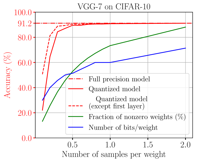
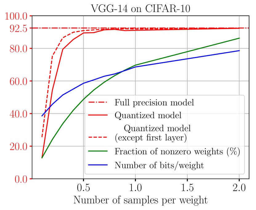
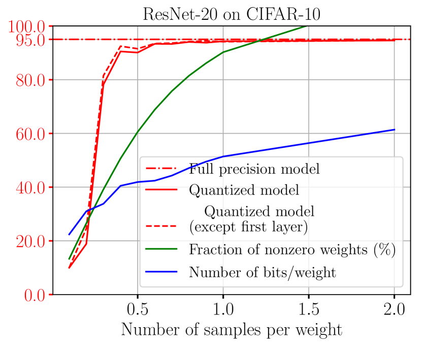
Figure 5: Quantized weights on CIFAR-10

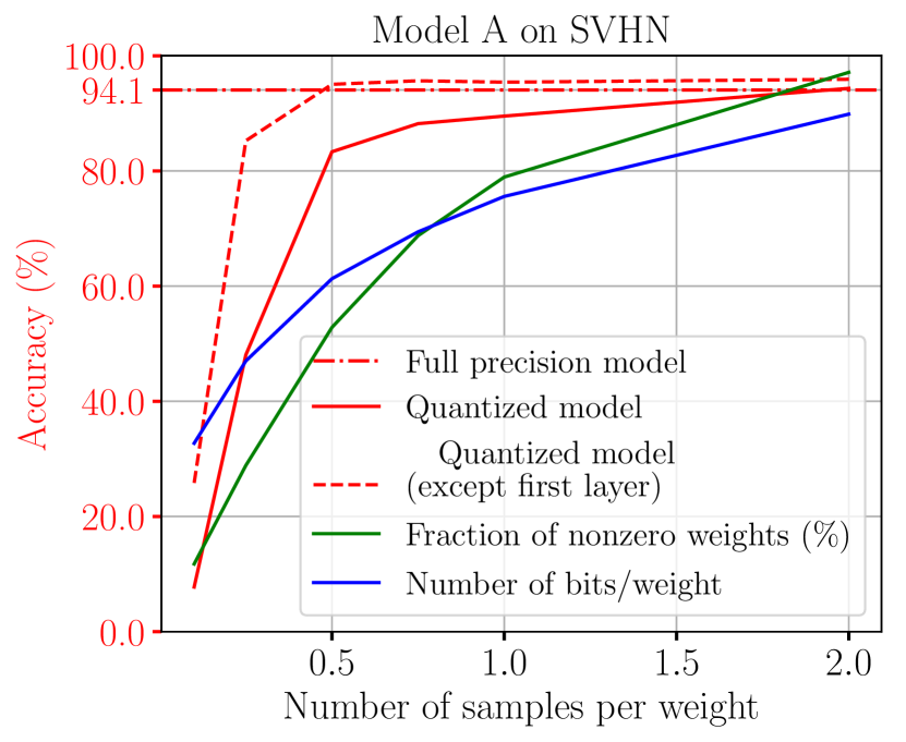
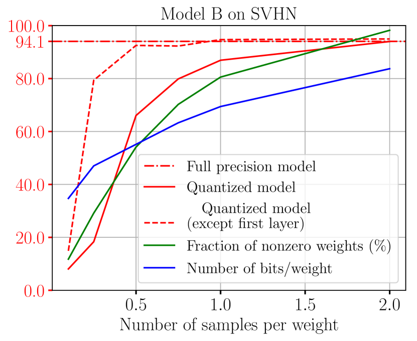
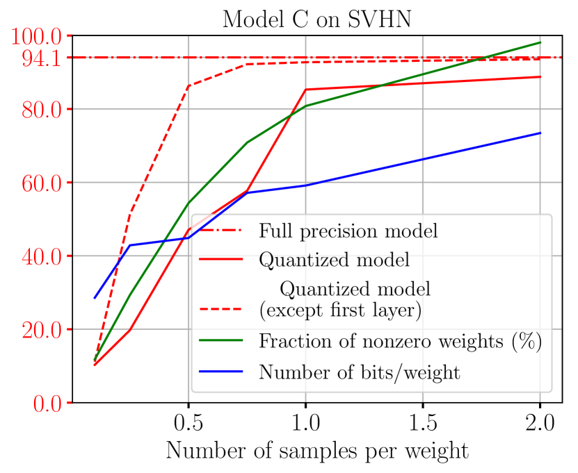
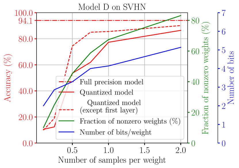
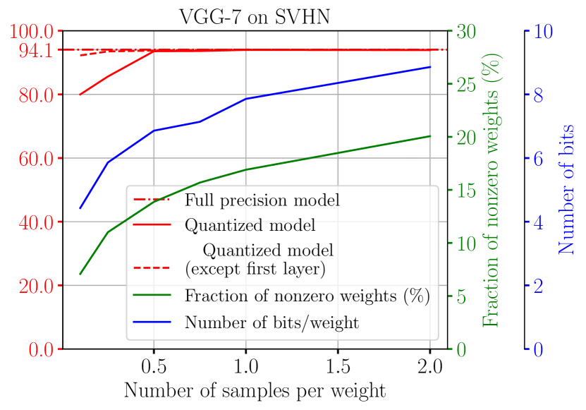
Figure 6: Quantized weights on SVHN

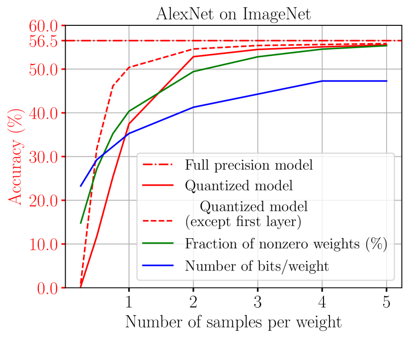
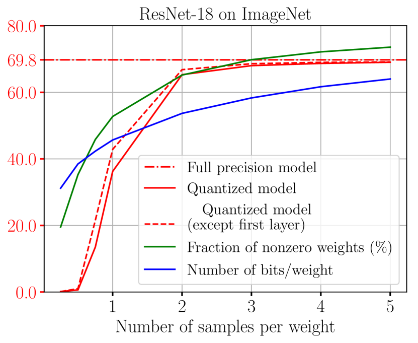
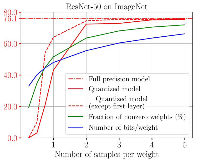
Figure 7: Quantized weights on ImageNet

Appendix E Quantizing Activations Only

Figures 8, 9, and 10 show the effects of varying the amounts of sampling when quantizing only the activations. We observe less sampling is required to achieve full-precision accuracy when quantizing only the activations when compared to quantizing the weights only.

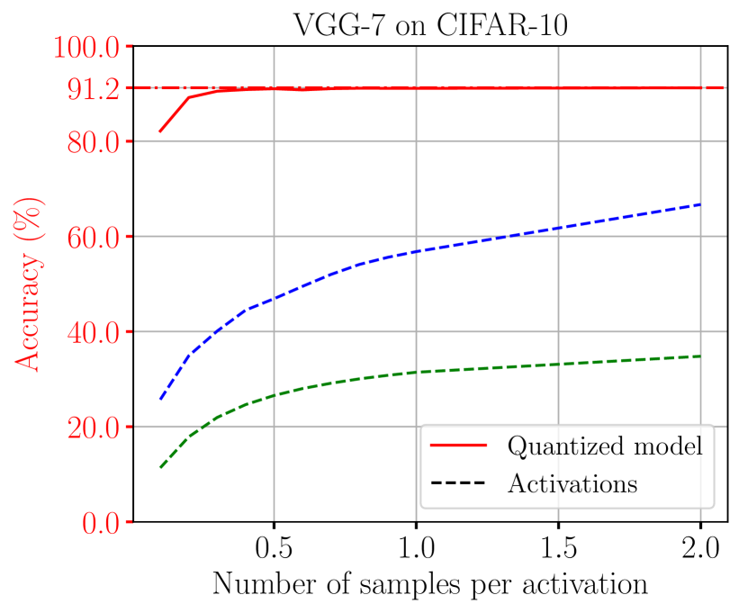
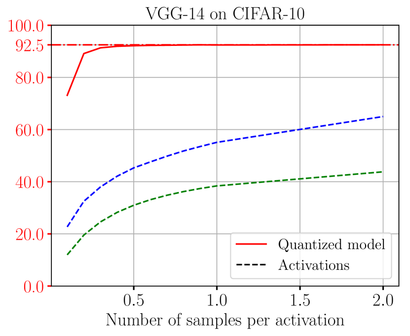
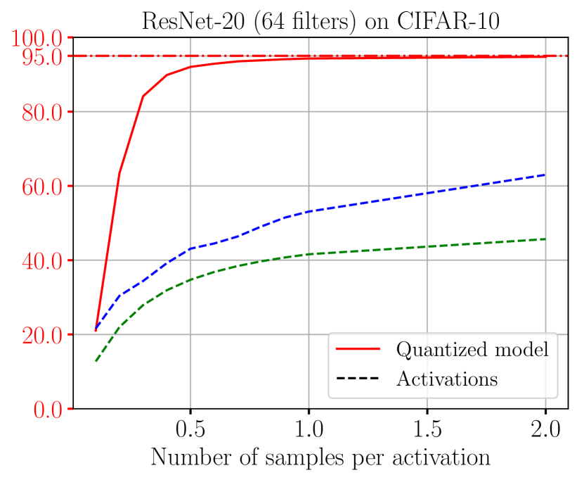
Figure 8: Quantized activations on CIFAR-10

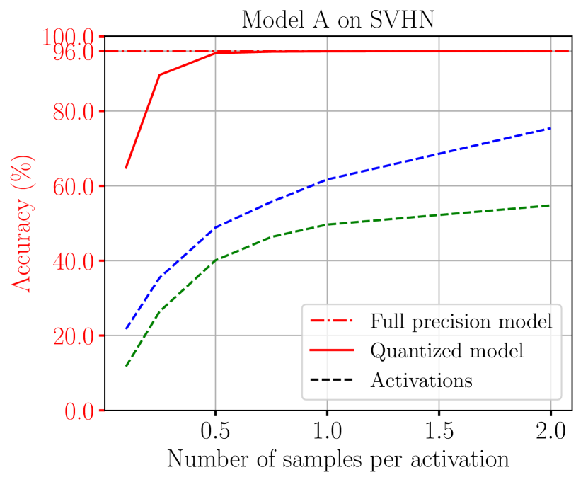
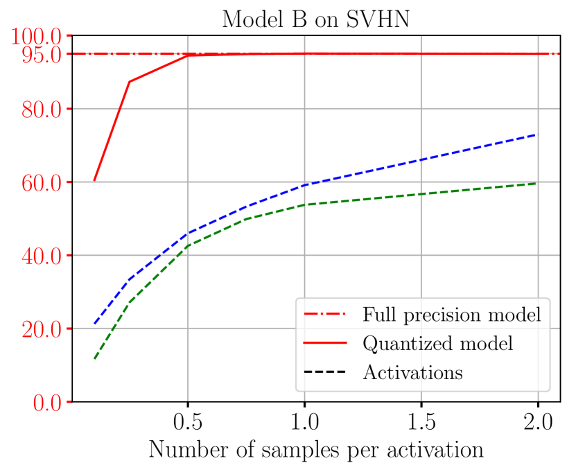
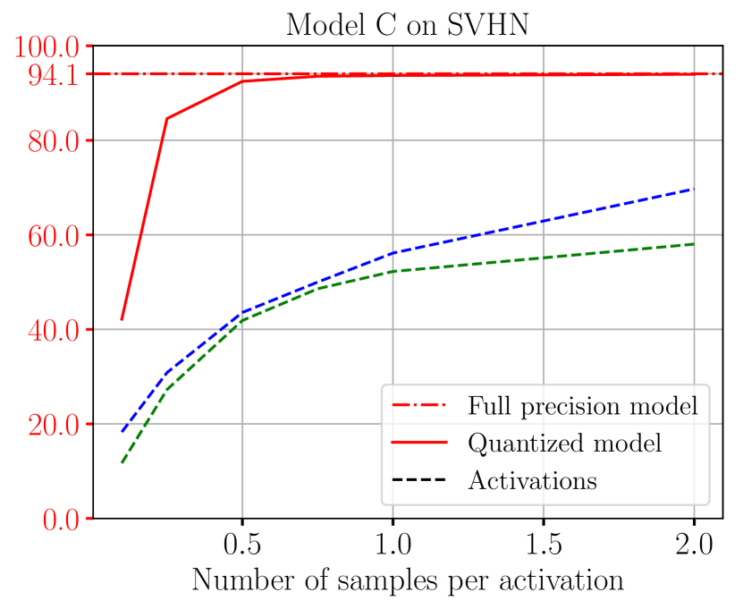
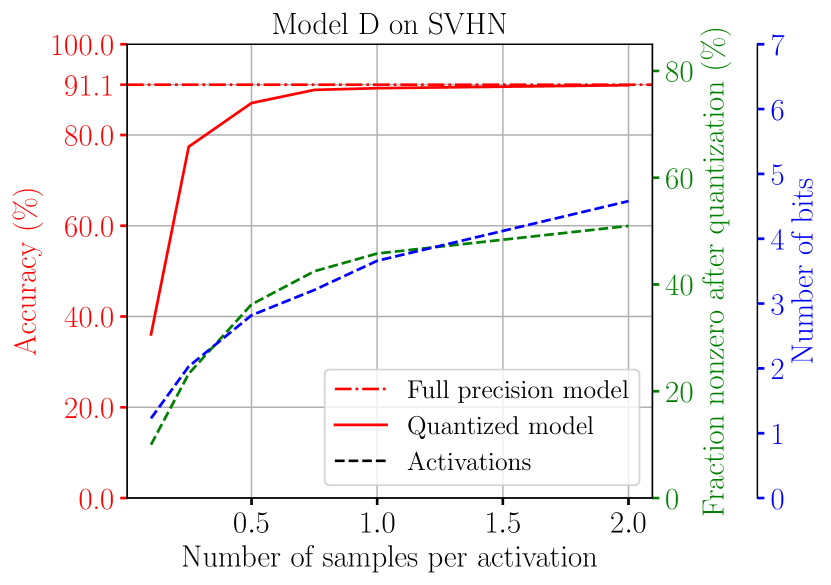
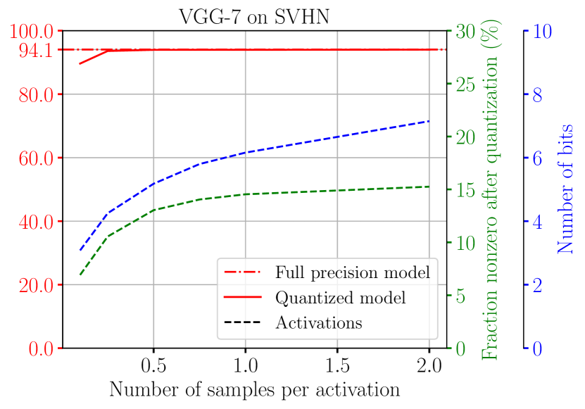
Figure 9: Quantized activations on SVHN

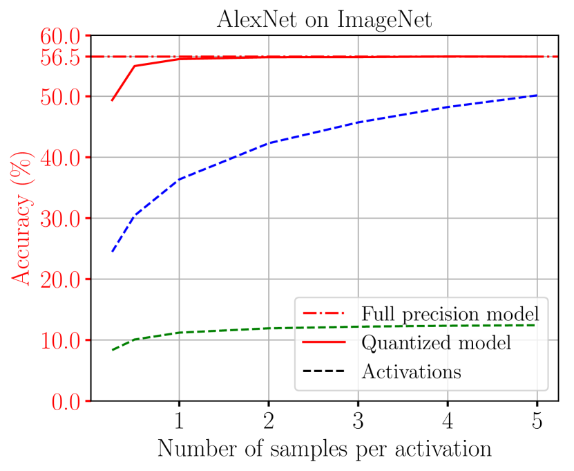
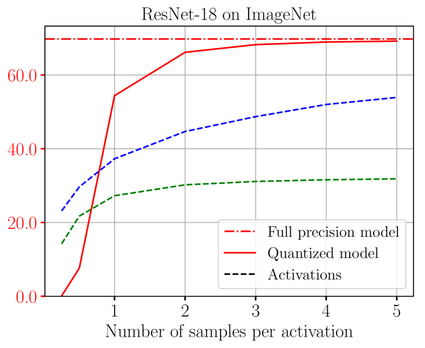
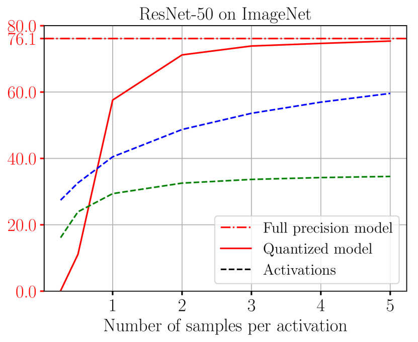
Figure 10: Quantized activations on ImageNet

Appendix F Effects of Different Sampling Seeds

In a small experiment on CIFAR-10, we observe that using different sampling seeds can result in up to a $\approx 0.5\%$ absolute variation in accuracy of the different quantized networks (Figure 11). Grid searching over several sampling seeds may then be beneficial to achieve a better quantized model in the end, depending on the use-case.

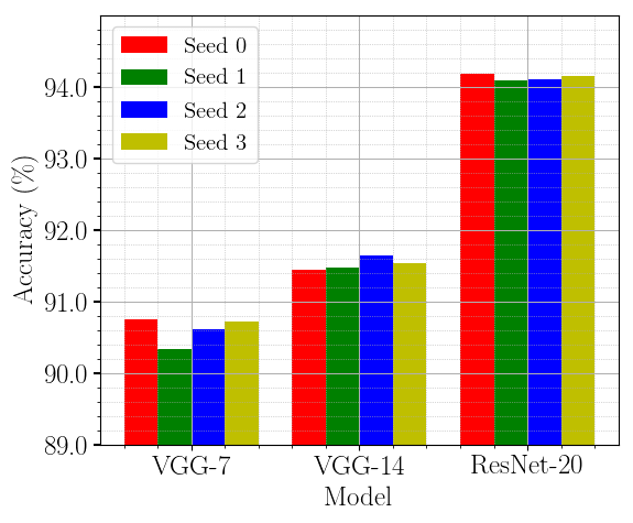
(a) Quantized weights

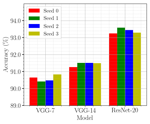
(b) Quantized weights and activations

Figure 11: Different sampling seeds on CIFAR-10 with $K=1.0$.

References

- Amodei et al. [2015] Dario Amodei, Rishita Anubhai, Eric Battenberg, Carl Case, Jared Casper, Bryan Catanzaro, Jingdong Chen, Mike Chrzanowski, Adam Coates, Greg Diamos, Erich Elsen, Jesse H. Engel, Linxi Fan, Christopher Fougner, Tony Han, Awni Y. Hannun, Billy Jun, Patrick LeGresley, Libby Lin, Sharan Narang, Andrew Y. Ng, Sherjil Ozair, Ryan Prenger, Jonathan Raiman, Sanjeev Satheesh, David Seetapun, Shubho Sengupta, Yi Wang, Zhiqian Wang, Chong Wang, Bo Xiao, Dani Yogatama, Jun Zhan, and Zhenyao Zhu. Deep speech 2: End-to-end speech recognition in english and mandarin. CoRR, abs/1512.02595, 2015. URL http://arxiv.org/abs/1512.02595.
- Baevski and Auli [2018] Alexei Baevski and Michael Auli. Adaptive input representations for neural language modeling. CoRR, abs/1809.10853, 2018. URL http://arxiv.org/abs/1809.10853.
- Courbariaux et al. [2014] Matthieu Courbariaux, Yoshua Bengio, and Jean-Pierre David. Training deep neural networks with low precision multiplications. arXiv preprint arXiv:1412.7024, 2014.
- Courbariaux et al. [2015] Matthieu Courbariaux, Yoshua Bengio, and Jean-Pierre David. Binaryconnect: Training deep neural networks with binary weights during propagations. In Advances in neural information processing systems, pages 3123–3131, 2015.
- Deng et al. [2009] J. Deng, W. Dong, R. Socher, L.-J. Li, K. Li, and L. Fei-Fei. ImageNet: A Large-Scale Hierarchical Image Database. In CVPR09, 2009.
- Goodfellow et al. [2014] Ian Goodfellow, Jean Pouget-Abadie, Mehdi Mirza, Bing Xu, David Warde-Farley, Sherjil Ozair, Aaron Courville, and Yoshua Bengio. Generative adversarial nets. In Advances in neural information processing systems, pages 2672–2680, 2014.
- Gupta et al. [2015] Suyog Gupta, Ankur Agrawal, Kailash Gopalakrishnan, and Pritish Narayanan. Deep learning with limited numerical precision. In Francis Bach and David Blei, editors, Proceedings of the 32nd International Conference on Machine Learning, volume 37 of Proceedings of Machine Learning Research, pages 1737–1746, Lille, France, 07–09 Jul 2015. PMLR.
- Han et al. [2015] Song Han, Huizi Mao, and William J Dally. Deep compression: Compressing deep neural networks with pruning, trained quantization and Huffman coding. arXiv preprint arXiv:1510.00149, 2015.
- He et al. [2016] Kaiming He, Xiangyu Zhang, Shaoqing Ren, and Jian Sun. Deep residual learning for image recognition. In The IEEE Conference on Computer Vision and Pattern Recognition (CVPR), June 2016.
- Hubara et al. [2016] Itay Hubara, Matthieu Courbariaux, Daniel Soudry, Ran El-Yaniv, and Yoshua Bengio. Binarized neural networks. In Advances in neural information processing systems, pages 4107–4115, 2016.
- Krizhevsky and Hinton [2009] Alex Krizhevsky and Geoffrey Hinton. Learning multiple layers of features from tiny images. Technical report, Citeseer, 2009.
- LeCun et al. [1990] Yann LeCun, John S Denker, and Sara A Solla. Optimal brain damage. In Advances in neural information processing systems, pages 598–605, 1990.
- L’Ecuyer et al. [2008] Pierre L’Ecuyer, Christian Lécot, and Bruno Tuffin. A randomized quasi-Monte Carlo simulation method for Markov chains. Operations Research, 56(4):958–975, 2008.
- L’Ecuyer et al. [2018] Pierre L’Ecuyer, David Munger, Christian Lécot, and Bruno Tuffin. Sorting methods and convergence rates for Array-RQMC: some empirical comparisons. Mathematics and Computers in Simulation, 143:191–201, 2018.
- Li et al. [2016] Fengfu Li, Bo Zhang, and Bin Liu. Ternary weight networks. arXiv preprint arXiv:1605.04711, 2016.
- Lin et al. [2015] Zhouhan Lin, Matthieu Courbariaux, Roland Memisevic, and Yoshua Bengio. Neural networks with few multiplications. arXiv preprint arXiv:1510.03009, 2015.
- Louizos et al. [2018] Christos Louizos, Matthias Reisser, Tijmen Blankevoort, Efstratios Gavves, and Max Welling. Relaxed quantization for discretized neural networks. arXiv preprint arXiv:1810.01875, 2018.
- Machacek and Bojar [2014] Matous Machacek and Ondrej Bojar. Results of the wmt14 metrics shared task. In Proceedings of the Ninth Workshop on Statistical Machine Translation, pages 293–301, 2014.
- Mellempudi et al. [2017] Naveen Mellempudi, Abhisek Kundu, Dheevatsa Mudigere, Dipankar Das, Bharat Kaul, and Pradeep Dubey. Ternary neural networks with fine-grained quantization. arXiv preprint arXiv:1705.01462, 2017.
- Merity et al. [2017a] Stephen Merity, Nitish Shirish Keskar, and Richard Socher. Regularizing and optimizing LSTM language models. CoRR, abs/1708.02182, 2017a. URL http://arxiv.org/abs/1708.02182.
- Merity et al. [2017b] Stephen Merity, Nitish Shirish Keskar, and Richard Socher. Regularizing and optimizing LSTM language models. CoRR, abs/1708.02182, 2017b. URL http://arxiv.org/abs/1708.02182.
- Mocanu et al. [2018] Decebal Constantin Mocanu, Elena Mocanu, Peter Stone, Phuong H Nguyen, Madeleine Gibescu, and Antonio Liotta. Scalable training of artificial neural networks with adaptive sparse connectivity inspired by network science. Nature communications, 9(1):2383, 2018.
- Molchanov et al. [2016] Pavlo Molchanov, Stephen Tyree, Tero Karras, Timo Aila, and Jan Kautz. Pruning convolutional neural networks for resource efficient inference. arXiv preprint arXiv:1611.06440, 2016.
- Nair and Hinton [2010] Vinod Nair and Geoffrey E Hinton. Rectified linear units improve restricted boltzmann machines. In Proceedings of the 27th international conference on machine learning (ICML-10), pages 807–814, 2010.
- Netzer et al. [2011] Yuval Netzer, Tao Wang, Adam Coates, Alessandro Bissacco, Bo Wu, and Andrew Y Ng. Reading digits in natural images with unsupervised feature learning. Neural Information Processing Systems, 2011.
- Ott et al. [2018] Myle Ott, Sergey Edunov, David Grangier, and Michael Auli. Scaling neural machine translation. CoRR, abs/1806.00187, 2018. URL http://arxiv.org/abs/1806.00187.
- Paszke et al. [2017] Adam Paszke, Sam Gross, Soumith Chintala, Gregory Chanan, Edward Yang, Zachary DeVito, Zeming Lin, Alban Desmaison, Luca Antiga, and Adam Lerer. Automatic differentiation in pytorch. In NIPS-W, 2017.
- Rastegari et al. [2016] Mohammad Rastegari, Vicente Ordonez, Joseph Redmon, and Ali Farhadi. Xnor-net: Imagenet classification using binary convolutional neural networks. In European Conference on Computer Vision, pages 525–542. Springer, 2016.
- Reagen et al. [2017] Brandon Reagen, Udit Gupta, Robert Adolf, Michael M Mitzenmacher, Alexander M Rush, Gu-Yeon Wei, and David Brooks. Weightless: Lossy weight encoding for deep neural network compression. arXiv preprint arXiv:1711.04686, 2017.
- Robbins and Monro [1951] Herbert Robbins and Sutton Monro. A stochastic approximation method. The annals of mathematical statistics, pages 400–407, 1951.
- Salimans and Kingma [2016] Tim Salimans and Diederik P. Kingma. Weight normalization: A simple reparameterization to accelerate training of deep neural networks. CoRR, abs/1602.07868, 2016. URL http://arxiv.org/abs/1602.07868.
- Shayer et al. [2017] Oran Shayer, Dan Levi, and Ethan Fetaya. Learning discrete weights using the local reparameterization trick. arXiv preprint arXiv:1710.07739, 2017.
- Srivastava et al. [2014] Nitish Srivastava, Geoffrey Hinton, Alex Krizhevsky, Ilya Sutskever, and Ruslan Salakhutdinov. Dropout: a simple way to prevent neural networks from overfitting. The Journal of Machine Learning Research, 15(1):1929–1958, 2014.
- Strubell et al. [2019] Emma Strubell, Ananya Ganesh, and Andrew McCallum. Energy and policy considerations for deep learning in NLP. CoRR, abs/1906.02243, 2019. URL http://arxiv.org/abs/1906.02243.
- Veaux et al. [2017] Christophe Veaux, Junichi Yamagishi, Kirsten MacDonald, et al. Cstr vctk corpus: English multi-speaker corpus for cstr voice cloning toolkit. University of Edinburgh. The Centre for Speech Technology Research (CSTR), 2017.
- Venkatesh et al. [2017] Ganesh Venkatesh, Eriko Nurvitadhi, and Debbie Marr. Accelerating deep convolutional networks using low-precision and sparsity. In 2017 IEEE International Conference on Acoustics, Speech and Signal Processing (ICASSP), pages 2861–2865. IEEE, 2017.
- Wan et al. [2013] Li Wan, Matthew Zeiler, Sixin Zhang, Yann Le Cun, and Rob Fergus. Regularization of neural networks using dropconnect. In International conference on machine learning, pages 1058–1066, 2013.
- Wang et al. [2019] Kuan Wang, Zhijian Liu, Yujun Lin, Ji Lin, and Song Han. Haq: Hardware-aware automated quantization with mixed precision. In Proceedings of the IEEE Conference on Computer Vision and Pattern Recognition, pages 8612–8620, 2019.
- Wu et al. [2018] Shuang Wu, Guoqi Li, Feng Chen, and Luping Shi. Training and inference with integers in deep neural networks. CoRR, abs/1802.04680, 2018. URL http://arxiv.org/abs/1802.04680.
- Zhang et al. [2018] Dongqing Zhang, Jiaolong Yang, Dongqiangzi Ye, and Gang Hua. Lq-nets: Learned quantization for highly accurate and compact deep neural networks. In Proceedings of the European Conference on Computer Vision (ECCV), pages 365–382, 2018.
- Zhao et al. [2019] Ritchie Zhao, Yuwei Hu, Jordan Dotzel, Christopher De Sa, and Zhiru Zhang. Improving neural network quantization without retraining using outlier channel splitting. CoRR, abs/1901.09504, 2019. URL http://arxiv.org/abs/1901.09504.
- Zhou et al. [2017] Aojun Zhou, Anbang Yao, Yiwen Guo, Lin Xu, and Yurong Chen. Incremental network quantization: Towards lossless cnns with low-precision weights. arXiv preprint arXiv:1702.03044, 2017.
- Zhou et al. [2016] Shuchang Zhou, Yuxin Wu, Zekun Ni, Xinyu Zhou, He Wen, and Yuheng Zou. Dorefa-net: Training low bitwidth convolutional neural networks with low bitwidth gradients. arXiv preprint arXiv:1606.06160, 2016.
- Zhu et al. [2016] Chenzhuo Zhu, Song Han, Huizi Mao, and William J Dally. Trained ternary quantization. arXiv preprint arXiv:1612.01064, 2016.