Control limit on quantum state preparation under decoherence

Abstract

Quantum information technologies require careful control for generating and preserving a desired target quantum state. The biggest practical obstacle is, of course, decoherence. Therefore, the reachability analysis, which in our scenario aims to estimate the distance between the controlled state under decoherence and the target state, is of great importance to evaluate the realistic performance of those technologies. This paper presents a lower bound of the fidelity-based distance for a general open Markovian quantum system driven by the decoherence process and several types of control including feedback. The lower bound is straightforward to calculate and can be used as a guide for choosing the target state, as demonstrated in some examples. Moreover, the lower bound is applied to derive a theoretical limit in some quantum metrology problems based on a large-size atomic ensemble under control and decoherence.

I Introduction

There is no doubt that a carefully designed control plays a key role in quantum information science. The open-loop (i.e., non-feedback) control theory Rabitz 1993 ; Viola 1999 ; Khaneja 2003 ; D'Alessandro Book ; Jacobs 2007 ; Jacobs 2009 ; Montangero PRL 2011 ; Laflamme 2016 offers several powerful means, for example, for implementing an efficient quantum gate operation. The measurement-based feedback (MBF) Stockton 2004 ; Handel 2005 ; Geremia 2006 ; Yanagisawa 2006 ; Yamamoto 2007 ; Molmer 2007 ; Mirrahimi 2007 ; Bouten 2009 and reservoir engineering including coherent feedback Poyatos 1996 ; Schirmer 2010 ; Yamamoto 2014 ; Vitali2014 ; Clerk2016 ; Combes 2017 ; Ferraro 2018 are also well-established methodologies that can be used for generating and protecting a desired quantum state. Remarkably, many notable experiments realizing those control techniques have been demonstrated Haroche 2011 ; Siddiqi 2012 ; Lehnert 2013 ; Siddiqi 2016 ; Thompson 2016 ; Devoret 2016 , which at the same time show that the actual control performance in the presence of decoherence is sometimes far away from the ideal one. Therefore the reachability analysis is essential to evaluate the practical effectiveness of those control methods; that is, it is important to quantify how close the controlled quantum state can be steered to or preserved at around a target state under decoherence. Note that the reachability characteristic determines a lower bound of the time required for performing a desired state transformation via control Lloyd 2014 .

The reachability analysis found in the literature is usually based on simulations, which numerically investigate how much the ideal state control is disturbed by decoherence; for example, generation of a nano-resonator superposition state via open-loop control Jacobs 2007 ; Jacobs 2009 , an optical Fock state via MBF Geremia 2006 ; Molmer 2007 , and an opto-mechanical cat state via reservoir engineering Vitali2014 ; Ferraro 2018 . The optimal control method is also often used, which numerically designs a time-dependent control input for steering the state closest to the target under decoherence Khaneja 2003 ; Koch 2016 . However, these computational approaches do not give us deep insight into basic questions for quantum engineering, e.g., what state should be targeted, what the limit of realistic state preparation is, and what the desired structure of open quantum systems under given decoherence is. A few exceptions are found for specific types of open-loop control Khaneja pnas 2003 and MBF Guo 2010 ; Guo 2013 , but there has been no unified approach. Also the controllability property, which is a stronger notion than the reachability, can be analytically investigated using the Lie algebra Altafini 2003 ; Khaneja 2009 ; Kurniawan 2009 ; Kurniawan 2012 ; Dirr 2012 ; Yuan 2013 ; but it does not quantify the distance to the target and thus does not answer the above questions.

The main contribution of this paper is to present a limit for reachability, applicable for a general open Markovian quantum system driven by the decoherence process and several types of control including the open-loop and MBF controls and reservoir engineering; more precisely, we give a lower bound of the fidelity-based distance between a given target state and the controlled state under decoherence. This lower bound is straightforward to calculate, without solving any equation. Also thanks to its generic form, the lower bound gives a characterization of target states that are largely affected by the decoherence, and thereby provides us a useful guide for choosing the target, as demonstrated in some examples. Moreover, as “a deep insight into quantum engineering”, the lower bound is used to derive a theoretical limit in quantum metrology; for a typical large-size atomic ensemble under control and decoherence, the fidelity to the target (the Greenberger-Horne-Zeilinger (GHZ) state or a highly entangled Dicke state) must be less than 0.875, regardless of the control strategy.

II The control limit

II.1 Controlled quantum dynamics

We begin with a simplified setting of open-loop control and reservoir engineering; the quantum state $\bar{\rho}_{t}$ obeys the Markovian master equation

$$\frac{d\bar{\rho}_{t}}{dt}=-i[u_{t}H,\bar{\rho}_{t}]+\mathcal{D}[L]\bar{\rho}_{t}+\mathcal{D}[M]\bar{\rho}_{t},$$ (1)

where $H$ is a system Hamiltonian. $L$ and $M$ are Lindblad operators, and hence $\mathcal{D}[A]\bar{\rho}=A\bar{\rho}A^{\dagger}-A^{\dagger}A\bar{\rho}/2-\bar{\rho}A^{\dagger}A/2$. Here $L$ represents the uncontrollable “L”indblad operator corresponding to the decoherence, while $M$ can be engineered; in particular in the MBF setting $M$ represents the probe for “M”easurement. The standard open-loop control problem is to design a time-dependent sequence $u_{t}$ that steers $\bar{\rho}_{t}$ toward a target state, under $M=0$. Also the standard reservoir engineering approach aims to design $M$, with constant $u_{t}$, so that $\bar{\rho}_{t}$ autonomously converges to a target.

The MBF control setting can also be included in the theory. In this case the quantum state $\rho_{t}$ conditioned on the measurement record $y_{t}$ obeys the following stochastic master equation (SME) Wiseman Book ; Jacobs Book ; NY Book :

$$d\rho_{t}=-i[u_{t}H,\rho_{t}]dt+\mathcal{D}[L]\rho_{t}dt+\mathcal{D}[M]\rho_{t}dt+\mathcal{H}[M]\rho_{t}dW_{t},$$ (2)

where $dW_{t}=dy_{t}-{\rm Tr}[(M+M^{\dagger})\rho_{t}]dt$ is the Wiener increment representing the innovation process based on $y_{t}$, and $\mathcal{H}[A]\rho=A\rho+\rho A^{\dagger}-{\rm Tr}[(A+A^{\dagger})\rho]\rho$. The goal of MBF is to design the control signal $u_{t}$ as a function of $\rho_{t}$, to achieve a certain goal. In particular, if $L=0$ and $M=M^{\dagger}$, there are several types of MBF control that selectively steer the state to an arbitrary eigenstate of $M$. In this paper, we focus on the unconditional state $\bar{\rho}_{t}={\mathbb{E}}(\rho_{t})$, which is the ensemble average of $\rho_{t}$ over all the measurement results. Then due to ${\mathbb{E}}(W_{t})=0$, Eq. (2) leads to the following master equation:

$$\frac{d\bar{\rho}_{t}}{dt}=-i[H,{\mathbb{E}}(u_{t}\rho_{t})]+\mathcal{D}[L]\bar{\rho}_{t}+\mathcal{D}[M]\bar{\rho}_{t}.$$ (3)

Note that now $u_{t}$ is a function of $\rho_{t}$, and thus Eq. (3) is not a linear equation with respect to $\bar{\rho}_{t}$. In the open-loop control or reservoir engineering setting, meaning that $u_{t}$ is independent of $\rho_{t}$, then Eq. (3) is reduced to the linear equation (1) due to ${\mathbb{E}}(u_{t}\rho_{t})=u_{t}\bar{\rho}_{t}$.

II.2 Main result

The control goal is to minimize the following cost function:

$$J_{t}=1-\langle{\psi}|\bar{\rho}_{t}|{\psi}\rangle,$$ (4)

where $|{\psi}\rangle$ is the target pure state and $\bar{\rho}_{t}$ is the controlled state obeying Eq. (1) or (3); hence, $J_{t}$ represents the fidelity-based distance of $\bar{\rho}_{t}$ from the target. Under the presence of decoherence term ${\mathcal{D}}[L]$, in general it is impossible to deterministically achieve $J_{t}=0$ at some time $t$. The main result of this paper is to provide a lower bound of the cost in an explicit form as follows. The proof is given in Appendix A.

Theorem 1: The cost (4) has the following lower bound at the steady state:

$$J_{\infty}\geq J_{\ast}(|{\psi}\rangle)=\left(\frac{{\mathcal{E}}}{{\mathcal{A}}+{\mathcal{U}}}\right)^{2},$$ (5)

where ($\||{\psi}\rangle\|^{2}=\langle{\psi}|{\psi}\rangle$ is the Euclidean norm)

$${\mathcal{A}} =\sqrt{2}\bigl{(}\|L^{\dagger}|{\psi}\rangle\|^{2}+\|L^{\dagger}L|{\psi}\rangle\|$$

$$\hskip 28.45274pt+\|M^{\dagger}|{\psi}\rangle\|^{2}+\|M^{\dagger}M|{\psi}\rangle\|\bigr{)},$$

$${\mathcal{U}} =2\bar{u}\sqrt{\langle{\psi}|H^{2}|{\psi}\rangle-\langle{\psi}|H|{\psi}\rangle^{2}},~{}~{}\bar{u}=\max\{|u_{t}|\},$$

$${\mathcal{E}} =\|L|{\psi}\rangle\|^{2}-|\langle{\psi}|L|{\psi}\rangle|^{2}+\|M|{\psi}\rangle\|^{2}-|\langle{\psi}|M|{\psi}\rangle|^{2}.$$

Moreover, if $J_{t_{0}}\geq J_{*}$ for an initial state $\bar{\rho}_{t_{0}}$, then $J_{t}\geq J_{*}$ holds for all $t\in[t_{0},\infty)$.

That is, $J_{*}$ gives a limit on how close the controlled quantum state can be steered to or preserved at around a target state under decoherence. Below we list some notable general features of $J_{*}$.

(i) The theorem is applicable to a general Markovian open quantum systems driven by several types of control including the MBF and reservoir engineering.

(ii) The result can be extended to the case where the system is subjected to multiple environment channels, measurement probes, and control Hamiltonians, as long as the dynamical equation can be validly described as an extension of Eq. (1) or (2); see Appendix B.

(iii) $J_{*}$ is directly computable, once the system operators and the target state $|{\psi}\rangle$ are specified; it is not necessary to solve any equation.

(iv) $J_{*}$ is a monotonically decreasing function of the control magnitude $\bar{u}$.

(v) If $|{\psi}\rangle$ moves away from the eigenstates of $L$ and $M$, then $J_{*}$ becomes bigger. Conversely, $J_{*}=0$ if and only if $|{\psi}\rangle$ is identical to a common eigenvector of $L$ and $M$.

Importantly, $J_{*}$ can be used to characterize a target state that is possibly easy to approach by some control, under a given decoherence. That is, a state $|{\psi}\rangle$ with relatively small value of $J_{*}$ might be a good candidate as the target, although in general $J_{*}$ is not achievable. Conversely, we can safely say that the state $|{\psi}\rangle$ with a relatively large value of $J_{*}$ should not be assigned as the target. In what follows we study some typical control problems, with special attention to this point.

III Examples

III.1 Qubit

The first example is a qubit such as a two-level atom, consisting of $|{e}\rangle=[1,0]^{\top}$ and $|{g}\rangle=[0,1]^{\top}$. Let the target be a pure qubit state

$$|{\psi}\rangle=[\cos{\theta},~{}e^{i\varphi}\sin{\theta}]^{\top},~{}(0\leq\theta<\pi/2,\ 0\leq\varphi<2\pi).$$ (6)

Here we consider the following operators:

$$H=\sigma_{y},~{}M=\sqrt{\kappa}\sigma_{z},~{}L=\sqrt{\gamma}\sigma_{-},$$

where $\sigma_{y}=i(|{g}\rangle\langle{e}|-|{e}\rangle\langle{g}|)$, $\sigma_{z}=|{e}\rangle\langle{e}|-|{g}\rangle\langle{g}|$, and $\sigma_{-}=|{g}\rangle\langle{e}|$. This is a typical MBF control setup Handel 2005 ; Siddiqi 2012 ; Lehnert 2013 ; Siddiqi 2016 ; $M$ represents the engineered dispersive coupling between the qubit and the probe, which enables us to continuously monitor the qubit state by measuring the probe output and thereby perform a MBF control via the Hamiltonian $u_{t}H$. Ideally (i.e., if $\gamma=0$), this MBF realizes deterministic and selective steering of the qubit state to $|{e}\rangle$ or $|{g}\rangle$. However in practice this perfect control is not allowed due to decoherence $L=\sqrt{\gamma}\sigma_{-}$, i.e., energy decay from $|{e}\rangle$ to $|{g}\rangle$ for a two-level atom. In this setup, the lower bound $J_{*}$ is calculated as

$$J_{\ast}=\frac{1}{2}\left[\frac{\kappa\sin^{2}2\theta+\gamma\cos^{4}\theta}{2\kappa+\gamma(\sin^{2}\theta+\cos\theta)+\bar{u}\sqrt{2-2\sin^{2}2\theta\sin^{2}\varphi}}\right]^{2}.$$

A detailed derivation of this expression (and that of $J_{*}$ in the other examples) is provided in Appendix D.

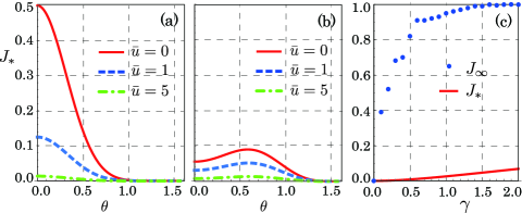
Figure 1: The lower bound $J_{*}$ as a function of $\theta$ for (a) $\kappa=0$ and (b) $\kappa=1$, in units of $\gamma=1$. (c) Plot of $J_{*}$ and $J_{\infty}$ with $u_{t}$ a special type of MBF control input, for the case $|{\psi}\rangle=|{e}\rangle$ and $(\kappa,\bar{u})=(1,1)$.

First, we set $\kappa=0$; this is the case where the system obeys the master equation $d\bar{\rho}_{t}/dt=-i[u_{t}\sigma_{y},\bar{\rho}_{t}]+{\mathcal{D}}[\sqrt{\gamma}\sigma_{-}]\bar{\rho}_{t}$ driven by the open-loop control input $u_{t}$ satisfying $|u_{t}|\leq\bar{u}$ Altafini 2003 ; Schirmer 2010 ; Yuan 2013 ; Laflamme 2016 . Figure 1(a) shows the above lower bound $J_{\ast}$ in units of $\gamma=1$, for the target satisfying $\varphi=0$. Clearly, $J_{*}$ takes the maximum at $|{\psi}\rangle=|{e}\rangle$ and zero at $|{\psi}\rangle=|{g}\rangle$ for each $\bar{u}$, implying that $|{e}\rangle$ is the most difficult state to approach, while $|{g}\rangle$ could be stabilized exactly; in fact these implications are true, as can be analytically verified by solving the above master equation. On the other hand if $\kappa=1$, as depicted in Fig. 1(b), $J_{\ast}$ at around $\theta=0$ remarkably decreases compared to the case $\kappa=0$. This is reasonable because the dispersive interaction represented by $M=\sqrt{\kappa}\sigma_{z}$ enables us to perform a MBF control that deterministically stabilizes $|{e}\rangle$ if $\gamma=0$. As a consequence, $J_{*}$ takes the maximum at around $\theta=0.6$, meaning that a superposition is the most difficult state to reach.

It is also worth comparing $J_{*}$ to the actual distance $J_{\infty}$ achieved by a special type of MBF. We particularly take the method proposed in Mirrahimi 2007 and compute $J_{\infty}$ by averaging 300 sample points of conditional state $\rho_{t}$ at steady state, for the case $|{\psi}\rangle=|{e}\rangle$ and $(\kappa,\bar{u})=(1,1)$ with several value of $\gamma$; see Appendix C for the details. Figure 1(c) shows that the gap between $J_{\ast}$ and $J_{\infty}$ is large and hence $J_{\ast}$ is not a tight lower bound in this case; but one could take another control strategy to reduce the gap and eventually prepare a state close to $|{e}\rangle$.

III.2 Two-qubits

Here we study a two-qubits system under decoherence. First let us focus on the following Bell states, which are of particular use in the scenario of quantum information science Nielsen Book :

$$|{\Phi^{\pm}}\rangle=\frac{1}{\sqrt{2}}\left(|{g,g}\rangle\pm|{e,e}\rangle\right),~{}|{\Psi^{\pm}}\rangle=\frac{1}{\sqrt{2}}\left(|{g,e}\rangle\pm|{e,g}\rangle\right).$$

The question here is which Bell state is the best one accessible by any open-loop control (hence assume $M=0$) Laflamme 2016 ; as seen in the qubit case, the lower bound $J_{*}$ gives us a rough estimate of the answer. We particularly consider the collective decay process modeled by $L=\sqrt{\gamma}(\sigma_{-}\otimes I+I\otimes\sigma_{-})$. Then, for the case $|{\Phi^{+}}\rangle$, we have $\mathcal{E}=\|L|{\Phi^{+}}\rangle\|^{2}-|\langle{\Phi^{+}}|L|{\Phi^{+}}\rangle|^{2}=\gamma$ and $\mathcal{A}=\sqrt{2}(\|L^{\dagger}|{\Phi^{+}}\rangle\|^{2}+\|L^{{\dagger}}L|{\Phi^{+}}\rangle\|)=(2+\sqrt{2})\gamma$. Hence, together with the other Bell states, the lower bounds are calculated as

$$J_{*}(|{\Phi^{\pm}}\rangle)=\frac{\gamma^{2}}{[(2+\sqrt{2})\gamma+\mathcal{U}]^{2}},~{}J_{*}(|{\Psi^{+}}\rangle)=\frac{4\gamma^{2}}{(4\sqrt{2}\gamma+\mathcal{U})^{2}},$$

and $J_{*}(|{\Psi^{-}}\rangle)=0$. Here we assumed that, for each case of the Bell state, an appropriate control Hamiltonian $H$ is chosen so that the same magnitude of control, $\mathcal{U}$, appears in the expression of $J_{*}$ for fair comparison. Hence, the Bell states, which ideally have the same amount of entanglement, have different reachability properties under realistic decoherence. Clearly, in our case $|{\Psi^{-}}\rangle$ is the best target state; this is identical to the dark state of $L$ and is indeed reachable. Also $J_{*}(|{\Phi^{\pm}}\rangle)<J_{*}(|{\Psi^{+}}\rangle)$ holds for all $\gamma$ and $\mathcal{U}$, showing that $|{\Psi^{+}}\rangle$ is the most fragile Bell state under the collective decay process. On the other hand, if each qubit experiences a local decay, which is modeled as $L_{1}=\sqrt{\gamma}\sigma_{-}\otimes I$ and $L_{2}=\sqrt{\gamma}I\otimes\sigma_{-}$ rather than the global decay $L=\sqrt{\gamma}(\sigma_{-}\otimes+I\otimes\sigma_{-})$, then we have $J_{\ast}=\gamma^{2}/\{(2+\sqrt{2})\gamma+\mathcal{U}\}^{2}$ for all Bell states. That is, in this case there is no difference between the Bell states, in view of the reachability property.

It is also interesting to see the case of MBF Yamamoto 2007 ; Wallraff 2010 . In particular we limit the system to a pair of symmetric qubits, which is identical to a qutrit composed of three distinguishable states $|{E}\rangle=[1,0,0]^{\top}$, $|{S}\rangle=[0,1,0]^{\top}$, and $|{G}\rangle=[0,0,1]^{\top}$. Note that $|{S}\rangle$ corresponds to the entangled state between two qubits. Here we limit the target state to the following real vector:

$$|{\psi}\rangle=[\sin(\theta/2)\cos(\varphi/2),\,\cos(\theta/2),\,\sin(\theta/2)\sin(\varphi/2)]^{\top},$$

where $0\leq\theta,\varphi\leq\pi$. The MBF setup considered here is given by

$$H=J_{y},\ M=\sqrt{\kappa}J_{z},\ L=\sqrt{\gamma}J_{-},$$

where $J_{y}=i(|{S}\rangle\langle{E}|+|{G}\rangle\langle{S}|)/\sqrt{2}+{\rm h.c.}$, $J_{z}=|{E}\rangle\langle{E}|-|{G}\rangle\langle{G}|$, and $J_{-}=\sqrt{2}(|{S}\rangle\langle{E}|+|{G}\rangle\langle{S}|)$. The continuous measurement through the system-probe coupling represented by $M$, ideally, induces the probabilistic state reduction to $|{E}\rangle$, $|{S}\rangle$, or $|{G}\rangle$. The decoherence process $L$ represents the ladder-type decay $|{E}\rangle\rightarrow|{S}\rangle\rightarrow|{G}\rangle$. In this setting the lower bound $J_{*}(|{\psi}\rangle)$ can be explicitly calculated as a function of $(\theta,\varphi)$ and is illustrated in Fig. 2. As in the qubit case, $J_{*}(|{\psi}\rangle)$ takes the maximum at $|{E}\rangle$ when $\kappa=0$ (Fig. 2(a)), but $J_{*}(|{E}\rangle)$ can be drastically decreased by taking a non-zero $\kappa$ (Fig. 2(b)); that is, the measurement enables us to combat with the decoherence and have chance to closely approach to $|{E}\rangle$ via a MBF. However, this strategy does not work for the case of $|{S}\rangle$, because $J_{*}(|{\psi}\rangle)$ is independent of $\kappa$ at $\theta=0$. In general, if the target $|{\psi}\rangle$ is an eigenstate of $M=M^{\dagger}$ with small eigenvalue, then the term related to $M$ takes a small value as well in ${\mathcal{A}}$ and zero in ${\mathcal{E}}$. In particular for the dark state satisfying $M|{\psi}\rangle=0$, $J_{*}(|{\psi}\rangle)$ is independent on $M$, hence in this case the measurement does not at all help to decrease $J_{*}$. Conversely, for an eigenstate of $M$ with a large eigenvalue, i.e., a bright state $|{E}\rangle$ in our case, the term related to $M$ in ${\mathcal{A}}$ takes a large number and eventually $J_{*}$ becomes small, implying that we could closely approach to such a state via some MBF control even under decoherence.

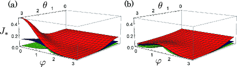
Figure 2: The lower bound $J_{*}(|{\psi}\rangle)$ as a function of $(\theta,\varphi)$ for (a) $\kappa=0$ and (b) $\kappa=1$, in the units of $\gamma=1$. In both cases the curved surface corresponds to $\bar{u}=0,1,5$ from top to bottom.

III.3 Atomic ensemble

Next we study an ensemble composed of $N$ identical atoms. The basic operators for describing this system are the angular momentum operator $J_{i}$ ($i=x,y,z$) satisfying e.g., $[J_{x},J_{y}]=iJ_{z}$, the magnitude ${\bf J}^{2}=J_{x}^{2}+J_{y}^{2}+J_{z}^{2}$, and the ladder operator $J_{-}=J_{x}-iJ_{y}$. Here we focus on the Dicke states $|{l,m}\rangle$, which are the common eigenstates of $J_{z}$ and ${\bf J}^{2}$ defined by $J_{z}|{l,m}\rangle=m|{l,m}\rangle$ and ${\bf J}^{2}|{l,m}\rangle=l(l+1)|{l,m}\rangle$ where $|m|\leq l\leq N/2$ Dicke state Ref Book . Recall, for $N$ even, that $|{N/2,N/2}\rangle$ corresponds to the coherent spin state (CSS) $|{\uparrow}\rangle^{\otimes N}$, i.e., the separable state with all the spins pointing along the $z$ axis, while $|{N/2,0}\rangle$ is highly entangled.

It was proven in Stockton 2004 ; Mirrahimi 2007 that, for the ideal system subjected to the SME (2) with $(H,M,L)=(J_{y},\sqrt{\kappa}J_{z},0)$, the Dicke state $|{N/2,m}\rangle$ for arbitrary $m\in[-N/2,N/2]$ can be deterministically generated by an appropriate MBF control. Now using the lower bound $J_{*}$ we can evaluate how much this MBF control method could work under decoherence. Let $L=\sqrt{\gamma}J_{-}$. Then, the lower bound for $|{\psi}\rangle=|{l,m}\rangle$ is calculated as

$$J_{\ast}=\frac{1}{2}\left[\frac{\gamma(l^{2}+l-m^{2}+m)}{2\kappa m^{2}+2\gamma(l^{2}+l-m^{2})+\bar{u}\sqrt{l^{2}+l-m^{2}}}\right]^{2}.$$

Figure 3(a) shows the case of $N=20$ atoms, for the target Dicke state $|{\psi}\rangle=|{10,m}\rangle$. We observe that, as in the previous studies, the measurement drastically decreases $J_{*}$ especially for the state with large $|m|$, e.g., the CSS $|{10,10}\rangle$. Meanwhile the lower bound at around the entangled state $|{10,0}\rangle$ is almost unaffected by the measurement. Actually in general, for a Dicke state with large $|m|\lesssim l=N/2$, such as the CSS, the measurement term proportional to $\kappa$ is dominant in the denominator of $J_{*}$, while for highly entangled Dicke states with $m\sim 0$ the decoherence term proportional to $\gamma$ becomes dominant. In particular,

$$J_{*}(|{N/2,N/2}\rangle)=\left[\frac{\sqrt{2}\gamma N}{\kappa N^{2}+2\gamma N+\bar{u}\sqrt{2N}}\right]^{2},$$

$$J_{*}(|{N/2,0}\rangle)=\frac{1}{2}\left[\frac{\gamma(N^{2}+2N)}{2\gamma N^{2}+4\gamma N+2\bar{u}\sqrt{N^{2}+2N}}\right]^{2}.$$

Therefore, for a large ensemble limit $N\rightarrow\infty$, we have $J_{*}(|{N/2,N/2}\rangle)\rightarrow 0$ and $J_{*}(|{N/2,0}\rangle)\rightarrow 1/8$. Note that this fundamental bound $J_{*}=1/8$ is applied to all highly entangled Dicke states satisfying $m\sim 0$ and $l\lesssim N/2\gg 1$. That is, while no limitation appears for the case of the CSS thanks to the measurement effect, generating those highly entangled Dicke states is strictly prohibited, irrespective of the use of measurement and control. This result implies that, in practice, there exists a strict limitation in quantum magnetometry that utilizes a highly entangled Dicke state Duan NJP 2014 .

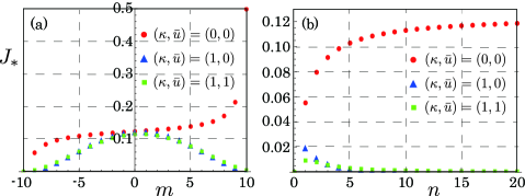
Figure 3: The lower bound $J_{*}$ for (a) the atomic Dicke states and (b) the optical Fock states, in the units of $\gamma=1$.

Another important subject in quantum metrology is the frequency standard, where the GHZ state $|{{\rm GHZ}}\rangle=(|{\uparrow}\rangle^{\otimes N}+|{\downarrow}\rangle^{\otimes N})/\sqrt{2}$ is used for estimating the atomic frequency, over the standard quantum limit attained with the use of the product state $|{+}\rangle^{\otimes N}=(|{\uparrow}\rangle/\sqrt{2}+|{\downarrow}\rangle/\sqrt{2})^{\otimes N}$ Wineland 1996 . The main issue of this technique is that the estimation performance is severely limited Huelga 1997 ; Dorner 2012 due to the dephasing noise, which affects on both the state preparation process and the free-precession process. Here we characterize the performance degradation occurring in the former process, using the lower bound $J_{*}$. In the usual setup where no continuous monitoring is applied, the realistic system obeys the master equation $d\bar{\rho}/dt=-i[H,\bar{\rho}]+\mathcal{D}[L]\bar{\rho}$, where $L=\sqrt{\gamma}J_{z}$ represents the dephasing process and $H$ is a system Hamiltonian representing an open-loop control. Then the lower bounds for the above two states are given by

$$J_{*}(|{+}\rangle^{\otimes N})=\left(\frac{\gamma N}{\sqrt{2}\gamma N+\gamma\sqrt{6N^{2}-4N}+4\,{\mathcal{U}}}\right)^{2},$$

$$J_{\ast}(|{{\rm GHZ}}\rangle)=\left(\frac{\gamma N^{2}}{2\sqrt{2}\gamma N^{2}+4\,{\mathcal{U}}}\right)^{2}.$$

Thus, irrespective of control, $J_{*}(|{+}\rangle^{\otimes N})\rightarrow 1/(8+4\sqrt{3})$ and $J_{*}(|{{\rm GHZ}}\rangle)\rightarrow 1/8$ in the limit $N\to\infty$, under the assumption that ${\mathcal{U}}$ is of the order at most $\sqrt{N}$ and $N$, respectively. Hence, the GHZ state is harder to prepare than the product one, and this gap would erase the quantum advantage obtained using the GHZ state in the ideal setting. In both cases, the estimation performance must be severely limited in the presence of decoherence, if the total time taken for state preparation and free-precession dynamics becomes long; thus, these two processes have to be carried out in as short a time as possible.

III.4 Fock state

The last case study is the problem of generating a Fock state in an optical cavity. In the setup of Geremia 2006 ; Yanagisawa 2006 ; Molmer 2007 , the conditional cavity state obeys the SME (2) with $M=\sqrt{\kappa}a^{\dagger}a$ and $H=i(a^{\dagger}-a)$, where $a$ is the annihilation operator; then it was proven in the ideal case (i.e., $L=0$) that, by choosing an appropriate MBF input $u_{t}$, one can deterministically steer the state to a target Fock state $|{n}\rangle$. Now the lower bound $J_{*}$ can be used to evaluate the performance of this MBF control in the presence of decoherence. A typical decoherence is the photon leakage modeled by $L=\sqrt{\gamma}a$. In this setting, $J_{*}$ for $|{\psi}\rangle=|{n}\rangle$ is calculated as

$$J_{\ast}(|{n}\rangle)=\frac{1}{2}\left[\frac{\gamma n}{2\kappa n^{2}+\gamma(2n+1)+\bar{u}\sqrt{4n+2}}\right]^{2}.$$

Figure 3(b) plots $J_{\ast}$ in the case $\gamma=1$. As in the previous studies, the measurement drastically decreases $J_{*}$. However, $J_{*}\sim 0$ for large Fock states $|{n}\rangle~{}(n\gtrsim 5)$ does not necessarily mean that those states can be exactly stabilized via MBF; rather a large Fock state might be hard to prepare compared to a small one such as $|{1}\rangle$. Hence, in this problem the lower bound only for small Fock states $|{n}\rangle~{}(n\lesssim 4)$ has a practical meaning.

IV Conclusion

In this paper, we have derived the general lower bound $J_{*}$ of the distance between the controlled quantum state under decoherence and an arbitrary target state. The lower bound can be straightforwardly calculated and used as a useful guide for engineering open quantum systems; for instance, in the reservoir engineering scenario, the system should be configured so that $J_{*}$ takes the minimum for a given target state. An important remaining work is to explore an achievable lower bound and develop an efficient method for synthesizing the controller (e.g., the MBF control input) that achieves the bound.

This work was supported in part by JST PRESTO Grant No. JPMJPR166A.

Appendix A Proof of the theorem

We prove the theorem in the MBF setting; the open-loop control and reservoir engineering case is obtained by simply setting the control signal $u_{t}$ to be independent of the conditional state $\rho_{t}$.

First, the infinitesimal change of the random variable

$$j_{t}=1-{\rm Tr}(Q\rho_{t}),~{}~{}~{}Q=|{\psi}\rangle\langle{\psi}|,$$

where $\rho_{t}$ is the solution of the stochastic master equation (2) and $|{\psi}\rangle$ is the target, is given by

$$dj_{t}=-{\rm Tr}(Qd\rho_{t})$$

$$=-{\rm Tr}\big{\{}Q\big{(}-i[u_{t}H,\rho_{t}]dt+\mathcal{D}[L]\rho_{t}dt$$

$$\hskip 10.00002pt\mbox{}+\mathcal{D}[M]\rho_{t}dt+\mathcal{H}[M]\rho_{t}dW_{t}\big{)}\big{\}}$$

$$={\rm Tr}\big{(}iu_{t}[Q,H]\rho_{t}\big{)}dt-{\rm Tr}\big{(}Q\mathcal{D}[L]\rho_{t}\big{)}dt$$

$$\hskip 10.00002pt\hbox{}-{\rm Tr}\big{(}Q\mathcal{D}[M]\rho_{t}\big{)}dt-{\rm Tr}\big{(}Q\mathcal{H}[M]\rho_{t}\big{)}dW_{t}.$$ (7)

The classical stochastic process (the Wiener process) $W_{t}$ satisfies the Ito rule $dW_{t}^{2}=dt$ and $\mathbb{E}(W_{t})=0$. The ensemble average of this equation, with respect to $W_{t}$, is thus

$$\frac{d\mathbb{E}(j_{t})}{dt}={\rm Tr}\big{\{}i[Q,H]\mathbb{E}(u_{t}\rho_{t})\big{\}}-{\rm Tr}\big{\{}Q\mathcal{D}[L]\mathbb{E}(\rho_{t})\big{\}}$$

$$\hskip 30.00005pt\mbox{}-{\rm Tr}\big{\{}Q\mathcal{D}[M]\mathbb{E}(\rho_{t})\big{\}}.$$ (8)

Note again that $u_{t}$ is a function of $\rho_{t}$ in the context of MBF control.

In the proof we often use the Schwarz inequality for matrices (or bounded operators) $X$ and $Y$;

$$\|X\|_{\rm F}\cdot\|Y\|_{\rm F}\geq\frac{1}{2}\Big{|}{\rm Tr}(X^{\dagger}Y+Y^{\dagger}X)\Big{|},$$

where $\|X\|_{\rm F}:=\sqrt{{\rm Tr}(X^{\dagger}X)}$ is the Frobenius norm. In particular, if $X$ and $Y$ are Hermitian, then $\|X\|_{\rm F}\cdot\|Y\|_{\rm F}\geq|{\rm Tr}(XY)|$ holds. The following inequality is also often used:

$$\|\rho_{t}-Q\|_{\rm F}=\sqrt{{\rm Tr}[(\rho_{t}-Q)^{2}]}=\sqrt{{\rm Tr}(\rho_{t}^{2}-2\rho_{t}Q+Q^{2})}$$

$$\hskip 37.00002pt\leq\sqrt{2-2{\rm Tr}(\rho_{t}Q)}=\sqrt{2j_{t}},$$

where ${\rm Tr}(\rho_{t}^{2})\leq 1$ and ${\rm Tr}(Q^{2})={\rm Tr}(Q)=1$ are used.

We begin with calculating a lower bound of the first term on the rightmost side of Eq. (A) as follows:

$${\rm Tr}\big{(}iu_{t}[Q,H]\rho_{t}\big{)} \geq -\bar{u}\Big{|}{\rm Tr}\big{(}i[Q,H]\rho_{t}\big{)}\Big{|}$$

$$= -\bar{u}\Big{|}{\rm Tr}\big{\{}i[Q,H](\rho_{t}-Q)\big{\}}\Big{|}$$

$$\geq -\bar{u}\|i[H,Q]\|_{\rm F}\cdot\|\rho_{t}-Q\|_{\rm F}$$

$$= -\bar{u}\sqrt{{\rm Tr}\{(iHQ-iQH)^{2}\}}\cdot\sqrt{2j_{t}}$$

$$\geq -2\bar{u}\sqrt{\langle{\psi}|H^{2}|{\psi}\rangle-\langle{\psi}|H|{\psi}\rangle^{2}}\cdot\sqrt{j_{t}},$$

where $\bar{u}:=\max\{|u_{t}|\}$ is the upper bound of the control input. Then, by taking the ensemble average of this equation with respect to $W_{t}$, we have

$${\rm Tr}\big{\{}i[Q,H]\mathbb{E}(u_{t}\rho_{t})\big{\}}$$

$$\hskip 30.00005pt\geq-2\bar{u}\sqrt{\langle{\psi}|H^{2}|{\psi}\rangle-\langle{\psi}|H|{\psi}\rangle^{2}}\cdot\mathbb{E}(\sqrt{j_{t}})$$

$$\hskip 30.00005pt\geq-2\bar{u}\sqrt{\langle{\psi}|H^{2}|{\psi}\rangle-\langle{\psi}|H|{\psi}\rangle^{2}}\cdot\sqrt{\mathbb{E}(j_{t})},$$

where $\mathbb{E}(\sqrt{j_{t}})\leq\sqrt{\mathbb{E}(j_{t})}$ is used. Next, the second term on the rightmost side of Eq. (A) can be lower bounded as follows;

$$-{\rm Tr}\big{(}Q\mathcal{D}[L]\rho_{t}\big{)}=-{\rm Tr}\Big{[}Q\big{(}L\rho_{t}L^{\dagger}-\frac{1}{2}\rho_{t}L^{\dagger}L-\frac{1}{2}L^{\dagger}L\rho_{t}\big{)}\Big{]}$$

$$=-{\rm Tr}\big{[}L^{\dagger}QL(\rho_{t}-Q)\big{]}-{\rm Tr}(L^{\dagger}QLQ)+{\rm Tr}(QL^{\dagger}LQ)$$

$$\hskip 10.00002pt\mbox{}-\frac{1}{2}{\rm Tr}\big{[}(Q-\rho_{t})L^{\dagger}LQ+(L^{\dagger}LQ)^{\dagger}(Q-\rho_{t})\big{]}$$

$$\geq-\|L^{\dagger}QL\|_{\rm F}\cdot\|\rho_{t}-Q\|_{\rm F}-\|L^{\dagger}LQ\|_{\rm F}\cdot\|\rho_{t}-Q\|_{\rm F}$$

$$\hskip 10.00002pt\mbox{}+{\rm Tr}(L^{\dagger}LQ)-{\rm Tr}(L^{\dagger}QLQ)$$

$$\geq-\Big{\{}\sqrt{{\rm Tr}\big{[}(L^{\dagger}QL)^{2}\big{]}}+\sqrt{{\rm Tr}\big{[}(L^{\dagger}LQ)^{\dagger}(L^{\dagger}LQ)\big{]}}\Big{\}}\sqrt{2j_{t}}$$

$$\hskip 10.00002pt\mbox{}+{\rm Tr}(L^{\dagger}LQ)-{\rm Tr}(L^{\dagger}QLQ)$$

$$=-\sqrt{2}\left(\langle{\psi}|LL^{\dagger}|{\psi}\rangle+\sqrt{\langle{\psi}|(L^{\dagger}L)^{2}|{\psi}\rangle}\right)\sqrt{j_{t}}$$

$$\hskip 10.00002pt\mbox{}+\langle{\psi}|L^{\dagger}L|{\psi}\rangle-|\langle{\psi}|L|{\psi}\rangle|^{2}$$

$$=-\sqrt{2}\left(\|L^{\dagger}|{\psi}\rangle\|^{2}+\|L^{\dagger}L|{\psi}\rangle\|\right)\sqrt{j_{t}}$$

$$\hskip 10.00002pt\mbox{}+\|L|{\psi}\rangle\|^{2}-|\langle{\psi}|L|{\psi}\rangle|^{2}.$$

Hence again it follows from $\mathbb{E}(\sqrt{j_{t}})\leq\sqrt{\mathbb{E}(j_{t})}$ that

$$-{\rm Tr}\big{\{}Q\mathcal{D}[L]\mathbb{E}(\rho_{t})\big{\}}$$

$$\geq-\sqrt{2}\left(\|L^{\dagger}|{\psi}\rangle\|^{2}+\|L^{\dagger}L|{\psi}\rangle\|\right)\sqrt{\mathbb{E}(j_{t})}$$

$$\hskip 10.00002pt\mbox{}+\|L|{\psi}\rangle\|^{2}-|\langle{\psi}|L|{\psi}\rangle|^{2}.$$

The same inequality as above, with $L$ replaced by $M$, holds. Hence, combining the above three inequalities with Eq. (A) and using the definition $J_{t}=\mathbb{E}(j_{t})=1-{\rm Tr}\big{\{}Q\mathbb{E}(\rho_{t})\big{\}}=1-{\rm Tr}(Q\bar{\rho}_{t})$, we end up with

$$\frac{dJ_{t}}{dt}\geq-\mathcal{U}\sqrt{J_{t}}-\mathcal{A}\sqrt{J_{t}}+\mathcal{E},$$ (9)

where

$$\frac{\mathcal{A}}{\sqrt{2}} = \|L^{\dagger}|{\psi}\rangle\|^{2}+\|L^{\dagger}L|{\psi}\rangle\|+\|M^{\dagger}|{\psi}\rangle\|^{2}+\|M^{\dagger}M|{\psi}\rangle\|,$$

$$\mathcal{U} = 2\bar{u}\sqrt{\langle{\psi}|H^{2}|{\psi}\rangle-\langle{\psi}|H|{\psi}\rangle^{2}},~{}~{}\bar{u}:=\max\{|u_{t}|\},$$

$$\mathcal{E} = \|L|{\psi}\rangle\|^{2}-|\langle{\psi}|L|{\psi}\rangle|^{2}+\|M|{\psi}\rangle\|^{2}-|\langle{\psi}|M|{\psi}\rangle|^{2}.$$

To obtain the lower bound of $J_{t}$ in the limit $t\rightarrow\infty$, let us consider the function $f(x)=-\mathcal{U}\sqrt{x}-\mathcal{A}\sqrt{x}+\mathcal{E}$ in the range $x\in[0,1]$. Clearly, $f(x)$ is a monotonically decreasing function with respect to $x$. Also, from the Schwarz inequality $\|L|{\psi}\rangle\|^{2}-|\langle{\psi}|L|{\psi}\rangle|^{2}\geq 0$, we have $f(0)=\mathcal{E}\geq 0$. Moreover, $f(1)=\mathcal{E}-\mathcal{A}-\mathcal{U}\leq 0$ holds, because

$$\|L|{\psi}\rangle\|^{2} = {\rm Tr}(L^{{\dagger}}LQ)$$

$$= \frac{1}{2}\Big{\{}{\rm Tr}\big{[}(L^{{\dagger}}LQ)^{\dagger}Q\big{]}+{\rm Tr}\big{[}Q^{\dagger}(L^{{\dagger}}LQ)\big{]}\Big{\}}$$

$$\leq \|L^{{\dagger}}LQ\|_{\rm F}\cdot\|Q\|_{\rm F}=\|L^{{\dagger}}LQ\|_{\rm F}=\|L^{\dagger}L|{\psi}\rangle\|,$$

which clearly leads to $\mathcal{E}-\mathcal{A}\leq 0$ and accordingly $\mathcal{E}-\mathcal{A}-\mathcal{U}\leq 0$. In what follows we consider the case ${\mathcal{E}}>0$. Then, from the above properties of $f(x)$, the equation $f(J_{*})=0$ has a unique solution $J_{*}$ in $(0,1]$. Now suppose that $J_{\tau}<J_{*}$ at a given time $\tau$; then Eq. (9) leads to

$$\frac{dJ_{t}}{dt}\Big{|}_{t=\tau} \geq -\mathcal{U}\sqrt{J_{\tau}}-\mathcal{A}\sqrt{J_{\tau}}+\mathcal{E}$$

$$> -\mathcal{U}\sqrt{J_{*}}-\mathcal{A}\sqrt{J_{*}}+\mathcal{E}=0.$$

This means that $J_{t}$ locally increases in time for $t\geq\tau$. Because this argument is true for any $\tau$ such that the inequality $J_{\tau}<J_{*}$ holds, $J_{t}$ increases until $J_{t}$ coincides with $J_{*}$; i.e., $\lim_{t\rightarrow\infty}J_{t}=J_{*}$. On the other hand for the range such that $J_{\tau}\geq J_{*}$ the inequality (9) does not say anything about the local time evolution of $J_{t}$ for $t\geq\tau$. As a result, in the long time limit we have

$$\lim_{t\rightarrow\infty}J_{t}\geq J_{\ast}=\left(\frac{\mathcal{E}}{\mathcal{A}+\mathcal{U}}\right)^{2}.$$

Note that this inequality is valid for the case $\mathcal{E}=0$ as well.

Next we prove that $J_{t}\geq J_{*}$ holds for all $t\in[t_{0},\infty)$, if the initial value $J_{t_{0}}$ is bigger than $J_{*}$. For the proof we use the following fact; see e.g., Diff .

Theorem 2: Consider the following real-valued 1-dimensional ordinary differential equation:

$$\frac{dx(t)}{dt}=f(x(t)),\ \ t\in[t_{0},\infty).$$

If $dx_{1}(t)/dt\leq f(x_{1}(t))$ and $f(x_{2}(t))\leq dx_{2}(t)/dt$, $\forall t\in[t_{0},\infty)$ hold for the initial values satisfying $x_{1}(t_{0})\leq x_{2}(t_{0})$, then $x_{1}(t)\leq x_{2}(t)$ holds for $\forall t\in[t_{0},\infty)$.

Proof: A contradiction argument will be used. Suppose that there exists $t\in[t_{0},\infty)$ such that $x_{1}(t)>x_{2}(t)$. Then, because $x_{1}(t_{0})\leq x_{2}(t_{0})$, there exists $T\geq t_{0}$ satisfying $x_{1}(T)=x_{2}(T)$. Moreover, there exists $h>0$ such that $x_{1}(T+h)>x_{2}(T+h)$ holds. Hence,

$$\frac{dx_{1}(t)}{dt}\Big{|}_{T+0} = \lim_{h\to+0}\frac{x_{1}(T+h)-x_{1}(T)}{h}$$

$$> \lim_{h\to+0}\frac{x_{2}(T+h)-x_{2}(T)}{h}=\frac{dx_{2}(t)}{dt}\Big{|}_{T+0}.$$

Then, from the assumption of Theorem 2,

$$f\left(x_{1}(T)\right)\geq\frac{dx_{1}(t)}{dt}\Big{|}_{T+0}>\frac{dx_{2}(t)}{dt}\Big{|}_{T+0}\geq f\left(x_{2}(T)\right).$$

This is a contradiction to $x_{1}(T)=x_{2}(T)$. Therefore $x_{1}(t)\leq x_{2}(t)$ holds for $\forall t\in[t_{0},\infty)$. $\blacksquare$

Let us apply Theorem 2 to the case $f(x)=-\mathcal{U}\sqrt{x}-\mathcal{A}\sqrt{x}+\mathcal{E}$. Assuming that $x_{1}(t_{0})=J_{*}=\left\{\mathcal{E}/(\mathcal{A}+\mathcal{U})\right\}^{2}$, we have $dx_{1}(t)/dt=f(x_{1}(t))=0$ and $x_{1}(t)=x_{1}(t_{0})=J_{*}$ for $\forall t\in[t_{0},\infty)$. Also we take $x_{2}(t)=J_{t}$, which satisfies the inequality (9), i.e., $dx_{2}(t)/dt\geq f(x_{2}(t))$. Thus, from Theorem 2, if $J_{*}=x_{1}(t_{0})\leq x_{2}(t_{0})=J_{t_{0}}$, then $J_{*}=x_{1}(t)\leq x_{2}(t)=J_{t}$ for all $t\in[t_{0},\infty)$. That is, we obtain

$$J_{t}\geq J_{\ast}=\left(\frac{\mathcal{E}}{\mathcal{A}+\mathcal{U}}\right)^{2},~{}~{}~{}\forall t\in[t_{0},\infty).$$

This is end of the proof of Theorem 1.

Appendix B Generalization of the theorem

If the system dynamics is validly modeled by the stochastic master equation

$$d\rho_{t}= - i\Big{[}\sum_{j}u_{j,t}H_{j},\rho_{t}\Big{]}dt+\sum_{j}\mathcal{D}[L_{j}]\rho_{t}dt$$

$$+ \sum_{j}\mathcal{D}[M_{j}]\rho_{t}dt+\sum_{j}\mathcal{H}[M_{j}]\rho_{t}dW_{t},$$

for the MBF case or the master equation

$$\frac{d\bar{\rho}_{t}}{dt}=-i\Big{[}\sum_{j}u_{j,t}H_{j},\bar{\rho}_{t}\Big{]}+\sum_{j}\mathcal{D}[L_{j}]\bar{\rho}_{t}+\sum_{j}\mathcal{D}[M_{j}]\bar{\rho}_{t},$$

for the open-loop control or reservoir engineering case, by the straightforward extension of the above discussion we find that the lower bound is given by $J_{*}={\mathcal{E}}^{2}/({\mathcal{A}}+{\mathcal{U}})^{2}$ with

$$\mathcal{A} = \sqrt{2}\sum_{j}\left(\|L_{j}^{{\dagger}}|{\psi}\rangle\|^{2}+\|L_{j}^{{\dagger}}L_{j}|{\psi}\rangle\|\right)$$

$$+\sqrt{2}\sum_{j}\left(\|M_{j}^{{\dagger}}|{\psi}\rangle\|^{2}+\|M_{j}^{{\dagger}}M_{j}|{\psi}\rangle\|\right),$$

$$\mathcal{U} = 2\sum_{j}\ \bar{u}_{j}\sqrt{\langle{\psi}|H_{j}^{2}|{\psi}\rangle-\langle{\psi}|H_{j}|{\psi}\rangle^{2}},$$

$$~{}~{}~{}~{}\bar{u}_{j}={\rm max}\{|u_{j,t}|\},$$

$$\mathcal{E} = \sum_{j}\left(\left\|L_{j}|{\psi}\rangle\right\|^{2}-\left|\langle{\psi}|L_{j}|{\psi}\rangle\right|^{2}\right)$$

$$+\sum_{j}\left(\left\|M_{j}|{\psi}\rangle\right\|^{2}-\left|\langle{\psi}|M_{j}|{\psi}\rangle\right|^{2}\right).$$

Using this result we can involve a fixed system Hamiltonian in addition to controllable Hamiltonians; in the simple case where the Hamiltonian is given by $H_{0}+u_{t}H_{1}$ with $H_{0}$ a fixed system Hamiltonian, we have

$${\mathcal{U}} = 2\sqrt{\langle{\psi}|H_{0}^{2}|{\psi}\rangle-\langle{\psi}|H_{0}|{\psi}\rangle^{2}}$$

$$+ 2\bar{u}\sqrt{\langle{\psi}|H_{1}^{2}|{\psi}\rangle-\langle{\psi}|H_{1}|{\psi}\rangle^{2}},$$

with $\bar{u}=\max\{|u_{t}|\}$.

Appendix C A measurement-based feedback control law

Let us consider the continuously-monitored system whose dynamics is given by the following SME:

$$d\rho_{t}=-i[u_{t}J_{y},\rho_{t}]dt+\mathcal{D}[J_{z}]\rho_{t}dt+\mathcal{H}[J_{z}]\rho_{t}dW_{t},$$

where $J_{y}$ and $J_{z}$ are the angular momentum operators. Now the target state $|{\psi}\rangle$ is set to be one of the eigenstates of $J_{z}$. In Ref. Mirrahimi 2007 the authors proposed the following feedback control law that deterministically steers the conditional state $\rho_{t}$ to the target state:

1. $u_{t}=-\alpha{\rm Tr}\left\{i[J_{y},\rho_{t}]Q\right\}$ if ${\rm Tr}(Q\rho_{t})\geq\beta$,

2. $u_{t}=\alpha$ if ${\rm Tr}(Q\rho_{t})\leq\beta/2$,

3. If $\rho_{t}\in\mathcal{B}=\{\rho~{}|~{}\beta/2<{\rm Tr}(Q\rho_{t})<\beta\}$, then $u_{t}=-\alpha{\rm Tr}\left\{i[J_{y},\rho_{t}]Q\right\}$ in the case $\rho_{t}$ last entered $\mathcal{B}$ through the boundary ${\rm Tr}(Q\rho)=\beta$, and $u_{t}=\alpha$ otherwise,

where $\alpha$ and $\beta$ are positive constants. In fact, it was proven that there exists $\beta>0$ such that $\rho_{t}\rightarrow Q=|{\psi}\rangle\langle{\psi}|$ almost surely.

Here we calculate the upper bound $\bar{u}$ of the above MBF control input, in the qubit control problem discussed in Sec. III A. First we have

$${\rm Tr}(\Delta\sigma_{y}^{2}\rho_{t}) = {\rm Tr}(\sigma_{y}^{2}\rho_{t})-[{\rm Tr}(\sigma_{y}\rho_{t})]^{2}$$

$$= 1-[{\rm Tr}(\sigma_{y}\rho_{t})]^{2}\leq 1,$$

$${\rm Tr}(\Delta Q^{2}\rho_{t}) = {\rm Tr}(Q^{2}\rho_{t})-[{\rm Tr}(Q\rho_{t})]^{2}$$

$$= {\rm Tr}(Q\rho_{t})-[{\rm Tr}(Q\rho_{t})]^{2}$$

$$= (1-J_{t})J_{t}\leq\frac{1}{4}.$$

Then, the Robertson inequality ${\rm Tr}(\Delta\sigma_{y}^{2}\rho_{t}){\rm Tr}(\Delta Q^{2}\rho_{t})\geq|{\rm Tr}\{i[\sigma_{y},Q]\rho_{t}\}|^{2}/4$ leads to

$$\Big{|}-\alpha{\rm Tr}\left\{i[J_{y},\rho_{t}]Q\right\}\Big{|} \leq 2\alpha\sqrt{{\rm Tr}(\Delta\sigma_{y}^{2}\rho_{t})}\sqrt{{\rm Tr}(\Delta Q^{2}\rho_{t})}$$

$$\leq 2\alpha\cdot\frac{1}{2}=\alpha.$$

Hence, together with the other case of input, we have $\bar{u}=\max\{|u_{t}|\}=\alpha$; in the numerical simulation depicted in Fig. 1(c) in the main text, $\bar{u}=\alpha=1$ was chosen.

Appendix D Detailed calculations of the lower bound

D.1 Qubit

The target state is $|{\psi}\rangle=[{\rm cos}\theta,\ e^{i\varphi}{\rm sin}\theta]^{\top}$ $(0\leq\theta<\pi/2,0\leq\varphi<2\pi)$, and the system operators are $H=\sigma_{y}$, $M=\sqrt{\kappa}\sigma_{z}$, and $L=\sqrt{\gamma}\sigma_{-}$. Then we have

$$\frac{\mathcal{A}}{\sqrt{2}} = \|L^{\dagger}|{\psi}\rangle\|^{2}+\|L^{\dagger}L|{\psi}\rangle\|+\|M^{\dagger}|{\psi}\rangle\|^{2}+\|M^{\dagger}M|{\psi}\rangle\|$$

$$= 2\kappa+\gamma\sin^{2}\theta+\gamma\cos\theta,$$

$$\mathcal{U} = 2\bar{u}\sqrt{\langle{\psi}|H^{2}|{\psi}\rangle-\langle{\psi}|H|{\psi}\rangle^{2}}$$

$$= 2\bar{u}\sqrt{1-\sin^{2}2\theta\sin^{2}\varphi},$$

$$\mathcal{E} = \|L|{\psi}\rangle\|^{2}-|\langle{\psi}|L|{\psi}\rangle|^{2}+\|M|{\psi}\rangle\|^{2}-|\langle{\psi}|M|{\psi}\rangle|^{2}$$

$$= \kappa\sin^{2}2\theta+\gamma\cos^{4}\theta.$$

D.2 Qutrit

The target state is limited to the real vector $|{\psi}\rangle=[\sin(\theta/2)\cos(\varphi/2),\,\cos(\theta/2),\,\sin(\theta/2)\sin(\varphi/2)]^{\top}$. The system operators are given by

$$H = \frac{1}{\sqrt{2}}\left[\begin{array}[]{rrr}0&-i&0\\ i&0&-i\\ 0&i&0\end{array}\right],\ M=\sqrt{\kappa}\left[\begin{array}[]{rrr}1&0&0\\ 0&0&0\\ 0&0&-1\end{array}\right],$$

$$L = \sqrt{\gamma}\left[\begin{array}[]{rrr}0&0&0\\ 1&0&0\\ 0&1&0\end{array}\right].$$

Then, from the definition of ${\mathcal{A}}$, ${\mathcal{U}}$, and ${\mathcal{E}}$, we have

$$\frac{{\mathcal{A}}}{\sqrt{2}}=\kappa\left({\rm sin}^{2}\frac{\theta}{2}+{\rm sin}\frac{\theta}{2}\right)$$

$$\mbox{}+\gamma\left({\rm cos}^{2}\frac{\theta}{2}+{\rm sin}^{2}\frac{\theta}{2}{\rm sin}^{2}\frac{\varphi}{2}+\sqrt{{\rm sin}^{2}\frac{\theta}{2}{\rm cos}^{2}\frac{\varphi}{2}+{\rm cos}^{2}\frac{\theta}{2}}\right),$$

$$\mathcal{U}=\sqrt{2}\bar{u}\sqrt{1+{\rm cos}^{2}\frac{\theta}{2}-{\rm sin}^{2}\frac{\theta}{2}{\rm sin}\varphi},$$

$$\mathcal{E}=\kappa\left({\rm sin}^{2}\frac{\theta}{2}+{\rm sin}\frac{\theta}{2}\right)$$

$$\mbox{}+\gamma\left({\rm sin}^{2}\frac{\theta}{2}{\rm sin}^{2}\frac{\varphi}{2}+{\rm cos}^{2}\frac{\theta}{2}+\sqrt{{\rm sin}^{2}\frac{\theta}{2}{\rm cos}^{2}\frac{\varphi}{2}+{\rm cos}\frac{\theta}{2}}\right).$$

D.3 Dicke state

The target is the Dicke state $|{l,m}\rangle$, and the system operators are $H=J_{y}$, $M=\sqrt{\kappa}J_{z}$, and $L=\sqrt{\gamma}J_{-}$. Recall that $|{l,m}\rangle$ is a common eigenvector of $J_{z}$ and the orbital angular momentum operator ${\bf J}^{2}=J_{x}^{2}+J_{y}^{2}+J_{z}^{2}$;

$$J_{z}|{l,m}\rangle=m|{l,m}\rangle,~{}~{}{\bf J}^{2}|{l,m}\rangle=l(l+1)|{l,m}\rangle.$$

Also the raising and lowering operators $J_{\pm}=J_{x}\pm iJ_{y}$ act on $|{l,m}\rangle$ as follows:

$$J_{\pm}|{l,m}\rangle=\sqrt{(l\mp m)(l\pm m+1)}|{l,m\pm 1}\rangle.$$

The following equations are also used;

$$J_{+}J_{-} = (J_{x}+iJ_{y})(J_{x}-iJ_{y})$$

$$= J_{x}^{2}+J_{y}^{2}-iJ_{x}J_{y}+iJ_{y}J_{x}$$

$$= {\bf J}^{2}-J_{z}^{2}-i[J_{x},J_{y}]={\bf J}^{2}-J_{z}^{2}+J_{z},$$

and likewise $J_{-}J_{+}={\bf J}^{2}-J_{z}^{2}-J_{z}$. Then we have

$$\mathcal{A}=\sqrt{2}\Big{(}\kappa\|J_{z}|{l,m}\rangle\|^{2}+\kappa\|J^{2}_{z}|{l,m}\rangle\|$$

$$\hskip 20.00003pt\mbox{}+\gamma\|J_{-}^{{\dagger}}|{l,m}\rangle\|^{2}+\gamma\|J_{-}^{{\dagger}}J_{-}|{l,m}\rangle\|\Big{)}$$

$$=\sqrt{2}\Big{[}\kappa m^{2}+\kappa m^{2}+\gamma\{l(l+1)-m^{2}-m\}$$

$$\hskip 20.00003pt\mbox{}+\gamma\{l(l+1)-m^{2}+m\}\Big{]}$$

$$=\sqrt{2}\left\{2\kappa m^{2}+2\gamma(l^{2}+l-m^{2})\right\},$$

$$\mathcal{U}=\bar{u}\sqrt{\left\|(J_{-}^{{\dagger}}-J_{-})|{l,m}\rangle\right\|^{2}-\left|\langle{l,m}|(J_{-}^{{\dagger}}-J_{-})|{l,m}\rangle\right|^{2}}$$

$$=\bar{u}\sqrt{\left\{(l-m)(l+m+1)+(l+m)(l-m+1)\right\}}$$

$$=\sqrt{2}\bar{u}\sqrt{l^{2}+l-m^{2}},$$

$$\mathcal{E}=\kappa\|J_{z}|{l,m}\rangle\|^{2}-\kappa\left|\langle{l,m}|J_{z}|{l,m}\rangle\right|^{2}$$

$$\hskip 20.00003pt\mbox{}+\gamma\|J_{-}|{l,m}\rangle\|^{2}-\gamma\left|\langle{l,m}|J_{-}|{l,m}\rangle\right|^{2}$$

$$=\kappa m^{2}-\kappa m^{2}+\gamma(l+m)(l-m+1)$$

$$=\gamma(l^{2}+l-m^{2}+m).$$

D.4 Product state of the spin superposition

The target is the product state of the spin superposition, $|{+}\rangle^{\otimes N}$, where $|{+}\rangle=(|{\uparrow}\rangle+|{\downarrow}\rangle)/\sqrt{2}$. The system is driven by the dephasing process $L=\sqrt{\gamma}J_{z}$ and an appropriate control Hamiltonian $H$, but it is not subjected to continuous monitoring and subsequent MBF (i.e., $M=0$). Recall that $J_{z}$ can be represented as

$$J_{z}=\frac{1}{2}\sum^{N}_{j=1}\sigma^{(j)}_{z}=\frac{1}{2}\sum^{N}_{j=1}(I\otimes\cdots\otimes\sigma_{z}\otimes\cdots\otimes I),$$ (12)

where the Pauli matrix $\sigma_{z}$ appears in the $j$th component. $\sigma_{z}$ acts on $|{\uparrow}\rangle$ and $|{\downarrow}\rangle$ as $\sigma_{z}|{\uparrow}\rangle=|{\uparrow}\rangle$ and $\sigma_{z}|{\downarrow}\rangle=-|{\downarrow}\rangle$, respectively. Hence we have $\sigma_{z}|{+}\rangle=|{-}\rangle$, where $|{-}\rangle=(|{\uparrow}\rangle-|{\downarrow}\rangle)/\sqrt{2}$. Moreover,

$$L|{+}\rangle^{\otimes N}=\frac{\sqrt{\gamma}}{2}\sum^{N}_{j=1}|{+}\rangle\cdots|{+}\rangle|{-}\rangle|{+}\rangle\cdots|{+}\rangle$$

holds, where $|{-}\rangle$ appears in the $j$th component. This leads to $\langle{+}|^{\otimes N}L|{+}\rangle^{\otimes N}=0$ and thus

$$\mathcal{E}=\left\|L|{+}\rangle^{\otimes N}\right\|^{2}-\left|\langle{+}|^{\otimes N}L|{+}\rangle^{\otimes N}\right|^{2}=\frac{\gamma N}{4}.$$

Also, we have

$$L^{\dagger}L|{+}\rangle^{\otimes N}$$

$$=\frac{\gamma}{4}\Big{(}N|{+}\rangle^{\otimes N}+2\sum_{i\neq j}|{+}\rangle\ldots|{-}\rangle\cdots|{-}\rangle\ldots|{+}\rangle\Big{)},$$

where $|{-}\rangle$ appears only in the $i$th and $j$th components ($i\neq j$). Hence,

$$\mathcal{A} = \sqrt{2}\left(\left\|L^{{\dagger}}|{+}\rangle^{\otimes N}\right\|^{2}+\left\|L^{{\dagger}}L|{+}\rangle^{\otimes N}\right\|\right)$$

$$= \frac{\gamma}{4}\Big{(}\sqrt{2}N+\sqrt{6N^{2}-4N}\Big{)}.$$

D.5 GHZ state

The target is $|{{\rm GHZ}}\rangle=\left(|{\uparrow}\rangle^{\otimes N}+|{\downarrow}\rangle^{\otimes N}\right)/\sqrt{2}$. As in the previous case, the system is driven by the dephasing process $L=\sqrt{\gamma}J_{z}$ and an appropriate Hamiltonian $H$, while not subjected to MBF (i.e., $M=0$). Using the representation (12) we have

$$\frac{\mathcal{A}}{\sqrt{2}}=\left\|L^{{\dagger}}|{{\rm GHZ}}\rangle\right\|^{2}+\left\|L^{{\dagger}}L|{{\rm GHZ}}\rangle\right\|$$

$$=\frac{\gamma}{8}N^{2}\left\||{\uparrow}\rangle^{\otimes N}-|{\downarrow}\rangle^{\otimes N}\right\|^{2}+\frac{\gamma}{4\sqrt{2}}N^{2}\left\||{\uparrow}\rangle^{\otimes N}+|{\downarrow}\rangle^{\otimes N}\right\|$$

$$=\frac{\gamma}{4}N^{2}+\frac{\gamma}{4}N^{2}=\frac{\gamma}{2}N^{2},$$

$$\mathcal{E}=\left\|L|{{\rm GHZ}}\rangle\right\|^{2}-\left|\langle{{\rm GHZ}}|L|{{\rm GHZ}}\rangle\right|^{2}$$

$$=\frac{\gamma}{8}N^{2}\left\||{\uparrow}\rangle^{\otimes N}-|{\downarrow}\rangle^{\otimes N}\right\|^{2}-0=\frac{\gamma}{4}N^{2}.$$

D.6 Fock State

The target is an arbitrary Fock state $|{n}\rangle$ and the system operators are given by $H=i(a^{{\dagger}}-a)$, $M=\sqrt{\kappa}a^{{\dagger}}a$, and $L=\sqrt{\gamma}a$. Using $a|{n}\rangle=\sqrt{n}|{n-1}\rangle$ and $a^{{\dagger}}|{n}\rangle=\sqrt{n+1}|{n+1}\rangle$, we have

$$\mathcal{A}=\sqrt{2}\Big{(}\kappa\left\|a^{{\dagger}}a|{n}\rangle\right\|^{2}+\kappa\left\|a^{{\dagger}}aa^{{\dagger}}a|{n}\rangle\right\|$$

$$\hskip 30.00005pt\mbox{}+\gamma\left\|a^{{\dagger}}|{n}\rangle\right\|^{2}+\gamma\left\|a^{{\dagger}}a|{n}\rangle\right\|\Big{)}$$

$$=2\sqrt{2}\kappa n^{2}+\sqrt{2}\gamma(2n+1),$$

$$\mathcal{U}=2\bar{u}\sqrt{\left\|i(a^{{\dagger}}-a)|{n}\rangle\right\|^{2}-\langle{n}|i(a^{{\dagger}}-a)|{n}\rangle^{2}}$$

$$=2\bar{u}\sqrt{2n+1},$$

$$\mathcal{E}=\kappa\left\|a^{{\dagger}}a|{n}\rangle\right\|^{2}-\kappa\left|\langle{n}|a^{{\dagger}}a|{n}\rangle\right|^{2}$$

$$\hskip 30.00005pt\mbox{}+\gamma\left\|a|{n}\rangle\right\|^{2}-\gamma\left|\langle{n}|a|{n}\rangle\right|^{2}$$

$$=\gamma n.$$

References

- (1) W. S. Warren, H. Rabitz, and M. Dahleh, Coherent control of quantum dynamics: The dream is alive, Science 259, 1581 (1993).
- (2) L. Viola, E. Knill, and S. Lloyd, Dynamical decoupling of open quantum systems, Phys. Rev. Lett. 82, 2417 (1999).
- (3) N. Khaneja, T. Reiss, B. Luy, and S. J. Glaser, Optimal control of spin dynamics in the presence of relaxation, J. Magn. Reson. 162, 311 (2003).
- (4) D. D’Alessandro, Introduction to Quantum Control and Dynamics (Chapman Hall/CRC, 2007).
- (5) K. Jacobs, Engineering quantum states of a nanoresonator via a simple auxiliary system, Phys. Rev. Lett. 99, 117203 (2007).
- (6) K. Jacobs, L. Tian, and J. Finn, Engineering superposition states and tailored probes for nanoresonators via open-loop control, Phys. Rev. Lett. 102, 057208 (2009).
- (7) P. Doria, T. Calarco, and S. Montangero, Optimal control technique for many-body quantum dynamics Phys. Rev. Lett. 106, 190501 (2011).
- (8) J. Li, D. Lu, Z. Luo, R. Laflamme, X. Peng, and J. Du, Approximation of reachable set for coherently controlled open quantum systems: Application to quantum state engineering, Phys. Rev. A 94, 012312 (2016).
- (9) J. K. Stockton, R. van Handel, and H. Mabuchi, Deterministic Dicke-state preparation with continuous measurement and control, Phys. Rev. A 70, 022106 (2004).
- (10) R. van Handel, J. K. Stockton, and H. Mabuchi, Feedback contorol of quantum state reduction, IEEE Trans. Automat. Contr. 50-6, 768/780 (2005).
- (11) JM. Geremia, Deterministic and nondestructively verifiable preparation of photon number states, Phys. Rev. Lett. 97, 073601 (2006).
- (12) M. Yanagisawa, Quantum feedback control for deterministic entangled photon generation, Phys. Rev. Lett. 97, 190201 (2006).
- (13) N. Yamamoto, K. Tsumura, and S. Hara, Feedback control of quantum entanglement in a two-spin system, Automatica 43-6, 981/992 (2007).
- (14) A. Negretti, U. V. Poulsen, and K. Molmer, Quantum superposition state production by continuous observations and feedback, Phys. Rev. Lett. 99, 223601 (2007).
- (15) M. Mirrahimi and R. van Handel, Stabilizing feedback controls for quantum systems, SIAM J. Control Optim. 46-2, 445/467 (2007).
- (16) L. Bouten, R. van Handel, and M. R. James, A discrete invitation to quantum filtering and feedback control, SIAM Review 51, 239-316 (2009).
- (17) J. F. Poyatos, J. I. Cirac, and P. Zoller, Quantum reservoir engineering with laser cooled trapped ions, Phys. Rev. Lett. 77, 4728 (1996).
- (18) S. G. Schirmer and X. Wang Stabilizing open quantum systems by Markovian reservoir engineering, Phys. Rev. A 81, 062306 (2010).
- (19) N. Yamamoto, Coherent versus measurement feedback: Linear systems theory for quantum information, Phys. Rev. X 4, 041029 (2014).
- (20) M. Asjad and D. Vitali, Reservoir engineering of a mechanical resonator: generating a macroscopic superposition state and monitoring its decoherence, J. Phys. B: At. Mol. Opt. Phys. 47, 045502 (2014).
- (21) J.-R. Souquet and A. A. Clerk, Fock-state stabilization and emission in superconducting circuits using dc-biased Josephson junctions, Phys. Rev. A 93, 060301 (2016).
- (22) J. Combes, J. Kerckhoff, and M. Sarovar, The SLH framework for modeling quantum input-output networks, Advances in Physics: X 2-3, 784/888 (2017).
- (23) M. Brunelli, O. Houhou, D. W. Moore, A. Nunnenkamp, M. Paternostro, and A. Ferraro, Unconditional preparation of nonclassical states via linear-and-quadratic optomechanics, Phys. Rev. A 98, 063801 (2018).
- (24) C. Sayrin, et al., Real-time quantum feedback prepares and stabilizes photon number states. Nature 477, 73 (2011).
- (25) R. Vijay, et al., Stabilizing Rabi oscillations in a superconducting qubit using quantum feedback, Nature 490, 77 (2012).
- (26) D. Riste, et al., Deterministic entanglement of superconducting qubits by parity measurement and feedback, Nature 502, 350 (2013).
- (27) S. Hacohen-Gourgy, et al., Quantum dynamics of simultaneously measured non-commuting observables, Nature 538, 491 (2016).
- (28) K. C. Cox, G. P. Greve, J. M. Weiner, and J. K. Thompson, Deterministic squeezed states with collective measurements and feedback, Phys. Rev. Lett. 116, 093602 (2016).
- (29) Y. Liu, et al., Comparing and combining measurement-based and driven-dissipative entanglement stabilization, Phys. Rev. X 6, 011022 (2016).
- (30) S. Lloyd and S. Montangero, Information theoretical analysis of quantum optimal control, Phys. Rev. Lett. 113, 010502 (2014).
- (31) C. P. Koch, Controlling open quantum systems: tools, achievements, and limitations, J. Phys.: Condens. Matter 28 213001 (2016).
- (32) N. Khaneja, B. Luy, and S. J. Glaser, Boundary of quantum evolution under decoherence, PNAS 100-23, 13162/13166 (2003).
- (33) B. Qi and L. Guo, Is measurement-based feedback still better for quantum control systems?, System and Control Letters 59-6, 333/339 (2010).
- (34) B. Qi, H. Pan, and L. Guo, Further results on stabilizing control of quantum systems, IEEE Trans. Automat. Contr. 58-5 1349/1354 (2013).
- (35) C. Altafini, Controllability properties for finite dimensional quantum Markovian master equations, J. Math. Phys. 44-6, 2357/2372 (2003).
- (36) J. S. Li and N. Khaneja, Ensemble control of Bloch equations, IEEE Trans. Automat. Contr. 54-3, 528/536 (2009).
- (37) G. Dirr, U. Helmke, I. Kurniawan, and T. Schulte-Herbruggen, Lie-semigroup structures for reachability and control of open quantum systems: Kossakowski-Lindblad generators form Lie-wedge to Markovian channels, Reports Math. Phys. 64, 93/121 (2009).
- (38) I. Kurniawan, G. Dirr, and U. Helmke, Controllability aspects of quantum dynamics: A unified approach for closed and open systems, IEEE Trans. Automat. Contr. 57-8, 1984/1996 (2012).
- (39) C. O’Meara, G. Dirr, and T. Schulte-Herbruggen, Illustrating the geometry of coherently controlled unital open quantum systems, IEEE Trans. Automat. Contr. 57-8, 2050/2056 (2012).
- (40) H. Yuan, Reachable set of open quantum dynamics for a single spin in Markovian environment, Automatica 49-4, 955/959 (2013).
- (41) H. M. Wiseman and G. J. Milburn, Quantum Measurement and Control (Cambridge University Press, 2010).
- (42) K. Jacobs, Quantum Measurement Theory and its Applications (Cambridge Univ. Press, 2014).
- (43) H. I. Nurdin and N. Yamamoto, Linear Dynamical Quantum Systems: Analysis, Synthesis, and Control (Springer, 2017).
- (44) M. A. Nielsen and I. L. Chuang, Quantum Computation and Quantum information (Cambridge University Press, 2010).
- (45) R. Bianchetti, et al., Control and tomography of a three level superconducting artificial atom, Phys. Rev. Lett. 105, 223601 (2010).
- (46) L. Mandel and E. Wolf, Optical Coherence and Quantum Optics (Cambridge University Press, Cambridge, UK, 1997).
- (47) Z. Zhang and L. M. Duan, Quantum metrology with Dicke squeezed states, New J. Phys. 16, 103037 (2014).
- (48) J. J . Bollinger, W. M. Itano, D. J. Wineland, and D. J. Heinzen, Optimal frequency measurements with maximally correlated states, Phys. Rev. A 54, 4649 (1996).
- (49) S. F. Huelga, C. Macchiavello, T. Pellizzari, A. K. Ekert, M. B. Plenio, and J. I. Cirac, Improvement of frequency standards with quantum entanglement, Phys. Rev. Lett. 79, 3865 (1997).
- (50) U. Dorner, Quantum frequency estimation with trapped ions and atoms, New J. Phys. 14, 043011 (2012).
- (51) R. P. Agarwal and D. O’Regan, An introduction to ordinary differential equations (Springer, 2008).