Fast mixing of Metropolized Hamiltonian Monte Carlo: Benefits of multi-step gradients

Abstract

Hamiltonian Monte Carlo (HMC) is a state-of-the-art Markov chain Monte Carlo sampling algorithm for drawing samples from smooth probability densities over continuous spaces. We study the variant most widely used in practice, Metropolized HMC with the Störmer-Verlet or leapfrog integrator, and make two primary contributions. First, we provide a non-asymptotic upper bound on the mixing time of the Metropolized HMC with explicit choices of step-size and number of leapfrog steps. This bound gives a precise quantification of the faster convergence of Metropolized HMC relative to simpler MCMC algorithms such as the Metropolized random walk, or Metropolized Langevin algorithm. Second, we provide a general framework for sharpening mixing time bounds of Markov chains initialized at a substantial distance from the target distribution over continuous spaces. We apply this sharpening device to the Metropolized random walk and Langevin algorithms, thereby obtaining improved mixing time bounds from a non-warm initial distribution.

1 Introduction

Markov Chain Monte Carlo (MCMC) methods date back to the seminal work of Metropolis et al. (1953), and are the method of choice for drawing samples from high-dimensional distributions. They are widely used in practice, including in Bayesian statistics for exploring posterior distributions (Carpenter et al., 2017; Smith, 2014), in simulation-based methods for reinforcement learning, and in image synthesis in computer vision, among other areas. Since their origins in the 1950s, many MCMC algorithms have been introduced, applied and studied; we refer the reader to the handbook by Brooks et al. (2011) for a survey of known results and contemporary developments.

There are a variety of MCMC methods for sampling from target distributions with smooth densities (Robert and Casella, 1999; Roberts et al., 2004; Roberts and Stramer, 2002; Brooks et al., 2011). Among them, the method of Hamiltonian Monte Carlo (HMC) stands out among practitioners: it is the default sampler for sampling from complex distributions in many popular software packages, including Stan (Carpenter et al., 2017), Mamba (Smith, 2014), and Tensorflow (Abadi et al., 2015). We refer the reader to the papers (Neal, 2011; Hoffman and Gelman, 2014; Durmus et al., 2017) for further examples and discussion of the HMC method. There are a number of variants of HMC, but the most popular choice involves a combination of the leapfrog integrator with Metropolis-Hastings correction. Throughout this paper, we reserve the terminology HMC to refer to this particular Metropolized algorithm. The idea of using Hamiltonian dynamics in simulation first appeared in Alder and Wainwright (1959). Duane et al. (1987) introduced MCMC with Hamiltonian dynamics, and referred to it as Hybrid Monte Carlo. The algorithm was further refined by Neal (1994), and later re-christened in the statistics community as Hamiltonian Monte Carlo. We refer the reader to Neal (2011) for an illuminating overview of the history of HMC and a discussion of contemporary work.

1.1 Past work on HMC

While HMC enjoys fast convergence in practice, a theoretical understanding of this behavior remains incomplete. Some intuitive explanations are based on its ability to maintain a constant asymptotic accept-reject rate with large step-size (Creutz, 1988). Others suggest, based on intuition from the continuous-time limit of the Hamiltonian dynamics, that HMC can suppress random walk behavior using momentum (Neal, 2011). However, these intuitive arguments do not provide rigorous or quantitative justification for the fast convergence of the discrete-time HMC used in practice.

More recently, general asymptotic conditions under which HMC will or will not be geometrically ergodic have been established in some recent papers (Durmus et al., 2017; Livingstone et al., 2016). Other work has yielded some insight into the mixing properties of different variants of HMC, but it has focused mainly on unadjusted versions of the algorithm. Mangoubi and Smith (2017) and Mangoubi and Vishnoi (2018) study versions of unadjusted HMC based on Euler discretization or leapfrog integrator (but omitting the Metropolis-Hastings step), and provide explicit bounds on the mixing time as a function of dimension $d$, condition number $\kappa$ and error tolerance $\epsilon>0$. Lee et al. (2018) studied an extended version of HMC that involves applying an ordinary differential equation (ODE) solver; they established bounds with sublinear dimension dependence, and even polylogarithmic for certain densities (e.g., those arising in Bayesian logistic regression). The mixing time for the same algorithm is further refined in recent work by Chen and Vempala (2019). In a similar spirit, Lee and Vempala (2018a) studied the Riemannian variant of HMC (RHMC) with an ODE solver focusing on sampling uniformly from a polytope. While their result could be extended to log-concave sampling, the practical implementation of their ODE solver for log-concave sampling is unclear. Moreover, it requires a regularity condition on all the derivatives of density. One should note that such unadjusted HMC methods behave differently from the Metropolized version most commonly used in practice. In the absence of the Metropolis-Hastings correction, the resulting Markov chain no longer converges to the correct target distribution, but instead exhibits a persistent bias, even in the limit of infinite iterations. Consequently, the analysis of such sampling methods requires controlling this bias; doing so leads to mixing times that scale polynomially in $1/\epsilon$, in sharp contrast with the $\log(1/\epsilon)$ that is typical for Metropolis-Hastings corrected methods.

Most closely related to our paper is the recent work by Bou-Rabee et al. (2018), which studies the same Metropolized HMC algorithm that we analyze in this paper. They use coupling methods to analyze HMC for a class of distributions that are strongly log-concave outside of a compact set. In the strongly log-concave case, they prove a mixing-time bound that scales at least as $d^{3/2}$ in the dimension $d$. We note that with a “warm” initialization, this dimension dependence grows more quickly than known bounds for the MALA algorithm (Dwivedi et al., 2019; Eberle, 2014), and so does not explain the superiority of HMC in practice.

In practice, it is known that Metropolized HMC is fairly sensitive to the choice of its parameters—namely the step-size $\eta$ used in the discretization scheme, and the number of leapfrog steps $K$. At one extreme, taking a single leapfrog step $K=1$, the algorithm reduces to the Metropolis adjusted Langevin algorithm (MALA). More generally, if too few leapfrog steps are taken, HMC is likely to exhibit a random walk behavior similar to that of MALA. At the other extreme, if $K$ is too large, the leapfrog steps tend to wander back to a neighborhood of the initial state, which leads to wasted computation as well as slower mixing (Betancourt et al., 2014). In terms of the step size $\eta$, when overly large step size is chosen, the discretization diverges from the underlying continuous dynamics leading to a drop in the Metropolis acceptance probability, thereby slowing down the mixing of the algorithm. On the other hand, an overly small choice of $\eta$ does not allow the algorithm to explore the state space rapidly enough. While it is difficult to characterize the necessary and sufficient conditions on $K$ and $\eta$ to ensure fast convergence, many works suggest the choice of these two parameters based on the necessary conditions such as maintaining a constant acceptance rate (Chen et al., 2001). For instance, Beskos et al. (2013) showed that in the simplified scenario of target density with independent, identically distributed components, the number of leapfrog steps should scale as $d^{1/4}$ to achieve a constant acceptance rate. Besides, instead of setting the two parameters explicitly, various automatic strategies for tuning these two parameters have been proposed (Wang et al., 2013; Hoffman and Gelman, 2014; Wu et al., 2018). Despite being introduced via heuristic arguments and with additional computational cost, these methods, such as the No-U-Turn (NUTS) sampler (Hoffman and Gelman, 2014), have shown promising empirical evidence of its effectiveness on a wide range of simple target distributions.

1.2 Past work on mixing time dependency on initialization

Many proof techniques for the convergence of continuous-state Markov chains are inspired by the large body of work on discrete-state Markov chains; for instance, see the surveys (Lovász et al., 1993; Aldous and Fill, 2002) and references therein. Historically, much work has been devoted to improving the mixing time dependency on the initial distribution. For discrete-state Markov chains, Diaconis and Saloff-Coste (1996) were the first to show that the logarithmic dependency of the mixing time of a Markov chain on the warmness parameter of the starting distribution can be improved to doubly logarithmic. This improvement—from logarithmic to doubly logarithmic—allows for a good bound on the mixing time even when a good starting distribution is not available. The innovation underlying this improvement is the use of log-Sobolev inequalities in place of the usual isoperimetric inequality. Later, closely related ideas such as average conductance (Lovász and Kannan, 1999; Kannan et al., 2006), evolving sets (Morris and Peres, 2005) and spectral profile (Goel et al., 2006) were shown to be effective for reducing dependence on initial conditions for discrete space chains. Thus far, only the notion of average conductance (Lovász and Kannan, 1999; Kannan et al., 2006) has been adapted to continuous-state Markov chains so as to sharpen the mixing time analysis of the Ball walk (Lovász and Simonovits, 1990).

1.3 Our contributions

This paper makes two primary contributions. First, we provide a non-asymptotic upper bound on the mixing time of the Metropolized HMC algorithm for smooth densities (see Theorem 1). This theorem applies to the form of Metropolized HMC (based on the leapfrog integrator) that is most widely used in practice. To the best of our knowledge, Theorem 1 is the first rigorous confirmation of the faster non-asymptotic convergence of the Metropolized HMC as compared to MALA and other simpler Metropolized algorithms. Other related works on HMC consider either its unadjusted version (without accept-reject step) with different integrators (Mangoubi and Smith, 2017; Mangoubi and Vishnoi, 2018) or the HMC based on an ODE solver (Lee et al., 2018; Lee and Vempala, 2018a). While the dimension dependency for these algorithms is usually better than MALA, they have polynomial dependence on the inverse error tolerance $1/\epsilon$ while MALA’s mixing time scales as $\log(1/\epsilon)$. Moreover, our direct analysis of the Metropolized HMC with a leapfrog integrator provides explicit choices of the hyper-parameters for the sampler, namely, the step-size and the number of leapfrog updates in each step. Our theoretical choices of the hyper-parameters could potentially provide guidelines for parameter tuning in practical HMC implementations

Our second main contribution is formalized in Lemmas 3 and 4: we develop results based on the conductance profile in order to prove quantitative convergence guarantees general continuous-state space Markov chains. Doing so involves non-trivial extensions of ideas from discrete-state Markov chains to those in continuous state spaces. Our results not only enable us to establish the mixing time bounds for HMC with different classes of target distributions, but also allow simultaneous improvements on mixing time bounds of several Markov chains (for general continuous-state space) when the starting distribution is far from the stationary distribution. Consequentially, we improve upon previous mixing time bounds for Metropolized Random Walk (MRW) and MALA (Dwivedi et al., 2019), when the starting distribution is not warm with respect to the target distribution (see Theorem 5).

While this high-level road map is clear, a number of technical challenges arise en route in particular in controlling the conductance profile of HMC. The use of multiple gradient steps in each iteration of HMC helps it mix faster but also complicates the analysis; in particular, a key step is to control the overlap between the transition distributions of HMC chain at two nearby points; doing so requires a delicate argument (see Lemma 6 and Section 5.3 for further details).

Table 1 provides an informal summary of our mixing time bounds of HMC and how they compare with known bounds for MALA when applied to log-concave target distributions. From the table, we see that Metropolized HMC takes fewer gradient evaluations than MALA to mix to the same accuracy for log-concave distributions. Note that our current analysis establishes logarithmic dependence on the target error $\epsilon$ for strongly-log-concave as well as for a sub-class of weakly log-concave distributions. Moreover, in Figure 1 we provide a sketch-diagram of how the different results in this paper interact to provide mixing time bounds for different Markov chains.

	Strongly log-concave	Weakly log-concave
Sampling algorithm	Assumption (B) ($\kappa\ll d$)	Assumption (C)	Assumption (D)
MALA (improved bound in Thm 5 in this paper)	$\displaystyle d\kappa\log\frac{1}{\epsilon}$ Dwivedi et al. (2019)	$\displaystyle\frac{d^{2}}{\epsilon^{\frac{3}{2}}}\log\frac{1}{\epsilon}$ Dwivedi et al. (2019)	$\displaystyle d^{\frac{3}{2}}\log\frac{1}{\epsilon}$ Mangoubi and Vishnoi (2019)
Metropolized HMC with leapfrog integrator  [this paper]	$\displaystyle d^{\frac{11}{12}}\kappa\log\frac{1}{\epsilon}$ (Corollary 2)	$\displaystyle\frac{d^{\frac{11}{6}}}{\epsilon}\log\frac{1}{\epsilon}$ (Corollary 18)	$\displaystyle d^{\frac{4}{3}}\log\frac{1}{\epsilon}$ (Corollary 18)

Table 1: Comparisons of the number of gradient evaluations needed by MALA and Metropolized HMC with leapfrog integrator from a warm start to obtain an $\epsilon$-accurate sample in TV distance from a log-concave target distribution on ^d. The second column corresponds to strongly log-concave densities with condition number $\kappa$, and the third and fourth column correspond to weakly log-concave densities satisfying certain regularity conditions.

Figure 1: High-level sketch diagram of the results and the proof techniques developed in this paper. Lemmas 3 and 4 of this paper provide general machinery to develop mixing time bounds for several Markov chains, provided that we have a control over the overlap bounds of the respective transition distributions. Establishing these overlap bounds for Metropolized HMC requires non-trivial machinery which we develop in Lemma 6. Putting Lemmas 3, 4 and 6 together yields the general mixing time bound for HMC in Theorem 1. Moreover, Theorem 1 easily implies a faster mixing time bound for HMC over MALA and MRW for different target distributions as shown in Corollaries 2 and 18, and summarized in Table 1. On the other hand, Lemmas 3 and 4 in conjunction with overlap bounds from Dwivedi et al. (2019) immediately yield Theorem 5 that provides improved mixing time bounds for MALA and MRW from a non-warm start.

Organization:

The remainder of the paper is organized as follows. Section 2 is devoted to background on the idea of Monte Carlo approximation, Markov chains and MCMC algorithms, and the introduction of the MRW, MALA and HMC algorithms. Section 3 contains our main results on mixing time of HMC in Section 3.2, followed by the general framework for obtaining sharper mixing time bounds in Section 3.3 and its application to MALA and MRW in Section 3.4. In Section 4, we describe some numerical experiments that we performed to explore the sharpness of our theoretical predictions in some simple scenarios. In Section 5, we prove Theorem 1 and Corollary 14, with the proofs of technical lemmas and other results deferred to the appendices. We conclude in Section 6 with a discussion of our results and future directions.

Notation:

For two real-valued sequences $\{a_{n}\}$ and $\{b_{n}\}$, we write $a_{n}=O(b_{n})$ if there exists a universal constant $c>0$ such that $a_{n}\leq cb_{n}$. We write $a_{n}=\widetilde{O}(b_{n})$ if $a_{n}\leq c_{n}b_{n}$, where $c_{n}$ grows at most poly-logarithmically in $n$. We use $[K]$ to denote the integers from the set $\left\{1,2,\ldots,K\right\}$. We denote the Euclidean norm on ^d as $\left\|\,\cdot\,\right\|_{2}$. We use $\mathcal{X}$ to denote the (general) state space of a Markov chain. We denote $\mathcal{B}(\mathcal{X})$ as the Borel $\sigma$-algebra of the state space $\mathcal{X}$. Throughout we use the notation $c$, $c_{1}$, $c_{2}$ to denote universal constants. For a function $f:{}^{d}\rightarrow\real$ that is three times differentiable, we represent its derivatives at $x\in{}^{d}$ by ${\nabla f}(x)\in{}^{d}$, ${\nabla^{2}f}(x)\in{}^{d\times d}$ and ${\nabla^{3}f}(x)\in{}^{d^{3}}$. Here

$$\left[{\nabla f}(x)\right]_{i}=\frac{\partial}{\partial x_{i}}f(x),\quad\left[{\nabla^{2}f}(x)\right]_{i,j}=\frac{\partial^{2}}{\partial x_{i}\partial x_{j}}f(x),\quad\left[{\nabla^{3}f}\right]_{i,j,k}=\frac{\partial^{3}}{\partial x_{i}\partial x_{j}\partial x_{k}}f(x).$$

Moreover for a square matrix $A$, we define its $\ell_{2}$-operator norm $\left|\!\left|\!\left|A\right|\!\right|\!\right|_{{\mbox{\tiny{op}}}}:\,=\max\limits_{\left\|v\right\|_{2}=1}\left\|Av\right\|_{2}$.

2 Background and problem set-up

In this section, we begin by introducing background on Markov chain Monte Carlo in Section 2.1, followed by definitions and terminology for Markov chains in Section 2.2. In Section 2.3, we describe several MCMC algorithms, including the Metropolized random walk (MRW), the Metropolis-adjusted Langevin algorithm (MALA), and the Metropolis-adjusted Hamiltonian Monte Carlo (HMC) algorithm. Readers familiar with the literature may skip directly to the Section 3, where we set up and state our main results.

2.1 Monte Carlo Markov chain methods

Consider a distribution $\Pi^{*}$ equipped with a density $\pi^{*}:\mathcal{X}\rightarrow{}_{+}$, specified explicitly up to a normalization constant as follows

$$\pi^{*}(x)\propto e^{-f(x)}.$$ (1)

A standard computational task is to estimate the expectation of some function $g:\mathcal{X}\rightarrow\real$—that is, to approximate $\Pi^{*}(g)={\mathbb{E}}_{\pi^{*}}\left[g(X)\right]=\int_{\mathcal{X}}g(x)\pi^{*}(x)dx$. In general, analytical computation of this integral is infeasible. In high dimensions, numerical integration is not feasible either, due to the well-known curse of dimensionality.

A Monte Carlo approximation to $\Pi^{*}(g)$ is based on access to a sampling algorithm that can generate i.i.d. random variables $Z_{i}\sim\pi^{*}$ for $i=1,\ldots,N$. Given such samples, the random variable $\widehat{\Pi^{*}}(g):\,=\frac{1}{N}\sum_{i=1}^{N}g(Z_{i})$ is an unbiased estimate of the quantity $\Pi^{*}(g)$, and has its variance proportional to $1/N$. The challenge of implementing such a method is drawing the i.i.d. samples $Z_{i}$. If $\pi^{*}$ has a complicated form and the dimension $d$ is large, it is difficult to generate i.i.d. samples from $\pi^{*}$. For example, rejection sampling (Gilks and Wild, 1992), which works well in low dimensions, fails due to the curse of dimensionality.

The Markov chain Monte Carlo (MCMC) approach is to construct a Markov chain on $\mathcal{X}$ that starts from some easy-to-simulate initial distribution $\mu_{0}$, and converges to $\pi^{*}$ as its stationary distribution. Two natural questions are: (i) methods for designing such Markov chains; and (ii) how many steps will the Markov chain take to converge close enough to the stationary distribution? Over the years, these questions have been the subject of considerable research; for instance, see the reviews by Tierney (1994); Smith and Roberts (1993); Roberts et al. (2004) and references therein. In this paper, we are particularly interested in comparing three popular Metropolis-Hastings adjusted Markov chains sampling algorithms (MRW, MALA, HMC). Our primary goal is to tackle the second question for HMC, in particular via establishing its concrete non-asymptotic mixing-time bound and thereby characterizing how HMC converges faster than MRW and MALA.

2.2 Markov chain basics

Let us now set up some basic notation and definitions on Markov chains that we use in the sequel. We consider time-homogeneous Markov chains defined on a measurable state space $\left(\mathcal{X},\mathcal{B}(\mathcal{X})\right)$ with a transition kernel $\Theta:\mathcal{X}\times\mathcal{B}(\mathcal{X})\rightarrow{}_{+}$. By definition, the transition kernel satisfies the following properties:

$$\Theta(x,dy)\geq 0,\quad\text{for all }x\in\mathcal{X},\quad\text{and}\quad\int_{y\in\mathcal{X}}\Theta(x,dy)dy=1\quad\text{for all }x\in\mathcal{X}.$$

The $k$-step transition kernel $\Theta^{k}$ is defined recursively as $\Theta^{k+1}(x,dy)=\int_{z\in\mathcal{X}}\Theta^{k}(x,dz)\Theta(z,dy)dz$.

The Markov chain is irreducible means that for all $x,y\in\mathcal{X}$, there is a natural number $k>0$ such that $\Theta^{k}(x,dy)>0$. We say that a Markov chain satisfies the detailed balance condition if

$$\pi^{*}(x)\Theta(x,dy)dx=\pi^{*}(y)\Theta(y,dx)dy\quad\mbox{for all $x,y\in\mathcal{X}$}.$$ (2)

Such a Markov chain is also called reversible. Finally, we say that a probability measure $\Pi^{*}$ with density $\pi^{*}$ on $\mathcal{X}$ is stationary (or invariant) for a Markov chain with the transition kernel $\Theta$ if

$$\int_{x\in\mathcal{X}}\pi^{*}(x)\Theta(y,dx)=\pi^{*}(y)\quad\text{for all }y\in\mathcal{X}.$$

Transition operator:

We use $\mathcal{T}$ to denote the transition operator of the Markov chain on the space of probability measures with state space $\mathcal{X}$. In simple words, given a distribution $\mu_{0}$ on the current state of the Markov chain, $\mathcal{T}(\mu_{0})$ denotes the distribution of the next state of the chain. Mathematically, we have $\mathcal{T}(\mu_{0})(A)=\int_{\mathcal{X}}\Theta(x,A)\mu_{0}(x)dx$ for any $A\in\mathcal{B}(\mathcal{X})$. In an analogous fashion, $\mathcal{T}^{k}$ stands for the $k$-step transition operator. We use $\mathcal{T}_{x}$ as the shorthand for $\mathcal{T}(\mathbf{\delta}_{x})$, the transition distribution at $x$; here $\mathbf{\delta}_{x}$ denotes the Dirac delta distribution at $x\in\mathcal{X}$. Note that by definition $\mathcal{T}_{x}=\Theta(x,\cdot)$.

Distances between two distributions:

In order to quantify the convergence of the Markov chain, we study the mixing time for a class of distances denoted $\mathcal{L}_{\mathfrak{p}}$ for $\mathfrak{p}\geq 1$. Letting $Q$ be a distribution with density $q$, its $\mathcal{L}_{\mathfrak{p}}$-divergence with respect to the positive density $\nu$ is defined as

$$d_{\mathfrak{p}}(Q,\nu)=\left(\int_{\mathcal{X}}\left|\frac{q(x)}{\nu(x)}-1\right|^{\mathfrak{p}}\nu(x)dx\right)^{\frac{1}{\mathfrak{p}}}.$$ (3a)

Note that for $$\mathfrak{p}=2 \chi^{2} \mathfrak{p}=1 d_{1}(Q,\nu) Q \nu d_{\text{\tiny{TV}}}\left(Q,\nu\right)$$, we get the -divergence. For , the distance represents two times the total variation distance between and . In order to make this distinction clear, we use to denote the total variation distance.

Mixing time of a Markov chain:

Consider a Markov chain with initial distribution $\mu_{0}$, transition operator $\mathcal{T}$ and a target distribution $\Pi^{*}$ with density $\pi^{*}$. Its $\mathcal{L}_{\mathfrak{p}}$ mixing time with respect to $\Pi^{*}$ is defined as follows:

$$\tau_{\mathfrak{p}}(\epsilon;\mu_{0})=\inf\left\{k\in\mathbb{N}\mid d_{\mathfrak{p}}\left(\mathcal{T}^{k}(\mu_{0}),\Pi^{*}\right)\leq\epsilon\right\}.$$ (3b)

where $\epsilon>0$ is an error tolerance. Since distance $d_{\mathfrak{p}}(Q,\Pi^{*})$ increases as $\mathfrak{p}$ increases, we have

$$\tau_{\mathfrak{p}}(\epsilon;\mu_{0})\leq\tau_{\mathfrak{p}^{\prime}}(\epsilon;\mu_{0})\quad\text{for any }\quad\mathfrak{p}^{\prime}\geq\mathfrak{p}\geq 1.$$ (3c)

Warm initial distribution:

We say that a Markov chain with state space $\mathcal{X}$ and stationary distribution $\Pi^{*}$ has a $\beta$-warm start if its initial distribution $\mu_{0}$ satisfies

$$\sup_{S\in\mathcal{B}(\mathcal{X})}\frac{\mu_{0}(S)}{\Pi^{*}(S)}\leq\beta,$$ (4)

where $\mathcal{B}(\mathcal{X})$ denotes the Borel $\sigma$-algebra of the state space $\mathcal{X}$. For simplicity, we say that $\mu_{0}$ is a warm start if the warmness parameter $\beta$ is a small constant (e.g., $\beta$ does not scale with dimension $d$).

Lazy chain:

We say that the Markov chain is $\zeta$-lazy if, at each iteration, the chain is forced to stay at the previous iterate with probability $\zeta$. We study $\frac{1}{2}$-lazy chains in this paper. In practice, one is not likely to use a lazy chain (since the lazy steps slow down the convergence rate by a constant factor); rather, it is a convenient assumption for theoretical analysis of the mixing rate up to constant factors.

2.3 From Metropolized random walk to HMC

In this subsection, we provide a brief description of the popular algorithms used for sampling from the space $\mathcal{X}={}^{d}$. We start with the simpler zeroth-order Metropolized random walk (MRW), followed by the single-step first-order Metropolis adjusted Langevin algorithm (MALA) and finally discuss the Hamiltonian Monte Carlo (HMC) algorithm.

2.3.1 MRW and MALA algorithms

One of the simplest Markov chain algorithms for sampling from a density of the form (1) defined on ^d is the Metropolized random walk (MRW). Given state $x_{i}\in{}^{d}$ at iterate $i$, it generates a new proposal vector $z_{i+1}\sim\mathcal{N}(x_{i},2\eta\mathbb{I}_{d})$, where $\eta>0$ is a step-size parameter. It then decides to accept or reject $z_{i+1}$ using a Metropolis-Hastings correction; see Algorithm 1 for the details. Note that the MRW algorithm uses information about the function $f$ only via querying function values, but not the gradients.

The Metropolis-adjusted Langevin algorithm (MALA) is a natural extension of the MRW algorithm: in addition to the function value $f(\cdot)$, it also assumes access to its gradient $\nabla f(\cdot)$ at any state $x\in{}^{d}$. Given state $x_{i}$ at iterate $i$, it observes $\left(f(x_{i}),{\nabla f}(x_{i})\right)$ and then generates a new proposal $z_{i+1}\sim\mathcal{N}(\displaystyle x_{i}-\eta{\nabla f}(x_{i}),2\eta\mathbb{I}_{d})$, followed by a suitable Metropolis-Hastings correction; see Algorithm 2 for the details. The MALA algorithm has an interesting connection to the Langevin diffusion, a stochastic process whose evolution is characterized by the stochastic differential equation (SDE)

$$dX_{t}=-{\nabla f}(X_{t})dt+\sqrt{2}dW_{t}.$$ (5)

The MALA proposal can be understood as the Euler-Maruyama discretization of the SDE (5).

Input: Step size $\eta>0$ and a sample $x_{0}$ from a starting distribution $\mu_{0}$

Output: Sequence $x_{1},x_{2},\ldots$

1 for $i=0,1,\ldots$ do

2      Proposal step: Draw $z_{i+1}\sim\mathcal{N}(x_{i},2\eta\mathbb{I}_{d})$

3       Accept-reject step:

4        compute $\alpha_{i+1}\leftarrow\displaystyle\min\left\{1,\frac{\exp\left(-f(z_{i+1})\right)}{\exp\left(-f(x_{i})\right)}\right\}$

5        With probability $\alpha_{i+1}$ accept the proposal: $x_{i+1}\leftarrow z_{i+1}$

6        With probability $1-\alpha_{i+1}$ reject the proposal: $x_{i+1}\leftarrow x_{i}$

7 end for

Algorithm 1 Metropolized Random Walk (MRW)

Input: Step size $\eta$ and a sample $x_{0}$ from a starting distribution $\mu_{0}$

Output: Sequence $x_{1},x_{2},\ldots$

1 for $i=0,1,\ldots$ do

2      Proposal step: Draw $z_{i+1}\sim\mathcal{N}(\displaystyle x_{i}-\eta{\nabla f}(x_{i}),2\eta\mathbb{I}_{d})$

3       Accept-reject step:

4        compute $\alpha_{i+1}\leftarrow\displaystyle\min\left\{1,\frac{\exp\left(-f(z_{i+1})-\left\|x_{i}-z_{i+1}+\eta{\nabla f}(z_{i+1})\right\|_{2}^{2}/4\eta\right)}{\exp\left(-f(x_{i})-\left\|z_{i+1}-x_{i}+\eta{\nabla f}(x_{i})\right\|_{2}^{2}/4\eta\right)}\right\}$

5        With probability $\alpha_{i+1}$ accept the proposal: $x_{i+1}\leftarrow z_{i+1}$

6        With probability $1-\alpha_{i+1}$ reject the proposal: $x_{i+1}\leftarrow x_{i}$

7 end for

Algorithm 2 Metropolis adjusted Langevin algorithm (MALA)

2.3.2 HMC sampling

The HMC sampling algorithm from the physics literature was introduced to the statistics literature by Neal; see his survey (Neal, 2011) for the historical background. The method is inspired by Hamiltonian dynamics, which describe the evolution of a state vector $q(t)\in{}^{d}$ and its momentum $p(t)\in{}^{d}$ over time $t$ based on a Hamiltonian function $\mathcal{H}:{}^{d}\times{}^{d}\rightarrow\real$ via Hamilton’s equations:

$$\frac{dq}{dt}(t)=\frac{\partial\mathcal{H}}{\partial p}(p(t),q(t)),\quad\mbox{and}\quad\frac{dp}{dt}(t)=-\frac{\partial\mathcal{H}}{\partial q}(p(t),q(t)).$$ (6)

A straightforward calculation using the chain rule shows that the Hamiltonian remains invariant under these dynamics—that is, $\mathcal{H}(p(t),q(t))=C$ for all $t\in\real$. A typical choice of the Hamiltonian $\mathcal{H}:{}^{d}\times{}^{d}\rightarrow\real$ is given by

$$\mathcal{H}(p,q)=f(q)+\frac{1}{2}\left\|p\right\|_{2}^{2}.$$ (7)

The ideal HMC algorithm for sampling is based on the continuous Hamiltonian dynamics; as such, it is not implementable in practice, but instead a useful algorithm for understanding. For a given time $T>0$ and vectors $u,v\in{}^{d}$, let $q_{T}(u,v)$ denote the $q$-solution to Hamilton’s equations at time $T$ and with initial conditions $(p(0),q(0))=(u,v)$. At iteration $k$, given the current iterate $X_{k}$, the ideal HMC algorithm generates the next iterate $X_{k+1}$ via the update rule $X_{k+1}=q_{T}(p_{k},X_{k})$ where $p_{k}\sim N(0,\mathbb{I}_{d})$ is a standard normal random vector, independent of $X_{k}$ and all past iterates. It can be shown that with an appropriately chosen $T$, the ideal HMC algorithm converges to the stationary distribution $\pi^{*}$ without a Metropolis-Hastings adjustment (see Neal (2011); Mangoubi and Vishnoi (2018) for the existence of such a solution and its convergence).

However, in practice, it is impossible to compute an exact solution to Hamilton’s equations. Rather, one must approximate the solution $q_{T}(p_{k},X_{k})$ via some discrete process. There are many ways to discretize Hamilton’s equations other than the simple Euler discretization; see Neal (2011) for a discussion. In particular, using the leapfrog or Störmer-Verlet method for integrating Hamilton’s equations leads to the Hamiltonian Monte Carlo (HMC) algorithm. It simulates the Hamiltonian dynamics for $K$ steps via the leapfrog integrator. At each iteration, given a integer $K\geq 1$, a previous state $q_{0}$ and fresh $p_{0}\sim\mathcal{N}(0,\mathbb{I}_{d})$, it runs the following updates for $k=0,1,\ldots,K-1$:

$$p_{k+\frac{1}{2}} =p_{k}-\frac{\eta}{2}{\nabla f}(q_{k})$$ (8a)

$$q_{k+1} =q_{k}+\eta p_{k+\frac{1}{2}}$$ (8b)

$$p_{k+1} =p_{k+\frac{1}{2}}-\frac{\eta}{2}{\nabla f}(q_{k+1}).$$ (8c)

Since discretizing the dynamics generates discretization error at each iteration, it is followed by a Metropolis-Hastings adjustment where the proposal $(p_{K},q_{K})$ is accepted with probability

$$\min\left\{1,\frac{\exp\left(-\mathcal{H}(p_{K},q_{K})\right)}{\exp\left(-\mathcal{H}(p_{0},q_{0})\right)}\right\}.$$ (9)

See Algorithm 3 for a detailed description of the HMC algorithm with leapfrog integrator.

Input: Step size $\eta$, number of internal leapfrog updates $K$,

and a sample $x_{0}$ from a starting distribution $\mu_{0}$

Output: Sequence $x_{1},x_{2},\ldots$

1 for $i=0,1,\ldots$ do

2      Proposal step:

3       $q_{0}\leftarrow x_{i}$

4       Draw $p_{0}\sim\mathcal{N}(0,\mathbb{I}_{d})$

5       for $k=1,\ldots,K$ do

6             $(p_{k},q_{k})\leftarrow\text{Leapfrog}(p_{k-1},q_{k-1},\eta)$

7            

8       end for

9      % $q_{K}$ is now the new proposed state

10       Accept-reject step:

11        compute $\alpha_{i+1}\leftarrow\displaystyle\min\left\{1,\frac{\exp\left(-\mathcal{H}(p_{K},q_{K})\right)}{\exp\left(-\mathcal{H}(p_{0},q_{0})\right)}\right\}$

12        With probability $\alpha_{i+1}$ accept the proposal: $x_{i+1}\leftarrow q_{K}$

13        With probability $1-\alpha_{i+1}$ reject the proposal: $x_{i+1}\leftarrow x_{i}$

14 end for

15 Program Leapfrog($p$, $q$, $\eta$):

16       $\tilde{p}\leftarrow p-\frac{\eta}{2}{\nabla f}(q)$

17       $\tilde{q}\leftarrow q+\eta\tilde{p}$

18       $\tilde{p}\leftarrow\tilde{p}-\frac{\eta}{2}{\nabla f}(\tilde{q})$

19      

20 return $(\tilde{p},\tilde{q})$

Algorithm 3 Metropolized HMC with leapfrog integrator

Remark:

The HMC with leapfrog integrator can also be seen as a multi-step version of a simpler Langevin algorithm. Indeed, running the HMC algorithm with $K=1$ is equivalent to the MALA algorithm after a re-parametrization of the step-size $\eta$. In practice, one also uses the HMC algorithm with a modified Hamiltonian, in which the quadratic term $\left\|p\right\|_{2}^{2}$ is replaced by a more general quadratic form $p^{T}Mp$. Here $M$ is a symmetric positive definite matrix to be chosen by the user; see Appendix D.1.1 for further discussion of this choice. In the main text, we restrict our analysis to the case $M=I$.

3 Main results

We now turn to the statement of our main results. We remind the readers that HMC refers to Metropolized HMC with leapfrog integrator, unless otherwise specified. We first collect the set of assumptions for the target distributions in Section 3.1. Following that in Section 3.2, we state our results for HMC: first, we derive the mixing time bounds for general target distributions in Theorem 1 and then apply that result to obtain concrete guarantees for HMC with strongly log-concave target distributions. We defer the discussion of weakly log-concave target distributions and (non-log-concave) perturbations of log-concave distributions to Appendix C. In Section 3.3, we discuss the underlying results that are used to derive sharper mixing time bounds using conductance profile (see Lemmas 3 and 4). Besides being central to the proof of Theorem 1, these lemmas also enable a sharpening of the mixing time guarantees for MALA and MRW (without much work), which we state in Section 3.4.

3.1 Assumptions on the target distribution

In this section, we introduce some regularity notions and state the assumptions on the target distribution that our results in the next section rely on.

Regularity conditions:

A function $$f$$ is called:

$$L\text{-smooth}:\quad\ \ f(y)-f(x)-{\nabla f}(x)^{\top}(y-x) \leq\frac{L}{2}\left\|x-y\right\|_{2}^{2},$$ (10a)

$$m\text{-strongly convex}:\quad\ \ f(y)-f(x)-{\nabla f}(x)^{\top}(y-x) \geq\frac{m}{2}\left\|x-y\right\|_{2}^{2},$$ (10b)

$$L_{\text{H}}\text{-Hessian Lipschitz}:\quad\quad\quad\quad\quad\left|\!\left|\!\left|{\nabla^{2}f}(x)-{\nabla^{2}f}(y)\right|\!\right|\!\right|_{{\text{op}}} \leq L_{\text{H}}\left\|x-y\right\|_{2},$$ (10c)

where in all cases, the inequalities hold for all $$x,y\in{}^{d}$$.

A distribution $\Pi$ with support $\mathcal{X}\subset{}^{d}$ is said to satisfy the isoperimetric inequality ($\mathfrak{a}=0$) or the log-isoperimetric inequality ($\mathfrak{a}=\frac{1}{2}$) with constant $\psi_{\mathfrak{a}}$ if given any partition $S_{1},S_{2},S_{3}$ of $\mathcal{X}$, we have

$$\Pi(S_{3})\geq\frac{1}{2\psi_{\mathfrak{a}}}\cdot d(S_{1},S_{2})\cdot\min\left\{\Pi(S_{1}),\Pi(S_{2})\right\}\cdot\log^{\mathfrak{a}}\left(1+\frac{1}{\min\left\{\Pi(S_{1}),\Pi(S_{2}\right\}}\right).$$ (10d)

where the distance between two sets $S_{1},S_{2}$ is defined as $d(S_{1},S_{2})=\inf_{x\in S_{1},y\in S_{2}}\left\{\left\|x-y\right\|_{2}\right\}$. For a distribution $\Pi$ with density $\pi$ and a given set $\Omega$, its restriction to $\Omega$ is the distribution $\Pi_{\Omega}$ with the density $\pi_{\Omega}(x)=\frac{\pi(x)\mathbf{1}_{\Omega}(x)}{\Pi(\Omega)}$.

Assumptions on the target distribution:

We introduce two sets of assumptions for the target distribution:

1. We say that the target distribution $\Pi^{*}$ is $(L,L_{\text{H}},s,\psi_{\mathfrak{a}},M)$-regular if the negative log density $f$ is $L$-smooth (10a) and has $L_{\text{H}}$-Lipschitz Hessian (10c), and there exists a convex measurable set $\Omega$ such that the distribution $\Pi^{*}_{\Omega}$ is $\psi_{\mathfrak{a}}$-isoperimetric (10d), and the following conditions hold:

   $$\Pi^{*}(\Omega)\geq 1-s\quad\mbox{and}\quad\left\|{\nabla f}(x)\right\|_{2} \leq M,\quad\text{for all }x\in\Omega.$$ (10e)

2. We say that the target distribution $\Pi^{*}$ is $(L,L_{\text{H}},m)$-strongly log-concave if the negative log density is $L$-smooth (10a), $m$-strongly convex (10b), and $L_{\text{H}}$-Hessian-Lipschitz (10c). Moreover, we use $x^{\star}$ to denote the unique mode of $\Pi^{*}$ whenever $f$ is strongly convex.

Assumption (B) has appeared in several past papers on Langevin algorithms (Dalalyan, 2016; Dwivedi et al., 2019; Cheng and Bartlett, 2017) and the Lipschitz-Hessian condition (10c) has been used in analyzing Langevin algorithms with inaccurate gradients (Dalalyan and Karagulyan, 2019) as well as the unadjusted HMC algorithm (Mangoubi and Vishnoi, 2018). It is worth noting Assumption (A) is strictly weaker than Assumption (B), since it allows for distributions that are not log-concave. In Appendix B (see Lemma 15), we show how Assumption (B) implies a version of Assumption (A).

3.2 Mixing time bounds for HMC

We start with the mixing time bound for HMC applied to any distribution $\Pi^{*}$ satisfying Assumption (A). Let $\text{HMC-}(K,\eta)$ denote the $\frac{1}{2}$-lazy Metropolized HMC algorithm with $\eta$ step size and $K$ leapfrog steps in each iteration. Let $\tau_{2}^{\text{\tiny HMC}}(\epsilon;\mu_{0})$ denote the $\mathcal{L}_{2}$-mixing time (3b) for this chain with the starting distribution $\mu_{0}$. We use $c$ to denote a universal constant.

Theorem 1

Consider an $(L,L_{\text{H}},s,\psi_{\mathfrak{a}},M)$-regular target distribution (cf. Assumption (A)) and a $\beta$-warm initial distribution $\mu_{0}$. Then for any fixed target accuracy $\epsilon\in(0,1)$ such that $\epsilon^{2}\geq 3\beta s$, there exist choices of the parameters $(K,\eta)$ such that $\text{HMC-}(K,\eta)$chain with $\mu_{0}$ start satisfies

$$\tau_{2}^{\text{\tiny HMC}}(\epsilon;\mu_{0})\leq\begin{cases}c\cdot\max\left\{\log\beta,\displaystyle\frac{\psi_{\mathfrak{a}}^{2}}{K^{2}\eta^{2}}\log\left(\frac{\log\beta}{\epsilon}\right)\right\}&\text{if $\mathfrak{a}=\frac{1}{2}\qquad$ [log-isoperimetric~{}\eqref{eq:assumption_isoperimetric}]}\\[5.69054pt] c\cdot\displaystyle\frac{\psi_{\mathfrak{a}}^{2}}{K^{2}\eta^{2}}\log\left(\frac{\beta}{\epsilon}\right)&\text{if $\mathfrak{a}=0\qquad$ [isoperimetric~{}\eqref{eq:assumption_isoperimetric}]}.\end{cases}$$

See Section 5.2 for the proof, where we also provide explicit conditions on $\eta$ and $K$ in terms of the other parameters (cf. equation (26b)).

Theorem 1 covers mixing time bounds for distributions that satisfy isoperimetric or log-isoperimetric inequality provided that: (a) both the gradient and Hessian of the negative log-density are Lipschitz; and (b) there is a convex set that contains a large mass $(1-s)$ of the distribution. The mixing time only depends on two quantities: the log-isoperimetric (or isoperimetric) constant of the target distribution and the effective step-size $K^{2}\eta^{2}$. As shown in the sequel, these conditions hold for log-concave distributions as well as certain perturbations of them. If the distribution satisfies a log-isoperimetric inequality, then the mixing time dependency on the initialization warmness parameter $\beta$ is relatively weak $O(\log\log\beta)$. On the other hand, when only an isoperimetric inequality (but not log-isoperimetric) is available, the dependency is relatively larger $O(\log\beta)$. In our current analysis, we can establish the $\epsilon$-mixing time bounds up-to an error $\epsilon$ such that $\epsilon^{2}\geq 3\beta s$. If mixing time bounds up to an arbitrary accuracy are desired, then the distribution needs to satisfy (10e) for arbitrary small $s$. For example, as we later show in Lemma 15, arbitary small $s$ can be imposed for strongly log-concave densities (i.e., satisfying Assumption (B)).

Let us now derive several corollaries of Theorem 1. We begin with non-asymptotic mixing time bounds for $\text{HMC-}(K,\eta)$ chain for strongly-log concave target distributions. Then we briefly discuss the corollaries for weakly log-concave target and non-log-concave target distributions and defer the precise statements to Appendix C. These results also provide a basis for comparison of our results with prior work.

3.2.1 Strongly log-concave target

We now state an explicit mixing time bound of HMC for a strongly log-concave distribution. We consider an $(L,L_{\text{H}},m)$-strongly log-concave distribution (assumption (B)). We use $\kappa=L/m$ to denote the condition number of the distribution. Our result makes use of the following function

$$r(s) :\,=1+\max\left\{\left(\frac{\log(1/s)}{d}\right)^{1/4},\;\left(\frac{\log(1/s)}{d}\right)^{1/2}\right\},$$ (11a)

for $$s>0$$, and involves the step-size choices

$$\eta_{\mbox{\tiny{warm}}}=\sqrt{\frac{1}{cL\cdot r\left(\frac{\epsilon^{2}}{3\beta}\right)d^{\frac{7}{6}}}}\;,\quad\mbox{and}\quad\eta_{\mbox{\tiny{feas}}}=\sqrt{\frac{1}{cL\cdot r\left(\frac{\epsilon^{2}}{2\kappa^{d}}\right)}\min\left\{\frac{1}{d\kappa^{\frac{1}{2}}},\frac{1}{d^{\frac{2}{3}}\kappa^{\frac{5}{6}}},\frac{1}{d^{\frac{1}{2}}\kappa^{\frac{3}{2}}}\right\}}.$$ (11b)

With these definitions, we have the following:

Corollary 2

Consider an $(L,L_{\text{H}},m)$-strongly log-concave target distribution $\Pi^{*}$ (cf. Assumption (B)) such that $L_{\text{H}}^{2/3}=O(L)$, and any error tolerance $\epsilon\in(0,1)$.

1. Suppose that $\kappa=O(d^{\frac{2}{3}})$ and $\beta=O\left(\exp\left(d^{\frac{2}{3}}\right)\right)$. Then with any $\beta$-warm initial distribution $\mu_{0}$, hyper-parameters $K=d^{\frac{1}{4}}$ and $\eta=\eta_{\mbox{\tiny{warm}}}$, the $\text{HMC-}(K,\eta)$ chain satisfies

   $$\tau_{2}^{\text{\tiny HMC}}(\epsilon;\mu_{0})\leq c\;d^{\frac{2}{3}}\;\kappa\,r\left(\frac{\epsilon^{2}}{3\beta}\right)\;\log\left(\frac{\log\beta}{\epsilon}\right).$$ (12a)

2. With the initial distribution $\mu_{\dagger}=\mathcal{N}(x^{\star},\frac{1}{L}\mathbb{I}_{d})$, hyper-parameters $K=\kappa^{\frac{3}{4}}$ and $\eta=\eta_{\mbox{\tiny{feas}}}$, the $\text{HMC-}(K,\eta)$ chain satisfies

   $$\tau_{2}^{\text{\tiny HMC}}(\epsilon;\mu_{\dagger})\leq c\;r\left(\frac{\epsilon^{2}}{3\kappa^{d}}\right)\,\max\left\{d\log{\kappa},\max\left[d,d^{\frac{2}{3}}\kappa^{\frac{1}{3}},d^{\frac{1}{2}}\kappa\right]\log\left(\frac{d\log{\kappa}}{\epsilon}\right)\right\}.$$ (12b)

See Appendix B for the proof. In the same appendix, we also provide a more refined mixing time of the HMC chain for a more general choice of hyper-parameters (see Corollary 14). In fact, as shown in the proof, the assumption $L_{\text{H}}^{2/3}=O(L)$ is not necessary in order to control mixing; rather, we adopted it above to simplify the statement of our bounds. A more detailed discussion on the particular choice for step size $\eta$ is provided in Appendix D.

MALA vs HMC—Warm start:

Corollary 2 provides mixing time bounds for two cases. The first result (12a) implies that given a warm start for a well-conditioned strongly log concave distribution, i.e., with constant $\beta$ and $\kappa\ll d$, the $\epsilon$-$\mathcal{L}_{2}$-mixing time of HMC scales $\widetilde{O}(d^{\frac{2}{3}}\log(1/\epsilon))$. It is interesting to compare this guarantee with known bounds for the MALA algorithm. However since each iteration of MALA uses only a single gradient evaluation, a fair comparison would require us to track the total number of gradient evaluations required by the $\text{HMC-}(K,\eta)$ chain to mix. For HMC to achieve accuracy $\epsilon$, the total number of gradient evaluations is given by $K\cdot\tau_{2}^{\text{\tiny HMC}}(\epsilon;\mu_{0})$, which in the above setting, scales as $\widetilde{O}(d^{\frac{11}{12}}\kappa\log(1/\epsilon))$. This rate was also summarized in Table 1. On the other hand, Theorem 1 in Dwivedi et al. (2019) shows that the corresponding number of gradient evaluations for MALA is $\widetilde{O}(d\kappa\log(1/\epsilon))$. As a result, we conclude that the upper bound for HMC is $d^{\frac{1}{12}}$ better than the known upper bound for MALA with a warm start for a well-conditioned strongly log concave target distribution. We summarize these rates in Table 2. Note that MRW is a zeroth order algorithm, which makes use of function evaluations but not gradient information.

Sampling algorithm	Mixing time	#Gradient evaluations
MRW (Dwivedi et al., 2019, Theorem 2)	$d\kappa^{2}\cdot\log\frac{1}{\epsilon}$	NA
MALA (Dwivedi et al., 2019, Theorem 1)	$d\kappa\cdot\log\frac{1}{\epsilon}$	$d\kappa\cdot\log\frac{1}{\epsilon}$
$\text{HMC-}(K,\eta)$ [ours, Corollary 2]	$d^{\frac{2}{3}}\kappa\cdot\log\frac{1}{\epsilon}$	$d^{\frac{11}{12}}\kappa\cdot\log\frac{1}{\epsilon}$

Table 2: Summary of the $\epsilon$-mixing time and the corresponding number of gradient evaluations for MRW, MALA and HMC from a warm start with an $(L,L_{\text{H}},m)$-strongly-log-concave target. These statements hold under the assumption $L_{\text{H}}^{2/3}=O(L)$, $\kappa=\frac{L}{m}\ll d$, and omit logarithmic terms in dimension.

MALA vs HMC—Feasible start:

In the second result (12b), we cover the case when a warm start is not available. In particular, we analyze the HMC chain with the feasible initial distribution $\mu_{\dagger}=\mathcal{N}(x^{\star},\frac{1}{L}\mathbb{I}_{d})$. Here $x^{\star}$ denotes the unique mode of the target distribution and can be easily computed using an optimization scheme like gradient descent. It is not hard to show (see Corollary 1 in Dwivedi et al. (2019)) that for an $L$-smooth (10a) and $m$ strongly log-concave target distribution (10b), the distribution $\mu_{\dagger}$ acts as a $\kappa^{d/2}$-warm start distribution. Once again, it is of interest to determine whether HMC takes fewer gradient steps when compared to MALA to obtain an $\epsilon$-accurate sample. We summarize the results in Table 3, with log factors hidden, and note that HMC with $K=\kappa^{3/4}$ is faster than MALA for as long as $\kappa$ is not too large. From the last column, we find that when $\kappa\ll d^{\frac{1}{2}}$, HMC is faster than MALA by a factor of $\kappa^{\frac{1}{4}}$ in terms of number of gradient evaluations. It is worth noting that for the feasible start $\mu_{\dagger}$, the mixing time bounds for MALA and MRW in Dwivedi et al. Dwivedi et al. (2019) were loose by a factor $d$ when compared to the tighter bounds in Theorem 5 derived later in this paper.

Sampling algorithm	Mixing time	# Gradient Evaluations
		general $\kappa$	$\kappa\ll d^{\frac{1}{2}}$
MRW [ours, Theorem 5]	$d\kappa^{2}$	NA	NA
MALA [ours, Theorem 5]	$\max\left\{d\kappa,d^{\frac{1}{2}}\kappa^{\frac{3}{2}}\right\}$	$\max\left\{d\kappa,d^{\frac{1}{2}}\kappa^{\frac{3}{2}}\right\}$	$d\kappa$
$\text{HMC-}(K,\eta)$ [ours, Corollary 2]	$\max\big{\{}d,d^{\frac{2}{3}}\kappa^{\frac{1}{3}},d^{\frac{1}{2}}\kappa\big{\}}$	$\max\big{\{}d\kappa^{\frac{3}{4}},d^{\frac{2}{3}}\kappa^{\frac{13}{12}},d^{\frac{1}{2}}\kappa^{\frac{7}{4}}\big{\}}$	$d\kappa^{\frac{3}{4}}$

Table 3: Summary of the $\epsilon$-mixing time and the corresponding number of gradient evaluations for MRW, MALA and HMC from the feasible start $\mu_{\dagger}=\mathcal{N}(x^{\star},\frac{1}{L}\mathbb{I}_{d})$ for an $(L,L_{\text{H}},m)$-strongly-log-concave target. Here $x^{\star}$ denotes the unique mode of the target distribution. These statements hold uner the assumption $L_{\text{H}}=O(L^{\frac{3}{2}})$, and hide the logarithmic factors in $\epsilon,d$ and $\kappa=L/m$.

Metropolized HMC vs Unadjusted HMC:

There are many recent results on the $1$-Wasserstein distance mixing of unadjusted versions of HMC (for instance, see the papers Mangoubi and Vishnoi (2018); Lee et al. (2018)). For completeness, we compare our results with them in the Appendix D.2; in particular, see Table 7 for a comparative summary. We remark that comparisons of these different results is tricky for two reasons: (a) The $1$-Wasserstein distance and the total variation distance are not strictly comparable, and, (b) the unadjusted HMC results always have a polynomial dependence on the error parameter $\epsilon$ while our results for Metropolized HMC have a superior logarithmic dependence on $\epsilon$. Nonetheless, the second difference between these chains has a deeper consequence, upon which we elaborate further in Appendix D.2. On one hand, the unadjusted chains have better mixing time in terms of scaling with $d$, if we fix $\epsilon$ or view it as independent of $d$. On the other hand, when such chains are used to estimate certain higher-order moments, the polynomial dependence on $\epsilon$ might become the bottleneck and Metropolis-adjusted chains would become the method of choice.

Ill-conditioned target distributions:

In order to keep the statement of Corollary 2 simple, we stated the mixing time bounds of $\text{HMC-}(K,\eta)$-chain only for a particular choice of $(K,\eta)$. In our analysis, this choice ensures that HMC is better than MALA only when condition number $\kappa$ is small. For Ill-conditioned distributions, i.e., when $\kappa$ is large, finer tuning of $\text{HMC-}(K,\eta)$-chain is required. In Appendices B and D (see Table 4 for the hyper-parameter choices), we show that HMC is strictly better than MALA as long as $\kappa\leq d$ and as good as MALA when $\kappa\geq d$.

Beyond strongly-log-concave:

The proof of Corollary 2 is based on the fact that $(L,L_{\text{H}},m)$-strongly-log-concave distribution is in fact an $(L,L_{\text{H}},s,\psi_{1/2},M_{s})$ -regular distribution for any $s\in(0,1)$. Here $\psi_{1/2}={1}/{\sqrt{m}}$ is fixed and the bound on the gradient $M_{s}=r(s)\sqrt{{d}/{m}}$ depends on the choice of $s$. The result is formally stated in Lemma 15 in Appendix B. Moreover, in Appendix C, we discuss the case when the target distribution is weakly log concave (under a bounded fourth moment or bounded covariance matrix assumption) or a perturbation of log-concave distribution. See Corollary 18 for specific details where we provide explicit expressions for the rates that appear in third and fourth columns of Table 1.

3.3 Mixing time bounds via conductance profile

In this section, we discuss the general results that form the basis of the analysis in this paper. A standard approach to controlling mixing times is via worst-case conductance bounds. This method was introduced by Jerrum and Sinclair (1988) for discrete space chains and then extended to the continuous space settings by Lovász and Simonovits (1993), and has been thoroughly studied. See the survey (Vempala, 2005) and the references therein for a detailed discussion of conductance based methods for continuous space Markov chains.

Somewhat more recent work on discrete state chains has introduced more refined methods, including those based on the conductance profile (Lovász and Kannan, 1999), the spectral and conductance profile (Goel et al., 2006), as well as the evolving set method (Morris and Peres, 2005). Here we extend one of the conductance profile techniques from the paper by Goel et al. (2006) from discrete state to continuous state chains, albeit with several appropriate modifications suited for the general setting.

We first introduce some background on the conductance profile. Given a Markov chain with transition probability $\Theta:\mathcal{X}\times\mathcal{B}\left(\mathcal{X}\right)\rightarrow\real$, its stationary flow $\phi:\mathcal{B}(\mathcal{X})\rightarrow\real$ is defined as

$$\phi(S) =\int_{x\in S}\Theta(x,S^{c})\pi^{*}(x)dx\quad\text{for any }S\in\mathcal{B}(\mathcal{X}).$$ (13)

Given a set $\Omega\subset\mathcal{X}$, the $\Omega$-restricted conductance profile is given by

$$\Phi_{\Omega}(v)=\inf_{\Pi^{*}(S\cap\Omega)\in(0,v]}\frac{\phi(S)}{\Pi^{*}(S\cap\Omega)}\qquad\text{for any }v\in\big{(}0,\;\Pi^{*}(\Omega)/2\big{]}.$$ (14)

(The classical conductance constant $\Phi$ is a special case; it can be expressed as $\Phi=\Phi_{\mathcal{X}}(\frac{1}{2})$.) Moreover, we define the truncated extension $\tilde{\Phi}_{\Omega}$ of the function $\Phi_{\Omega}$ to the positive real line as

$$\tilde{\Phi}_{\Omega}(v)=\begin{cases}\Phi_{\Omega}(v),&v\in\left(0,\frac{\Pi^{*}(\Omega)}{2}\right]\\ \Phi_{\Omega}(\Pi^{*}(\Omega)/2),&v\in\left[\frac{\Pi^{*}(\Omega)}{2},\infty\right).\end{cases}$$ (15)

In our proofs we use the conductance profile with a suitably chosen set $\Omega$.

Smooth chain assumption:

We say that the Markov chain satisfies the smooth chain assumption if its transition probability function $\Theta:\mathcal{X}\times\mathcal{B}(\mathcal{X})\rightarrow{}_{+}$ can be expressed in the form

$$\Theta(x,dy)=\theta(x,y)dy+\alpha_{x}\mathbf{\delta}_{x}(dy)\quad\text{for all }x,y\in\mathcal{X},$$ (16)

where $\theta$ is the transition kernel satisfying $\theta(x,y)\geq 0$ for all $x,y\in\mathcal{X}$. Here $\mathbf{\delta}_{x}$ denotes the Dirac-delta function at $x$ and consequently, $\alpha_{x}$ denotes the one-step probability of the chain to stay at its current state $x$. Note that the three algorithms discussed in this paper (MRW, MALA and HMC) all satisfy the smooth chain assumption (16). Throughout the paper, when dealing with a general Markov chain, we assume that it satisfies the smooth chain assumption.

Mixing time via conductance profile:

We now state our Lemma 3 that provides a control on the mixing time of a Markov chain with continuous-state space in terms of its restricted conductance profile. We show that this control (based on conductance profile) allows us to have a better initialization dependency than the usual conductance based control (see Lovász and Simonovits (1990, 1993); Dwivedi et al. (2019)). This method for sharpening the dependence is known for discrete-state Markov chains; to the best of our knowledge, the following lemma is the first statement and proof of an analogous sharpening for continuous state space chains:

Lemma 3

Consider a reversible, irreducible, $\zeta$-lazy and smooth Markov chain (16) with stationary distribution $\Pi^{*}$. Then for any error tolerance $\epsilon$, and a $\beta$-warm distribution $\mu_{0}$, given a set $\Omega$ such that $\Pi^{*}(\Omega)\geq 1-\frac{\epsilon^{2}}{3\beta^{2}}$, the $\epsilon$-$\mathcal{L}_{2}$ mixing time of the chain is bounded as

$$\tau_{2}(\epsilon;\mu_{0})\leq\int_{4/\beta}^{8/\epsilon^{2}}\frac{8\>dv}{\zeta\cdot v{\tilde{\Phi}_{\Omega}}^{2}(v)},$$ (17)

where $\tilde{\Phi}_{\Omega}$ denotes the truncated $\Omega$-restricted conductance profile (15).

See Appendix A.1 for the proof, which is based on an appropriate generalization of the ideas used by Goel et al. (2006) for discrete state chains.

The standard conductance based analysis makes use of the worst-case conductance bound for the chain. In contrast, Lemma 3 relates the mixing time to the conductance profile, which can be seen as point-wise conductance. We use the $\Omega$-restricted conductance profile to state our bounds, because often a Markov chain has poor conductance only in regions that have very small probability under the target distribution. Such a behavior is not disastrous as it does not really affect the mixing of the chain up to a suitable tolerance. Given the bound (17), we can derive mixing time bound for a Markov chain readily if we have a bound on the $\Omega$-restricted conductance profile $\Phi_{\Omega}$ for a suitable $\Omega$. More precisely, if the $\Omega$-restricted conductance profile $\Phi_{\Omega}$ of the Markov chain is bounded as

$$\Phi_{\Omega}(v)\geq\sqrt{B\log\left(\frac{1}{v}\right)}\quad\text{for }v\in\left[\frac{4}{\beta},\frac{1}{2}\right],$$

for some $\beta>0$ and $\Omega$ such that $\Pi^{*}(\Omega)\geq 1-\frac{\epsilon^{2}}{3\beta^{2}}$. Then with a $\beta$-warm start, Lemma 3 implies the following useful bound on the mixing time of the $\zeta$-lazy Markov chain:

$$\tau_{2}(\epsilon;\mu_{0})\leq\frac{64}{\zeta B}\log\left(\frac{\log\beta}{2\epsilon}\right).$$ (18)

We now relate our result to prior work based on conductance profile.

Prior work:

For discrete state chains, a result similar to Lemma 3 was already proposed by Lovász and Kannan (Theorem 2.3 in Lovász and Kannan (1999)). Later on, Morris and Peres (2005) and Goel et al. (2006) used the notion of evolving sets and spectral profile respectively to sharpen the mixing time bounds based on average conductance for discrete-state space chains. In the context of continuous state space chains, Lovász and Kannan claimed in their original paper (Lovász and Kannan, 1999) that a similar result should hold for general state space chain as well, although we were unable to find any proof of such a general result in that or any subsequent work. Nonetheless, in a later work an average conductance based bound was used by Kannan et al. to derive faster mixing time guarantees for uniform sampling on bounded convex sets for ball walk (see Section 4.3 in Kannan et al. (2006)). Their proof technique is not easily extendable to more general distributions including the general log-concave distributions in ^d. Instead, our proof of Lemma 3 for general state space chains proceeds by an appropriate generalization of the ideas based on the spectral profile by Goel et al. (2006) (for discrete state chains).

Lower bound on conductance profile:

Given the bound (18), it suffices to derive a lower bound on the conductance profile $\Phi_{\Omega}$ of the Markov chain with a suitable choice of the set $\Omega$. We now state a lower bound for the restricted-conductance profile of a general state space Markov chain that comes in handy for this task. We note that a closely related logarithmic-Cheeger inequality was used for sampling from uniform distribution of a convex body (Kannan et al., 2006) and for sampling from log-concave distributions (Lee and Vempala, 2018b) without explicit constants. Since we would like to derive a non-asymptotic mixing rate, we re-derive an explicit form of their result.

Let scalars $s\in(0,1/2]$, $\omega\in(0,1)$ and $\Delta>0$ be given and let $\mathcal{T}_{x}$ denote the one-step transition distribution of the Markov chain at point $x$. Suppose that that chain satisfies

$${d_{\text{\tiny{TV}}}\left(\mathcal{T}_{x},\mathcal{T}_{y}\right)\leq 1-\omega}\qquad\mbox{ whenever $x,y\in\Omega$ and $\left\|x-y\right\|_{2}\leq\Delta$.}$$ (19)

Lemma 4

For a given target distribution $\Pi^{*}$, let $\Omega$ be a convex measurable set such that the distribution $\Pi^{*}_{\Omega}$ satisfies the isoperimetry (or log-isoperimetry) condition (10d) with $\mathfrak{a}=0$ (or $\mathfrak{a}=\frac{1}{2}$ respectively). Then for any Markov chain satisfying the condition (19), we have

$$\Phi_{\Omega}(v)\geq\frac{\omega}{4}\cdot\min\left\{1,\frac{\Delta}{16\psi_{\mathfrak{a}}}\cdot\log^{\mathfrak{a}}\left(1+\frac{1}{v}\right)\right\},\quad\text{for any }v\in\left[0,\frac{\Pi^{*}(\Omega)}{2}\right].$$ (20)

See Appendix A.2 for the proof; the extra logarithmic term comes from the logarithmic isoperimetric inequality ($\mathfrak{a}=\frac{1}{2}$).

Faster mixing time bounds:

For any target distribution satisfying a logarithmic isoperimetric inequality (including the case of a strongly log-concave distribution), Lemma 4 is a strict improvement of the conductance bounds derived in previous works (Lovász, 1999; Dwivedi et al., 2019). Given this result, suppose that we can find a convex set $\Omega$ such that $\Pi^{*}(\Omega)\approx 1$ and the conditions of Lemma 4 are met, then with a $\beta$-warm start $\mu_{0}$, a direct application of the bound (18) along with Lemma 4 implies the following bound:

$$\tau_{2}(\epsilon;\mu_{0})\leq O\left(\frac{1}{\omega^{2}\Delta^{2}}\log\frac{\log\beta}{\epsilon}\right).$$ (21)

Results known from previous work for continuous state Markov chains scale like $\frac{\log(\beta/\epsilon)}{\omega^{2}\Delta^{2}}$; for instance, see Lemma 6 in Chen et al. (2018). In contrast, the bound (21) provides an additional logarithmic factor improvement in the factor $\beta$. Such an improvement also allows us to derive a sharper dependency on dimension $d$ for the mixing time for sampling algorithms other than HMC as we now illustrate in the next section.

3.4 Improved warmness dependency for MALA and MRW

As discussed earlier, the bound (21) helps derive a $\frac{\log\log\beta}{\log\beta}$ factor improvement in the mixing time bound from a $\beta$-warm start in comparison to earlier conductance based results. In many settings, a suitable choice of initial distribution has a warmness parameter that scales exponentially with dimension $d$, e.g., $\beta=O(e^{d})$. For such cases, this improvement implies a gain of $O(\frac{d}{\log d})$ in mixing time bounds. As already noted the distribution $\mu_{\dagger}=\mathcal{N}(x^{*},\frac{1}{L}\mathbb{I}_{d})$ is a feasible starting distribution, whose warmness scales exponentially with dimension $d$. See Section 3.2 of the paper (Dwivedi et al., 2019), where the authors show that computing $x^{*}$ is not expensive and even approximate estimates of $x^{*}$ and $L$ are sufficient to provide a feasible starting distribution. We now state sharper mixing time bounds for MALA and MRW with $\mu_{\dagger}$ as the starting distribution. In the result, we use $c_{1},c_{2}$ to denote positive universal constants.

Theorem 5

Assume that the target distribution $\Pi^{*}$ satisfies the conditions (10a) and (10b) (i.e., the negative log-density is $L$-smooth and $m$-strongly convex). Then given the initial distribution $\mu_{\dagger}=\mathcal{N}(x^{*},\frac{1}{L}\mathbb{I}_{d})$, the $\frac{1}{2}$-lazy versions of MRW and MALA (Algorithms 1 and 2) with step sizes

$$\eta_{\text{\tiny MRW}}=c_{2}\cdot\frac{1}{Ld\kappa},\quad\text{and}\quad\eta_{\text{\tiny MALA}}=c_{1}\cdot\frac{1}{Ld\cdot\max\left\{1,\sqrt{\kappa/d}\right\}}$$ (22)

respectively, satisfy the mixing time bounds

$$\tau_{2}^{\text{\tiny MRW}}(\epsilon;\mu_{0}) =O\left(d\kappa^{2}\log{\frac{d}{\epsilon}}\right),\quad\text{and}\quad$$ (23a)

$$\tau_{2}^{\text{\tiny MALA}}(\epsilon;\mu_{0}) =O\left(d\kappa\log{\frac{d}{\epsilon}}\cdot\max\left\{1,\sqrt{\frac{\kappa}{d}}\right\}\right).$$ (23b)

The proof is omitted as it directly follows from the conductance profile based mixing time bound in Lemma 3, Lemma 4 and the overlap bounds for MALA and MRW provided in our prior work (Dwivedi et al., 2019). Theorem 5 states that the mixing time bounds for MALA and MRW with the feasible distribution $\mu_{\dagger}$ as the initial distribution scale as $\widetilde{O}(d\kappa\log\left(1/\epsilon\right))$ and $\widetilde{O}(d\kappa^{2}\log\left(1/\epsilon\right))$. Once again, we note that in light of the inequality (3c) we obtain same bounds for the number of steps taken by these algorithms to mix within $\epsilon$ total-variation distance of the target distribution $\Pi^{*}$. Consequently, our results improve upon the previously known mixing time bounds for MALA and MRW (Dwivedi et al., 2019) for strongly log-concave distributions. With $\mu_{\dagger}$ as the initial distribution, the authors had derived bounds of order $\widetilde{O}(d^{2}\kappa\log\left(1/\epsilon\right))$ and $\widetilde{O}(d^{2}\kappa^{2}\log\left(1/\epsilon\right))$ for MALA and MRW respectively (cf. Corollary 1 in Dwivedi et al. (2019)). However, the numerical experiments in that work suggested a better dependency on the dimension for the mixing time. Indeed the mixing time bounds from Theorem 5 are smaller by a factor of $\frac{d}{\log d}$, compared to our earlier bounds in the prior work (Dwivedi et al., 2019) for both of these chains thereby resolving an open question. Nonetheless, it is still an open question how to establish a lower bound on the mixing time of these sampling algorithms.

4 Numerical experiments

In this section, we numerically compare HMC with MALA and MRW to verify that our suggested step-size and leapfrog steps lead to faster convergence for the HMC algorithm. We adopt the step-size choices for MALA and MRW given in Dwivedi et al. (2019), whereas the choices for step-size and leapfrog steps for HMC are taken from Corollary 2 in this paper. When the Hessian-Lipschitz constant $L_{\text{H}}$ is small, our theoretical results suggest that HMC can be run with much larger step-size and much larger number of leapfrog steps (see Appendix D.1.1). Since our experiments make use of multivariate Gaussian target distribution, the Hessian-Lipschitz constant $L_{\text{H}}$ is always zero. Consequently we also perform experiments with a more aggressive choice of parameters, i.e., larger step-size and number of leapfrog steps. We denote this choice by HMCagg.

In this simulation, we check the dimension $d$ dependency and condition number $\kappa$ dependency in the multivariate Gaussian case under our step-size choices. We consider sampling from the multivariate Gaussian distribution with density

$$\Pi^{*}(x)\propto e^{-\frac{1}{2}x^{\top}\Sigma^{-1}x},$$ (24)

for some covariance matrix $\Sigma\in{}^{d\times d}$. The log density (disregarding constants) and its deriviatives are given by

$$f(x)=\frac{1}{2}x^{\top}\Sigma^{-1}x,\quad{\nabla f}(x)=\Sigma^{-1}x,\quad\text{and}\quad{\nabla^{2}f}(x)=\Sigma^{-1}.$$

Consequently, the function $f$ is strongly convex with parameter $m=1/\lambda_{\text{max}}(\Sigma)$ and smooth with parameter $L=1/\lambda_{\text{min}}(\Sigma)$. Since $\mathcal{L}_{\mathfrak{p}}$-divergence can not be measure with finitely many samples, we use the error in quantiles along different directions for convergence diagnostics. Using the exact quantile information for each direction for Gaussians, we measure the error in the $75\%$ quantile of the relative sample distribution and the true distribution in the least favorable direction, i.e., along the eigenvector of $\Sigma$ corresponding to the eigenvalue $\lambda_{\text{max}}(\Sigma)$. The quantile mixing time is defined as the smallest iteration when this relative error falls below a constant $\delta=0.04$. We use $\mu_{0}=\mathcal{N}\left(0,L^{-1}\mathbb{I}_{d}\right)$ as the initial distribution. To make the comparison with MRW and MALA fair, we compare the number of total function and gradient evaluations instead of number of iterations. For HMC, the number of gradient evaluations is $K$ times the number of outer-loop iterations.

For every case of simulation, the parameters for $\text{HMC-}(K,\eta)$ are chosen according to the warm start case in Corollary 2 with $K=4\cdot d^{1/4}$, and for MRW and MALA are chosen according to the paper Dwivedi et al. (2019). As alluded to earlier, we also run the HMC chain a more aggressive choice of parameters, and denote this chain by HMCagg. For HMCagg, both the step-size and leapfrog steps are larger (Appendix D.1.1): $K=4\cdot d^{1/8}\kappa^{1/4}$ where we take into account that $L_{\text{H}}$ is zero for Gaussian distribution. We simulate $100$ independent runs of the four chains, MRW, MALA, HMC, HMCagg, and for each chain at every iteration we compute the quantile error across the $100$ samples from $100$ independent runs of that chain. We compute the minimum number of total function and gradient evaluations required for the relative quantile error to fall below $\delta=0.04$. We repeat this computation $10$ times and report the averaged number of total function and gradient evaluations in Figure 2. To examine the scaling of the number of evaluations with the dimension $d$, we vary $d\in\left\{2,4,\ldots,128\right\}$. For each chain, we also fit a least squares line for the number of total function and gradient evaluations with respect to dimension $d$ on the log-log scale, and report the slope in the figure. Note that a slope of $\alpha$ would denote that the number of evaluations scales with $d$ as $d^{\alpha}$.

(a) Dimension dependency for fixed $\kappa$:

First, we consider the case of fixed condition number. We fix $\kappa=4$ while we vary the dimensionality $d$ of the target distribution is varied over $\left\{2,4,\ldots,128\right\}$. The Hessian $\Sigma$ in the multivariate Gaussian distribution is chosen to be diagonal and the square roots of its eigenvalues are linearly spaced between $1.0$ to $2.0$. Figure 2(a) shows the dependency of the number of total function and gradient evaluations as a function of dimension $d$ for the four Markov chains on the log-log scale. The least-squares fits of the slopes for HMC, HMCagg, MALA and MRW are $0.80(\pm 0.12)$, $0.58(\pm 0.15)$, $0.93(\pm 0.13)$ and $0.96(\pm 0.10)$, respectively, where standard errors of the regression coefficient is reported in the parentheses. These numbers indicate close correspondence to the theoretical slopes (reported in Table 2 and Appendix D.1.1) are $0.92,0.63,1.0,1.0$ respectively.

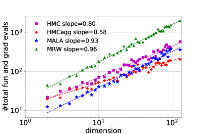
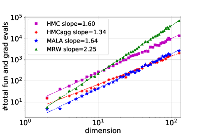
(a) $\kappa=4$	(b) $\kappa=d^{\frac{2}{3}}$

Figure 2: Average number of total function and gradient evaluations as a function of dimension for four random walks on multivariate Gaussian density (24) where the covariance has a condition number $\kappa$ that is (a) constant $4$ and (b) scales with dimension $d$. With suggested step-size and leapfrog steps in Corollary 2, the number of total function and gradient evaluations of HMC has a smaller dimension dependency than that of MALA or MRW. Since the target distributon is Gaussian and the Hessian-Lipschitz constant $L_{\text{H}}$ is zero, larger step-size and larger number of leapfrog steps can be chosen according to Appendix D.1.1. The plots does show that HMCagg with larger step-size and larger number of leapfrog steps uses smaller number of total function and gradient evaluations to achieve the same quantile mixing.

(b) Dimension dependency for $\kappa=d^{2/3}$:

Next, we consider target distributions such that their condition number varies with $d$ as $\kappa=d^{2/3}$, where $d$ is varied from $2$ to $128$. To ensure such a scaling for $\kappa$, we choose the Hessian $\Sigma$ for the multivariate Gaussian distribution to be diagonal and set the square roots of its eigenvalues linearly spaced between $1.0$ to $d^{1/3}$. Figure 2(b) shows the dependency of the number of total function and gradient evaluations as a function of dimension $d$ for the four random walks on the log-log scale. The least squares fits yield the slopes as $1.60(\pm 0.09)$, $1.34(\pm 0.17)$, $1.64(\pm 0.11)$ and $2.25(\pm 0.08)$ for HMC, HMCagg, MALA and MRW, respectively, where standard errors of the regression coefficient are reported in the parentheses. Recall that the theoretical guarantees for HMC (Table 5), HMCagg (Table 6), MALA and MRW (Table 2) yield that these exponent should be close to 1.58, 1.46, 1.67 and 2.33 respectively. Once again, we observe a good agreement of the numerical results with that of our theoretical results.

Remark:

We would like to caution that the aggressive parameter choices for HMCagg are well-informed only when the Hessian-Lipschitz constant $L_{\text{H}}$ is small—which indeed is the case for the Gaussian target distributions considered above. When general log-concave distributions are considered, one may use the more general choices recommended in Corollary 14. See Appendix D for an in-depth discussion on different scenarios and the optimal parameter choices derived from our theory.

5 Proofs

This section is devoted primarily to the proof of Theorem 1. In order to do so, we begin with the mixing time bound based on the conductance profile from Lemma 3. We then seek to apply Lemma 4 in order derive a bound on the conductance profile itself. However, in order to do so, we need to derive bound on the overlap between the proposal distributions of HMC at two nearby points and show that the Metropolis-Hastings step only modifies the proposal distribution by a relatively small amount. This control is provided by Lemma 6, stated in Section 5.1. We use it to prove Theorem 1 in Section 5.2. Finally, Section 5.3 is devoted to the proof of Lemma 6. We provide a sketch-diagram for how various main results of the paper interact with each other in Figure 1.

5.1 Overlap bounds for HMC

In this subsection, we derive two important bounds for the Metropolized HMC chain: (1) first, we quantify the overlap between proposal distributions of the chain for nearby points, and, (2) second, we show that the distortion in the proposal distribution introduced by the Metropolis-Hastings accept-reject step can be controlled if an appropriate step-size is chosen. Putting the two pieces together enables us to invoke Lemma 4 to prove Theorem 1.

In order to do so, we begin with some notation. Let $\mathcal{T}$ denote the transition operator of the HMC chain with leapfrog integrator taking step-size $\eta$ and number of leapfrog updates $K$. Let $\mathcal{P}_{x}$ denote the proposal distribution at $x\in\mathcal{X}$ for the chain before the accept-reject step and the lazy step. Let $\mathcal{T}^{\text{before-lazy}}_{x}$ denote the corresponding transition distribution after the proposal and the accept-reject step, before the lazy step. By definition, we have

$$\mathcal{T}_{x}(A)=\zeta\mathbf{\delta}_{x}(A)+(1-\zeta)\mathcal{T}^{\text{before-lazy}}_{x}(A)\qquad\mbox{for any measurable set $A\in\mathcal{B}(\mathcal{X})$.}$$ (25)

Our proofs make use of the Euclidean ball $\mathcal{R}_{s}$ defined in equation (29). At a high level, the HMC chain has bounded gradient inside the ball $\mathcal{R}_{s}$ for a suitable choice of $s$, and the gradient of the log-density gets too large outside such a ball making the chain unstable in that region. However, since the target distribution has low mass in that region, the chain’s visit to the region outside the ball is a rare event and thus we can focus on the chain’s behavior inside the ball to analyze its mixing time.

In the next lemma, we state the overlap bounds for the transition distributions of the HMC chain. For a fixed univeral constant $c$, we require

$$K^{2}\eta^{2} \leq\frac{1}{4\max\left\{d^{\frac{1}{2}}L,d^{\frac{2}{3}}L_{\text{H}}^{\frac{2}{3}}\right\}},\qquad\mbox{and}$$ (26a)

$$\eta^{2} \leq\frac{1}{cL}\min\left\{\frac{1}{K^{2}},\frac{1}{Kd^{\frac{1}{2}}},\frac{1}{K^{\frac{2}{3}}d^{\frac{1}{3}}\left(\frac{M^{2}}{L}\right)^{\frac{1}{3}}},\frac{1}{K\frac{M}{L^{\frac{1}{2}}}},\frac{1}{K^{\frac{2}{3}}d}\frac{L}{L_{\text{H}}^{\frac{2}{3}}},\frac{1}{K^{\frac{4}{3}}\frac{M}{L^{\frac{1}{2}}}}\left(\frac{L}{L_{\text{H}}^{\frac{2}{3}}}\right)^{\frac{1}{2}}\right\}.$$ (26b)

Lemma 6

Consider a $(L,L_{\text{H}},s,\psi_{\mathfrak{a}},M)$-regular target distribution (cf. Assumption (A)) with $\Omega$ the convex measurable set satisfying (10e). Then with the parameters $\left(K,\eta\right)$ satisfying $K\eta\leq\frac{1}{4L}$ and condition (26a), the HMC-$\left(K,\eta\right)$ chain satisfies

$$\sup_{\left\|q_{0}-{\tilde{q}}_{0}\right\|_{2}\leq\frac{K\eta}{4}}d_{\text{\tiny{TV}}}\left(\mathcal{P}_{q_{0}},\mathcal{P}_{{\tilde{q}}_{0}}\right)\leq\frac{1}{2}.$$ (27a)

If, in addition, condition (26b) holds, then we have

$$\sup_{x\in\Omega}d_{\text{\tiny{TV}}}\left(\mathcal{P}_{x},\mathcal{T}^{\text{before-lazy}}_{x}\right)\leq\frac{1}{8}.$$ (27b)

See Appendix 5.3 for the proof.

Lemma 6 is crucial to the analysis of HMC as it enables us to apply the conductance profile based bounds discussed in Section 3.3. It reveals two important properties of the Metropolized HMC. First, from equation (27a), we see that proposal distributions of HMC at two different points are close if the two points are close. This is proved by controlling the KL-divergence of the two proposal distributions of HMC via change of variable formula. Second, equation (27b) shows that the accept-reject step of HMC is well behaved inside $\Omega$ provided the gradient is bounded by $M$.

5.2 Proof of Theorem 1

We are now equipped to prove our main theorem. In order to prove Theorem 1, we begin by using Lemma 4 and Lemma 6 to derive an explicit bound for on the HMC conductance profile. Given the assumptions of Theorem 1, conditions (26a) and (26b) hold, enabling us to invoke Lemma 6 in the proof.

Define the function $\Psi_{\Omega}:[0,1]\mapsto{}_{+}$ as

$$\Psi_{\Omega}(v) =\begin{cases}\displaystyle\frac{1}{32}\cdot\min\left\{1,\frac{K\eta}{64\psi_{\mathfrak{a}}}\log^{\mathfrak{a}}\left(\frac{1}{v}\right)\right\}&\mbox{if $v\in\left[0,\frac{1-s}{2}\right]$.}\\[8.53581pt] \displaystyle\frac{K\eta}{2048\psi_{\mathfrak{a}}},&\mbox{if $v\in\left(\frac{1-s}{2},1\right]$.}\end{cases}$$ (28)

This function acts as a lower bound on the truncated conductance profile. Define the Euclidean ball

$$\mathcal{R}_{s}=\mathbb{B}\left(x^{\star},r(s)\sqrt{\frac{d}{m}}\right),$$ (29)

and consider a pair $(x,y)\in\mathcal{R}_{s}$ such that $\left\|x-y\right\|_{2}\leq\frac{1}{4}K\eta$. Invoking the decomposition (25) and applying triangle inequality for $\zeta$-lazy HMC, we have

$$d_{\text{\tiny{TV}}}\left(\mathcal{T}_{x},\mathcal{T}_{y}\right) \leq\zeta+\left(1-\zeta\right)d_{\text{\tiny{TV}}}\left(\mathcal{T}^{\text{before-lazy}}_{x},\mathcal{T}^{\text{before-lazy}}_{y}\right)$$

$$\leq\zeta+\left(1-\zeta\right)\left(d_{\text{\tiny{TV}}}\left(\mathcal{T}^{\text{before-lazy}}_{x},\mathcal{P}_{y}\right)+d_{\text{\tiny{TV}}}\left(\mathcal{P}_{x},\mathcal{P}_{y}\right)+d_{\text{\tiny{TV}}}\left(\mathcal{P}_{x},\mathcal{T}^{\text{before-lazy}}_{y}\right)\right)$$

$$\stackrel{{\scriptstyle(i)}}{{\leq}}\zeta+\left(1-\zeta\right)\left(\frac{1}{4}+\frac{1}{2}+\frac{1}{4}\right)$$

$$=1-\frac{1-\zeta}{4},$$

where step (i) follows from the bounds (27a) and (27b) from Lemma 6. For $\zeta=\frac{1}{2}$, substituting $\omega=\frac{1}{8}$, $\Delta=\frac{1}{4}K\eta$ and the convex set $\Omega=\mathcal{R}_{s}$ into Lemma 4, we obtain that

$$\Phi_{\Omega}(v)\geq\frac{1}{32}\cdot\min\left\{1,\frac{K\eta}{64\psi_{\mathfrak{a}}}\log^{\mathfrak{a}}\left(1+\frac{1}{v}\right)\right\},\quad\text{for }v\in\left[0,\frac{1-s}{2}\right].$$

Here $\mathfrak{a}$ equals to $\frac{1}{2}$ or $0$, depending on the assumption (10d). By the definition of the truncated conductance profile (15), we have that $\tilde{\Phi}_{\Omega}(v)\geq\frac{K\eta}{2048\psi_{\mathfrak{a}}}$ for $v\in\left[\frac{1-s}{2},1\right]$. As a consequence, $\Psi_{\Omega}$ is effectively a lower bound on the truncated conductance profile. Note that the assumption (A) ensures the existence of $\Omega$ such that $\Pi^{*}(\Omega)\geq 1-s$ for $s=\frac{\epsilon^{2}}{3\beta^{2}}$. Putting the pieces together and applying Lemma 3 with the convex set $\Omega$ concludes the proof of the theorem.

5.3 Proof of Lemma 6

In this subsection, we prove the two main claims (27a) and (27b) in Lemma 6. Before going into the claims, we first provide several convenient properties about the HMC proposal.

5.3.1 Properties of the HMC proposal

Recall the Hamiltonian Monte Carlo (HMC) with leapfrog integrator (8c). Using an induction argument, we find that the final states in one iteration of $K$ steps of the HMC chain, denoted by $q_{K}$ and $p_{K}$ satisfy

$$p_{K} =p_{0}-\frac{\eta}{2}{\nabla f}(q_{0})-\sum_{j=1}^{K-1}{\nabla f}(q_{j})-\frac{\eta}{2}{\nabla f}(q_{K}),$$ (30a)

$$\quad\text{and}\quad q_{K} =q_{0}+K\eta p_{0}-\frac{K\eta^{2}}{2}{\nabla f}(q_{0})-\eta^{2}\sum_{j=1}^{K-1}\left(K-j\right){\nabla f}(q_{j}).$$ (30b)

It is easy to see that for $$k\in\left[K\right] q_{k} q_{0} p_{0} F$$, can be seen as a function of the initial state and . We denote this function as the forward mapping ,

$$q_{k}=:F_{k}(p_{0},q_{0})\quad\text{and}\quad q_{K}=:F_{K}(p_{0},q_{0})=:F\left(p_{0},q_{0}\right)$$ (30c)

where we introduced the simpler notation $$F:\,=F_{K} F_{k} F {\nabla f} K \eta$$ for the final iterate. The forward mappings and are deterministic functions that only depends on the gradient , the number of leapfrog updates and the step size .

Denote $\mathbf{J}_{x}F$ as the Jacobian matrix of the forward mapping $F$ with respect to the first variable. By definition, it satisfies

$$\left[\mathbf{J}_{x}F(x,q_{0})\right]_{ij}=\frac{\partial}{\partial x_{j}}\left[F(x,q_{0})\right]_{i},\quad\text{for all}\quad i,j\in\left[d\right].$$ (30d)

Similarly, denote $\mathbf{J}_{y}F$ as the Jacobian matrix of the forward mapping $F$ with respect to the second variable. The following lemma characterizes the eigenvalues of the Jacobian $\mathbf{J}_{x}F$.

Lemma 7

Suppose the log density $f$ is $L$-smooth. For the number of leapfrog steps and step-size satisfying $K^{2}\eta^{2}\leq\frac{1}{4L}$, we have

$$\left|\!\left|\!\left|K\eta\mathbb{I}_{d}-\mathbf{J}_{x}F(x,y)\right|\!\right|\!\right|_{{2}}\leq\frac{1}{8}K\eta,\quad\text{for all}\quad x,y\in\mathcal{X}\text{ and }i\in\left[d\right].$$

Also all eigenvalues of $\mathbf{J}_{x}F(x,y)$ have absolute value greater or equal to $\frac{7}{8}K\eta$.

See Appendix A.3.1 for the proof.

Since the Jacobian is invertible for $K^{2}\eta^{2}\leq\frac{1}{4L}$, we can define the inverse function of $F$ with respect to the first variable as the backward mapping $G$. We have

$$F\left(G(x,y),y\right)=x,\quad\text{for all}\quad x,y\in\mathcal{X}.$$ (31)

Moreover as a direct consequence of Lemma 7, we obtain that the magnitude of the eigenvalues of the Jacobian matrix $\mathbf{J}_{x}G(x,y)$ lies in the interval $\left[\frac{8}{9K\eta},\frac{8}{7K\eta}\right]$. In the next lemma, we state another set of bounds on different Jacobian matrices:

Lemma 8

Suppose the log density $f$ is $L$-smooth. For the number of leapfrog steps and step-size satisfying $K^{2}\eta^{2}\leq\frac{1}{4L}$, we have

$$\left|\!\left|\!\left|\mathbf{J}_{y}G(x,y)\right|\!\right|\!\right|_{{2}} \leq\frac{4}{3K\eta},\quad\text{for all}\quad x,y\in\mathcal{X},\quad\text{and}\quad$$ (32a)

$$\left|\!\left|\!\left|\frac{\partial F_{k}(G(x,y),y)}{\partial y}\right|\!\right|\!\right|_{{2}} \leq 3,\quad\quad\text{for all}\quad k\in\left[K\right].$$ (32b)

See Appendix A.3.2 for the proof.

Next, we would like to obtain a bound on the quantity $\frac{\partial\log\det\mathbf{J}_{x}G(x,q_{0})}{\partial y}$. Applying the chain rule, we find that

$$\frac{\partial\log\det\mathbf{J}_{x}G(x,q_{0})}{\partial y}=\begin{bmatrix}\operatorname{\text{trace}}\left([\mathbf{J}_{x}G(x,q_{0})]^{-1}\mathbf{J}_{xy_{1}}G(x,q_{0})\right)\\ \vdots\\ \operatorname{\text{trace}}\left([\mathbf{J}_{x}G(x,q_{0})]^{-1}\mathbf{J}_{xy_{d}}G(x,q_{0})\right)\end{bmatrix}.$$ (33)

Here $\mathbf{J}_{xy}G(x,q_{0})$ is a third order tensor and we use $\mathbf{J}_{xy_{l}}G(x,q_{0})$ to denote the matrix corresponding to the $l$-th slice of the tensor which satisfies

$$\left[\mathbf{J}_{xy_{l}}G(x,q_{0})\right]_{ij}=\frac{\partial\partial}{\partial x_{j}y_{l}}\left[F(x,q_{0})\right]_{i},\ \quad\text{for all}\quad i,j,l\in\left[d\right].$$

Lemma 9

Suppose the log density $f$ is $L$-smooth and $L_{\text{H}}$-Hessian Lipschitz. For the number of leapfrog steps and step-size satisfying $K^{2}\eta^{2}\leq\frac{1}{4L}$, we have

$$\left\|\frac{\partial\log\det\mathbf{J}_{x}G(x,q_{0})}{\partial y}\right\|_{2}=\left\|\begin{bmatrix}\operatorname{\text{trace}}\left([\mathbf{J}_{x}G(x,q_{0})]^{-1}\mathbf{J}_{xy_{1}}G(x,q_{0})\right)\\ \vdots\\ \operatorname{\text{trace}}\left([\mathbf{J}_{x}G(x,q_{0})]^{-1}\mathbf{J}_{xy_{d}}G(x,q_{0})\right)\end{bmatrix}\right\|_{2}\leq 2dK^{2}\eta^{2}L_{\text{H}}.$$

See Appendix A.3.3 for the proof.

As a direct consequence of the equation (30b) at $k$-th step of leapfrog updates, we obtain the following two bounds for the difference between successive $F_{k}$ terms that come in handy later in our proofs.

Lemma 10

Suppose that the log density $f$ is $L$-smooth. For the number of leapfrog steps and step-size satisfying $K^{2}\eta^{2}\leq\frac{1}{4L}$, we have

$$\left\|F_{k}(p_{0},q_{0})-q_{0}\right\|_{2} \leq 2k\eta\left\|p_{0}\right\|_{2}+2k^{2}\eta^{2}\left\|{\nabla f}(q_{0})\right\|_{2}\ \ \text{for }k\in\left[K\right],\ \text{and}$$ (34a)

$$\left\|F_{k+1}(p_{0},q_{0})-F_{k}(p_{0},q_{0})\right\|_{2} \leq 2\eta\left\|p_{0}\right\|_{2}+2(k+1)\eta^{2}\left\|{\nabla f}(q_{0})\right\|_{2}\ \text{for }k\in\left[K-1\right].$$ (34b)

See Appendix A.3.4 for the proof.

We now turn to the proof the two claims in Lemma 6. Note that the claim (27a) states that the proposal distributions at two close points are close; the claim (27b) states that the proposal distribution and the transition distribution are close.

5.3.2 Proof of claim (27a) in Lemma 6

In order to bound the distance between proposal distributions of nearby points, we prove the following stronger claim: For a $L$-smooth $L_{\text{H}}$-Hessian-Lipschitz target distribution, the proposal distribution of the HMC algorithm with step size $\eta$ and leapfrog steps $K$ such that $K\eta\leq\frac{1}{4L}$ satisfies

$$d_{\text{\tiny{TV}}}\left(\mathcal{P}_{q_{0}},\mathcal{P}_{{\tilde{q}}_{0}}\right)\leq\left(\frac{2\left\|q_{0}-{\tilde{q}}_{0}\right\|_{2}^{2}}{K^{2}\eta^{2}}+3\sqrt{d}K\eta L\left\|q_{0}-{\tilde{q}}_{0}\right\|_{2}+4dK^{2}\eta^{2}L_{\text{H}}\left\|q_{0}-{\tilde{q}}_{0}\right\|_{2}\right)^{1/2},$$ (35)

for all $q_{0},{\tilde{q}}_{0}\in{}^{d}$. Then for any two points $q_{0},{\tilde{q}}_{0}$ such that $\left\|q_{0}-{\tilde{q}}_{0}\right\|_{2}\leq\frac{1}{4}K\eta$, under the condition (26a), i.e., $K^{2}\eta^{2}\leq\frac{1}{4\max\left\{d^{\frac{1}{2}}L,d^{\frac{2}{3}}L_{\text{H}}^{\frac{2}{3}}\right\}}$, we have

$$d_{\text{\tiny{TV}}}\left(\mathcal{P}_{q_{0}},\mathcal{P}_{{\tilde{q}}_{0}}\right)\leq\left(\frac{1}{8}+\frac{3}{64}+\frac{1}{64}\right)^{1/2}\leq\frac{1}{2},$$

and the claim (27a) follows.

The proof of claim (35) involves the following steps: (1) we make use of the update rules (30b) and change of variable formula to obtain an expression for the density of $q_{n}$ in terms of $q_{0}$, (2) then we use Pinsker’s inequality and derive expressions for the KL-divergence between the two proposal distributions, and (3) finally, we upper bound the KL-divergence between the two distributions using different properties of the forward mapping $F$ from Appendix 5.3.1.

According to the update rule (30b), the proposals from two initial points $q_{0}$ and ${\tilde{q}}_{0}$ satisfy respectively

$$q_{K}=F(p_{0},q_{0}),\quad\text{ and }\quad{\tilde{q}}_{K}=F({\tilde{p}}_{0},{\tilde{q}}_{0}),$$

where $p_{0}$ and ${\tilde{p}}_{0}$ are independent random variable from Gaussian distribution $\mathcal{N}(0,\mathbb{I}_{d})$.

Denote $\rho_{q_{0}}$ as the density function of the proposal distribution $\mathcal{P}_{q_{0}}$. For two different initial points $q_{0}$ and ${\tilde{q}}_{0}$, the goal is to bound the total variation distance between the two proposal distribution, which is by definition

$$d_{\text{\tiny{TV}}}\left(\mathcal{P}_{q_{0}},\mathcal{P}_{{\tilde{q}}_{0}}\right)=\frac{1}{2}\int_{x\in\mathcal{X}}\left|\rho_{q_{0}}(x)-\rho_{{\tilde{q}}_{0}}(x)\right|dx.$$ (36)

Given $q_{0}$ fixed, the random variable $q_{K}$ can be seen as a transformation of the Gaussian random variable $p_{0}$ through the function $F(\cdot,q_{0})$. When $F$ is invertible, we can use the change of variable formula to obtain an explicit expression of the density $\rho_{q_{0}}$:

$$\rho_{q_{0}}(x)=\varphi\left(G(x,q_{0})\right)\det\left(\mathbf{J}_{x}G(x,q_{0})\right),$$ (37)

where $\varphi$ is the density of the standard Gaussian distribution $\mathcal{N}(0,\mathbb{I}_{d})$. Note that even though explicit, directly bounding the total variation distance (36) using the complicated density expression (37) is difficult. We first use Pinsker’s inequality (Cover and Thomas, 1991) to give an upper bound of the total variance distance in terms of KL-divergence

$$d_{\text{\tiny{TV}}}\left(\mathcal{P}_{q_{0}},\mathcal{P}_{{\tilde{q}}_{0}}\right)\leq\sqrt{2\text{KL}(\mathcal{P}_{q_{0}}\;\|\;\mathcal{P}_{{\tilde{q}}_{0}})},$$ (38)

and then upper bound the KL-divergence. Plugging the density (37) into the KL-divergence formula, we obtain that

$$\text{KL}(\mathcal{P}_{q_{0}}\;\|\;\mathcal{P}_{{\tilde{q}}_{0}}) =\int_{{}^{d}}\rho_{q_{0}}(x)\log\left(\frac{\rho_{q_{0}}(x)}{\rho_{{\tilde{q}}_{0}}(x)}\right)dx$$

$$=\int_{{}^{d}}\rho_{q_{0}}(x)\left[\log\left(\frac{\varphi\left(G(x,q_{0})\right)}{\varphi\left(G(x,{\tilde{q}}_{0})\right)}\right)+\log\det\mathbf{J}_{x}G(x,q_{0})-\log\det\mathbf{J}_{x}G(x,{\tilde{q}}_{0})\right]dx$$

$$=\underbrace{\int_{{}^{d}}\rho_{q_{0}}(x)\left[\frac{1}{2}\left(-\left\|G(x,q_{0})\right\|_{2}^{2}+\left\|G(x,{\tilde{q}}_{0})\right\|_{2}^{2}\right)\right]dx}_{T_{1}}$$

$$\quad\quad\quad\quad+\underbrace{\int_{{}^{d}}\rho_{q_{0}}(x)\left[\log\det\mathbf{J}_{x}G(x,q_{0})-\log\det\mathbf{J}_{x}G(x,{\tilde{q}}_{0})\right]dx}_{T_{2}}$$ (39)

We claim the following bounds on the terms $T_{1}$ and $T_{2}$:

$$\left|T_{1}\right| \leq\frac{8}{9}\frac{\left\|q_{0}-{\tilde{q}}_{0}\right\|_{2}^{2}}{K^{2}\eta^{2}}+\frac{3}{2}\sqrt{d}K\eta L\left\|q_{0}-{\tilde{q}}_{0}\right\|_{2},\quad\text{and}$$ (40a)

$$\left|T_{2}\right| \leq 2dK^{2}\eta^{2}L_{\text{H}}\left\|q_{0}-{\tilde{q}}_{0}\right\|_{2},$$ (40b)

where the bound on $T_{2}$ follows readily from Lemma 9:

$$\left|T_{2}\right| =\left|\int\rho_{q_{0}}(x)\left[\log\det\mathbf{J}_{x}G(x,q_{0})-\log\det\mathbf{J}_{x}G(x,{\tilde{q}}_{0})\right]dx\right|$$

$$\leq\left\|\frac{\partial\log\det\mathbf{J}_{x}G(x,q_{0})}{\partial y}\right\|_{2}\left\|q_{0}-{\tilde{q}}_{0}\right\|_{2}$$

$$\leq 2dK^{2}\eta^{2}L_{\text{H}}\left\|q_{0}-{\tilde{q}}_{0}\right\|_{2}.$$ (41)

Putting together the inequalities (38), (5.3.2), (40a) and (40b) yields the claim (35).

It remains to prove the bound (40a) on $T_{1}$.

Proof of claim (40a):

For the term $T_{1}$, we observe that

$$\frac{1}{2}\left(\left\|G(x,{\tilde{q}}_{0})\right\|_{2}^{2}-\left\|G(x,q_{0})\right\|_{2}^{2}\right)=\frac{1}{2}\left\|G(x,q_{0})-G(x,{\tilde{q}}_{0})\right\|_{2}^{2}-\left(G(x,q_{0})-G(x,{\tilde{q}}_{0})\right)^{\top}G(x,q_{0}).$$

The first term on the RHS can be bounded via the Jacobian of $G$ with respect to the second variable. Applying the bound (32a) from Lemma 8, we find that

$$\left\|G(x,q_{0})-G(x,{\tilde{q}}_{0})\right\|_{2}\leq\left|\!\left|\!\left|\mathbf{J}_{y}G(x,y)\right|\!\right|\!\right|_{{2}}\left\|q_{0}-{\tilde{q}}_{0})\right\|_{2}\leq\frac{4}{3K\eta}\left\|q_{0}-{\tilde{q}}_{0})\right\|_{2}.$$ (42)

For the second part, we claim that there exists a deterministic function $C$ of $q_{0}$ and ${\tilde{q}}_{0}$ and independent of $x$, such that

$$\left\|G(x,q_{0})-G(x,{\tilde{q}}_{0})-C(q_{0},{\tilde{q}}_{0})\right\|_{2}\leq\frac{3}{2}K\eta L\left\|q_{0}-{\tilde{q}}_{0}\right\|_{2}.$$ (43)

Assuming the claim (43) as given at the moment, we can further decompose the second part of $T_{1}$ into two parts:

$$\left(G(x,q_{0})-G(x,{\tilde{q}}_{0})\right)^{\top}G(x,q_{0})=\left(G(x,q_{0})-G(x,{\tilde{q}}_{0})-C(q_{0},{\tilde{q}}_{0})\right)^{\top}G(x,q_{0})+C(q_{0},{\tilde{q}}_{0})^{\top}G(x,q_{0})$$ (44)

Applying change of variables along with equation (37), we find that

$$\int\rho_{q_{0}}(x)G(x,q_{0})dx=\int\varphi(x)xdx=0.$$

Furthermore, we also have

$$\int_{x\in\mathcal{X}}\rho_{q_{0}}(x)\left\|G(x,q_{0})\right\|_{2}dx =\int_{x\in\mathcal{X}}\varphi(x)\left\|x\right\|_{2}dx$$

$$\stackrel{{\scriptstyle(i)}}{{\leq}}\left[\left(\int_{x\in\mathcal{X}}\varphi(x)\left\|x\right\|_{2}^{2}dx\right){\left(\int_{x\in\mathcal{X}}\varphi(x)dx\right)}\right]^{1/2}=\sqrt{d},$$

where step (i) follows from Cauchy-Schwarz’s inequality. Combining the inequalities (42), (43) and (44) together, we obtain the following bound on term $T_{1}$:

$$\left|T_{1}\right| =\left|\int\rho_{q_{0}}(x)\left[-\frac{1}{2}\left\|G(x,q_{0})\right\|_{2}^{2}+\frac{1}{2}\left\|G(x,{\tilde{q}}_{0})\right\|_{2}^{2}\right]dx\right|$$

$$\leq\frac{1}{2}\left|\int\rho_{q_{0}}(x)\left\|G(x,q_{0})-G(x,{\tilde{q}}_{0})\right\|_{2}^{2}dx\right|$$

$$\qquad\qquad\qquad+\left|\int\rho_{q_{0}}(x)\left\|G(x,q_{0})-G(x,{\tilde{q}}_{0})-C(q_{0},{\tilde{q}}_{0})\right\|_{2}\left\|G(x,q_{0})\right\|_{2}dx\right|$$

$$\leq\frac{8}{9}\frac{\left\|q_{0}-{\tilde{q}}_{0}\right\|_{2}^{2}}{K^{2}\eta^{2}}+\frac{3}{2}\sqrt{d}K\eta\left\|q_{0}-{\tilde{q}}_{0}\right\|_{2},$$ (45)

which yields the claimed bound on $T_{1}$.

We now prove our earlier claim (43).

Proof of claim (43):

For any pair of states $q_{0}$ and ${\tilde{q}}_{0}$, invoking the definition (31) of the map $G(x,\cdot)$, we obtain the following implicit equations:

$$x =q_{0}+K\eta G(x,q_{0})-K\frac{\eta^{2}}{2}{\nabla f}(q_{0})-\eta^{2}\sum_{j=1}^{K-1}(K-j){\nabla f}(F_{j}(G(x,q_{0}),q_{0})),\quad\text{and}$$

$$x ={\tilde{q}}_{0}+K\eta G(x,{\tilde{q}}_{0})-K\frac{\eta^{2}}{2}{\nabla f}({\tilde{q}}_{0})-\eta^{2}\sum_{j=1}^{K-1}(K-j){\nabla f}(F_{j}(G(x,{\tilde{q}}_{0}),{\tilde{q}}_{0})).$$

Taking the difference between the two equations above, we obtain

$$G(x,q_{0})-G(x,{\tilde{q}}_{0}) -\frac{q_{0}-{\tilde{q}}_{0}}{K\eta}-\frac{\eta}{2}\left({\nabla f}(q_{0})-{\nabla f}({\tilde{q}}_{0})\right)$$

$$=\frac{\eta^{2}}{K\eta}\sum_{k=1}^{K-1}(K-j)\left({\nabla f}(F_{k}(G(x,q_{0}),q_{0}))-{\nabla f}(F_{k}(G(x,{\tilde{q}}_{0}),{\tilde{q}}_{0}))\right).$$

Applying $L$-smoothness of $f$ along with the bound (32b) from Lemma 8, we find that

$$\left\|{\nabla f}(F_{k}(G(x,q_{0}),q_{0}))-{\nabla f}(F_{k}(G(x,{\tilde{q}}_{0}),{\tilde{q}}_{0}))\right\|_{2} \leq L\left|\!\left|\!\left|\frac{\partial F_{k}(G(x,y),y)}{\partial y}\right|\!\right|\!\right|_{{2}}\left\|q_{0}-{\tilde{q}}_{0}\right\|_{2}$$

$$\leq 3L\left\|q_{0}-{\tilde{q}}_{0}\right\|_{2}.$$

Putting the pieces together, we find that

$$\left\|G(x,q_{0})-G(x,{\tilde{q}}_{0})-\frac{q_{0}-{\tilde{q}}_{0}}{K\eta}-\frac{1}{2}\left({\nabla f}(q_{0})-{\nabla f}({\tilde{q}}_{0})\right)\right\|_{2}\leq\frac{3K\eta L}{2}\left\|q_{0}-{\tilde{q}}_{0}\right\|_{2},$$

which yields the claim (43).

5.3.3 Proof of claim (27b) in Lemma 6

We now bound the distance between the one-step proposal distribution $\mathcal{P}_{x}$ at point $x$ and the one-step transition distribution $\mathcal{T}^{\text{before-lazy}}_{x}$ at $x$ obtained after performing the accept-reject step (and no lazy step). Using equation (30a), we define the forward mapping $E$ for the variable $p_{K}$ as follows

$$p_{K}=E(p_{0},q_{0}):\,=p_{0}-\frac{\eta}{2}{\nabla f}(q_{0})-\eta\sum_{j=1}^{K-1}{\nabla f}(q_{j})-\frac{\eta}{2}{\nabla f}(q_{K}).$$

Consequently, the probability of staying at $x$ is given by

$$\mathcal{T}^{\text{before-lazy}}_{x}(\left\{x\right\})=1-\int_{\mathcal{X}}\min\left\{1,\frac{\exp(-\mathcal{H}(E(z,x),F(z,x)))}{\exp(-\mathcal{H}(z,x))}\right\}\varphi_{x}(z)dz,$$

where the Hamiltonian $\mathcal{H}(q,p)=f(q)+\frac{1}{2}\left\|p\right\|_{2}^{2}$ was defined in equation (7). As a result, the TV-distance between the proposal and transition distribution is given by

$$d_{\text{\tiny{TV}}}\left(\mathcal{P}_{x},\mathcal{T}^{\text{before-lazy}}_{x}\right) =1-\int_{\mathcal{X}}\min\left\{1,\frac{\exp(-\mathcal{H}(E(z,x),F(z,x)))}{\exp(-\mathcal{H}(z,x))}\right\}\varphi_{x}(z)dz$$

$$=1-{\mathbb{E}}_{z\sim\mathcal{N}(0,\mathbb{I}_{d})}\left[\min\left\{1,\frac{\exp(-\mathcal{H}(E(z,x),F(z,x)))}{\exp(-\mathcal{H}(z,x))}\right\}\right].$$ (46)

An application of Markov’s inequality yields that

$${\mathbb{E}}_{z\sim\mathcal{N}(0,\mathbb{I}_{d})}\left[\min\left\{1,\frac{\exp(-\mathcal{H}(E(z,x),F(z,x)))}{\exp(-\mathcal{H}(z,x))}\right\}\right]$$

$$\qquad\geq\alpha{\mathbb{P}}_{z\sim\mathcal{N}(0,\mathbb{I}_{d})}\left[\frac{\exp(-\mathcal{H}(E(z,x),F(z,x)))}{\exp(-\mathcal{H}(z,x))}\geq\alpha\right],$$ (47)

for any $\alpha\in(0,1]$. Thus, to bound the distance $d_{\text{\tiny{TV}}}\left(\mathcal{P}_{x},\mathcal{T}^{\text{before-lazy}}_{x}\right)$, it suffices to derive a high probability lower bound on the ratio ${\exp(-\mathcal{H}(E(z,x),F(z,x)))}/{\exp(-\mathcal{H}(z,x))}$ when $z\sim\mathcal{N}(0,\mathbb{I}_{d})$.

We now derive a lower bound on the following quantity:

$$\exp\left(-f(F(p_{0},q_{0}))+f(q_{0})-\frac{1}{2}\left\|E(p_{0},q_{0})\right\|_{2}^{2}+\frac{1}{2}\left\|p_{0}\right\|_{2}^{2}\right),\quad\mbox{when $p_{0}\sim\mathcal{N}(0,\mathbb{I}_{d})$.}$$

We derive the bounds on the two terms $-f(F(p_{0},q_{0}))+f(q_{0})$ and $\left\|E(p_{0},q_{0})\right\|_{2}^{2}$ separately.

Observe that

$$f(F(p_{0},q_{0}))-f(q_{0})=\sum_{j=0}^{K-1}\left[f(F_{j+1}(p_{0},q_{0}))-f(F_{j}(p_{0},q_{0}))\right].$$

The intuition is that it is better to apply Taylor expansion on closer points. Applying the third order Taylor expansion and using the smoothness assumptions (10a) and (10c) for the function $f$, we obtain

$$f(x)-f(y)\leq\frac{(x-y)^{\top}}{2}\left({\nabla f}(x)+{\nabla f}(y)\right)+L_{\text{H}}\left\|x-y\right\|_{2}^{3}.$$

For the indices $j\in\left\{0,\ldots,K-1\right\}$, using $F_{j}$ as the shorthand for $F_{j}(p_{0},q_{0})$, we find that

$$f(F_{j+1})-f(F_{j}) \leq\frac{(F_{j+1}-F_{j})^{\top}}{2}\left({\nabla f}(F_{j+1})+{\nabla f}(F_{j})\right)+L_{\text{H}}\left\|F_{j+1}-F_{j}\right\|_{2}^{3}$$

$$=\frac{1}{2}\eta p_{0}^{\top}\left({\nabla f}(F_{j+1})+{\nabla f}(F_{j})\right)$$

$$\quad-\frac{\eta^{2}}{2}\bigg{[}{\frac{1}{2}{\nabla f}(p_{0})+\sum_{k=1}^{j}{\nabla f}(F_{k})}\bigg{]}^{\top}\left({\nabla f}(F_{j+1})+{\nabla f}(F_{j})\right)+L_{\text{H}}\left\|F_{j+1}-F_{j}\right\|_{2}^{3},$$ (48)

where the last equality follows by definition (30c) of the operator $F_{j}$.

Now to bound the term $E(p_{0},q_{0})$, we observe that

$$\frac{\left\|E(p_{0},q_{0})\right\|_{2}^{2}}{2} =\frac{\left\|p_{0}-\frac{\eta}{2}{\nabla f}(q_{0})-\eta\sum_{j=1}^{K-1}{\nabla f}(F_{j})-\frac{\eta}{2}{\nabla f}(F_{K})\right\|_{2}^{2}}{2}$$

$$=\frac{\left\|p_{0}\right\|_{2}^{2}}{2}-\eta p_{0}^{\top}\bigg{(}{\frac{1}{2}{\nabla f}(q_{0})+\sum_{j=1}^{K-1}{\nabla f}(F_{j})+\frac{1}{2}{\nabla f}(F_{K})}\bigg{)}$$

$$\qquad\qquad\qquad+\frac{\eta^{2}}{2}\big{\|}{\frac{1}{2}{\nabla f}(q_{0})+\sum_{j=1}^{K-1}{\nabla f}(F_{j})+\frac{1}{2}{\nabla f}(F_{K})}\big{\|}_{2}^{2}.$$ (49)

Putting the equations (5.3.3) and (49) together leads to cancellation of many gradient terms and we obtain

$$-f(F(p_{0},q_{0}))+f(q_{0})-\frac{1}{2}\left\|E(p_{0},q_{0})\right\|_{2}^{2}+\frac{1}{2}\left\|p_{0}\right\|_{2}^{2}$$

$$\quad\geq\frac{\eta^{2}}{8}\left({\nabla f}(q_{0})-{\nabla f}(F_{K})\right)^{\top}\left({\nabla f}(q_{0})+{\nabla f}(F_{K})\right)-L_{\text{H}}\sum_{j=0}^{K-1}\left\|F_{j+1}-F_{j}\right\|_{2}^{3}$$

$$\quad\geq-\frac{\eta^{2}L}{4}\left\|q_{0}-F(p_{0},q_{0})\right\|_{2}\left\|{\nabla f}(q_{0})\right\|_{2}-\frac{\eta^{2}L^{2}}{2}\left\|q_{0}-F(p_{0},q_{0})\right\|_{2}^{2}-L_{\text{H}}\sum_{j=0}^{K-1}\left\|F_{j+1}-F_{j}\right\|_{2}^{3}$$ (50)

The last inequality uses the smoothness condition (10a) for the function $f$. Plugging the bounds (34a) and (34b) in equation (5.3.3), we obtain a lower bound that only depends on $\left\|p_{0}\right\|_{2}$ and $\left\|{\nabla f}(q_{0})\right\|_{2}$:

$$\text{RHS of }\eqref{eq:accept_rate_lower_bound}\geq-2K^{2}\eta^{4}L^{2}\left\|p_{0}\right\|_{2}^{2}-2K\eta^{3}L\left\|p_{0}\right\|_{2}\left\|{\nabla f}(q_{0})\right\|_{2}-2K^{2}\eta^{4}L\left\|{\nabla f}(q_{0})\right\|_{2}^{2}$$

$$-L_{\text{H}}\left(32K\eta^{3}\left\|p_{0}\right\|_{2}^{3}+8K^{4}\eta^{6}\left\|{\nabla f}(q_{0})\right\|_{2}^{3}\right).$$ (51)

According to assumption (A), we have bounded gradient in the convex set $\Omega$. For any $x\in\Omega$, we have $\left\|{\nabla f}(x)\right\|_{2}\leq M$. Standard Chi-squared tail bounds imply that

$${\mathbb{P}}\left[\left\|p_{0}\right\|_{2}^{2}\leq d\alpha_{1}\right]\geq 1-\frac{1}{16},\quad\mbox{for $\alpha_{1}=1+2\sqrt{\log(16)}+2\log(16)$}.$$ (52)

Plugging the gradient bound and the bound (52) into equation (5.3.3), we conclude that there exists an absolute constant $c\leq 2000$ such that for $\eta^{2}$ satisfying equation (26b), namely

$$\eta^{2} \leq\frac{1}{cL}\min\left\{\frac{1}{K^{2}},\frac{1}{Kd^{\frac{1}{2}}},\frac{1}{K^{\frac{2}{3}}d^{\frac{1}{3}}\left(\frac{M^{2}}{L}\right)^{\frac{1}{3}}},\frac{1}{K\frac{M}{L^{\frac{1}{2}}}},\frac{1}{K^{\frac{2}{3}}d}\frac{L}{L_{\text{H}}^{\frac{2}{3}}},\frac{1}{K^{\frac{4}{3}}\frac{M}{L^{\frac{1}{2}}}}\left(\frac{L}{L_{\text{H}}^{\frac{2}{3}}}\right)^{\frac{1}{2}}\right\},$$

we have

$${\mathbb{P}}\left[-f(F(p_{0},q_{0}))+f(q_{0})-\frac{1}{2}\left\|E(p_{0},q_{0})\right\|_{2}^{2}+\frac{1}{2}\left\|p_{0}\right\|_{2}^{2}\geq-1/16\right]\geq 1-\frac{1}{16}.$$

Plugging this bound in the inequality (47) yields that

$${\mathbb{E}}_{z\sim\mathcal{N}(0,\mathbb{I}_{d})}\left[\min\left\{1,\frac{\exp(-\mathcal{H}(E(z,x),F(z,x)))}{\exp(-\mathcal{H}(z,x))}\right\}\right]\geq 1-\frac{1}{8},$$

which when plugged in equation (5.3.3) implies that $d_{\text{\tiny{TV}}}\left(\mathcal{P}_{x},\mathcal{T}^{\text{before-lazy}}_{x}\right)\leq 1/8$ for any $x\in\mathcal{R}_{s}$, as claimed. The proof is now complete.

6 Discussion

In this paper, we derived non-asymptotic bounds on mixing time of Metropolized Hamiltonian Monte Carlo for log-concave distributions. By choosing appropriate step-size and number of leapfrog steps, we obtain mixing-time bounds for HMC that are smaller than the best known mixing-time bounds for MALA. This improvement can be seen as the benefit of using multi-step gradients in HMC. An interesting open problem is to determine whether our HMC mixing-time bounds are tight for log-concave sampling under the assumptions made in the paper.

Even though, we focused on the problem of sampling only from strongly and weakly log-concave distribution, our Theorem 1 can be applied to general distributions including nearly log-concave distributions as mentioned in Appendix C.2. It would be interesting to determine the explicit expressions for mixing-time of HMC for more general target distributions. The other main contribution of our paper is to improve the warmness dependency in mixing rates of Metropolized algorithms that are proved previously such as MRW and MALA (Dwivedi et al., 2019). Our techniques are inspired by those used to improve warmness dependency in the literature of discrete-state Markov chains. It is an interesting future direction to determine if this warmness dependency can be further improved to prove a convergence sub-linear in $d$ for HMC with generic initialization even for small condition number $\kappa$.

Acknowledgements

We would like to thank Wenlong Mou for his insights and helpful discussions and Pierre Monmarché for pointing out an error in the previous revision. We would also like to thank the anonymous reviewers for their helpful comments. This work was supported by Office of Naval Research grant DOD ONR-N00014-18-1-2640, and National Science Foundation Grant NSF-DMS-1612948 to MJW and by ARO W911NF1710005, NSF-DMS-1613002, NSF-IIS-174134 and the Center for Science of Information (CSoI), US NSF Science and Technology Center, under grant agreement CCF-0939370 to BY.

1Appendix .tocmtappendix mtchapternone mtappendixsubsection mtappendixsubsubsection

Contents

1. 1 Introduction
   1. 1.1 Past work on HMC
   2. 1.2 Past work on mixing time dependency on initialization
   3. 1.3 Our contributions
2. 2 Background and problem set-up
   1. 2.1 Monte Carlo Markov chain methods
   2. 2.2 Markov chain basics
   3. 2.3 From Metropolized random walk to HMC
      1. 2.3.1 MRW and MALA algorithms
      2. 2.3.2 HMC sampling
3. 3 Main results
   1. 3.1 Assumptions on the target distribution
   2. 3.2 Mixing time bounds for HMC
      1. 3.2.1 Strongly log-concave target
   3. 3.3 Mixing time bounds via conductance profile
   4. 3.4 Improved warmness dependency for MALA and MRW
4. 4 Numerical experiments
5. 5 Proofs
   1. 5.1 Overlap bounds for HMC
   2. 5.2 Proof of Theorem 1
   3. 5.3 Proof of Lemma 6
      1. 5.3.1 Properties of the HMC proposal
      2. 5.3.2 Proof of claim (27a) in Lemma 6
      3. 5.3.3 Proof of claim (27b) in Lemma 6
6. 6 Discussion
7. A Proof of Lemmas 3, 4 and 6
   1. A.1 Proof of Lemma 3
      1. A.1.1 Proof of Lemma 11
      2. A.1.2 Proof of Lemma 12
   2. A.2 Proof of Lemma 4
   3. A.3 Proofs related to Lemma 6
      1. A.3.1 Proof of Lemma 7
      2. A.3.2 Proof of Lemma 8
      3. A.3.3 Proof of Lemma 9
      4. A.3.4 Proof of Lemma 10
8. B Proof of Corollary 2
   1. B.1 Proof of Lemma 15
   2. B.2 Proof of Lemma 16
   3. B.3 Proof of Lemma 17
9. C Beyond strongly log-concave target distributions
   1. C.1 Weakly log-concave target
   2. C.2 Non-log-concave target
10. D Optimal choice for HMC hyper-parameters
    1. D.1 Optimal choices for Corollary 14
       1. D.1.1 Faster mixing time bounds
    2. D.2 Comparison with guarantees for unadjusted versions of HMC

A Proof of Lemmas 3, 4 and 6

In this appendix, we collect the proofs of Lemmas 3, and 4, as previously stated in Section 3.3, that are used in proving Theorem 1. Moreover, we provide the proof of auxiliary results related to HMC proposal that were used in the proof of Lemma 6.

A.1 Proof of Lemma 3

In order to prove Lemma 3, we begin by adapting the spectral profile technique (Goel et al., 2006) to the continuous state setting, and next we relate conductance profile with the spectral profile.

First, we briefly recall the notation from Section 2.2. Let $\Theta:\mathcal{X}\times\mathcal{B}(\mathcal{X})\rightarrow{}_{+}$ denote the transition probability function for the Markov chain and let $\mathcal{T}$ be the corresponding transition operator, which maps a probability measure to another according to the transition probability $\Theta$. Note that for a Markov chain satisfying the smooth chain assumption (16), if the distribution $\mu$ admits a density then the distribution $\mathcal{T}(\mu)$ would also admits a density. We use $\mathcal{T}_{x}$ as the shorthand for $\mathcal{T}(\mathbf{\delta}_{x})$, the transition distribution of the Markov chain at $x$.

Let $L_{2}(\pi^{*})$ be the space of square integrable functions under function $\pi^{*}$. The Dirichlet form $\mathcal{E}:L_{2}(\pi^{*})\times L_{2}(\pi^{*})\rightarrow\real$ associated with the transition probability $\Theta$ is given by

$$\mathcal{E}(g,h)=\frac{1}{2}\int_{(x,y)\in\mathcal{X}^{2}}\left(g(x)-h(y)\right)^{2}\Theta(x,dy)\pi^{*}(x)dx.$$ (53)

The expectation ${\mathbb{E}}_{\pi^{*}}:L_{2}(\pi^{*})\rightarrow\real$ and the variance $\operatorname{Var}_{\pi^{*}}:L_{2}(\pi^{*})\rightarrow\real$ with respect to the density $\pi^{*}$ are given by

$${\mathbb{E}}_{\pi^{*}}(g)=\int_{x\in\mathcal{X}}g(x)\pi^{*}(x)dx\quad\text{and}\quad\operatorname{Var}_{\pi^{*}}(g)=\int_{x\in\mathcal{X}}\left(g(x)-{\mathbb{E}}_{\pi^{*}}(g)\right)^{2}\pi^{*}(x)dx.$$ (54a)

Furthermore, for a pair of measurable sets $(S,\Omega)\subset\mathcal{X}^{2}$, the $\Omega$-restricted spectral gap for the set $S$ is defined as

$$\lambda_{\Omega}(S):\,=\inf_{g\in c_{0,\Omega}^{+}(S)}\frac{\mathcal{E}(g,g)}{\operatorname{Var}_{\pi^{*}}(g\cdot\mathbf{1}_{\Omega})},$$ (55)

where

$$c_{0,\Omega}^{+}(S):\,=\left\{g\in L_{2}(\pi^{*})\mid\text{supp}(g)\subset S,g\geq 0,g\cdot\mathbf{1}_{\Omega}\neq\text{constant},{\mathbb{E}}[g^{2}\cdot\mathbf{1}_{\Omega^{c}}]\leq{\mathbb{E}}[g^{2}\cdot\mathbf{1}_{\Omega}]\right\}.$$ (56)

Finally, the $\Omega$-restricted spectral profile $\Lambda_{\Omega}$ is defined as

$$\Lambda_{\Omega}(v):\,=\inf_{\Pi^{*}(S\cap\Omega)\in[0,v]}\lambda_{\Omega}(S),\quad\text{ for all }v\in\big{[}0,\infty).$$ (57)

Note that we restrict the spectral profile to the set $\Omega$. Taking $\Omega$ to be $\mathcal{X}$, our definition agrees with the standard definition definitions of the restricted spectral gap and spectral profile in the paper (Goel et al., 2006) for finite state space Markov chains to continuous state space Markov chains.

We are now ready to state a mixing time bound using spectral profile.

Lemma 11

Consider a reversible irreducible $\zeta$-lazy Markov chain with stationary distribution $\Pi^{*}$ satifying the smooth chain assumption (16). Given a $\beta$-warm start $\mu_{0}$, an error tolerance $\epsilon\in(0,1)$ and a set $\Omega\subset\mathcal{X}$ with $\Pi^{*}(\Omega)\geq 1-\frac{\epsilon^{2}}{3\beta^{2}}$, the $L_{2}$-mixing time is bounded as

$$\tau_{2}(\epsilon;\mu_{0})\leq\left\lceil\int_{4/\beta}^{8/\epsilon^{2}}\frac{dv}{\zeta\cdot v\Lambda_{\Omega}(v)}\right\rceil,$$ (58)

where $\Lambda_{\Omega}$ denotes the $\Omega$-restricted spectral profile (57) of the chain.

See Appendix A.1.1 for the proof.

In the next lemma, we state the relationship between the $\Omega$-restricted spectral profile (57) of the Markov chain to its $\Omega$-restricted conductance profile (14).

Lemma 12

For a Markov chain with state space $\mathcal{X}$ and stationary distribution $\Pi^{*}$, given any measurable set $\Omega\subset\mathcal{X}$, its $\Omega$-restricted spectral profile  (57) and $\Omega$-restricted conductance profile (14) are related as

$$\Lambda_{\Omega}(v)\geq\begin{cases}\displaystyle\frac{\Phi_{\Omega}^{2}(v)}{4}\quad&\text{for all }v\in\left[0,\frac{\Pi^{*}(\Omega)}{2}\right]\\ \displaystyle\frac{\Phi_{\Omega}^{2}(\Pi^{*}(\Omega)/2)}{8}\quad&\text{for all }v\in\big{(}\frac{\Pi^{*}(\Omega)}{2},\infty).\end{cases}$$ (59)

See Appendix A.1.2 for the proof.

Lemma 3 now follows from Lemmas 11 and 12 as well as the definition (15) of $\tilde{\Phi}_{\Omega}$.

A.1.1 Proof of Lemma 11

We need the following lemma, proved in for the case of finite state Markov chains in Goel et al. (2006), which lower bounds the Dirichlet form in terms of the spectral profile.

Lemma 13

For any measurable set $\Omega\subset\mathcal{X}$, any function $g:\mathcal{X}\rightarrow{}_{+}$ such that $g\in L_{2}(\pi^{*})$, $g\cdot\mathbf{1}_{\Omega}$ is not constant and ${\mathbb{E}}[g^{2}\cdot\mathbf{1}_{\Omega}]\geq 2{\mathbb{E}}[g^{2}\cdot\mathbf{1}_{\Omega^{c}}]$, we have

$$\frac{\mathcal{E}(g,g)}{\operatorname{Var}_{\pi^{*}}(g\cdot\mathbf{1}_{\Omega})}\geq\frac{1}{2}\Lambda_{\Omega}\left(\frac{4\left({\mathbb{E}}_{\pi^{*}}(g\cdot\mathbf{1}_{\Omega})\right)^{2}}{\operatorname{Var}_{\pi^{*}}(g\cdot\mathbf{1}_{\Omega})}\right).$$ (60)

The proof of Lemma 13 is a straightforward extension of Lemma 2.1 from Goel et al. (2006), which deals with finite state spaces, to the continuous state Markov chain. See the end of Section A.1.1 for the proof.

We are now equipped to prove Lemma 11.

Proof of Lemma 11:

We begin by introducing some notations. Recall that for any Markov chain satisfying the smooth chain assumption (16), given an initial distribution $\mu_{0}$ that admits a density, the distribution of the chain at any step $n$ also admits a density. As a result, we can define the ratio of the density of the Markov chain at the $n$-th iteration $h_{\mu_{0},n}:\mathcal{X}\rightarrow\real$ with respect to the target density $\pi^{*}$ via the following recursion

$$h_{\mu_{0},0}(x)=\frac{\mu_{0}(x)}{\pi^{*}(x)}\quad\text{and}\quad h_{\mu_{0},n+1}(x)=\frac{\mathcal{T}\left(\pi^{*}\cdot h_{\mu_{0},n}\right)(x)}{\pi^{*}(x)},$$

where we have used the notation $\mathcal{T}(\mu)(x)$ to denote the density of the distribution $\mathcal{T}(\mu)$ at $x$. Note that

$${\mathbb{E}}_{\pi^{*}}(h_{\mu_{0},n})=1\quad\text{and}\quad{\mathbb{E}}_{\pi^{*}}(h_{\mu_{0},n}\cdot\mathbf{1}_{\Omega})\leq 1\quad\text{for all }n\geq 0,$$ (61)

where $\Omega\subset\mathcal{X}$ is a measurable set.

We also define the quantity $J(n):\,=\operatorname{Var}_{\pi^{*}}(h_{\mu_{0},n})$ (we prove the existence of this variance below in Step (1)) and also $\tilde{J}(n):\,=\operatorname{Var}_{\pi^{*}}(h_{\mu_{0},n}\cdot\mathbf{1}_{\Omega})$. Note that the $L_{2}$-distance between the distribution of the chain at step $n$ and the target distribution is given by

$$d_{2,\pi^{*}}(\mathcal{T}^{n}(\mu_{0}),\Pi^{*})=\left(\int_{x\in{}^{d}}\left(h_{\mu_{0},n}(x)-1\right)^{2}\pi^{*}(x)dx\right)^{1/2}=\operatorname{Var}_{\pi^{*}}(h_{\mu_{0},n}).$$

Consequently, to prove the $\epsilon$-$L_{2}$ mixing time bound (58), it suffices to show that for any measurable set $\Omega\subset\mathcal{X}$, with $\Pi^{*}(\Omega)\geq 1-\frac{\epsilon^{2}}{3\beta^{2}}$, we have

$$J(n)\leq\epsilon^{2}\quad\text{ for }n\geq\left\lceil\int_{4/\beta}^{8/\epsilon^{2}}\frac{dv}{\zeta\cdot v\Lambda_{\Omega}(v)}\right\rceil$$ (62)

We now establish the claim (62) via a three-step argument: (1) we prove the existence of the variance $J(n)$ for all $n\in\mathbb{N}$ and relate $J(n)$ with $\tilde{J}(n)$. (2) then we derive a recurrence relation for the difference $J(n+1)-J(n)$ in terms of Dirichlet forms that shows the $J$ is a decreasing function, and (3) finally, using an extension of the variance $J$ from natural indices to real numbers, we derive an explicit upper bound on the number of steps taken by the chain until $J$ lies below the required threshold.

Step (1):

Using the reversibility (2) of the chain, we find that

$$h_{\mu_{0},n+1}(x)dx=\frac{\int_{y\in\mathcal{X}}\Theta(y,dx)h_{\mu_{0},n}(y)\pi^{*}(y)dy}{\pi^{*}(x)} =\frac{\int_{y\in\mathcal{X}}\Theta(x,dy)h_{\mu_{0},n}(y)\pi^{*}(x)dx}{\pi^{*}(x)}$$

$$=\int_{y\in\mathcal{X}}\Theta(x,dy)h_{\mu_{0},n}(y)dx$$ (63)

Applying an induction argument along with the relationship (63) and the initial condition $h_{\mu_{0},0}(x)\leq\beta$, we obtain that

$$h_{\mu_{0},n}(x)\leq\beta,\quad\text{for all }n\geq 0.$$ (64)

As a result, the variances of the functions $h_{\mu_{0},0}$ and $h_{\mu_{0},n}\cdot\mathbf{1}_{\Omega}$ under the target density $\pi^{*}$ are well-defined and

$$J(n)=\int_{\mathcal{X}}h^{2}_{\mu_{0},n}(x)\pi^{*}(x)dx-1.$$ (65)

Then we show that $J$ can be upper bounded via $\tilde{J}$ as follows

$$J(n)-\tilde{J}(n) =\operatorname{Var}_{\pi^{*}}(h_{\mu_{0},n})-\operatorname{Var}_{\pi^{*}}(h_{\mu_{0},n}\cdot\mathbf{1}_{\Omega})$$

$$=\int_{x\in\mathcal{X}\setminus\Omega}h^{2}_{\mu_{0},n}(x)\pi^{*}(x)dx-\left(\int_{x\in\mathcal{X}}h_{\mu_{0},n}(x)\pi^{*}(x)dx\right)^{2}$$

$$\quad\quad\quad+\left(\int_{x\in\Omega}h_{\mu_{0},n}(x)\pi^{*}(x)dx\right)^{2}$$

$$\leq\beta^{2}\left(1-\Pi^{*}(\Omega)\right)\leq\frac{\epsilon^{2}}{3}=:B,$$ (66)

where the last inequality follows from the fact that $\Omega$ satisfies $\Pi^{*}(\Omega)\geq 1-\epsilon^{2}/(3\beta^{2})$. Similarly, we have

$${\mathbb{E}}_{\pi^{*}}(h_{\mu_{0},n}^{2})-{\mathbb{E}}_{\pi^{*}}(h_{\mu_{0},n}^{2}\cdot\mathbf{1}_{\Omega})\leq B$$ (67)

Step (2):

First, note the following bound on $J(0)$:

$$J(0)=\int_{x\in\mathcal{X}}\frac{\mu_{0}(x)^{2}}{\pi^{*}(x)}dx-1\leq\beta\int_{x\in\mathcal{X}}\mu_{0}(x)dx-1\leq\beta-1.$$ (68)

Define the two step transition kernel $\Theta\circ\Theta$ as

$$\Theta\circ\Theta(y,dz)=\int_{x\in\mathcal{X}}\Theta(y,dx)\Theta(x,dz).$$

We have

$$J(n+1):\,=\operatorname{Var}_{\pi^{*}}(h_{\mu_{0},n+1}) =\int_{x\in\mathcal{X}}h^{2}_{\mu_{0},n+1}(x)\pi^{*}(x)dx-1$$

$$\stackrel{{\scriptstyle(i)}}{{=}}\int_{x\in\mathcal{X}}\int_{y\in\mathcal{X}}\Theta(y,dx)h_{\mu_{0},n}(y)\pi^{*}(y)dy\int_{z\in\mathcal{X}}\Theta(x,dz)h_{\mu_{0},n}(z)-1$$

$$=\int_{y,z\in\mathcal{X}^{2}}\Theta\circ\Theta(y,dz)h_{\mu_{0},n}(y)h_{\mu_{0},n}(z)\pi^{*}(y)dy-1,$$

where step (i) follows from the relation (63). Using the above expression for $J(n+1)$ and the expression from equation (65) for $J(n)$, we find that

$$J(n+1)-J(n) =\int_{\mathcal{X}^{2}}\Theta\circ\Theta(y,dz)h_{\mu_{0},n}(y)h_{\mu_{0},n}(z)\pi^{*}(y)dy-\int_{\mathcal{X}}h^{2}_{\mu_{0},n}(x)\pi^{*}(x)dx,$$

$$\stackrel{{\scriptstyle(a)}}{{=}}-\mathcal{E}_{\Theta\circ\Theta}(h_{\mu_{0},n},h_{\mu_{0},n}),$$ (69)

where $\mathcal{E}_{\Theta\circ\Theta}$ is the Dirichlet form  (53) with transition probability $\Theta$ being replaced by $\Theta\circ\Theta$. We come back to the proof of equality (a) at the end of this paragraph. Assuming it as given at the moment, we proceed further. Since the Markov chain is $\zeta$-lazy, we can relate the two Dirichlet forms $\mathcal{E}_{\Theta\circ\Theta}$ and $\mathcal{E}_{\Theta}$ as follows: For any $y,z\in\mathcal{X}$ such that $y\neq z$, we have

$$\Theta\circ\Theta(y,dz)=\int_{x\in\mathcal{X}}\Theta(y,dx)\Theta(x,dz) \geq\Theta(y,dy)\Theta(y,dz)+\Theta(y,dz)\Theta(z,dz)$$

$$\geq 2\zeta\Theta(y,dz).$$ (70)

If ${\mathbb{E}}_{\pi^{*}}(h_{\mu_{0},n}^{2}\cdot\mathbf{1}_{\Omega})<2{\mathbb{E}}_{\pi^{*}}(h_{\mu_{0},n}^{2}\cdot\mathbf{1}_{\Omega^{c}})$, then according to Equation (67), we have

$$J(n)\leq{\mathbb{E}}(h_{\mu_{0},n}^{2})\leq{\mathbb{E}}(h_{\mu_{0},n}^{2}\cdot\mathbf{1}_{\Omega})+B\leq 3B\leq\epsilon^{2},$$ (71)

and we are done. If $h_{\mu_{0},n}^{2}\cdot\mathbf{1}_{\Omega}$ is constant, then $\operatorname{Var}_{\pi^{*}}(h_{\mu_{0},n}^{2}\cdot\mathbf{1}_{\Omega})=0$ and

$$J(n)\leq\operatorname{Var}_{\pi^{*}}(h_{\mu_{0},n}^{2})\leq 0+B\leq\epsilon^{2}.$$

Otherwise, we meet the assumptions of Lemma 13 and we have

$$J(n+1)-J(n)=-\mathcal{E}_{\Theta\circ\Theta}(h_{\mu_{0},n},h_{\mu_{0},n}) \stackrel{{\scriptstyle(i)}}{{\leq}}-2\zeta\mathcal{E}_{\Theta}(h_{\mu_{0},n},h_{\mu_{0},n})$$

$$\stackrel{{\scriptstyle(ii)}}{{\leq}}-\zeta\operatorname{Var}_{\pi^{*}}(h_{\mu_{0},n}\cdot\mathbf{1}_{\Omega})\Lambda_{\Omega}\left(\frac{4\left[{\mathbb{E}}_{\pi^{*}}(h_{\mu_{0},n}\cdot\mathbf{1}_{\Omega})\right]^{2}}{\operatorname{Var}_{\pi^{*}}(h_{\mu_{0},n}\cdot\mathbf{1}_{\Omega})}\right)$$

$$\stackrel{{\scriptstyle(iii)}}{{\leq}}-\zeta\cdot\left(J(n)-B\right)\Lambda_{\Omega}\left(\frac{4}{J(n)-B}\right).$$ (72)

where step (i) follows from inequality (A.1.1), step (ii) follows from Lemma 13, and finally step (iii) follows from inequality (A.1.1) which implies that $\operatorname{Var}_{\pi^{*}}(h_{\mu_{0},n}\cdot\mathbf{1}_{\Omega})\geq J(n)-B$, and the fact that the spectral profile $\Lambda_{\Omega}$ is a non-increasing function.

Proof of equality (a) in equation (69):

Since the distribution $\Pi^{*}$ is stationary with respect to the kernel $\Theta$, it is also stationary with respect to the two step kernel $\Theta\circ\Theta$. We now prove a more general claim: For any transition kernel $K$ which has stationary distribution $\Pi^{*}$ and any measurable function $h$, the Dirichlet form $\mathcal{E}_{K}$, defined by replacing $\Theta$ with $K$ in equation (53), we have

$$\mathcal{E}_{K}(h,h)=\int_{\mathcal{X}}h^{2}(x)\pi^{*}(x)dx-\int_{\mathcal{X}}\int_{\mathcal{X}}h(x)h(y)K(x,dy)\pi^{*}(x)dx.$$ (73)

Note that invoking this claim with $K=\Theta\circ\Theta$ and $h=h_{\mu_{0},n}$ implies step (a) in equation (69). We now establish the claim (73). Expanding the square in the definition (53), we obtain that

$$\mathcal{E}_{K}(h,h) =\frac{1}{2}\int_{\mathcal{X}}\int_{\mathcal{X}}h^{2}(x)K(x,dy)\pi^{*}(x)dx+\frac{1}{2}\int_{\mathcal{X}}\int_{\mathcal{X}}h^{2}(y)K(x,dy)\pi^{*}(x)dx$$

$$\quad\quad\quad\quad-\int_{\mathcal{X}}\int_{\mathcal{X}}h(x)h(y)K(x,dy)\pi^{*}(x)dx$$

$$\stackrel{{\scriptstyle(i)}}{{=}}\frac{1}{2}\int_{\mathcal{X}}h^{2}(x)\pi^{*}(x)dx+\frac{1}{2}\int_{\mathcal{X}}h^{2}(x)\pi^{*}(x)dx-\int_{\mathcal{X}}\int_{\mathcal{X}}h(x)h(y)K(x,dy)\pi^{*}(x)dx,$$

where equality (i) follows from the following facts: For the first term, we use the fact that $\int_{\mathcal{X}}K(x,dy)=1$ since $K$ is a transition kernel, and, for the second term we use the fact that $\int_{\mathcal{X}}K(x,dy)\pi^{*}(x)dx=\pi^{*}(y)dy$, since $\Pi^{*}$ is the stationary distribution for the kernel $K$. The claim now follows.

Step (3):

Consider the domain extension of the function $J$ from $\mathbb{N}$ to the set of non-negative real numbers ₊ by piecewise linear interpolation. We abuse notation and denote this extension also by $J$. The extended function $J$ is continuous and is differentiable on the set ${}_{+}\backslash\mathbb{N}$. Let $n^{*}\in{}_{+}\cup\left\{\infty\right\}$ denote the first index such that $J(n^{*})\leq 3B$. Since $\Lambda_{\Omega}$ is non-increasing and $J$ is non-increasing, we have

$$J^{\prime}(t)\leq-\zeta\cdot\left(J(t)-B\right)\Lambda_{\Omega}\left(\frac{4}{J(t)-B}\right)\quad\text{for all }t\in{}_{+}\backslash\mathbb{N}\text{ such that }t\leq n^{*}.$$ (74)

Moving the $J$ terms on one side and integrating for $t\leq n^{*}$, we obtain

$$\int_{J(0)}^{J(t)}\frac{dJ}{\left(J-B\right)\cdot\Lambda_{\Omega}\left(\frac{4}{J-B}\right)}\leq-\zeta t.$$

Using the change of variable $v=4/\left(J-B\right)$, we obtain

$$\zeta t\leq\int_{4/\left(J(0)-B\right)}^{4/\left(J(t)-B\right)}\frac{dv}{v\Lambda_{\Omega}(v)}$$ (75)

Furthermore, equation (75) implies that for $T\geq\frac{1}{\zeta}\int_{4/\beta}^{8/\epsilon^{2}}\frac{dv}{v\Lambda_{\Omega}(v)}$, we have

$$\int_{4/\beta}^{8/\epsilon^{2}}\frac{dv}{v\Lambda_{\Omega}(v)}\leq\int_{4/\left(J(0)-B\right)}^{4/\left(J(T)-B\right)}\frac{dv}{v\Lambda_{\Omega}(v)}.$$

The bound (68) and the fact that $B=\epsilon^{2}/3$ imply that $4/(J(0)-B)>4/\beta$. Using this observation, the fact that $0\leq\Lambda_{\Omega}(v)<\infty$ for $v\geq 4/\beta$ and combining with the case in Equation (71), we conclude that $J$ satisfies

$$J(T)\leq 3B=\epsilon^{2}\text{ or }\frac{4}{J(T)-B}\geq\frac{8}{\epsilon^{2}}\quad\text{for }T\geq\frac{1}{\zeta}\int_{4/\beta}^{8/\epsilon^{2}}\frac{dv}{v\Lambda(v)},$$

which implies the claimed bound (62).

Finally, we turn to the proof of Lemma 13.

Proof of Lemma 13:

Fix a function $g:\mathcal{X}\rightarrow{}_{+}$ such that $g\in L_{2}(\pi^{*})$ and $g\cdot\mathbf{1}_{\Omega}$ is not constant and ${\mathbb{E}}[g^{2}\cdot\mathbf{1}_{\Omega}]\geq 2{\mathbb{E}}[g^{2}\cdot\mathbf{1}_{\Omega^{c}}]$. Note that for any constant $\gamma>0$, we have

$$\mathcal{E}(g,g) =\frac{1}{2}\int_{(x,y)\in\mathcal{X}^{2}}\left(g(x)-g(y)\right)^{2}\Theta(x,dy)\Pi^{*}(x)dx$$

$$=\frac{1}{2}\int_{(x,y)\in\mathcal{X}^{2}}\left((g(x)-\gamma)-(g(y)-\gamma)\right)^{2}\Theta(x,dy)\Pi^{*}(x)dx$$

$$=\mathcal{E}\left((g-\gamma),(g-\gamma)\right).$$

Let $\gamma=\operatorname{Var}_{\pi^{*}}(g\cdot\mathbf{1}_{\Omega})/4{\mathbb{E}}_{\pi^{*}}\left(g\cdot\mathbf{1}_{\Omega}\right)$. We have

$$\mathcal{E}(g,g)=\mathcal{E}\left((g-\gamma),(g-\gamma)\right) \stackrel{{\scriptstyle(i)}}{{\geq}}\mathcal{E}\left((g-\gamma)_{+},(g-\gamma)_{+}\right)$$

$$\stackrel{{\scriptstyle(ii)}}{{\geq}}\operatorname{Var}_{\pi^{*}}\left((g-\gamma)_{+}\cdot\mathbf{1}_{\Omega}\right)\inf_{f\in c_{0,\Omega}^{+}(\left\{g>\gamma\right\})}\frac{\mathcal{E}(f,f)}{\operatorname{Var}_{\pi^{*}}\left(f\cdot\mathbf{1}_{\Omega}\right)}$$

$$\stackrel{{\scriptstyle(iii)}}{{\geq}}\operatorname{Var}_{\pi^{*}}\left((g-\gamma)_{+}\cdot\mathbf{1}_{\Omega}\right)\cdot\Lambda_{\Omega}(\Pi^{*}(\left\{g>\gamma\right\}\cap\Omega)).$$ (76)

Here $(x)_{+}=\max\left\{0,x\right\}$ denotes the positive part of $x$. Inequality (i) follows from Lemma 2.3 in Goel et al. (2006). Inequality (iii) follows from the definition (57) of $\Omega$-restricted spectral profile. Inequality (ii) follows from the definition of infimum and we need to verify that ${\mathbb{E}}_{\pi^{*}}[(g-c)_{+}^{2}\mathbf{1}_{\Omega^{c}}]\leq{\mathbb{E}}_{\pi^{*}}[(g-c)_{+}^{2}\mathbf{1}_{\Omega}]$. It follow because

$${\mathbb{E}}_{\pi^{*}}[(g-c)_{+}^{2}\mathbf{1}_{\Omega}] \stackrel{{\scriptstyle(iv)}}{{\geq}}{\mathbb{E}}_{\pi^{*}}[\left(g\cdot\mathbf{1}_{\Omega}\right)^{2}]-2\gamma\cdot{\mathbb{E}}_{\pi^{*}}\left(g\cdot\mathbf{1}_{\Omega}\right)$$

$$=\frac{{\mathbb{E}}_{\pi^{*}}[\left(g\cdot\mathbf{1}_{\Omega}\right)^{2}]+\left({\mathbb{E}}_{\pi^{*}}[g\cdot\mathbf{1}_{\Omega}]\right)^{2}}{2}$$

$$\stackrel{{\scriptstyle(v)}}{{\geq}}{\mathbb{E}}_{\pi^{*}}[\left(g\cdot\mathbf{1}_{\Omega^{c}}\right)^{2}]$$

$$\stackrel{{\scriptstyle(vi)}}{{\geq}}{\mathbb{E}}_{\pi^{*}}[\left((g-c)_{+}\cdot\mathbf{1}_{\Omega^{c}}\right)^{2}],$$

where inequality (iv) and (vi) follows from the fact that

$$(a-b)_{+}^{2}\geq a^{2}-2ab\quad\text{and}\quad(a-b)_{+}\leq a,\quad\mbox{for scalars $a,b\geq 0$},$$ (77)

inequality (v) follows from the assumption in Lemma 13 that ${\mathbb{E}}_{\pi^{*}}[g^{2}\cdot\mathbf{1}_{\Omega}]\geq 2{\mathbb{E}}_{\pi^{*}}[g^{2}\cdot\mathbf{1}_{\Omega^{c}}]$.

Additionally, we have

$$\operatorname{Var}_{\pi^{*}}\left((g-\gamma)_{+}\cdot\mathbf{1}_{\Omega}\right) ={\mathbb{E}}_{\pi^{*}}\left((g-\gamma)_{+}\cdot\mathbf{1}_{\Omega}\right)^{2}-\left[{\mathbb{E}}_{\pi^{*}}\left((g-\gamma)_{+}\cdot\mathbf{1}_{\Omega}\right)\right]^{2}$$

$$\stackrel{{\scriptstyle(i)}}{{\geq}}{\mathbb{E}}_{\pi^{*}}\left(g\cdot\mathbf{1}_{\Omega}\right)^{2}-2\gamma\cdot{\mathbb{E}}_{\pi^{*}}\left(g\cdot\mathbf{1}_{\Omega}\right)-\left[{\mathbb{E}}_{\pi^{*}}\left(g\cdot\mathbf{1}_{\Omega}\right)\right]^{2}$$

$$\geq\operatorname{Var}_{\pi^{*}}\left(g\cdot\mathbf{1}_{\Omega}\right)-2\gamma\cdot{\mathbb{E}}_{\pi^{*}}\left(g\cdot\mathbf{1}_{\Omega}\right),$$ (78)

where inequality (i) follows from the facts in Equation (77). Together the choice of $\gamma$, we obtain from equation (A.1.1) that

$$\operatorname{Var}_{\pi^{*}}\left((g-\gamma)_{+}\mathbf{1}_{\Omega}\right)\geq\frac{1}{2}\operatorname{Var}_{\pi^{*}}\left(g\cdot\mathbf{1}_{\Omega}\right)$$ (79)

Furthermore applying Markov’s inequality for the non-negative function $g\cdot\mathbf{1}_{\Omega}$, we also have $\Pi^{*}(\left\{g>\gamma\right\}\cap\Omega)=\Pi^{*}(\left\{g\cdot\mathbf{1}_{\Omega}>\gamma\right\})\leq\left[{\mathbb{E}}_{\pi^{*}}\left(g\cdot\mathbf{1}_{\Omega}\right)\right]/\gamma$. Combing equation (A.1.1) and (79), together with the fact that $\Lambda_{\Omega}$ is non-increasing, we obtain

$$\mathcal{E}(g,g)\geq\frac{1}{2}\operatorname{Var}_{\pi^{*}}\left(g\cdot\mathbf{1}_{\Omega}\right)\cdot\Lambda_{\Omega}\left(\frac{4\left({\mathbb{E}}_{\pi^{*}}(g\cdot\mathbf{1}_{\Omega})\right)^{2}}{\operatorname{Var}_{\pi^{*}}\left(g\cdot\mathbf{1}_{\Omega}\right)}\right),$$

as claimed in the lemma.

A.1.2 Proof of Lemma 12

The proof of the Lemma 12 follows along the lines of Lemma 2.4 in Goel et al. (2006), except that we have to deal with continuous-state transition probability. This technical challenge is the main reason for introducing the restricted conductance profile. At a high level, our argument is based on reducing the problem on general functions to a problem on indicator functions, and then using the definition of the conductance. Similar ideas have appeared in the proof of the Cheeger’s inequality (Cheeger, 1969) and the modified log-Sobolev constants (Houdré, 2001).

We split the proof of Lemma 12 in two cases based on whether $v\in[\frac{4}{\beta},\frac{\Pi^{*}(\Omega)}{2}]$, referred to as Case 1, or $v\geq\frac{\Pi^{*}(\Omega)}{2}$, referred to as Case 2.

Case 1:

First we consider the case when $v\in[\frac{4}{\beta},\frac{\Pi^{*}(\Omega)}{2}]$. Define $D^{+}:L_{2}(\pi^{*})\rightarrow L_{2}(\pi^{*})$ as

$$D^{+}(h)(x)=\int_{y\in\mathcal{X}}\left(h(x)-h(y)\right)_{+}\Theta(x,dy)\,\text{and}\,D^{-}(h)(x)=\int_{y\in\mathcal{X}}\left(h(x)-h(y)\right)_{-}\Theta(x,dy),$$

where $(x)_{+}=\max\left\{0,x\right\}$ and (resp. $(\cdot)_{-}$) denote the positive and negative part of $x$ respectively. We note that $D^{+}$ and $D^{-}$ satisfy the following co-area formula:

$${\mathbb{E}}_{\pi^{*}}D^{+}(h)=\int_{-\infty}^{+\infty}{\mathbb{E}}_{\pi^{*}}D^{+}\left(\mathbf{1}_{h>t}\right)dt.$$ (80a)

See Lemma 1 in Houdré (2001) or Lemma 2.4 in Goel et al. (2006) for a proof of the equality (80a). Moreover, given any measurable set $$A\subset\mathcal{X} t h\in c_{0,\Omega}^{+}(A) {\mathbb{E}}_{\pi^{*}}D^{+}(\mathbf{1}_{h>t})(x) \phi H_{t}=\left\{x\in\mathcal{X}\mid h(x)>t\right\}$$, scalar , and function , we note that the term is equal to the flow (defined in equation (13)) of the level set :

$${\mathbb{E}}_{\pi^{*}}D^{+}(\mathbf{1}_{h>t})=\int_{x\in H_{t}}\Theta(x,H_{t}^{c})\pi^{*}(x)dx=\phi(H_{t}).$$ (80b)

By the definition of infimum, we have

$$\phi(H_{t})\geq\Pi^{*}(H_{t}\cap\Omega)\cdot\inf_{0\leq\Pi^{*}(S\cap\Omega)\leq\Pi^{*}(A\cap\Omega)}\frac{\phi(S)}{\Pi^{*}(S\cap\Omega)}.$$ (80c)

Combining the previous three equations, we obtain

$${\mathbb{E}}_{\pi^{*}}D^{+}(h)=\int_{-\infty}^{+\infty}{\mathbb{E}}_{\pi^{*}}D^{+}\left(\mathbf{1}_{h>t}\right)dt \geq\int_{-\infty}^{+\infty}\Pi^{*}(H_{t}\cap\Omega)dt\cdot\inf_{\begin{subarray}{c}S\subset\mathcal{X}\\ 0\leq\Pi^{*}(S\cap\Omega)\leq\Pi^{*}(A\cap\Omega)\end{subarray}}\frac{\phi(S)}{\Pi^{*}(S\cap\Omega)}$$

$$={\mathbb{E}}_{\pi^{*}}(h\cdot\mathbf{1}_{\Omega})\cdot\Phi_{\Omega}(\Pi^{*}(A\cap\Omega)),$$

where the last equality follows from that $h\geq 0$ and the definition of the restricted conductance. In a similar fashion, using the fact that $\phi(H_{t})=\phi(H_{t}^{c})$, we obtain that

$${\mathbb{E}}_{\pi^{*}}D^{-}(h)\geq{\mathbb{E}}_{\pi^{*}}(h\cdot\mathbf{1}_{\Omega})\cdot\Phi_{\Omega}(\Pi^{*}(A\cap\Omega)).$$

Combining the bounds on ${\mathbb{E}}_{\pi^{*}}D^{+}(h)$ and ${\mathbb{E}}_{\pi^{*}}D^{-}(h)$, we obtain

$$\int_{\mathcal{X}}\int_{\mathcal{X}}\left|h(x)-h(y)\right|\Theta(x,dy)\pi^{*}(x)dx={\mathbb{E}}_{\pi^{*}}D^{+}(h)+{\mathbb{E}}_{\pi^{*}}D^{-}(h)\geq 2{\mathbb{E}}_{\pi^{*}}(h\cdot\mathbf{1}_{\Omega})\cdot\Phi_{\Omega}(\Pi^{*}(A\cap\Omega)).$$

Given any function $g\in c_{0,\Omega}^{+}(A)$, applying the above inequality by replacing $h$ with $g^{2}$, we have

$$2{\mathbb{E}}_{\pi^{*}}(g^{2}\cdot\mathbf{1}_{\Omega})\cdot\Phi_{\Omega}(\Pi^{*}(A\cap\Omega))$$

$$\leq\int_{\mathcal{X}}\int_{\mathcal{X}}\left|g^{2}(x)-g^{2}(y)\right|\Theta(x,dy)\pi^{*}(x)dx$$

$$\stackrel{{\scriptstyle(i)}}{{\leq}}\left(\int_{\mathcal{X}}\int_{\mathcal{X}}\left|g(x)-g(y)\right|^{2}\Theta(x,dy)\pi^{*}(x)dx\right)^{1/2}\cdot\left(\int_{\Omega}\int_{\Omega}\left|g(x)+g(y)\right|^{2}\Theta(x,dy)\pi^{*}(x)dx\right)^{1/2}$$

$$\stackrel{{\scriptstyle(ii)}}{{\leq}}\left(2\mathcal{E}(g,g)\right)^{1/2}\cdot\left(\int_{\mathcal{X}}\int_{\mathcal{X}}2\left(g(x)^{2}+g(y)^{2}\right)\Theta(x,dy)\pi^{*}(x)dx\right)^{1/2}$$

$$=\left(2\mathcal{E}(g,g)\right)^{1/2}\left(4{\mathbb{E}}_{\pi^{*}}(g^{2})\right)^{1/2}$$

$$\stackrel{{\scriptstyle(iii)}}{{\leq}}\left(2\mathcal{E}(g,g)\right)^{1/2}\left(8{\mathbb{E}}_{\pi^{*}}(g^{2}\cdot\mathbf{1}_{\Omega})\right)^{1/2}.$$

Rearranging the last equation, we obtain

$$\frac{\mathcal{E}(g,g)}{{\mathbb{E}}_{\pi^{*}}(g^{2}\cdot\mathbf{1}_{\Omega})}\geq\frac{\Phi_{\Omega}^{2}(\Pi^{*}(A\cap\Omega))}{4}.$$ (81)

In the above sequence of steps, inequality (i) follows from the Cauchy-Schwarz inequality, and inequality (ii) from the definition (53) and the fact that $(a+b)^{2}\leq 2(a^{2}+b^{2})$. Inequality (iii) follows from the assumption in the definition of the spectral profile (55) that ${\mathbb{E}}_{\pi^{*}}[g^{2}\cdot\mathbf{1}_{\Omega^{c}}]\leq{\mathbb{E}}_{\pi^{*}}[g^{2}\cdot\mathbf{1}_{\Omega}]$. Taking infimum over $g\in c_{0,\Omega}^{+}(A)$ in equation (81), we obtain

$$\lambda_{\Omega}(A)=\inf_{g\in c_{0,\Omega}^{+}(A)}\frac{\mathcal{E}(g,g)}{\operatorname{Var}_{\pi^{*}}(g\cdot\mathbf{1}_{\Omega})}\geq\inf_{g\in c_{0,\Omega}^{+}(A)}\frac{\mathcal{E}(g,g)}{{\mathbb{E}}_{\pi^{*}}(g^{2}\cdot\mathbf{1}_{\Omega})}\geq\frac{\Phi_{\Omega}^{2}(\Pi^{*}(A\cap\Omega))}{4},$$

where the first inequality follows from the fact that ${\mathbb{E}}_{\pi^{*}}(g^{2}\cdot\mathbf{1}_{\Omega})\geq\operatorname{Var}_{\pi^{*}}(g\cdot\mathbf{1}_{\Omega})$. Given $v\in[0,\frac{\Pi^{*}(\Omega)}{2}]$, taking infimum over $\Pi^{*}(A\cap\Omega)\leq v$ on both sides, we conclude the claimed bound for this case:

$$\Lambda_{\Omega}(v)=\inf_{\Pi^{*}(A\cap\Omega)\in[0,v]}\lambda_{\Omega}(A)\geq\inf_{\Pi^{*}(A\cap\Omega)\in[0,v]}\frac{\Phi_{\Omega}^{2}(\Pi^{*}(A\cap\Omega))}{4}=\frac{\Phi_{\Omega}^{2}(v)}{4},$$

where the last equality follows from the fact that the conductance profile $\Phi_{\Omega}$ defined in equation (14) is non-increasing over its domain $[0,\frac{\Pi^{*}(\Omega)}{2}]$.

Case 2:

Next, we consider the case when $v\geq\frac{\Pi^{*}(\Omega)}{2}$. We claim that

$$\Lambda_{\Omega}(v)\stackrel{{\scriptstyle(i)}}{{\geq}}\Lambda_{\Omega}(\Pi^{*}(\Omega))\stackrel{{\scriptstyle(ii)}}{{\geq}}\frac{\Lambda_{\Omega}(\Pi^{*}(\Omega)/2)}{2}\stackrel{{\scriptstyle(iii)}}{{\geq}}\frac{\Phi_{\Omega}(\Pi^{*}(\Omega)/2)^{2}}{8},$$ (82)

where step (i) follows from the fact that the spectral profile $\Lambda$ is a non-increasing function, and step (iii) from the result of Case 1. Note that the bound from Lemma 12 for this case follows from the bound above. It remains to establish inequality (ii), which we now prove.

Note that given the definition (57), it suffices to establish that

$$\frac{\mathcal{E}\left(g,g\right)}{\operatorname{Var}_{\pi^{*}}(g\cdot\mathbf{1}_{\Omega})}\geq\frac{\Lambda_{\Omega}(\Pi^{*}(\Omega)/2)}{2}\quad\mbox{for all functions $g\in L_{2}(\pi^{*})$.}$$ (83)

Consider any $g\in L_{2}(\pi^{*})$ and let $\nu\in\real$ be such that

$$\Pi^{*}(\left\{g>\nu\right\}\cap\Omega)=\Pi^{*}(\left\{g<\nu\right\}\cap\Omega)=\frac{\Pi^{*}(\Omega)}{2}.$$

Using the same argument as in the proof of Lemma 13 and Lemma 2.3 in Goel et al. (2006), we have

$$\mathcal{E}\left(g,g\right) =\mathcal{E}\left((g-\nu),(g-\nu)\right)$$

$$\geq\mathcal{E}\left((g-\nu)_{+},(g-\nu)_{+}\right)+\mathcal{E}\left((g-\nu)_{-},(g-\nu)_{-}\right).$$ (84)

For the two terms above, we have

$$\mathcal{E}\left((g-\nu)_{+},(g-\nu)_{+}\right)\geq{\mathbb{E}}_{\pi^{*}}\left((g-\nu)^{2}_{+}\cdot\mathbf{1}_{\Omega}\right)\cdot\inf_{f\in c_{0,\Omega}^{+}(\left\{g>\nu\right\})}\frac{\mathcal{E}\left(f,f\right)}{{\mathbb{E}}_{\pi^{*}}\left(f\cdot\mathbf{1}_{\Omega}\right)^{2}},$$ (85)

and similarly

$$\mathcal{E}\left((g-\nu)_{-},(g-\nu)_{-}\right)\geq{\mathbb{E}}_{\pi^{*}}\left((g-\nu)^{2}_{-}\cdot\mathbf{1}_{\Omega}\right)\cdot\inf_{f\in c_{0,\Omega}^{+}(\left\{g<\nu\right\})}\frac{\mathcal{E}\left(f,f\right)}{{\mathbb{E}}_{\pi^{*}}\left(f\cdot\mathbf{1}_{\Omega}\right)^{2}}.$$ (86)

For $f\in c_{0,\Omega}^{+}(\left\{g>\nu\right\})$, we have $f\cdot\mathbf{1}_{\Omega}\in c_{0,\Omega}^{+}(\left\{g>\nu\right\}\cap\Omega)$. Using Cauchy-Schwarz inequality, we have

$${\mathbb{E}}_{\pi^{*}}\left(f\cdot\mathbf{1}_{\Omega}\right)^{2}=\int_{x\in\left\{g>\nu\right\}\cap\Omega}f(x)^{2}\Pi^{*}(x)dx\geq\frac{\left(\int_{x\in\left\{g>\nu\right\}\cap\Omega}\left|f(x)\right|\Pi^{*}(x)dx\right)^{2}}{\Pi^{*}(\left\{g>\nu\right\}\cap\Omega)}\geq\frac{({\mathbb{E}}_{\pi^{*}}f\cdot\mathbf{1}_{\Omega})^{2}}{\Pi^{*}(\left\{g>\nu\right\}\cap\Omega)}$$

Using this bound and noting the $\nu$ is chosen such that $\Pi^{*}(\left\{g>\nu\right\}\cap\Omega)=\Pi^{*}(\Omega)/2$, for $f\in c_{0,\Omega}^{+}(\left\{g>\nu\right\})$, we have

$$\operatorname{Var}_{\pi^{*}}(f\cdot\mathbf{1}_{\Omega})={\mathbb{E}}_{\pi^{*}}\left(f\cdot\mathbf{1}_{\Omega}\right)^{2}-\left({\mathbb{E}}_{\pi^{*}}f\cdot\mathbf{1}_{\Omega}\right)^{2}\geq{\mathbb{E}}_{\pi^{*}}\left(f\cdot\mathbf{1}_{\Omega}\right)^{2}\cdot\left(1-\frac{\Pi^{*}(\Omega)}{2}\right).$$ (87)

Putting the equations (A.1.2), (85), (86) and (87) together, we obtain

$$\mathcal{E}\left(g,g\right) \geq{\mathbb{E}}_{\pi^{*}}\left((g-\nu)^{2}\cdot\mathbf{1}_{\Omega}\right)\cdot\left(1-\frac{\Pi^{*}(\Omega)}{2}\right)\cdot\inf_{\Pi^{*}(S)\in[0,\frac{\Pi^{*}(\Omega)}{2}]}\inf_{f\in c_{0,\Omega}^{+}(S)}\frac{\mathcal{E}(f,f)}{\operatorname{Var}_{\pi^{*}}(f\cdot\mathbf{1}_{\Omega})}$$

$$\geq\operatorname{Var}_{\pi^{*}}(g\cdot\mathbf{1}_{\Omega})\cdot\frac{1}{2}\cdot\Lambda_{\Omega}(\Pi^{*}(\Omega)/2).$$

which implies the claim (83) and we conclude Case 2 of Lemma 12.

A.2 Proof of Lemma 4

The proof of this lemma is similar to the conductance based proof for continuous Markov chains (see, e.g., Lemma 2 in our past work Dwivedi et al. (2019)). In addition to it, we have to deal with the case when target distribution satisfies the logarithmic isoperimetric inequality.

For any set $A_{1}$ such that $\Pi^{*}(A_{1}\cap\Omega)\leq\frac{\Pi^{*}(\Omega)}{2}$, with its complement denoted by $A_{2}=\mathcal{X}\backslash A_{1}$, we have $\Pi^{*}(A_{2}\cap\Omega)\geq\frac{\Pi^{*}(\Omega)}{2}\geq\Pi^{*}(A_{1}\cap\Omega)$, since $\Pi^{*}(A_{1}\cap\Omega)+\Pi^{*}(A_{2}\cap\Omega)=\Pi^{*}(\Omega)$. We claim that

$$\int_{x\in A_{1}}\Theta(x,A_{2})\pi^{*}(x)dx\geq\Pi^{*}(A_{1}\cap\Omega)\cdot\frac{\omega}{4}\cdot\min\left\{1,\frac{\Delta}{16\psi_{\mathfrak{a}}}\cdot\log^{\mathfrak{a}}\left(1+\frac{1}{\Pi^{*}(A_{1}\cap\Omega)}\right)\right\}.$$ (88)

Note that the claim (20) of Lemma  4 can be directly obtained from the claim (88), by dividing both sides by $\Pi^{*}(A_{1}\cap\Omega)$, taking infimum with respect to $A_{1}$ such $\Pi^{*}(A_{1}\cap\Omega)\in(0,v]$ and noting that $\inf_{t\in(0,v]}\log^{\frac{1}{2}}(1+1/t)=\log^{\frac{1}{2}}(1+1/v)$.

We now prove the claim (88).

Define the following sets,

$$A_{1}^{\prime}:\,=\left\{x\in A_{1}\cap\Omega\mid\Theta(x,A_{2})<\frac{\omega}{2}\right\},\quad A_{2}^{\prime}:\,=\left\{x\in A_{2}\cap\Omega\mid\Theta(x,A_{1})<\frac{\omega}{2}\right\},$$ (89)

along with the complement $A_{3}^{\prime}:\,=\Omega\setminus\left(A_{1}^{\prime}\cup A_{2}^{\prime}\right)$. Note that $A_{i}^{\prime}\subset\Omega$ for $i=1,2,3$. We split the proof into two distinct cases:

• Case 1: $\Pi^{*}(A_{1}^{\prime})\leq\Pi^{*}(A_{1}\cap\Omega)/2$ or $\Pi^{*}(A_{2}^{\prime})\leq\Pi^{*}(A_{2}\cap\Omega)/2$.

• Case 2: $\Pi^{*}(A_{1}^{\prime})>\Pi^{*}(A_{1}\cap\Omega)/2$ and $\Pi^{*}(A_{2}^{\prime})>\Pi^{*}(A_{2}\cap\Omega)/2$.

Note that these cases are mutually exclusive and exhaustive. We now consider these cases one by one.

Case 1:

If we have $\Pi^{*}(A_{1}^{\prime})\leq\Pi^{*}(A_{1}\cap\Omega)/2$, then

$$\Pi^{*}(A_{1}\cap\Omega\setminus A_{1}^{\prime})\geq\Pi^{*}(A_{1}\cap\Omega)/2.$$ (90)

We have

$$\int_{x\in A_{1}}\Theta(x,A_{2})\pi^{*}(x)dx\geq\int_{x\in A_{1}\cap\Omega\setminus A_{1}^{\prime}}\Theta(x,A_{2})\pi^{*}(x)dx \stackrel{{\scriptstyle(i)}}{{\geq}}\frac{\omega}{2}\int_{x\in A_{1}\cap\Omega\setminus A_{1}^{\prime}}\pi^{*}(x)dx$$

$$\stackrel{{\scriptstyle(ii)}}{{\geq}}\frac{\omega}{4}\Pi^{*}(A_{1}\cap\Omega),$$

where inequality (i) follows from the definition of the set $A_{1}^{\prime}$ in equation (89) and inequality (ii) follows from equation (90). For the case $\Pi^{*}(A_{2}^{\prime})\leq\Pi^{*}(A_{2}\cap\Omega)/2$, we use a similar argument with the role of $A_{1}$ and $A_{2}$ exchanged to obtain

$$\int_{x\in A_{1}}\Theta(x,A_{2})\pi^{*}(x)dx=\int_{x\in A_{2}}\Theta(x,A_{1})\pi^{*}(x)dx\geq\frac{\omega}{4}\Pi^{*}(A_{2}\cap\Omega).$$

Putting the pieces together for this case, we have established that

$$\int_{x\in A_{1}}\Theta(x,A_{2})\pi^{*}(x)dx\geq\frac{\omega}{4}\min\left\{\Pi^{*}(A_{1}\cap\Omega),\Pi^{*}(A_{2}\cap\Omega)\right\}=\frac{\omega}{4}\Pi^{*}(A_{1}\cap\Omega).$$ (91)

Case 2:

We have $\Pi^{*}(A_{1}^{\prime})>\Pi^{*}(A_{1}\cap\Omega)/2$ and $\Pi^{*}(A_{2}^{\prime})>\Pi^{*}(A_{2}\cap\Omega)/2$. We first show that in this case the sets $A_{1}^{\prime}$ and $A_{2}^{\prime}$ are far away, and then we invoke the logarithmic isoperimetry inequality from Lemma 16.

For any two vectors $u\in A_{1}^{\prime}$ and $v\in A_{2}^{\prime}$, we have

$$d_{\text{\tiny{TV}}}\left(\mathcal{T}_{u},\mathcal{T}_{v}\right)\geq\Theta(u,A_{1})-\Theta(v,A_{1})=1-\Theta(u,A_{2})-\Theta(v,A_{1})>1-\omega.$$

Consequently, the assumption of the lemma implies that

$$d(A_{1}^{\prime},A_{2}^{\prime})\geq\Delta.$$ (92)

Using the fact that under the stationary distribution, the flow from $A_{1}$ to $A_{2}$ is equal to that from $A_{2}$ to $A_{1}$, we obtain

$$\int_{x\in A_{1}}\Theta(x,A_{2})\pi^{*}(x)dx =\frac{1}{2}\left(\int_{x\in A_{1}}\Theta(x,A_{2})\pi^{*}(x)dx+\int_{x\in A_{2}}\Theta(x,A_{1})\pi^{*}(x)dx\right)$$

$$\geq\frac{1}{4}\left(\int_{x\in A_{1}\cap\Omega\setminus A_{1}^{\prime}}\Theta(x,A_{2})\pi^{*}(x)dx+\int_{x\in x\in A_{2}\cap\Omega\setminus A_{2}^{\prime}}\Theta(x,A_{1})\pi^{*}(x)dx\right)$$

$$\geq\frac{\omega}{8}\Pi^{*}(\Omega\setminus(A_{1}^{\prime}\cup A_{2}^{\prime})),$$ (93)

where the last inequality follows from the definition of the set $A_{1}^{\prime}$ in equation (89). Note that the sets $A_{1}^{\prime}$, $A_{2}^{\prime}$ and $\mathcal{X}\setminus(A_{1}^{\prime}\cup A_{2}^{\prime})$ partition $\mathcal{X}$. Using the condition (10d) with the $\Omega$-restricted distribution $\Pi^{*}_{\Omega}$ with density $\pi^{*}_{\Omega}$ defined as

$$\pi^{*}_{\Omega}(x)=\frac{\pi^{*}(x)\mathbf{1}_{\Omega}(x)}{\Pi^{*}(\Omega)},$$

we obtain

$$\Pi^{*}(\Omega\setminus(A_{1}^{\prime}\cap A_{2}^{\prime}))$$

$$=\Pi^{*}(\Omega)\cdot\Pi^{*}_{\Omega}(\mathcal{X}\setminus(A_{1}^{\prime}\cap A_{2}^{\prime}))$$

$$\stackrel{{\scriptstyle(i)}}{{\geq}}\Pi^{*}(\Omega)\cdot\frac{d(A_{1}^{\prime},A_{2}^{\prime})}{2\psi_{\mathfrak{a}}}\cdot\min\left\{\Pi^{*}_{\Omega}(A_{1}^{\prime}),\Pi^{*}_{\Omega}(A_{2}^{\prime})\right\}\cdot\log^{\mathfrak{a}}\left(1+\frac{1}{\min\left\{\Pi^{*}_{\Omega}(A_{1}^{\prime}),\Pi^{*}_{\Omega}\left(A_{2}^{\prime}\right)\right\}}\right)$$

$$\stackrel{{\scriptstyle(ii)}}{{\geq}}\Pi^{*}(\Omega)\cdot\frac{\Delta}{4\psi_{\mathfrak{a}}}\min\left\{\Pi^{*}(A_{1}\cap\Omega),\Pi^{*}(A_{2}\cap\Omega)\right\}\cdot\log^{\mathfrak{a}}\left(1+\frac{2}{\min\left\{\Pi^{*}(A_{1}\cap\Omega),\Pi^{*}(A_{2}\cap\Omega)\right\}}\right)$$

$$\geq\frac{1}{2}\cdot\frac{\Delta}{4\psi_{\mathfrak{a}}}\cdot\Pi^{*}(A_{1}\cap\Omega)\cdot\log^{\mathfrak{a}}\left(1+\frac{1}{\Pi^{*}(A_{1}\cap\Omega)}\right),$$ (94)

where step (i) follows from the assumption (10d), step (ii) from the bound (92) and the facts that $\Pi^{*}_{\Omega}(A_{i}^{\prime})\geq\Pi^{*}(A_{i}^{\prime})\geq\frac{1}{2}\Pi^{*}(A_{i}\cap\Omega)$ and that the map $x\mapsto x\log^{\mathfrak{a}}(1+1/x)$ is an increasing function for either $\mathfrak{a}=\frac{1}{2}$ or $\mathfrak{a}=0$. Putting the pieces (A.2) and (A.2) together, we conclude that

$$\int_{x\in A_{1}}\Theta(x,A_{2})\pi^{*}(x)dx\geq\frac{\omega}{16}\cdot\frac{\Delta}{4\psi_{\mathfrak{a}}}\cdot\Pi^{*}(A_{1}\cap\Omega)\cdot\log^{\mathfrak{a}}\left(1+\frac{1}{\Pi^{*}(A_{1}\cap\Omega)}\right).$$ (95)

Finally, the claim (88) follows from combining the two bounds (91) and (95) from the two separate cases.

A.3 Proofs related to Lemma 6

We now present the proof of the intermediate results related to the HMC chain that were used in the proof of Lemma 6, namely, Lemmas 7, 8, 9 and 10. For simplicity, we adopt following the tensor notation.

Notations for tensor:

Let $\mathcal{T}\in{}^{d\times d\times d}$ be a third order tensor. Let $U\in{}^{d\times d_{1}}$, $V\in{}^{d\times d_{2}}$, and $W\in{}^{d\times d_{3}}$ be three matrices. Then the multi-linear form applied on $(U,V,W)$ is a tensor in ${}^{d_{1}\times d_{2}\times d_{3}}$:

$$\left[\mathcal{T}(U,V,W)\right]_{p,q,r}=\sum_{i,j,k\in[d]}\mathcal{T}_{ijk}U_{ip}V_{jq}W_{kr}.$$

In particular, for the vectors $u,v,w\in{}^{d}$, the quantity $\mathcal{T}(u,v,w)$ is a real number that depends linearly on $u,v,w$ (tensor analogue of the quantity $u^{\top}Mv$ in the context of matrices and vector). Moreover, the term $\mathcal{T}(u,v,\mathbb{I}_{d})$ denotes a vector in ^d (tensor analogue of the quantity $Mv$ in the context of matrices and vector). Finally, the term $\mathcal{T}(u,\mathbb{I}_{d},\mathbb{I}_{d})$ represents a matrix in ^d×d.

A.3.1 Proof of Lemma 7

We will prove an equivalent statement: for $K^{2}\eta^{2}\leq\frac{1}{4L}$, there is a matrix $Q(x,y)\in{}^{d\times d}$ with $\left|\!\left|\!\left|Q\right|\!\right|\!\right|_{{2}}\leq\frac{1}{8}$ such that

$$\mathbf{J}_{x}F(x,y)=K\eta\left(\mathbb{I}_{d}-Q(x,y)\right),\quad\text{for all }x,y\in\mathcal{X}.$$ (96)

Recall from equation (30b) that the intermediate iterate $q_{k}$ is defined recursively as

$$q_{k}=F_{k}(p_{0},q_{0})=q_{0}+k\eta p_{0}-\frac{k\eta^{2}}{2}{\nabla f}(q_{0})-\eta^{2}\sum_{j=1}^{k-1}\left(k-j\right){\nabla f}(q_{j})\quad\text{for}\quad 1\leq k\leq K.$$

Taking partial derivative with respective to the first variable, we obtain

$$\frac{\partial}{\partial p_{0}}q_{k}=\mathbf{J}_{p_{0}}F_{k}(p_{0},q_{0})=k\eta\mathbb{I}_{d}-\eta^{2}\sum_{j=1}^{k-1}(k-j){\nabla^{2}f}_{q_{j}}\mathbf{J}_{p_{0}}F_{j}(p_{0},q_{0}),$$ (97)

where ${\nabla^{2}f}_{q_{j}}$ is the Hessian of $f$ at $q_{j}$. We claim that for $1\leq k\leq K$, there is a matrix $Q_{k}\in{}^{d\times d}$ with $\left|\!\left|\!\left|Q_{k}\right|\!\right|\!\right|_{{2}}\leq\frac{1}{8}$ such that

$$\mathbf{J}_{p_{0}}F_{k}(p_{0},q_{0})=k\eta\left(\mathbb{I}_{d}-Q_{k}\right).$$ (98)

Note that substituting $k=K$ in this claim yields the result of the lemma. We now prove the claim (98) using strong induction.

Base case ($k=1,2$):

For the base case $k=1,2$, using equation (97), we have

$$\mathbf{J}_{p_{0}}F_{1}(p_{0},q_{0}) =\eta\mathbb{I}_{d},\quad\text{and}$$

$$\mathbf{J}_{p_{0}}F_{2}(p_{0},q_{0}) =2\eta\mathbb{I}_{d}-\eta^{2}{\nabla^{2}f}_{q_{1}}\mathbf{J}_{p_{0}}F_{1}(p_{0},q_{0})=2\eta\left(\mathbb{I}_{d}-\frac{\eta^{2}}{2}{\nabla^{2}f}_{q_{1}}\right).$$

Combining the inequality $\left|\!\left|\!\left|{\nabla^{2}f}_{q_{1}}\right|\!\right|\!\right|_{{2}}\leq L$ from smoothness assumption and the assumed stepsize bound $\eta^{2}\leq\frac{1}{4L}$ yields

$$\left|\!\left|\!\left|\frac{\eta^{2}}{2}{\nabla^{2}f}_{q_{1}}\right|\!\right|\!\right|_{{2}}\leq\frac{1}{8}.$$

The statement in equation (98) is verified for $k=1,2$.

Inductive step:

Assuming that the hypothesis holds for all iterations up to $k$, we now establish it for iteration $k+1$. We have

$$\mathbf{J}_{p_{0}}F_{k+1}(p_{0},q_{0}) =(k+1)\eta\mathbb{I}_{d}-\eta^{2}\sum_{j=1}^{k}(k+1-j){\nabla^{2}f}_{q_{j}}\mathbf{J}_{p_{0}}F_{j}(p_{0},q_{0})$$

$$\stackrel{{\scriptstyle(i)}}{{=}}(k+1)\eta\mathbb{I}_{d}-\eta^{2}\sum_{j=1}^{k}(k+1-j){\nabla^{2}f}_{q_{j}}\cdot j\eta\left(\mathbb{I}_{d}-Q_{j}\right)$$

$$=(k+1)\eta(\mathbb{I}_{d}-Q_{k+1}),$$

where $Q_{k+1}=\frac{\eta^{2}}{k+1}\sum_{j=1}^{k}(k+1-j)j{\nabla^{2}f}_{q_{j}}(\mathbb{I}_{d}-Q_{j})$. Equality (i) follows from the hypothesis of the induction. Finally, we verify that the spectral norm of $Q_{k+1}$ is bounded by $\frac{1}{8}$,

$$\left|\!\left|\!\left|Q_{k+1}\right|\!\right|\!\right|_{{2}} \leq\frac{1}{k+1}\sum_{j=1}^{k}\left|\!\left|\!\left|\eta^{2}(k+1-j)j{\nabla^{2}f}_{q_{j}}\right|\!\right|\!\right|_{{2}}\left|\!\left|\!\left|\mathbb{I}_{d}-Q_{j}\right|\!\right|\!\right|_{{2}}$$

$$\stackrel{{\scriptstyle(i)}}{{\leq}}\frac{1}{k+1}\sum_{j=1}^{k}\left|\!\left|\!\left|\eta^{2}\frac{K^{2}}{4}{\nabla^{2}f}_{q_{j}}\right|\!\right|\!\right|_{{2}}\left|\!\left|\!\left|\mathbb{I}_{d}-Q_{j}\right|\!\right|\!\right|_{{2}}$$

$$\stackrel{{\scriptstyle(ii)}}{{\leq}}\frac{1}{k+1}\sum_{j=1}^{k}\frac{1}{16}\left(1+\frac{1}{8}\right)$$

$$\leq\frac{1}{8}.$$

Inequality (i) follows from the inequality $(k+1-j)j\leq\left(\frac{k+1-j+j}{2}\right)^{2}\leq\frac{K^{2}}{4}$. Inequalilty $(ii)$ follows from the assumption $K^{2}\eta^{2}\leq\frac{1}{4L}$ and the hypothesis $\left|\!\left|\!\left|Q_{j}\right|\!\right|\!\right|_{{2}}\leq\frac{1}{8}$. This completes the induction.

A.3.2 Proof of Lemma 8

Recall that the backward mapping $G$ is defined implicitly as

$$x=y+K\eta G(x,y)-\frac{K\eta^{2}}{2}{\nabla f}(y)-\eta^{2}\sum_{k=1}^{K-1}(K-k){\nabla f}\left(F_{k}(G(x,y),y)\right).$$ (99)

First we check the derivatives of $F_{k}(G(x,y),y)$. Since $F_{k}(G(x,y),y)$ satisfies

$$F_{k}(G(x,y),y)=y+k\eta G(x,y)-\frac{k\eta^{2}}{2}{\nabla f}(y)-\eta^{2}\sum_{j=1}^{k-1}(k-j){\nabla f}(F_{j}(G(x,y),y)),$$

taking derivative with respect to $y$, we obtain

$$\frac{\partial}{\partial y}F_{k}(G(x,y),y) =\mathbb{I}_{d}+k\eta\mathbf{J}_{y}G(x,y)-\frac{k\eta^{2}}{2}{\nabla^{2}f}(y)$$

$$\quad-\eta^{2}\sum_{j=1}^{k-1}(k-j){\nabla^{2}f}(F_{j}(G(x,y),y))\frac{\partial}{\partial y}F_{j}(G(x,y),y).$$ (100)

Using the same proof idea as in the previous lemma, we show by induction that for $1\leq k\leq K$, there exists matrices $A_{k},B_{k}\in{}^{d\times d}$ with $\left|\!\left|\!\left|A_{k}\right|\!\right|\!\right|_{{2}}\leq\frac{1}{6}$ and $\left|\!\left|\!\left|B_{k}\right|\!\right|\!\right|_{{2}}\leq\frac{1}{8}$ such that

$$\frac{\partial}{\partial y}F_{k}(G(x,y),y)=(\mathbb{I}_{d}-A_{k})+k\eta\left(\mathbb{I}_{d}-B_{k}\right)\mathbf{J}_{y}G(x,y).$$ (101)

Case $k=1$:

The case $k=1$ can be easily checked according to equation (A.3.2), we have

$$\frac{\partial}{\partial y}F_{1}\left(G(x,y),y\right)=\mathbb{I}_{d}-\frac{\eta^{2}}{2}{\nabla^{2}f}(y)+\eta\mathbf{J}_{y}G(x,y)$$

It is sufficient to set $A_{1}=\frac{\eta^{2}}{2}{\nabla^{2}f}(y)$ and $B_{1}=0$.

Case $k$ to $k+1$:

Assume the statement is verified until $k\geq 1$. For $k+1\leq K$, according to equation (A.3.2), we have

$$\frac{\partial}{\partial y}F_{k+1}(G(x,y),y)$$

$$=\mathbb{I}_{d}+(k+1)\eta\mathbf{J}_{y}G(x,y)-\frac{(k+1)\eta^{2}}{2}{\nabla^{2}f}(y)-\eta^{2}\sum_{j=1}^{k}(k+1-j){\nabla^{2}f}(F_{j}(G(x,y),y))\frac{\partial}{\partial y}F_{j}(G(x,y),y)$$

$$=\mathbb{I}_{d}-\frac{(k+1)\eta^{2}}{2}{\nabla^{2}f}(y)+(k+1)\eta\mathbf{J}_{y}G(x,y)$$

$$\quad-\eta^{2}\sum_{j=1}^{k}(k+1-j){\nabla^{2}f}(F_{j}(G(x,y),y))\left((\mathbb{I}_{d}-A_{j})+j\eta\left(\mathbb{I}_{d}-B_{j}\right)\mathbf{J}_{y}G(x,y)\right)$$

$$=\mathbb{I}_{d}-\frac{(k+1)\eta^{2}}{2}{\nabla^{2}f}(y)-\eta^{2}\sum_{j=1}^{k}(k+1-j){\nabla^{2}f}(F_{j}(G(x,y),y))(\mathbb{I}_{d}-A_{j})$$

$$\quad+(k+1)\eta\mathbf{J}_{y}G(x,y)-\eta^{2}\sum_{j=1}^{k}(k+1-j){\nabla^{2}f}(F_{j}(G(x,y),y))\left(j\eta\left(\mathbb{I}_{d}-B_{j}\right)\mathbf{J}_{y}G(x,y)\right)$$

To conclude, it suffices to note the following values of $A_{k+1}$ and $B_{k+1}$:

$$A_{k+1} =\frac{(k+1)\eta^{2}}{2}{\nabla^{2}f}(y)+\eta^{2}\sum_{j=1}^{k}(k+1-j){\nabla^{2}f}(F_{j}(G(x,y),y))(\mathbb{I}_{d}-A_{j}),\quad\text{and}$$

$$B_{k+1} =\frac{1}{k+1}\eta^{2}\sum_{j=1}^{k}(k+1-j)j{\nabla^{2}f}(F_{j}(G(x,y),y))\left(\mathbb{I}_{d}-B_{j}\right).$$

We now have the following operator norm bounds:

$$\left|\!\left|\!\left|A_{k+1}\right|\!\right|\!\right|_{{2}} \leq\frac{k+1}{2}\eta^{2}L+\eta^{2}\sum_{j=1}^{k}(k+1-j)L(1+\frac{1}{6})\leq\frac{7}{12}(k+1)^{2}\eta^{2}L\leq\frac{1}{6},\quad\text{and}$$

$$\left|\!\left|\!\left|B_{k+1}\right|\!\right|\!\right|_{{2}} \leq\frac{1}{k+1}\eta^{2}(1+\frac{1}{8})L\sum_{j=1}^{k}(k+1-j)j=\frac{9}{8\cdot 6}k(k-1)\eta^{2}L\leq\frac{1}{8}.$$

This concludes the proof of equation (101). As a particular case, for $k=K$, we observe that

$$F_{K}\left(G(x,y),y\right)=x.$$

Plugging it into equation (101), we obtain that

$$\mathbf{J}_{y}G(x,y)=\frac{1}{K\eta}\left(\mathbb{I}_{d}-B_{K}\right)^{-1}\left(\mathbb{I}_{d}-A_{K}\right)\quad\Longrightarrow\quad\left|\!\left|\!\left|\mathbf{J}_{y}G(x,y)\right|\!\right|\!\right|_{{2}}\leq\frac{4}{3K\eta}.$$

Plugging the bound on $\left|\!\left|\!\left|\mathbf{J}_{y}G(x,y)\right|\!\right|\!\right|_{{2}}$ back to equation (101) for other $k$, we obtain

$$\left|\!\left|\!\left|\frac{\partial}{\partial y}F_{k}(G(x,y),y)\right|\!\right|\!\right|_{{2}}\leq 3.$$

This concludes the proof of Lemma 8.

A.3.3 Proof of Lemma 9

Recall that the backward mapping $G$ is defined implicitly as

$$x=y+K\eta G(x,y)-\frac{K\eta^{2}}{2}{\nabla f}(y)-\eta^{2}\sum_{k=1}^{K-1}(K-k){\nabla f}\left(F_{k}(G(x,y),y)\right).$$ (102)

First we check the derivatives of $F_{k}(G(x,y),y)$. Since $F_{k}(G(x,y),y)$ satisfies

$$F_{k}(G(x,y),y)=y+k\eta G(x,y)-\frac{k\eta^{2}}{2}{\nabla f}(y)-\eta^{2}\sum_{j=1}^{k-1}(k-j){\nabla f}(F_{j}(G(x,y),y)),$$

we have

$$\frac{\partial}{\partial x}F_{k}(G(x,y),y)=k\eta\mathbf{J}_{x}G(x,y)-\eta^{2}\sum_{j=1}^{k-1}(k-j){\nabla^{2}f}(F_{j}(G(x,y),y))\frac{\partial}{\partial x}F_{j}(G(x,y),y).$$ (103)

Similar to the proof of equation (98), we show by induction (proof omitted) that for $1\leq k\leq K$, there exists matrices $\tilde{Q}_{k}\in{}^{d\times d}$ with $\left|\!\left|\!\left|\tilde{Q}_{k}\right|\!\right|\!\right|_{{2}}\leq\frac{1}{2}$ such that

$$\frac{\partial}{\partial x}F_{k}(G(x,y),y)=k\eta\left(\mathbb{I}_{d}-\tilde{Q}_{k}\right)\mathbf{J}_{x}G(x,y).$$ (104)

Then, by taking another derivative with respect to $y_{i}$ in equation (103), we obtain

$$\frac{\partial\partial}{\partial x\partial y_{i}}F_{k}(G(x,y),y) =k\eta\mathbf{J}_{xy_{i}}G(x,y)$$

$$-\eta^{2}\sum_{j=1}^{k-1}(k-j)\Bigg{\{} {\nabla^{3}f}_{F_{j}(G(x,y),y)}\left(\frac{\partial F_{j}(G(x,y),y)}{\partial y_{i}},\mathbb{I}_{d},\mathbb{I}_{d}\right)\frac{\partial}{\partial x}F_{j}(G(x,y),y)$$

$$+{\nabla^{2}f}_{F_{j}(G(x,y),y)}\frac{\partial\partial}{\partial x\partial y_{i}}F_{j}(G(x,y),y)\Bigg{\}}$$ (105)

Now we show by induction that for $1\leq k\leq K$, for any $\alpha\in{}^{d}$, we have

$$\left\|\sum_{i=1}^{d}\alpha_{i}\left(\frac{\partial\partial}{\partial x\partial y_{i}}F_{k}(G(x,y),y)\mathbf{J}_{x}G(x,y)^{-1}\right)\right\|_{2} \leq 2k\eta\left\|\sum_{i=1}^{d}\alpha_{i}\left(\mathbf{J}_{xy_{i}}G(x,y)\mathbf{J}_{x}G(x,y)^{-1}\right)\right\|_{2}$$

$$\quad+2\left\|\alpha\right\|_{2}k^{3}\eta^{3}L_{\text{H}}.$$ (106)

Case $k=1$:

We first examine the case $k=1$. According to equation (A.3.3), we have

$$\sum_{i=1}^{d}\alpha_{i}\left(\frac{\partial\partial}{\partial x\partial y_{i}}F_{1}(G(x,y),y)\mathbf{J}_{x}G(x,y)^{-1}\right)=\eta\sum_{i=1}^{d}\alpha_{i}\left(\mathbf{J}_{xy_{i}}G(x,y)\mathbf{J}_{x}G(x,y)^{-1}\right).$$

The statement in equation (A.3.3) is easily verified for $k=1$.

Case $k$ to $k+1$:

Assume the statement (A.3.3) is verified until $k$. For $k+1\leq K$, according to equation (A.3.3), we have

$$\sum_{i=1}^{d}\alpha_{i}\left(\frac{\partial\partial}{\partial x\partial y_{i}}F_{k+1}(G(x,y),y)\mathbf{J}_{x}G(x,y)^{-1}\right)$$

$$=(k+1)\eta\sum_{i=1}^{d}\alpha_{i}\left(\mathbf{J}_{xy_{i}}G(x,y)\mathbf{J}_{x}G(x,y)^{-1}\right)$$

$$\quad-\eta^{2}\sum_{j=1}^{k}\left(k+1-j\right)\left\{{\nabla^{3}f}_{F_{j}(G(x,y),y)}\left(\sum_{i=1}^{d}\alpha_{i}\frac{\partial F_{j}(G(x,y),y)}{\partial y_{i}},\mathbb{I}_{d},\mathbb{I}_{d}\right)\frac{\partial}{\partial x}F_{j}(G(x,y),y)\mathbf{J}_{x}G(x,y)^{-1}\right\}$$

$$\quad-\eta^{2}\sum_{j=1}^{k}\left(k+1-j\right){\nabla^{2}f}_{F_{j}(G(x,y),y)}\sum_{i=1}^{d}\alpha_{i}\left(\frac{\partial\partial}{\partial x\partial y_{i}}F_{j}(G(x,y),y)\mathbf{J}_{x}G(x,y)^{-1}\right).$$

In the last equality, we have used the fact that ${\nabla^{3}f}_{F_{j}(G(x,y),y)}$ is a multilinear form to enter the coefficients $\alpha_{i}$ in the tensor. Let

$$M_{\alpha}=\left\|\sum_{i=1}^{d}\alpha_{i}\left(\mathbf{J}_{xy_{i}}G(x,y)\mathbf{J}_{x}G(x,y)^{-1}\right)\right\|_{2}.$$

Applying the hypothesis of the induction, we obtain

$$\left\|\sum_{i=1}^{d}\alpha_{i}\left(\frac{\partial\partial}{\partial x\partial y_{i}}F_{k+1}(G(x,y),y)\mathbf{J}_{x}G(x,y)^{-1}\right)\right\|_{2}$$

$$\stackrel{{\scriptstyle(i)}}{{\leq}}(k+1)\eta M_{\alpha}+\eta^{2}\sum_{j=1}^{k}4(k+1-j)jL_{\text{H}}\left\|\alpha\right\|_{2}+\eta^{2}\sum_{j=1}^{k}(k+1-j)L\left(2j\eta M+2\left\|\alpha\right\|_{2}j^{3}\eta^{3}L_{\text{H}}\right)$$

$$\leq 2(k+1)\eta M_{\alpha}+2\left\|\alpha\right\|_{2}(k+1)^{3}\eta^{3}L_{\text{H}}.$$

The first inequality (i) used the second part of Lemma 8 to bound $\left|\!\left|\!\left|\frac{\partial}{\partial}F_{k}(G(x,y),y)\right|\!\right|\!\right|_{{2}}$. This completes the induction. As a particular case for $k=K$, we note that

$$F_{K}(G(x,y),y)=F(G(x,y),y)=x,$$

and equation (A.3.3) for $k=K$ gives

$$0 =K\eta\mathbf{J}_{xy_{i}}G(x,y)$$

$$-\eta^{2}\sum_{j=1}^{K-1}(K-j)\Bigg{\{}{\nabla^{3}f}_{F_{j}(G(x,y),y)}\left(\frac{\partial F_{j}(G(x,y),y)}{\partial y_{i}},\mathbb{I}_{d},\mathbb{I}_{d}\right)\frac{\partial}{\partial x}F_{j}(G(x,y),y)$$

$$+{\nabla^{2}f}_{F_{j}(G(x,y),y)}\frac{\partial\partial}{\partial x\partial y_{i}}F_{j}(G(x,y),y)\Bigg{\}}.$$

Using the bound in equation (A.3.3), we have

$$K\eta\left\|\sum_{i=1}^{d}\alpha_{i}\mathbf{J}_{xy_{i}}G(x,y)\mathbf{J}_{x}G(x,y)^{-1}\right\|_{2}\leq\left\|\alpha\right\|_{2}K^{3}\eta^{3}L_{\text{H}}+\frac{1}{2}K\eta\left\|\sum_{i=1}^{d}\alpha_{i}\mathbf{J}_{xy_{i}}G(x,y)\mathbf{J}_{x}G(x,y)^{-1}\right\|_{2}.$$

Hence, we obtain

$$\operatorname{\text{trace}}\left({\sum_{i=1}^{d}\alpha_{i}\mathbf{J}_{xy_{i}}G(x,y)\mathbf{J}_{x}G(x,y)^{-1}}\right)\leq 2d\left\|\alpha\right\|_{2}K^{2}\eta^{2}L_{\text{H}}.$$

This is valid for any $\alpha\in{}^{d}$, as a consequence, we have

$$\left\|\begin{bmatrix}\operatorname{\text{trace}}\left([\mathbf{J}_{x}G(x,q_{0})]^{-1}\mathbf{J}_{xy_{1}}G(x,q_{0})\right)\\ \vdots\\ \operatorname{\text{trace}}\left([\mathbf{J}_{x}G(x,q_{0})]^{-1}\mathbf{J}_{xy_{d}}G(x,q_{0})\right)\end{bmatrix}\right\|_{2}\leq 2dK^{2}\eta^{2}L_{\text{H}}.$$

This concludes the proof of Lemma 9.

A.3.4 Proof of Lemma 10

We first show equation (34b) by induction. Then equation (34a) is a direct consequence of equation (34b) by summing $k$ terms together.

Case $k=0$:

We first examine the case $k=0$. According to the definition of $F_{k}$ in equation (30b), we have

$$F_{1}(p_{0},q_{0})=q_{0}+\eta p_{0}-\frac{\eta^{2}}{2}{\nabla f}(q_{0}).$$

Then the case $k=0$ is verified automatically via triangle inequality,

$$\left\|F_{1}(p_{0},q_{0})-q_{0}\right\|_{2}\leq\eta\left\|p_{0}\right\|_{2}+\frac{\eta^{2}}{2}\left\|{\nabla f}(q_{0})\right\|_{2}.$$

Case $k$ to $k+1$:

Assume that the statement is verified until $k\geq 0$. For $k+1$, using $F_{j}$ as the shorthand for $F_{j}(p_{0},q_{0})$, we obtain

$$F_{k+2}-F_{k+1}$$

$$= \eta p_{0}-\frac{\eta^{2}}{2}{\nabla f}(q_{0})-\eta^{2}\sum_{j=1}^{k+1}{\nabla f}(F_{j}).$$

Taking the norm, we have

$$\left\|F_{k+2}-F_{k+1}\right\|_{2} \leq\eta\left\|p_{0}\right\|_{2}+\frac{(2k+3)\eta^{2}}{2}\left\|{\nabla f}(q_{0})\right\|_{2}+\eta^{2}\sum_{j=1}^{k+1}\left\|{\nabla f}(F_{j})-{\nabla f}(q_{0})\right\|_{2}$$

$$\stackrel{{\scriptstyle(i)}}{{\leq}}\eta\left\|p_{0}\right\|_{2}+\frac{(2k+3)\eta^{2}}{2}\left\|{\nabla f}(q_{0})\right\|_{2}+\eta^{2}\sum_{j=1}^{k+1}\sum_{l=0}^{j}\left\|{\nabla f}(F_{l+1})-{\nabla f}(F_{l})\right\|_{2}$$

$$\stackrel{{\scriptstyle(ii)}}{{\leq}}\eta\left\|p_{0}\right\|_{2}+\frac{(2k+3)\eta^{2}}{2}\left\|{\nabla f}(q_{0})\right\|_{2}+\eta^{2}L\sum_{j=1}^{k+1}\sum_{l=0}^{j}\left\|F_{l+1}-F_{l}\right\|_{2}$$

$$\stackrel{{\scriptstyle(iii)}}{{\leq}}\eta\left\|p_{0}\right\|_{2}+\frac{(2k+3)\eta^{2}}{2}\left\|{\nabla f}(q_{0})\right\|_{2}+\eta^{2}L\sum_{j=1}^{k+1}\sum_{l=0}^{j}\left(2\eta\left\|p\right\|_{2}+2(l+1)\eta^{2}\left\|{\nabla f}(q_{0})\right\|_{2}\right)$$

$$\stackrel{{\scriptstyle(iv)}}{{\leq}}2\eta\left\|p_{0}\right\|_{2}+(2k+2)\eta^{2}\left\|{\nabla f}(q_{0})\right\|_{2}.$$

Inequality (i) uses triangular inequality. Inequality (ii) uses $L$-smoothness. Inequality (iii) applies the hypothesis of the induction and inequalities relies on the condition $K^{2}\eta^{2}\leq\frac{1}{4L}$. This completes the induction.

B Proof of Corollary 2

In order to prove Corollary 2, we first state a more general corollary of Theorem 1 that does not specify the explicit choice of step size $\eta$ and leapfrog steps $K$. Then we specify two choices of the initial distribution $\mu_{0}$ and hyper-parameters $(K,\eta)$ to obtain part (a) and part (b) of Corollary 2.

Corollary 14

Consider an $(L,L_{\text{H}},m)$-strongly log-concave target distribution $\Pi^{*}$ (cf. Assumption (B)). Fix $s=\frac{\epsilon^{2}}{3\beta}$. Then the $\frac{1}{2}$-lazy HMC algorithm with initial distribution $\mu_{\dagger}=\mathcal{N}(x^{*},\frac{1}{L}\mathbb{I}_{d})$, step size $\eta$ and leapfrog steps $K$ chosen under the condition

$$\eta^{2}\leq\frac{1}{cL}\min\left\{\frac{1}{K^{2}d^{\frac{1}{2}}},\frac{1}{K^{2}d^{\frac{2}{3}}}\frac{L}{L_{\text{H}}^{\frac{2}{3}}},\frac{1}{Kd^{\frac{1}{2}}},\frac{1}{K^{\frac{2}{3}}d^{\frac{2}{3}}\kappa^{\frac{1}{3}}r(s)^{\frac{2}{3}}},\frac{1}{Kd^{\frac{1}{2}}\kappa^{\frac{1}{2}}r(s)},\frac{1}{K^{\frac{2}{3}}d}\frac{L}{L_{\text{H}}^{\frac{2}{3}}},\frac{1}{K^{\frac{4}{3}}d^{\frac{1}{2}}\kappa^{\frac{1}{2}}r(s)}\left(\frac{L}{L_{\text{H}}^{\frac{2}{3}}}\right)^{\frac{1}{2}}\right\}$$ (107)

satisfies the mixing time bounds

$$\tau_{2}^{\text{\tiny HMC}}(\epsilon;\mu_{0})\leq c\cdot\max\left\{\log{\beta},\frac{1}{K^{2}\eta^{2}m}\log\left(\frac{d\log{\kappa}}{\epsilon}\right)\right\}.$$

Proof of part (a) in Corollary 2:

Taking the hyper-parameters $K=d^{\frac{1}{4}}$ and $\eta=\eta_{\text{\tiny warm}}$ in equation (11b), we verify that $\eta$ satisfies the condition (107). Given the warmness parameter $\beta=O\left(\exp\left(d^{\frac{2}{3}}\kappa\right)\right)$, we have

$$\frac{1}{K^{2}\eta^{2}m}\geq\log(\beta).$$

Plugging in the choice of $K$ and $\eta$ into Corollary 14, we obtain the desired result.

Proof of part (b) in Corollary 2:

We notice that the initial distribution $\mu_{\dagger}=\mathcal{N}(x^{\star},\frac{1}{L}\mathbb{I}_{d})$ is $\kappa^{d/2}$-warm (see Corollary 1 in Dwivedi et al. (2019)). It is sufficient to plug in the hyper-parameters $K=\kappa^{\frac{3}{4}}$ and $\eta=\eta_{\text{\tiny feasible}}$ into Corollary 14 to obtain the desired result.

Now we turn back to prove Corollary 14. In order to prove Corollary 14, we require the the following lemma, which relates a $(L,L_{\text{H}},m)$-strongly-logconcave target distribution to a regular target distribution.

Lemma 15

An $(L,L_{\text{H}},m)$-strongly log-concave distribution is $(L,L_{\text{H}},s,\psi_{\frac{1}{2}},M)$-general with high mass set $\Omega=\mathcal{R}_{s}$, log-isoperimetric constant $\psi_{\frac{1}{2}}=m^{-\frac{1}{2}}$ and $M=L\left(\frac{d}{m}\right)^{\frac{1}{2}}r(s)$, where the radius is defined in equation (11a) and the convex measurable set $\mathcal{R}_{s}$ defined in equation (29).

Taking Lemma 15 as given, Corollary 14 is a direct consequence of Theorem 1 by plugging the specific values of $(\Omega,\psi_{\frac{1}{2}},M)$ as a function of strong convexity parameter $m$. The optimal choices of step-size $\eta$ and leapfrog steps $K$ in Corollary 14 are discussed in Appendix D.1.

We now proceed to prove Lemma 15.

B.1 Proof of Lemma 15

We now prove Lemma 15, which shows that any $(L,L_{\text{H}},m)$-strongly-logconcave target distribution is in fact $(L,L_{\text{H}},s,\psi_{\frac{1}{2}},M)$-regular.

First, we set $\Omega$ to $\mathcal{R}_{s}$ as defined in equation (29). It is known that this ball has probability under the target distribution lower bounded as $\Pi^{*}(\mathcal{R}_{s})\geq 1-s$ (e.g. Lemma 1 in the paper Dwivedi et al. (2019)). Second, the gradient bound is a consequence of the bounded domain. For any $x\in\mathcal{R}_{s}$, we have

$$\left\|{\nabla f}(x)\right\|_{2}=\left\|{\nabla f}(x)-{\nabla f}(x^{\star})\right\|_{2}\leq L\left\|x-x^{\star}\right\|_{2}\leq L\left(\frac{d}{m}\right)^{\frac{1}{2}}r(s).$$ (108)

Third, we make use of a logarithmic isoperimetric inequality for log-concave distribution. We note that the logarithmic isoperimetric inequality has been introduced in Kannan et al. (2006) for the uniform distribution on convex body and in Lee and Vempala (2018b) for log-concave distribution with a diameter. We extend this inequality to strongly log-concave distribution on ^d following a similar road-map and provide explicit constants.

Improved logarithmic isoperimetric inequality

We now state the improved logarithmic isoperimetric inequality for strongly log-concave distributions.

Lemma 16

Let $\gamma$ denote the density of the standard Gaussian distribution $\mathcal{N}\left(0,\sigma^{2}\mathbb{I}_{d}\right)$, and let $\Pi^{*}$ be a distribution with density $\pi^{*}=q\cdot\gamma$, where $q$ is a log-concave function. Then for any partition $S_{1},S_{2},S_{3}$ of ^d, we have

$$\Pi^{*}(S_{3})\geq\frac{d(S_{1},S_{2})}{2\sigma}\min\left\{\Pi^{*}(S_{1}),\Pi^{*}(S_{2})\right\}\log^{\frac{1}{2}}\left(1+\frac{1}{\min\left\{\Pi^{*}(S_{1}),\Pi^{*}(S_{2})\right\}}\right).$$ (109)

See Appendix B.2 for the proof.

Taking Lemma 16 as given for the moment, we turn to prove the logarithmic isoperimetric inequality for the $\Omega$-restricted distribution $\Pi^{*}_{\Omega}$ with density

$$\pi^{*}_{\Omega}(x)=\frac{\pi^{*}(x)\mathbf{1}_{\Omega}(x)}{\Pi^{*}(\Omega)}.$$

Since $f$ is $m$-strongly convex, the function $x\rightarrow f(x)-\frac{m}{2}\left\|x-x^{\star}\right\|_{2}^{2}$ is convex. Noting that the class of log-concave function is closed under multiplication and that the indicator function $\mathbf{1}_{\Omega}$ is log-concave, we conclude that the restricted density $\pi^{*}_{\Omega}$ can be expressed as a product of a log-concave density and the density of the Gaussian distribution $\mathcal{N}(x^{\star},\frac{1}{m}\mathbb{I}_{d})$. Applying Lemma 16 with $\sigma=\left(\frac{1}{m}\right)^{\frac{1}{2}}$, we obtain the desired logarithmic isoperimetric inequality with $\psi_{\frac{1}{2}}=\left(\frac{1}{m}\right)^{\frac{1}{2}}$, which concludes the proof of Lemma 15.

B.2 Proof of Lemma 16

The main tool for proving general isoperimetric inequalities is the localization lemma introduced by Lovász and Simonovits (1993). Similar result for the infinitesimal version of equation (109) have appeared as Theorem 1.1 in Ledoux (1999) and Theorem 30 in Lee and Vempala (2018b). Intuitively, the localization lemma reduces a high-dimensional isoperimetric inequality to a one-dimensional inequality which is much easier to verify directly. In a few key steps, the proof follows a similar road map as the proof of logarithmic Cheeger inequality (Kannan et al., 2006).

We first state an additional lemma that comes in handy for the proof.

Lemma 17

Let $\gamma$ be the density of the one-dimensional Gaussian distribution $\mathcal{N}\left(\nu,\sigma^{2}\right)$ with mean $\nu$ and variance $\sigma^{2}$. Let $\rho$ be a one-dimensional distribution with density given by $\rho=q\cdot\gamma$, where $q$ is a log-concave function supported on $[0,1]$. Let $J_{1},J_{2},J_{3}$ partition $[0,1]$, then

$$\rho(J_{3})\geq\frac{d(J_{1},J_{2})}{2\sigma}\min\left\{\rho(J_{1}),\rho(J_{2})\right\}\log^{\frac{1}{2}}\left(1+\frac{1}{\min\left\{\rho(J_{1}),\rho(J_{2})\right\}}\right).$$ (110)

See Appendix B.3 for the proof.

We now turn to proving Lemma 16 via contradiction: We assume that the claim (109) is not true for some partition, and then using well known localization techniques, we construct a one-dimensional distribution that violates Lemma 17 resulting in a contradiction.

Suppose that there exists a partition $S_{1},S_{2},S_{3}$ of ^d, such that

$$\Pi^{*}(S_{3})<\frac{d(S_{1},S_{2})}{2\sigma}\min\left\{\Pi^{*}(S_{1}),\Pi^{*}(S_{2})\right\}\log^{\frac{1}{2}}\left(1+\frac{1}{\min\left\{\Pi^{*}(S_{1}),\Pi^{*}(S_{2})\right\}}\right).$$ (111)

Let $\nu>0$ denote a sufficiently small number (to be specified exactly later), such that $\nu<\min\left\{\Pi^{*}(S_{1}),\Pi^{*}(S_{2})\right\}$.

We now explain the construction of the one-dimensional density that is crucial for the rest of the argument. We define two functions $g:\mathcal{X}\rightarrow\real$ and $h:\mathcal{X}\rightarrow\real$ as follows

$$g(x)=\frac{\pi^{*}(x)\cdot\mathbf{1}_{S_{1}}(x)}{\Pi^{*}(S_{1})-\nu}-\pi^{*}(x)\quad\text{and}\quad h(x)=\frac{\pi^{*}(x)\cdot\mathbf{1}_{S_{2}}(x)}{\Pi^{*}(S_{2})-\nu}-\pi^{*}(x).$$

Clearly, we have

$$\int_{\mathcal{X}}g(x)dx>0\quad\text{and}\quad\int_{\mathcal{X}}h(x)dx>0.$$

By the localization lemma (Lemma 2.5 in Lovász and Simonovits (1993); see the corrected form stated as Lemma 2.1 in Kannan et al. (1995)), there exist two points $a\in{}^{d},b\in{}^{d}$ and a linear function $l:[0,1]\rightarrow{}_{+}$, such that

$$\int_{0}^{1}l(t)^{d-1}g\left((1-t)a+tb\right)dt>0\quad\text{ and }\quad\int_{0}^{1}l(t)^{d-1}h\left((1-t)a+tb\right)dt>0.$$ (112)

Define the one-dimensional density $\rho:[0,1]\rightarrow{}^{+}$ and the sets $J_{i},i\in\left\{1,2,3\right\}$ as follows:

$$\rho(t) =\frac{l(t)^{d-1}\pi^{*}\left((1-t)a+tb\right)}{\int_{0}^{1}l(u)^{d-1}\pi^{*}\left((1-u)a+ub\right)du},\quad\text{and}\quad$$ (113)

$$J_{i} =\left\{t\in[0,1]\mid(1-t)a+tb\in S_{i}\right\}\quad\text{for }i\in\left\{1,2,3\right\}.$$ (114)

We now show how the hypothesis (111) leads to a contradiction for the density $\rho$. Plugging in the definiton of $g$ and $h$ into equation (112), we find that

$$\rho(J_{1})>\Pi^{*}(S_{1})-\nu\quad\text{and}\quad\rho(J_{2})>\Pi^{*}(S_{2})-\nu.$$

Since $J_{1},J_{2},J_{3}$ partition $[0,1]$, it follows that

$$\rho(J_{3})<\Pi^{*}(S_{3})+2\nu.$$

Since the function $x\mapsto x\log^{\frac{1}{2}}(1+1/x)$ is monotonically increasing on $[0,1]$, we have

$$\frac{d(S_{1},S_{2})}{2\sigma}\min\left\{\rho(J_{1}),\rho(J_{2})\right\}\log^{\frac{1}{2}}\left(1+\frac{1}{\min\left\{\rho(J_{1}),\rho(J_{2})\right\}}\right)-\rho(J_{3})$$

$$\quad\quad\geq\frac{d(S_{1},S_{2})}{2\sigma}\min\left\{\left(\rho(S_{1})-\nu\right),\left(\rho(S_{2})-\nu\right)\right\}\cdot$$

$$\quad\quad\quad\quad\quad\quad\quad\quad\log^{\frac{1}{2}}\left(1+\frac{1}{\min\left\{\left(\rho(S_{1})-\nu\right),\left(\rho(S_{2})-\nu\right)\right\}}\right)-\left(\rho(S_{3})+2\nu\right)$$

The hypothesis (111) of the contradiction implies that we can find $\nu$ sufficiently small such that the RHS in the inequality above will be strictly positive. Consequently, we obtain

$$\frac{d(S_{1},S_{2})}{2\sigma}\min\left\{\rho(J_{1}),\rho(J_{2})\right\}\log^{\frac{1}{2}}\left(1+\frac{1}{\min\left\{\rho(J_{1}),\rho(J_{2})\right\}}\right)>\rho(J_{3}).$$ (115)

Additionally, for $t_{1}\in J_{1},t_{2}\in J_{2}$, we have $(1-t_{1})a+t_{1}b\in S_{1}$ and $(1-t_{2})a+t_{2}b\in S_{2}$. As a result, we have

$$\left|t_{1}-t_{2}\right|=\frac{1}{\left\|b-a\right\|_{2}}\left\|\left[(1-t_{1})a+t_{1}b\right]-\left[(1-t_{2})a+t_{2}b\right]\right\|_{2}\geq\frac{1}{\left\|b-a\right\|_{2}}d(S_{1},S_{2}),$$

which implies that

$$d(J_{1},J_{2})\geq\frac{1}{\left\|b-a\right\|_{2}}d(S_{1},S_{2}).$$ (116)

Combining equations (115) and  (116), we obtain that

$$\frac{\left\|b-a\right\|_{2}\cdot d(J_{1},J_{2})}{2\sigma}\min\left\{\rho(J_{1}),\rho(J_{2})\right\}\log^{\frac{1}{2}}\left(1+\frac{1}{\min\left\{\rho(J_{1}),\rho(J_{2})\right\}}\right)>\rho(J_{3}),$$ (117)

which contradicts Lemma 17. Indeed, this contradiction is immediate once we note that the new density $\rho$ can also be written as a product of log-concave density and a Gaussian density with variance $\frac{\sigma^{2}}{\left\|b-a\right\|_{2}^{2}}$.

B.3 Proof of Lemma 17

We split the proof into three cases. Each one is more general than the previous one. First, we consider the case when $q$ is a constant function on $[0,1]$ and the sets $J_{1},J_{2},J_{3}$ are all intervals. In the second case, we consider a general log-concave $q$ supported on $[0,1]$ while we still assume that the sets $J_{1},J_{2},J_{3}$ are all intervals. Finally, in the most general case, we consider a general log-concave $q$ supported on $[0,1]$ and $J_{1},J_{2},J_{3}$ consist of an arbitrary partition of $[0,1]$. The proof idea follows roughly that of Theorem 4.6 in Kannan et al. (2006).

Our proof makes use of the Gaussian isoperimetric inequality which we now state (see e.g., equation (1.2) in Bobkov (1999)): Let $\Gamma$ denote the standard univariate Gaussian distribution and let $\phi_{\Gamma}$ and $\Phi_{\Gamma}^{-1}$ denote its density and inverse cumulative distribution function respectively. Given a measurable set $A\subset\real$, define its $\Gamma$-perimeter $\Gamma^{+}(A)$ as

$$\Gamma^{+}(A)={\lim\inf}_{h\rightarrow 0^{+}}\frac{\Gamma(A+h)-\Gamma(A)}{h},$$

where $A+h=\left\{t\in\real\mid\exists a\in A,\left|t-a\right|<h\right\}$ denotes an $h$-neighborhood of $A$. Then, we have

$$\Gamma^{+}(A)\geq\phi_{\Gamma}(\Phi_{\Gamma}^{-1}(\Gamma(A))),$$ (118)

Furthermore, standard Gaussian tail bounds estimate imply that

$$\phi_{\Gamma}(\Phi_{\Gamma}^{-1}(t))\geq\frac{1}{2}t\log^{\frac{1}{2}}\left(1+\frac{1}{t}\right),\quad\text{ for }t\in(0,\frac{1}{2}].$$ (119)

Case 1:

First, we consider the case when the function $q$ is constant on $[0,1]$ and all of the sets $J_{1},J_{2},J_{3}$ are intervals. Without loss of generality, we can shift and scale the density function by changing the domain, and assume that the density $\rho$ is of the form $\rho(t)\propto e^{-\frac{t^{2}}{2}}\mathbf{1}_{[a,d]}$. Additionally, we can assume that $J_{1},J_{2},J_{3}$ are of the form

$$J_{1}=[a,b),\quad J_{3}=[b,c],\quad\text{and}\quad J_{2}=(c,d],$$ (120)

because the case when $J_{3}$ is not in the middle is a trivial case.

Applying the inequalities (118) and (119) with $A=J_{2}=(c,d]$, we obtain that

$$\phi_{\gamma}(c)=\Gamma^{+}(J_{2})\geq\phi_{\gamma}(\Phi_{\gamma}^{-1}(\Gamma(J_{2})))\geq\frac{\Gamma(J_{2})}{2}\log^{\frac{1}{2}}\left(1+\frac{1}{\Gamma(J_{2})}\right).$$ (121)

Note that $\rho(t)=\frac{\phi_{\gamma}(t)}{\Phi_{\gamma}(d)-\Phi_{\gamma}(a)}\mathbf{1}_{[a,d]}(t)$ and $\rho(J_{2})=\frac{\Gamma(J_{2})}{\Phi_{\gamma}(d)-\Phi_{\gamma}(a)}$. We have

$$\rho(J_{3})=\int_{b}^{c}\rho(t)dt\geq(c-b)\cdot\rho(c) =(c-b)\frac{\phi_{\gamma}(c)}{\Phi_{\gamma}(d)-\Phi_{\gamma}(a)}$$

$$\stackrel{{\scriptstyle(i)}}{{\geq}}\frac{(c-b)}{2}\frac{\Gamma(J_{2})}{\Phi_{\gamma}(d)-\Phi_{\gamma}(a)}\log^{\frac{1}{2}}\left(1+\frac{1}{\Gamma(J_{2})}\right)$$

$$\stackrel{{\scriptstyle(ii)}}{{\geq}}\frac{c-b}{2}\rho(J_{2})\log^{\frac{1}{2}}\left(1+\frac{\Phi_{\gamma}(d)-\Phi_{\gamma}(a)}{\Gamma(J_{2})}\right)$$

$$\stackrel{{\scriptstyle(iii)}}{{=}}\frac{c-b}{2}\rho(J_{2})\log^{\frac{1}{2}}\left(1+\frac{1}{\rho(J_{2})}\right)$$

$$\stackrel{{\scriptstyle(iv)}}{{\geq}}\frac{c-b}{2}\min\left\{\rho(J_{1}),\rho(J_{2})\right\}\log^{\frac{1}{2}}\left(1+\frac{1}{\min\left\{\rho(J_{1}),\rho(J_{2})\right\}}\right),$$

where step (i) follows from the bound (121) and step (ii) follows from the relationship between $\rho$ and $\Gamma$ and the facts that $\log$ is an increasing function and that $\Phi_{\gamma}(d)-\Phi_{\gamma}(a)\leq 1$. Step (iii) follows from the definition of $\rho$ and finally step (iv) follows from the increasing nature of the map $t\mapsto t\log^{1/2}\left(1+\frac{1}{t}\right)$. This concludes the argument for Case 1.

Case 2:

We now consider the case when $q$ is a general log-concave function on $[0,1]$ and $J_{1},J_{2},J_{3}$ are all intervals. Again we can assume that $J_{1},J_{2},J_{3}$ are of the form (120), i.e., they are given by $J_{1}=[a,b),J_{3}=[b,c]$, and $J_{2}=(c,d]$.

We consider a function $h(t)=\alpha e^{\beta t-\frac{t^{2}}{2\sigma^{2}}}$ such that $h(b)=q(b)$ and $h(c)=q(c)$. Define $Q(t_{1},t_{2})=\int_{t_{1}}^{t_{2}}q(t)dt$ and $H(t_{1},t_{2})=\int_{t_{1}}^{t_{2}}h(t)dt$. Then since $q$ has an extra log-concave component compared to $h$, we have

$$H(a,b)\geq Q(a,b),\quad H(c,d)\geq Q(c,d),\text{ but }H(b,c)\leq Q(b,c).$$ (122)

Using the individual bounds in equation (122), we have

$$\frac{H(a,b)}{H(b,c)}+\frac{H(c,d)}{H(b,c)}\geq\frac{Q(a,b)}{Q(b,c)}+\frac{Q(c,d)}{Q(b,c)}.$$

From the equation above and the fact that $H(a,b)+H(b,c)+H(c,d)=H(a,d)$, we obtain

$$\frac{H(b,c)}{H(a,d)}\leq\frac{Q(b,c)}{Q(a,d)}.$$ (123)

To prove the inequality in Case 2, here are two subcases depending on whether $H(a,d)\geq Q(a,d)$ or $H(a,d)<Q(a,d)$.

• If $H(a,d)\geq Q(a,d)$, then

  $$\frac{Q(b,c)}{Q(a,d)} \stackrel{{\scriptstyle(i)}}{{\geq}}\frac{H(b,c)}{Q(a,d)}$$

  $$\stackrel{{\scriptstyle(ii)}}{{\geq}}\frac{c-b}{2}\cdot\frac{H(a,d)}{Q(a,d)}\cdot\frac{\min(H(a,b),H(c,d))}{H(a,d)}\cdot\log^{\frac{1}{2}}\left(1+\frac{H(a,d)}{{\min(H(a,b),H(c,d))}}\right)$$

  $$\stackrel{{\scriptstyle(iii)}}{{\geq}}\frac{c-b}{2}\cdot\frac{H(a,d)}{Q(a,d)}\cdot\frac{\min(Q(a,b),Q(c,d))}{H(a,d)}\cdot\log^{\frac{1}{2}}\left(1+\frac{H(a,d)}{{\min(Q(a,b),Q(c,d))}}\right)$$

  $$\stackrel{{\scriptstyle(iv)}}{{\geq}}\frac{c-b}{2}\cdot\frac{\min(Q(a,b),Q(c,d))}{Q(a,d)}\cdot\log^{\frac{1}{2}}\left(1+\frac{Q(a,d)}{{\min(Q(a,b),Q(c,d))}}\right).$$

  Inequality (i) follows from equation (122); inequality (ii) follows from equation Case 1 because $H$ is covered by Case 1; inequality (iii) uses the fact that the function $t\mapsto t\log^{\frac{1}{2}}\left(1+\frac{1}{t}\right)$ is increasing; inequality (iv) follows from the assumption in this subcase $H(a,d)\geq Q(a,d)$.

• Otherwise $H(a,d)<Q(a,d)$, then we have from equation (122)

  $$\frac{H(a,b)}{H(a,d)}\geq\frac{Q(a,b)}{Q(a,d)},\quad\frac{H(c,d)}{Q(a,d)}\geq\frac{Q(c,d)}{Q(a,d)}.$$

  $$\frac{Q(b,c)}{Q(a,d)} \stackrel{{\scriptstyle(i)}}{{\geq}}\frac{H(b,c)}{H(a,d)}$$

  $$\stackrel{{\scriptstyle(ii)}}{{\geq}}\frac{c-b}{2}\cdot\frac{\min(H(a,b),H(c,d))}{H(a,d)}\cdot\log^{\frac{1}{2}}\left(1+\frac{H(a,d)}{{\min(H(a,b),H(c,d))}}\right)$$

  $$\stackrel{{\scriptstyle(iii)}}{{\geq}}\frac{c-b}{2}\cdot\frac{\min(Q(a,b),Q(c,d))}{Q(a,d)}\cdot\log^{\frac{1}{2}}\left(1+\frac{Q(a,d)}{{\min(Q(a,b),Q(c,d))}}\right).$$

  Inequality (i) follows from equation (123); inequality (ii) follows from equation Case 1; inequality (iii) uses the fact that the function $t\mapsto t\log^{\frac{1}{2}}\left(1+\frac{1}{t}\right)$ is increasing.

In both subcases above, we conclude Case 2 using the results established in Case 1.

Case 3:

Finally, we deal with the general case where $J_{1},J_{2},J_{3}$ each can be union of intervals and $q$ is a general log-concave function on $[0,1]$. We show that this case can be reduced to the case of three intervals, namely, the previous case.

Let $\left\{(b_{i},c_{i})\right\}_{i\in\mathcal{I}}$ be all non-empty maximal intervals contained in $J_{3}$. Here the intervals can be either closed, open or half. That is, $(\cdot,\cdot)$ can be $[\cdot,\cdot]$, $]\cdot,\cdot[$, $[\cdot,\cdot[$ or $]\cdot,\cdot]$. For an interval $(b_{i},c_{i})$, we define its left surround $LS((b_{i},c_{i}))$ as

$$LS((b_{i},c_{i}))=\begin{cases}2,\text{ if }\exists x_{2}\in J_{2},\left(x_{2}\leq b_{i}\right)\text{ and }\left(\nexists x_{1}\in J_{1},x_{2}<x_{1}\leq b_{i}\right)\\ 1,\text{ if }\exists x_{1}\in J_{1},\left(x_{1}\leq b_{i}\right)\text{ and }\left(\nexists x_{2}\in J_{2},x_{1}<x_{2}\leq b_{i}\right)\\ 0,\text{ otherwise }.\end{cases}$$

Similarly, we define $RS((b_{i},c_{i}))$ as

$$RS((b_{i},c_{i}))=\begin{cases}2,\text{ if }\exists x_{2}\in J_{2},\left(x_{2}\geq c_{i}\right)\text{ and }\left(\nexists x_{1}\in J_{1},x_{2}>x_{1}\geq c_{i}\right)\\ 1,\text{ if }\exists x_{1}\in J_{1},\left(x_{1}\geq c_{i}\right)\text{ and }\left(\nexists x_{2}\in J_{2},x_{1}>x_{2}\geq c_{i}\right)\\ 0,\text{ otherwise }.\end{cases}$$

We distinguish two types of intervals. Denote $G_{2}\subset\mathcal{I}$ the set containing the indices of all intervals that are surrounded by either $1$ or $2$ but different.

$$G_{2}:\,=\left\{i\in\mathcal{I}\mid(LS((b_{i},c_{i})),RS((b_{i},c_{i})))=(1,2)\text{ or }(2,1)\right\}.$$

Denote $G_{1}:\,=\mathcal{I}\setminus G_{2}$ to be its complement. By the result settled in case 2, for $i\in G_{2}$, we have

$$\rho([b_{i},c_{i}])\geq\frac{d(J_{1},J_{2})}{2\sigma}\rho(I_{i})\log^{\frac{1}{2}}\left(1+\frac{1}{\rho(I_{i})}\right)$$

where $I_{i}$ is either $[a,b_{i}]$ or $[c_{i},d]$. Summing over all $i\in G_{2}$, we have

$$\rho(J_{3})\geq\sum_{i\in G_{2}}\rho([b_{i},c_{i}]) \geq\frac{d(J_{1},J_{2})}{2\sigma}\sum_{i\in G_{2}}\rho(I_{i})\log^{\frac{1}{2}}\left(1+\frac{1}{\rho(I_{i})}\right)$$

$$\geq\frac{d(J_{1},J_{2})}{2\sigma}\rho(\cup_{i\in G_{2}}I_{i})\log^{\frac{1}{2}}\left(1+\frac{1}{\rho(\cup_{i\in G_{2}}I_{i})}\right).$$ (124)

The last inequality follows from the sub-additivity of the map: $x\mapsto x\log^{\frac{1}{2}}(1+x)$, i.e., for $x>0$ and $y>0$, we have

$$x\log^{\frac{1}{2}}\left(1+\frac{1}{x}\right)+y\log^{\frac{1}{2}}\left(1+\frac{1}{y}\right)\geq(x+y)\log^{\frac{1}{2}}\left(1+\frac{1}{x+y}\right).$$

Indeed the sub-additivity follows immediately from the following observation:

$$x\log^{\frac{1}{2}}\left(1+\frac{1}{x}\right)+y\log^{\frac{1}{2}}\left(1+\frac{1}{y}\right)-(x+y)\log^{\frac{1}{2}}\left(1+\frac{1}{x+y}\right)$$

$$\quad=x\left[\log^{\frac{1}{2}}\left(1+\frac{1}{x}\right)-\log^{\frac{1}{2}}\left(1+\frac{1}{x+y}\right)\right]+y\left[\log^{\frac{1}{2}}\left(1+\frac{1}{y}\right)-\log^{\frac{1}{2}}\left(1+\frac{1}{x+y}\right)\right]$$

$$\quad\geq 0.$$

Finally, we remark that either $J_{1}$ or $J_{2}$ is a subset of $\cup_{i\in G_{2}}I_{i}$. If not, there exists $u\in J_{1}\setminus\cup_{i\in G_{2}}I_{i}$ and $v\in J_{2}\setminus\cup_{i\in G_{2}}I_{i}$, such that $u$ and $v$ are separated by some inverval $(b_{i^{*}},c_{i^{*}})\subset J_{3}$ with $i^{*}\in G_{2}$. This is contradictory with the fact that either $u$ or $v$ must be included in $I_{i^{*}}$. Given equation (124), we use the fact that the function $x\mapsto x\log^{\frac{1}{2}}\left(1+\frac{1}{x}\right)$ is monotonically increasing:

$$\rho(J_{3})\geq\frac{d(J_{1},J_{2})}{2\sigma}\min\left\{\rho(J_{1}),\rho(J_{2})\right\}\log^{\frac{1}{2}}\left(1+\frac{1}{\min\left\{\rho(J_{1}),\rho(J_{2})\right\}}\right)$$

to conclude the proof.

C Beyond strongly log-concave target distributions

In this appendix, we continue the discussion of mixing time bounds of Metropolized HMC from Section 3.2. In the next two subsections, we discuss the case when the target is weakly log-concave distribution or a perturbation of log-concave distribution, respectively.

C.1 Weakly log-concave target

The mixing rate in the weakly log-concave case differs depends on further structural assumptions on the density. We now consider two different scenarios where either a bound on fourth moment is known or the covariance of the distribution is well-behaved:

1. The negative log density of the target distribution is $L$-smooth (10a) and has $L_{\text{H}}$-Lipschitz Hessian (10c). Additionally for some point $x^{\star}$, its fourth moment satisfies the bound

   $$\int_{{}^{d}}\left\|x-x^{\star}\right\|_{2}^{4}\pi^{*}(x)dx\leq\frac{d^{2}\nu^{2}}{L}.$$ (125)

2. The negative log density of the target distribution is $L$-smooth (10a) and has $L_{\text{H}}$-Lipschitz Hessian (10c). Additionally, its covariance matrix satisfies

   $$\left|\!\left|\!\left|\int_{x\in{}^{d}}(x-{\mathbb{E}}[x])(x-{\mathbb{E}}[x])^{\top}\pi^{*}(x)dx\right|\!\right|\!\right|_{{\text{op}}}\leq 1,$$ (126)

   and the norm of the gradient of the negative log density $f$ is bounded by a constant in the ball $\mathbb{B}\left({\mathbb{E}}\left[x\right],\log\left(\frac{1}{s}\right)d^{3/4}\right)$ for small enough $s\geq s_{0}$.

When the distribution satisfies assumption (C) we consider HMC chain with slightly modified target and assume that the $\mu_{0}$ is $\beta$-warm with respect to this modified target distribution (see the discussion after Corollary 18 for details). Moreover, In order to simplify the bounds in the next result, we assume that $L_{\text{H}}^{2/3}=O(L)$. A more general result with without this condition can be derived in a similar fashion.

Corollary 18 (HMC mixing for weakly-log-concave)

Let $\mu_{0}$ be a $\beta$-warm start, $\epsilon\in(0,1)$ be fixed and consider $\frac{1}{2}$-lazy HMC chain with leapfrog steps $K=d^{\frac{1}{2}}$ and step size $\eta^{2}=\frac{1}{cLd^{\frac{4}{3}}}$.

• If the distribution satisfies assumption (C), then we have

  $$\tau_{\operatorname{TV}}^{\text{\tiny HMC}}(\epsilon;\mu_{0})\leq c\cdot\max\left\{\log{\beta},\frac{d^{\frac{4}{3}}\nu}{\epsilon}\log\left(\frac{\log{\beta}}{\epsilon}\right)\right\}.$$ (127)

• If the distribution satisfies assumption (D) such that $s_{0}\leq\frac{\epsilon^{2}}{3\beta}$, then we have

  $$\tau_{2}^{\text{\tiny HMC}}(\epsilon;\mu_{0})\leq c\cdot d^{\frac{5}{6}}\log\left(\frac{\log\beta}{\epsilon}\right).$$ (128)

As an immediate consequence, we obtain that the number of gradient evaluations in the two cases is bounded as

$$\mathcal{B}_{1}=\max\left\{d^{\frac{1}{2}}\log\beta,\frac{d^{\frac{11}{6}}\nu}{\epsilon}\log\left(\frac{\log{\beta}}{\epsilon}\right)\right\}\quad\text{and}\quad\mathcal{B}_{2}=d^{\frac{4}{3}}\log\left(\frac{\log{\beta}}{\epsilon}\right).$$

We remark that the bound $\mathcal{B}_{1}$ for HMC chain improves upon the bound for number of gradient evaluations required by MALA to mix in a similar set-up. Dwivedi et al. (2019) showed that under assumption (C) (without the Lipschitz-Hessian condition), MALA takes $O({\frac{d^{2}}{\nu\epsilon}}\log{\frac{\beta}{\epsilon}})$ steps to mix. Since each step of MALA uses one gradient evaluation, our result shows that HMC takes $O(d^{\frac{1}{6}})$ fewer gradient evaluations. On the other hand, when the target satisfies assumption (D), Mangoubi and Vishnoi (2019) showed that MALA takes $O({d^{\frac{3}{2}}\log{\frac{\beta}{\epsilon}}})$ steps. Thus even for this case, our result shows that HMC takes $O(d^{\frac{1}{6}})$ fewer gradient evaluations when compared to MALA.

Proof sketch:

When the target distribution has a bounded fourth moment (assumption (C)), proceeding as in Dalalyan (2016), we can approximate the target distribution $\Pi^{*}$ by a strongly log-concave distribution $\tilde{\Pi}$ with density given by

$$\tilde{\pi}(x)=\frac{1}{\int_{{}^{d}}e^{-\tilde{f}(y)}dy}e^{-\tilde{f}(x)}\quad\text{ where }\tilde{f}(x)=f(x)+\frac{\lambda}{2}\left\|x-x^{\star}\right\|_{2}^{2}.$$

Setting $\lambda:\,=\frac{2L\epsilon}{d\nu}$ yields that $\tilde{f}$ is $\lambda/2$-strongly convex, $L+\lambda/2$ smooth and $L_{\text{H}}$-Hessian Lipschitz and that the TV distance $d_{\text{\tiny{TV}}}\left(\Pi^{*},\tilde{\Pi}\right)\leq\epsilon/2$ is small. The new condition number becomes $\widetilde{\kappa}:\,=1+d\nu/\epsilon$. The new logarithmic-isoperimetric constant is $\widetilde{\psi}_{1/2}=(d\nu/(L\epsilon))^{1/2}$. Thus, in order to obtain an $\epsilon$-accurate sample with respect to $\Pi^{*}$, it is sufficient to run HMC chain on the new strongly log-concave distribution $\widetilde{\Pi}$ upto $\epsilon/2$-accuracy. Invoking Corollary 2 for $\widetilde{\Pi}$ and doing some algebra yields the bound (127).

For the second case (assumption (D)), Lee and Vempala (2017) showed that when the covariance of $\Pi^{*}$ has a bounded operator norm, it satisfies isoperimetry inequality (10d) with $\psi_{0}\leq O(d^{\frac{1}{4}})$. Moreover, using the Lipschitz concentration (Gromov and Milman, 1983), we have

$${\mathbb{P}}_{x\sim\Pi^{*}}\left(\left\|x-{\mathbb{E}}_{\Pi^{*}}\left[x\right]\right\|_{2}\geq t\psi_{0}\cdot\sqrt{d}\right)\leq e^{-ct},$$

which implies that there exists a constant $c$, for $\Omega_{s}=\mathbb{B}\left({\mathbb{E}}_{\Pi^{*}}\left[x\right],\frac{1}{c}\log\left(\frac{1}{s}\right)\psi_{0}\cdot\sqrt{d}\right)$, we have $\Pi^{*}(\Omega_{s})\geq 1-s$. In addition, assuming that the gradient is bounded in this ball $\Omega_{s}$ for $s=\frac{\epsilon^{2}}{3\beta}$ enables us to invoke Theorem  1 and obtain the bound (128) after plugging in the values of $\psi_{0},K$ and $\eta$.

C.2 Non-log-concave target

We now briefly discuss how our mixing time bounds in Theorem 1 can be applied for distributions whose negative log density may be non-convex. Let $\Pi$ be a log-concave distribution with negative log density as $f$ and isoperimetric constant $\psi_{0}$. Suppose that the target distribution $\widetilde{\Pi}$ is a perturbation of $\Pi$ with target density $\widetilde{\pi}(x)$ such that $\widetilde{\pi}(x)\propto e^{-f(x)-\xi(x)}$, where the perturbation $\xi:{}^{d}\rightarrow\real$ is uniformly lower bounded by some constant $-b$ with $b\geq 0$. Then it can be shown that the distribution $\widetilde{\Pi}$ satisfies isoperimetric inequality (10d) with a constant $\widetilde{\psi}_{0}\geq e^{-2b}\psi_{0}$. For example, such type of a non-log-concave distribution distribution arises when the target distribution is that of a Gaussian mixture model with several components where all the means of different components are close to each other (see e.g. Ma et al. (2018)). If a bound on the gradient is also known, Theorem 1 can be applied to obtain a suitable mixing time bound. However deriving explicit bounds in such settings is not the focus of the paper and thereby we omit the details here.

D Optimal choice for HMC hyper-parameters

In this section, we provide a detailed discussion about the optimal leapfrog steps choice for Metropolized HMC with strongly log-concave target distribution (Corollary 2). We also discuss a few improved convergence rates for Metropolized HMC under additional assumptions on the target distribution. Finally, we compare our results for Metropolized HMC with other versions of HMC namely unadjusted HMC and ODE-solved based HMC in Subsection D.2.

D.1 Optimal choices for Corollary 14

Corollary 14 provides an implicit condition that the step size $\eta$ and leapfrog steps $K$ should satisfy and provides a generic mixing time upper bound that depends on the choices made. We claim that the optimal choices of $\eta$ and $K$ according to Table 4 lead to the following upper bound on number of gradient evaluations required by HMC to mix to $\epsilon$-tolerance:

$$K\cdot\tau_{\operatorname{TV}}^{\text{\tiny HMC}}(\epsilon;\mu_{0}) \leq O\left(\max\left\{d\kappa^{\frac{3}{4}},d^{\frac{11}{12}}\kappa,d^{\frac{3}{4}}\kappa^{\frac{5}{4}},d^{\frac{1}{2}}\kappa^{\frac{3}{2}}\right\}\cdot\log\frac{1}{\epsilon}\right).$$ (129)

This (upper) bound shows that HMC always requires fewer gradient evaluations when compared to MALA for mixing in total variation distance. However, such a bound requires a delicate choice of the leap frog steps $K$ and $\eta$ depending on the condition number $\kappa$ and the dimension $d$, which might be difficult to implement in practice. We summarize these optimal choices in Table 4.

Case	$K$	$\eta^{2}$
$\kappa\in(0,d^{\frac{1}{3}})$	$\displaystyle\kappa^{\frac{3}{4}}$	$\displaystyle\frac{1}{cL}\cdot d^{-1}\kappa^{-\frac{1}{2}}$
$\kappa\in[d^{\frac{1}{3}},d^{\frac{2}{3}}]$	$\displaystyle d^{\frac{1}{4}}$	$\displaystyle\frac{1}{cL}\cdot d^{-\frac{7}{6}}$
$\kappa\in(d^{\frac{2}{3}},d]$	$\displaystyle d^{\frac{3}{4}}\kappa^{-\frac{3}{4}}$	$\displaystyle\frac{1}{cL}\cdot d^{-\frac{3}{2}}\kappa^{\frac{1}{2}}$
$\kappa\in(d,\infty)$	1	$\displaystyle\frac{1}{cL}\cdot d^{-\frac{1}{2}}\kappa^{-\frac{1}{2}}$

Table 4: Optimal choices of leapfrog steps $K$ and the step size $\eta$ for the HMC algorithm for an $(m,L,L_{\text{H}})$-regular target distribution such that $L_{\text{H}}~{}=~{}O(L^{\frac{3}{2}})$ used for the mixing time bounds in Corollary 14. Here $c$ denotes a universal constant.

Proof of claim (129):

Recall that under the condition (107) (restated for reader’s convenience)

$$\eta^{2}\leq\frac{1}{cL}\min\left\{\frac{1}{K^{2}d^{\frac{1}{2}}},\frac{1}{K^{2}d^{\frac{2}{3}}}\frac{L}{L_{\text{H}}^{\frac{2}{3}}},\frac{1}{Kd^{\frac{1}{2}}},\frac{1}{K^{\frac{2}{3}}d^{\frac{2}{3}}\kappa^{\frac{1}{3}}r(s)^{\frac{2}{3}}},\frac{1}{Kd^{\frac{1}{2}}\kappa^{\frac{1}{2}}r(s)},\frac{1}{K^{\frac{2}{3}}d}\frac{L}{L_{\text{H}}^{\frac{2}{3}}},\frac{1}{K^{\frac{4}{3}}d^{\frac{1}{2}}\kappa^{\frac{1}{2}}r(s)}\left(\frac{L}{L_{\text{H}}^{\frac{2}{3}}}\right)^{\frac{1}{2}}\right\},$$

Corollary 2 guarantees that the HMC mixing time for the $\kappa^{\frac{d}{2}}$-warm initialization $\mu_{\dagger}=\mathcal{N}(x^{\star},L^{-1}\mathbb{I}_{d})$, is

$$\tau_{2}^{\text{\tiny HMC}}(\epsilon;\mu_{0})=O\left(d+\frac{\kappa}{K^{2}\eta^{2}L}\right),$$

where we have ignored logarithmic factors. In order to compare with MALA and other sampling methods, our goal is to optimize the number of gradient evaluations $\mathcal{G}_{\text{eval}}$ taken by HMC to mix:

$$\mathcal{G}_{\text{eval}}:=K\cdot\tau_{\operatorname{TV}}^{\text{\tiny HMC}}(\epsilon;\mu_{0})=O\left(Kd+\frac{\kappa}{K\eta^{2}L}\right).$$ (130)

Plugging in the condition on $\eta$ stated above, we obtain

$$\mathcal{G}_{\text{eval}}\leq\max\bigg{\{}\underbrace{Kd}_{=:T_{1}},\quad\underbrace{K\max\left(d^{\frac{1}{2}}\kappa,d^{\frac{2}{3}}\kappa\vartheta\right)}_{=:T_{2}},\quad\underbrace{d^{\frac{1}{2}}\kappa^{\frac{3}{2}}}_{=:T_{3}},\quad\underbrace{K^{-\frac{1}{3}}d^{\frac{2}{3}}\kappa^{\frac{4}{3}}}_{=:T_{4}},\quad\underbrace{K^{-\frac{1}{3}}d\kappa\cdot\vartheta}_{=:T_{5}},\quad\underbrace{K^{\frac{1}{3}}d^{\frac{1}{2}}\kappa^{\frac{3}{2}}\cdot\vartheta^{\frac{1}{2}}}_{=:T_{6}}\bigg{\}}$$ (131)

where $\vartheta={L_{\text{H}}^{\frac{2}{3}}}/{L}$. Note that this bound depends only on the relation between $d$, $\kappa$ and the choice of $K$. We now summarize the source of all of these terms in our proofs:

• $T_{1}$: This term is attributed to the warmness of the initial distribution. The distribution $\mu_{\dagger}$ is $O(\kappa^{d})$-warm. This term could be improved if we have a warmer initial distribution.

• $T_{2}$: This term appears in the proposal overlap bound from equation (27a) of Lemma 6 and more precisely, it comes from equation (35).

• $T_{3},T_{4},T_{5}$ and $T_{6}$: These terms pop-out from the accept-reject bound from equation (27b) of Lemma 6. More precisely, $T_{3}$ and $T_{4}$ are a consequence of the first three terms in equation (5.3.3), and $T_{5}$ and $T_{6}$ arise the last two terms in equation (5.3.3).

In Table 5, we summarize how these six terms can be traded-off to derive the optimal parameter choices for Corollary 14. The effective bound on $\mathcal{G}_{\text{eval}}$-the number of gradient evaluations required by HMC to mix, is given by the largest of the six terms.

$\kappa$ versus $d$	optimal choice $K$	$T_{1}$	$T_{2}$	$T_{3}$	$T_{4}$	$T_{5}$	$T_{6}$
		$Kd$	$Kd^{\frac{2}{3}}\kappa$	$d^{\frac{1}{2}}\kappa^{\frac{3}{2}}$	$K^{-\frac{1}{3}}d^{\frac{2}{3}}\kappa^{\frac{4}{3}}$	$K^{-\frac{1}{3}}d\kappa$	$K^{\frac{1}{3}}d^{\frac{1}{2}}\kappa^{\frac{3}{2}}$
$\kappa\in[1,d^{\frac{1}{3}})$	$K=\kappa^{\frac{3}{4}}$	${\color[rgb]{1,0,0}\mathbf{d\kappa^{\frac{3}{4}}}}$	$d^{\frac{2}{3}}\kappa^{\frac{7}{4}}$	$d^{\frac{1}{2}}\kappa^{\frac{3}{2}}$	$d^{\frac{2}{3}}\kappa^{\frac{13}{12}}$	${\color[rgb]{1,0,0}\mathbf{d\kappa^{\frac{3}{4}}}}$	$d^{\frac{1}{2}}\kappa^{\frac{7}{4}}$
$\kappa\in[d^{\frac{1}{3}},d^{\frac{2}{3}}]$	$K=d^{\frac{1}{4}}$	$d^{\frac{5}{4}}$	${\color[rgb]{1,0,0}\mathbf{d^{\frac{11}{12}}\kappa}}$	$d^{\frac{1}{2}}\kappa^{\frac{3}{2}}$	$d^{\frac{7}{12}}\kappa^{\frac{4}{3}}$	${\color[rgb]{1,0,0}\mathbf{d^{\frac{11}{12}}\kappa}}$	$d^{\frac{7}{12}}\kappa^{\frac{3}{2}}$
$\kappa\in(d^{\frac{2}{3}},d]$	$K=d^{\frac{3}{4}}\kappa^{-\frac{3}{4}}$	$d^{\frac{7}{4}}\kappa^{-\frac{3}{4}}$	$d^{\frac{19}{12}}\kappa^{\frac{1}{4}}$	$d^{\frac{1}{2}}\kappa^{\frac{3}{2}}$	$d^{\frac{5}{12}}\kappa^{\frac{19}{12}}$	${\color[rgb]{1,0,0}\mathbf{d^{\frac{3}{4}}\kappa^{\frac{5}{4}}}}$	${\color[rgb]{1,0,0}\mathbf{d^{\frac{3}{4}}\kappa^{\frac{5}{4}}}}$
$\kappa\in(d,\infty]$	$K=1$	$d$	$d^{\frac{2}{3}}\kappa$	${\color[rgb]{1,0,0}\mathbf{d^{\frac{1}{2}}\kappa^{\frac{3}{2}}}}$	$d^{\frac{2}{3}}\kappa^{\frac{4}{3}}$	$d\kappa$	${\color[rgb]{1,0,0}\mathbf{d^{\frac{1}{2}}\kappa^{\frac{3}{2}}}}$

Table 5: Trade-off between the the six terms $T_{i},i=1,\ldots 6$, from the bound (131) under the assumption $\vartheta={L_{\text{H}}^{{2}/{3}}}/{L}\leq 1$. In the second column, we provide the optimal choice of $K$ for the condition on $\kappa$ stated in first column such that the maximum of the $T_{i}$’s is smallest. For each row the dominant (maximum) term, and equivalently the effective bound on $\mathcal{G}_{\text{eval}}$ is displayed in bold (red).

D.1.1 Faster mixing time bounds

We now derive several mixing time bounds under additional assumptions: (a) when a warm start is available, and (b) the Hessian-Lipschitz constant is small.

Faster mixing time with warm start:

When a better initialization with warmness $\beta\leq O(e^{d^{\frac{2}{3}}\kappa})$ is available, and suppose that $\kappa$ is much smaller than $d$. In such a case, the optimal choice turns out to be $K=d^{\frac{1}{4}}$ (instead of $\kappa^{\frac{3}{4}}$) which implies a bound of $O\left(d^{\frac{11}{12}}\kappa\log\left(\frac{1}{\epsilon}\right)\right)$ on $\mathcal{G}_{\text{eval}}$ (this bound was also stated in Table 1).

Faster mixing time with small $L_{\text{H}}$:

Suppose in addition to warmness being not too large, $\beta\leq O(e^{d^{\frac{2}{3}}\kappa})$, the Hessian-Lipschitz constant $L_{\text{H}}$ is small enough $L_{\text{H}}^{\frac{2}{3}}\ll L$. In such a scenario, the terms $T_{5}$ and $T_{6}$ become negligible because of small $L_{\text{H}}$ and $T_{1}$ is negligible because of small $\beta$. The terms $T_{3}$ and $T_{4}$ remain unchanged, and the term $T_{2}$ changes slightly. More precisely, for the case $L_{\text{H}}^{\frac{2}{3}}\leq\frac{L}{d^{\frac{1}{2}}\kappa^{\frac{1}{2}}}$ we obtain a slightly modified trade-off for the terms in the (131) for $\mathcal{G}_{\text{eval}}$ (summarized in Table 6). If $\kappa$ is small too, then we obtain a mixing time bound of order $d^{\frac{5}{8}}$. Via this artificially constructed example, we wanted to demonstrate two things. First, faster convergence rates are possible to derive under additional assumptions directly from our results. Suitable adaptation of our proof techniques might provide a faster rate of mixing for Metropolized HMC under additional assumptions like infinity semi-norm regularity condition made in other works (Mangoubi and Vishnoi, 2018) (but we leave a detailed derivation for future work). Second, it also demonstrates the looseness of our proof techniques since we were unable to recover an $O(1)$ mixing time bound for sampling from a Gaussian target.

$\kappa$ versus $d$	$K$ optimal choice	$T_{1}$	$T_{2}$	$T_{3}$	$T_{4}$	$T_{5}$	$T_{6}$
		-	${\color[rgb]{1.0,0.65,0.0}Kd^{\frac{1}{2}}\kappa}$	$d^{\frac{1}{2}}\kappa^{\frac{3}{2}}$	$K^{-\frac{1}{3}}d^{\frac{2}{3}}\kappa^{\frac{4}{3}}$	-	-
$\kappa\in(0,d^{\frac{1}{2}})$	$K=d^{\frac{1}{8}}\kappa^{\frac{1}{4}}$	-	${\color[rgb]{1,0,0}\mathbf{d^{\frac{5}{8}}\kappa^{\frac{5}{4}}}}$	$d^{\frac{1}{2}}\kappa^{\frac{3}{2}}$	${\color[rgb]{1,0,0}\mathbf{d^{\frac{5}{8}}\kappa^{\frac{5}{4}}}}$	-	-

Table 6: Six terms in the HMC number of gradient evaluations bound under small hessian-Lipschitz constant and very warm start. The dominant term is highlighted in red.

Linearly transformed HMC (effect of mass function):

In practice, it is often beneficial to apply linear transformations in HMC (cf. Section 4 in Neal (2011)). At a high level, such a transformation can improve the conditioning of the problem and help HMC mix faster. For the target distribution $\Pi^{*}$ with density proportional to $e^{-f}$, we can define a new distribution $\Pi_{h}$ with density $e^{-h}$ (up to normalization) such that $h(x)=f(M^{-\frac{1}{2}}x)$ where $M\in{}^{d\times d}$ is an invertible matrix. Then for a random sample $\tilde{q}\sim\Pi_{h}$, the distribution of $M^{\frac{1}{2}}\tilde{q}$ is $\Pi^{*}$. When the new distribution $h$ has a better condition number $\kappa_{h}$ than the condition number $\kappa$ of $f$, we can use HMC to draw approximate sample from $\Pi_{h}$ and then transform the samples using the matrix $M$. Clearly the bound from Corollary 14 guarantees that when $\kappa_{h}$ is much smaller than $\kappa$, HMC on the new target $\Pi_{h}$ would mix much faster than the HMC chain on $\Pi^{*}$. This transformation is equivalent to the HMC algorithm with modified kinetic energy

$$\frac{dq_{t}}{dt}=M^{-1}p_{t}\quad\text{and}\quad\frac{dp_{t}}{dt}=-{\nabla f}(q_{t}),$$

which is easier to implement in practice. For a detailed discussion of this implementation, we refer the readers to the paper by Neal (2011).

D.2 Comparison with guarantees for unadjusted versions of HMC

In this appendix, we compare our results with mixing time guarantees results on unadjusted and ODE solver based HMC chains. We summarize the number of gradient evaluations needed for Metropolized HMC to mix and those for other existing sampling results in Table 7. Note that all the results summarized here are the best upper bounds in the literature for log-concave sampling. We present the results for a $(L,L_{\text{H}},m)$-regular target distribution. We remark that all methods presented in Table 7 requires the regularity assumptions (10a) and (10b), even though some do not require assumption (10c).

Sampling algorithm	#Grad. evals
‡,⋄Unadjusted HMC with leapfrog integrator (Mangoubi and Vishnoi, 2018)	$d^{\frac{1}{4}}\kappa^{\frac{11}{4}}\cdot\frac{1}{\epsilon^{1/2}}$
‡Underdamped Langevin (Cheng et al., 2017)	$d^{\frac{1}{2}}\kappa^{2}\cdot\frac{1}{\epsilon}$
‡HMC with ODE solver, Thm 1.6 in (Lee et al., 2018)	$d^{\frac{1}{2}}\kappa^{\frac{7}{4}}\cdot\frac{1}{\epsilon}$
⋆MALA (Dwivedi et al., 2019)[this paper]	$\max\left\{d\kappa,d^{\frac{1}{2}}\kappa^{\frac{3}{2}}\right\}\cdot\log\frac{1}{\epsilon}$
⋆Metropolized HMC with leapfrog integrator [this paper]	$\max\left\{d\kappa^{\frac{3}{4}},d^{\frac{11}{12}}\kappa,d^{\frac{3}{4}}\kappa^{\frac{5}{4}},d^{\frac{1}{2}}\kappa^{\frac{3}{2}}\right\}\cdot\log\frac{1}{\epsilon}$

Table 7: Summary of the number of gradient evaluations needed for the sampling algorithms to converge to a $(m,L,L_{\text{H}})$-regular target distribution with $L_{\text{H}}=O(L^{\frac{3}{2}})$ within $\epsilon$ error from the target distribution (in total-variation distance^⋆ or $1$-Wasserstein distance^‡) (and $\diamond$ certain additional regularity conditions for the result by Mangoubi and Vishnoi (2018)). Note that the unadjusted algorithms suffer from an exponentially worse dependency on $\epsilon$ when compared to the Metropolis adjusted chains. For MALA, results by Dwivedi et al. (2019) had an extra $d$ factor which is sharpened in Theorem 5 of this paper.

Two remarks are in order. First, the error metric for the guarantees in the works (Mangoubi and Vishnoi, 2018; Cheng et al., 2017; Lee et al., 2018) is $1$-Wasserstein distance, while our results make use of $\mathcal{L}_{2}$ or TV distance. As a result, a direct comparison between these results is not possible although we provide an indirect comparison below. Second, the previous guarantees have a polynomial dependence on the inverse of error-tolerance $1/\epsilon$. In contrast, our results for MALA and Metropolized HMC have a logarithmic dependence $\log(1/\epsilon)$. For a well-conditioned target, i.e., when $\kappa$ is a constant, all prior results have a better dependence on $d$ when compared to our bounds.

Logarithmic vs polynomial dependence on $1/\epsilon$:

We now provide an indirect comparison, between prior guarantees based on Wasserstein distance and our results based on TV-distance, for estimating expectations of Lipschitz-functions on bounded domains. MCMC algorithms are used to estimate expectations of certain functions of interest. Given an arbitrary function $g$ and an MCMC algorithm, one of the ways to estimate $\Pi^{*}(g):={\mathbb{E}}_{X\sim\Pi^{*}}[g(X)]$ is to use the $k$-th iterate from $N$ independent runs of the chain. Let $X_{i}^{(k)}$ for $i=1,\ldots,N$ denote the $N$ i.i.d. samples at the $k$-th iteration of the chain and let $\mu_{k}$ denote the distribution of $X_{i}^{(k)}$, namely the distribution of the chain after $k$ iterations. Then for the estimate $\widehat{\Pi}_{k}(g):\,=\frac{1}{N}\sum_{i=1}^{N}g(X_{i}^{(k)})$, the estimation error can be decomposed as

$$\Pi^{*}(g)-\widehat{\Pi}_{k}(g) =\int_{{}^{d}}g(x)\pi^{*}(x)dx-\frac{1}{N}\sum_{i=1}^{N}g(X_{i}^{(k)})$$

$$=\underbrace{\int_{{}^{d}}g(x)\left[\pi^{*}(x)-\mu_{k}(x)\right]dx}_{=:J_{1}\ \text{(Approximation bias)}}+\underbrace{{\mathbb{E}}_{\mu_{k}}\left[g(X)\right]-\frac{1}{N}\sum_{i=1}^{N}g(X_{i}^{(k)})}_{=:J_{2}\ \text{(Finite sample error)}}.$$ (132)

To compare different prior works, we assume that $\operatorname{Var}_{\mu_{k}}\left[g(X_{1})\right]$ is bounded and thereby that the finite sample error $J_{2}$ is negligible for large enough $N$. It remains to bound the error $J_{1}$ which can be done in two different ways depending on the error-metric used to provide mixing time guarantees for the Markov chain.

If the function $g$ is $\omega$-Lipschitz and $k$ is chosen such that $\mathcal{W}_{1}(\Pi^{*},\mu_{k})\leq\epsilon$, then we have $J_{1}\leq\omega\epsilon=:J_{\text{Wass}}$. On the other hand, if the function $g$ is bounded by $B$, and $k$ is chosen such that $d_{\text{\tiny{TV}}}\left(\Pi^{*},\mu_{k}\right)\leq\epsilon$, then we obtain the bound $J_{1}\leq B\epsilon=:J_{\text{TV}}$. We make use of these two facts to compare the number of gradient evaluations needed by unadjusted HMC or ODE solved based HMC and Metropolized HMC. Consider an $\omega$-Lipschitz function $g$ with support on a ball of radius $R$. Note that this function is uniformly bounded by $B=\omega R$. Now in order to to ensure that $J_{1}\leq\delta$ (some user-specified small threshold), the choice of $\epsilon$ in the two cases (Wasserstein and TV distance) would be different leading to different number of gradient evaluations required by the two chains. More precisely, we have

$$J_{1} \leq J_{\text{Wass}}=\omega\epsilon\leq\delta\quad\Longrightarrow\quad\epsilon_{\text{wass}}=\frac{\delta}{\omega}\quad\text{and}$$

$$J_{1} \leq J_{\text{TV}}=B\epsilon=\omega R\epsilon\leq\delta\quad\Longrightarrow\quad\epsilon_{\text{TV}}=\frac{\delta}{\omega R}.$$

To simplify the discussion, we consider well-conditioned (constant $\kappa$) strongly log-concave distributions such that most of the mass is concentrated on a ball of radius $O(\sqrt{d})$ (cf. Appendix B.1) and consider $R=\sqrt{d}$. Then plugging the error-tolerances from the display above in Table 7, we obtain that the number of gradient evaluations $\mathcal{G}_{\text{MC}}$ for different chains would scale as

$$\mathcal{G}_{\text{unadj.-HMC}}\leq O(\sqrt{\frac{d\omega}{\delta}}),\quad\mathcal{G}_{\text{ODE-HMC}}\leq O(\frac{\omega\sqrt{d}}{\delta}),\text{and}\quad\mathcal{G}_{\text{Metro.-HMC}}\leq O(d\log\frac{\omega\sqrt{d}}{\delta})$$

Clearly, depending on $\omega$ and the threshold $\delta$, different chains would have better guarantees. When $\omega$ is large or $\delta$ is small, our results ensure the superiority of Metropolized-HMC over other versions. For example, higher-order moments can be functions of interest, i.e., $g(x)=\|x\|^{1+\nu}$ for which the Lipschitz-constant $\omega=O(d^{\nu})$ scales with $d$. For this function, we obtain the bounds:

$$\mathcal{G}_{\text{unadj.-HMC}}\leq O(\frac{d^{\frac{1+\nu}{2}}}{\sqrt{\delta}}),\quad\mathcal{G}_{\text{ODE-HMC}}\leq O(\frac{d^{\frac{1}{2}+\nu}}{\delta}),\quad\text{and}\quad\mathcal{G}_{\text{Metro.-HMC}}\leq O(d(1+\nu)\log\frac{d}{\delta})$$

and thus Metropolized HMC takes fewer gradient evaluations than ODE-based HMC for $\nu>1/2$ and unadjusted HMC for $\nu>1$ (to ensure $J_{1}\leq\delta$ (D.2)). We remark that the bounds for unadjusted-HMC require additional regularity conditions. From this informal comparison, we demonstrate that both the dimension dependency $d$ and error dependency $\epsilon$ should be accounted for comparing unadjusted algorithms and Metropolized algorithms. Especially for estimating high-order moments, Metropolized algorithms with $\log(\frac{1}{\epsilon})$ dependency will be advantageous.

References

- Abadi et al. (2015) Martín Abadi, Ashish Agarwal, Paul Barham, Eugene Brevdo, Zhifeng Chen, et al. TensorFlow: Large-scale machine learning on heterogeneous systems, 2015. URL http://tensorflow.org/. Software available from tensorflow.org.
- Alder and Wainwright (1959) Berni J Alder and T E Wainwright. Studies in molecular dynamics. I. General method. The Journal of Chemical Physics, 31(2):459–466, 1959.
- Aldous and Fill (2002) David Aldous and James Allen Fill. Reversible Markov chains and random walks on graphs, 2002. Unfinished monograph, recompiled 2014, available at http://www.stat.berkeley.edu/~aldous/RWG/book.html.
- Barthe and Maurey (2000) Franck Barthe and Bernard Maurey. Some remarks on isoperimetry of Gaussian type. In Annales de l’Institut Henri Poincare (B) Probability and Statistics, volume 36, pages 419–434. Elsevier, 2000.
- Beskos et al. (2013) Alexandros Beskos, Natesh Pillai, Gareth Roberts, Jesus-Maria Sanz-Serna, and Andrew Stuart. Optimal tuning of the hybrid Monte Carlo algorithm. Bernoulli, 19(5A):1501–1534, 2013.
- Betancourt et al. (2014) MJ Betancourt, Simon Byrne, and Mark Girolami. Optimizing the integrator step size for Hamiltonian Monte Carlo. arXiv preprint arXiv:1411.6669, 2014.
- Bobkov (1999) Sergey G Bobkov. Isoperimetric and analytic inequalities for log-concave probability measures. The Annals of Probability, 27(4):1903–1921, 1999.
- Bou-Rabee et al. (2018) Nawaf Bou-Rabee, Andreas Eberle, and Raphael Zimmer. Coupling and convergence for Hamiltonian Monte Carlo. arXiv preprint arXiv:1805.00452, 2018.
- Brooks et al. (2011) Steve Brooks, Andrew Gelman, Galin L Jones, and Xiao-Li Meng. Handbook of Markov Chain Monte Carlo. Chapman and Hall/CRC, 2011.
- Carpenter et al. (2017) Bob Carpenter, Andrew Gelman, Matthew D Hoffman, Daniel Lee, Ben Goodrich, Michael Betancourt, Marcus Brubaker, Jiqiang Guo, Peter Li, and Allen Riddell. Stan: A probabilistic programming language. Journal of Statistical Software, 76(1), 2017.
- Cheeger (1969) Jeff Cheeger. A lower bound for the smallest eigenvalue of the Laplacian. In Proceedings of the Princeton Conference in honor of Professor S. Bochner, 1969.
- Chen et al. (2001) Lingyu Chen, Zhaohui Qin, and Jun S Liu. Exploring hybrid monte carlo in bayesian computation. sigma, 2:2–5, 2001.
- Chen et al. (2018) Yuansi Chen, Raaz Dwivedi, Martin J Wainwright, and Bin Yu. Fast MCMC sampling algorithms on polytopes. The Journal of Machine Learning Research, 19(1):2146–2231, 2018.
- Chen and Vempala (2019) Zongchen Chen and Santosh S Vempala. Optimal convergence rate of Hamiltonian Monte Carlo for strongly logconcave distributions. arXiv preprint arXiv:1905.02313, 2019.
- Cheng and Bartlett (2017) Xiang Cheng and Peter Bartlett. Convergence of Langevin MCMC in KL-divergence. arXiv preprint arXiv:1705.09048, 2017.
- Cheng et al. (2017) Xiang Cheng, Niladri S Chatterji, Peter L Bartlett, and Michael I Jordan. Underdamped Langevin MCMC: A non-asymptotic analysis. arXiv preprint arXiv:1707.03663, 2017.
- Cover and Thomas (1991) T.M. Cover and J.A. Thomas. Elements of Information Theory. John Wiley and Sons, New York, 1991.
- Creutz (1988) Michael Creutz. Global Monte Carlo algorithms for many-fermion systems. Physical Review D, 38(4):1228, 1988.
- Dalalyan (2016) Arnak S Dalalyan. Theoretical guarantees for approximate sampling from smooth and log-concave densities. Journal of the Royal Statistical Society: Series B (Statistical Methodology), 2016.
- Dalalyan and Karagulyan (2019) Arnak S Dalalyan and Avetik Karagulyan. User-friendly guarantees for the Langevin Monte Carlo with inaccurate gradient. Stochastic Processes and their Applications, 2019.
- Diaconis and Saloff-Coste (1996) Persi Diaconis and Laurent Saloff-Coste. Logarithmic Sobolev inequalities for finite Markov chains. The Annals of Applied Probability, 6(3):695–750, 1996.
- Duane et al. (1987) Simon Duane, Anthony D Kennedy, Brian J Pendleton, and Duncan Roweth. Hybrid Monte Carlo. Physics Letters B, 195(2):216–222, 1987.
- Durmus et al. (2017) Alain Durmus, Eric Moulines, and Eero Saksman. On the convergence of Hamiltonian Monte Carlo. arXiv preprint arXiv:1705.00166, 2017.
- Dwivedi et al. (2019) Raaz Dwivedi, Yuansi Chen, Martin J Wainwright, and Bin Yu. Log-concave sampling: Metropolis-hastings algorithms are fast. The Journal of Machine Learning Research, 20(183):1–42, 2019.
- Eberle (2014) Andreas Eberle. Error bounds for Metropolis-Hastings algorithms applied to perturbations of Gaussian measures in high dimensions. The Annals of Applied Probability, 24(1):337–377, 2014.
- Gilks and Wild (1992) Walter R Gilks and Pascal Wild. Adaptive rejection sampling for Gibbs sampling. Applied Statistics, pages 337–348, 1992.
- Goel et al. (2006) Sharad Goel, Ravi Montenegro, and Prasad Tetali. Mixing time bounds via the spectral profile. Electronic Journal of Probability, 11:1–26, 2006.
- Gromov and Milman (1983) Mikhail Gromov and Vitali D Milman. A topological application of the isoperimetric inequality. American Journal of Mathematics, 105(4):843–854, 1983.
- Hoffman and Gelman (2014) Matthew D Hoffman and Andrew Gelman. The No-U-Turn Sampler: adaptively setting path lengths in Hamiltonian Monte Carlo. Journal of Machine Learning Research, 15(1):1593–1623, 2014.
- Houdré (2001) Christian Houdré. Mixed and isoperimetric estimates on the log-Sobolev constants of graphs and Markov chains. Combinatorica, 21(4):489–513, 2001.
- Jerrum and Sinclair (1988) Mark Jerrum and Alistair Sinclair. Conductance and the rapid mixing property for Markov chains: The approximation of permanent resolved. In Proceedings of the Twentieth Annual ACM Symposium on Theory of Computing, pages 235–244. ACM, 1988.
- Kannan et al. (1995) Ravi Kannan, László Lovász, and Miklós Simonovits. Isoperimetric problems for convex bodies and a localization lemma. Discrete & Computational Geometry, 13(3-4):541–559, 1995.
- Kannan et al. (2006) Ravi Kannan, László Lovász, and Ravi Montenegro. Blocking conductance and mixing in random walks. Combinatorics, Probability and Computing, 15(4):541–570, 2006.
- Ledoux (1999) Michel Ledoux. Concentration of measure and logarithmic Sobolev inequalities. In Seminaire de Probabilites XXXIII, pages 120–216. Springer, 1999.
- Lee and Vempala (2018a) Yin Tat Lee and Santosh S. Vempala. Convergence rate of riemannian hamiltonian monte carlo and faster polytope volume computation. In Proceedings of the 50th Annual ACM SIGACT Symposium on Theory of Computing, STOC 2018, Los Angeles, CA, USA, June 25-29, 2018, pages 1115–1121, 2018a.
- Lee and Vempala (2018b) Yin Tat Lee and Santosh S Vempala. Stochastic localization+ Stieltjes barrier= tight bound for log-Sobolev. In Proceedings of the 50th Annual ACM SIGACT Symposium on Theory of Computing, pages 1122–1129. ACM, 2018b.
- Lee and Vempala (2017) Yin Tat Lee and Santosh Srinivas Vempala. Eldan’s stochastic localization and the KLS hyperplane conjecture: An improved lower bound for expansion. In 2017 IEEE 58th Annual Symposium on Foundations of Computer Science (FOCS), pages 998–1007. IEEE, 2017.
- Lee et al. (2018) Yin Tat Lee, Zhao Song, and Santosh S Vempala. Algorithmic theory of ODEs and sampling from well-conditioned logconcave densities. arXiv preprint arXiv:1812.06243, 2018.
- Livingstone et al. (2016) Samuel Livingstone, Michael Betancourt, Simon Byrne, and Mark Girolami. On the geometric ergodicity of Hamiltonian Monte Carlo. arXiv preprint arXiv:1601.08057, 2016.
- Lovász (1999) László Lovász. Hit-and-run mixes fast. Mathematical Programming, 86(3):443–461, 1999.
- Lovász and Kannan (1999) László Lovász and Ravi Kannan. Faster mixing via average conductance. In Proceedings of the 31st annual ACM Symposium on Theory of Computing, pages 282–287. ACM, 1999.
- Lovász and Simonovits (1990) László Lovász and Miklós Simonovits. The mixing rate of Markov chains, an isoperimetric inequality, and computing the volume. In Proceedings of 31st Annual Symposium on Foundations of Computer Science, 1990, pages 346–354. IEEE, 1990.
- Lovász and Simonovits (1993) László Lovász and Miklós Simonovits. Random walks in a convex body and an improved volume algorithm. Random Structures & Algorithms, 4(4):359–412, 1993.
- Lovász et al. (1993) László Lovász et al. Random walks on graphs: A survey. Combinatorics, Paul erdos is eighty, 2(1):1–46, 1993.
- Ma et al. (2018) Yi-An Ma, Yuansi Chen, Chi Jin, Nicolas Flammarion, and Michael I Jordan. Sampling can be faster than optimization. arXiv preprint arXiv:1811.08413, 2018.
- Mangoubi and Smith (2017) Oren Mangoubi and Aaron Smith. Rapid mixing of Hamiltonian Monte Carlo on strongly log-concave distributions. arXiv preprint arXiv:1708.07114, 2017.
- Mangoubi and Vishnoi (2018) Oren Mangoubi and Nisheeth K Vishnoi. Dimensionally tight running time bounds for second-order Hamiltonian Monte Carlo. arXiv preprint arXiv:1802.08898, 2018.
- Mangoubi and Vishnoi (2019) Oren Mangoubi and Nisheeth K Vishnoi. Nonconvex sampling with the Metropolis-adjusted Langevin algorithm. arXiv preprint arXiv:1902.08452, 2019.
- Metropolis et al. (1953) Nicholas Metropolis, Arianna W Rosenbluth, Marshall N Rosenbluth, Augusta H Teller, and Edward Teller. Equation of state calculations by fast computing machines. The Journal of Chemical Physics, 21(6):1087–1092, 1953.
- Morris and Peres (2005) Ben Morris and Yuval Peres. Evolving sets, mixing and heat kernel bounds. Probability Theory and Related Fields, 133(2):245–266, 2005.
- Neal (1994) Radford M Neal. An improved acceptance procedure for the hybrid Monte Carlo algorithm. Journal of Computational Physics, 111:194–203, 1994.
- Neal (2011) Radford M Neal. MCMC using Hamiltonian dynamics. Handbook of Markov Chain Monte Carlo, 2(11), 2011.
- Robert and Casella (1999) C. P. Robert and G. Casella. Monte Carlo Statistical Methods. Springer texts in statistics. Springer-Verlag, New York, NY, 1999.
- Roberts and Stramer (2002) Gareth O Roberts and Osnat Stramer. Langevin diffusions and Metropolis-Hastings algorithms. Methodology and computing in applied probability, 4(4):337–357, 2002.
- Roberts et al. (2004) Gareth O Roberts, Jeffrey S Rosenthal, et al. General state space Markov chains and MCMC algorithms. Probability Surveys, 1:20–71, 2004.
- Smith and Roberts (1993) Adrian FM Smith and Gareth O Roberts. Bayesian computation via the Gibbs sampler and related Markov chain Monte Carlo methods. Journal of the Royal Statistical Society: Series B (Methodological), 55(1):3–23, 1993.
- Smith (2014) BJ Smith. Mamba: Markov chain Monte Carlo (MCMC) for Bayesian analysis in julia, 2014. URL https://mambajl.readthedocs.io/en/latest/. Software available at mambajl.readthedocs.io.
- Tierney (1994) Luke Tierney. Markov chains for exploring posterior distributions. The Annals of Statistics, pages 1701–1728, 1994.
- Vempala (2005) Santosh Vempala. Geometric random walks: a survey. Combinatorial and Computational Geometry, 52(573-612):2, 2005.
- Wang et al. (2013) Ziyu Wang, Shakir Mohamed, and Nando Freitas. Adaptive Hamiltonian and Riemann manifold Monte Carlo. In International Conference on Machine Learning, pages 1462–1470, 2013.
- Wu et al. (2018) Changye Wu, Julien Stoehr, and Christian P Robert. Faster Hamiltonian Monte Carlo by learning leapfrog scale. arXiv preprint arXiv:1810.04449, 2018.