An Interactive Insight Identification and Annotation Framework
for Power Grid Pixel Maps using DenseU-Hierarchical VAE

Abstract

Insights in power grid pixel maps (PGPMs) refer to important facility operating states and unexpected changes in the power grid. Identifying insights helps analysts understand the collaboration of various parts of the grid so that preventive and correct operations can be taken to avoid potential accidents. Existing solutions for identifying insights in PGPMs are performed manually, which may be laborious and expertise-dependent. In this paper, we propose an interactive insight identification and annotation framework by leveraging an enhanced variational autoencoder (VAE). In particular, a new architecture, DenseU-Hierarchical VAE (DUHiV), is designed to learn representations from large-sized PGPMs, which achieves a significantly tighter evidence lower bound (ELBO) than existing Hierarchical VAEs with a Multilayer Perceptron architecture. Our approach supports modulating the derived representations in an interactive visual interface, discover potential insights and create multi-label annotations. Evaluations using real-world PGPMs datasets show that our framework outperforms the baseline models in identifying and annotating insights.

1 Introduction

Transient stability analysis (TSA) based on power grid (PG) simulation data is one of the most challenging problems in PG operation Yan et al. (2015). Analysts need to take preventive and correct controls in the grid based on insights identified from the operating states in TSA, so that serious failures and blackouts can be avoided. Existing TSA insight identification methods require expertise and are performed manually, making it a laborious process. Generally, insights are interesting facts that can be derived from data Lin et al. (2018). For example, a TSA insight can be ‘power grid changes from a stable state to an unstable state where the voltages of nodes keep increasing’.

Considering that humans are more sensitive to visual representations of data, visualization-based approaches have been proposed to generate chart images from numerical PG simulation data to convey quantitative information Wong et al. (2009). Though effective, this scheme encounters three challenging problems. First, humans can possibly deal with hundreds of charts but can hardly analyze a dataset containing thousands of charts. Second, sometimes analysts can only access chart representations without the underlying data, for example, report documents or simulation tools. Third, the diversity of TSA insights makes it difficult to obtain a labeled dataset. Therefore, a proper solution for TSA insight identification in unlabeled PG chart images is demanded. As a first attempt for this purpose, we focus on one particular kind of charts, power grid pixel maps (PGPMs) variations in PG bus variables including voltage, frequency, rotor angle etc.. Buses in a PG are important facilities used to dispatch and transmit electricity. Bus variables are important indicators for PG running states and serve as crucial factors for PG operation and control decisions.

Existing chart recognition studies employ supervised models and focus on classifying chart types and decoding visual contents Savva et al. (2011). Models like support vector machine (SVM) and convolutional neural networks (CNN) have been widely used for this purpose. A fundamental limitation of this strategy is that only shape features are exploited. Some state-of-the-art methods such as visual question answering models utilize additional semantic features, but may suffer from low accuracy in answering chart image questions Kafle et al. (2018). Nevertheless, few studies have been attempted to learn strong features using unsupervised models, due to the following two unresolved problems: (i) How to define a TSA insight and describe it by semantic features? (ii) How to annotate a dataset with identified TSA insights when each PGPM may contain a combination of insights?

Our solution for these problems is a novel interactive insight identification and annotation framework for unlabeled PGPMs (Figure 1). The process starts by training a DenseU-Hierarchical VAE (DUHiV) to learn the representations of PGPMs (Figure 1 (a), Section 3.1). Analysts are then able to perform arithmetic operations on the derived representations and apply visualization-based approaches to analyze the semantic changes in the generated PGPM brought by such operations. In this way, analysts can interactively identify insights and generate the representation for each insight (Figure 1 (b), Section 3.2). Finally, the dataset can be annotated with the identified TSA insights by comparing the representation of insights and the PGPMs.(Figure 1 (c), Section 3.3).

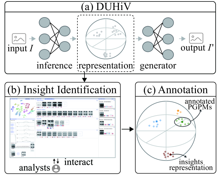
Figure 1: The pipeline of our method. (a) A DenseU-Hierarchical VAE (DUHiV) model used to learn the representation of PGPMs. (b) A visual interface used to visualize the learned representations, identify insights and generate representations for insights. (c) An annotation module that compares the representations of PGPMs and insights.

This paper presents the following contributions:

• We design a new hierarchical VAE architecture, DUHiV, that achieves a significantly tighter evidence lower bound (ELBO).

• We develop a visual interface that efficiently supports interactive insight identification by conducting arithmetic operations on the learned representations.

• We propose effective unsupervised and semi-supervised multi-label annotation methods used for annotating the dataset with identified insights.

2 Problem Definition

Let $\mathcal{G}=\{v_{1},v_{2},...,v_{M}\}$ be a bus set of size $M$. The set of PGPMs is denoted as $\mathcal{I}=\{I_{1},I_{2},...,I_{N}\}$, where each $I_{i}$ represents an PGPM, showing the voltage variation of the buses $\mathcal{G}$ in a period of time. Figure 4 (a) provides an example set $\mathcal{I}$ of PGPMs. The horizontal axis of each PGPM represents time and the vertical axis represents buses $\mathcal{G}$, sorted by their ID. The voltage values are depicted by the grayscale of pixels. We focus our study on variable voltage because it is one of the most significant and affected variables in TSA problems Kundur et al. (2004). In fact, our work can be extended to PGPMs of other variables like frequency and rotor angle.

A TSA insight refers to certain interesting facts extracted from a PGPM $I_{i}$ and is defined as follows:

Definition (TSA insight) A TSA insight is the variable variations in a subset $\widehat{\mathcal{G}}$ of $\mathcal{G}$ from a start time to an end time. Such variations can be periodic, correlated and anomalous, etc..

The objective is to (i) identify a TSA insight set $A=\{a_{1},a_{2},...,a_{K}\}$ in $\mathcal{I}$ and (ii) perform multi-label annotation on the dataset by constructing a vector $Y_{i}=\{a^{i}_{1},a^{i}_{2},...,a^{i}_{K}\}$ for each $I_{i}$ where $a^{i}_{j}\in Y_{i}$ is assigned as 1 if insight $j$ is identified in $I_{i}$ and 0 otherwise, denoted as $R=(I_{i},Y_{i})^{N}_{i=1}$.

3 Methodology

3.1 DenseU-Hierarchical VAE (DUHiV)

We design DenseU-Hierarchical VAE (DUHiV) to learn the representation of PGPMs. Following the architecture presented in Rezende et al. (2014), we achieve further improvement by using dense block Huang et al. (2017) in the inference process and a symmetric U-Net expanding path Ronneberger et al. (2015) in the generative process to capture the hierarchical structure of latent variables and accommodate the large size of PGPMs. We design two hierarchies consisting of 2 layers and 4 layers of latent variables respectively for two datasets of different sizes. (Section 4.1). The network architecture of the 2-layer DUHiV is presented in Figure 2.

DUHiV assumes that a given PGPM, denoted as $\mathbf{x}$, can be represented by a set of latent variables $\mathbf{z}$, from which something very similar to $\mathbf{x}$ can be reconstructed. Therefore, DUHiV simultaneously trains an inference model, which learns the posterior distribution $q_{\phi}(\mathbf{z}|\mathbf{x})$ of latent variables, and a generative model $p_{\theta}(\mathbf{x},\mathbf{z})$$=p_{\theta}(\mathbf{x}|\mathbf{z})p_{\theta}(\mathbf{z})$, which reconstructs $\mathbf{x}$, by maximizing the likelihood:

$$p_{\theta}(\mathbf{x})=\int_{z}p_{\theta}(\mathbf{x},\mathbf{z})dz,$$ (1)

as well as minimizing the Kullback-Leibler divergence between the inferenced posterior distribution $q_{\phi}(\mathbf{z}|\mathbf{x})$ and the groundtruth distribution $p(\mathbf{z}|\mathbf{x})$:

$$KL(q_{\phi}(\mathbf{z}|\mathbf{x})\|p(\mathbf{z}|\mathbf{x})).$$ (2)

In the generative model $p_{\theta}$, the latent variables $\mathbf{z}$ are split into $L$ layers $\mathbf{z}_{i},i=1,\ldots L$ , and the generative process is described as follows:

$$\vspace{-2mm}\begin{split}\vspace{-2mm}p(\mathbf{z})&=\Pi_{i=1}^{L}p(\mathbf{z}_{i}),p(\mathbf{z}_{i})\mathcal{N}(0,I),i\in 1,\ldots,L\\ q_{\phi}(\mathbf{z}|\mathbf{x})&=\Pi_{i=1}^{L}q_{\phi}(\mathbf{z}_{i}|\mathbf{x}),q_{\phi}(\mathbf{z}_{i}|\mathbf{x})=\mathcal{N}(\boldsymbol{\mu}_{i}(\mathbf{x}),\boldsymbol{\Sigma}_{i}(\mathbf{x})),\\ p_{\theta}(\mathbf{x},\mathbf{z})&=p_{\theta}(\mathbf{x}|\mathbf{z})p(\mathbf{z}),p_{\theta}(\mathbf{x}|\mathbf{z})=\mathcal{N}(g_{\theta}(\mathbf{z}_{1},\ldots,\mathbf{z}_{L}),\sigma^{2}),\\ \end{split}$$

where $g_{\theta}(\mathbf{z}_{1},\ldots,\mathbf{z}_{L})$ is a deterministic function. The variational principle provides a tractable evidence lower bound (ELBO) by combining Eqs. (1) and (2):

$$\vspace{-2mm}\begin{split}\mathcal{L}(\theta,\phi,\mathbf{x})&=\log(p_{\theta}(\mathbf{x}))-KL(q_{\phi}(\mathbf{z}|\mathbf{x})\|p(\mathbf{z}|\mathbf{x}))\\ &=E_{q_{\phi}(\mathbf{z}|\mathbf{x})}[\log p_{\theta}(\mathbf{x}|\mathbf{z})]-KL(q_{\phi}(\mathbf{z}|\mathbf{x})\|p(\mathbf{z})),\end{split}$$ (3)

which is estimated by reparameterization tricks and sampling  Kingma and Welling (2013) and is written in a closed form:

$$\begin{split}\hat{\mathcal{L}}(\theta,\phi,\mathbf{x})=\frac{1}{K}\sum_{k=1}^{K}-\frac{\|\mathbf{x}-g_{\theta}(\mathbf{z}_{1}^{k},\ldots,\mathbf{z}_{L}^{k})\|_{2}^{2}}{\sigma^{2}}+\\ \sum_{l=1}^{L}[\|\boldsymbol{\mu}_{l}\|_{2}^{2}+trace(\boldsymbol{\Sigma}_{l})-\log|\boldsymbol{\Sigma}_{l}|].\end{split}\vspace{-2mm}$$ (4)

Specifically, we take the learned posterior distribution $q_{\phi}(\mathbf{z}|\mathbf{x})$ of latent variables from the inference model as the representation.

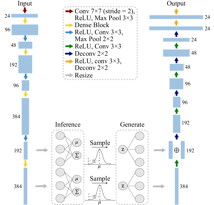
Figure 2: The DUHiV architecture with two layers of latent variables. The dense block is used in the inference process (left) and the U-Net is used in the generative process (right). The posterior distribution of the hierarchical latent variables are inferenced by fully connection layers (middle).

3.2 Interactive Insight Identification

We perform arithmetic operations on representations of PGPMs derived from DUHiV and develop visualization-based approaches to analyze the semantic changes of the reconstructed PGPM brought by such operations. In this way, we interactively identify an insight set $A=\{a_{1},a_{2},...,a_{K}\}$ and generate the representation for each insight in it, denoted as $P=\{\mathbf{p}_{1},\mathbf{p}_{2},...,\mathbf{p}_{K}\}$ where $\mathbf{p}_{i}$ corresponds to the representation of insight $a_{i}$. Specifically, we address the following tasks which is beyond the capability of automatic methods:

T1. Understand the landscape of the latent space. For a reasonable representation, variations of different latent variables are expected to result in different semantic changes of the reconstructed PGPM. We allow users to walk in the latent space by flexibly adjusting all latent variables and observe the reconstructed PGPM. This helps users to decide which latent variables need to be adjusted to define an appropriate representation of a TSA insight.

T2. Generate the representation $\mathbf{p}_{i}$ for a TSA insight $a_{i}$. We provide an efficient definition strategy based on arithmetic operations between representation vectors. Three types of operations are supported. The first operation is the most direct and intuitive way. Given a PGPM $I_{i}$ and its representation $p(\mathbf{z}|I_{i})$, the value of each latent variable $z_{i}$ is randomly sampled and flexibly adjusted (Figure 3 (B1)). The second operation is to perform linear interpolation between the representations of a given PGPMs pair $(I_{i},I_{j})$ (Figure 3 (B2)). The last one is to perform addition and subtraction operations to existing representations (Figure 3 (B3)), which is the most efficient way among all operations.

The Visual Interface. Figure 3 illustrates the visualization interface, consisting of five components (A-E). The projection view (A) is the entrance of the interface, in which PGPMs $\mathcal{I}$ is projected to a two-dimensional space using t-distributed Stochastic Neighbor Embedding (t-SNE) and clustered using Kmeans clustering. We use 2-Wasserstein distance to compute the distance between two distributions $I_{i}\sim\mathcal{N}(\boldsymbol{\mu}_{i},\boldsymbol{\Sigma}_{i})$ and $I_{j}\sim\mathcal{N}(\boldsymbol{\mu_{j}},\boldsymbol{\Sigma}_{j})$:

$$W_{2}(p_{i},p_{j})=\|\boldsymbol{\mu}_{i}-\boldsymbol{\mu}_{j}\|^{2}_{2}+tr(\boldsymbol{\Sigma}_{i}+\boldsymbol{\Sigma}_{j}-2(\boldsymbol{\Sigma}^{1/2}_{j}\boldsymbol{\Sigma}_{i}\boldsymbol{\Sigma}^{1/2}_{j})^{1/2}).$$ (5)

To avoid visual occlusion and preserve the overall distribution of $\mathcal{I}$ as much as possible, we exploit blue noise sampling on $\mathcal{I}$ and only project the sampled ones. Users start interacting with the interface by selecting clusters of interest and displaying them in the cluster view (C). For a selected cluster, we display the PGPMs on the right and display the average PGPM of this cluster on the left. The average PGPM is generated by reconstructing from the average representation. Then users select PGPMs in the cluster view and perform the three type of arithmetic operations in the control panel (B), as mentioned in T2. Specifically, interpolation between $I_{i}\sim\mathcal{N}(\boldsymbol{\mu}_{i},\boldsymbol{\Sigma}_{i})$ and $I_{j}\sim\mathcal{N}(\boldsymbol{\mu}_{j},\boldsymbol{\Sigma}_{j})$ is computed as:

$$\vspace{-2mm}I_{t}\sim\mathcal{N}(t\boldsymbol{\mu}_{i}+(1-t)\boldsymbol{\mu}_{j},(t\boldsymbol{\Sigma}^{1/2}_{i}+(1-t)\boldsymbol{\Sigma}^{1/2}_{j})^{2}),$$ (6)

where $t\in[0,1]$ and $I_{t}$ equals to $I_{i}$ and $I_{j}$ when t=1 and 0, respectively. The interpolation parameters can be flexibly adjusted in the interface. After arithmetic operations, we generate representation vectors and display them in the analysis view (D) together with the corresponding reconstructed PGPM. The representation vector is displayed by heatmap, in which the color of each block indicates the sample value of a latent variable, with bluer color indicates lower value and redder indicates higher value. When a generated representation is selected to represent a TSA insight, it is recorded in the insight view (E). Its heatmap and reconstructed PGPM are displayed. Users can also add descriptions to it.

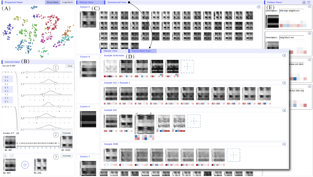
Figure 3: The visual interface used to present and analyze the representation of TSA Insights. (A) The projection view that projects PGPMs to a two-dimensional space. (B) The control panel supports arithmetic operations. (C) The cluster view shows original PGPMs for the selected clusters. (D) The analysis view shows semantic changes brought by arithmetic operations on representations. (E) The insight view records the identified insights.

Generating an Insight Representation. With the support of the visual interface, defining an insight representation is done in three steps.

First, we need to identify an interested insight $a_{i}$. The visual interface provides two efficient ways to do this. One is to observe the PGPMs of a selected cluster and discover an insight existing in most of them. The other is to observe outliers of a cluster and analyze whether a special insight exists.

Second, we need to define the representation for $a_{i}$. We can generate representations by using the three type of arithmetic operations and observe changes in the reconstructed PGPM. The $\mathbf{p}_{i}$ is determined when its reconstructed PGPM contains and only contains $a_{i}$.

Finally, we record the representation $\mathbf{p}_{i}$ and add descriptions to it. By iteratively repeating this process, we finally obtain an insight set $A=\{a_{1},a_{2},...,a_{K}\}$ and its corresponding representation set $P=\{\mathbf{p}_{1},\mathbf{p}_{2},...,\mathbf{p}_{K}\}$.

3.3 Insight Annotation

Based on the outputs of Section 3.1 and Section 3.2, we propose two methods to annotate the dataset $\mathcal{I}$ with insight labels in $A$.

Semi-supervised Method In the semi-supervised way, we identify insights $A$ but do not necessarily generate representations $P$ for them. Instead, users manually annotate part of the dataset directly with the identified insight categories during the exploration process. The rest of the dataset is then automatically annotated in a semi-supervised way in which the DUHiV model learns from the unlabeled data and classifies on the labeled data.

Unsupervised Method In the unsupervised way, we use the previously identified insight set $A$ and the generated representation set $P$. We annotate the dataset $\mathcal{I}$ by computing the similarity between each $\mathbf{p}_{i}$ and each PGPM $I_{i}$. In our experiment, we compute the Euclidean distance between $\mathbf{p}_{i}$ and the representation vector of $I_{i}$, which is sampled by taking the mean of every marginal distribution in $q_{\phi}(\mathbf{z}|\mathbf{I})$. Therefore, for each $I_{i}$, we yield a similarity vector $s_{i}=[s_{i}^{1},...,s_{i}^{K}]$, where $s_{i}^{j}$ representing the probability of annotating $I_{i}$ with insight $a_{j}$ and higher $s_{i}^{j}$ indicates higher probability.

4 Evaluation

We conduct three experiments on two real-world PGPM datasets. The first demonstrates the superiority of the DUHiV architecture over other hierarchical VAEs. The second presents qualitative case studies to show the effectiveness of the identification process in our visual interface. The last evaluates the annotation accuracy of our framework. We first introduce our test datasets and then explain our experiments.

4.1 Data Description

We evaluate our method on two real-world PGPM datasets. The first dataset contains 3,504 PGPMs, denoted as PGPM-3K. The size of each PGPM is $368\times 464$, from a small-size power grid in Northern China that contains 368 buses and is simulated at 464 time points. The time interval between adjacent time points is 0.01 second. The grayscale of pixel $(i,j)$ depicts the voltage value of bus $i$ at time $j$. The second dataset is in the same form with the first one. It contains 250,925 PGPMs, denoted as PGPM-250k, whose size is $800\times 640$. The time interval between adjacent time points is 0.03 second.

Specifically, PGPM-3K is manually labeled with 10 labels in cooperation with domain experts from China Electric Power Research Institute (CEPRI). On average, each PGPM is annotated with approximately 2.5 labels. Considering it is extremely time-consuming to label PGPM-250k, quantitative experiments are only performed on PGPM-3K.

4.2 Sample Generation Performance

We conduct the first experiment on PGPM-3Kn and compare DUHiV with two hierarchical VAE models with MLP architectures, that is, Deep Latent Gaussian Models Rezende et al. (2014) (DLGM) and Ladder VAE Sønderby et al. (2016) (LVAE). Specifically, we compare samples of generated PGPMs and the evidence lower bound (ELBO) which is widely used VAE models Kingma and Welling (2013).

Experimental Settings. For fair comparison, we fine-tune the parameters of all models to achieve best performance on our dataset. For DUHiV, we choose design parameters via empirical validations. Specifically, we use DenseNet-121 Huang et al. (2017) as the structure of the inference net and use a hierarchy of two layers of latent variables of sizes 8 and 8. The model is trained for 1200 epochs using Stochastic gradient descent (SGD) with momentum 0.9 and the batch size is 144. The initial learning rate is set to 0.005. The decay of learning rate is set to 0.9 every 10 epoch after the first 800 epochs and is set to 0.9 every epoch after the next 200 epochs. We also use the warm-up strategy in Sønderby et al. (2016) during the first 300 epochs of training. For DLGM, we use a model consisting of two deterministic layers of 400 hidden units and two stochastic layers of 8 latent variables as used in the NORB object recognition dataset. For LVAE, the implemented model consists of two MLPs of size 512 and 256, and two stochastic layers of 8 latent variables.

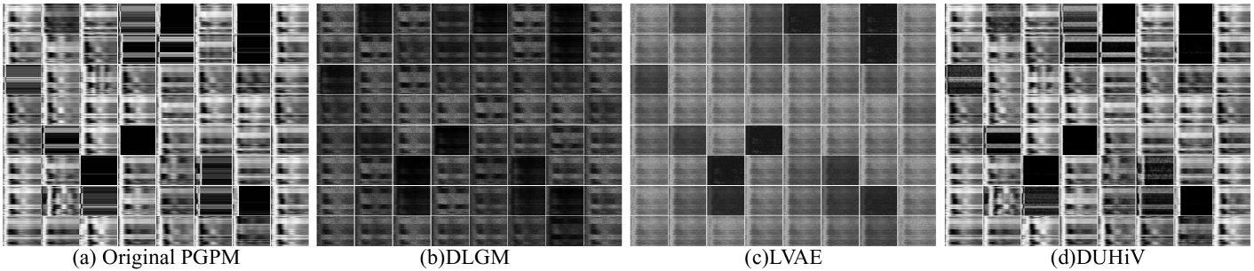
Figure 4: samples generated from PGPM-3K by DLGM (b), LVAE (c) and DUHiV (d).

Results. We present samples generated by the three models from the original PGPMs in Figure 4. As shown, LVAE captures hue features but filtered out contour information, while DLGM only captures shape features. Instead, DUHiV captures more comprehensive features and therefore achieves the best generation result. The evidence lower bound (ELBO) on the train and test sets in Table 1 also shows significantly performance improvement of DUHiV over DLGM and LVAE. All these improvements indicates the superiority of our DenseU architecture than the commonly-used MLPs structure over two aspects. First, U-Net extracts features of different levels, including low-level visual patterns and high-level semantic correspondence. Second, the dense block ensures the difference of these features. Therefore, the higher-quality PGPMs generated by DUHiV can further enhance the efficiency and effectiveness of insight identification in our visual interface.

Model	$\leq log(p(x))$
	Train	Test
DLGM	-25627.5	-25520.0
LVAE	-13630.9	-13624.3
DUHiV	-2345.4	-2416.5

Table 1: Comparison results of evidence lower bound (ELBO) of our method and the representative VAE models on PGPM-3K. The best results are marked in bold.

4.3 Insigt Identification

We conduct the second experiment on both PGPM-3K and PGPM-250K to demonstrate the effectiveness of our method in TSA insight identification.

Figure 5 shows example PGPMs reconstructed from the TSA insight representations. By interacting with our visual interface, we can decompose an original PGPM into a combination of several insights, generate a representation for each insight, and use the representation to reconstruct the PGPM. The reconstructed PGPM are inevitably blurry to some extent because it is not necessarily in the generation space of the dataset. Despite the blur, we can notice that the reconstructed PGPM successfully captures the main features of an insight.

Take insight $a$ in Figure 5 as an example, we explain how we define its representation with the support of the visual interface. We use the two-layer hierarchy of latent variables of sizes 8 and 8. Latent variables in the second layer determine the overall insight and the semantic correspondence, and the ones in the first layer determine detailed local shape. So we decide to first adjust the second layer to obtain the target insight and then adjust the first layer for local optimization. Particularly, different latent variables in the second layer determine different aspects of the generated PGPM: the hue, the horizontal/vertical position, the width/height of the insight, etc.. As shown, insight $a$ represents the sudden increase of voltage shortly after the start time. An intuitive way to define the representation of insight $a$ is to start from the corresponding original PGPM and remove the four black blocks. Therefore, we first adjust the latent variable controlling the hue in the second layer, then adjust the first layer to form a clearer shape and finally obtain an effective representation.

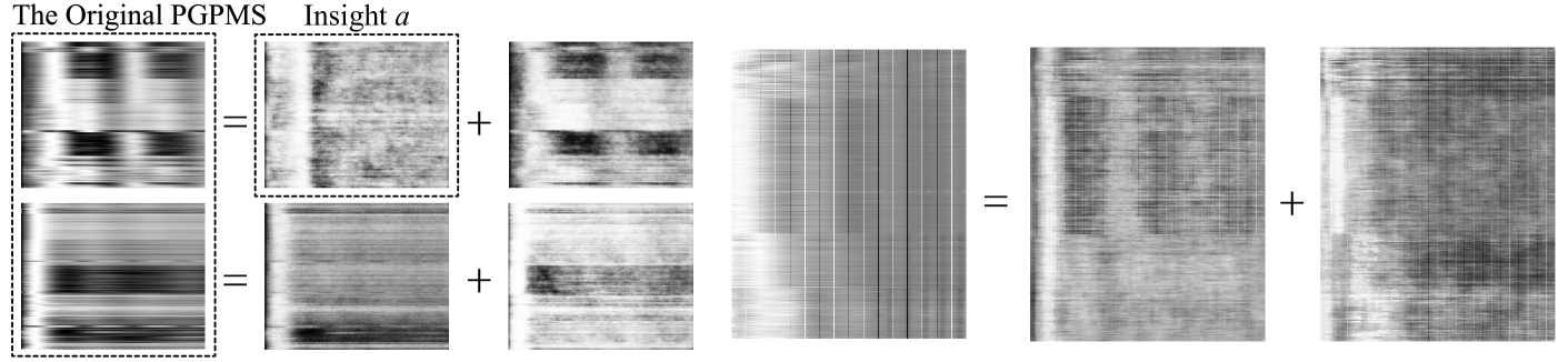
Figure 5: Reconstructed PGPMs of TSA insights. Left: PGPM-3K. Right: PGPM-250K.

4.4 Insight Annotation

We conduct the last experiment on PGPM-3K. We apply DUHiV as a feature extractor and compare it with other three unsupervised representation learning models: Non-Parametric Instance Discrimination Wu et al. (2018) (NPID) which is the state-of-the-art on ImageNet classification, and DLGM, LVAE in Section 4.2. We demonstrate the quality of the learned features by evaluating the annotation performance using these features. Specifically, we use average precision (AP) and mean average precision (mAP), which are widely used in multi-label learning algorithms Li et al. (2012). For fair comparison, We use the same DenseNet-121Huang et al. (2017) as the CNN backbone for NPID. Other experimental settings are the same with Section 4.2.

Semi-supervised Method. For fair comparison, we build KNN classifiers using the learned representations for all models to annotate the dataset. We perform 5-fold cross validation on PGPM-3K. The proportion of the labeled dataset varies from $1\%$ to $100\%$ of the entire dataset. Figure 6 shows that DUHiV and DLGM outperform LVAE and NPID by a large margin. The trivial performance of LVAE is because it captures shape features only (Section 4.2). Therefore, DLGM can achieve better mAP with tighter ELBO than LVAE. We also notice that when $10\%$ of the dataset is labeled, DUHiV can achieve a $81.03\%$ mAP, which is only $10.7\%$ less than the $100\%$-labeled situation. This advantage can significantly reduce annotation cost and demonstrates superiority over NPID which is sensitive to the annotation proportion.

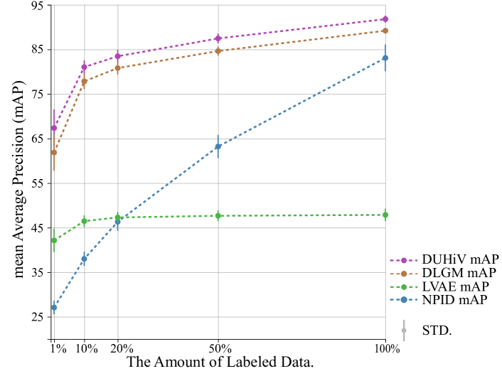
Figure 6: Comparison Results of mean Accuracy (mA) and mean Average Precision (mAP) in automatic mode with an increasing fraction of labeled data (x axis).

Unsupervised Method. For fair comparison, we interactively identify insights by using DUHiV and use all models to learn the features of the reconstructed PGPMs of the identified insights. We report the 5-fold cross validation results in Table 2. As shown, our method achieves the best mAP of $64.4\%$, leading to a nearly $38.7\%$ performance improvement over NPID, $34.1\%$ improvement over LVAE and $15.4\%$ improvement over DLGM. To be noticed, the unsupervised interactive mode enables accurate annotation by achieving comparable mAP to the semi-supervised automatic mode with $1\%$ labeled data. It indicates that with the support of our visual interface, the generated representations of insights are effective enough to approach a ground-truth level.

Model	P1	P2	P3	P4	P5	P6	P7	P8	P9	P10	mAP
DLGM	98.9$\pm$0.3	64.9$\pm$4.8	70.2$\pm$1.7	33.9$\pm$4.4	34.9$\pm$2.0	45.5$\pm$5.9	32.2$\pm$9.1	48.6$\pm$2.8	29.9$\pm$1.8	31.3$\pm$6.3	49.0$\pm$1.1
LVAE	46.9$\pm$16.5	20.9$\pm$2.3	32.7$\pm$7.8	23.9$\pm$1.1	62.3$\pm$6.6	16.6$\pm$2.6	35.7$\pm$1.7	19.7$\pm$2.3	38.6$\pm$2.7	6.1$\pm$2.4	30.3$\pm$2.7
NPID	26.0$\pm$4.9	20.1$\pm$2.5	24.3$\pm$2.0	22.7$\pm$2.1	53.0$\pm$2.6	14.7$\pm$2.4	32.1$\pm$3.5	17.7$\pm$2.4	35.4$\pm$3.8	10.9$\pm$7.1	25.7$\pm$1.4
our method	72.5$\pm$3.9	71.0$\pm$5.0	77.3$\pm$2.5	38.4$\pm$7.4	80.7$\pm$3.5	50.8$\pm$6.3	73.2$\pm$7.2	64.8$\pm$7.3	49.7$\pm$5.9	66.2$\pm$6.9	64.4$\pm$1.1

Table 2: Comparison results of AP and mAP in $\%$ of our method and the baselines on the PGPM-3K dataset (mean $\pm$ std.). Column P$i$ indicates the category of insight $i$. The best results are marked in bold.

5 Related Work

Automatic Insight Identification. Insights, in the sense of knowledge discovery and data mining, are interesting facts underly the data Lin et al. (2018). To accelerate and simplify the tedious insight identification process, KDD experts achieve automatic insight identification by storing data in a specified data structure, for example, a data cube, and applying approximate query processing techniques to speed up the query Lin et al. (2018); Tang et al. (2017). In this paper, we extend this concept to data in the form of chart images and adopt deep learning techniques to achieve efficient interactive insight identification.

Chart Image Recognition. Existing chart image recognition mainly focuses on two tasks: chart type classification and visual contents decoding Mishchenko and Vassilieva (2011). Insight identification shares a common framework with these two tasks that starts from feature extraction and ends at insight extraction. For the feature extraction part, prior models use hand-crafted features Savva et al. (2011) but does not scale well with large amount of unbalanced data. Amara et. al. Amara et al. (2017) leverage convolutional neural network (CNN) on image sets and achieve better classification results. Different from these methods, our method supports unsupervised feature extraction and arithmetic feature operations to generate higher-quality features. For the insight extraction part, existing works mainly rely on supervised classification or unsupervised clustering which output label numbers instead of semantic insights. In contrast, we adopt visualization-based approaches to interactively and directly define and extract insights based on the learned representations.

Disentangled Representation Learning. Disentanglement requires different independent variables in the learned representation to capture independent factors that generate the input data. Early methods are based on denoising autoencoders Kingma and Welling (2013) and restricted Boltzmann machines Hinton et al. (2006). However, deep generative models, represented by variational autoencoder (VAE) Maaløe et al. (2015) and generative adversarial net (GAN) Goodfellow et al. (2014), have recently achieved better results in this area due to their ability in preserving all factors of variation Tschannen et al. (2018). Mathieu et. al. Mathieu et al. (2016) introduce a conditional generative model that leverages both VAE and GAN. Their model learns to separate the factors related to labels from another source of variability based on weak assumptions. InfoGAN Chen et al. (2016) makes a further progress by training without any kind of supervision. Being an information-theoretic extension to GAN, it maximizes the mutual information between subsets of latent variables and the observation. The main drawback of these approaches is the lack of interpretability between latent variables and aspects of the generated image. In contrast, we follow  Rezende et al. (2014) and  Sønderby et al. (2016) to build a novel hierarchical VAE architecture to ease this problem by building hierarchies of latent variables.

6 Conclusion

In this paper, we propose an interactive insight identification and annotation framework for transient stability insight discovery in power grid pixel maps. We develop a DenseU-hierarchical variational autoencoder combined with interactive visualization-based approaches for representation learning of transient stability insights. To the best of our knowledge, this is the first work on interactive insight identification and annotation in power grid images and also on learning more refined representations of insights. Experiments using real-world datasets indicate the improvement of our method compared to baselines.

References

- Amara et al. [2017] Jihen Amara, Pawandeep Kaur, Michael Owonibi, and Bassem Bouaziz. Convolutional neural network based chart image classification. 2017.
- Chen et al. [2016] Xi Chen, Yan Duan, Rein Houthooft, John Schulman, Ilya Sutskever, and Pieter Abbeel. Infogan: Interpretable representation learning by information maximizing generative adversarial nets. In Advances in Neural Information Processing Systems 29: Annual Conference on Neural Information Processing Systems 2016, December 5-10, 2016, Barcelona, Spain, pages 2172–2180, 2016.
- Goodfellow et al. [2014] Ian J. Goodfellow, Jean Pouget-Abadie, Mehdi Mirza, Bing Xu, David Warde-Farley, Sherjil Ozair, Aaron C. Courville, and Yoshua Bengio. Generative adversarial nets. In Advances in Neural Information Processing Systems 27: Annual Conference on Neural Information Processing Systems 2014, December 8-13 2014, Montreal, Quebec, Canada, pages 2672–2680, 2014.
- Hinton et al. [2006] Geoffrey E. Hinton, Simon Osindero, and Yee Whye Teh. A fast learning algorithm for deep belief nets. Neural Computation, 18(7):1527–1554, 2006.
- Huang et al. [2017] Gao Huang, Zhuang Liu, Laurens van der Maaten, and Kilian Q. Weinberger. Densely connected convolutional networks. In 2017 IEEE Conference on Computer Vision and Pattern Recognition, CVPR 2017, Honolulu, HI, USA, July 21-26, 2017, pages 2261–2269, 2017.
- Kafle et al. [2018] Kushal Kafle, Brian L. Price, Scott Cohen, and Christopher Kanan. DVQA: understanding data visualizations via question answering. In 2018 IEEE Conference on Computer Vision and Pattern Recognition, CVPR 2018, Salt Lake City, UT, USA, June 18-22, 2018, pages 5648–5656, 2018.
- Kingma and Welling [2013] Diederik P. Kingma and Max Welling. Auto-encoding variational bayes. CoRR, abs/1312.6114, 2013.
- Kundur et al. [2004] Prabha Kundur, John Paserba, Venkat Ajjarapu, Göran Andersson, Anjan Bose, Claudio Canizares, Nikos Hatziargyriou, David Hill, Alex Stankovic, Carson Taylor, et al. Definition and classification of power system stability. IEEE transactions on Power Systems, 19(2):1387–1401, 2004.
- Li et al. [2012] Yu-Feng Li, Ju-Hua Hu, Yuan Jiang, and Zhi-Hua Zhou. Towards discovering what patterns trigger what labels. In Proceedings of the Twenty-Sixth AAAI Conference on Artificial Intelligence, July 22-26, 2012, Toronto, Ontario, Canada., 2012.
- Lin et al. [2018] Qingwei Lin, Weichen Ke, Jian-Guang Lou, Hongyu Zhang, Kaixin Sui, Yong Xu, Ziyi Zhou, Bo Qiao, and Dongmei Zhang. Bigin4: Instant, interactive insight identification for multi-dimensional big data. In Proceedings of the 24th ACM SIGKDD International Conference on Knowledge Discovery & Data Mining, KDD 2018, London, UK, August 19-23, 2018, pages 547–555, 2018.
- Maaløe et al. [2015] Lars Maaløe, Casper Kaae Sønderby, Søren Kaae Sønderby, and Ole Winther. Improving semi-supervised learning with auxiliary deep generative models. In NIPS Workshop on Advances in Approximate Bayesian Inference, 2015.
- Mathieu et al. [2016] Michaël Mathieu, Junbo Jake Zhao, Pablo Sprechmann, Aditya Ramesh, and Yann LeCun. Disentangling factors of variation in deep representation using adversarial training. In Advances in Neural Information Processing Systems 29: Annual Conference on Neural Information Processing Systems 2016, December 5-10, 2016, Barcelona, Spain, pages 5041–5049, 2016.
- Mishchenko and Vassilieva [2011] Ales Mishchenko and Natalia Vassilieva. Chart image understanding and numerical data extraction. In Sixth IEEE International Conference on Digital Information Management, ICDIM 2011, Melbourne, Australia, September 26-28, 2011, pages 115–120, 2011.
- Rezende et al. [2014] Danilo Jimenez Rezende, Shakir Mohamed, and Daan Wierstra. Stochastic backpropagation and approximate inference in deep generative models. In Proceedings of the 31th International Conference on Machine Learning, ICML 2014, Beijing, China, 21-26 June 2014, pages 1278–1286, 2014.
- Ronneberger et al. [2015] Olaf Ronneberger, Philipp Fischer, and Thomas Brox. U-net: Convolutional networks for biomedical image segmentation. In Medical Image Computing and Computer-Assisted Intervention - MICCAI 2015 - 18th International Conference Munich, Germany, October 5 - 9, 2015, Proceedings, Part III, pages 234–241, 2015.
- Savva et al. [2011] Manolis Savva, Nicholas Kong, Arti Chhajta, Fei-Fei Li, Maneesh Agrawala, and Jeffrey Heer. Revision: automated classification, analysis and redesign of chart images. In Proceedings of the 24th Annual ACM Symposium on User Interface Software and Technology, Santa Barbara, CA, USA, October 16-19, 2011, pages 393–402, 2011.
- Sønderby et al. [2016] Casper Kaae Sønderby, Tapani Raiko, Lars Maaløe, Søren Kaae Sønderby, and Ole Winther. Ladder variational autoencoders. In Advances in Neural Information Processing Systems 29: Annual Conference on Neural Information Processing Systems 2016, December 5-10, 2016, Barcelona, Spain, pages 3738–3746, 2016.
- Tang et al. [2017] Bo Tang, Shi Han, Man Lung Yiu, Rui Ding, and Dongmei Zhang. Extracting top-k insights from multi-dimensional data. In Proceedings of the 2017 ACM International Conference on Management of Data, SIGMOD Conference 2017, Chicago, IL, USA, May 14-19, 2017, pages 1509–1524, 2017.
- Tschannen et al. [2018] Michael Tschannen, Olivier Bachem, and Mario Lucic. Recent advances in autoencoder-based representation learning. CoRR, abs/1812.05069, 2018.
- Wong et al. [2009] Pak Chung Wong, Kevin Schneider, Patrick Mackey, Harlan Foote, George Chin Jr., Ross T. Guttromson, and Jim Thomas. A novel visualization technique for electric power grid analytics. IEEE Trans. Vis. Comput. Graph., 15(3):410–423, 2009.
- Wu et al. [2018] Zhirong Wu, Yuanjun Xiong, Stella X. Yu, and Dahua Lin. Unsupervised feature learning via non-parametric instance discrimination. In 2018 IEEE Conference on Computer Vision and Pattern Recognition, CVPR 2018, Salt Lake City, UT, USA, June 18-22, 2018, pages 3733–3742, 2018.
- Yan et al. [2015] Jun Yan, Yufei Tang, Haibo He, and Yan Sun. Cascading failure analysis with dc power flow model and transient stability analysis. IEEE Transactions on Power Systems, 30(1):285–297, 2015.