Volumetric Capture of Humans with a Single RGBD Camera via
Semi-Parametric Learning

Abstract

Volumetric (4D) performance capture is fundamental for AR/VR content generation. Whereas previous work in 4D performance capture has shown impressive results in studio settings, the technology is still far from being accessible to a typical consumer who, at best, might own a single RGBD sensor. Thus, in this work, we propose a method to synthesize free viewpoint renderings using a single RGBD camera. The key insight is to leverage previously seen “calibration” images of a given user to extrapolate what should be rendered in a novel viewpoint from the data available in the sensor. Given these past observations from multiple viewpoints, and the current RGBD image from a fixed view, we propose an end-to-end framework that fuses both these data sources to generate novel renderings of the performer. We demonstrate that the method can produce high fidelity images, and handle extreme changes in subject pose and camera viewpoints. We also show that the system generalizes to performers not seen in the training data. We run exhaustive experiments demonstrating the effectiveness of the proposed semi-parametric model (i.e. calibration images available to the neural network) compared to other state of the art machine learned solutions. Further, we compare the method with more traditional pipelines that employ multi-view capture. We show that our framework is able to achieve compelling results, with substantially less infrastructure than previously required.

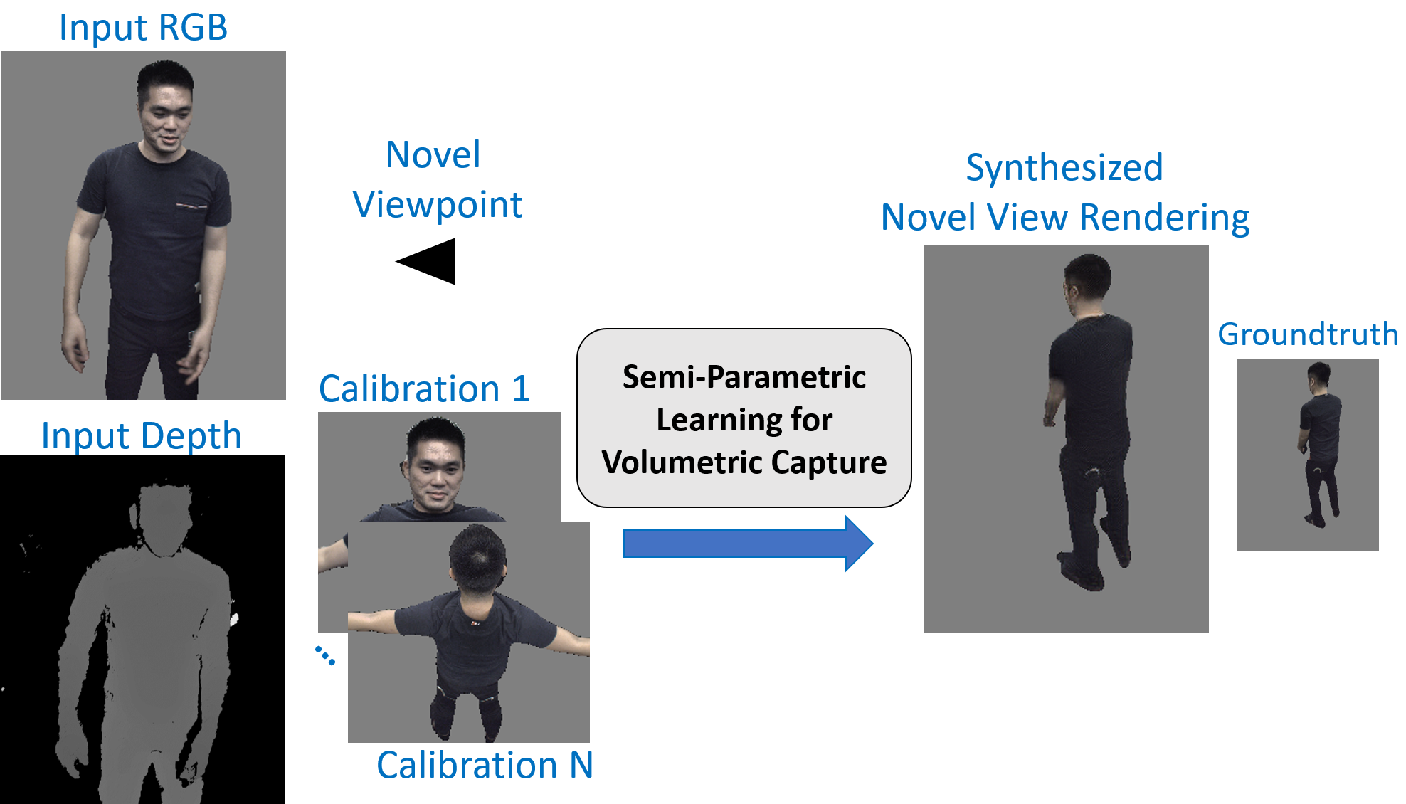
Figure 1: We propose a novel formulation to synthesize volumetric renderings of human from arbitrary viewpoints. Our system combines previously seen observations of the user (calibration images) with the current RGBD image. Given an arbitrary camera position we can generate images of the performer handling different user poses and generalizing to unseen subjects.

1 Introduction

The rise of Virtual and Augmented Reality has increased the demand for high quality 3D content to create compelling user experiences where the real and virtual world seamlessly blend together. Object scanning techniques are already available for mobile devices [30], and they are already integrated within AR experiences [20]. However, neither the industrial nor the research community have yet been able to devise practical solutions to generate high quality volumetric renderings of humans.

At the cost of reduced photo-realism, the industry is currently overcoming the issue by leveraging “cartoon-like” virtual avatars. On the other end of the spectrum, complex capture rigs [7, 39, 3] can be used to generate very high quality volumetric reconstructions. Some of these methods [8, 18] are well established, and lie at the foundation of special effects in many Hollywood productions. Despite their success, these systems rely on high-end, costly infrastructure to process the high volume of data that they capture. The required computational time of several minutes per frame make them unsuitable for real-time applications. Another way to capture humans is to extend real-time non-rigid fusion pipelines [35, 23, 44, 45, 22] to multi-view capture setups [12, 36, 11]. However, the results still suffer from distorted geometry, poor texturing and inaccurate lighting, making it difficult to reach the level of quality required in AR/VR applications [36]. Moreover, these methods rely on multi-view capture rigs that require several ($\approx$ 4-8) calibrated RGBD sensors.

Conversely, our goal is to make the volumetric capture technology accessible through consumer level hardware. Thus, in this paper, we focus on the problem of synthesizing volumetric renderings of humans. Our goal is to develop a method that leverages recent advances in machine learning to generate 4D videos using as little infrastructure as possible – a single RGBD sensor. We show how a semi-parametric model, where the network is provided with calibration images, can be used to render an image of a novel viewpoint by leveraging the calibration images to extrapolate the partial data the sensor can provide. Combined with a fully parametric model, this produces the desired rendering from an arbitrary camera viewpoint; see Fig. 1.

In summary, our contribution is a new formulation of volumetric capture of humans that employs a single RGBD sensor, and that leverages machine learning for image rendering. Crucially, our pipeline does not require complex infrastructure typically required by 4D video capture setups.

We perform exhaustive comparisons with machine learned, as well as traditional state-of-the-art capture solutions, showing how the proposed system generates compelling results with minimal infrastructure requirements.

2 Related work

Capturing humans in 3D is an active research topic in the computer vision, graphics, and machine learning communities. We categorize related work into three main areas that are representative of the different trends in the literature: image-based rendering, volumetric capture, and machine learning solutions.

Image based rendering

Despite their success, most of methods in this class do not infer a full 3D model, but can nonetheless generate renderings from novel viewpoints. Furthermore, the underlying 3D geometry is typically a proxy, which means they cannot be used in combination with AR/VR where accurate, metric reconstructions can enable additional capabilities. For example, [9, 21], create impressive renderings of humans and objects, but with limited viewpoint variation. Modern extensions [1, 41] produce $360^{\circ}$ panoramas, but with a fixed camera position. The method of Zitnick et al. [50] infers an underlying geometric model by predicting proxy depth maps, but with a small $30^{\circ}$ coverage, and the rendering heavily degrades when the interpolated view is far from the original. Extensions to these methods [14, 4, 47] have attempted to circumvent these problems by introducing an optical flow stage warping the final renderings among different views, but with limited success.

Volumetric capture

Commercial volumetric reconstruction pipelines employ capture studio setups to reach the highest level of accuracy [7, 39, 12, 11, 36]. For instance, the system used in [7, 39], employs more than $100$ IR/RGB cameras, which they use to accurately estimate depth, and then reconstruct 3D geometry [27]. Non-rigid mesh alignment and further processing is then performed to obtain a temporally consistent atlas for texturing. Roughly 28 minutes per frame are required to obtain the final 3D mesh. Currently, this is the state-of-the-art system, and is employed in many AR/VR productions. Other methods [51, 35, 12, 11, 36, 13], further push this technology by using highly customized, high speed RGBD sensors. High framerate cameras [16, 15, 46] can also help make the non-rigid tracking problem more tractable, and compelling volumetric capture can be obtained with just 8 custom RGBD sensors rather than hundreds [28]. However these methods still suffer from both geometric and texture aberrations, as demonstrated by Dou et al. [11] and Du et al. [13].

Machine learning techniques

The problem of generating images of an object from novel viewpoints can also be cast from a machine learning, as opposed to graphics, standpoint. For instance, Dosovitskiy et al. [10] generates re-renderings of chairs from different viewpoints, but the quality of the rendering is low, and the operation is specialized to discrete shape classes. More recent works [25, 38, 49] try to learn the 2D-3D mapping by employing some notion of 3D geometry, or to encode multiview-stereo constraints directly in the network architecture [17]. As we focus on humans, our research is more closely related to works that attempt to synthesize 2D images of humans [48, 2, 43, 32, 31, 34, 5]. These focus on generating people in unseen poses, but usually from a fixed camera viewpoint (typically frontal) and scale (not metrically accurate). The coarse-to-fine GANs of [48] synthesizes images that are still relatively blurry. Ma et al. [31] detects pose in the input, which helps to disentangle appearance from pose, resulting in improved sharpness. Even more complex variants [32, 43] that attempt to disentangle pose from appearance, and foreground from background, still suffer from multiple artifacts, especially in occluded regions. A dense UV map can also be used as a proxy to re-render the target from a novel viewpoint [34], but high-frequency details are still not effectively captured. Of particular relevance is the work by Balakrishnan et al. [2], where through the identification and transformation of body parts results in much sharper images being generated. Nonetheless, note how this work solely focuses on frontal viewpoints.

Our approach

In direct contrast, our goal is to render a subject in unseen poses and arbitrary viewpoints, mimicking the behavior of volumetric capture systems. The task at hand is much more challenging because it requires disentangling pose, texture, background and viewpoint simultaneously. This objective has been partially achieved by Martin-Brualla et al. [33] by combining the benefits of geometrical pipelines [11] to those of convolutional architectures [42]. However, their work still necessitates a complete mesh being reconstructed from multiple viewpoints. In contrast, our goal is to achieve the same level of photo-realism from a single RGBD input. To tackle this, we resort to a semi-parametric approach [40], where a calibration phase is used to acquire frames of the users appearance from a few different viewpoints. These calibration images are then merged together with the the current view of the user in an end-to-end fashion. We show that the semi-parametric approach is the key to generating high quality, 2D renderings of people in arbitrary poses and camera viewpoints.

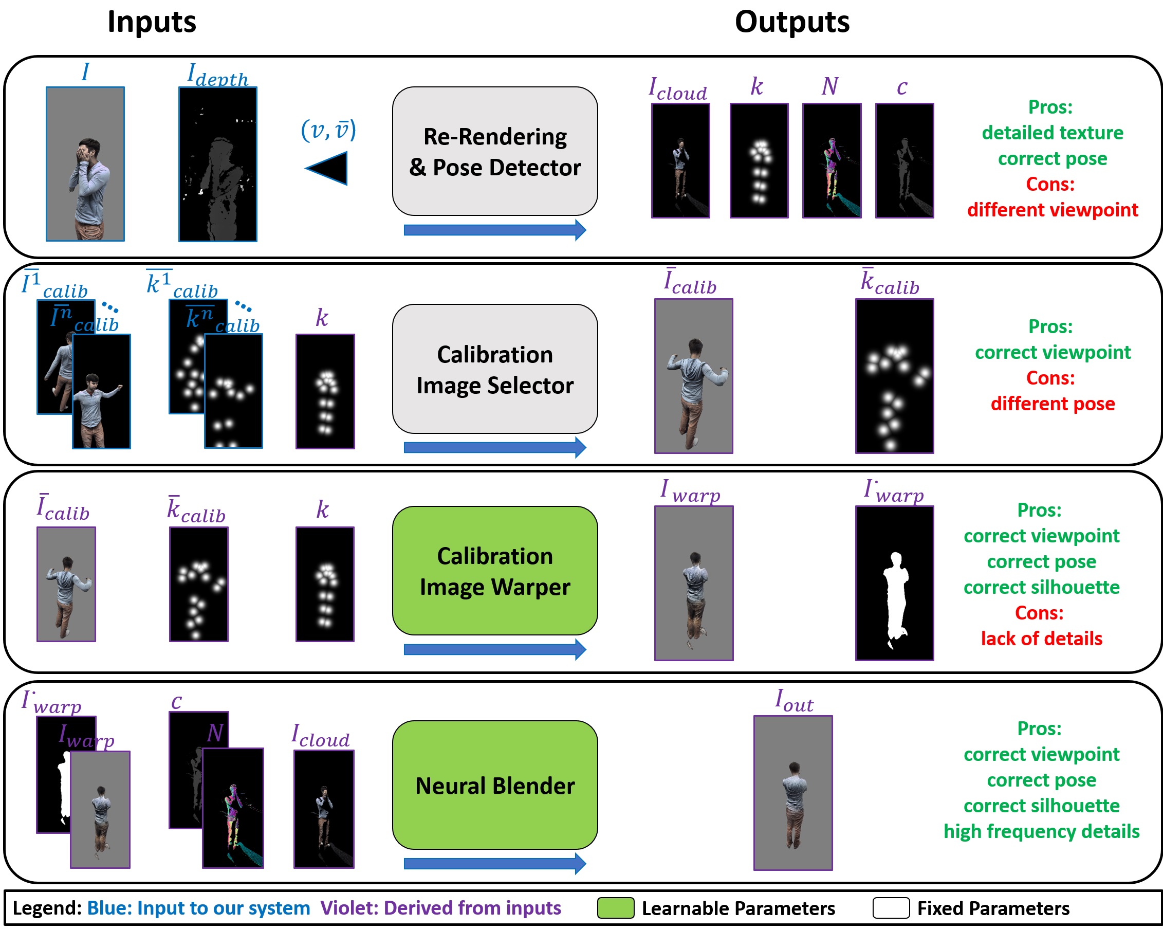
Figure 2: Proposed framework – We take in input the current RGBD image, a novel viewpoint and a collection of images acquired in a calibration stage, which depict the users in different poses observed from several viewpoints. The Re-rendering & pose-detector projects the texture using depth information and re-project back to the final viewpoint, together with the target pose. We also compute a confidence score of the current observations with respect to the novel viewpoint. This score is encoded in the normal map ${N}$ and the confidence ${c}$. The Calibration Image Selector picks the closest image (in terms of viewpoint) from a previously recorded calibration bank. The Calibration Image Warper tries to align the selected calibration image with the current pose, it also produces a silhouette mask. The Neural Blender combines the information from the warped RGB image, aligned calibration image, silhouette image and viewpoint confidence to recover the final, highly detailed RGB image.

3 Proposed Framework

As illustrated in Figure 1, our method receives as input: 1) an RGBD image from a single viewpoint, 2) a novel camera pose with respect to the current view and 3) a collection of a few calibration images observing the user in various poses and viewpoints. As output, it generates a rendered image of the user as observed from the new viewpoint. Our proposed framework is visualized in Figure 2, and includes the four core components outlined below.

Re-rendering & Pose Detector:

from the RGBD image $\bar{I}$ captured from a camera $\bar{v}$, we re-render the colored depthmap from the new camera viewpoint ${v}$ to generate an image ${I}_{\text{cloud}}$, as well as its approximate normal map ${N}$. Note we only re-render the foreground of the image, by employing a fast background subtraction method based on depth and RGB as described in [15]. We also estimate the pose ${\kappa}$ of the user, i.e. keypoints, in the coordinate frame of ${v}$, as well as a scalar confidence ${c}$, measuring the divergence between the camera viewpoints:

$$I_{\text{cloud}},{\kappa},{N},{c}=\mathcal{R}{}(\bar{I},\bar{v},{v}).$$ (1)

Calibration Image Selector:

from the collection of calibration RGBD images and poses $\{\bar{I}_{\text{calib}}^{n},\bar{\kappa}_{\text{calib}}^{n}\}$, we select one that best resembles the target pose ${\kappa}$ in the viewpoint ${v}$:

$$\bar{I}_{\text{calib}},\bar{\kappa}_{\text{calib}}=\mathcal{S}{}(\{\bar{I}_{\text{calib}}^{n},\bar{\kappa}_{\text{calib}}^{n}\},{\kappa}).$$ (2)

Calibration Image Warper:

given the selected calibration image $\bar{I}_{\text{calib}}$ and the user’s pose $\bar{\kappa}_{\text{calib}}$, a neural network $\mathcal{W}$ with learnable parameters ${\omega}$ warps this image into the desired pose ${\kappa}$, while simultaneously producing the silhouette mask ${I}^{\bullet}_{\text{warp}}$ of the subject in the new pose:

$${I}_{\text{warp}},{I}^{\bullet}_{\text{warp}}=\mathcal{W}_{\omega}{}(\bar{I}_{\text{calib}},\bar{\kappa}_{\text{calib}},{\kappa}).$$ (3)

Neural Blender:

finally, we blend the information captured by the traditional re-rendering in (1) to the warped calibration image (3) to produce our final image $I_{out}$:

$$I_{out}=\mathcal{B}_{{\beta}}({I}_{\text{cloud}},{I}_{\text{warp}},{I}^{\bullet}_{\text{warp}},{N},{c}).$$ (4)

Note that while (1) and (2) are not learnable, they extract quantities that express the geometric structure of the problem. Conversely, both warper (3) and (4) are differentiable and trained end-to-end where the loss is the weighted sum between warper $\mathcal{L}_{\text{warper}}$ and blender $\mathcal{L}_{\text{blender}}$ losses. The weights $\omega_{\text{warper}}$ and $\omega_{\text{blender}}$ are chosen to ensure similar contributions between the two. We now describe each component in details, motivating the design choices we took.

3.1 Re-rendering & Pose Detector

We assume that camera intrinsic parameters (optical center $\mathbf{o}$ and focal length $\mathbf{f}$) are known and thus the function $\Pi^{-1}(\mathbf{p},z|\mathbf{o},\mathbf{f}):\mathbb{R}{}^{3}\mapsto\mathbb{R}{}^{3}$ maps a 2D pixel $\mathbf{p}=(x,y)$ with associated depth $z$ to a 3D point in the local camera coordinate frame.

Rendering $\rightarrow I_{\text{cloud}}$

Via the function $\Pi^{-1}$, we first convert the depth channel of $\bar{I}$ into a point cloud of size $M$ in matrix form as $\bar{\mathbf{P}}\!\in\!\mathbb{R}^{4\times M}$. We then rotate and translate this point cloud into the novel viewpoint coordinate frame as ${\mathbf{P}}=\mathbf{T}\bar{\mathbf{P}}$, where $\mathbf{T}\!\in\!\mathbb{R}^{4\times 4}$ is the homogeneous transformation representing the relative transformation between $\bar{v}$ and ${v}$. We render ${\mathbf{P}}$ to a 2D image $I_{\text{cloud}}$ in OpenGL by splatting each point with a $3\times 3$ kernel to reduce re-sampling artifacts. Note that when input and novel camera viewpoints are close, i.e. $\bar{v}\sim{v}$, then $I_{out}\sim I_{\text{cloud}}$, while when $\bar{v}\nsim{v}$ then $I_{\text{cloud}}$ would mostly contain unusable information.

Pose detection $\rightarrow{\kappa}$

We also infer the pose of the user by computing 2D keypoints $\bar{\kappa}_{\text{2D}}=\mathcal{K}_{\gamma}(\bar{I})$ using the method of Papandre et al. [37] where $\mathcal{K}$ is a pre-trained feed-forward network. We then lift 2D keypoints to their 3D counterparts $\bar{\kappa}$ by employing the depth channel of $\bar{I}$ and, as before, transform them in the camera coordinate frame ${v}$ as ${\kappa}$. We extrapolate missing keypoints when possible relying on the rigidity of the limbs, torso, face, otherwise we simply discard the frame. Finally, in order to feed the keypoints ${\kappa}$ to the networks in (3) and (4) following the strategy in [2]: we encode each point in an image channel (for a total of $17$ channels) as a Gaussian centered around the point with a fixed variance. We tried other representations, such as the one used in [43], but found that the selected one lead to more stable training.

Confidence and normal map $\rightarrow{c},{N}$

In order for (4) to determine whether a pixel in image $I_{\text{cloud}}$ contains appropriate information for rendering from viewpoint $v$ we provide two sources of information: a normal map and a confidence score. The normal map ${N}$, processed in a way analogous to $I_{\text{cloud}}$, can be used to decide whether a pixel in $\bar{I}$ has been well observed from the input measurement $\bar{v}$ (e.g. the network should learn to discard measurements taken at low-grazing angles). Conversely, the relationship between $\bar{v}$ and ${v}$, encoded by ${c}$, can be used to infer whether a novel viewpoint is back-facing (i.e. ${c}<0$) or front-facing it (i.e. ${c}>0$). We compute this quantity as the dot product between the cameras view vectors: ${c}=[0,0,1]\cdot{\mathbf{r}_{z}}/{\|\mathbf{r}_{z}\|}$, where $\bar{v}$ is always assumed to be the origin and $\mathbf{r}_{z}$ is the third column of the rotation matrix for the novel camera viewpoint ${v}$. An example of input and output of this module can be observed in Figure 2, top row.

3.2 Calibration Image Selector

In a pre-processing stage, we collect a set of calibration images $\{\bar{I}_{\text{calib}}^{n}\}$ from the user with associated poses $\{\bar{\kappa}_{\text{calib}}^{n}\}$ . For example, one could ask the user to rotate in front of the camera before the system starts; an example of calibration set is visualized in the second row of Figure 2. While it is unreasonable to expect this collection to contain the user in the desired pose, and observed exactly from the viewpoint ${v}$, it is assumed the calibration set will contain enough information to extrapolate the appearance of the user from the novel viewpoint ${v}$. Therefore, in this stage we select a reasonable image from the calibration set that, when warped by (3) will provide sufficient information to (4) to produce the final output. We compute a score for all the calibration images, and the calibration image with the highest score is selected. A few examples of the selection process are shown in the supplementary material. Our selection score is composed of three terms:

$$S^{n}=\omega_{\text{head}}S_{\text{head}}^{n}+\omega_{\text{torso}}S_{\text{torso}}^{n}+\omega_{\text{sim}}S_{\text{sim}}^{n}$$ (5)

From the current 3D keypoints ${\kappa}$, we compute a 3D unit vector representing the forward looking direction of the user’s head. The vector is computed by creating a local coordinate system from the keypoints of the eyes and nose. Analogously, we compute 3D unit vectors $\{d^{n}_{\text{calib}}\}$ from the calibration images keypoints $\{\bar{\kappa}_{\text{calib}}^{n}\}$. The head score is then simply the dot product $S^{n}_{\text{head}}=d\cdot d^{n}_{\text{calib}}$, and a similar process is adopted for $S_{\text{torso}}^{n}$, where the coordinate system is created from the left/right shoulder and the left hip keypoints. These two scores are already sufficient to accurately select a calibration image from the desired novel viewpoint, however they do not take into account the configuration of the limbs. Therefore we introduce a third term, $S_{\text{sim}}^{n}$, that computes a similarity score between the keypoints $\bar{\kappa}_{\text{calib}}^{n}$ in the calibration images to those in the target pose ${\kappa}$. To simplify the notation, we refer to $\hat{\kappa}$ and $\hat{\kappa}^{n}_{\text{calib}}$ as the image-space 2D coordinates of keypoints in homogeneous coordinates. We can compute a similarity transformation (rotation, translation, scale) $\mathbf{T}_{n}\!\in\!\mathbb{R}^{3\times 3}$ that aligns the two sets. Note that at least $2$ points are needed to estimate our $4$ DOF transformation (one for rotation, two for translation, and one for scale), therefore we group arm keypoints (elbow, wrist) and leg keypoints (knee, foot) together. For instance, for all the keypoints belonging to the left arm group ($LA$) we calculate:

$$\arg\min_{\mathbf{T}_{n}^{LA}}\sum_{LA}\|\hat{\kappa}^{LA}-\mathbf{T}_{n}^{LA}\hat{\kappa}^{n,LA}_{\text{calib}}\|^{2}$$ (6)

We then define the similarity score as:

$$S^{LA}=\exp(-\sigma\|\hat{\kappa}-\mathbf{T}_{n}^{LA}\hat{\kappa}^{n,LA}_{\text{calib}}\|)$$ (7)

The final $S^{n}_{sim}$ is the sum of the scores for the $4$ limbs (indexed by $j$). The weights $\omega_{j}$ are tuned to give more importance to head and torso directions, which define the desired target viewpoint. The calibration image $\bar{I}_{\text{calib}}$ with the respective pose $\bar{\kappa}_{\text{calib}}$ with the highest score $\bar{S}$ is returned from this stage. All the details regarding the chosen parameters can be found in the supplementary material.

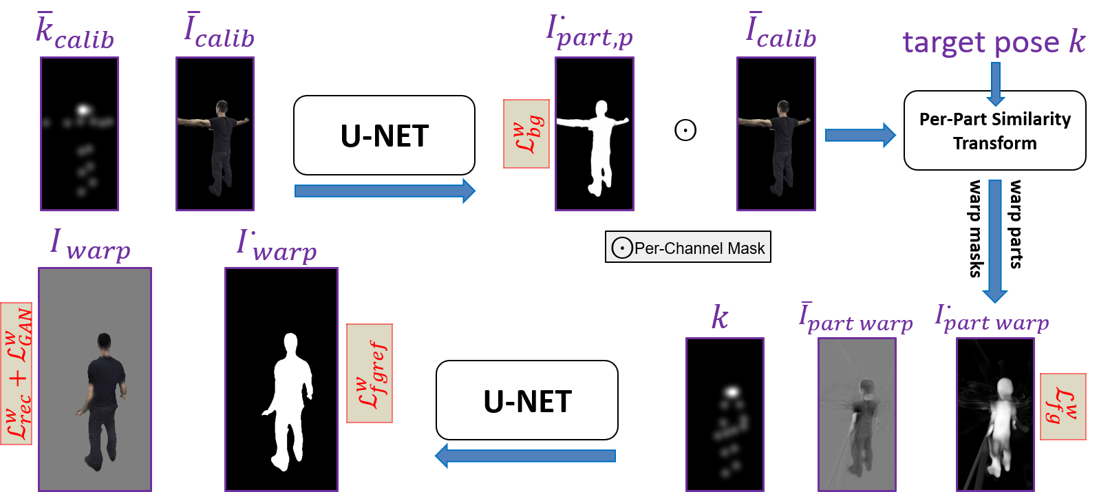
Figure 3: The Calibration Warper takes as input the selected calibration the selected calibration image $\bar{I}_{\text{calib}}$ and pose $\bar{\kappa}_{\text{calib}}$ and aligns it to the target pose ${\kappa}$. It also produces a foreground mask ${I}^{\bullet}_{\text{warp}}$. For visualization purposes multiple channels are collapsed into a single image. See text for details.

3.3 Calibration Warper

The selected calibration image $\bar{I}_{\text{calib}}$ should have a similar viewpoint to ${v}$, but the pose $\bar{\kappa}_{\text{calib}}$ could still be different from the desired ${\kappa}$, as the calibration set is small. Therefore, we warp $\bar{I}_{\text{calib}}$ to obtain an image ${I}_{\text{warp}}$, as well as its silhouette ${I}^{\bullet}_{\text{warp}}$. The architecture we designed is inspired by Balakrishnan et al. [2], which uses U-NET modules [42]; see Figure 3 for an overview.

The calibration pose $\bar{\kappa}_{\text{calib}}$ tensor ($17$ channels, one per keypoint) and calibration image $\bar{I}_{\text{calib}}$ go through a U-NET module that produces as output part masks $\{{I}^{\bullet}_{\text{part,p}}\}$ plus a background mask ${I}^{\bullet}_{\text{bg}}$. These masks select which regions of the body should be warped according to a similarity transformation. Similarly to [2], the warping transformations are not learned, but computed via (6) on keypoint groups of at least two 2D points; we have $10$ groups of keypoints (see supplementary material for details). The warped texture $\bar{I}_{\text{warp,p}}$ has $3$ RGB channels for each keypoints group $p$ ($30$ channels in total). However, in contrast to [2], we do not use the masks just to select pixels to be warped, but also warp the body part masks themselves to the target pose ${\kappa}$. We then take the maximum across all the channels and supervise the synthesis of the resulting warped silhouette $\bar{I}^{\bullet}_{\text{part warp}}$. We noticed that this is crucial to avoid overfitting, and to teach the network to transfer the texture from the calibration image to the target view and keeping high frequency details. We also differ from [2] in that we do not synthesize the background, as we are only interested in the performer, but we do additionally predict a background mask ${I}^{\bullet}_{\text{bg}}$.

Finally, the $10$ channels encoding the per-part texture $\bar{I}_{\text{warp,p}}$ and the warped silhouette mask $\bar{I}^{\bullet}_{\text{part warp}}$ go through another U-NET module that merges the per-part textures and refines the final foreground mask. Please see additional details in the supplementary material.

The Calibration Warper is training minimizing multiple losses:

$$\begin{split}\mathcal{L}_{warp}&=w_{\text{rec}}^{\mathcal{W}}\mathcal{L}_{\text{rec}}^{\mathcal{W}}+w_{\text{fg}}^{\mathcal{W}}\mathcal{L}_{\text{fg}}^{\mathcal{W}}+w_{\text{bg}}^{\mathcal{W}}\mathcal{L}_{\text{bg}}^{\mathcal{W}}+\\ &+w_{\text{fgref}}^{\mathcal{W}}\mathcal{L}_{\text{fgref}}^{\mathcal{W}}+w_{\text{GAN}}^{\mathcal{W}}\mathcal{L}_{\text{GAN}}^{\mathcal{W}},\end{split}$$ (8)

where all the weights $w^{\mathcal{W}}_{*}$ are empirically chosen such that all the losses are approximately in the same dynamic range.

Warp reconstruction loss $\mathcal{L}_{rec}^{\mathcal{W}}$

Our perceptual reconstruction loss $\mathcal{L}_{rec}^{\mathcal{W}}=\|\text{VGG}({I}_{\text{warp}})-\text{VGG}(I_{\text{gt}})\|_{2}$ measures the difference in VGG feature-space between the predicted image ${I}_{\text{warp}}$, and the corresponding groundtruth image $I_{\text{gt}}$. Given the nature of calibration images, ${I}_{\text{warp}}$ may lack high frequency details such as facial expressions. Therefore, we compute the loss selecting features from conv2 up to conv5 layers of the VGG network.

Warp background loss $\mathcal{L}_{bg}^{\mathcal{W}}$

In order to remove the background component of [2], we have a loss $\mathcal{L}_{bg}^{\mathcal{W}}=\|{I}^{\bullet}_{\text{bg}}-{I}^{\bullet}_{\text{bg,gt}}\|_{1}$ between the predicted mask ${I}^{\bullet}_{\text{bg}}$ and the groundtruth mask ${I}^{\bullet}_{\text{bg,gt}}=1-{I}^{\bullet}_{\text{gt}}$. We considered other losses (e.g. logistic) but they all produced very similar results.

Warp foreground loss $\mathcal{L}_{fg}^{\mathcal{W}}$

Each part mask is warped into target pose ${\kappa}$ by the corresponding similarity transformation. We then merge all the channels with a max-pooling operator, and retrieve a foreground mask $\bar{I}^{\bullet}_{\text{part warp}}$, over which we impose our loss $\mathcal{L}_{fg}^{\mathcal{W}}=\|\bar{I}^{\bullet}_{\text{part warp}}-{I}^{\bullet}_{\text{gt}}\|_{1}$. This loss is crucial to push the network towards learning transformation rather than memorizing the solution (i.e. overfitting).

Warp foreground refinement loss $\mathcal{L}_{fgref}^{\mathcal{W}}$

The warped part masks ${I}^{\bullet}_{\text{part,p}}$ may not match the silhouette precisely due to the assumption of similarity transformation among the body parts, therefore we also refine the mask producing a final binary image ${I}^{\bullet}_{\text{warp}}$. This is trained by minimizing the loss $\mathcal{L}_{fgref}^{\mathcal{W}}=\|{I}^{\bullet}_{\text{warp}}-{I}^{\bullet}_{\text{gt}}\|_{1}$.

Warp GAN loss $\mathcal{L}_{GAN}^{\mathcal{W}}$

We finally add a GAN component that helps hallucinating realistic high frequency details as shown in [2]. Following the original paper [19] we found more stable results when used the following GAN component: $\mathcal{L}_{GAN}^{\mathcal{W}}=-\log(D({I}^{\bullet}_{\text{warp}}))$, where the discriminator $D$ consists of $5$ conv layers with $256$ filters, with max pooling layers to downsample the feature maps. Finally we add $2$ fully connected layers with $256$ features and a sigmoid activation to produce the discriminator label.

3.4 Neural Blender

The re-rendered image $I_{\text{cloud}}$ can be enhanced by the content in the warped calibration ${I}_{\text{warp}}$ via a neural blending operation consisting of another U-NET module: please see the supplementary material for more details regarding the architecture. By design, this module should always favor details from $I_{\text{cloud}}$ if the novel camera view ${v}$ is close to the original $\bar{v}$, while it should leverage the texture in ${I}_{\text{warp}}$ for back-facing views. To guide the network towards this, we pass as input the normal map ${N}$, and the confidence ${c}$, which is passed as an extra channel to each pixel. These additional channels contain all the information needed to disambiguate frontal from back views. The mask ${I}^{\bullet}_{\text{warp}}$ acts as an additional feature to guide the network towards understanding where it should hallucinate image content not visible in the re-rendered image $I_{\text{cloud}}$.

The neural blender is supervised by the following loss:

$$\begin{split}\mathcal{L}_{blender}=w_{\text{rec}}^{\mathcal{B}}\mathcal{L}^{\mathcal{B}}_{\text{rec}}+w_{\text{GAN}}^{\mathcal{B}}\mathcal{L}^{\mathcal{B}}_{\text{GAN}}\end{split}$$ (9)

Blender reconstruction loss $\mathcal{L}^{\mathcal{B}}_{\text{rec}}$

The reconstruction loss computes the difference between the final image output $I_{out}$ and the target view $I_{\text{gt}}$ . This loss is defined $\mathcal{L}^{\mathcal{B}}_{\text{rec}}=\|\text{VGG}(I_{out})-\text{VGG}(I_{\text{gt}})\|_{2}+w_{\ell_{1}}\|I_{out}-I_{\text{gt}}\|_{1}$. A small ($w_{\ell_{1}}=0.01$) photometric ($\ell_{1}$) loss is needed to ensure faster color convergence.

Blender GAN loss $\mathcal{L}_{\text{GAN}}^{\mathcal{B}}$

This loss follows the same design of the one described for the calibration warper network.

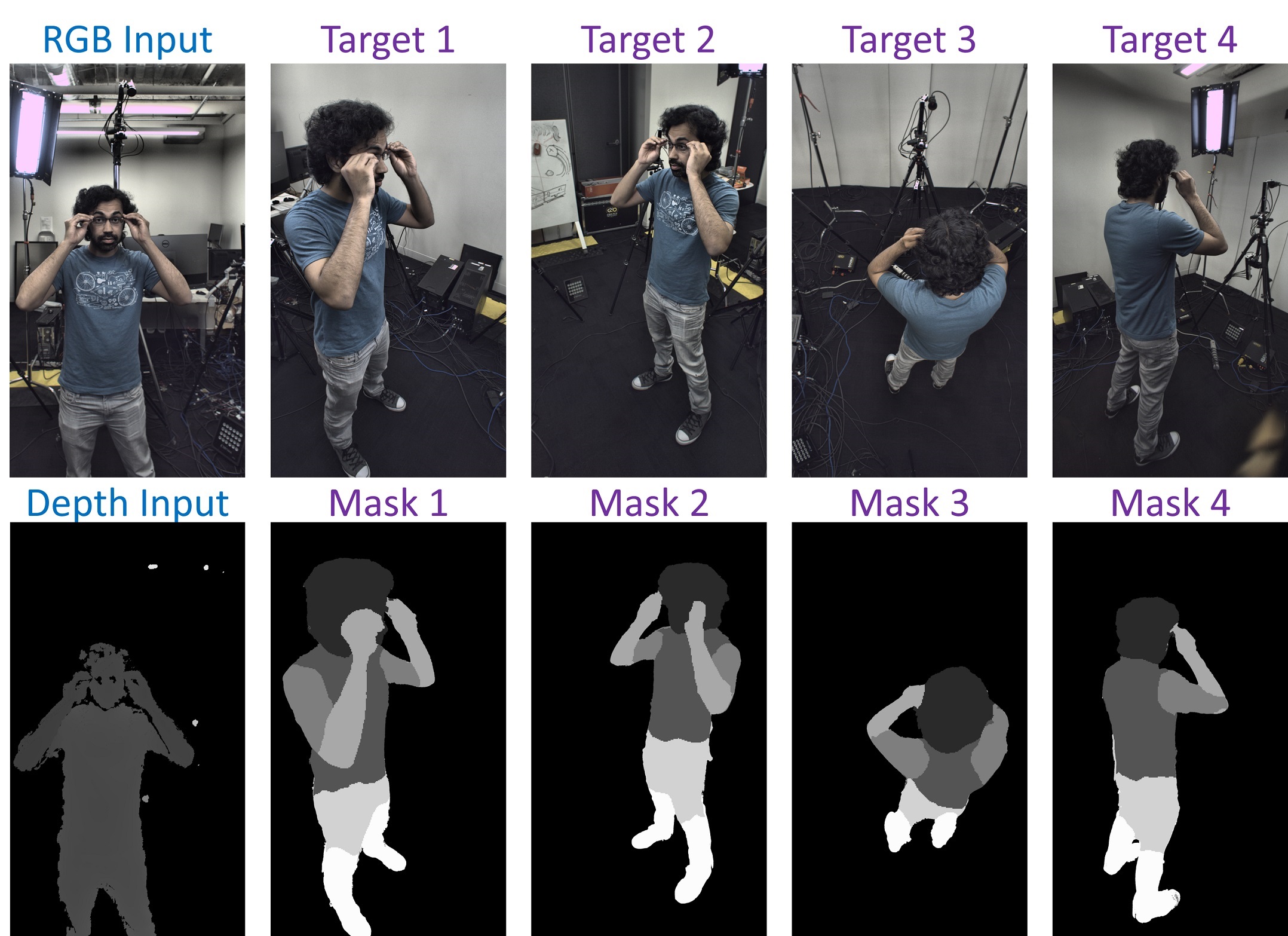
Figure 4: Examples of input RGBD and groundtruth novel views with associated masks. Note that in our dataset we have access to $8$ novel views for each input frame.

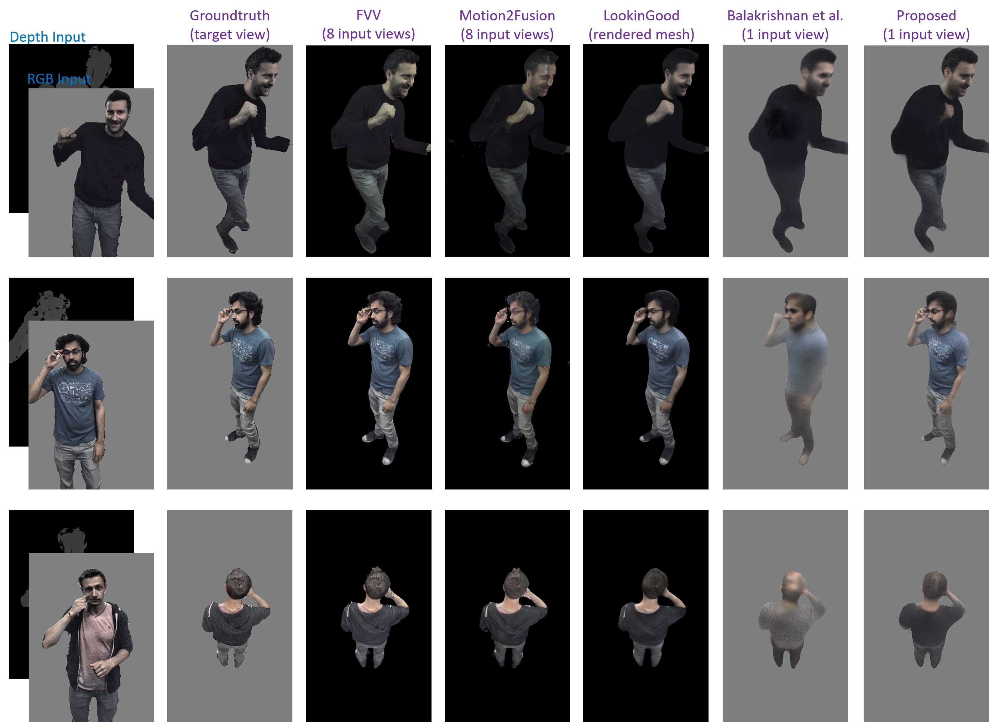
Figure 5: Comparisons with state of the art methods. Notice how the proposed framework favorably compares with traditional volumetric capture rigs that use many ($8$) cameras from multiple viewpoints. Notice that due to its real-time nature, Motion2Fusion [11] can afford only low resolution ($1280\times 1024$) RGB images for the texturing phase, whereas FVV [7] accepts as input $4000\times 3000$ images.

4 Evaluation

We now evaluate our method and compare with representative state-of-the-art algorithms. We then perform an ablation study on the main components of the system. All the results here are shown on test sequences not used during training; additional exhaustive evaluations can be found in the supplementary material.

4.1 Training Data Collection

The training procedure requires input views from an RGBD sensor and multiple groundtruth target views. Recent multi-view datasets of humans, such as Human 3.6M [24], only provides $4$ RGB views and a single low-resolution depth (TOF) sensor, which is insufficient for the task at hand; therefore we collected our own dataset with $20$ subjects. Similarly to [33], we used a multi-camera setup with $8$ high resolution RGB views coupled with a custom active depth sensor [46]. All the cameras were synchronized at at $30$Hz by an external trigger. The raw RGB resolution is $4000\times 3000$, whereas the depth resolution is $1280\times 1024$. Due to memory limitations during the training, we downsampled also the RGB images to $1280\times 1024$ pixels.

Each performer was free to perform any arbitrary movement in the capture space (e.g. walking, jogging, dancing, etc.) while simultaneously performing facial movements and expressions. For each subject we recorded $10$ sequences of $500$ frames. For each participant in the training set, we left $2$ sequences out during training. One sequence is used as calibration, where we randomly pick $10$ frames at each training iteration as calibration images. The second sequence is used as test to evaluate the performance of a seen actor but unseen actions. Finally, we left $5$ subjects out from the training datasets to assess the performances of the algorithm on unseen people.

Silhouette masks generation

As described in Sec. 3.3 and Sec. 3.4, our training procedure relies on groundtruth foreground and background masks (${I}^{\bullet}_{\text{gt}}$ and ${I}^{\bullet}_{\text{bg,gt}}=1-{I}^{\bullet}_{\text{gt}}$). Thus, we use the state-of-the-art body semantic segmentation algorithm by Chen et al. [6] to generate these masks ${I}^{\bullet}_{\text{gt}}$ which are then refined by a pairwise CRF [29] to improve the segmentation boundaries. We do not explicit make use of the semantic information extracted by this algorithm such as in [33], leaving this for future work. Note that at test time, the segmentation is not required input, but nonetheless we predict a silhouette as a by product as to remove the dependency on the background structure. Examples of our training data can be observed in Figure 4. No manual annotation is required hence data collection is fully automatic.

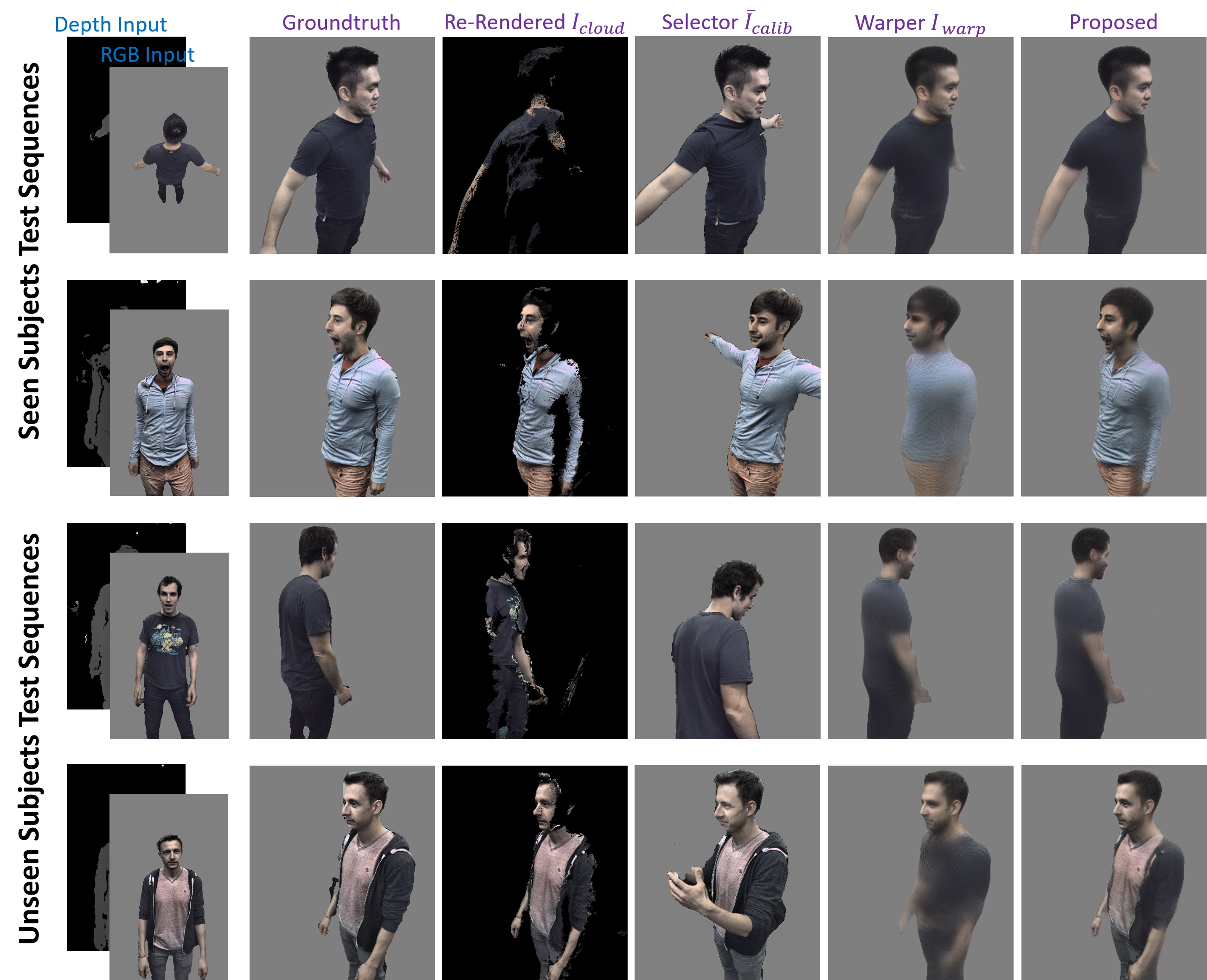
Figure 6: Results of the various stage of the pipeline. Notice how each stage of the system contributes to achieve the final high quality results, proving the effectivness of our design choices. Finally, thanks to the semi-parametric model, the algorithm generalizes well across unseen subjects.

4.2 Comparison with State of the Art

	Proposed	$I_{\text{cloud}}$	$\bar{I}_{\text{calib}}$	${I}_{\text{warp}}$	Balakrishnan et al. [2]	LookinGood  [33]	M2F [11]	FVV [7]
	1 view	1 view	1 view	1 view	1 view	8 views	8 views	8 views
$\ell_{1}$ Loss	$\mathbf{17.40}$	$27.27$	$20.02$	$18.70$	$18.01$	$38.80$	$33.72$	$\mathbf{7.39}$
PSNR	$\mathbf{28.43}$	$22.35$	$21.10$	$27.32$	$22.93$	$29.93$	$28.21$	$\mathbf{32.60}$
MS-SSIM	$\mathbf{0.92}$	$0.84$	$0.87$	$0.91$	$0.86$	$0.92$	$\mathbf{0.96}$	$\mathbf{0.96}$
VGG Loss	$\mathbf{12.50}$	$21.20$	$21.41$	$13.96$	$20.16$	$10.65$	$\mathbf{5.34}$	$6.51$

Table 1: Quantitative evaluations on test sequences. We computed multiple metrics such as Photometric Error ($\ell_{1}$ loss), PSNR, MS-SSIM and Perceptual Loss. We compared the method with the output of the rendering stage $I_{\text{cloud}}$, the output of the calibration selector $\bar{I}_{\text{calib}}$ and the output of the calibration warper ${I}_{\text{warp}}$. We also show how our method outperforms on multiple metrics the state of the art method of Balakrishna et al. [2]. We also favorably compare with full capture rig solutions such as Motion2Fusion [11], FVV [7] and the LookinGood system [33].

We now compare the method with representative state of the art approaches: we selected algorithms for comparison representative of the different strategies they use. The very recent method by Balakrishnan et al. [2] was selected as a state of the art machine learning based approach due to its high quality results. We also re-implemented traditional capture rig solutions such as FVV [7] and Motion2Fusion [11]. Finally we compare with LookinGood [33], a hybrid pipeline that combines geometric pipelines with deep networks. Notice, that these systems use all the available views ($8$ cameras in our dataset) as input, whereas our framework relies on a single RGBD view.

Qualitative Results

We show qualitative results on Figure 5. Notice how our algorithm, using only a single RGBD input, outperforms the method of Balakrishnan et al. [2]: we synthesize sharper results and also handle viewpoint and scale changes correctly. Additionally, the proposed framework generates compelling results, often comparable to multiview methods such as LookinGood [33], Motion2Fusion [11] or FVV [7].

Quantitative Comparisons

To quantitatively assess and compare the method with the state of the art, we computed multiple metrics using the available groundtruth images. The results are shown in Table 1. Our system clearly outperforms the multiple baselines and compares favorably to state of the art volumetric capture systems that use multiple input views.

4.3 Ablation Study

We now quantitatively and qualitatively analyze each each stage of the pipeline. In Figure 6 notice how each stage of the pipeline contributes to achieve the final high quality result. This proves that each component was carefully designed and needed. Notice also how we can also generalize to unseen subjects thanks to the semi-parametric approach we proposed. These excellent results are also confirmed in the quantitative evaluation we reported in Table 1: note how the output of the full system consistently outperforms the one from the re-rendering ($I_{\text{cloud}}$), the calibration image selector ($\bar{I}_{\text{calib}}$), and the calibration image warper (${I}_{\text{warp}}$). We refer the reader to the supplementary material for more detailed examples.

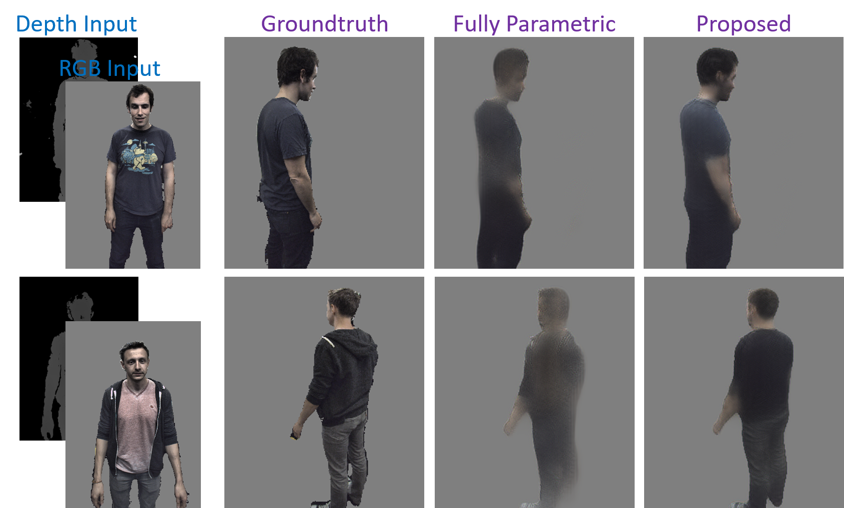
Figure 7: Comparison of the proposed system with the fully parametric model. Notice how the semi-parametric part is crucial to get the highest level of quality.

Comparison with fully parametric model

In this experiment we removed the semi-parametric part of our framework, i.e. the calibration selector and the calibration warper, and train the neural blender on the output of the re-renderer (i.e. a fully parametric model). This is similar to the approach presented in [33], applied to a single RGBD image. We show the results in Figure 7: notice how the proposed semi-parametric model is crucial to properly handle large viewpoint changes.

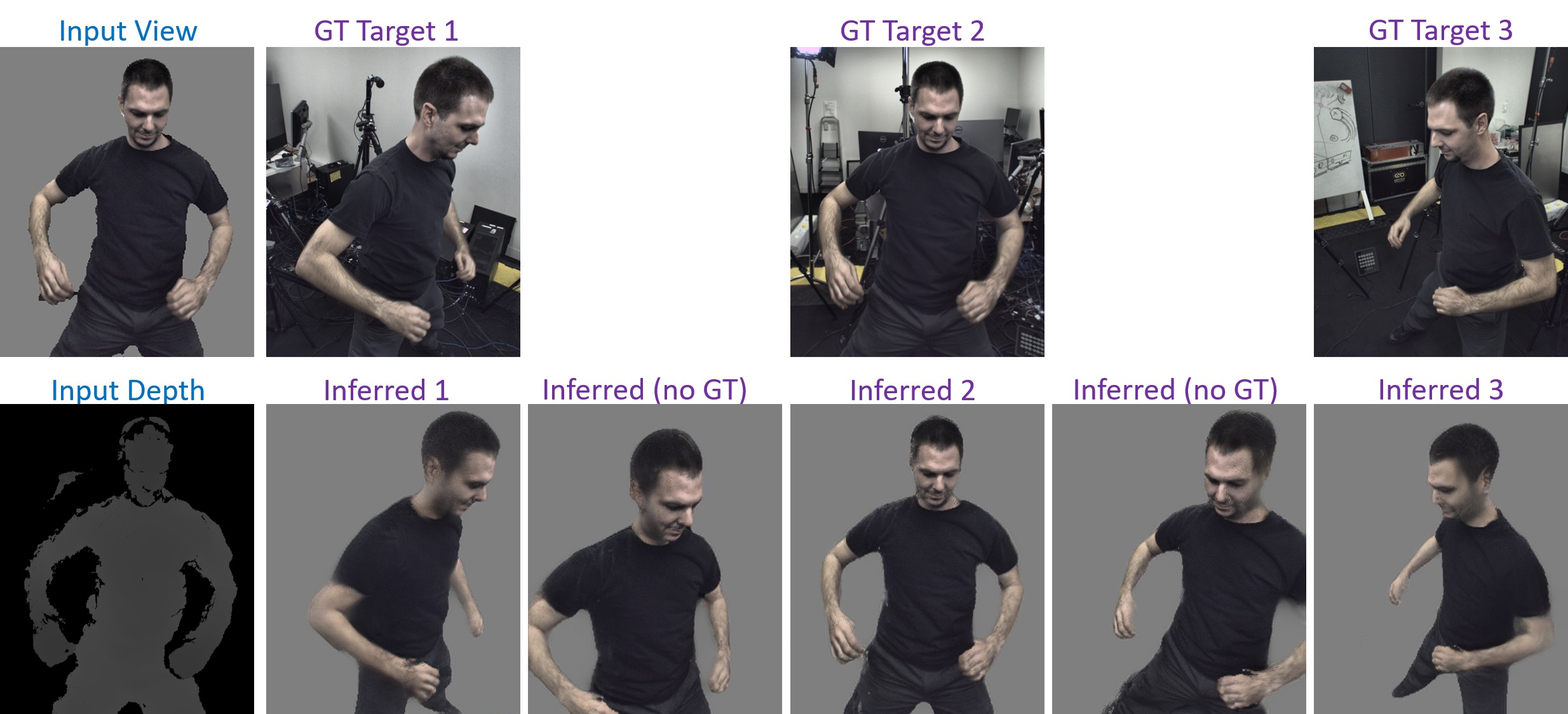
Figure 8: Predictions for viewpoints not in the training set. The method correctly infers views where no groundtruth is available.

Viewpoint generalization

We finally show in Figure 8 qualitative examples for viewpoints not present in the training set. Notice how we are able to robustly handle those cases. Please see supplementary materials for more examples.

5 Conclusions

We proposed a novel formulation to tackle the problem of volumetric capture of humans with machine learning. Our pipeline elegantly combines traditional geometry to semi-parametric learning. We exhaustively tested the framework and compared it with multiple state of the art methods, showing unprecedented results for a single RGBD camera system. Currently, our main limitations are due to sparse keypoints, which we plan to address by adding additional discriminative priors such as in [26]. In future work, we will also investigate performing end to end training of the entire pipeline, including the calibration keyframe selection and warping.

References

- [1] R. Anderson, D. Gallup, J. T. Barron, J. Kontkanen, N. Snavely, C. Hernández, S. Agarwal, and S. M. Seitz. Jump: virtual reality video. ACM TOG, 2016.
- [2] G. Balakrishnan, A. Zhao, A. V. Dalca, F. Durand, and J. V. Guttag. Synthesizing images of humans in unseen poses. CVPR, 2018.
- [3] J. Carranza, C. Theobalt, M. A. Magnor, and H.-P. Seidel. Free-viewpoint video of human actors. SIGGRAPH, 2003.
- [4] D. Casas, M. Volino, J. Collomosse, and A. Hilton. 4D Video Textures for Interactive Character Appearance. EUROGRAPHICS, 2014.
- [5] C. Chan, S. Ginosar, T. Zhou, and A. A. Efros. Everybody dance now. CoRR, 2018.
- [6] L.-C. Chen, Y. Zhu, G. Papandreou, F. Schroff, and H. Adam. Encoder-decoder with atrous separable convolution for semantic image segmentation. CoRR, abs/1802.02611, 2018.
- [7] A. Collet, M. Chuang, P. Sweeney, D. Gillett, D. Evseev, D. Calabrese, H. Hoppe, A. Kirk, and S. Sullivan. High-quality streamable free-viewpoint video. ACM TOG, 2015.
- [8] P. Debevec, T. Hawkins, C. Tchou, H.-P. Duiker, W. Sarokin, and M. Sagar. Acquiring the reflectance field of a human face. In SIGGRAPH, 2000.
- [9] P. E. Debevec, C. J. Taylor, and J. Malik. Modeling and rendering architecture from photographs: A hybrid geometry and image-based approach. In SIGGRAPH, 1996.
- [10] A. Dosovitskiy, J. T. Springenberg, M. Tatarchenko, and T. Brox. Learning to generate chairs with convolutional networks. CVPR, 2015.
- [11] M. Dou, P. Davidson, S. R. Fanello, S. Khamis, A. Kowdle, C. Rhemann, V. Tankovich, and S. Izadi. Motion2fusion: Real-time volumetric performance capture. SIGGRAPH Asia, 2017.
- [12] M. Dou, S. Khamis, Y. Degtyarev, P. Davidson, S. R. Fanello, A. Kowdle, S. O. Escolano, C. Rhemann, D. Kim, J. Taylor, P. Kohli, V. Tankovich, and S. Izadi. Fusion4d: Real-time performance capture of challenging scenes. SIGGRAPH, 2016.
- [13] R. Du, M. Chuang, W. Chang, H. Hoppe, and A. Varshney. Montage4D: Real-time Seamless Fusion and Stylization of Multiview Video Textures. Journal of Computer Graphics Techniques, 8(1), January 2019.
- [14] M. Eisemann, B. D. Decker, M. Magnor, P. Bekaert, E. D. Aguiar, N. Ahmed, C. Theobalt, and A. Sellent. Floating textures. Computer Graphics Forum, 2008.
- [15] S. R. Fanello, J. Valentin, A. Kowdle, C. Rhemann, V. Tankovich, C. Ciliberto, P. Davidson, and S. Izadi. Low compute and fully parallel computer vision with hashmatch. In ICCV, 2017.
- [16] S. R. Fanello, J. Valentin, C. Rhemann, A. Kowdle, V. Tankovich, P. Davidson, and S. Izadi. Ultrastereo: Efficient learning-based matching for active stereo systems. In CVPR, 2017.
- [17] J. Flynn, I. Neulander, J. Philbin, and N. Snavely. Deep stereo: Learning to predict new views from the world’s imagery. In CVPR, 2016.
- [18] G. Fyffe and P. Debevec. Single-shot reflectance measurement from polarized color gradient illumination. In IEEE International Conference on Computational Photography, 2015.
- [19] I. J. Goodfellow, J. Pouget-Abadie, M. Mirza, B. Xu, D. Warde-Farley, S. Ozair, A. Courville, and Y. Bengio. Generative adversarial nets. In NIPS, 2014.
- [20] Google. Arcore - google developers documentation, 2018.
- [21] S. J. Gortler, R. Grzeszczuk, R. Szeliski, and M. F. Cohen. The lumigraph. In SIGGRAPH, 1996.
- [22] K. Guo, J. Taylor, S. Fanello, A. Tagliasacchi, M. Dou, P. Davidson, A. Kowdle, and S. Izadi. Twinfusion: High framerate non-rigid fusion through fast correspondence tracking. In 3DV, 2018.
- [23] M. Innmann, M. Zollhöfer, M. Nießner, C. Theobalt, and M. Stamminger. VolumeDeform: Real-time Volumetric Non-rigid Reconstruction. In ECCV, 2016.
- [24] C. Ionescu, D. Papava, V. Olaru, and C. Sminchisescu. Human3.6m: Large scale datasets and predictive methods for 3d human sensing in natural environments. IEEE PAMI, 2014.
- [25] D. Ji, J. Kwon, M. McFarland, and S. Savarese. Deep view morphing. CoRR, 2017.
- [26] H. Joo, T. Simon, and Y. Sheikh. Total capture: A 3d deformation model for tracking faces, hands, and bodies. CVPR, 2018.
- [27] M. Kazhdan and H. Hoppe. Screened poisson surface reconstruction. ACM TOG, 2013.
- [28] A. Kowdle, C. Rhemann, S. Fanello, A. Tagliasacchi, J. Taylor, P. Davidson, M. Dou, K. Guo, C. Keskin, S. Khamis, D. Kim, D. Tang, V. Tankovich, J. Valentin, and S. Izadi. The need 4 speed in real-time dense visual tracking. SIGGRAPH Asia, 2018.
- [29] P. Krähenbühl and V. Koltun. Efficient inference in fully connected crfs with gaussian edge potentials. In NIPS, 2011.
- [30] L. Labs. 3D scanner app, 2018. https://www.3dscannerapp.com/.
- [31] L. Ma, X. Jia, Q. Sun, B. Schiele, T. Tuytelaars, and L. Van Gool. Pose guided person image generation. In NIPS, 2017.
- [32] L. Ma, Q. Sun, S. Georgoulis, L. V. Gool, B. Schiele, and M. Fritz. Disentangled person image generation. CVPR, 2018.
- [33] R. Martin-Brualla, R. Pandey, S. Yang, P. Pidlypenskyi, J. Taylor, J. Valentin, S. Khamis, P. Davidson, A. Tkach, P. Lincoln, A. Kowdle, C. Rhemann, D. B. Goldman, C. Keskin, S. Seitz, S. Izadi, and S. Fanello. Lookingood: Enhancing performance capture with real-time neuralre-rendering. In SIGGRAPH Asia, 2018.
- [34] N. Neverova, R. A. Güler, and I. Kokkinos. Dense pose transfer. ECCV, 2018.
- [35] R. A. Newcombe, D. Fox, and S. M. Seitz. Dynamicfusion: Reconstruction and tracking of non-rigid scenes in real-time. In CVPR, June 2015.
- [36] S. Orts-Escolano, C. Rhemann, S. Fanello, W. Chang, A. Kowdle, Y. Degtyarev, D. Kim, P. L. Davidson, S. Khamis, M. Dou, V. Tankovich, C. Loop, Q. Cai, P. A. Chou, S. Mennicken, J. Valentin, V. Pradeep, S. Wang, S. B. Kang, P. Kohli, Y. Lutchyn, C. Keskin, and S. Izadi. Holoportation: Virtual 3d teleportation in real-time. In UIST, 2016.
- [37] G. Papandreou, T. Zhu, N. Kanazawa, A. Toshev, J. Tompson, C. Bregler, and K. P. Murphy. Towards accurate multi-person pose estimation in the wild. CVPR, 2017.
- [38] E. Park, J. Yang, E. Yumer, D. Ceylan, and A. C. Berg. Transformation-grounded image generation network for novel 3d view synthesis. In CVPR, 2017.
- [39] F. Prada, M. Kazhdan, M. Chuang, A. Collet, and H. Hoppe. Spatiotemporal atlas parameterization for evolving meshes. ACM TOG, 2017.
- [40] X. Qi, Q. Chen, J. Jia, and V. Koltun. Semi-parametric image synthesis. CoRR, 2018.
- [41] C. Richardt, Y. Pritch, H. Zimmer, and A. Sorkine-Hornung. Megastereo: Constructing high-resolution stereo panoramas. In CVPR, 2013.
- [42] O. Ronneberger, P. Fischer, and T. Brox. U-net: Convolutional networks for biomedical image segmentation. MICCAI, 2015.
- [43] C. Si, W. Wang, L. Wang, and T. Tan. Multistage adversarial losses for pose-based human image synthesis. In CVPR, 2018.
- [44] M. Slavcheva, M. Baust, D. Cremers, and S. Ilic. Killingfusion: Non-rigid 3d reconstruction without correspondences. In CVPR, 2017.
- [45] M. Slavcheva, M. Baust, and S. Ilic. Sobolevfusion: 3d reconstruction of scenes undergoing free non-rigid motion. In CVPR, 2018.
- [46] V. Tankovich, M. Schoenberg, S. R. Fanello, A. Kowdle, C. Rhemann, M. Dzitsiuk, M. Schmidt, J. Valentin, and S. Izadi. Sos: Stereo matching in o(1) with slanted support windows. IROS, 2018.
- [47] M. Volino, D. Casas, J. Collomosse, and A. Hilton. Optimal representation of multiple view video. In BMVC, 2014.
- [48] B. Zhao, X. Wu, Z. Cheng, H. Liu, and J. Feng. Multi-view image generation from a single-view. CoRR, 2017.
- [49] T. Zhou, S. Tulsiani, W. Sun, J. Malik, and A. A. Efros. View synthesis by appearance flow. CoRR, 2016.
- [50] C. L. Zitnick, S. B. Kang, M. Uyttendaele, S. Winder, and R. Szeliski. High-quality video view interpolation using a layered representation. ACM TOG, 2004.
- [51] M. Zollhöfer, M. Nießner, S. Izadi, C. Rehmann, C. Zach, M. Fisher, C. Wu, A. Fitzgibbon, C. Loop, C. Theobalt, and M. Stamminger. Real-time non-rigid reconstruction using an rgb-d camera. ACM TOG, 2014.