The Supermarket Model with
Known and Predicted Service Times

Michael Mitzenmacher and Matteo Dell’Amico M. Mitzenmacher is with the School of Engineering and Applied Sciences, Harvard University. Email: michaelm@eecs.harvard.edu. This work was supported in part by NSF grants CCF-2101140, DMS-2023528, CCF-1563710, and CCF-1535795. M. Dell’Amico is with the University of Genoa. This work was carried out while he was with NortonLifeLock Research Group and EURECOM, France. Email: della@linux.it.

Abstract

The supermarket model refers to a system with a large number of queues, where new customers choose $d$ queues at random and join the one with the fewest customers. This model demonstrates the power of even small amounts of choice, as compared to simply joining a queue chosen uniformly at random, for load balancing systems. In this work we perform simulation-based studies to consider variations where service times for a customer are predicted, as might be done in modern settings using machine learning techniques or related mechanisms. Our primary takeaway is that using even seemingly weak predictions of service times can yield significant benefits over blind First In First Out queueing in this context. However, some care must be taken when using predicted service time information to both choose a queue and order elements for service within a queue; while in many cases using the information for both choosing and ordering is beneficial, in many of our simulation settings we find that simply using the number of jobs to choose a queue is better when using predicted service times to order jobs in a queue. In our simulations, we evaluate both synthetic and real-world workloads–in the latter, service times are predicted by machine learning. Our results provide practical guidance for the design of real-world systems; moreover, we leave many natural theoretical open questions for future work, validating their relevance to real-world situations.

Index Terms:

Supermarket model, prediction methods, scheduling, queueing analysis

1 Introduction

The success of machine learning (ML) has opened up new opportunities in terms of improving the efficiency of a wide array of processes. In this paper, we consider opportunities for using ML predictions in a specific setting: queueing in large distributed systems using the supermarket model. This also leads us to consider variants of these systems that appear to have not previously studied that do not use predictions as a starting point.

Scheduling with predicted service times is a topic of obvious practical importance for system design; however, there is a relative scarcity of studies exploring the area. We believe that this may be because the community tends to prefer analytical studies, and this particular topic appears particularly challenging to tackle analytically, even when simplifying assumptions to facilitate modeling are taken.

We take a different approach, basing our study on simulations. This choice allows us to obtain new insight that is relevant to practical system design issues. Moreover, besides using simulations based on standard distributions for queueing studies, we use real-world traces for system evaluation, where job submission time, service time, and predicted service time come from real-world systems: in particular, service time predictions are the output of a state-of-the-art approach [2].

We start with the key background. In queueing settings, the supermarket model (also described as the power of two choices, or balanced allocations) is typically described in the following way. Suppose we have a system of $n$ First In, First Out (FIFO) queues. Jobs¹¹1In this paper we use jobs instead of the more specific term customers, as the model applies to a variety of load-balancing settings. arrive to the system as a Poisson process of rate $\lambda n$ , and service times are independent and exponentially distributed with mean 1. If each job selects a random queue on arrival, then via Poisson splitting [24, Section 8.4.2] each queue acts as a standard M/M/1 queue, and in equilibrium the fraction of queues with at least $i$ jobs is $\lambda^{i}$ . Note that we consider here the tails of the queue length distribution, as it makes for easier comparisons. If each job selects two random queues on arrival, and chooses to wait at the queue with fewer customers (breaking ties randomly), then in the limiting system as $n$ grows to infinity, in equilibrium the fraction of queues with at least $i$ jobs is $\lambda^{2^{i}-1}$ . That is, the tails decrease doubly exponentially in $i$ , instead of single exponentially. In practice, even for moderate values of $n$ (say in the large hundreds), one obtains performance close to this mean field limit; this can be proven based on appropriate concentration bounds. More generally, for $d$ choices where $d$ is an integer constant greater than 1, the fraction of queues with at least $i$ jobs falls like $\lambda^{(d^{i}-1)/(d-1)}$ [21, 31]. While there are many variations on the supermarket model and its analysis (see, e.g., [1, 6, 25, 30]), here we focus on this standard, simple formulation, although we allow for general service distributions instead of just the exponential distribution.

As stated previously, here we study variations of the supermarket model where service times are predicted. To describe our work and goals, we start by considering the baseline where service times are known.

The analysis for the basic model described above assumes that service times are exponentially distributed but specific job service times are not known. (Extensions of the analysis to more general distributions are known [1, 6].) As such, an incoming job uses only the number of jobs at each chosen queue to decide which queue to join. As both a theoretical question and for possible practical implementations, it seems worthwhile to know what further improvement is possible if service times of the jobs were known.

Recently, Hellemans and Van Houdt proved results in the supermarket model setting where job reservations are made at $d$ randomly chosen queues, and once the first reservation reaches the point of obtaining service, the other reservations are canceled. This corresponds to choosing the least loaded (in terms of total remaining service time²²2We use service time and processing time interchangeably; both terms have been used historically.) of $d$ queues using FIFO queues. Their work applies to general service distributions; for the class of phase-type service distributions, they are able to express the limiting behavior of the system in terms of delayed differential equations [12]. Their results, including both theorems and simulations, show that using service time information can lead to significant improvements in the average time a job spends in the system. (The subsequent work [13] examines several additional variations.) Because of space limitations, we leave discussion of the challenges of extending these results beyond FIFO queues to Section A.1.

However, when the service times are known, there are two possible ways to potentially improve performance. First, as above, one can use the service times when selecting a queue, by choosing the least loaded queue. Second, one can order the jobs using a strategy other than FIFO; the natural strategies to minimize the average time in the system (response time) are shortest job first (SJF), preemptive shortest job first (PSJF), and shortest remaining processing time (SRPT). Here shortest job first assumes no preemption and always schedules the job with the smallest service time when a job completes, preemptive shortest job first allows preemption so that a job with a smaller service time can preempt the running job, and shortest remaining processing time allows preemption but is based on the remaining processing time instead of the total service time for a job. Note that here we assume a preempted job does not need to start from the beginning and can later continue service where it left off. Also, while apparently somewhat less natural, PSJF allows job priorities to be assigned on arrival to a queue without the need for updating, unlike SRPT.

In the setting of a single queue, Mitzenmacher has recently considered the setting where service time is predicted rather than known exactly [22]. In this model, the jobs have a joint service-predicted service density function $g(x,y)$ , where $x$ is the true service time and $y$ is the predicted service time. He provides formulae for the average time in system using corresponding strategies shortest predicted job first (SPJF), preemptive shortest predicted job first (PSPJF), and shortest predicted remaining processing time (SPRPT). Simulation results suggest that in the single queue setting even weak predictors can greatly improve performance over FIFO queues. However, using the supermarket model already provides great improvements in systems with multiple queues. It is therefore natural to consider whether predictions would still provide significant gains in the supermarket model.

The contributions of this paper include the following.

•

For the case of known service times, we provide a simulation study with synthetic traces showing the potential gains when using SJF, PSJF, and SRPT queues in the supermarket model, providing an appropriate baseline.
•

We similarly through simulations examine the benefits when only predicted information is available, using FIFO, SPJF, PSPJF, and SPRPT queues. Here we use both synthetic and real-world datasets.
•

We determine somewhat counterintuitive behaviors; for example, we find many cases where choosing the predicted least loaded queue performs worse than simply choosing the shortest queue.
•

We provide a number of open questions related to the analysis and use of these systems.

2 Additional Related Work

The supermarket model was first analyzed in the discrete settings of hashing, modeled as balls and bins processes [3, 15, 19]. It was subsequently analyzed in the setting of queueing systems, in particular in the mean field limit (also referred to as the fluid limit) as the number of queues grows to infinity [21, 31].

Ordering jobs by service time has been studied extensively in single queues. The text [11] provides an excellent introduction to the analysis of standard approaches such as SJF and SRPT in the single queue setting.

Our work falls into a recent line of work that aims to use machine learning predictions to improve traditional algorithms. For example, Lykouris and Vassilvitskii [17] show how to use prediction advice from ML algorithms to improve online algorithms for caching in a way that provides provable performance guarantees, using the framework of competitive analysis. Other recent works with this theme include the development of learned Bloom filters [16, 23] and heavy hitter algorithms that use predictions [14]. One prior work in this vein has specifically looked at scheduling with predictions in the setting of a fixed collection of jobs, and consider variants of shortest predicted processing time that yield good performance in terms of the competitive ratio, with the performance depending on the accuracy of the predictions [26].

In scheduling of queues, some works have looked at the effects of using imprecise information, including for load balancing in multiple queue settings. For example, Mitzenmacher considers using old load information to place jobs (in the context of the supermarket model) [20]. A strategy called TAGS studies an approach to utilizing multiple queues when no information exists about the service time; jobs that run more than some threshold in the first queue are canceled and passed to the second queue, and so on [10].

Refer to caption — (a) Exponential service times, queue chosen by least loaded

For single queues, Wierman and Nuyens look at variations of SRPT and SJF with inexact service times, bounding the performance gap based on bounds on how inexact the estimates can be [34]. Dell’Amico, Carra, and Michiardi note that such bounds may be impractical, as outliers in estimating service times occur frequently; they empirically study scheduling policies for queueing systems with estimated service times [9]. We note [9] points out there are natural methods to estimate service time, such as by running a small portion of the code in a coding job; we expect this or other inputs would be features in an ML formulation. Recent work by Scully and Harchol-Balter have considered scheduling policies that are based on the amount of service received, where the scheduler only knows the service received approximately, subject to adversarial noise, and the goal is to develop robust policies [27]. Also, for single queues, many prediction-based policies appear to fit within the more general framework of SOAP policies presented by Scully et al. [28].

Works discussed above tackle the problem of evaluating when policies based on predicted service time are beneficial, in the sense that they outperform non size-based approaches. In the context of this study, we refer especially to works that evaluate analytically [22] and experimentally [8] the scheduling policies we use; in particular, they find that PSPJF (referred to as SPTE in [8]) is quite robust against service time estimation errors, being outperformed by non size-based approaches only in extreme cases of large estimation errors and high service time skew.

Our work differs from these past works, in providing a model specifically geared toward studying performance with machine-learning based predictions in the context of the supermarket model.

3 Known Service Times

3.1 Scheduling Beyond FIFO

To begin, we note again that the work of [12] shows that for the supermarket model with $d$ choices for constant $d$ , known service times (independently chosen from a given service time distribution), and FIFO scheduling, the equations for the stationary distribution can be determined, when the queue is chosen according to the least loaded policy. However, there appears to previously not have been studies of scheduling schemes within each queue that make use of the service times, including shortest job first (SJF), preemptive shortest job first (PSJF), and shortest remaining processing time (SRPT).

While primarily in this paper we are interested in the performance of the supermarket model with predicted service times, as these variations do not appear to have been studied, we provide results as a baseline for our later results.

TABLE I: Results from choosing from the shortest queue compared with choosing the least loaded.

$\lambda$	Shortest queue				Least loaded
$\lambda$	FIFO	SJF	PSJF	SRPT	FIFO	SJF	PSJF	SRPT
0.5	1.2658	1.2585	1.1669	1.1337	1.1510	1.1460	1.1462	1.0973
0.6	1.4078	1.3857	1.2527	1.2020	1.2401	1.2280	1.2289	1.1518
0.7	1.6148	1.5567	1.3726	1.2962	1.3749	1.3467	1.3490	1.2307
0.8	1.9485	1.7997	1.5542	1.4367	1.5975	1.5297	1.5371	1.3533
0.9	2.6168	2.2054	1.8850	1.6873	2.0534	1.8634	1.8915	1.5783
0.95	3.3923	2.5903	2.2248	1.9408	2.5852	2.1999	2.2685	1.8096
0.98	4.5384	3.0618	2.6721	2.2614	3.3798	2.6197	2.7807	2.1038
0.99	5.4855	3.3856	2.8596	2.4903	4.0451	2.8514	3.1696	2.3176

In the simulation experiments we present, we simulate 1000 initially empty queues over 10000 units of time, and take the average time in system for all jobs that terminate after time 1000 and before time 10000. We then take the average of this value over 100 simulations. Waiting for the first 1000 time units allows the system to approach the stationary distribution. Variations of the supermarket model have a limiting equilibrium distribution as the number of queues goes to infinity [6], and in practice we find 1000 queues provides an accurate estimate of the limiting behavior. In the experiments we focus on two example service distributions: exponential with mean 1, and a Weibull distribution with cumulative distribution $1-e^{-\sqrt{2x}}$ . (The Weibull distribution is more heavy-tailed, but also has mean 1. We have also done experiments with a more heavy-tailed Weibull distribution with cumulative distribution $1-e^{-\sqrt[3]{6x}}$ ; the general trends are similar for this distribution as for the Weibull distribution we discuss.) Arrivals are Poisson with arrival rate $\lambda$ ; we focus on results with $\lambda\geq 0.5$ , as for smaller arrival rates all our proposed schemes perform very well and it becomes difficult to see performance differences. Unless otherwise noted in the simulations each job chooses $d=2$ queues at random. While we have done simulations for larger $d$ values, and at a high level there are similar trends, studying the detailed effects of larger $d$ across the many variations we study is left for future work.

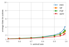
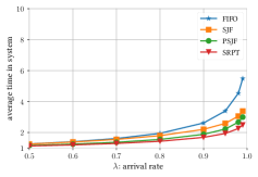
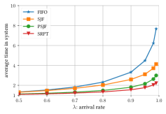
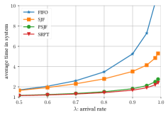
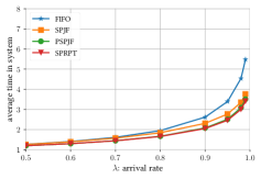
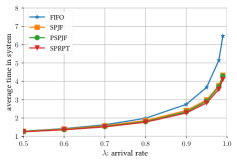
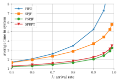
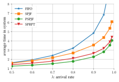
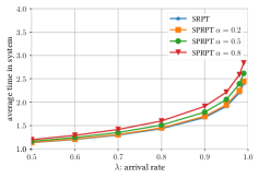
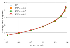
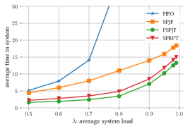
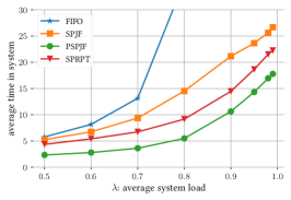
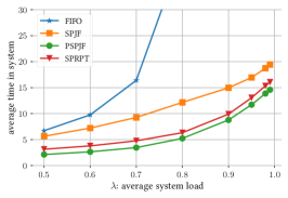
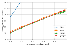
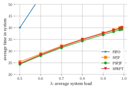
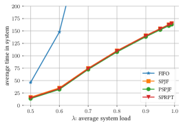
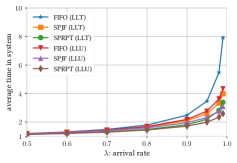
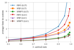
Figure 1(a) shows the results where the least loaded queue is chosen (ties broken randomly), while Figure 1(b) shows the results where the shortest queue is chosen, for exponential service times. Figures 1(c) and 1(d) present the results for the Weibull distributed service times. Generally, we see that the results from using the known service times to order jobs at the queue is very powerful; indeed, the gain from using SRPT appears larger than the gain from moving from shortest queue to least loaded, and similarly the gain from using SJF and PSJF is larger under high enough loads.

As the charts make it somewhat more difficult to see some important details, we present numerical results for exponentially distributed service times in Table I to mark some key points. While generally the benefits from using the service times to both choose the queue and order the queue are complementary, this is not always the case. We see that using least loaded rather than shortest queue when using PSJF can increase the average time in the system under suitably high load. (This also occurs with the Weibull distribution under sufficiently high loads.) We also see that using PSJF can give worse performance than using SJF; however, this does not happen with our experiments with the Weibull distribution, where the ability of preemption to help avoid waiting for long-running jobs appears to be more helpful. While it is known that PSJF can behave worse than SJF, these examples highlight that the interactions when using service time information in multiple choice systems must be treated carefully.

3.2 Choosing a Queue with Exact Information

Given the improvements possible using known service times in the supermarket model, we now consider methods for choosing a queue beyond the queue with the least load, in the setting without predictions. Given full information about the service times of jobs at each queue, a job could be placed so that it minimizes the additional waiting time. The additional waiting time when placing an arriving job is the sum of the remaining service times of all jobs in the queue that will remain ahead of the arriving job, summed with the product of the service time of the arriving job and the number of jobs it will be placed ahead of. Equivalently, we can consider the total waiting time for each queue before and after the arriving job would be placed (ignoring the possibility of future jobs), and place the item in the queue that leads to the smallest increase.

Alternatively, if control is not centralized, we might consider selfish jobs, that seek only to minimize their own waiting time when choosing a queue. In this case the arriving job will consider the sum of the remaining service times of all jobs that will be ahead of it for each available queue choice.

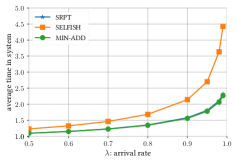
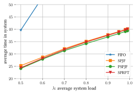
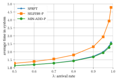
Our results, given in Figure 2, show that choosing a queue to minimize the additional waiting time in these situations does yield a small improvement over least loaded SRPT, as might be expected. Because the additional improvement is small, we expect in many systems it may not be worthwhile to implement this modification, even if expected waiting time is the primary performance metric. Our results also show that while selfish jobs have a significant negative effect, the overall average service time still remains smaller than the standard supermarket model when choosing the shorter of two FIFO queues.

4 Predicted Service Times

In many settings, it may be unreasonable to expect to obtain exact service times, but predicted service times may be available. Indeed, with advances in ML techniques, we expect that in many settings some type of prediction will be available. As noted in [22], in the context of scheduling within a single queue, one would expect that even weak predictors may be very useful, since ordering jobs correctly most of the time will produce significant gains. As we have seen, however, even without predictions the question of whether using load information for both choosing a queue and for ordering within a queue provides complementary gains is not always clear. Naturally, the same question will arise again when using predicted service times.

4.1 The Prediction Model

In what follows, we utilize a simple model used in [22], namely that there is a continuous joint distribution $g(x,y)$ for the actual service time $x$ and predicted service time $y$ .

With this model, there remains an issue of how to describe the predicted remaining service time. Suppose that the original predicted service time for a job is $y$ , but the actual service time is $x>y$ . If the amount of service is being tracked, and the service received has been $t$ , then as the remaining service time is $x-t$ , it is natural to use $y-t$ as the predicted remaining service time. Of course, at some point it becomes the case that $t>y$ , and the predicted remaining service time will be negative, which seems unsuitable.

We use $(y-t)^{+}=\max(y-t,0)$ as the predicted remaining service time. We recognize (as noted in [22]) that this is problematic; clearly the predicted remaining service time should be positive, and ideally would be a function $f(y,t)$ of the initial prediction and the time served thus far. However, determining the appropriate function would appear to require some knowledge of the joint distribution $g(x,y)$ ; our aim here is to explore simple, general approaches (such as choosing the shortest of two queues and using SRPT) that are agnostic to the underlying distribution $g$ . In many situations, it may be computationally undesirable to utilize knowledge of $g$ , or $g$ may be not known or changing over time. We therefore leave the question of how to optimize the estimate of the predicted remaining time to achieve the best performance in this context as future work.

We consider various models for predictions (some of which were used in [22]). The models are intended to be exemplary; they do not match a specific real-world setting, and indeed it would be difficult to consider the range of possible real-world predictions. Rather, they are meant to show generally that even moderately accurate predictions can yield strong performance, and to show that a variety of interesting behaviors can occur under this framework.

In one model, which we refer to as exponential predictions, a job with actual service time $x$ has a predicted service time that is exponentially distributed with mean $x$ . This model is not meant to accurately represent a specific situation, but is potentially useful for theoretical analysis in that the corresponding density equation $g(x,y)$ is easy to write down, has a non-zero probability for even very large prediction errors (note that the predicted service time will be any given constant factor larger than the true service time with constant probability), and it highlights how even noisy (and sometimes extremely incorrect) predictions can perform well. Also, exponential service times are a standard first consideration in queueing theory. In another model, which we refer to as $\alpha$ -predictions, a job with service time $x$ has a predicted service time that is uniform over $[(1-\alpha)x,(1+\alpha)x]$ , for a scale parameter $0\leq\alpha\leq 1$ . Again, this is a simple model that captures inaccurate estimates naturally. Finally, we introduce a model that we dub $(\alpha,\beta)$ -predictions, which makes use of the following notion of a reversal. For a service distribution with the cumulative distribution function $S(x)$ , the reversal of $x$ is $S^{-1}(1-S(x))$ . For example, if $x$ is the value that is at the 70th percentile of the distribution, the reversal is the value at the 30th percentile of the distribution. For an $(\alpha,\beta)$ -prediction, when the service time is $x$ , with probability $\beta$ we return the reversal of $x$ , and with all remaining probability the predicted service time is uniform over $[(1-\alpha)x,(1+\alpha)x]$ . We use this model to represent cases where severe mispredictions are possible, so that jobs with very large service times might be mistakenly predicted as having very small service times (and vice versa). We might expect such mispredictions could be potentially very problematic when scheduling jobs according to their predicted service times.

There remains the question of how to account for the predicted workload at a queue. We discuss several variations.

1.

Least Loaded Total: One could simply treat the predicted service times as actual service times, and track the total predicted service time remaining at a queue. That is, when a new job arrives at a queue, the predicted service time for the job is added to the total, and the total predicted service time reduces at a rate of one unit per unit time when a job is in the system (with a lower bound of 0); when the queue empties, the total predicted service time is reset to 0. An advantage of this approach is that in implementation the queue state can be represented by a single number. The disadvantage is that when a job’s predicted service time differs greatly from the real service time, this approach does not correspondingly update when that job completes.
2.

Least Loaded Updated: Here one updates the queue state both on a job arrival and a job completion; when a job completes, the predicted service time at the queue is recomputed as the sum of the predicted service times of the remaining jobs. With small additional complexity, the accuracy of the predicted work at the queue improves substantially.
3.

Shortest Queue: One can always simply use the number of jobs rather than the predicted service time to choose the queue.

We note Least Loaded Updated performs much better than Least Loaded Total, and focus on it for the rest of the paper. More on the comparison is given in Section A.2.

4.2 Scheduling with Predictions

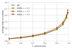
We begin as before by first considering the effect of the choice of scheduling procedure within a queue, by examining results for FIFO, shortest predicted job first (SPJF), preemptive shortest predicted job first (PSPJF), and shortest predicted remaining processing time (SPRPT) in various settings. Our figures consider the least loaded updated and shortest queue variations described above (as the least loaded total variation generally performs significantly worse, and so we do not generally consider this model, although for comparison purposes we present some results for it in the next subsection). We again consider exponential and Weibull distributed service times as previously described.

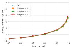
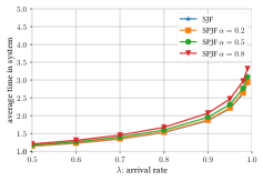
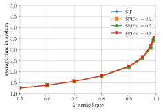
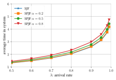
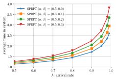
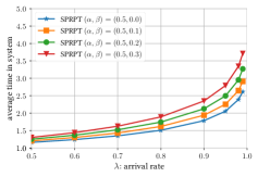
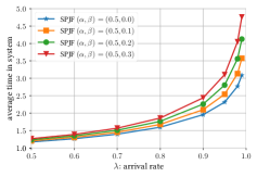
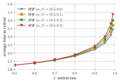
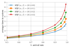
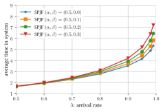
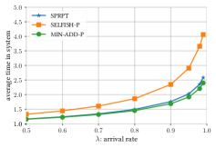
Our first results for exponential predictions, shown in Figure 3, already show two key points: predicted service times can work quite well, but there are also surprising and interesting behaviors. First, choosing the shortest queue generally performs quite similarly to choosing the least loaded according to the predicted service times of jobs in the queue; for this set of experiments, choosing the queue based on its predicted load still slightly outperforms using just the number of jobs, but we will see this is not the case in other settings. That is, when using strategies within the queue that utilize the predicted information, it can be worse to use the predicted load to choose the queue. Hence using predicted information for multiple subtasks (choosing a queue, and balancing within a queue) may not be beneficial and can even lead to worse performance than simply using the information for one of the subtasks. Second, PSPJF performs better than SPRPT on the Weibull distribution. On reflection, this seems reasonable from first principles; a long job that is incorrectly predicted to have a small remaining processing time can lead to increased waiting times for many jobs under SPRPT, but preempting based on the initial prediction of the job time ameliorates this effect.

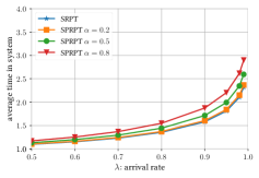
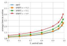
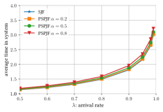
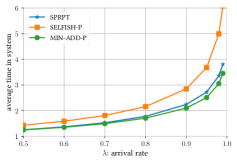
We now examine results in the setting of $\alpha$ -predictions. We first look at the case of SPRPT; results for other schemes have similar characteristics. We compare SRPT (no prediction) with SPRPT for $\alpha=0.2,0.5,$ , and $0.8$ , both using the least loaded update and shortest queue policies. The results appear in Figure 4.³³3We note that in some of our plots throughout this section, the lines for SRPT or SJF are hard to distinguish, as they are very close to other plotted results. The primary takeaway is that again using predictions offers what is arguably surprisingly little loss in performance, even at large values of $\alpha$ . Here, we find that least loaded does better than shortest queue for exponential service times, but for the more skewed Weibull distribution and $\alpha=0.8$ shortest queue can perform slightly better. With large errors and skewed service time distributions, using predictions both to choose a queue and within a queue can lead to over-using the predictions and worse performance.

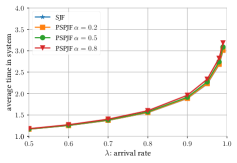
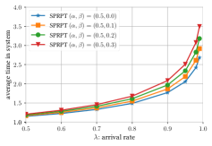
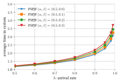
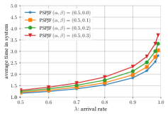
We also look at the case of PSPJF in Figure 5. Performance is somewhat worse than for SPRPT, and the effect of increasing $\alpha$ is smaller. Here, we find that joining the shortest queue generally does better than joining the least loaded queue. Overall the picture remains very similar.

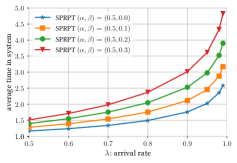
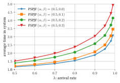
For completeness we also provide results using SPJF, which generally performs worse than SPRPT and PSPJF, in Figure 6. However, the effect on performance as $\alpha$ increases rises even more slowly with $\alpha$ . In these experiments, using least loaded always performed better than choosing the shortest queue.

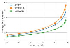
Finally, we consider the case of $(\alpha,\beta)$ -predictions. Here we present an example of $\alpha=0.5$ with $\beta=0.1,0.2$ , and $0.3$ , comparing also with the results from $\alpha$ -prediction when $\alpha$ = 0.5. Recall that in this setting with probability $\beta$ a job’s service time is replaced by its reversal in the cumulative distribution function, so that jobs with very large service times might be mistakenly predicted as having very small service times (and vice versa). The remaining jobs have predictions uniform over $[(1-\alpha)x,(1+\alpha)x]$ when the true service time is $x$ . The results for SPRPT are given in Figure 7, for PSPJF are given in Figure 8, and for SPJF are given in Figure 9. The primary takeaway is again that performance is quite robust to mispredictions. Even when $\beta=0.3$ , performance in all cases is significantly better than for standard choosing the shortest of two queues and using FIFO queueing without knowledge of service times. We also see now familiar trends. The effects of misprediction are more significant for the heavy-tailed service times, and when mispredictions are sufficiently frequent, it becomes better to choose a queue according to the shortest queue rather than according to the least loaded updated policy. Also, in some cases PSPJF can outperform SPRPT (compare, e.g., Figure 7(c) and Figure 8(c) with $\beta=0.2$ and $\lambda\leq 0.8$ ).

4.2.1 Fairness Issues

As the general problem of utilizing predictions for queue scheduling is relatively new, we have focused here on examining expected response time. We point out, however, that there are novel problems regarding questions such as fairness in the setting where predictions are used. For example, a standard notion of fairness involves considering job slowdown, i.e., the ratio $T(x)/x$ between a job $j$ ’s response time $T(x)$ and its service time $x$ , and the mean conditional slowdown $E[T(x)]/x$ [4, 32, 33]. Not surprisingly, we find that when using predictions, even when using scheduling methods based on SRPT, which is often fair or limited in its unfairness (see the discussion in [32]), the proposed variations using prediction have very poor fairness.

This occurs for multiple reasons. Most significantly, even very short jobs can be caught waiting for jobs with a remaining predicted service of zero. This leads to occasional large values of $T(x)/x$ for small jobs, skewing the fairness. Also, in cases where small jobs obtain large predictions, the value of $T(x)/x$ can again be high under high load.

The two problems suggest different solutions. In the first case, $T(x)$ is artificially high; this suggests strong fairness results require policies that do something beyond letting jobs with predicted remaining service time zero continue. Some addition of processor sharing, preemption, or modifying the prediction when the predicted remaining service time reaches zero should therefore improve fairness. In the second case, $x$ is small when the predicted time $y$ is large; this suggests that the responsibility of a given job’s slowdown is shared between the scheduler and the component responsible for service time prediction. To more accurately illustrate the interplay between those components, we speculate that alternative definitions of fairness, based on the prediction $y$ as well as the actual service time $x$ , should be considered.

We provide some preliminary results on fairness in Appendix B, and leave additional study for further work.

5 Real-World Traces

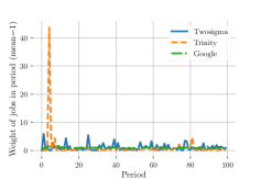
We now consider how the scheduling policies deal with real-world traces by Amvrosiadis et al. [2], who developed a system that predicts service time in large real-world clusters. The service time predictions are generated through a machine-learning system that focuses on detecting jobs that repeat on large compute clusters, using features such as user ID and job names in addition to information such as input size; further details are given by Tumanov et al. [29]. For each job, we have the submission time and its real and predicted runtime in seconds (for multi-task jobs, their service times were obtained by summing the service time (resp. predicted service time) of each individual task); we only take into account the jobs that completed successfully. For consistency with the synthetic traces, we normalize service time to obtain a mean of 1. We have three traces: Google (385,072 jobs), Trinity (18,872 jobs), and Twosigma (265,029 jobs). In Figure 10, we divide each trace in 100 periods, and plot the cumulative service time of jobs submitted in that period, normalized such that the mean value per period is 1. We have very different job submission patterns: most of the load for the Trinity dataset is concentrated around the beginning of the trace; the Twosigma dataset has lower load spikes along the whole trace; finally, the Google dataset has a relatively more uniform load pattern.⁴⁴4Amvrosiadis et al. discuss a fourth trace (Mustang). However, we have found that this case falls in the extreme service time skew and inaccuracy scenario where predicted size-based scheduling is ineffective we referred to in Section 2 [8, 22]. For this reason, we do not include results from that dataset in this paper.

To obtain an average system load of $\lambda$ while maintaining the original patterns of job submission times, we normalize job submission times by multiplying them by a constant factor such that the average interval between jobs is $1/q\lambda$ , where $q=100$ is the number of queues in the simulation. Since there is a degree of randomness due to the random choice of queues, we repeated the experiment 5 times for each settings, with negligible differences in the end results. Results shown here represent the average of the 5 runs.

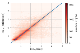
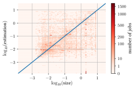
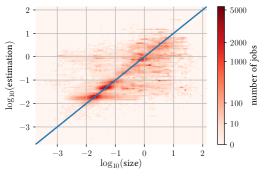
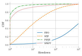
In Figure 11, we show heatmaps covering the joint distribution of job real and predicted service time. In what we believe is a common real-world pattern, the service time distribution is heavy tailed, with a few large jobs representing a large amount of the overall system load; service times are distributed along several orders of magnitude.

In Figure 12, we show results for the Google dataset. The variation of system load in time yields higher absolute numbers for the mean time in system compared to the synthetic datasets seen before; this phenomenon is stronger in the other datasets because they have larger load spikes, as seen in Figure 10. Similarly to some use cases for synthetic workloads seen before, we observe that also here shortest queue performs better than least loaded updated. Interestingly, the selfish strategy instead performs essentially as well as shortest queue, showing that in this scenario the “price of anarchy” (i.e., the performance cost due to letting each job’s owner selfishly choose their queue) is negligible. Perhaps surprisingly, the selfish strategy outperforms least loaded updated. The main difference between the two strategies is that the former ignores the load due to larger jobs; as a result, and at the price of worse performance for larger jobs, smaller jobs get served earlier. Since smaller jobs are the majority, the average response time is better with selfish queue selection. We further note that, unsurprisingly, the size-based scheduling policies largely outperform FIFO scheduling in this heavy-tailed workload, and—again confirming results for synthetic workloads—PSPJF is preferable to the other policies due to its better performance in the case that is most problematic for other policies, i.e., when large jobs are underestimated [9, 8].

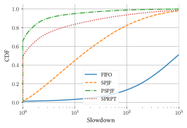
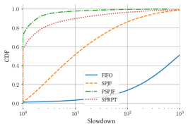
In the other two datasets (Figures 13 and 14) results are qualitatively similar, even though the larger load spikes further increase the average time spent in the system. The difference between FIFO and the other policies is even larger, while PSPJF remains the best-performing one. The difference between policies is smaller, compared to the large advantage due to choosing a policy based on predicted service time. We explain this phenomenon with the fact that, in these traces with large load spikes, most of the waiting time is spent in very long queues during these spikes. In such cases, size-based policies behave in a largely similar way, giving small jobs priority over large ones; this explains the large gaps between them and FIFO. The difference between them, i.e., how preemption is implemented, plays a comparatively small role. Conversely, in the more balanced Google dataset, most jobs spend their waiting time in shorter queues; in this case preemption can impact waiting time more frequently.

6 Conclusion

We have considered, primarily through simulation, the supermarket model in the setting where service times are predicted. As a starting point, however, we considered the baseline where service times are known. Our results show that in the “standard” supermarket model (exponential service times, Poisson arrivals) as well as more generally, even though the supermarket model provides tremendous gains over a single choice, there remains substantial further performance gains to be achieved when one makes use of known service times. In particular, a service-aware scheduling policy such as SRPT can yield significant performance gains under high loads. This raises natural theoretical questions, such as deriving equations for the supermarket model using least loaded server selection with shortest job first or shortest remaining processing time, which would extend the recent work of [12].

However, our more important direction is to introduce the idea of using predicted service times in this setting. Our simulation-based study allows us to evaluate this setting also on real-world traces, and suggests that the supermarket model maintains most of its power even when using predictions, as long as they are reasonably precise. We also find some interesting, potentially counterintuitive effects. For example, choosing queue by length rather than predicted load can be beneficial when predictions are also used within the queue, because when predictions are sufficiently inaccurate using them for both choosing a queue and scheduling within it can be detrimental. We view our results as showing the use of predicted service times in large-scale distributed systems can be quite promising in terms of improving performance.

A practical piece of advice we can give for implementation in concrete systems is using shortest queue selection and PSPJF. This policy is simple to understand and implement, and our results show it performs very well in a quite wide variety of cases, being outperformed by non size-based scheduling only in extreme cases where predictions are particularly non-informative. While SPRPT for example can be a better scheduling policy when predictions are quite accurate, PSJPF appears more robust. To evaluate the benefits of this policy and to possibly find better solutions for particular use cases, a further step can be replaying system traces in a simulator as done in this work.

Our work highlights many open practical questions on how to optimize these kinds of systems when using predictions, as well as many open theoretical questions regarding how to analyze these kinds of systems. For example, suitable mechanisms for managing jobs that exceed their predicted service time offer further potential for important improvements. Perhaps most interesting is developing appropriate theories of fairness when using predictions. A short job predicted to have a long service time may face long delays before service; how to achieve a suitable notion of fairness when using predictions clearly merits further study.

Acknowledgment

The authors would like to thank Amvrosiadis et al. [2] for sharing their predictions datasets.

References

[1] Reza Aghajani, Xingjie Li, and Kavita Ramanan. Mean-field dynamics of load-balancing networks with general service distributions. arXiv preprint arXiv:1512.05056, 2015.
[2] George Amvrosiadis, Jun Woo Park, Gregory R. Ganger, Garth A. Gibson, Elisabeth Baseman, and Nathan DeBardeleben. On the diversity of cluster workloads and its impact on research results. In Proceedings of the 2018 USENIX Annual Technical Conference, 2018.
[3] Yossi Azar, Andrei Z. Broder, Anna R. Karlin, and Eli Upfal. Balanced allocations. SIAM J. Comput., 29(1):180–200, 1999.
[4] Nikhil Bansal and Mor Harchol-Balter. Analysis of SRPT scheduling: investigating unfairness. In Proceedings of the Joint International Conference on Measurements and Modeling of Computer Systems, pp. 279-290, 2001.
[5] René Bekker, Sem C Borst, Onno J Boxma, and Offer Kella. Queues with workload-dependent arrival and service rates. Queueing Systems, 46(3-4):537–556, 2004.
[6] Maury Bramson, Yi Lu, and Balaji Prabhakar. Randomized load balancing with general service time distributions. In ACM SIGMETRICS Performance Evaluation Review, volume 38, pages 275–286, 2010.
[7] Maury Bramson, Yi Lu, and Balaji Prabhakar. Asymptotic independence of queues under randomized load balancing. Queueing Systems, 71(3):247–292, 2012.
[8] Matteo Dell’Amico. Scheduling With Inexact Job Sizes: The Merits of Shortest Processing Time First. arXiv preprint arXiv:1907.04824, 2019.
[9] Matteo Dell’Amico, Damiano Carra, and Pietro Michiardi. PSBS: Practical size-based scheduling. IEEE Transactions on Computers, 65(7):2199-2212, 2015.
[10] Mor Harchol-Balter. Task assignment with unknown duration. J. ACM, 49(2):260–288, 2002.
[11] Mor Harchol-Balter. Performance modeling and design of computer systems: queueing theory in action. Cambridge University Press, 2013.
[12] Tim Hellemans and Benny Van Houdt. On the power-of- $d$ -choices with least loaded server selection. POMACS, 2(2):27:1–27:22, 2018.
[13] Tim Hellemans, Tejas Bodas, and Benny Van Houdt. Performance analysis of workload dependent load balancing policies. POMACS, 3(2):35:1–35:35, 2019.
[14] Chen-Yu Hsu, Piotr Indyk, Dina Katabi, and Ali Vakilian. Learning-based frequency estimation algorithms. International Conference on Learning Representations, 2019.
[15] Richard M. Karp, Michael Luby, and Friedhelm Meyer auf der Heide. Efficient PRAM simulation on a distributed memory machine. Algorithmica, 16(4/5):517–542, 1996.
[16] Tim Kraska, Alex Beutel, Ed H Chi, Jeffrey Dean, and Neoklis Polyzotis. The case for learned index structures. In Proceedings of the 2018 International Conference on Management of Data, pages 489–504. ACM, 2018.
[17] Thodoris Lykouris and Sergei Vassilvitskii. Competitive caching with machine learned advice. In Proceedings of the 35th International Conference on Machine Learning, ICML 2018, volume 80 of JMLR Workshop and Conference Proceedings, pages 3302–3311. JMLR.org.
[18] Raymond Marie. Calculating equilibrium probabilities for $\lambda$ (n)/c k/1/n queues. ACM Sigmetrics Performance Evaluation Review, 9(2):117–125, 1980.
[19] Michael Mitzenmacher. Studying balanced allocations with differential equations. Combinatorics, Probability & Computing, 8(5):473–482, 1999.
[20] Michael Mitzenmacher. How useful is old information? IEEE Trans. Parallel Distrib. Syst., 11(1):6–20, 2000.
[21] Michael Mitzenmacher. The power of two choices in randomized load balancing. IEEE Trans. Parallel Distrib. Syst., 12(10):1094–1104, 2001.
[22] Michael Mitzenmacher. Scheduling with predictions and the price of misprediction. arXiv preprint arXiv:1902.00732, 2019.
[23] Michael Mitzenmacher. A model for learned Bloom filters and optimizing by sandwiching. In Advances in Neural Information Processing Systems, pages 462–471, 2018.
[24] Michael Mitzenmacher and Eli Upfal. Probability and computing - randomized algorithms and probabilistic analysis. Cambridge University Press, 2005.
[25] Michael Mitzenmacher and Berthöld Vöcking. The asymptotics of selecting the shortest of two, improved. In Proceedings of the 37th Annual Allerton Conference on Communication, Control, and Computing, 1999.
[26] Manish Purohit, Zoya Svitkina, and Ravi Kumar. Improving online algorithms via ML predictions. In Advances in Neural Information Processing Systems, pages 9684–9693, 2018.
[27] Ziv Scully and Mor Harchol-Balter. SOAP bubbles: robust scheduling under adversarial noise. In Proceedings of the 56th Annual Allerton Conference on Communication, Control, and Computing, 2018.
[28] Ziv Scully, Mor Harchol-Balter and Allen Scheller-Wolf. SOAP: One Clean Analysis of All Age-Based Scheduling Policies. In Proceedings of the ACM on Measurement and Analysis of Computing Systems, 2018.
[29] Alexey Tumanov, Angela Jiang, Jun Woo Park, Michael A. Kozuch, Gregory R. Ganger. JamaisVu: Robust Scheduling with Auto-Estimated Job Runtimes. Tech. Rep. CMU-PDL-16-104, Carnegie Mellon University, September 2016.
[30] Berthold Vöcking. How asymmetry helps load balancing. Journal of the ACM, 50:4, 568-589, 2003.
[31] Nikita Dmitrievna Vvedenskaya, Roland L’vovich Dobrushin, and Fridrikh Izrailevich Karpelevich. Queueing system with selection of the shortest of two queues: An asymptotic approach. Problemy Peredachi Informatsii, 32(1):20–34, 1996.
[32] Adam Wierman. Fairness and scheduling in single server queues. Surveys in Operations Research and Management Science, 16(1), pp. 39-48, 2011.
[33] Adam Wierman and Mor Harchol-Balter. Classifying scheduling policies with respect to unfairness in an M/GI/1. In Proceedings of the International Conference on Measurements and Modeling of Computer Systems, pp. 238-249, 2003.
[34] Adam Wierman and Misja Nuyens. Scheduling despite inexact job-size information. Performance Evaluation Review, 36(1):25-36, 2008.

Appendix A Additional Results

A.1 Developing Equations for Limiting Behavior

Previous work has shown that, in the limiting supermarket model where the number of queues goes to infinity, individual queues can be treated as independent, both when the choosing shortest queue and when choosing the least loaded [7]. This connection plays a key role in the analysis of the supermarket model when choosing the least loaded queue with FIFO scheduling in [12], which yields the stationary distribution for the queue load for individual queues in the limit as $n$ goes to infinity. (See also [13] on this issue; this is sometimes referred to as cavity process analysis.) We can conclude that in equilibrium, at each queue considered in isolation, the least loaded variant of the supermarket model has a load-dependent arrival process, given by a Poisson process of rate $\lambda(x)$ when the queue has service load $x$ . (See, for example, [5, 18] for more on queues with load-dependent arrival processes; note here the arrival rate depends on the workload, not the total number of jobs in the queue.) The least loaded variant of the supermarket model when using other scheduling schemes, such as SJF, PSJF, and SRPT, would similarly have the same load-dependent arrival process, as in equilibrium the workload distribution would be the same regardless of the scheduling scheme. Hence we could develop formulae for quantities such as the expected time in system in equilibrium in the supermarket model using the least loaded queue and SRPT, if we can develop an analysis of a single queue using SRPT with a load-dependent arrival process (and similarly for other scheduling schemes). We are not aware of any such analysis in the literature, and we know of no current technique that provides such an analysis; this is a natural and tantalizing open question.

We note that the supermarket model when jobs choose the shortest queue also, as far as we know, has not been analyzed for SJF, PSJF, and SRPT. Here the arrival process at a queue in equilibrium can be given by a Poisson process of rate $\lambda(n)$ when the queue has $n$ jobs waiting. Again, if we can develop an analysis of a single queue using SRPT with a queue-length-dependent arrival process, we can use this to analyze the supermarket model using SRPT (and similarly for other scheduling schemes). Again, we are not aware of any such analysis in the literature, and this is a natural and tantalizing open question.

A.2 Choosing a Queue with Predictions

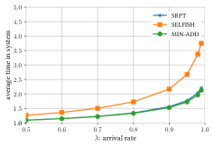
As before, we consider methods for choosing a queue beyond the queue with the (predicted) least load. We consider placing a job so that it minimizes the additional predicted waiting time, based on the predicted waiting times for all jobs. Alternatively, if control is not centralized, we might consider selfish jobs, that seek only to minimize their own predicted waiting time when choosing a queue.

Our results, in Figure 15, focus on two representative examples: $\alpha$ -predictions with $\alpha=0.5$ , and $(\alpha,\beta)$ -predictions with $\alpha=0.5,\beta=0.2$ . Again, choosing a queue to minimize the additional predicted waiting time in these situations does yield a small improvement over least loaded update with SPRPT, and selfish jobs have a significant negative effect.

Finally, as discussed earlier we note that there is a significant difference between Least Loaded Updated and Least Loaded Total policies. Up to this point, we have used “least loaded” to refer to Least Loaded Updated, where the predicted service time at the queue is recomputed after each departure and arrival. In contrast, Least Loaded Total tracks a single predicted service time for the queue that is updated on arrival but not at departure (unless a queue empties, in which case the service is reset to 0). While theoretically appealing (as it reduces the state space for the system), Least Loaded Total generally performs significantly worse than Least Loaded Updated. Figure 16 below provides a representative example, in the setting of $\alpha$ -predictions when $\alpha=0.5$ . We see FIFO, in particular, does quite poorly under Least Loaded Total, and in all cases, the gap in performance notably increases with the load. Our other experiments show that the gap in performance also increases significantly as the predictions become more inaccurate; with exponential predictions, $\alpha$ -predictions with higher $\alpha$ , or $(\alpha,\beta)$ -predictions with $\alpha=0.5$ and $\beta>0$ , our simulations show even larger gains from using Least Loaded Updated. While it may be useful to consider Least Loaded Total as an approach toward obtaining theoretical results, it does not appear to be the result we wish to aim for.

Appendix B Fairness

As described in Section 4.2.1, fairness is often defined in terms of making jobs spend an amount of time in the system that is roughly proportional to their service time [32]; this is captured by the slowdown concept, where a job’s slowdown is its resident time divided by its service time. Here, we will show results relative to the real-world datasets of Section 5 where the average system load is set to $\lambda=0.9$ .

B.1 Slowdown Distribution

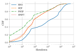
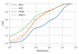
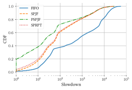
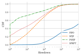
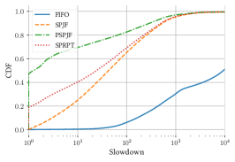
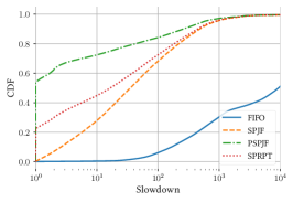
A first definition of fairness can be having predictable slowdowns: for example, minimizing the variance of the per-job slowdowns, or a given value for the $x$ -th percentile. To facilitate these evaluations, in Figures 17, 18 and 19 we show the empirical cumulative distribution functions (CDFs) of the slowdown values observed in our experiments.

Because system load changes over time, slowdown distributions are unequal in essentially all cases that we observe–in particular for Trinity, due to the large load the system experiences around the beginning of the trace. The overall pattern we see here, however, is that the slowdown distribution becomes less unequal with policies that perform better; PSPJF, which is the policy that performs best in terms of mean time in system, also has the least variability in terms of slowdown. We explain this intuitively with the fact that extreme slowdown values are caused by “clogged” queues: by optimizing mean time in system, extreme slowdown cases are also minimized.

B.2 Mean Conditional Slowdown

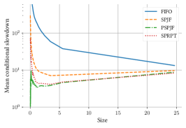
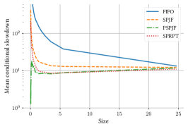
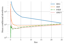
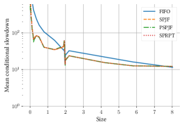
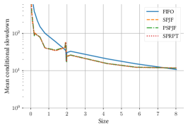
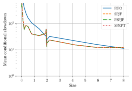
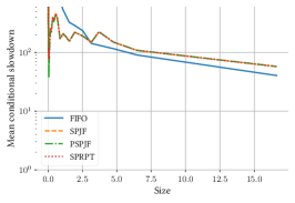
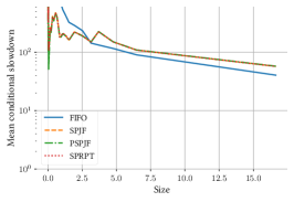
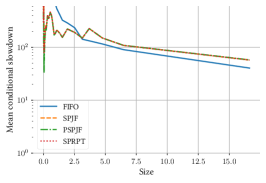
A second definition of fairness involves mean conditional slowdown, that is, the expected value of slowdown for job having a given service time: for a job having service time $x$ , the mean conditional slowdown is $E[T(x)]/x$ , where $T(x)$ is the time in system for jobs having service time $x$ [4, 32, 33]. To evaluate it empirically in our experiments, we follow the approach of Dell’Amico et al. [9], bin jobs by service time in 50 bins having the same amount of jobs each, and plot the average service time and slowdown of each bin in Figures 20, 21 and 22, respectively on the X and Y axis.

Once again, and confirming esisting research [32, 9], we observe that best-performing policies empirically result in better fairness. While one may imagine that size-based policies that give priority to smaller jobs would penalize large ones compared to a policy like FIFO, this is only true to some extent: for Google (Figure 20) size-based policies appeared to always be preferable also for larger jobs; in Trinity (21) only the very largest jobs are penalized; only in the Twosigma dataset large jobs have sensibly lower mean conditional slowdown when size-based policies are used.

In Figure 21, we notice a discontinuity for jobs of service time 2. This can be explained by Figure 11, which shows that for the Trinity dataset there is a set of jobs having service time 2 whose service time is systematically underestimated: this explains the drop in mean conditional slowdown.

For Twosigma (Figure 22), the results for all the size-based scheduling algorithms look superimposed. We explain this, once again, with the data from Figure 11, showing that service time estimations tend to be clustered around some well-separated values; hence, the details of the scheduling algorithm only have limited impact, since in most cases they will all schedule the job with the smallest estimated service time.

The Supermarket Model with Known and Predicted Service Times