Optimal approximation for unconstrained
non-submodular minimization

Abstract

Submodular function minimization is well studied, and existing algorithms solve it exactly or up to arbitrary accuracy. However, in many applications, such as structured sparse learning or batch Bayesian optimization, the objective function is not exactly submodular, but close. In this case, no theoretical guarantees exist. Indeed, submodular minimization algorithms rely on intricate connections between submodularity and convexity. We show how these relations can be extended to obtain approximation guarantees for minimizing non-submodular functions, characterized by how close the function is to submodular. We also extend this result to noisy function evaluations. Our approximation results are the first for minimizing non-submodular functions, and are optimal, as established by our matching lower bound.

1 Introduction

Many machine learning problems can be formulated as minimizing a set function $H$. This problem is in general NP-hard, and can only be solved efficiently with additional structure. One especially popular example of such structure is that $H$ is submodular, i.e., it satisfies the diminishing returns (DR) property: $H(A\cup\{i\})-H(A)\geq H(B\cup\{i\})-H(B)$, for all $A\subseteq B,i\in V\setminus B$. Several existing algorithms minimize a submodular $H$ in polynomial time, exactly or within arbitrary accuracy. Submodularity is a natural model for a variety of applications, such as image segmentation (Boykov & Kolmogorov, 2004), data selection (Lin & Bilmes, 2010), or clustering (Narasimhan et al., 2006). But, in many other settings, such as structured sparse learning, Bayesian optimization, and column subset selection, the objective function is not exactly submodular. Instead, it satisfies a weaker version of the diminishing returns property. An important class of such functions are $\alpha$-weakly DR-submodular functions, introduced in (Lehmann et al., 2006). The parameter $\alpha$ quantifies how close the function is to being submodular (see Section 2 for a precise definition). Furthermore, in many cases, only noisy evaluations of the objective are available. Hence, we ask: Do submodular minimization algorithms extend to such non-submodular noisy functions?

Non-submodular maximization, under various notions of approximate submodularity, has recently received a lot of attention (Das & Kempe, 2011; Elenberg et al., 2018; Sakaue, 2019; Bian et al., 2017; Chen et al., 2017; Gatmiry & Gomez-Rodriguez, 2019; Harshaw et al., 2019; Kuhnle et al., 2018; Horel & Singer, 2016; Hassidim & Singer, 2018). In contrast, only few studies consider minimization of non-submodular set functions. Recent works have studied the problem of minimizing the ratio of two set functions, where one (Bai et al., 2016; Qian et al., 2017a) or both (Wang et al., 2019) are non-submodular. The ratio problem is related to constrained minimization, which does not admit a constant factor approximation even in the submodular case (Svitkina & Fleischer, 2011). If the objective is approximately modular, i.e., it has bounded curvature, algorithmic techniques related to those for submodular maximization achieve optimal approximations for constrained minimization (Sviridenko et al., 2017; Iyer et al., 2013). Algorithms for minimizing the difference of two submodular functions were proposed in (Iyer & Bilmes, 2012; Kawahara et al., 2015), but no approximation guarantees were provided.

In this paper, we study the unconstrained non-submodular minimization problem

$$\min\nolimits_{S\subseteq V}\;H(S):=F(S)-G(S),$$ (1)

where $F$ and $G$ are monotone (i.e., non-decreasing or non-increasing) functions, $F$ is $\alpha$-weakly DR-submodular, and $G$ is $\beta$-weakly DR-supermodular, i.e., $-G$ is ${\beta^{-1}}$-weakly DR-submodular. The definitions of weak DR-sub-/supermodularity only hold for monotone functions, and thus do not directly apply to $H$. We show that, perhaps surprisingly, any set function $H$ can be decomposed into functions $F$ and $G$ that satisfy these assumptions, albeit with properties leading to weaker approximations when the function is far from being submodular.

A key strategy for minimizing submodular functions exploits a tractable tight convex relaxation that enables the use of convex optimization algorithms. But, this relies on the equivalence between the convex closure of a submodular function and the polynomial-time computable Lovász extension. In general, the convex closure of a set function is NP-hard to compute, and the Lovász extension is convex if and only if the set function is submodular. Thus, the optimization delicately relies on submodularity; generally, a tractable tight convex relaxation is impossible. Yet, in this paper, we show that for approximately submodular functions, the Lovász extension can be approximately minimized using a projected subgradient method (PGM). In fact, this strategy is guaranteed to obtain an approximate solution to Problem (1). This insight broadly expands the scope of submodular minimization techniques. In short, our main contributions are:

• the first approximation guarantee for unconstrained non-submodular minimization characterized by closeness to submodularity: PGM achieves a tight approximation of $H(S)\leq{F(S^{*})}/\alpha-\beta G(S^{*})+\epsilon$;

• an extension of this result to the case where only a noisy oracle of $H$ is accessible;

• a hardness result showing that improving on this approximation guarantee would require exponentially many queries in the value oracle model;

• applications to structured sparse learning and variance reduction in batch Bayesian optimization, implying the first approximation guarantees for these problems;

• experiments demonstrating the robustness of classical submodular minimization algorithms against noise and non-submodularity, reflecting our theoretical results.

2 Preliminaries

We begin by introducing our notation, the definitions of weak DR-submodularity/supermodularity, and by reviewing some facts about classical submodular minimization.

Notation

Let $V=\{1,\cdots,d\}$ be the ground set. Given a set function $F:2^{V}\to\mathbb{R}$, we denote the marginal gain of adding an element $i$ to a set $A$ by $F(i|A)=F(A\cup\{i\})-F(A)$. Given a vector $\boldsymbol{x}\in\mathbb{R}^{d}$, $x_{i}$ is its $i$-th entry and $\mathrm{supp}(\boldsymbol{x})=\{i\in V|x_{i}\not=0\}$ is its support set; $\boldsymbol{x}$ also defines a modular set function as $\boldsymbol{x}(A)=\sum_{i\in A}x_{i}$.

Set function classes

The function $F$ is normalized if $F(\emptyset)=0$, and non-decreasing (non-increasing) if $F(A)\leq F(B)$ ($F(A)\geq F(B)$) for all $A\subseteq B$. $F$ is submodular if it has diminishing marginal gains: $F(i|A)\geq F(i|B)$ for all $A\subseteq B$, $i\in V\setminus B$, modular if the inequality holds as an equality, and supermodular if $F(i|A)\leq F(i|B)$. Relaxing these inequalities leads to the notions of weak DR-submodularity/supermodularity introduced in (Lehmann et al., 2006) and (Bian et al., 2017), respectively.

Definition 1 (Weak DR-sub/supermodularity).

A set function $F$ is $\alpha$-weakly DR-submodular, with $\alpha>0$, if

$$F(i|A)\geq\alpha F(i|B),\text{ for all $A\subseteq B,i\in V\setminus B$}.$$

Similarly, $F$ is $\beta$-weakly DR-supermodular, with $\beta>0$, if

$$F(i|B)\geq\beta F(i|A),\text{ for all $A\subseteq B,i\in V\setminus B$}.$$

We say that $F$ is $(\alpha,\beta)$-weakly DR-modular if it satisfies both properties.

If $F$ is non-decreasing, then $\alpha,\beta\in(0,1]$, and if it is non-increasing, then $\alpha,\beta\geq 1$. $F$ is submodular (supermodular) iff $\alpha=1$ ($\beta=1$) and modular iff both $\alpha=\beta=1$.
The parameters $1\!-\!\alpha$ and $1\!-\!\beta$ are referred to as generalized inverse curvature (Bogunovic et al., 2018) and generalized curvature (Bian et al., 2017), respectively. They extend the notions of inverse curvature and curvature (Conforti & Cornuéjols, 1984) commonly defined for supermodular and submodular functions. These notions are also related to weakly sub-/supermodular functions (Das & Kempe, 2011; Bogunovic et al., 2018). Namely, the classes of weakly DR-sub-/super-/modular functions are respective subsets of the classes of weakly sub-/super-/modular functions (El Halabi et al., 2018, Prop. 8), (Bogunovic et al., 2018, Prop. 1), as illustrated in Figure 1. For a survey of other notions of approximate submodularity, we refer the reader to (Bian et al., 2017, Sect. 6).

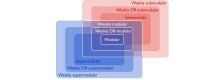
Figure 1: Classes of set functions

Submodular minimization

Minimizing a submodular set function $F$ is equivalent to minimizing a non-smooth convex function that is given by a continuous extension of $F$, i.e., a continuous interpolation of $F$ on the full hypercube $[0,1]^{d}$. This extension, called the Lovász extension (Lovász, 1983), is convex if and only if $F$ is submodular.

Definition 2 (Lovász extension).

Given any normalized set function $F$, its Lovász extension $f_{L}:\mathbb{R}^{d}\to\mathbb{R}$ is defined as

$$f_{L}(\boldsymbol{s})=\sum_{k=1}^{d}s_{j_{k}}F(j_{k}|S_{k-1}),$$

where $s_{j_{1}}\geq\cdots\geq s_{j_{d}}$ are the sorted entries of $\boldsymbol{s}$ in decreasing order, and $S_{k}=\{j_{1},\cdots,j_{k}\}$.

Minimizing $f_{L}$ is equivalent to minimizing $F$ . Moreover, when $F$ is submodular, a subgradient $\boldsymbol{\kappa}$ of $f_{L}$ at any $\boldsymbol{s}\in\mathbb{R}^{d}$ can be computed efficiently by sorting the entries of $\boldsymbol{s}$ in decreasing order and taking $\kappa_{j_{k}}=F(j_{k}|S_{k-1})$ for all $k\in V$ (Edmonds, 2003). This relation between submodularity and convexity allows for generic convex optimization algorithms to be used for minimizing $F$. However, it has been unclear how these relations are affected if the function is only approximately submodular. In this paper, we give an answer to this question.

3 Approximately submodular minimization

We consider set functions $H:2^{V}\to\mathbb{R}$ of the form $H(S)=F(S)-G(S)$, where $F$ is $\alpha$-weakly DR-submodular, $G$ is $\beta$-weakly DR-supermodular, and both $F$ and $G$ are normalized non-decreasing functions. We later extend our results to non-increasing functions. We assume a value oracle access to $H$; i.e., there is an oracle that, given a set $S\subseteq V$, returns the value $H(S)$. Note that $H$ itself is in general not weakly DR-submodular. Interestingly, any set function can be decomposed in this form.

Proposition 1.

Given a set function $H$, and $\alpha,\beta\in(0,1]$ such that $\alpha\beta<1$, there exists a non-decreasing $\alpha$-weakly DR-submodular function $F$, and a non-decreasing $(\alpha,\beta)$-weakly DR-modular function $G$, such that $H(S)=F(S)-G(S)$ for all $S\subseteq V$.

Proof sketch.

This decomposition builds on the decomposition of $H$ into the difference of two non-decreasing submodular functions (Iyer & Bilmes, 2012). We start by choosing any function $G^{\prime}$ which is non-decreasing $(\alpha,\beta)$-weakly DR-modular, and is strictly $\alpha$-weakly DR-submodular, i.e., $\epsilon_{G^{\prime}}=\min_{i\in V,A\subset B\subseteq V\setminus i}G^{\prime}(i|A)-\alpha G^{\prime}(i|B)>0$. It is not possible to choose $G^{\prime}$ such that $\alpha=\beta=1$ (this would imply $G^{\prime}(i|B)\geq G^{\prime}(i|A)>G^{\prime}(i|B)$). We then construct $F$ and $G$ based on $G^{\prime}$.
Let $\epsilon_{H}=\min_{i\in V,A\subseteq B\subseteq V\setminus i}H(i|A)-\alpha H(i|B)<0$ be the violation of $\alpha$-weak DR-submodularity of $H$; we may use a lower bound $\epsilon^{\prime}_{H}\leq\epsilon_{H}$. We define $F^{\prime}(S)=H(S)+\tfrac{|\epsilon^{\prime}_{H}|}{\epsilon_{G^{\prime}}}G^{\prime}(S)$. $F^{\prime}$ is not necessarily non-decreasing. To correct for that, let $V^{-}=\{i:F^{\prime}(i|V\setminus i)<0\}$ and define $F(S)=F^{\prime}(S)-\sum_{i\in S\cap V-}F^{\prime}(i|V\setminus i)$. We can show that $F$ is non-decreasing $\alpha$-weakly DR-submodular. We also define $G(S)=\tfrac{|\epsilon^{\prime}_{H}|}{\epsilon_{G^{\prime}}}G^{\prime}(S)-\sum_{i\in S\cap V-}F^{\prime}(i|V\setminus i)$, then $G$ is non-decreasing $(\alpha,\beta)$-weakly DR-modular, and $H(S)=F(S)-G(S)$. ∎

Proposition 1 generalizes the result of (Cunningham, 1983, Theorem 18) showing that any submodular function can be decomposed into the difference of a non-decreasing submodular function and a non-decreasing modular function. When $H$ is submodular, the decomposition in Proposition 1 recovers the one from (Cunningham, 1983), by simply choosing $\alpha=\beta=1$. The resulting violation of submodularity is $\epsilon_{H}=0$, and $G^{\prime}$ is not needed.

Computing such a decomposition is not required to run PGM for minimization; it is only needed to evaluate the corresponding approximation guarantee. The construction in the above proof uses the maximum violation $\epsilon_{H}$ of $\alpha$-weak DR-submodularity of $H$, which is NP-hard in general. However, when $\epsilon_{H}$ or a lower bound of it is known, $F$ and $G$ can be obtained in polynomial time, for a suitable choice of $G^{\prime}$. Proposition 2 provides a valid choice of $G^{\prime}$ for $\alpha=1$. Any modular function can be used for $\alpha<1$.

Proposition 2.

Given $\beta\in(0,1)$, let $G^{\prime}(S)=g(|S|)$ where $g(x)=\tfrac{1}{2}ax^{2}+(1-\tfrac{1}{2}a)x$ with $a=\tfrac{\beta-1}{d-1}$. Then $G^{\prime}$ is non-decreasing $(1,\beta)$-weakly DR-modular, and is strictly submodular, with $\epsilon_{G^{\prime}}=\min_{i\in V,A\subset B\subseteq V\setminus i}G^{\prime}(i|A)-G^{\prime}(i|B)=-a>0$.

The lower bound on $\epsilon_{H}$ and the choice of $\alpha,\beta$ and $G^{\prime}$ will affect the approximation guarantee on $H$, as we clarify later. When $H$ is far from being submodular, it may not be possible to choose $G^{\prime}$ to obtain a non-trivial guarantee. However, many important non-submodular functions do admit a decomposition which leads to non-trivial bounds. We call such functions approximately submodular, and provide some examples in Section 4.

In what follows, we establish a connection between approximate submodularity and approximate convexity, which allows us to derive a tight approximation guarantee for PGM on Problem (1). All omitted proofs are in the Supplement.

3.1 Convex relaxation

When $H$ is not submodular, the connections between its Lovász extension and tight convex relaxation for exact minimization, outlined in Section 2, break down. However, Problem (1) can still be converted to a non-smooth convex optimization problem, via a different convex extension. Given a set function $H$, its convex closure $h^{-}$ is the point-wise largest convex function from $[0,1]^{d}$ to $\mathbb{R}$ that always lower bounds $H$. Intuitively, $h^{-}$ is the tightest convex extension of $H$ on $[0,1]^{d}$. The following equivalence holds (Dughmi, 2009, Prop. 3.23):

$$\min_{S\subseteq V}H(S)=\min_{\boldsymbol{s}\in[0,1]^{d}}h^{-}(\boldsymbol{s}).$$ (2)

Unfortunately, evaluating and optimizing $h^{-}$ for a general set function is NP-hard (Vondrák, 2007). The key property that makes Problem (2) efficient to solve when $H$ is submodular is that its convex closure then coincides with its tractable Lovász extension, i.e., $h^{-}=h_{L}$. This equivalence no longer holds if $H$ is only approximately submodular. But, in this case, a weaker key property holds: Lemma 1 shows that the Lovász extension approximates the convex closure $h^{-}$, and that the same vectors that served as its subgradients in the submodular case can serve as approximate subgradients to $h^{-}$.

Lemma 1.

Given a vector $\boldsymbol{s}\in[0,1]^{d}$ such that $s_{j_{1}}\geq\cdots\geq s_{j_{d}}$, we define $\boldsymbol{\kappa}$ such that $\kappa_{j_{k}}=H(j_{k}|S_{k-1})$ where $S_{k}=\{j_{1},\cdots,j_{k}\}$. Then, $h_{L}(\boldsymbol{s})=\boldsymbol{\kappa}^{\top}\boldsymbol{s}\geq h^{-}(\boldsymbol{s})$, and

$$\boldsymbol{\kappa}(A) \leq\tfrac{1}{\alpha}F(A)-\beta G(A)\text{ for all }A\subseteq V,$$

$$\boldsymbol{\kappa}^{\top}\boldsymbol{s}^{\prime} \leq\tfrac{1}{\alpha}f^{-}(\boldsymbol{s}^{\prime})+\beta(-g)^{-}(\boldsymbol{s}^{\prime})\text{ for all }\boldsymbol{s}^{\prime}\in[0,1]^{d}.$$

To prove Lemma 1, we use a specific formulation of the convex closure $h^{-}$ (El Halabi, 2018, Def. 20):

$$h^{-}(\boldsymbol{s})=\max_{\boldsymbol{\kappa}\in\mathbb{R}^{d},\rho\in\mathbb{R}}\{\boldsymbol{\kappa}^{\top}\boldsymbol{s}+\rho:\boldsymbol{\kappa}(A)+\rho\leq H(A),\forall A\subseteq V\},$$

and build on the proof of Edmonds’ greedy algorithm (Edmonds, 2003). We can view the vector $\boldsymbol{\kappa}$ in Lemma 1 as an approximate subgradient of $h^{-}$ at $\boldsymbol{s}$ in the following sense:

$$\tfrac{1}{\alpha}f^{-}(\boldsymbol{s}^{\prime})+\beta(-g)^{-}(\boldsymbol{s}^{\prime})\geq h^{-}(\boldsymbol{s})+\langle\boldsymbol{\kappa},\boldsymbol{s}^{\prime}-\boldsymbol{s}\rangle,\forall\boldsymbol{s}^{\prime}\in[0,1]^{d}.$$

Lemma 1 also implies that the Lovász extension $h_{L}$ approximates the convex closure $h^{-}$ in the following sense:

$$h^{-}(\boldsymbol{s})\leq h_{L}(\boldsymbol{s})\leq\tfrac{1}{\alpha}f^{-}(\boldsymbol{s})+\beta(-g)^{-}(\boldsymbol{s}),\forall\boldsymbol{s}\in[0,1]^{d}.$$

We can thus say that $h_{L}$ is approximately convex in this case. This key insight allows us to approximately minimize $h^{-}$ via convex optimization algorithms.

3.2 Algorithm and approximation guarantees

Equipped with the approximate subgradients of $h^{-}$, we can now apply an approximate projected subgradient method (PGM). Starting from an arbitrary $\boldsymbol{s}^{1}\in[0,1]^{d}$, PGM iteratively updates $\boldsymbol{s}^{t+1}=\Pi_{[0,1]^{d}}(\boldsymbol{s}^{t}-\eta\boldsymbol{\kappa}^{t})$, where $\boldsymbol{\kappa}^{t}$ is the approximate subgradient at $\boldsymbol{s}^{t}$ from Lemma 1, and $\Pi_{[0,1]^{d}}$ is the projection onto $[0,1]^{d}$. We set the step size to $\eta=\tfrac{R}{L\sqrt{T}}$, where $L=F(V)+G(V)$ is the Lipschitz constant, i.e., $\|\boldsymbol{\kappa}^{t}\|_{2}\leq L$ for all $t$, and $R=2\sqrt{d}$ is the domain radius $\|\boldsymbol{s}^{1}-\boldsymbol{s}^{*}\|_{2}\leq R$.

Theorem 1.

After $T$ iterations of PGM, $\hat{\boldsymbol{s}}\in\operatorname*{arg\,min}_{t\in\{1,\cdots,T\}}h_{L}(\boldsymbol{s}^{t})$ satisfies:

$$h^{-}(\hat{\boldsymbol{s}})\;\leq\;h_{L}(\hat{\boldsymbol{s}})\;\leq\;\frac{1}{\alpha}f^{-}(\boldsymbol{s}^{*})+\beta(-g)^{-}(\boldsymbol{s}^{*})+\frac{RL}{\sqrt{T}},$$

where $\boldsymbol{s}^{*}$ is an optimal solution of $\min_{\boldsymbol{s}\in[0,1]^{d}}h^{-}(\boldsymbol{s})$.

Importantly, the algorithm does not need to know the parameters $\alpha$ and $\beta$, which can be hard to compute in practice. In fact, its iterates are exactly the same as in the submodular case. Theorem 1 provides an approximate fractional solution $\hat{\boldsymbol{s}}\in[0,1]^{d}$. To round it to a discrete solution, Corollary 1 shows that it is sufficient to pick the superlevel set of $\hat{\boldsymbol{s}}$ with the smallest $H$ value.

Corollary 1.

Given the fractional solution $\hat{\boldsymbol{s}}$ in Theorem 1, let $\hat{S}_{k}=\{j_{1},\cdots,j_{k}\}$ such that $\hat{s}_{j_{1}}\geq\cdots\geq\hat{s}_{j_{d}}$, and $\hat{S}_{0}=\emptyset$. Then $\hat{S}\in\operatorname*{arg\,min}_{k\in\{0,\cdots,d\}}H(\hat{S}_{k})$ satisfies

$$H(\hat{S})\leq\frac{1}{\alpha}F(S^{*})-\beta G(S^{*})+\frac{RL}{\sqrt{T}},$$

where $S^{*}$ is an optimal solution of Problem (1).

To obtain a set that satisfies $H(\hat{S})\leq F(S^{*})/\alpha-\beta G(S^{*})+\epsilon$, we thus need at most $O({dL^{2}}/{\epsilon^{2}})$ iterations of PGM, where the time per iteration is $O(d\log d+d~{}\text{EO})$, with EO being the time needed to evaluate $H$ on any set. Moreover, the techniques from (Chakrabarty et al., 2017; Axelrod et al., 2019) for accelerating the runtime of stochastic PGM to $\tilde{O}(d~{}\text{EO}/\epsilon^{2})$ can be extended to our setting.

If $F$ is regarded as a cost and $G$ as a revenue, this guarantee states that the returned solution achieves at least a fraction $\beta$ of the revenue of the optimal solution, by paying at most a $1/\alpha$-multiple of the cost. The quality of this guarantee depends on $F,G$ and their parameters $\alpha,\beta$; it becomes vacuous when $F(S^{*})/\alpha\geq\beta G(S^{*})$. If $H$ is submodular, Problem (1) reduces to submodular minimization and Corollary 1 recovers the guarantee $H(\hat{S})\leq{H(S^{*})}+{RL}/{\sqrt{T}}$.

Remark 1.

The upper bound in Corollary 1 still holds if the worst case parameters $\alpha,\beta$ are instead replaced by $\alpha_{T}=\tfrac{1}{T}\sum_{t=1}^{T}\tfrac{F(S^{*})}{\boldsymbol{\kappa}_{F}^{t}(S^{*})}$ and $\beta_{T}=\tfrac{1}{T}\sum_{t=1}^{T}\tfrac{\boldsymbol{\kappa}_{G}^{t}(S^{*})}{G(S^{*})}$, where $(\boldsymbol{\kappa}^{t}_{F})_{j_{k}}=F(j^{t}_{k}|S^{t}_{k-1})$ and $(\boldsymbol{\kappa}^{t}_{G})_{j_{k}}=G(j^{t}_{k}|S^{t}_{k-1})$. This refined upper bound yields improvements if only few of the relevant submodularity inequalities are violated.

All results in this section extend to the case where $F$ and $G$ are non-increasing functions.

Corollary 2.

Given $H(S)=F(S)-G(S)$, where $F$ and $G$ are non-increasing functions with $F(V)=G(V)=0$, we run PGM with $\tilde{H}(S)=H(V\setminus S)$ for $T$ iterations. Let $\tilde{\boldsymbol{s}}\in\operatorname*{arg\,min}_{t\in\{1,\cdots,T\}}\tilde{h}_{L}(\boldsymbol{s}^{t})$ and $\hat{S}=V\setminus\tilde{S}$, where $\tilde{S}$ is the superlevel set of $\tilde{\boldsymbol{s}}$ with the smallest $H$ value, then

$$H(\hat{S})\leq\alpha{F(S^{*})}-\frac{1}{\beta}G(S^{*})+\frac{RL}{\sqrt{T}},$$

where $S^{*}$ is an optimal solution of Problem (1).

For a general set function $H$, using $F$ and $G$ from the decomposition in Proposition 1, yields in Corollary 1:

$$H(\hat{S})\leq\tfrac{1}{\alpha}H(S^{*})+(\tfrac{1}{\alpha}-\beta)\bigl{(}\tfrac{|\epsilon^{\prime}_{H}|}{\epsilon_{G^{\prime}}}G^{\prime}(S^{*})-\!\!\!\!\!\sum_{i\in S\cap V^{-}}\!\!\!\!\!F^{\prime}(i|V\setminus i)\bigl{)}+\epsilon,$$

where $\epsilon^{\prime}_{H}$ is a lower bound on the violation of $\alpha$-weak DR-submodularity of $H$, $F^{\prime}$ and $G^{\prime}$ are the auxilliary functions used to construct $F$ and $G$, and $\epsilon_{G^{\prime}}$ is the strict $\alpha$-weak DR-submodularity of $G^{\prime}$ (see proof of Proposition 1 for precise definitions). It is clear that a larger lower bound $|\epsilon^{\prime}_{H}|$ worsens the upper bound on $H(\hat{S})$. Moreover, the choice of $G^{\prime}$ affects the bound: ideally, we want to choose $G^{\prime}$ to minimize $G^{\prime}(S^{*})$, and maximize the quantities $\alpha,\epsilon_{G^{\prime}}$ and $\beta$, which characterize how submodular and supermodular $G^{\prime}$ is, respectively. However, a larger $\alpha$ leads to a larger $|\epsilon^{\prime}_{H}|$ and smaller $\epsilon_{G^{\prime}}$, and a larger $\epsilon_{G^{\prime}}$ would result in a smaller $\beta$, and vice versa. The best choice of $G^{\prime}$ will depend on $H$.

In Appendix B.4, we provide an example showing that the approximation guarantees in Corollary 1 and 2 are tight, i.e., they cannot be improved for PGM, even if $F$ and $G$ are weakly DR-modular. Furthermore, in Section 3.4 we show that these approximation guarantees are optimal in general. Apart from the above results for general unconstrained minimization, our results also imply approximation guarantees for generalizing constrained submodular minimization to weakly DR-submodular functions. We discuss this extension in Appendix A.

3.3 Extension to noisy evaluations

In many real-world applications, we do not have access to the objective function itself, but rather to a noisy version of it. Several works have considered maximizing noisy oracles of submodular (Horel & Singer, 2016; Singla et al., 2016; Hassidim & Singer, 2017, 2018) and weakly submodular (Qian et al., 2017b) functions. In contrast, to the best of our knowledge, minimizing noisy oracles of submodular functions was only studied in (Blais et al., 2018).

We address a more general setup where the underlying function $H$ is not necessarily submodular. We assume again that $F$ and $G$ are normalized and non-decreasing. The results easily extend to non-increasing functions as in Corollary 2. We show in Proposition 3 that our approximation guarantee for Problem (1) continues to hold when we only have access to an approximate oracle $\tilde{H}$. Essentially, $\tilde{H}$ still allows to obtain approximate subgradients of $h^{-}$ in the sense of Lemma 1, but now with an additional additive error.

Proposition 3.

Assume we have an approximate oracle $\tilde{H}$ with input parameters $\epsilon,\delta\in(0,1)$, such that for every $S\subseteq V$, $|\tilde{H}(S)-H(S)|\leq\epsilon$ with probability $1-\delta$. We run PGM with $\tilde{H}$ for $T$ iterations. Let $\hat{\boldsymbol{s}}=\operatorname*{arg\,min}_{t\in\{1,\cdots,T\}}\tilde{h}_{L}(\boldsymbol{s}^{t})$, and $\hat{S}_{k}=\{j_{1},\cdots,j_{k}\}$ such that $\hat{s}_{j_{1}}\geq\cdots\geq\hat{s}_{j_{d}}$. Then $\hat{S}\in\operatorname*{arg\,min}_{k\in\{0,\cdots,d\}}\tilde{H}(\hat{S}_{k})$ satisfies

$$H(\hat{S})\leq\tfrac{1}{\alpha}F(S^{*})-\beta G(S^{*})+\epsilon^{\prime},$$

with probability $1-\delta^{\prime}$, by choosing $\epsilon=\tfrac{\epsilon^{\prime}}{8d}$, $\delta=\tfrac{\delta^{\prime}\epsilon^{\prime 2}}{32d^{2}}$ and using $2Td$ calls to $\tilde{H}$ with $T=({4\sqrt{d}L}/{\epsilon^{\prime}})^{2}$.

Blais et al (2018) consider the same setup for the special case of submodular $H$, and use the cutting plane method of (Lee et al., 2015). Their runtime has better dependence $O(\log(1/\epsilon^{\prime}))$ on the error $\epsilon^{\prime}$, but worse dependence $O(d^{3})$ on the dimension $d=|V|$, and their result needs oracle accuracy $\epsilon=O(\epsilon^{\prime 2}/d^{5})$. Hence, for large ground set sizes $d$, Proposition 3 is preferable. This proposition allows us, in particular, to handle multiplicative and additive noise in $H$.

Proposition 4.

Let $\tilde{H}=\xi H$ where the noise $\xi\geq 0$ is bounded by $|\xi|\leq\omega$ and is independently drawn from a distribution $\mathcal{D}$ with mean $\mu>0$. We define the function $\tilde{H}_{m}$ as the mean of $m$ queries to $\tilde{H}(S)$. $\tilde{H}_{m}$ is then an approximate oracle to $\mu H$. In particular, for every $\delta,\epsilon\in(0,1)$, taking $m=({\omega H_{\max}}/{\epsilon})^{2}\ln({1}/{\delta})$ where $H_{\max}=\max_{S\subseteq V}H(S)$, we have for every $S\subseteq V$, $|\tilde{H}_{m}(S)-\mu H(S)|\leq\epsilon$ with probability at least $1-\delta$.

Propositions 3 and 4 imply that by using PGM with $\tilde{H}_{m}$ and picking the superlevel set with the smallest $\tilde{H}_{m}$ value, we can find a set $\hat{S}$ such that $H(\hat{S})\leq F(S^{*})/\alpha-\beta G(S^{*})+\epsilon^{\prime}$ with probability $1-\delta^{\prime}$, using $m=O\bigl{(}(\tfrac{\omega H_{\max}d}{\mu\epsilon^{\prime}})^{2}\ln(\tfrac{d^{2}}{\delta^{\prime}\mu^{2}\epsilon^{\prime 2}})\bigl{)}$ samples, after $T=O\bigl{(}(\sqrt{d}\mu H_{\max}/\epsilon^{\prime})^{2}\bigl{)}$ iterations, with $O\bigl{(}\tfrac{\omega}{\mu}(\tfrac{H_{\max}d}{\epsilon^{\prime}})^{4}\ln(\tfrac{d^{2}}{\delta^{\prime}\mu^{2}\epsilon^{\prime 2}})\bigl{)}$ total calls to $\tilde{H}$. Note that $H_{\max}$ is upper bounded by $F(V)$. This result provides a theoretical upper bound on the number of samples needed to be robust to bounded multiplicative noise. Much fewer samples are actually needed in practice, as illustrated in our experiments (Section 5.1). Using similar arguments, our results also extend to additive noise oracles $\tilde{H}=H+\xi$.

3.4 Inapproximability Result

By Proposition 1, Problem (1) is equivalent to general set function minimization. Thus, solving it optimally or within any multiplicative approximation factor, i.e., $H(\hat{S})\leq\gamma(d)H(S^{*})$ for some positive polynomial time computable function $\gamma(d)$ of $d$, is NP-Hard (Trevisan, 2004; Iyer & Bilmes, 2012). Moreover, in the value oracle model, it is impossible to obtain any multiplicative constant factor approximation within a subexponential number of queries (Iyer & Bilmes, 2012). Hence, it is necessary to consider bicriteria-like approximation guarantees as we do.

We now show that our approximation results are optimal: in the value oracle model, no algorithm with a subexponential number of queries can improve on the approximation guarantees achieved by PGM, even when $G$ is weakly DR-modular.

Theorem 2.

For any $\alpha,\beta\in(0,1]$ such that $\alpha\beta<1,d>2$ and $\delta>0$, there are instances of Problem (1) such that no (deterministic or randomized) algorithm, using less than exponentially many queries, can always find a solution $S\subseteq V$ of expected value at most $F(S^{*})/\alpha-\beta G(S^{*})-\delta$.

Proof sketch.

Our proof technique is similar to (Feige et al., 2011): We randomly partition the ground set into $V=C\cup D$, and construct a normalized set function $H$ whose values depend only on $k(S)=|S\cap C|$ and $\ell(S)=|S\cap D|$:

$$H(S)=\begin{cases}0&\text{if $|k(S)-\ell(S)|\leq\epsilon d$}\\ \tfrac{2\alpha\delta}{2-d}&\text{otherwise,}\end{cases}$$

for some $\epsilon\in[1/d,1/2)$. We use Proposition 1 to decompose $H$ into the difference of a non-decreasing $\alpha$-weakly DR-submodular function $F$, and a non-decreasing $(\alpha,\beta)$-weakly DR-modular function $G$. We argue that, with probability $1-2\exp(-\frac{\epsilon^{2}d}{4})$, any given query $S$ will be “balanced”, i.e., $|k(S)-\ell(S)|\leq\epsilon d$. Hence no algorithm can distinguish between $H$ and the constant zero function, with subexponentially many queries. On the other hand, we have $H(S^{*})=\frac{2\alpha\delta}{2-d}<0$, achieved at $S^{*}=C$ or $D$, and $\tfrac{1}{\alpha}F(S^{*})-\beta G(S^{*})-\delta<0$. Therefore, the algorithm cannot find a set with value $H(S)\leq F(S^{*})/\alpha-\beta G(S^{*})-\delta$. ∎

The approximation guarantees in Corollary 1 and 2 are thus optimal. In the above proof, $G$ belongs to the smaller class of weakly DR-modular functions, but $F$ not necessarily. Whether the approximation guarantee can be improved when $F$ is also weakly DR-modular is left as an open question. Yet, the tightness result in Appendix B.4 implies that such improvement cannot be achieved by PGM.

4 Applications

Several applications can benefit from the theory in this work. We discuss two examples here, where we show that the objective functions have the form of Problem 1, implying the first approximation guarantees for these problems. Other examples include column subset selection (Sviridenko et al., 2017) and Bayesian A-optimal experimental design (Bian et al., 2017), where $F$ is the cardinality function, and $G$ is weakly DR-supermodular with $\beta$ depending on the inverse of the condition number of the data matrix.

4.1 Structured sparse learning

Structured sparse learning aims to estimate a sparse parameter vector whose support satisfies a particular structure, such as group-sparsity, clustering, tree-structure, or diversity (Obozinski & Bach, 2016; Kyrillidis et al., 2015). Such problems can be formulated as

$$\min_{\boldsymbol{x}\in\mathbb{R}^{d}}\ell(\boldsymbol{x})+\lambda F(\mathrm{supp}(\boldsymbol{x})),\vspace{-5pt}$$ (3)

where $\ell$ is a convex loss function and $F$ is a set function favoring the desirable supports. Existing convex methods propose to replace the discrete regularizer $F(\mathrm{supp}(\boldsymbol{x}))$ by its “closest” convex relaxation (Bach, 2010; El Halabi & Cevher, 2015; Obozinski & Bach, 2016; El Halabi et al., 2018). For example, the cardinality regularizer $|\mathrm{supp}(\boldsymbol{x})|$ is replaced by the $\ell_{1}$-norm. This allows the use of standard convex optimization methods, but does not provide any approximation guarantee for the original objective function without statistical modeling assumptions. This approach is computationally feasible only when $F$ is submodular (Bach, 2010) or can be expressed as an integral linear program (El Halabi & Cevher, 2015).

Alternatively, one may write Problem (3) as

$$\min_{S\subseteq V}H(S)=\lambda F(S)-G^{\ell}(S),\vspace{-5pt}$$ (4)

where $G^{\ell}(S)=\ell(0)-\min_{\mathrm{supp}(\boldsymbol{x})\subseteq S}\ell(\boldsymbol{x})$ is a normalized non-decreasing set function. Recently, it was shown that if $\ell$ has restricted smoothness and strong convexity, $G^{\ell}$ is weakly modular (Elenberg et al., 2018; Bogunovic et al., 2018; Sakaue, 2018). This allows for approximation guarantees of greedy algorithms to be applied to the constrained variant of Problem (3), but only for the special cases of a sparsity constraint (Das & Kempe, 2011; Elenberg et al., 2018) or some near-modular constraints (Sakaue, 2019).

In applications, however, the structure of interest is often better modeled by a non-modular regularizer $F$, which may be submodular (Bach, 2010) or non-submodular (El Halabi & Cevher, 2015; El Halabi et al., 2018). Weak modularity of $G^{\ell}$ is not enough to directly apply the result in Corollary 1, but, if the loss function $\ell$ is smooth, strongly convex, and is generated from random data, then we show that $G^{\ell}$ is also weakly DR-modular.

Proposition 5.

Let $\ell(\boldsymbol{x})\!\!=L(\boldsymbol{x})-\boldsymbol{z}^{\top}\boldsymbol{x}$, where $L$ is smooth and strongly convex, and $\boldsymbol{z}\in\mathbb{R}^{d}$ has a continuous density w.r.t the Lebesgue measure. Then there exist $\alpha_{G},\beta_{G}\!\!>\!\!0$ such that $G^{\ell}$ is $(\alpha_{G},\beta_{G})$-weakly DR-modular, almost surely.

We prove Proposition 5 by first utilizing a result from (Elenberg et al., 2018), which relates the marginal gain of $G^{\ell}$ to the marginal decrease of $\ell$. We then argue that the minimizer of $\ell$, restricted to any given support, has full support with probability one, and thus $\ell$ has non-zero marginal decrease with probability one. The proof is given in Appendix C.1. The actual $\alpha_{G},\beta_{G}$ parameters depend on the conditioning of $\ell$. Their positivity also relies on $\boldsymbol{z}$ being random, typically, data drawn from a distribution (Sakaue, 2018, Sect. A.1). In Section 5.2, we evaluate Proposition 5 empirically.

The approximation guarantee in Corollary 1 thus applies directly to Problem (4), whenever $\ell$ has the form in Proposition 5, and $F$ is $\alpha$-weakly DR-submodular. For example, this holds when $\ell$ is the least squares loss with a nonsingular measurement matrix. Examples of structure-inducing regularizers $F$ include submodular regularizers (Bach, 2010), and non-submodular ones such as the range cost function (Bach, 2010; El Halabi et al., 2018) ($\alpha=\tfrac{1}{d-1}$), which favors interval supports, with applications in time-series and cancer diagnosis (Rapaport et al., 2008), and the cost function considered (Sakaue, 2019) ($\alpha=\tfrac{1+a}{1+(b-a)}$, where $0<2a<b$ are cost parameters), which favors the selection of sparse and cheap features, with applications in healthcare.

4.2 Batch Bayesian optimization

The goal in batch Bayesian optimization is to optimize an unknown expensive-to-evaluate noisy function $f$ with as few batches of function evaluations as possible (Desautels et al., 2014; González et al., 2016). For example, evaluations can correspond to performing expensive experiments. The evaluation points are chosen to maximize an acquisition function subject to a cardinality constraint. Several acquisition functions have been proposed for this purpose, amongst others the variance reduction function (Krause et al., 2008; Bogunovic et al., 2016). This function is used to maximally reduce the variance of the posterior distribution over potential maximizers of the unknown function.

Often, the unknown $f$ is modeled by a Gaussian process with zero mean and kernel function $k(\boldsymbol{x},\boldsymbol{x}^{\prime})$, and we observe noisy evaluations $y=f(\boldsymbol{x})+{\epsilon}$ of the function, where ${\epsilon}\sim\mathcal{N}(0,\sigma^{2})$. Given a set $\mathcal{X}=\{\boldsymbol{x}_{1},\cdots,\boldsymbol{x}_{d}\}$ of potential maximizers of $f$, each $\boldsymbol{x}_{i}\in\mathbb{R}^{n}$, and a set $S\subseteq V$, let $\boldsymbol{y}_{S}=[y_{i}]_{i\in S}$ be the corresponding observations at points $x_{i},i\in S$. The posterior distribution of $f$ given $\boldsymbol{y}_{S}$ is again a Gaussian process, with variance $\sigma_{S}^{2}(\boldsymbol{x})=k(\boldsymbol{x},\boldsymbol{x})-\boldsymbol{k}_{S}(\boldsymbol{x})^{\top}(\boldsymbol{K}_{S}+\sigma^{2}\boldsymbol{I})^{-1}\boldsymbol{k}_{S}(\boldsymbol{x})$ where $\boldsymbol{k}_{S}=[k(\boldsymbol{x}_{i},\boldsymbol{x})]_{i\in S}$, and $\boldsymbol{K}_{S}=[k(\boldsymbol{x}_{i},\boldsymbol{x}_{j})]_{i,j\in S}$ is the corresponding submatrix of the positive definite kernel matrix $\boldsymbol{K}$. The variance reduction function is defined as:

$$G(S)=\sum_{i\in V}\sigma^{2}(\boldsymbol{x}_{i})-\sigma^{2}_{S}(\boldsymbol{x}_{i}),\vspace{-5pt}$$

where $\sigma^{2}(\boldsymbol{x}_{i})=k(\boldsymbol{x}_{i},\boldsymbol{x}_{i})$. We show that the variance reduction function is weakly DR-modular.

Proposition 6.

The variance reduction function $G$ is non-decreasing $(\beta,\beta)$-weakly DR-modular, with $\beta=(\frac{\lambda_{\min}(\boldsymbol{K})}{\sigma^{2}+\lambda_{\min}(\boldsymbol{K})})^{2}\frac{\lambda_{\min}(\boldsymbol{K})}{\lambda_{\max}(\boldsymbol{K})}$, where $\lambda_{\max}(\boldsymbol{K})$ and $\lambda_{\min}(\boldsymbol{K})$ are the largest and smallest eigenvalues of $\boldsymbol{K}$.

To prove Proposition 6, we show that $G$ can be written as a noisy column subset selection objective, and prove that such an objective function is weakly DR-modular, generalizing the result of (Sviridenko et al., 2017). The proof is given in Appendix C.2. The variance reduction function can thus be maximized with a greedy algorithm to a $\beta$-approximation (Sviridenko et al., 2017), which follows from a stronger notion of approximate modularity.

Maximizing the variance reduction may also be phrased as an instance of Problem (1), with $G$ being the variance reduction function, and $F(S)=\lambda|S|$ an item-wise cost. This formulation easily allows to include nonlinear costs with (weak) decrease in marginal costs (economies of scale). For example, in the sensor placement application, the cost of placing a sensor in a hazardous environment may diminish if other sensors are also placed in similar environments. Unlike previous works, the approximation guarantee in Corollary 1 still applies to such cost functions, while maintaining the $\beta$-approximation with respect to $G$.

5 Experiments

We empirically validate our results on noisy submodular minimization and structured sparse learning. In particular, we address the following questions: (1) How robust are different submodular minimization algorithms, including PGM, to multiplicative noise? (2) How well can PGM minimize a non-submodular objective? Do the parameters $(\alpha,\beta)$ accurately characterize its performance?

All experiments were implemented in Matlab, and conducted on cluster nodes with 16 Intel Xeon E5 CPU cores and 64 GB RAM. Source code is available at https://github.com/marwash25/non-sub-min.

5.1 Noisy submodular minimization

First, we consider minimizing a submodular function $H$ given a noisy oracle $\tilde{H}=\xi H$, where $\xi$ is independently drawn from a Gaussian distribution with mean one and standard deviation $0.1$. We evaluate the performance of different submodular minimization algorithms, on two example problems, minimum cut and clustering. We use the Matlab code from http://www.di.ens.fr/~fbach/submodular/, and compare seven algorithms: the minimum-norm-point algorithm (MNP) (Fujishige & Isotani, 2011), the conditional gradient method (Jaggi, 2013) with fixed step-size (CG-$2/(t+2)$) and with line search (CG-LS), PGM with fixed step-size (PGM-$1/\sqrt{t}$) and with the approximation of Polyak’s rule (PGM-polyak) (Bertsekas, 1995), the analytic center cutting plane method (Goffin & Vial, 1993) (ACCPM) and a variant of it that emulates the simplicial method (ACCPM-Kelley).

We replace the true oracle for $H$ by the approximate oracle $\tilde{H}_{m}(S)=\tfrac{1}{m}\sum_{i=1}^{m}\xi_{i}H(S)$, for all these algorithms, and test them on two datasets: Genrmf-long, a min-cut/max-flow problem with $d=575$ nodes and $2390$ edges, and Two-moons, a synthetic semi-supervised clustering instance with $d=400$ data points and $16$ labeled points. We refer the reader to (Bach, 2013, Sect. 12.1) for more details about the algorithms and datasets. We stopped each algorithm after 1000 iterations for the first dataset and after 400 iterations for the second one, or until the approximate duality gap reached $10^{-8}$. To compute the optimal value $H(S^{*})$, we use MNP with the noise-free oracle $H$.

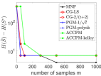
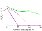
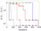
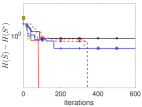
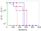
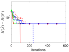
Figure 2: Noisy submodular minimization results for Genrmf-long (right) and Two-moons (left) data: Best achieved objective (log-scale) vs. number of samples (top). Objective (log-scale) vs. iterations, for $m=50$ (middle), $m=1000$ (bottom-right), and $m=150$ (bottom-left).

Figure 2 shows the gap in discrete objective value for all algorithms on the two datasets, for increasing number of samples $m$ (top), and for two fixed values of $m$, as a function of iterations (middle and bottom). We plot the best value achieved so far. As expected, the accuracy improves with more samples. In fact, this improvement is faster than the bounds in Proposition 4 and in (Blais et al., 2018). The objective values in the Two-moons data are smaller, which makes it easier to solve in the multiplicative noise setting (Prop. 4), as we indeed observe. Among the compared algorithms, ACCPM and MNP converge fastest, as also observed in (Bach, 2013) without noise, but they also seem to be the most sensitive to noise. In summary, these empirical results suggest that submodular minimization algorithms are indeed robust to noise, as predicted by our theory.

5.2 Structured sparse learning

Our second set of experiments is structured sparse learning, where we aim to estimate a sparse parameter vector $\boldsymbol{x}^{\natural}\in\mathbb{R}^{d}$ whose support is an interval. The range function $F^{r}(S)=\max(S)-\min(S)+1$ if $S\not=\emptyset$, and $F^{r}(\emptyset)=0$, is a natural regularizer to choose. $F^{r}$ is $\tfrac{1}{d-1}$-weakly DR-submodular (El Halabi et al., 2018). Another reasonable regularizer is the modified range function $F^{\mathrm{mr}}(S)=d-1+F^{r}(S),\forall S\not=\emptyset$ and $F^{\mathrm{mr}}(\emptyset)=0$, which is non-decreasing and submodular (Bach, 2010). As discussed in Section 4.1, no prior method provides a guaranteed approximate solution to Problem (3) with such regularizers, with the exception of some statistical assumptions, under which $\boldsymbol{x}^{\natural}$ can be recovered using the tightest convex relaxation $\Theta^{r}$ of $F^{r}$ (El Halabi et al., 2018). Evaluating $\Theta^{r}$ involves a linear program with constraints corresponding to all possible interval sets. Such exhaustive search is not feasible in more complex settings.

We consider a simple linear regression setting in which $\boldsymbol{x}^{\natural}\in\mathbb{R}^{d}$ has $k$ consecutive ones and is zero otherwise. We observe $\boldsymbol{y}=\boldsymbol{A}\boldsymbol{x}^{\natural}+\boldsymbol{\epsilon}$, where $\boldsymbol{A}\in\mathbb{R}^{d\times n}$ is an i.i.d Gaussian matrix with normalized columns, and $\boldsymbol{\epsilon}\in\mathbb{R}^{n}$ is an i.i.d Gaussian noise vector with standard deviation $0.01$. We set $d=250,k=20$ and vary the number of measurements $n$ between $d/4$ and $2d$. We compare the solutions obtained by minimizing the least squares loss $\ell(\boldsymbol{x})=\frac{1}{2}\|\boldsymbol{y}-\boldsymbol{A}\boldsymbol{x}\|_{2}^{2}$ with the three regularizers: The range function $F^{r}$, where $H$ is optimized via exhaustive search (OPT-Range), or via PGM (PGM-Range); the modified range function $F^{\mathrm{mr}}$, solved via exhaustive search (OPT-ModRange), or via PGM (PGM-ModRange); and the convex relaxation $\Theta^{r}$ (CR-Range), solved using CVX (Grant & Boyd, 2014). The marginal gains of $G^{\ell}$ can be efficiently computed using rank-1 updates of the pseudo-inverse (Meyer, 1973).

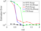
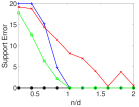
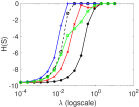
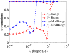
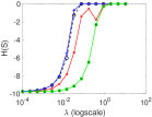
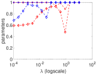
Figure 3: Structured sparsity results: Support and estimation errors (log-scale) vs measurement ratio (top); objective and corresponding $\alpha_{T},\beta_{T}$ parameters vs. regularization parameter for $n=112$ (middle) and $n=306$ (bottom).

Figure 3 (top) displays the best achieved support error in hamming distance, and estimation error $\|\hat{\boldsymbol{x}}-\boldsymbol{x}^{\natural}\|_{2}/\|\boldsymbol{x}^{\natural}\|_{2}$ on the regularization path, where $\lambda$ was varied between $10^{-4}$ and $10$. Figure 3 (middle and bottom) illustrates the objective value $H=\lambda F^{r}-G^{\ell}$ for PGM-Range, CR-Range, and OPT-Range, and $H=\lambda F^{mr}-G^{\ell}$ for PGM-ModRange, and OPT-ModRange, and the corresponding parameters $\alpha_{T},\beta_{T}$ defined in Remark 1, for two fixed values of $n$. Results are averaged over $5$ runs.

We observe that PGM minimizes the objective with $F^{mr}$ almost exactly as $n$ grows. It performs a bit worse with $F^{r}$, which is expected since $F^{r}$ is not submodular. This is also reflected in the support and estimation errors. Moreover, $\alpha_{T},\beta_{T}$ here reasonably predict the performance of PGM; larger values correlate with closer to optimal objective values. They are also more accurate than the worst case $\alpha,\beta$ in Definition 1. Indeed, the $\alpha_{T}$ for the range function is much larger than the worst case $\tfrac{1}{d-1}$. Similarly, $\beta_{T}$ for $G^{\ell}$ is quite large and approaches 1 as $n$ grows, while in Proposition 5 the worst case $\beta$ is only guaranteed to be non-zero when $\ell$ is strongly convex. Finally, the convex approach with $\Theta^{r}$ essentially matches the performance of OPT-Range when $n\geq d$. In this regime, $G^{\ell}$ becomes nearly modular, hence the convex objective $\ell+\lambda\Theta^{r}$ starts approximating the convex closure of $\lambda F^{r}-G^{\ell}$.

6 Conclusion

We established new links between approximate submodularity and convexity, and used them to analyze the performance of PGM for unconstrained, possibly noisy, non-submodular minimization. This yielded the first approximation guarantee for this problem, with a matching lower bound establishing its optimality. We experimentally validated our theory, and illustrated the robustness of submodular minimization algorithms to noise and non-submodularity.

Appendix A Extension to constrained minimization

Our result directly implies a generalization of some approximation guarantees of constrained submodular minimization to constrained weakly DR-submodular minimization. In particular, we consider the problem

$$\min_{S\in\mathcal{C}}F(S),$$ (5)

where $F$ is a monotone $\alpha$-weakly DR-submodular function and $\mathcal{C}$ denotes a family of feasible sets. We note that Theorem 1 still holds in this setting, if we project the iterates onto the convex hull $\mathrm{conv}(\mathcal{C})$ of $\mathcal{C}$. We can thus obtain a solution $\hat{\boldsymbol{s}}\in\mathrm{conv}(\mathcal{C})$ such that $f_{L}(\hat{\boldsymbol{s}})\leq\frac{F(S^{*})}{\alpha}+\epsilon$ where $S^{*}$ is the optimal solution of (5). However, the rounding in Corollary 1 does not hold anymore, since not all sup-level sets of $\hat{\boldsymbol{s}}$ will be feasible.

One rounding approach proposed in (Iyer et al., 2014) is to simply pick the smallest feasible sup-level set. Given $\boldsymbol{s}\in[0,1]^{d}$, we pick the largest $\theta\in[0,1]$ such that $S_{\theta}=\{s_{i}:s_{i}\geq\theta\}\in\mathcal{C}$. The obtained set would then satisfy $F(S_{\theta})\leq\frac{1}{\theta}f_{L}(\boldsymbol{s})$. Applying this rounding to $\hat{\boldsymbol{s}}$, we obtain $F(\hat{S}_{\theta})\leq\frac{1}{\alpha\theta}F(S^{*})+\epsilon$. In general there is no guarantee that $\theta\not=0$. But for certain constraints, such as matroid, cut and set cover constraints, Iyer et al. (2014) show that $\theta$ admits non-zero bounds (see Table 2 in (Iyer et al., 2014)).

Appendix B Proofs for Section 3

See 1

Proof.

This decomposition builds on the decomposition of $H$ into the difference of two non-decreasing submodular functions (Iyer & Bilmes, 2012). We start by choosing any function $G^{\prime}$ which is non-decreasing $(\alpha,\beta)$-weakly DR-modular, and is strictly $\alpha$-weakly DR-submodular, i.e., $\epsilon_{G^{\prime}}=\min_{i\in V,A\subset B\subseteq V\setminus i}G^{\prime}(i|A)-\alpha G^{\prime}(i|B)>0$. It is always possible to find such a function: for $\alpha=1$, we provide an example in Proposition 2. For $\alpha<1$, we can simply use $G^{\prime}(S)=|S|$. It is not possible to choose $G^{\prime}$ such that $\alpha=\beta=1$ (this would imply $G^{\prime}(i|B)\geq G^{\prime}(i|A)>G^{\prime}(i|B)$). We then construct $F$ and $G$ based on $G^{\prime}$.

Let $\epsilon_{H}=\min_{i\in V,A\subseteq B\subseteq V\setminus i}H(i|A)-\alpha H(i|B)<0$ the violation of $\alpha$-weak DR-submodularity of $H$; we may use a lower bound $\epsilon^{\prime}_{H}\leq\epsilon_{H}$. We define

$$F^{\prime}(S)=H(S)+\frac{|\epsilon^{\prime}_{H}|}{\epsilon_{G^{\prime}}}G^{\prime}(S),$$

then $F^{\prime}(i|A)\geq\alpha F^{\prime}(i|B),\forall i\in V,A\subset B\subseteq V\setminus i$, but not necessarily for $A=B$ since $F^{\prime}$ is not necessarily non-decreasing. To correct for that, let $V^{-}=\{i:F^{\prime}(i|V\setminus i)<0\}$ and define

$$F(S)=F^{\prime}(S)-\sum_{i\in S\cap V-}F^{\prime}(i|V\setminus i).$$

For all $i\in V,A\subseteq V\setminus i$, if $i\not\in V^{-}$ then $F(i|A)=F^{\prime}(i|A)\geq\alpha F^{\prime}(i|V\setminus i)\geq 0$, otherwise $F(i|A)=F^{\prime}(i|A)-F^{\prime}(i|V\setminus i)\geq(\alpha-1)F^{\prime}(i|V\setminus i)\geq 0$ for $A\not=V\setminus i$ and $F(i|V\setminus i)=0$. $F$ is thus non-decreasing $\alpha$-weakly DR-submodular. We also define

$$G(S)=\frac{|\epsilon^{\prime}_{H}|}{\epsilon_{G^{\prime}}}G^{\prime}(S)-\sum_{i\in S\cap V-}F^{\prime}(i|V\setminus i),$$

then $H(S)=F(S)-G(S)$, and $G$ is non-decreasing $(\alpha,\beta)$-weakly DR-modular. ∎

See 2

Proof.

$g$ is a concave function, since $a<0$, hence $G^{\prime}(S)$ is submodular. It also follows that

$$\max_{i\in V,S\subseteq T\subseteq V\setminus i}\frac{G^{\prime}(i|S)}{G^{\prime}(i|T)} =\max_{i\in V,S\subseteq T\subseteq V\setminus i}\frac{G^{\prime}(i)}{G^{\prime}(i|V\setminus i)}$$

$$=\frac{\tfrac{1}{2}a+(1-\tfrac{1}{2}a)}{\tfrac{1}{2}a(d^{2}-(d-1)^{2})+(1-\tfrac{1}{2}a)(d-(d-1))}$$

$$=\frac{1}{\tfrac{1}{2}a(2d-2)+1}$$

$$=\frac{1}{\beta}.$$

We also have

$$\epsilon_{G^{\prime}} =\min_{i\in V,S\subset T\subseteq V\setminus i}G^{\prime}(i|S)-G^{\prime}(i|T)$$

$$=\min_{T\subset V}2g(|T|)-g(|T|-1)-g(|T|+1)$$

$$=\min_{T\subset V}\tfrac{1}{2}a(2|T|^{2}-(|T|-1)^{2}-(|T|+1)^{2})+(1-\tfrac{1}{2}a)(2|T|-(|T|-1)-(|T|+1))$$

$$=-a.$$

∎

B.1 Proofs for Section 3.1

See 1

Proof.

Given any feasible point $(\boldsymbol{\kappa}^{\prime},\rho^{\prime})$ in the definition of $h^{-}$, i.e., $\boldsymbol{\kappa}(A)+\rho^{\prime}\leq H(A),\forall A\subseteq V$, we have:

$$\boldsymbol{\kappa}^{\top}\boldsymbol{s}-(\boldsymbol{\kappa}^{\prime\top}\boldsymbol{s}+\rho^{\prime}) =\sum_{k=1}^{d}s_{j_{k}}(H(j_{k}|S_{k-1})-\kappa^{\prime}_{j_{k}})-\rho^{\prime}$$

$$=\sum_{k=1}^{d-1}(s_{j_{k}}-s_{j_{k+1}})\left(H(S_{k})-\boldsymbol{\kappa}^{\prime}(S_{k})\right)+s_{j_{d}}\left(H(V)-\boldsymbol{\kappa}^{\prime}(V)\right)-\rho^{\prime}$$

$$\geq\left(\sum_{k=1}^{d-1}(s_{j_{k}}-s_{j_{k+1}})+s_{j_{d}}\right)\rho^{\prime}-\rho^{\prime}$$

$$=(s_{j_{1}}-1)\rho^{\prime}\geq 0$$

Hence $\boldsymbol{\kappa}^{\top}\boldsymbol{s}\geq h^{-}(\boldsymbol{s})$. The last inequality holds by noting that $\rho^{\prime}\leq 0$ since $\boldsymbol{\kappa}(\emptyset)+\rho^{\prime}\leq H(\emptyset)=0$.

The upper bound on $\boldsymbol{\kappa}(A)$ for any $A\subseteq V$ follows from the definition of weak DR-submodularity.

$$\boldsymbol{\kappa}(A) =\sum_{j_{k}\in A}H(j_{k}|S_{k-1})$$

$$\leq\sum_{j_{k}\in A}\frac{1}{\alpha}F(j_{k}|A\cap S_{k-1})-\beta G(j_{k}|A\cap S_{k-1})$$

$$=\sum_{k=1}^{d}\frac{1}{\alpha}(F(A\cap S_{k})-F(A\cap S_{k-1}))-\beta(G(A\cap S_{k})-G(A\cap S_{k-1}))$$

$$=\frac{F(A)}{\alpha}-\beta G(A)$$

Note that $\boldsymbol{\kappa}$ can be written as $\boldsymbol{\kappa}=\boldsymbol{\kappa}^{F}-\boldsymbol{\kappa}^{G}$ where $\boldsymbol{\kappa}^{F}_{j_{k}}=F(j_{k}|S_{k-1})$ and $\boldsymbol{\kappa}^{G}_{j_{k}}=G(j_{k}|S_{k-1})$. We have $\boldsymbol{\kappa}^{F}(A)\leq\frac{F(A)}{\alpha}$ and $\boldsymbol{\kappa}^{G}(A)\leq\beta G(A),\forall A\subseteq V$. Hence $(\alpha\boldsymbol{\kappa}^{F},\boldsymbol{0})$ and $(\frac{1}{\beta}\boldsymbol{\kappa}^{G},\boldsymbol{0})$ are feasible points in the definitions of $f^{-}$ and $(-g)^{-}$. The bound on $\boldsymbol{\kappa}^{\top}\boldsymbol{s}^{\prime}$ for any $\boldsymbol{s}^{\prime}\in[0,1]^{d}$ then follows directly from the definitions of $f^{-}$ and $(-g)^{-}$ (3.1). ∎

B.2 Proofs for Section 3.2

See 1

Proof.

Let $\boldsymbol{z}^{t+1}=\boldsymbol{s}^{t}-\eta\boldsymbol{\kappa}^{t}$, then note that $\|\boldsymbol{s}^{t+1}-\boldsymbol{s}^{*}\|_{2}\leq\|\boldsymbol{z}^{t+1}-\boldsymbol{s}^{*}\|_{2}$ due to the properties of projection (see for e.g., (Bubeck, 2014, Lemma 3.1)), it follows then

$$\langle\boldsymbol{\kappa}^{t},\boldsymbol{s}^{t}-\boldsymbol{s}^{*}\rangle =\frac{1}{\eta}\langle\boldsymbol{s}^{t}-\boldsymbol{z}^{t+1},\boldsymbol{s}^{t}-\boldsymbol{s}^{*}\rangle$$

$$=\frac{1}{2\eta}(\|\boldsymbol{s}^{t}-\boldsymbol{z}^{t+1}\|_{2}^{2}+\|\boldsymbol{s}^{t}-\boldsymbol{s}^{*}\|_{2}^{2}-\|\boldsymbol{z}^{t+1}-\boldsymbol{s}^{*}\|_{2}^{2})$$

$$=\frac{1}{2\eta}(\|\boldsymbol{s}^{t}-\boldsymbol{s}^{*}\|_{2}^{2}-\|\boldsymbol{z}^{t+1}-\boldsymbol{s}^{*}\|_{2}^{2})+\frac{\eta}{2}\|\boldsymbol{\kappa}^{t}\|_{2}^{2}$$

$$\leq\frac{1}{2\eta}(\|\boldsymbol{s}^{t}-\boldsymbol{s}^{*}\|_{2}^{2}-\|\boldsymbol{s}^{t+1}-\boldsymbol{s}^{*}\|_{2}^{2})+\frac{\eta}{2}\|\boldsymbol{\kappa}^{t}\|_{2}^{2}$$

Summing over $t$ we get

$$\sum_{t=1}^{T}\langle\boldsymbol{\kappa}^{t},\boldsymbol{s}^{t}-\boldsymbol{s}^{*}\rangle \leq T\frac{R^{2}}{2\eta}+\frac{\eta TL^{2}}{2}$$

Since $F$ is $\alpha$-weakly DR submodular and $-G$ is $\frac{1}{\beta}$-weakly DR submodular, we have by lemma 1 for all $t$, $(\boldsymbol{\kappa}^{t})^{\top}\boldsymbol{s}^{*}\leq\frac{f^{-}(\boldsymbol{s}^{*})}{\alpha}+\beta(-g)^{-}(\boldsymbol{s}^{*})$ and $(\boldsymbol{\kappa}^{t})^{\top}\boldsymbol{s}^{t}=h_{L}(\boldsymbol{s}^{t})\geq h^{-}(\boldsymbol{s}^{t})$. Plugging in the value of $\eta$, we thus obtain

$$\min_{t}h^{-}(\boldsymbol{s}^{t})\leq\min_{t}h_{L}(\boldsymbol{s}^{t})\leq\frac{f^{-}(\boldsymbol{s}^{*})}{\alpha}+\beta(-g)^{-}(\boldsymbol{s}^{*})+\frac{RL}{\sqrt{T}}.$$

∎

See 1

Proof.

By definition of the Lovász extension, $h_{L}(\hat{\boldsymbol{s}})=\sum_{k=1}^{d-1}(\hat{s}_{j_{k}}-\hat{s}_{j_{k+1}})H(\hat{S}_{k})+\hat{s}_{j_{d}}H(V)\geq\min_{k\in\{0,\cdots,d\}}H(\hat{S}_{k}).$ The corollary then follows by Theorem 1 and the extension property $f^{-}(\boldsymbol{s}^{*})=F(S^{*}),(-g)^{-}(\boldsymbol{s}^{*})=-G(S^{*})$. ∎

See 2

Proof.

We may write $\tilde{H}(S)=\tilde{F}(S)-\tilde{G}(S)$, where $\tilde{F}(S)=F(V\setminus S)$ is non-decreasing $1/\alpha$-weakly DR-submodular, and $\tilde{G}(S)=G(V\setminus S)$ is non-decreasing $1/\beta$-weakly DR-supermodular. Let $\tilde{S}^{*}\in\operatorname*{arg\,min}_{S\subseteq V}\tilde{H}(S)$, then $S^{*}=V\setminus\tilde{S}^{*}$. Corollary 1 implies that $H(\hat{S})=\tilde{H}(\tilde{S})\leq{\alpha}\tilde{F}(\tilde{S}^{*})-\tfrac{1}{\beta}\tilde{G}(\tilde{S}^{*})={\alpha}F(S^{*})-\tfrac{1}{\beta}G(S^{*})$. The tightness follows from Proposition 7, too. ∎

B.3 Proofs for Section 3.3

See 3

Proof.

We define $\boldsymbol{\kappa}$ as $\kappa_{j_{k}}=H(j_{k}|S_{k-1})$ and $\tilde{\boldsymbol{\kappa}}$ as $\tilde{\kappa}_{j_{k}}=\tilde{H}(j_{k}|S_{k-1})$ for any ordering on $V$. For all $k\in V$, we have $|\tilde{\kappa}_{j_{k}}-\kappa_{j_{k}}|\leq 2\epsilon$ with probability $1-2d\delta$ (by a union bound), hence $|\boldsymbol{\tilde{\kappa}}(S^{*})-\boldsymbol{\kappa}(S^{*})|\leq 2\epsilon|S^{*}|$. Plugging this into the proofs of Theorem 1 and Corollary 1 yields $H(\hat{S})\leq\tfrac{1}{\alpha}F(S^{*})-\beta G(S^{*})+2\epsilon(|S^{*}|+1)+\tfrac{RL}{\sqrt{T}},$ with probability $1-2dT\delta$ (by a union bound). The proposition follows by setting $\epsilon,\delta$ and $T$ to the chosen values. ∎

See 4

Proof.

For every $S\subseteq V$ and $\epsilon^{\prime}>0$, a Chernoff bound implies that $(1-\epsilon^{\prime})\mu H(S)\leq\tilde{H}_{m}(S)=\tfrac{1}{m}\sum_{i=1}^{m}\xi_{i}H(S)\leq(1+\epsilon^{\prime})\mu H(S),$ with probability at least $1-\exp(-\tfrac{\epsilon^{\prime 2}\mu^{2}m}{\omega^{2}})$. Choosing $\epsilon^{\prime}=\tfrac{\epsilon}{\mu H_{\max}}$ yields the proposition. ∎

B.4 Proofs for Section 3.4

See 2

Proof.

Let $C,D$ be two sets that partition the ground set $V=C\cup D$ such that $|C|=|D|=d/2$. We construct a normalized set function $H$ whose values depend only on $k(S)=|S\cap C|$ and $\ell(S)=|S\cap D|$. In particular, we define

$$H(S)=\begin{cases}0&\text{if $|k(S)-\ell(S)|\leq\epsilon d$}\\ \frac{2\alpha\delta}{2-d}&\text{otherwise}\end{cases},$$

for some $\epsilon\in[1/d,1/2)$. By Proposition 1, given a non-decreasing $(\alpha,\beta)$-weakly DR-modular function $G^{\prime}$, we can write $H(S)=F(S)-G(S)$, where $F(S)=H(S)+\frac{|\epsilon_{H}|}{\epsilon_{G^{\prime}}}G^{\prime}(S)$ is normalized non-decreasing $\alpha$-weakly DR-submodular, and $G(S)=\frac{|\epsilon_{H}|}{\epsilon_{G^{\prime}}}G^{\prime}(S)$ is normalized non-decreasing $(\alpha,\beta)$-weakly DR-modular. Note that $V^{-}=\emptyset$ in this case, since $H(i|V\setminus i)=0$. We choose $G^{\prime}(S)=|S|$ if $\alpha<1$, then $\epsilon_{G^{\prime}}=\min_{i\in V,S\subset T\subseteq T\setminus i}G(i|S)-\alpha G(i|T)=1-\alpha>0$. If $\alpha=1$, we use the $(1,\beta)$-weakly DR-modular function defined in Proposition 2, then $\epsilon_{G^{\prime}}=\frac{1-\beta}{d-1}>0$.

Let the partition $(C,D)$ be random and unknown to the algorithm. We argue that, with high probability, any given query $S$ will be “balanced”, i.e., $|k(S)-\ell(S)|\leq\epsilon d$. Hence no deterministic algorithm can distinguish between $H$ and the constant zero function. Given a fixed $S\subseteq V$, let $X_{i}=1$ if $i\in C$ and $0$ otherwise, for all $i\in S$, then $\mu=\mathbb{E}[\sum_{i\in S}X_{i}]=\sum_{i\in S}\frac{|C|}{d}=\frac{|S|}{2}$. Then by a Chernoff’s bound we have $Pr(|k(S)-\ell(S)|>\epsilon d)\leq 2\exp(-\frac{\epsilon^{2}d}{4})$. Hence, given a sequence of $e^{\frac{\epsilon^{2}d}{8}}$ queries, the probability that each query $S$ is balanced, and thus has value $H(S)=0$, is still at least $1-2e^{-\frac{\epsilon^{2}d}{8}}$. On the other hand, we have $H(S^{*})=\frac{2\alpha\delta}{2-d}<0$, achieved at $S^{*}=C$ or $D$. Moreover, note that $\epsilon_{H}=\min_{i\in V,S\subseteq T\subseteq T\setminus i}H(i|S)-\alpha H(i|T)=(1+\alpha)H(S^{*})$. Hence

$$\tfrac{1}{\alpha}F(S^{*})-\beta G(S^{*})-\delta=\tfrac{1}{\alpha}H(S^{*})\biggl{(}1-(1-\alpha\beta)(1+\alpha)\frac{G^{\prime}(S^{*})}{\epsilon_{G^{\prime}}}\biggl{)}-\delta<0,$$

since $\tfrac{G^{\prime}(S^{*})}{\epsilon_{G^{\prime}}}=\tfrac{d}{2(1-\alpha)}$ if $\alpha<1$, and $\frac{G^{\prime}(S^{*})}{\epsilon_{G^{\prime}}}\geq\frac{3d(d-1)}{8(1-\beta)}$, if $\alpha=1$.

Therefore, with high probability, the algorithm cannot find a set with value $H(S)\leq\tfrac{1}{\alpha}F(S^{*})-\beta G(S^{*})-\delta$. This also holds for a randomized algorithm, by averaging over its random choices. ∎

Proposition 7 (Tight example for PGM).

For any $\alpha,\beta\in(0,1]$, there exists a set function $H(S)=F(S)-G(S)$, where $F$ is a non-decreasing $(\alpha,1)$-weakly DR-modular function and $G$ is a non-decreasing $(1,\beta)$-weakly DR-modular function, such that the solution $\hat{S}$ in Corollary 1 satisfies $H(\hat{S})=F(S^{*})/\alpha-\beta G(S^{*}).$

Proof.

We define

$$F(S)=\begin{cases}|S|+\tfrac{d}{\beta}-1&\text{if $1\in S$}\\ \alpha|S|&\text{ otherwise}\end{cases},\text{ and }G(S)=\begin{cases}|S|+\tfrac{d}{\beta}-1&\text{if $1\in S$}\\ \tfrac{1}{\beta}|S|&\text{ otherwise}\end{cases}.$$

It’s easy to see that both $F$ and $G$ are monotone functions. For all $A\subseteq B,i\in V\setminus B$, we have

$$\frac{F(i|A)}{F(i|B)}=\begin{cases}1&\text{if $1\in A$ or $1\not\in B$}\\ \alpha&\text{if $1\not\in A,1\in B$}\\ \frac{\frac{d}{\beta}+(1-\alpha)|A|}{\frac{d}{\beta}+(1-\alpha)|B|}&\text{if $i=1$}\\ \end{cases}$$

Note that $\frac{d}{\beta}+(1-\alpha)|A|\geq\frac{d}{\beta}\geq\alpha(\frac{d}{\beta}+(1-\alpha)|B|)$, hence $\alpha\leq\frac{F(i|A)}{F(i|B)}\leq 1$, which proves that $F$ is supermodular and $\alpha$-weakly DR-submodular.

Similarly we have

$$\frac{F(i|A)}{F(i|B)}=\begin{cases}1&\text{if $1\in A$ or $1\not\in B$}\\ \frac{1}{\beta}&\text{if $1\not\in A,1\in B$}\\ \frac{\frac{d}{\beta}+(1-\frac{1}{\beta})|A|}{\frac{d}{\beta}+(1-\frac{1}{\beta})|B|}&\text{if $i=1$}\\ \end{cases}$$

Note that $\frac{d}{\beta}+(1-\frac{1}{\beta})|A|\leq\frac{d}{\beta}\leq\frac{1}{\beta}(\frac{d}{\beta}+(1-\frac{1}{\beta})|B|)$, hence $1\leq\frac{F(i|A)}{F(i|B)}\leq\frac{1}{\beta}$, which proves that $G$ is monotone submodular and $\beta$-weakly DR-supermodular.

It remains to show that the solution obtained by projected subgradient method and thresholding have value $H(\hat{S})=0$. We can assume w.l.o.g that the starting point $\boldsymbol{s}^{1}$ is such that the largest element is $j_{1}=1$ (otherwise we can modify the example to have whatever is the largest element as the “bad element”). Note that $H(1)=H(j_{k}|S_{k})=0$ for all $k\in[d]$, hence $\boldsymbol{\kappa}^{1}=\mathbf{0}$ and $\boldsymbol{s}^{t}=\boldsymbol{s}^{1}$ and $\boldsymbol{\kappa}^{t}=\mathbf{0}$ for all $t\in\{1,\cdots,T\}$. Thresholding $\boldsymbol{s}^{1}$ would thus yield $H(\hat{S})=0$, with $\hat{S}=\emptyset$ or any other set such that $1\in\hat{S}$. ∎

Appendix C Proofs for Section 4

C.1 Proofs for Section 4.1

We actually prove Proposition 5 under a more general setting: if $\ell$ has $\nu$-restricted smoothness (RSM) and $\mu$-restricted strong convexity (RSC) on the domain of $k$-sparse vectors, $G^{\ell}$ is weakly DR-modular for all sets of cardinality $k$. Our current algorithm analysis requires weak DR-submodularity to hold for all sets. Whether the algorithm can be modified to only query sets of cardinality $k$ is an interesting question for future work. Let’s recall the definition of RSC/RSM.

Definition 3 (RSM/RSC).

Given a differentiable function $\ell:\mathbb{R}^{d}\to\mathbb{R}$ and $\Omega\subset\mathbb{R}^{d}\times\mathbb{R}^{d}$, $\ell$ is $\mu_{\Omega}$-RSC and $\nu_{\Omega}$-RSM if $\frac{\mu_{\Omega}}{2}\|\boldsymbol{x}-\boldsymbol{y}\|_{2}^{2}\leq\ell(\boldsymbol{y})-\ell(\boldsymbol{x})-\langle\nabla\ell(\boldsymbol{x}),\boldsymbol{y}-\boldsymbol{x}\rangle\leq\frac{\nu_{\Omega}}{2}\|\boldsymbol{x}-\boldsymbol{y}\|_{2}^{2},\;\;\forall(\boldsymbol{x},\boldsymbol{y})\in\Omega.$

If $\ell$ is RSC/RSM on $\Omega=\{(\boldsymbol{x},\boldsymbol{y}):\|\boldsymbol{x}\|_{0}\leq k_{1},\|\boldsymbol{y}\|_{0}\leq k_{1},\|\boldsymbol{x}-\boldsymbol{y}\|_{0}\leq k_{2}\}$, we denote by $\mu_{k_{1},k_{2}},\nu_{k_{1},k_{2}}$ the corresponding RSC and RSM parameters. For simplicity, we also define $\mu_{k}:=\mu_{k,k},\nu_{k}:=\mu_{k,k}$.

Before we can prove Proposition 5, we need two key lemmas. Lemma 2 restates a result from (Elenberg et al., 2018), which relates the marginal gain of $G^{\ell}$ to the marginal decrease in $\ell$. In Lemma 3, we argue that for a class of loss functions, namely RSC/RSM functions of the form $\ell(\boldsymbol{x})=L(\boldsymbol{x})-\boldsymbol{z}^{\top}\boldsymbol{x}$, where $\boldsymbol{z}$ is a random vector, the corresponding minimizer has full support with probability one. Proposition 8 then follows from these two lemmas by noting that $\ell$ thus have non-zero marginal decrease, with respect to any $i\in V$, with probability one.

Lemma 2.

Given $G^{\ell}(S)=\ell(0)-\min_{\mathrm{supp}(\boldsymbol{x})\subseteq S}\ell(\boldsymbol{x})$, then for any disjoint sets $A,B\subseteq V$ and a corresponding minimizer $\boldsymbol{x}^{A}:=\operatorname*{arg\,min}_{\mathrm{supp}(\boldsymbol{x})\subseteq A}\ell(\boldsymbol{x})$, if $\ell$ is $\mu_{|A\cup B|}$-RSC and $\nu_{|A|,|B|}$-RSM, we have:

$$\frac{\|[\nabla\ell(\boldsymbol{x}^{A})]_{B}\|_{2}^{2}}{2\nu_{|A\cup B|,|B|}}\leq G^{\ell}(B|A)\leq\frac{\|[\nabla\ell(\boldsymbol{x}^{A})]_{B}\|_{2}^{2}}{2\mu_{|A\cup B|}}$$

Lemma 3.

If $\boldsymbol{x}^{\star}$ is the minimizer of $\min_{x\in\mathbb{R}^{d}}L(\boldsymbol{x})-\boldsymbol{z}^{\top}\boldsymbol{x}$, where $L$ is a strongly-convex and smooth loss function, and $\boldsymbol{z}\in\mathbb{R}^{d}$ has a continuous density w.r.t to the Lebesgue measure, then $\boldsymbol{x}^{\star}$ has full support with probability one.

Proof.

This follows directly from (El Halabi et al., 2018, Theorem 1) by taking $\Phi(x)=0$. We include the proof here for completeness.

Since $L$ is strongly-convex, given $\boldsymbol{z}$ the corresponding minimizer $\boldsymbol{x}^{\star}$ is unique, then the function $E(\boldsymbol{z}):=\operatorname*{arg\,min}_{\boldsymbol{x}\in\mathbb{R}^{d}}L(\boldsymbol{x})-\boldsymbol{z}^{T}\boldsymbol{x}$ is well defined. Given fixed $i\in V$, we show that the set $S_{i}:=\{\boldsymbol{z}:[E(\boldsymbol{z})]_{i}=0\}$ has measure zero. Then, taking the union of the finitely many sets $S_{i},\forall i\in V$, all of zero measure, we have $P(\exists\boldsymbol{z}\in\mathbb{R}^{d},\exists i\in V,\text{ s.t., }[E(\boldsymbol{z})]_{i}=0)=0$.

To show that the set $S_{i}$ has measure zero, let $\boldsymbol{z}_{1},\boldsymbol{z}_{2}\in S_{i}$ and denote by $\mu>0$ the strong convexity constant of $L$. We have by optimality conditions:

$$\Big{(}\big{(}\boldsymbol{z}_{1}-\nabla L(E(\boldsymbol{z}_{1}))\big{)}-\big{(}\boldsymbol{z}_{2}-\nabla L(E(\boldsymbol{z}_{2}))\big{)}\Big{)}^{\top}\Big{(}E(\boldsymbol{z}_{1})-E(\boldsymbol{z}_{2})\Big{)}=0$$

Hence,

$$(\boldsymbol{z}_{1}-\boldsymbol{z}_{2})^{\top}(E(\boldsymbol{z}_{1})-E(\boldsymbol{z}_{2})) \geq\big{(}\nabla L(E(\boldsymbol{z}_{1}))-\nabla L(E(\boldsymbol{z}_{2}))\big{)}^{\top}\big{(}E(\boldsymbol{z}_{1})-E(\boldsymbol{z}_{2})\big{)}$$

$$(\boldsymbol{z}_{1}-\boldsymbol{z}_{2})^{\top}(E(\boldsymbol{z}_{1})-E(\boldsymbol{z}_{2})) \geq\mu\|E(\boldsymbol{z}_{1})-E(\boldsymbol{z}_{2})\|_{2}^{2}$$

$$\frac{1}{\mu}\|\boldsymbol{z}_{1}-\boldsymbol{z}_{2}\|_{2} \geq\|E(\boldsymbol{z}_{1})-E(\boldsymbol{z}_{2})\|_{2}$$

Thus $E$ is a deterministic Lipschitz-continuous function of $\boldsymbol{z}$. By optimality conditions $\boldsymbol{z}=\nabla L(E(\boldsymbol{z}))$, then $z_{i}=\nabla L(E(\boldsymbol{z}_{V\setminus i}))_{i}$. Thus $z_{i}$ is a Lipschitz-continuous function of $\boldsymbol{z}_{V\setminus i}$, which can only happen with zero measure. ∎

Proposition 8.

Let $\ell(\boldsymbol{x})=L(\boldsymbol{x})-\boldsymbol{z}^{\top}\boldsymbol{x}$, where $L$ is $\mu_{|U|}$-RSC and $\nu_{|U|}$-RSM for some $U\subseteq V$ and $\boldsymbol{z}\in\mathbb{R}^{d}$ has a continuous density w.r.t the Lebesgue measure. Then there exist $\alpha_{G},\beta_{G}>0$ such that $G^{\ell}$ is $(\alpha_{G},\beta_{G})$-weakly DR modular on $U$ (i.e., Def. 1 restricted to sets $A\subseteq B\subseteq U$).

Proof.

Given $i\in U,A\subseteq U\setminus i$, let $\boldsymbol{x}^{A}:=\operatorname*{arg\,min}_{\mathrm{supp}(\boldsymbol{x})\subseteq A}\ell(\boldsymbol{x})$, then by Lemma 2 and $\nu_{|A|+1,1}\leq\nu_{|A|+1}$ we have:

$$\frac{[\nabla\ell(\boldsymbol{x}^{A})]_{i}^{2}}{2\nu_{|A|+1}} \leq G^{\ell}(i|A)\leq\frac{[\nabla\ell(\boldsymbol{x}^{A})]_{i}^{2}}{2\mu_{|A|+1}}$$

We argue that $[\nabla\ell(x^{A})]_{i}^{2}\not=0$ with probability one. For that, we define $\ell_{A}(\boldsymbol{u}):=\ell(\boldsymbol{x})$, where $[\boldsymbol{x}]_{A}=\boldsymbol{u},[\boldsymbol{x}]_{V\setminus A}=0,\forall\boldsymbol{u}\in\mathbb{R}^{|A|}$, then $\ell_{A}$ is $\mu_{|A|}$-strongly convex and $\nu_{|A|}$-smooth on $\mathbb{R}^{|A|}$. Hence, by lemma 3, the minimizer $\boldsymbol{u}^{\star}$ of $\ell_{A}$ has full support with probability one, and thus $\mathrm{supp}(\boldsymbol{x}^{A})=A$ also with probability one. By the same argument, we have $\mathrm{supp}(\boldsymbol{x}^{A\cup\{i\}})=A\cup\{i\}$. We can thus deduce that $[\nabla\ell(x^{A})]_{i}^{2}\not=0$, since otherwise $G^{\ell}(i|A)=0$, which implies that $\boldsymbol{x}^{A\cup\{i\}}=x^{A}$ (minimizer is unique) and $\mathrm{supp}(\boldsymbol{x}^{A\cup\{i\}})=A$, which happens with probability zero.

For all $i\in U,A,B\subseteq U\setminus i$, the following bounds hold:

$$\frac{\mu_{|B|+1}[\nabla\ell(\boldsymbol{x}^{A})]_{i}^{2}}{\nu_{|A|+1}[\nabla\ell(\boldsymbol{x}^{B})]_{i}^{2}}\leq\frac{G^{\ell}(i|A)}{G^{\ell}(i|B)}\leq\frac{\nu_{|B|+1}[\nabla\ell(\boldsymbol{x}^{A})]_{i}^{2}}{\mu_{|A|+1}[\nabla\ell(\boldsymbol{x}^{B})]_{i}^{2}}$$

$G^{\ell}$ is then $(\alpha_{G},\beta_{G})$-weakly DR-modular with $\alpha_{G}:=\min_{A\subseteq B\subseteq U,i\in U\setminus B}\frac{\mu_{|B|+1}[\nabla\ell(\boldsymbol{x}^{A})]_{i}^{2}}{\nu_{|A|+1}[\nabla\ell(\boldsymbol{x}^{B})]_{i}^{2}}>0$ and $\beta_{G}:=\min_{A\subseteq B\subseteq U,i\in U\setminus B}\frac{\mu_{|A|+1}[\nabla\ell(\boldsymbol{x}^{B})]_{i}^{2}}{\nu_{|B|+1}[\nabla\ell(\boldsymbol{x}^{A})]_{i}^{2}}>0$. ∎

C.2 Proofs for Section 4.2

To prove Proposition 6, we first show that the objective in noisy column subset selection problems is weakly DR-modular, generalizing the result of (Sviridenko et al., 2017). We then show that the variance reduction function can be written as a noisy column subset selection objective.

We start by giving explicit expressions for the marginals of the objective in noisy column subset selection problems.

Proposition 9.

Let $\ell(\boldsymbol{x}):=\frac{1}{2}\|\boldsymbol{y}-\boldsymbol{A}\boldsymbol{x}\|_{2}^{2}+\frac{\sigma^{2}}{2}\|\boldsymbol{x}\|^{2}$ for some $\sigma\geq 0$ and $G(S)=\ell(0)-\min_{\mathrm{supp}(\boldsymbol{x})\subseteq S}\ell(\boldsymbol{x})$, then

$$G(i|S) =[\boldsymbol{x}^{S\cup i}(\boldsymbol{y})]^{2}_{i}~{}\phi(S,i)=\Bigl{(}\frac{\boldsymbol{y}^{\top}R^{S}(\boldsymbol{a}_{i})}{2\sqrt{\phi(S,i)}}\Bigl{)}^{2},$$

where $\boldsymbol{a}_{i}$ is the ith column of $\boldsymbol{A}$, $\boldsymbol{x}^{S}(\boldsymbol{a}_{i}):=\operatorname*{arg\,min}_{\mathrm{supp}(\boldsymbol{x})\subseteq S}\frac{1}{2}\|\boldsymbol{a}_{i}-\boldsymbol{A}\boldsymbol{x}\|_{2}^{2}+\frac{\sigma^{2}}{2}\|\boldsymbol{x}\|^{2}$ is the vector of optimal regression coefficients, $R^{S}(\boldsymbol{a}_{i})=\boldsymbol{a}_{i}-\boldsymbol{A}\boldsymbol{x}^{S}(\boldsymbol{a}_{i})$ the corresponding residual, and $\phi(S,i)=\frac{1}{2}\|R^{S}(\boldsymbol{a}_{i})\|^{2}+\frac{\sigma^{2}}{2}\|\boldsymbol{x}^{S}(\boldsymbol{a}_{i})\|^{2}+\frac{\sigma^{2}}{2}$.

Proof.

Given $i\in V,S\subseteq V\setminus i$, let $\boldsymbol{x}^{S}(\boldsymbol{y}):=\operatorname*{arg\,min}_{\mathrm{supp}(\boldsymbol{x})\subseteq S}\ell(\boldsymbol{x})$, and $R^{S}(\boldsymbol{y})=\boldsymbol{y}-\boldsymbol{A}\boldsymbol{x}^{S}(\boldsymbol{y})$ the corresponding residual. Let $\gamma=[\boldsymbol{x}^{S\cup i}(\boldsymbol{y})]_{i}$, then we can write

$$\boldsymbol{y} =\boldsymbol{A}\boldsymbol{x}^{S\cup i}(\boldsymbol{y})+R^{S\cup i}(\boldsymbol{y})$$

$$=\boldsymbol{A}_{S}[\boldsymbol{x}^{S\cup i}(\boldsymbol{y})]_{S}+\boldsymbol{a}_{i}\gamma+R^{S\cup i}(\boldsymbol{y})$$

$$=\boldsymbol{A}_{S}([\boldsymbol{x}^{S\cup i}(\boldsymbol{y})]_{S}+\gamma\boldsymbol{x}^{S}(\boldsymbol{a}_{i}))+\gamma R^{S}(\boldsymbol{a}_{i})+R^{S\cup i}(\boldsymbol{y})$$

By optimality conditions we have $-\boldsymbol{A}_{S\cup i}^{\top}R^{S\cup i}(\boldsymbol{y})+\sigma^{2}\boldsymbol{x}^{S\cup i}(\boldsymbol{y})=0$ and $-\boldsymbol{A}_{S}^{\top}R^{S}(\boldsymbol{a}_{i})+\sigma^{2}\boldsymbol{x}^{S}(\boldsymbol{a}_{i})=0$. Let $\hat{\boldsymbol{x}}^{S}(\boldsymbol{y})=[\boldsymbol{x}^{S\cup i}(\boldsymbol{y})]_{S}+\gamma\boldsymbol{x}^{S}(\boldsymbol{a}_{i})$, then $\hat{\boldsymbol{x}}^{S}(\boldsymbol{y})$ satisfies the constraint $\mathrm{supp}(\hat{\boldsymbol{x}}^{S}(\boldsymbol{y}))=S$ and the optimality condition $\boldsymbol{A}_{S}^{\top}(\boldsymbol{A}_{S}\hat{\boldsymbol{x}}^{S}(\boldsymbol{y})-\boldsymbol{y})+\sigma^{2}\hat{\boldsymbol{x}}^{S}(\boldsymbol{y})=0$. We can see this by plugging in the expression for $\boldsymbol{y}$ and using the optimality conditions on $\boldsymbol{x}^{S\cup i}(\boldsymbol{y})$ and $\boldsymbol{x}^{S}(\boldsymbol{a}_{i})$.

$$\boldsymbol{A}_{S}^{\top}(\boldsymbol{A}_{S}\hat{\boldsymbol{x}}^{S}(\boldsymbol{y})-\boldsymbol{y})+\sigma^{2}\hat{\boldsymbol{x}}^{S}(\boldsymbol{y}) =-\boldsymbol{A}_{S}^{\top}(\gamma R^{S}(\boldsymbol{a}_{i})+R^{S\cup i}(\boldsymbol{y}))+\sigma^{2}([\boldsymbol{x}^{S\cup i}(\boldsymbol{y})]_{S}+\gamma\boldsymbol{x}^{S}(\boldsymbol{a}_{i}))=0$$

Hence $\hat{\boldsymbol{x}}^{S}(\boldsymbol{y})={\boldsymbol{x}}^{S}(\boldsymbol{y})$. By the optimality condition on $\boldsymbol{x}^{S\cup i}(\boldsymbol{y})$, we also have

$$R^{S}(\boldsymbol{a}_{i})^{\top}R^{S\cup i}(\boldsymbol{y}) =\boldsymbol{a}_{i}^{\top}R^{S\cup i}(\boldsymbol{y})-\boldsymbol{x}^{S}(\boldsymbol{a}_{i})^{\top}\boldsymbol{A}_{S}^{\top}R^{S\cup i}(\boldsymbol{y})$$

$$=\sigma^{2}\gamma-\sigma^{2}\boldsymbol{x}^{S}(\boldsymbol{a}_{i})^{\top}[\boldsymbol{x}^{S\cup i}(\boldsymbol{y})]_{S}$$

The marginals are thus given by

$$G(i|S) =\ell({\boldsymbol{x}}^{S}(\boldsymbol{y}))-\ell(\boldsymbol{x}^{S\cup i}(\boldsymbol{y}))$$

$$=\frac{1}{2}\|\gamma R^{S}(\boldsymbol{a}_{i})+R^{S\cup i}(\boldsymbol{y})\|_{2}^{2}+\frac{\sigma^{2}}{2}\|[\boldsymbol{x}^{S\cup i}(\boldsymbol{y})]_{S}+\gamma\boldsymbol{x}^{S}(\boldsymbol{a}_{i})\|^{2}-\frac{1}{2}\|R^{S\cup i}(\boldsymbol{y})\|_{2}^{2}-\frac{\sigma^{2}}{2}\|\boldsymbol{x}^{S\cup i}(\boldsymbol{y})\|^{2}$$

$$=\frac{\gamma^{2}}{2}\|R^{S}(\boldsymbol{a}_{i})\|^{2}+\sigma^{2}\gamma^{2}-\sigma^{2}\gamma\boldsymbol{x}^{S}(\boldsymbol{a}_{i})^{\top}[\boldsymbol{x}^{S\cup i}(\boldsymbol{y})]_{S}+\frac{\sigma^{2}}{2}\gamma^{2}\|\boldsymbol{x}^{S}(\boldsymbol{a}_{i})\|^{2}+\sigma^{2}\gamma\boldsymbol{x}^{S}(\boldsymbol{a}_{i})^{\top}[\boldsymbol{x}^{S\cup i}(\boldsymbol{y})]_{S}-\frac{\sigma^{2}}{2}\gamma^{2}$$

$$=\gamma^{2}(\frac{1}{2}\|R^{S}(\boldsymbol{a}_{i})\|^{2}+\frac{\sigma^{2}}{2}\|\boldsymbol{x}^{S}(\boldsymbol{a}_{i})\|^{2}+\frac{\sigma^{2}}{2})$$

Hence $G(i|S)=[\boldsymbol{x}^{S\cup i}(\boldsymbol{y})]^{2}_{i}\phi(S,i)$.

By the optimality condition on $\boldsymbol{x}^{S}(\boldsymbol{a}_{i})$ we also have:

$$~{}~{}~{}~{}~{}\frac{1}{2}\boldsymbol{y}^{\top}R^{S}(\boldsymbol{a}_{i})$$

$$=\frac{1}{2}(R^{S\cup i}(\boldsymbol{y})+\boldsymbol{A}_{S\cup i}\boldsymbol{x}^{S\cup i}(\boldsymbol{y}))^{\top}R^{S}(\boldsymbol{a}_{i})$$

$$=\frac{1}{2}\Bigl{(}\sigma^{2}\gamma-\sigma^{2}\boldsymbol{x}^{S}(\boldsymbol{a}_{i})^{\top}[\boldsymbol{x}^{S\cup i}(\boldsymbol{y})]_{S}+[\boldsymbol{x}^{S\cup i}(\boldsymbol{y})]_{S}^{\top}\boldsymbol{A}_{S}^{\top}R^{S}(\boldsymbol{a}_{i})+[\boldsymbol{x}^{S\cup i}(\boldsymbol{y})]_{i}^{\top}\boldsymbol{a}_{i}^{\top}R^{S}(\boldsymbol{a}_{i})\Bigl{)}$$

$$=\frac{1}{2}\Bigl{(}\sigma^{2}\gamma-\sigma^{2}\boldsymbol{x}^{S}(\boldsymbol{a}_{i})^{\top}[\boldsymbol{x}^{S\cup i}(\boldsymbol{y})]_{S}+\sigma^{2}[\boldsymbol{x}^{S\cup i}(\boldsymbol{y})]_{S}^{\top}\boldsymbol{x}^{S}(\boldsymbol{a}_{i})+[\boldsymbol{x}^{S\cup i}(\boldsymbol{y})]_{i}(R^{S}(\boldsymbol{a}_{i})+\boldsymbol{A}_{S}\boldsymbol{x}^{S}(\boldsymbol{a}_{i}))^{\top}R^{S}(\boldsymbol{a}_{i})\Bigl{)}$$

$$=\frac{1}{2}\Bigl{(}\sigma^{2}\gamma+\gamma\|R^{S}(\boldsymbol{a}_{i})\|_{2}^{2}+\gamma\sigma^{2}\|\boldsymbol{x}^{S}(\boldsymbol{a}_{i})\|_{2}^{2}\Bigl{)}$$

Hence $\Bigl{(}\frac{\boldsymbol{y}^{\top}R^{S}(\boldsymbol{a}_{i})}{2\sqrt{\phi(S,i)}}\Bigl{)}^{2}=\gamma^{2}{\phi(S,i)}=G(i|S)$. ∎

Proposition 10.

Given a positive-definite matrix $\boldsymbol{A}$, let $\boldsymbol{a}_{i}$ be the ith column of $\boldsymbol{A}$, and $\ell_{i}(\boldsymbol{x}):=\frac{1}{2}\|\boldsymbol{a}_{i}-\boldsymbol{A}\boldsymbol{x}\|_{2}^{2}+\frac{\sigma^{2}}{2}\|\boldsymbol{x}\|^{2}$ for all $i\in V$, for some $\sigma\geq 0$. Then the function $G(S)=\sum_{i\in V}\ell(0)-\min_{\mathrm{supp}(\boldsymbol{x})\subseteq S}\ell_{i}(\boldsymbol{x})$ is a non-decreasing $(\beta,\beta)$-weakly DR-modular function, with $\beta=(\frac{\lambda^{2}_{\min}(\boldsymbol{A})}{\sigma^{2}+\lambda^{2}_{\min}(\boldsymbol{A})})^{2}\frac{1}{\kappa^{2}(\boldsymbol{A})}$, where $\kappa(\boldsymbol{A})=\lambda_{\max}(\boldsymbol{A})/\lambda_{\min}(\boldsymbol{A})$ is the condition number of $\boldsymbol{A}$.

Proof.

For all $j\in V$, let $G_{j}(S):=\ell(0)-\min_{\mathrm{supp}(\boldsymbol{x})\subseteq S}\ell_{j}(\boldsymbol{x})$, then we can write $G(S)=\sum_{j\in V}G_{j}(S)$. Given $i\in V,S\subseteq V\setminus i$, let $\boldsymbol{x}^{S}(\boldsymbol{a}_{i}):=\operatorname*{arg\,min}_{\mathrm{supp}(\boldsymbol{x})\subseteq S}\ell_{i}(\boldsymbol{x})$ be the optimal regression coefficients, $R^{S}(\boldsymbol{a}_{i})=\boldsymbol{a}_{i}-\boldsymbol{A}\boldsymbol{x}^{S}(\boldsymbol{a}_{i})$ the corresponding residual. By Proposition 9, we have for all $j\in V$:

$$G_{j}(i|S) =[\boldsymbol{x}^{S\cup i}(\boldsymbol{a}_{j})]^{2}_{i}~{}\phi(S,i)=\Bigl{(}\frac{\boldsymbol{a}_{j}^{\top}R^{S}(\boldsymbol{a}_{i})}{2\sqrt{\phi(S,i)}}\Bigl{)}^{2},$$

where $\phi(S,i)=\frac{1}{2}\|R^{S}(\boldsymbol{a}_{i})\|^{2}+\frac{\sigma^{2}}{2}\|\boldsymbol{x}^{S}(\boldsymbol{a}_{i})\|^{2}+\frac{\sigma^{2}}{2}$. Note that $\phi(S,i)>0$ since $\boldsymbol{A}$ is positive definite (columns are linearly independent).

In the noiseless case $\sigma=0$, we have $\boldsymbol{x}^{S\cup i}(\boldsymbol{a}_{i})=\mathds{1}_{i}$. In the noisy case $\sigma>0$, we have by optimality conditions

$$(\boldsymbol{A}_{S\cup i}^{\top}\boldsymbol{A}_{S\cup i}+\sigma^{2}I)\boldsymbol{x}^{S\cup i}(\boldsymbol{a}_{i}) =\boldsymbol{A}_{S\cup i}^{\top}\boldsymbol{a}_{i}$$

$$(\boldsymbol{A}_{S\cup i}^{\top}\boldsymbol{A}_{S\cup i}+\sigma^{2}I)\boldsymbol{x}^{S\cup i}(\boldsymbol{a}_{i}) =(\boldsymbol{A}_{S\cup i}^{\top}\boldsymbol{A}_{S\cup i}+\sigma^{2}I)\mathds{1}_{i}-\sigma^{2}\mathds{1}_{i}$$

$$\boldsymbol{x}^{S\cup i}(\boldsymbol{a}_{i}) =\mathds{1}_{i}-\sigma^{2}(\boldsymbol{A}_{S\cup i}^{\top}\boldsymbol{A}_{S\cup i}+\sigma^{2}I)^{-1}\mathds{1}_{i}$$

Since $(\sigma^{2}+\lambda^{2}_{\min}(\boldsymbol{A}))^{-1}I\succcurlyeq(\boldsymbol{A}_{S\cup i}^{\top}\boldsymbol{A}_{S\cup i}+\sigma^{2}I)^{-1}\succcurlyeq(\sigma^{2}+\lambda^{2}_{\max}(\boldsymbol{A}))^{-1}I$, we have

$$1-\frac{\sigma^{2}}{\sigma^{2}+\lambda^{2}_{\min}(\boldsymbol{A})}\leq[\boldsymbol{x}^{S\cup i}(\boldsymbol{a}_{i})]_{i}\leq 1-\frac{\sigma^{2}}{\sigma^{2}+\lambda^{2}_{\max}(\boldsymbol{A})}.$$

We will construct two unit vectors $\boldsymbol{y},\boldsymbol{z}$ such that $\tfrac{1}{2}(\frac{\lambda^{2}_{\min}(\boldsymbol{A})}{\sigma^{2}+\lambda^{2}_{\min}(\boldsymbol{A})})^{2}\|\boldsymbol{A}\boldsymbol{y}\|^{2}_{2}\leq G(i|S)\leq\frac{1}{2}\|\boldsymbol{A}\boldsymbol{z}\|^{2}_{2}$.

Let $w_{j}=\frac{\boldsymbol{a}_{j}^{\top}R^{S}(\boldsymbol{a}_{i})}{2\sqrt{\phi(S,i)}},\forall j\in V$ and $\boldsymbol{z}=\boldsymbol{w}/\|\boldsymbol{w}\|_{2}$. Hence $\|\boldsymbol{z}\|_{2}=1$ and

$$\tfrac{1}{2}R^{S}(\boldsymbol{a}_{i})^{\top}\boldsymbol{A}\boldsymbol{z} =\tfrac{1}{2}\sum_{j\in V}R^{S}(\boldsymbol{a}_{i})^{\top}\boldsymbol{a}_{j}\frac{w_{j}}{\|\boldsymbol{w}\|_{2}}$$

$$=\sqrt{\phi(S,i)}\sum_{j\in V}\frac{w_{j}^{2}}{\|\boldsymbol{w}\|_{2}}$$

$$=\sqrt{\phi(S,i)}{\|\boldsymbol{w}\|_{2}}.$$

Note that $\|\boldsymbol{w}\|_{2}^{2}=G(i|S)$ and $\phi(S,i)\geq\frac{1}{2}\|R^{S}(\boldsymbol{a}_{i})\|^{2}$. Then by Cauchy-Schwartz inequality, we have:

$$G(i|S) \leq\frac{\|R^{S}(\boldsymbol{a}_{i})\|^{2}\|\boldsymbol{A}\boldsymbol{z}\|^{2}}{4\phi(S,i)}$$

$$\leq\tfrac{1}{2}\|\boldsymbol{A}\boldsymbol{z}\|^{2}.$$

Let $v_{S}=\boldsymbol{x}^{S}(\boldsymbol{a}_{i}),v_{i}=-1$ and zero elsewhere, and $y=v/\|v\|_{2}$. Hence $\|\boldsymbol{y}\|_{2}=1,\|v\|_{2}\geq 1$ and

$$\|\boldsymbol{A}\boldsymbol{y}\|_{2} =\frac{\|R^{S}(\boldsymbol{a}_{i})\|_{2}}{\|v\|_{2}}$$

$$\leq\|R^{S}(\boldsymbol{a}_{i})\|_{2}.$$

Note that $G(i|S)\geq G_{i}(i|S)\geq(1-\frac{\sigma^{2}}{\sigma^{2}+\lambda_{\min}(\boldsymbol{A})})^{2}~{}\phi(S,i)\geq\tfrac{1}{2}(\frac{\lambda_{\min}(\boldsymbol{A})}{\sigma^{2}+\lambda_{\min}(\boldsymbol{A})})^{2}\|R^{S}(\boldsymbol{a}_{i})\|^{2}_{2}\geq\tfrac{1}{2}(\frac{\lambda_{\min}(\boldsymbol{A})}{\sigma^{2}+\lambda_{\min}(\boldsymbol{A})})^{2}\|\boldsymbol{A}\boldsymbol{y}\|^{2}_{2}$.

The proposition follows then from

$$\tfrac{1}{2}(\frac{\lambda^{2}_{\min}(\boldsymbol{A})}{\sigma^{2}+\lambda^{2}_{\min}(\boldsymbol{A})})^{2}\lambda^{2}_{\min}(\boldsymbol{A})=\tfrac{1}{2}(\frac{\lambda^{2}_{\min}(\boldsymbol{A})}{\sigma^{2}+\lambda^{2}_{\min}(\boldsymbol{A})})^{2}\max_{\|\boldsymbol{y}\|_{2}=1}\|\boldsymbol{A}\boldsymbol{y}\|^{2}_{2}\leq G(i|S)\leq\max_{\|\boldsymbol{z}\|_{2}=1}\tfrac{1}{2}\|\boldsymbol{A}\boldsymbol{z}\|^{2}_{2}=\tfrac{1}{2}\lambda^{2}_{\max}(\boldsymbol{A}).$$

∎

For the special case of $\sigma=0$, we recover the result of (Sviridenko et al., 2017).

Corollary 3.

Given a positive-definite kernel matrix $\boldsymbol{K}$, we define for any $i\in V$, $\ell_{i}(\boldsymbol{z})=\|\boldsymbol{y}-\boldsymbol{K}^{1/2}\boldsymbol{z}\|_{2}^{2}+\sigma^{2}\|\boldsymbol{z}\|_{2}^{2}$ with $\boldsymbol{y}=\boldsymbol{K}^{1/2}\mathds{1}_{i}$, and $\boldsymbol{K}^{1/2}$ is the principal square root of $\boldsymbol{K}$. Then, we can write the variance reduction function $G(S)=\sum_{i\in V}\sigma^{2}(\boldsymbol{x}_{i})-\sigma^{2}_{S}(\boldsymbol{x}_{i})=\sum_{i\in V}\ell(\boldsymbol{0})-\min_{\mathrm{supp}(\boldsymbol{z})\subseteq S}\ell(\boldsymbol{z})$. Then $G$ is a non-decreasing $(\beta,\beta)$-weakly DR-modular function, with $\beta=(\frac{\lambda_{\min}(\boldsymbol{K})}{\sigma^{2}+\lambda_{\min}(\boldsymbol{K})})^{2}\frac{\lambda_{\min}(\boldsymbol{K})}{\lambda_{\max}(\boldsymbol{K})}$, where $\lambda_{\max}(\boldsymbol{K})$ and $\lambda_{\min}(\boldsymbol{K})$ are the largest and smallest eigenvalues of $\boldsymbol{K}$.

Proof.

For a fixed $i\in V,S\subseteq V\setminus i$, let $\boldsymbol{z}^{S}:=\operatorname*{arg\,min}_{\mathrm{supp}(x)\subseteq S}\ell_{i}(\boldsymbol{z})$. Then by optimality conditions $\boldsymbol{z}^{S}=(\boldsymbol{K}_{S}+\sigma^{2}\boldsymbol{I}_{S})^{-1}\boldsymbol{k}_{S}(\boldsymbol{x}_{i})$. Hence $\ell(\boldsymbol{z}^{S})=\|\boldsymbol{y}\|_{2}^{2}-2\boldsymbol{y}^{T}\boldsymbol{K}_{S}^{1/2}\boldsymbol{z}^{S}+(\boldsymbol{z}^{S})^{\top}(\boldsymbol{K}_{S}+\sigma^{2}\boldsymbol{I}_{S})\boldsymbol{z}^{S}=\|\boldsymbol{y}\|_{2}^{2}-\boldsymbol{k}_{S}(\boldsymbol{x}_{i})(\boldsymbol{K}_{S}+\sigma^{2}\boldsymbol{I}_{S})^{-1}\boldsymbol{k}_{S}(\boldsymbol{x}_{i})$. It follows then that $\sigma^{2}(\boldsymbol{x}_{i})-\sigma^{2}_{S}(\boldsymbol{x}_{i})=\ell(\boldsymbol{0})-\min_{\mathrm{supp}(\boldsymbol{z})\subseteq S}\ell(\boldsymbol{z})$. The corollary then follows from Proposition 10. ∎

References

• Axelrod et al. (2019) Axelrod, B., Liu, Y. P., and Sidford, A. Near-optimal approximate discrete and continuous submodular function minimization. arXiv preprint arXiv:1909.00171, 2019.
• Bach (2010) Bach, F. Structured sparsity-inducing norms through submodular functions. In Proceedings of the International Conference on Neural Information Processing Systems, pp.  118–126, 2010.
• Bach (2013) Bach, F. Learning with submodular functions: A convex optimization perspective. Foundations and Trends® in Machine Learning, 6(2-3):145–373, 2013.
• Bai et al. (2016) Bai, W., Iyer, R., Wei, K., and Bilmes, J. Algorithms for optimizing the ratio of submodular functions. In Proceedings of the International Conference on Machine Learning, pp.  2751–2759, 2016.
• Bertsekas (1995) Bertsekas, D. P. Nonlinear programming. Athena scientific, 1995.
• Bian et al. (2017) Bian, A. A., Buhmann, J. M., Krause, A., and Tschiatschek, S. Guarantees for greedy maximization of non-submodular functions with applications. In Proceedings of the International Conference on Machine Learning, volume 70, pp.  498–507. JMLR. org, 2017.
• Blais et al. (2018) Blais, E., Canonne, C. L., Eden, T., Levi, A., and Ron, D. Tolerant junta testing and the connection to submodular optimization and function isomorphism. In Proceedings of the ACM-SIAM Symposium on Discrete Algorithms, pp.  2113–2132. Society for Industrial and Applied Mathematics, 2018.
• Bogunovic et al. (2016) Bogunovic, I., Scarlett, J., Krause, A., and Cevher, V. Truncated variance reduction: A unified approach to bayesian optimization and level-set estimation. In Proceedings of the International Conference on Neural Information Processing Systems, pp.  1507–1515, 2016.
• Bogunovic et al. (2018) Bogunovic, I., Zhao, J., and Cevher, V. Robust maximization of non-submodular objectives. In Storkey, A. and Perez-Cruz, F. (eds.), Proceedings of the International Conference on Artificial Intelligence and Statistics, volume 84 of Proceedings of Machine Learning Research, pp.  890–899. PMLR, 09–11 Apr 2018. URL http://proceedings.mlr.press/v84/bogunovic18a.html.
• Boykov & Kolmogorov (2004) Boykov, Y. and Kolmogorov, V. An experimental comparison of min-cut/max-flow algorithms for energy minimization in vision. IEEE Transactions on Pattern Analysis & Machine Intelligence, 26(9):1124–1137, 2004.
• Bubeck (2014) Bubeck, S. Theory of convex optimization for machine learning. arXiv preprint arXiv:1405.4980, 15, 2014.
• Chakrabarty et al. (2017) Chakrabarty, D., Lee, Y. T., Sidford, A., and Wong, S. C.-w. Subquadratic submodular function minimization. In Proceedings of the ACM SIGACT Symposium on Theory of Computing, STOC 2017, pp.  1220–1231, New York, NY, USA, 2017. ACM. ISBN 978-1-4503-4528-6. doi: 10.1145/3055399.3055419. URL http://doi.acm.org/10.1145/3055399.3055419.
• Chen et al. (2017) Chen, L., Feldman, M., and Karbasi, A. Weakly submodular maximization beyond cardinality constraints: Does randomization help greedy? Proceedings of the International Conference on Machine Learning, 2017.
• Conforti & Cornuéjols (1984) Conforti, M. and Cornuéjols, G. Submodular set functions, matroids and the greedy algorithm: tight worst-case bounds and some generalizations of the rado-edmonds theorem. Discrete applied mathematics, 7(3):251–274, 1984.
• Cunningham (1983) Cunningham, W. H. Decomposition of submodular functions. Combinatorica, 3(1):53–68, 1983.
• Das & Kempe (2011) Das, A. and Kempe, D. Submodular meets spectral: Greedy algorithms for subset selection, sparse approximation and dictionary selection. arXiv preprint arXiv:1102.3975, 2011.
• Desautels et al. (2014) Desautels, T., Krause, A., and Burdick, J. W. Parallelizing exploration-exploitation tradeoffs in gaussian process bandit optimization. Journal of Machine Learning Research, 15:4053–4103, 2014. URL http://jmlr.org/papers/v15/desautels14a.html.
• Dughmi (2009) Dughmi, S. Submodular functions: Extensions, distributions, and algorithms. a survey. arXiv preprint arXiv:0912.0322, 2009.
• Edmonds (2003) Edmonds, J. Submodular functions, matroids, and certain polyhedra. In Combinatorial Optimization–Eureka, You Shrink!, pp. 11–26. Springer, 2003.
• El Halabi (2018) El Halabi, M. Learning with Structured Sparsity: From Discrete to Convex and Back. PhD thesis, Ecole Polytechnique Fédérale de Lausanne, 2018.
• El Halabi & Cevher (2015) El Halabi, M. and Cevher, V. A totally unimodular view of structured sparsity. Proceedings of the International Conference on Artificial Intelligence and Statistics, pp.  223–231, 2015.
• El Halabi et al. (2018) El Halabi, M., Bach, F., and Cevher, V. Combinatorial penalties: Structure preserved by convex relaxations. Proceedings of the International Conference on Artificial Intelligence and Statistics, 2018.
• Elenberg et al. (2018) Elenberg, E. R., Khanna, R., Dimakis, A. G., Negahban, S., et al. Restricted strong convexity implies weak submodularity. The Annals of Statistics, 46(6B):3539–3568, 2018.
• Feige et al. (2011) Feige, U., Mirrokni, V. S., and Vondrák, J. Maximizing non-monotone submodular functions. SIAM Journal on Computing, 40(4):1133–1153, 2011.
• Fujishige & Isotani (2011) Fujishige, S. and Isotani, S. A submodular function minimization algorithm based on the minimum-norm base. Pacific Journal of Optimization, 7(1):3–17, 2011.
• Gatmiry & Gomez-Rodriguez (2019) Gatmiry, K. and Gomez-Rodriguez, M. Non-submodular function maximization subject to a matroid constraint, with applications. CoRR, abs/1811.07863, 2019. URL http://arxiv.org/abs/1811.07863.
• Goffin & Vial (1993) Goffin, J. L. and Vial, J. P. On the computation of weighted analytic centers and dual ellipsoids with the projective algorithm. Mathematical Programming, 60(1):81–92, Jun 1993. ISSN 1436-4646. doi: 10.1007/BF01580602. URL https://doi.org/10.1007/BF01580602.
• González et al. (2016) González, J., Dai, Z., Hennig, P., and Lawrence, N. Batch bayesian optimization via local penalization. In Proceedings of the International Conference on Artificial Intelligence and Statistics, pp.  648–657, 2016.
• Grant & Boyd (2014) Grant, M. and Boyd, S. CVX: Matlab software for disciplined convex programming, version 2.1. http://cvxr.com/cvx, March 2014.
• Harshaw et al. (2019) Harshaw, C., Feldman, M., Ward, J., and Karbasi, A. Submodular maximization beyond non-negativity: Guarantees, fast algorithms, and applications. In Chaudhuri, K. and Salakhutdinov, R. (eds.), Proceedings of the International Conference on Machine Learning, volume 97 of Proceedings of Machine Learning Research, pp.  2634–2643. PMLR, 09–15 Jun 2019. URL http://proceedings.mlr.press/v97/harshaw19a.html.
• Hassidim & Singer (2017) Hassidim, A. and Singer, Y. Submodular optimization under noise. In Kale, S. and Shamir, O. (eds.), Proceedings of the Conference on Learning Theory, volume 65 of Proceedings of Machine Learning Research, pp.  1069–1122, Amsterdam, Netherlands, 07–10 Jul 2017. PMLR. URL http://proceedings.mlr.press/v65/hassidim17a.html.
• Hassidim & Singer (2018) Hassidim, A. and Singer, Y. Optimization for approximate submodularity. In Proceedings of the International Conference on Neural Information Processing Systems, pp.  394–405. Curran Associates Inc., 2018.
• Horel & Singer (2016) Horel, T. and Singer, Y. Maximization of approximately submodular functions. In Lee, D. D., Sugiyama, M., Luxburg, U. V., Guyon, I., and Garnett, R. (eds.), Proceedings of the International Conference on Neural Information Processing Systems, pp.  3045–3053. Curran Associates, Inc., 2016. URL http://papers.nips.cc/paper/6236-maximization-of-approximately-submodular-functions.pdf.
• Iyer & Bilmes (2012) Iyer, R. and Bilmes, J. Algorithms for approximate minimization of the difference between submodular functions, with applications. In Proceedings of the Conference on Uncertainty in Artificial Intelligence, UAI’12, pp.  407–417, Arlington, Virginia, United States, 2012. AUAI Press. ISBN 978-0-9749039-8-9. URL http://dl.acm.org/citation.cfm?id=3020652.3020697.
• Iyer et al. (2014) Iyer, R., Jegelka, S., and Bilmes, J. Monotone closure of relaxed constraints in submodular optimization: Connections between minimization and maximization. In Proceedings of the Conference on Uncertainty in Artificial Intelligence, UAI’14, pp.  360–369, Arlington, Virginia, United States, 2014. AUAI Press. ISBN 978-0-9749039-1-0. URL http://dl.acm.org/citation.cfm?id=3020751.3020789.
• Iyer et al. (2013) Iyer, R. K., Jegelka, S., and Bilmes, J. A. Curvature and optimal algorithms for learning and minimizing submodular functions. In Proceedings of the International Conference on Neural Information Processing Systems, pp.  2742–2750, 2013.
• Jaggi (2013) Jaggi, M. Revisiting frank-wolfe: Projection-free sparse convex optimization. In Proceedings of the International Conference on Machine Learning, pp.  427–435, 2013.
• Kawahara et al. (2015) Kawahara, Y., Iyer, R., and Bilmes, J. On approximate non-submodular minimization via tree-structured supermodularity. In Proceedings of the International Conference on Artificial Intelligence and Statistics, pp.  444–452, 2015.
• Krause et al. (2008) Krause, A., Singh, A., and Guestrin, C. Near-optimal sensor placements in gaussian processes: Theory, efficient algorithms and empirical studies. Journal of Machine Learning Research, 9(Feb):235–284, 2008.
• Kuhnle et al. (2018) Kuhnle, A., Smith, J. D., Crawford, V. G., and Thai, M. T. Fast maximization of non-submodular, monotonic functions on the integer lattice. arXiv preprint arXiv:1805.06990, 2018.
• Kyrillidis et al. (2015) Kyrillidis, A., Baldassarre, L., El Halabi, M., Tran-Dinh, Q., and Cevher, V. Structured Sparsity: Discrete and Convex Approaches, pp. 341–387. Springer International Publishing, Cham, 2015. ISBN 978-3-319-16042-9. doi: 10.1007/978-3-319-16042-9_12. URL https://doi.org/10.1007/978-3-319-16042-9_12.
• Lee et al. (2015) Lee, Y. T., Sidford, A., and Wong, S. C.-w. A faster cutting plane method and its implications for combinatorial and convex optimization. In IEEE Annual Symposium on Foundations of Computer Science, pp.  1049–1065. IEEE, 2015.
• Lehmann et al. (2006) Lehmann, B., Lehmann, D., and Nisan, N. Combinatorial auctions with decreasing marginal utilities. Games and Economic Behavior, 55(2):270–296, 2006.
• Lin & Bilmes (2010) Lin, H. and Bilmes, J. An application of the submodular principal partition to training data subset selection. In NIPS workshop on Discrete Optimization in Machine Learning, 2010.
• Lovász (1983) Lovász, L. Submodular functions and convexity, pp.  235–257. Springer Berlin Heidelberg, Berlin, Heidelberg, 1983. ISBN 978-3-642-68874-4. doi: 10.1007/978-3-642-68874-4_10. URL https://doi.org/10.1007/978-3-642-68874-4_10.
• Meyer (1973) Meyer, Jr, C. D. Generalized inversion of modified matrices. SIAM Journal on Applied Mathematics, 24(3):315–323, 1973.
• Narasimhan et al. (2006) Narasimhan, M., Jojic, N., and Bilmes, J. A. Q-clustering. In Weiss, Y., Schölkopf, B., and Platt, J. C. (eds.), Proceedings of the International Conference on Neural Information Processing Systems, pp.  979–986. MIT Press, 2006. URL http://papers.nips.cc/paper/2760-q-clustering.pdf.
• Obozinski & Bach (2016) Obozinski, G. and Bach, F. A unified perspective on convex structured sparsity: Hierarchical, symmetric, submodular norms and beyond. working paper or preprint, December 2016. URL https://hal-enpc.archives-ouvertes.fr/hal-01412385.
• Qian et al. (2017a) Qian, C., Shi, J.-C., Yu, Y., Tang, K., and Zhou, Z.-H. Optimizing ratio of monotone set functions. In Proceedings of the International Joint Conference on Artificial Intelligence, IJCAI’17, pp.  2606–2612. AAAI Press, 2017a. ISBN 978-0-9992411-0-3. URL http://dl.acm.org/citation.cfm?id=3172077.3172251.
• Qian et al. (2017b) Qian, C., Shi, J.-C., Yu, Y., Tang, K., and Zhou, Z.-H. Subset selection under noise. In Proceedings of the International Conference on Neural Information Processing Systems, pp.  3560–3570, 2017b.
• Rapaport et al. (2008) Rapaport, F., Barillot, E., and Vert, J. Classification of arraycgh data using fused svm. Bioinformatics, 24(13):i375–i382, 2008.
• Sakaue (2018) Sakaue, S. Weakly modular maximization: Applications, hardness, tractability, and efficient algorithms. arXiv preprint arXiv:1805.11251, 2018.
• Sakaue (2019) Sakaue, S. Greedy and iht algorithms for non-convex optimization with monotone costs of non-zeros. In Chaudhuri, K. and Sugiyama, M. (eds.), Proceedings of the International Conference on Artificial Intelligence and Statistics, volume 89 of Proceedings of Machine Learning Research, pp.  206–215. PMLR, 16–18 Apr 2019. URL http://proceedings.mlr.press/v89/sakaue19a.html.
• Singla et al. (2016) Singla, A., Tschiatschek, S., and Krause, A. Noisy submodular maximization via adaptive sampling with applications to crowdsourced image collection summarization. In Proceedings of the AAAI Conference on Artificial Intelligence, AAAI’16, pp.  2037–2043. AAAI Press, 2016. URL http://dl.acm.org/citation.cfm?id=3016100.3016183.
• Sviridenko et al. (2017) Sviridenko, M., Vondrák, J., and Ward, J. Optimal approximation for submodular and supermodular optimization with bounded curvature. Mathematics of Operations Research, 42(4):1197–1218, 2017.
• Svitkina & Fleischer (2011) Svitkina, Z. and Fleischer, L. Submodular approximation: Sampling-based algorithms and lower bounds. SIAM Journal on Computing, 40(6):1715–1737, 2011.
• Trevisan (2004) Trevisan, L. Inapproximability of combinatorial optimization problems. arXiv preprint cs/0409043, 2004.
• Vondrák (2007) Vondrák, J. Submodularity in combinatorial optimization. PhD thesis, Charles University, 2007.
• Wang et al. (2019) Wang, Y.-J., Xu, D.-C., Jiang, Y.-J., and Zhang, D.-M. Minimizing ratio of monotone non-submodular functions. Journal of the Operations Research Society of China, Mar 2019. ISSN 2194-6698. doi: 10.1007/s40305-019-00244-1. URL https://doi.org/10.1007/s40305-019-00244-1.