Adaptive Deep Kernel Learning

Abstract

Deep kernel learning provides an elegant and principled framework for combining the structural properties of deep learning algorithms with the flexibility of kernel methods. By means of a deep neural network, we learn a parametrized kernel operator that can be combined with a differentiable kernel algorithm during inference. While previous work within this framework has focused on learning a single kernel for large datasets, we learn a kernel family for a variety of few-shot regression tasks. Compared to single deep kernel learning, our algorithm enables identification of the appropriate kernel for each task during inference. As such, it is well adapted for complex task distributions in a few-shot learning setting, which we demonstrate by comparing against existing state-of-the-art algorithms using real world, few-shot regression tasks related to the field of drug discovery.

1 Introduction

Recent studies exploring few-shot learning have led to the development of new algorithms that can learn efficiently from a small number of samples and generalize beyond the training data [1, 2]. Most of these algorithms have adopted the meta-learning paradigm [3, 4], where prior knowledge is learned across a large collection of diverse tasks and then transferred to new tasks for efficient learning with limited amount of data. Despite many few-shot learning algorithms reporting improved performance over previous iterations, considerable progress is needed before these approaches can be adopted at scale and in practical settings. Notably, much of the work in this field has focused on classification and reinforcement learning [1], leaving the problem of few-shot regression largely unaddressed [5, 6, 7]. In addition, to the best of our knowledge, no real world few-shot regression (FSR) benchmarks have been established in the literature. However, regression methods would be widely applicable to important problems encountered in multiple fields plagued by small sample sizes. As an example, molecules in drug discovery often have their properties quantified in a dose-dependant manner, a process that is expensive and time consuming, limiting the amount of examples available in each discovery program.

Existing meta-learning-based few-shot algorithms differ by the nature of the meta-knowledge captured and the amount of adaptation performed at test-time for new tasks or data sets. First, metric learning methods [8, 9, 10, 11, 12] accumulate meta-knowledge in high capacity covariance or distance functions that are combined with simple base learners to make predictions. One caveat of these methods is that they do not adapt their covariance functions at test-time. Hence, few of the currently-used base learners have enough capacity to adapt appropriately [12, 13] to new tasks. Second, initialization and optimization based methods [14, 6, 15] that learn the initialization point for gradient descent algorithms allow for more adaptation on new tasks, but remain time consuming and memory inefficient. To ensure optimal performance on FSR problems, we propose combining the strengths of both approaches.

In this study, we frame FSR as a deep kernel learning (DKL) problem as opposed to one of metric learning, allowing us to derive new algorithms. DKL methods combine the non-parametric flexibility of kernel methods with the structural properties of deep neural networks, which yields a more powerful method for learning input covariance functions and achieve greater adaptation capacity at test-time. We offer further improvements over the general DKL algorithm for FSR by learning a family of covariance functions and selecting the most appropriate one at test-time, resulting in greater adaptability.

Our Contributions: First, we frame few-shot regression as a deep kernel learning problem and explain why it is more expressive than classical metric learning methods and how this is achieved. Next, we derive two DKL algorithms by combining set embedding techniques [16] and kernel methods [17, 18] to learn a family of kernels, allowing more test-time adaptation while being sample efficient. We then propose two new real-world datasets drawn from the drug discovery domain for FSR. Performance on these datasets as well as synthetic data shows that our model allows better few-shot training and generalization than previously proposed methods.

2 Preliminaries

In this section, we describe in depth the DKL framework (introduced by Wilson et al. [19]) and show that it can be adapted to learn a covariance or kernel function for few-shot learning tasks.

DKL Framework:

Let $D^{t}_{trn}=\left\{({\mathbf{x}}_{i},y_{i})\right\}_{i=1}^{m}\subset{\mathcal{X}}\times{\mathbb{R}}$, a training dataset available for learning the regression task $t$ where ${\mathcal{X}}$ is the input space and ${\mathbb{R}}$ is the output space. A DKL algorithm aims to obtain a non-linear embedding of inputs in the embedding space ${\mathcal{H}}$, using a deep neural network ${\boldsymbol{\phi}}_{{\boldsymbol{\theta}}}:{\mathcal{X}}\to{\mathcal{H}}$ of parameters ${\boldsymbol{\theta}}$. Then, it finds the minimal norm regressor $h^{t}_{*}$ in the reproducing kernel Hilbert space (RKHS) ${\mathcal{R}}$ on ${\mathcal{H}}$, that fits the training data, i.e.:

$$h^{t}_{*}:=\underset{h\in{\mathcal{R}}}{\mathrm{argmin}}\ \lambda\left\lVert h\right\rVert_{{\mathcal{R}}}+\ell(h,{\mathcal{D}}^{t}_{trn})$$ (1)

where $\ell$ is a non-negative loss function that measures the loss of a regressor $h$ and $\lambda$ weighs the importance of the norm minimization against the training loss. Following the representer theorem [17, 20], $h^{t}_{*}$ can be written as a finite linear combination of kernel evaluations on training inputs, i.e.:

$$h^{t}_{*}({\mathbf{x}})=\sum_{({\mathbf{x}}_{i},y_{i})\in D^{t}_{trn}}{\alpha^{t}_{i}k_{{\boldsymbol{\rho}}}({\boldsymbol{\phi}}_{{\boldsymbol{\theta}}}({\mathbf{x}}),{\boldsymbol{\phi}}_{{\boldsymbol{\theta}}}({\mathbf{x}}_{i}))},$$ (2)

where ${\boldsymbol{\alpha}}^{t}=({\alpha}^{t}_{1},\cdots,{\alpha}^{t}_{m})$ are the combination weights and $k_{{\boldsymbol{\rho}}}\colon{\mathcal{H}}\times{\mathcal{H}}\to{\mathbb{R}}_{+}$ is a reproducing kernel of ${\mathcal{R}}$ with hyperparameters ${\boldsymbol{\rho}}$. Candidates include the radial basis, polynomial, and linear kernels. Depending on the loss function $\ell$, the weights ${\boldsymbol{\alpha}}^{t}$ can be obtained by using a differentiable kernel method enabling computation of the gradients of the loss w.r.t. the parameters ${\boldsymbol{\theta}}$. Such methods include Gaussian Process (GP), Kernel Ridge Regression (KRR), and Logistic Regression (LR).

DKL inherits benefits and drawbacks from deep learning and kernel methods. It follows that gradient descent algorithms are required to optimize ${\boldsymbol{\theta}}$ which can be high dimensional such that seeing a significant amount of training samples is thus essential to avoid overfitting. However, once the latter condition is met, scalability of the kernel method becomes limiting as the running time of kernel methods scales approximately in $O(m^{3})$ for a training set of $m$ samples. Some approximations of the kernel [21, 22] are thus needed for the scalability of the DKL method.

Few-Shot DKL:

In the setup of episodic meta learning, also known as few-shot learning, one has access to a meta-training collection $\mathscr{D}_{meta-trn}:=\left\{(D^{t_{j}}_{trn},D^{t_{j}}_{val})\right\}_{j=1}^{T}$, of $T$ tasks to learn how to learn from few datapoints. Each task $t_{j}$ has its own training (or support) set $D^{t_{j}}_{trn}$ and validation (or query) set $D^{t_{j}}_{val}$. A meta-testing collection $\mathscr{D}_{meta-tst}$ is also available to assess the generalization performances of the few-shot algorithm across unseen tasks. To learn a few-shot DKL method for FSR in such settings, one can share the parameters of ${\boldsymbol{\phi}}_{{\boldsymbol{\theta}}}$ across all tasks, similar to metric learning algorithms. Hence, for a given task $t_{j}$, the inputs are first transformed by the function ${\boldsymbol{\phi}}_{{\boldsymbol{\theta}}}$ and then a kernel method is used to obtain the regressor $h^{t_{j}}_{*}$, which will be evaluated on $D^{t_{j}}_{val}$.

KRR:

Using the squared loss and the L2-norm to compute $\left\lVert h\right\rVert_{{\mathcal{R}}}$, KRR gives the optimal regressor for a task $t$ and its validation loss ${\mathcal{L}}_{{\boldsymbol{\theta}},{\boldsymbol{\rho}},\lambda}^{t}$ as follows:

$$h^{t}_{*}({\mathbf{x}})={\boldsymbol{\alpha}}K_{{\mathbf{x}},trn}, \quad\textit{ with }\quad{\boldsymbol{\alpha}}=(K_{trn,trn}~{}+~{}\lambda I)^{-1}~{}{\mathbf{y}}_{trn}$$ (3)

$${\mathcal{L}}_{{\boldsymbol{\theta}},{\boldsymbol{\rho}},\lambda}^{t} =\underset{{\mathbf{x}},y\sim D^{t}_{val}}{\mathrm{{\mathbf{E}}}}\ ({\boldsymbol{\alpha}}K_{{\mathbf{x}},trn}-y)^{2},$$ (4)

where $K_{trn,trn}$ is the matrix of kernel evaluations and each entry $K_{trn,trn:il}=k_{{\boldsymbol{\rho}}}({\boldsymbol{\phi}}_{{\boldsymbol{\theta}}}({\mathbf{x}}_{i}),{\boldsymbol{\phi}}_{{\boldsymbol{\theta}}}({\mathbf{x}}_{l}))$ for $({\mathbf{x}}_{i},\cdot),({\mathbf{x}}_{l},\cdot)\in D^{t_{j}}_{trn}$ . An equivalent definition applies to $K_{{\mathbf{x}},trn}$.

GP:

If using the negative log likelihood loss function, the GP algorithm gives a probabilistic regressor for the which predictive mean is given by Equation 3 and the loss for a task $t$ is:

$${\mathcal{L}}_{{\boldsymbol{\theta}},{\boldsymbol{\rho}},\lambda}^{t} =-\ln{\mathcal{N}}({\mathbf{y}}_{val};\mathbb{E}[{h^{t}_{*}}],\text{cov}({h^{t}_{*}})),$$ (5)

$$\mathbb{E}[{h^{t}_{*}}] =K_{val,trn}(K_{trn,trn}+\lambda I)^{-1}{\mathbf{y}}_{trn},$$ (6)

$$cov({h^{t}_{*}}) =K_{val,val}-K_{val,trn}(K_{trn,trn}+\lambda I)^{-1}K_{trn,val}$$ (7)

Finally, the parameters ${\boldsymbol{\theta}}$ of the neural network, along with $\lambda$ and the hyperparameters ${\boldsymbol{\rho}}$ of the kernel, are optimized using the expected loss on all tasks:

$$\underset{{\boldsymbol{\theta}},{\boldsymbol{\rho}},\lambda}{\mathrm{argmin}}\ \underset{t\sim\mathscr{D}_{meta-trn}}{\mathrm{{\mathbf{E}}}}\ {\mathcal{L}}_{{\boldsymbol{\theta}},{\boldsymbol{\rho}},\lambda}^{t}.$$ (8)

For tractability of this expectation, we use a Monte-Carlo approximation with $b$ tasks. Unless otherwise specified, we use $b=32$ and $m:=|D^{t_{j}}_{trn}|=10$, yielding a mini-batch of 320 samples. In our experiments, we have fixed $\lambda$ to $1/|D^{t_{j}}_{trn}|$.

To summarize, this algorithm finds a representation common to all tasks such that the kernel method (in our case, GP or KRR) will generalize well from a small amount of samples. Interestingly, this alleviates two of the main limitations of single task DKL. First, the scalability of the kernel method is no longer an issue since we are in the few-shot learning regime. Secondly, the parameters ${\boldsymbol{\theta}}$ (and ${\boldsymbol{\rho}},\lambda$) are learned across a potentially large amount of tasks and samples, providing the opportunity to learn a complex representation without overfitting.

It is worth mentioning that when using the linear kernel and the KRR algorithm, we recover the few-shot classification algorithm R2-D2 proposed by Bertinetto et al. [12]. Their intent was to show that KRR can be used for fast adaptation at test-time in classification settings as it is differentiable. In contrast, our intent is to formalize and adapt the DKL framework to FSR and justify how this powerful combination of kernel methods and deep networks can learn covariance functions.

3 Proposed Method

3.1 Adaptive Deep Kernel Method

As described previously, a DKL algorithm for FSR learns a fixed kernel function $k_{DKL}({\mathbf{x}},{\mathbf{x}}^{\prime})~{}:=~{}k_{{\boldsymbol{\rho}}}({\boldsymbol{\phi}}_{{\boldsymbol{\theta}}}({\mathbf{x}}),{\boldsymbol{\phi}}_{{\boldsymbol{\theta}}}({\mathbf{x}}^{\prime}))$ shared across all tasks of interest. While a regressor on a given task can obtain an arbitrarily small loss as the training set size increases, a fixed kernel might not learn well in the few-shot regime. To verify this hypothesis, we propose an adaptive deep kernel learning (ADKL) algorithm illustrated in Figure 1. It learns an adaptive and task-dependent kernel for few-shot learning instead of a single fixed kernel. We define the adaptive kernel as follows:

$$k_{ADKL}({\mathbf{x}},{\mathbf{x}}^{\prime};{\mathbf{z}}_{t}):=k_{{\boldsymbol{\rho}}}({\boldsymbol{\phi}}_{{\boldsymbol{\theta}}}({\mathbf{x}};{\mathbf{z}}_{t}),{\boldsymbol{\phi}}_{{\boldsymbol{\theta}}}({\mathbf{x}}^{\prime};{\mathbf{z}}_{t}))$$ (9)

where ${\mathbf{z}}_{t}={\boldsymbol{\psi}}_{{\boldsymbol{\eta}}}(D^{t}_{trn})$ represents a task embedding obtained by transforming the training set $D^{t}_{trn}$ with the task encoding network ${\boldsymbol{\psi}}_{{\boldsymbol{\eta}}}$. What follows is a detailed description of the task encoding network ${\boldsymbol{\psi}}_{{\boldsymbol{\eta}}}$ and the architecture used to adapt a kernel to a given task $t$.

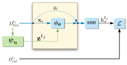
Figure 1: The ADKL algorithm. The green component corresponds to the adaptive part of the algorithm, which contrasts it with standard deep kernel learning approaches.

Task Encoding

One challenge for the network ${\boldsymbol{\psi}}_{{\boldsymbol{\eta}}}$ is to capture complex dependencies in the training set $D^{t}_{trn}$ to provide a useful task encoding ${\mathbf{z}}$. Furthermore, the task encoder should be invariant to permutations of the training set and be able to encode a variable amount of samples. After exploring a variety of architectures, we found that more complex ones such as Transformers [23] tend to underperform. This is possibly due to overfitting or the challenges associated with training such architectures.

Consequently, we introduce slight modifications to DeepSets, an order invariant network proposed by Zaheer et al. [16]. It begins with the computation of the representation of each input-target pair ${\mathbf{xy}}_{i}={\mathbf{r}}(\textit{Concat}({\mathbf{u}}({\mathbf{x}}_{i}),{\mathbf{v}}(y_{i})))$ for all $({\mathbf{x}}_{i},y_{i})\in D^{t}_{trn}$, using neural networks ${\mathbf{u}},{\mathbf{v}},\text{ and }{\mathbf{r}}$. This allows ${\mathbf{xy}}_{i}$ to capture nonlinear interactions between the inputs and the targets if ${\mathbf{r}}$ is a nonlinear transformation. Then, by computing the empirical mean $\mu^{t}_{{\mathbf{xy}}}$ and standard deviation $\sigma^{t}_{{\mathbf{xy}}}$ of the set $\left\{{\mathbf{xy}}_{1},{\mathbf{xy}}_{2},\ldots,{\mathbf{xy}}_{m}\right\}$, we obtain the task representation

$${\mathbf{z}}^{t}={\boldsymbol{\psi}}_{{\boldsymbol{\eta}}}(D^{t}_{trn}):={\mathbf{w}}(\textit{Concat}(\mu^{t}_{{\mathbf{xy}}},\sigma^{t}_{{\mathbf{xy}}})),$$ (10)

where ${\mathbf{w}}$ is a also a neural network. As $\mu^{t}_{{\mathbf{xy}}}$ and $\sigma^{t}_{{\mathbf{xy}}}$ are invariant to permutations in $D^{t}_{trn}$, it follows that ${\boldsymbol{\psi}}_{{\boldsymbol{\eta}}}$ is also permutation invariant. In summary, ${\boldsymbol{\psi}}_{{\boldsymbol{\eta}}}$ is a nonlinear mapping of the first and second moment of the sample representations which were also nonlinear transformations of the original inputs and targets. The learnable parameters ${\boldsymbol{\eta}}$ of the task encoder include all the parameters of the networks ${\mathbf{u}},{\mathbf{v}},{\mathbf{r}},\text{ and }{\mathbf{w}}$, and are shared across all tasks.

Adapted Kernel Computation

Once the task representation is obtained, we compute the conditional input embedding using the function ${\boldsymbol{\phi}}_{{\boldsymbol{\theta}}}$. Let ${\mathbf{u}}^{\prime}({\mathbf{x}})$ be the non-conditional embedding of the input ${\mathbf{x}}$ using a neural network ${\mathbf{u}}^{\prime}$, whose parameters are shared with the network ${\mathbf{u}}$ within the task encoder. We simply compute the conditional embedding of inputs as:

$${\boldsymbol{\phi}}_{{\boldsymbol{\theta}}}({\mathbf{x}};{\mathbf{z}}_{t})={\mathbf{o}}(\textit{Concat}({\mathbf{u}}^{\prime}({\mathbf{x}}),{\mathbf{z}}_{t})),$$ (11)

where ${\mathbf{o}}$ is a nonlinear neural network that allows for capturing complex interactions between the task and the input representations. The adapted kernel for a given task is then obtained by combining Equations 9, 10, 11. The learnable parameters of ${\mathbf{o}}$ and ${\mathbf{u}}^{\prime}$ together constitute ${\boldsymbol{\theta}}$ and are shared across all tasks. Alternatively, different architectures such as Feature-wise Linear Modulation (FiLM) [24], Hypernetwork [25], or Bilinear transformation [26] could be used to compute ${\boldsymbol{\phi}}_{{\boldsymbol{\theta}}}({\mathbf{x}};{\mathbf{z}})$, though we found that a simple concatenation was sufficient for our applications.

Kernel Methods

To find the regressor that minimizes Equation 1 for each task $t$, we use GP and KRR described in Section 2. In the following, we use ADKL-GP and ADKL-KRR to refer to our algorithm when the task-level regressor is given by GP and KRR, respectively.

3.2 Meta-Regularization

To assist in the training of the ADKL algorithm, we minimize a contrastive loss between $D^{t_{j}}_{trn}$ and $D^{t_{j}}_{val}$. Doing so, we encourage the encoder ${\boldsymbol{\psi}}_{{\boldsymbol{\eta}}}$ to embed datasets of the same task closer than those from different tasks. The non-parametric classification loss [27] and its variants, such as NT-Xent [28] and InfoNCE [29] are popular choices for the contrastive loss function, but herein we use the InfoNCE. Using a mini-batch approximation of the expectations, this yields the regularizer $\tilde{I}_{{\boldsymbol{\eta}}}$ defined as follows:

$$\tilde{I}_{{\boldsymbol{\eta}}}\overset{{\rm\mbox{\tiny def}}}{=}\tfrac{1}{b}\sum_{j=1}^{b}{\boldsymbol{\psi}}_{{\boldsymbol{\eta}}}(D^{t_{j}}_{trn})\cdot{\boldsymbol{\psi}}_{{\boldsymbol{\eta}}}(D^{t_{j}}_{val})-\ln\tfrac{1}{b(b-1)}\sum_{j=1}^{b}\sum_{i\neq j}e^{{\boldsymbol{\psi}}_{{\boldsymbol{\eta}}}(D^{t_{j}}_{trn})\cdot{\boldsymbol{\psi}}_{{\boldsymbol{\eta}}}(D^{t_{i}}_{val})}.$$ (12)

When adding this to our training objective with $\gamma\geq 0$ as a tradeoff hyperparameter, we have:

$$\underset{{\boldsymbol{\theta}},{\boldsymbol{\eta}},{\boldsymbol{\rho}},\lambda}{\mathrm{argmin}}\ \underset{t_{j}\sim B}{\mathrm{{\mathbf{E}}}}\ {\mathcal{L}}_{{\boldsymbol{\theta}},{\boldsymbol{\eta}},{\boldsymbol{\rho}},\lambda}^{t_{j}}-\gamma\tilde{I}_{{\boldsymbol{\eta}}}.$$ (13)

4 Related Work

Our study spans the research areas of deep kernel learning and few-shot learning. For a comprehensive overview of few-shot learning methods, we refer the reader to Wang and Yao [1], Chen et al. [2], as we focus on work related to DKL herein.

Across the spectrum of learning approaches, DKL methods lie between neural networks and kernel methods. While neural networks can learn from a very large amount of data without much prior knowledge, kernel methods learn from fewer data when given an appropriate covariance function that accounts for prior knowledge of the task at hand. In the first DKL attempt, Wilson et al. [19] combined GP with CNN to learn a covariance function adapted to a task from large amounts of data, though the large time and space complexity of kernel methods forced the approximation of the exact kernel using KISS-GP [22]. Dasgupta et al. [30] have demonstrated that such approximation is not necessary using finite rank kernels. Here, we also show that learning from a collection of tasks (FSR mode) does not require any approximation when the covariance function is shared across tasks. This is an important distinction between our study and other existing studies in DKL, which learn their kernel from single tasks instead of task collections.

On the spectrum between NNs and kernel methods, metric learning also bears mention. Metric learning algorithms learn an input covariance function shared across tasks but rely only on the expressive power of DNNs. First, stochastic kernels are built out of shared feature extractors, simple pairwise metrics (e.g. cosine similarity [9], Euclidean distance [10]), or parametric functions (e.g. relation modules [31], graph neural networks [11]). Then, within tasks, the predictions consist of a distance-weighted combination of the training sample labels with the stochastic kernel evaluations—no adaptation is done. The recently introduced Proto-MAML [13] method, which captures the best of Prototypical Networks [10] and MAML [14], allows within-task adaptation using MAML on a network built on top of the kernel function. Similarly, Kim et al. [6] have proposed a Bayesian version of MAML where a feature extractor is shared across tasks, while multiple MAML particles are used for the task-level adaptation. Bertinetto et al. [12] have also tackled this lack of adaptation for new tasks by using KRR and Logistic Regression to find the appropriate weighting of the training samples. This study can be considered the first application of DKL to few-shot learning. However, its contribution was limited to showing that simple differentiable learning algorithms can increase adaptation in the metric learning framework. Our work extends beyond by formalizing few-shot learning in the deep kernel learning framework where test-time adaptation is achieved through kernel methods. We also create another layer of adaptation by allowing task-specific kernels that are created at test-time.

Since ADKL-GP uses GPs, it is related to neural processes [32], which proposes a scalable alternative to learning regression functions by performing inference on stochastic processes. Furthermore, in this family of methods, Conditional Neural Processes (CNP) [33] and Attentive Neural Processes (ANP) [34] are even more relevant to our study as both methods learn conditional stochastic processes parameterized by conditions derived from training data points. While ANP imposes consistency with respect to some prior process, CNP does not and thus does not have the mathematical guarantees associated with stochastic processes. By comparison, our proposed ADKL-GP algorithm also learns conditional stochastic processes, but within the GP framework, thus benefiting from the associated mathematical guarantees.

5 Experiments

5.1 Datasets

Previous work on few-shot regression has relied on synthetic datasets to evaluate performance. We instead introduce two real-world benchmarks drawn from the field of drug discovery. These benchmarks will allow us to measure the ability of few-shot learning algorithms to adapt in settings where tasks require a considerably different measure of similarity between the inputs. For instance, when predicting binding affinities between small molecules, the covariance function must learn characteristics of a protein binding site that changes between proteins or tasks. We describe each dataset used in our experiments below and, unless stated otherwise, the meta-training, meta-validation, and meta-testing contain, respectively, 56.25%, 18.75% and 25% of all of their tasks. A pre-processed version of these datasets is available with this work here

1. Sinusoids: This meta-dataset was recently proposed by Kim et al. [6] as a challenging few-shot synthetic regression benchmark. It consists of 5,000 tasks defined by a sinusoidal functions of the form: $y~{}=~{}A~{}\sin(wx~{}+~{}b)~{}+~{}\epsilon$. The parameters $A,w,b$ characterize each task and are drawn from the following intervals: $A\in\left[0.1,5.0\right]$, $b\in\left[0.0,2\pi\right]$, $w\in\left[0.5,2.0\right]$. Samples for each task are generated by sampling inputs $x\in[-5.0,5.0]$ and observational noise from $\epsilon\sim N(0,(0.01A)^{2})$. Every model on this task collection uses a fully connected network of 2 layers of 120 hidden units as its input feature extractor. Visuals of ground truths and predictions for some functions are shown in Appendix C:.

2. Binding: The goal here is to predict the binding affinity of small, drug-like molecules to proteins. This task collection was extracted from the public database BindingDB and encompasses 7,620 tasks, each containing between 7 and 9,000 samples. Each task corresponds to a protein sequence, which thus defines a separate distribution on the input space of molecules and the output space of (real-valued) binding readouts.

3. Antibacterial: The goal here is to predict the antimicrobial activity of small molecules for various bacteria. The task collection was extracted from the public database PubChem and contains 3,842 tasks, each consisting of 5 to 225 samples. A task corresponds to a combination of a bacterial strain and an experimental setting, which define different data distributions.

For both real-world datasets, the molecules are represented by their SMILES encoding, which are descriptions of the molecular structure using short ASCII strings. All models evaluated on these collections share the same input feature extractor configuration: a 1-D CNN of 2 layers of 128 hidden units each and a kernel size of  5. We choose CNN instead of LSTM or advanced graph convolutions methods for scalability reasons. Finally, all targets were scaled linearly between 0 and 1.

5.2 Benchmarking analysis

We evaluate model performance against R2-D2 [12], CNP[33], and MAML[14]. Comparing R2-D2 to ADKL-KRR when using the linear kernel allows us to determine whether the adapted deep kernel provides improved test-time adaptation. CNP is also a relevant comparison to ADKL-GP and allows us to measure performance differences between the task-level Bayesian models generated within the GP and CNP frameworks. MAML is considered herein for its fast-adaptation at test-time and as the representative of initialization and optimization based methods. In the following experiments, all DKL methods use the linear kernel.

Our first set of experiments evaluates performance on both the real-world and toy tasks. We train each method using support and query sets of size $m~{}=~{}10$. During meta-testing, the support set size is also $m~{}=~{}10$, but the query set consists of the remaining samples of each task. For the datasets lacking sufficient samples such as in the Binding and Antibacterial collections, we use half of the samples in the support set and the remaining in the query set. During meta-testing of each task, we average the Mean Squared Error (MSE) over 20 random partitions of the query and support sets. We refer to this value as the task MSE. Figure 2 illustrates the task MSE distributions over tasks for each collection and algorithm (best hyperparameters were chosen on the meta-validation set). In general, we observe that the real-world datasets are challenging for all methods but ADKL methods consistently outperform R2-D2 and CNP. The MSE difference between ADKL-KRR and R2-D2 support the importance of adapting the kernel to each task rather than sharing a single kernel. Furthermore, we observe that ADKL-GP outperforms CNP, showing the effectiveness of the ADKL approach in comparison with conditional neural processes. Finally, both adaptive deep kernel methods (ADKL-KRR and ADKL-GP) seem to perform comparably, despite different objective functions.

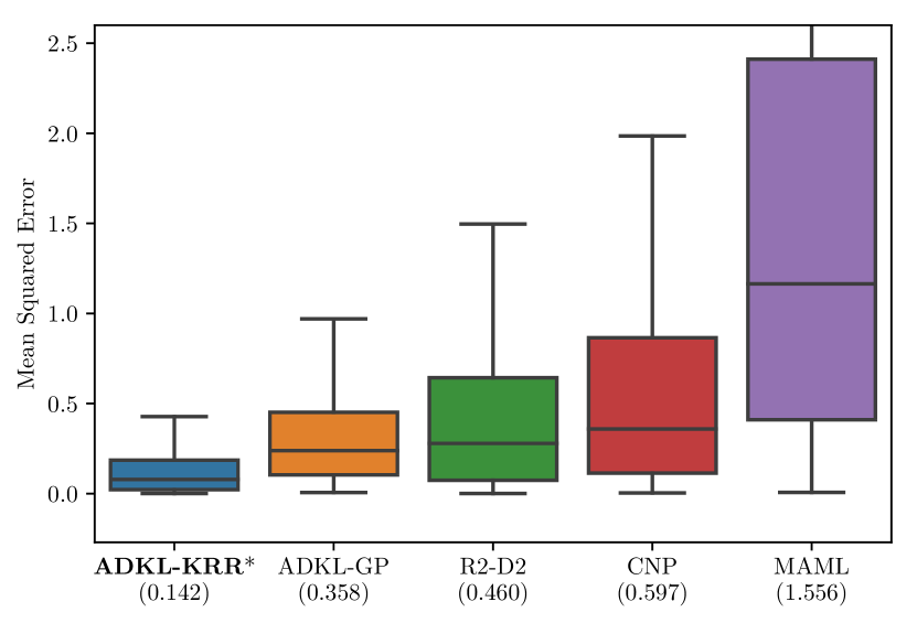
(a) Sinusoids collection

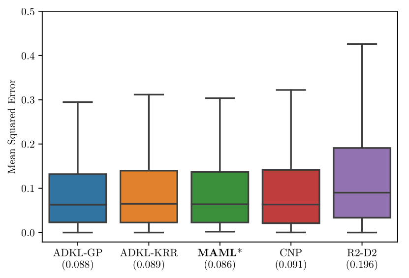
(b) Binding collection

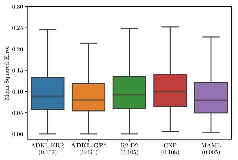
(c) Antibacterial collection

Figure 2: MSE distributions for tasks in the meta-testing sets. Only the best model for each dataset is marked with an asterisk and the mean MSE for the whole meta-test is shown below the algorithm name.

A second experimental set is used to measure the across-task generalization and within-task adaptation capabilities of the different methods. We do so by controlling the number of training tasks ($T\in\left\{100,1000\right\}$) and the size of the support sets ($m\in\left\{5,10,15,20,25,30\right\}$) during meta-training and meta-testing. Only the Sinusoids collection was used, as experiments with the real-world collections were deemed too time-consuming for the scope of this study. One would expect the algorithms to generalize poorly to new tasks for lower values of $T$, and their task-level models to adapt poorly to new samples for small values of $m$. However, as illustrated in Figure 3, all DKL methods generalize better across tasks than other algorithms. DKL methods also demonstrate improved within-task generalization using as few as 15 samples, while other methods require more samples to achieve similar MSE. Moreover, for small support sets, ADKL-KRR shows better within-task generalization than ADKL-GP and R2-D2. The difference in performance between ADKL-KRR and R2-D2 can be attributed to the kernel adaptation at test-time as this is the only difference between both methods. When $m$ is small, the difference between ADKL-GP and ADKL-KRR can be attributed to larger predictive uncertainty in GP as the number of samples gets smaller.

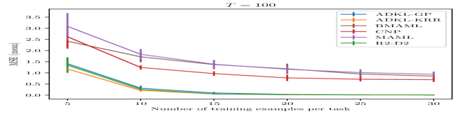
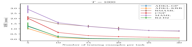
Figure 3: Average MSE over the testing tasks of the Sinusoids collection. The error bars represent the uncertainty on the average over 5 runs with different seeds.

5.3 Active Learning

What follows aims to measure the effectiveness of the uncertainty captured by the predictive distribution of ADKL-GP for active learning. By comparing to CNP, we’ll quantify which of CNP or GP better captures the data uncertainty for improving FSR under active sample selection. For this purpose, we meta-train both algorithms using support and query sets of size $m~{}=~{}5$ and use $T\in\left\{100,1000\right\}$ for the Sinusoids collection. During meta-test time, five samples are randomly selected to constitute the support set $D_{trn}$ and build the initial hypothesis for each task. Then, from a pool $U$ of unlabeled data, we choose the input ${\mathbf{x}}^{*}$ of maximum predictive entropy, i.e., ${\mathbf{x}}^{*}=\mathrm{argmax}_{{\mathbf{x}}\in U}{\mathbb{E}\left[\log p(y\lvert{\mathbf{x}},D_{trn})\right]}$. The latter example is removed from $U$ and added to $D_{trn}$ with its predicted label. The within-task adaptation is performed on the new support set to obtain a new hypothesis which is evaluated on the query set $D_{val}$ of the task. This process is repeated until we reach the allowed budget of $20$ queries.

Figure 4 highlights that, in the active learning setting, ADKL-GP consistently outperforms CNP. Very few samples are queried by ADKL-GP to appropriately capture the data distribution. In contrast, CNP performance is far from optimal, even when allowed the maximum number of queries. Also, since using the maximum predictive entropy strategy is better than querying samples at random for ADKL-GP (solid vs. dashed line), these results suggest that the predictive uncertainty obtained with GP is more informative and accurate than that of CNP. Moreover, when the number of queries is greater than $10$, we observe a performance degradation for CNP, while ADKL-GP remains consistent. This observation highlights the generalization capacity of DKL methods, even outside the few-shot regime where they have been trained. We attribute this property of DKL methods to their use of kernel methods.

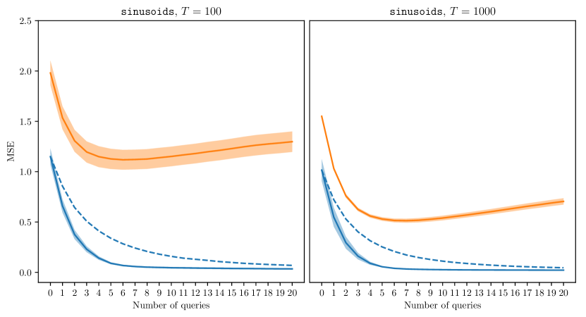
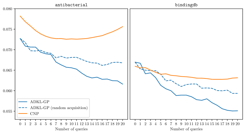
Figure 4: Average MSE performance on the meta-test during active learning. The width of the shaded regions denotes the uncertainty over five runs for the sinusoidal collection. No uncertainty is shown for the real-world tasks as they were too time consuming.

5.4 Impact of Regularization and Kernel

In our final set of experiments, we take a closer look at the impact of the base kernel and the meta-regularization factor on the generalization during meta-testing. We do so by evaluating ADKL-KRR on the Sinusoids collection with different hyperparameter combinations. Figure 5 (left) shows the performances obtained by varying the meta-regularization parameter $\gamma$ over different hyperparameter configurations (listed in Appendix A:). When looking at values of $\gamma\in\left\{0,0.1,0.01\right\}$, we observe that non-zero values help in most cases, meaning that the added regularizer improves slightly the task encoder learning. As choosing the appropriate kernel function is crucial for kernel methods, we also measure how different base kernels impact the learning process. To do so, we test the linear and RBF kernels, and their normalized versions as given by $k^{\prime}({\mathbf{x}},{\mathbf{x}}^{\prime}):={k({\mathbf{x}},{\mathbf{x}}^{\prime})}/{\sqrt{k({\mathbf{x}},{\mathbf{x}})k({\mathbf{x}}^{\prime},{\mathbf{x}}^{\prime})}}$. Over different hyperparameter combinations, we observe that the linear kernel yields better generalization performances than the RBF kernel (see Figure 5 right). Such a result is within expectation as the scaling parameter of the RBF kernel is shared across tasks, making it more difficult to adapt the deep kernel. In future work, it would be interesting to explore learning the base kernel hyperparameters using a network similar to ${\boldsymbol{\psi}}$.

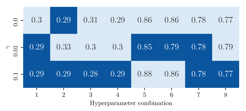
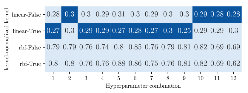
Figure 5: Impact of $\gamma$ and the kernel on the average meta-test MSE for different hyperparameter combinations (dark blue is best). The combinations are detailed in the Appendix B: and Appendix A:

6 Conclusion

In this paper, we investigated the benefits of deep kernel learning (DKL) methods for few-shot regression (FSR). By comparing methods on real-world and synthetic task collections, we successfully demonstrated the effectiveness of the DKL framework in FSR. Both ADKL-GP and ADKL-KRR outperform the single kernel DKL method, providing evidence of their improved adaptation capacity at test-time through adaptation of the kernel. Given the Bayesian nature of ADKL-GP, this variation of the main algorithm allows for improvement of the learned models at test-time, providing unique opportunities in settings such as drug discovery where active learning can be deployed in design-make-test cycles. Finally, by making our drug discovery task collections publicly available, we hope to encourage the machine learning community to work toward new FSR algorithms that can be better adapted to real-world drug-discovery settings.

Appendix Appendix A: Regularization impact

Table 1 presents the hyperparameter combinations used in the experiments to assess the impact of the joint training parameter $\gamma$.

Table 1: Effect of using joint training (parameter $\gamma$) on the MSE performances

			$\gamma$	0.0	0.01	0.1
Run	kernel	hidden size (target FE)	hidden size (input FE)
1	linear	[32, 32]	[128, 128, 128]	0.297	0.290	0.290
2	linear	[32, 32]	[128, 128]	0.288	0.328	0.288
3	linear	[]	[128, 128, 128]	0.306	0.300	0.285
4	linear	[]	[128, 128]	0.290	0.297	0.287
5	rbf	[32, 32]	[128, 128, 128]	0.864	0.851	0.876
6	rbf	[32, 32]	[128, 128]	0.859	0.787	0.864
7	rbf	[]	[128, 128, 128]	0.780	0.778	0.778
8	rbf	[]	[128, 128]	0.769	0.793	0.768

Note that the performance is significantly worse when using RBF kernel.

Appendix Appendix B: Kernel impact

Table 2 shows the hyperparameter combinations we used to assess the effect of using different kernels, as well as the impact of normalizing them.

Table 2: MSE performance depending on the kernel choice and normalization

			kernel	Linear		RBF
			normalized	False	True	False	True
Run	encoder arch	target FE	input FE
1	CNP	[32, 32]	[128, 128, 128]	0.279	0.274	0.786	0.795
2	CNP	[32, 32]	[128, 128]	0.299	0.300	0.789	0.799
3	CNP	[]	[128, 128, 128]	0.304	0.289	0.761	0.755
4	CNP	[]	[128, 128]	0.295	0.293	0.742	0.757
5	DeepSet	[32, 32]	[128, 128, 128]	0.313	0.269	0.804	0.877
6	DeepSet	[32, 32]	[128, 128]	0.301	0.277	0.849	0.856
7	DeepSet	[]	[128, 128, 128]	0.292	0.273	0.764	0.754
8	DeepSet	[]	[128, 128]	0.303	0.298	0.788	0.763
9	KRR	[32, 32]	[128, 128, 128]	0.296	0.246	0.815	0.815
10	KRR	[32, 32]	[128, 128]	0.289	0.290	0.824	0.824
11	KRR	[]	[128, 128, 128]	0.279	0.291	0.690	0.694
12	KRR	[]	[128, 128]	0.275	0.299	0.685	0.622

Appendix Appendix C: Prediction curves on the Sinusoids collection

Figure 6 presents a visualization of the results obtained by each model on three tasks taken from the meta-test set. We provide the model with ten examples from an unseen task consisting of a slightly noisy sine function (shown in blue), and present in orange the the approximation made by the network based on these ten examples.

Note that contrary to others, CNP and ADKL-GP give us access to the uncertainty.

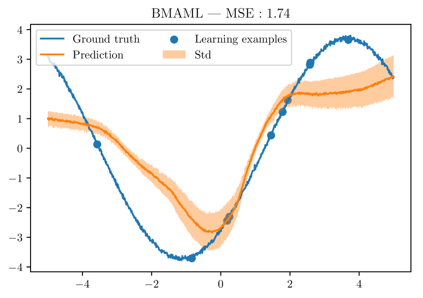
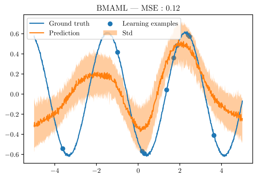
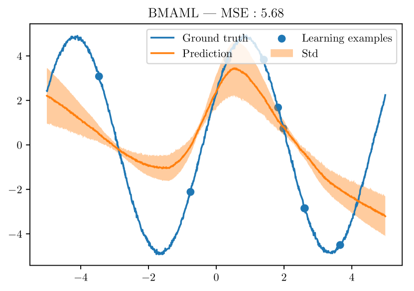
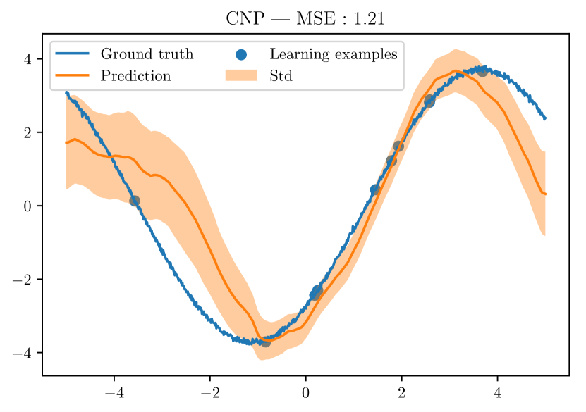
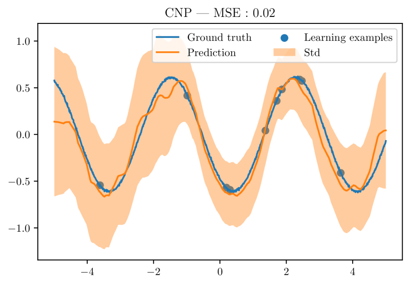
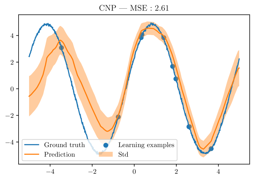
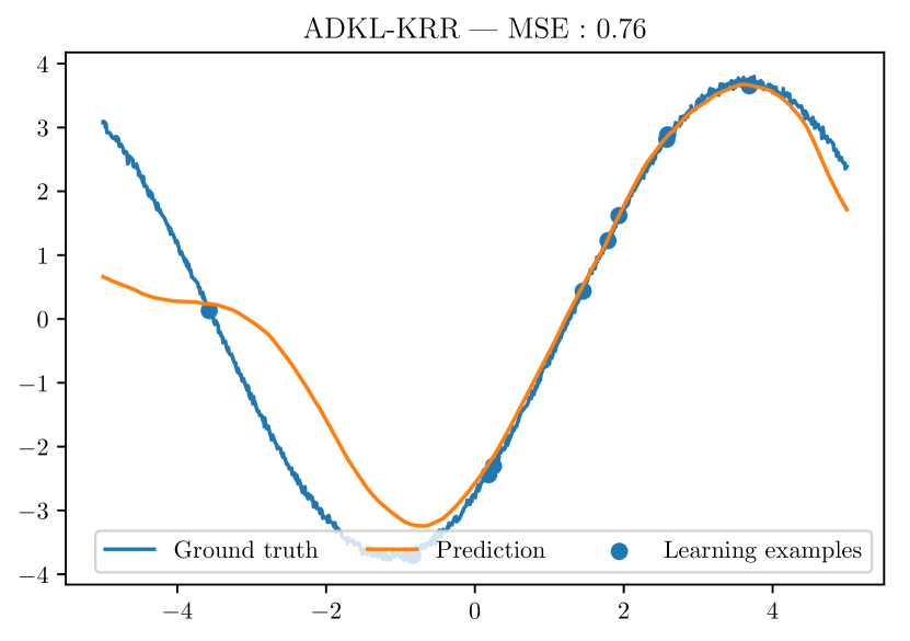
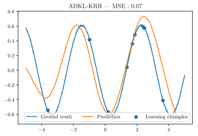
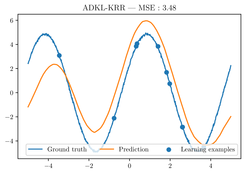
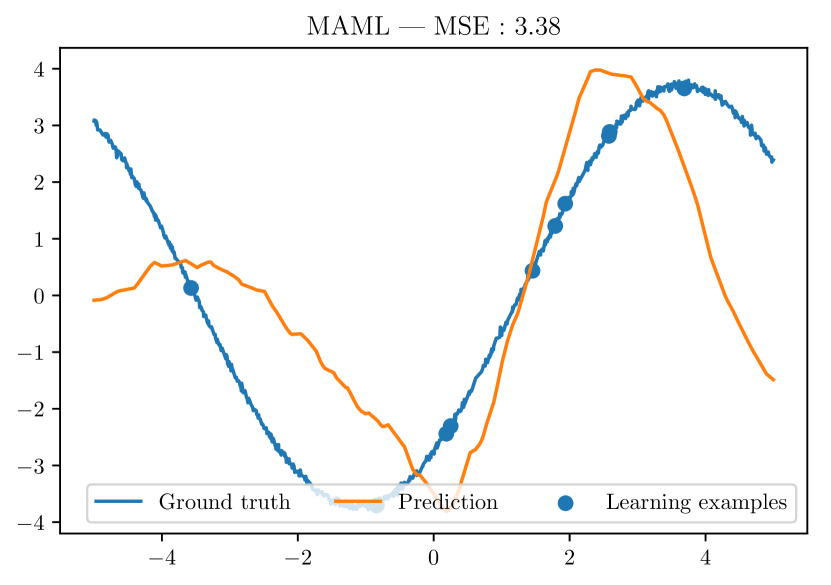
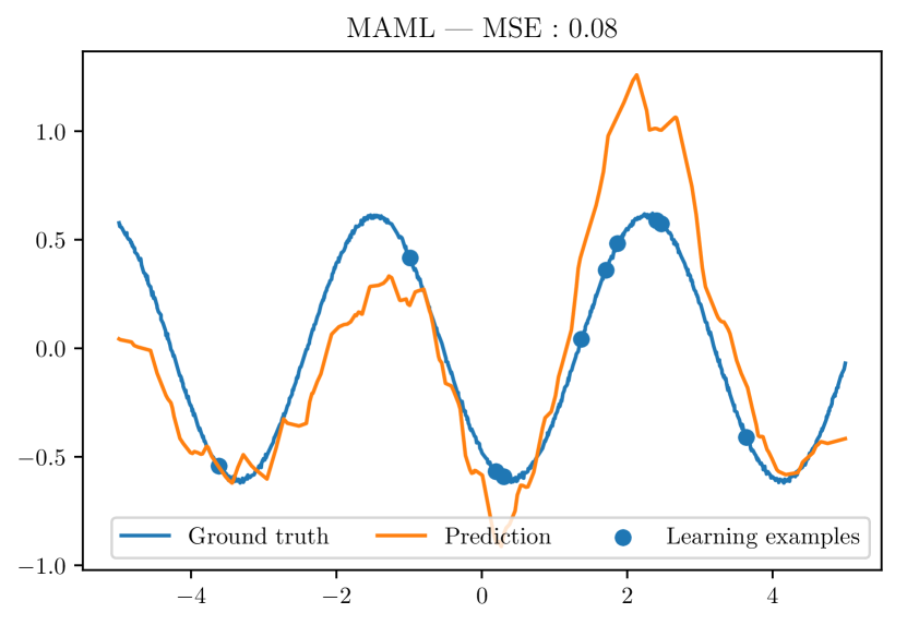
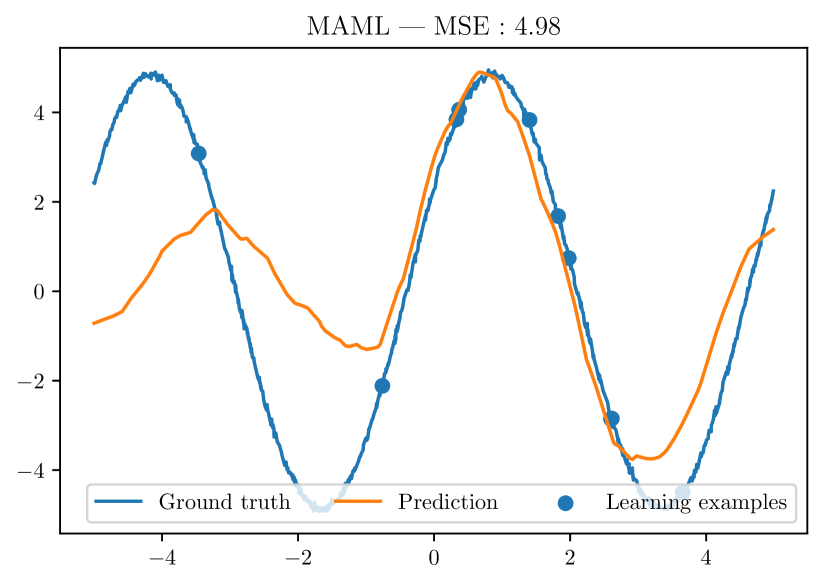
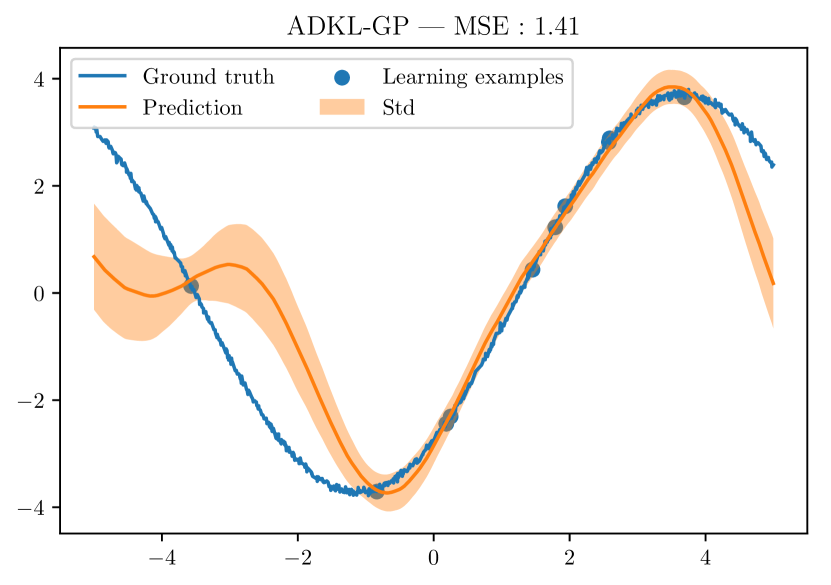
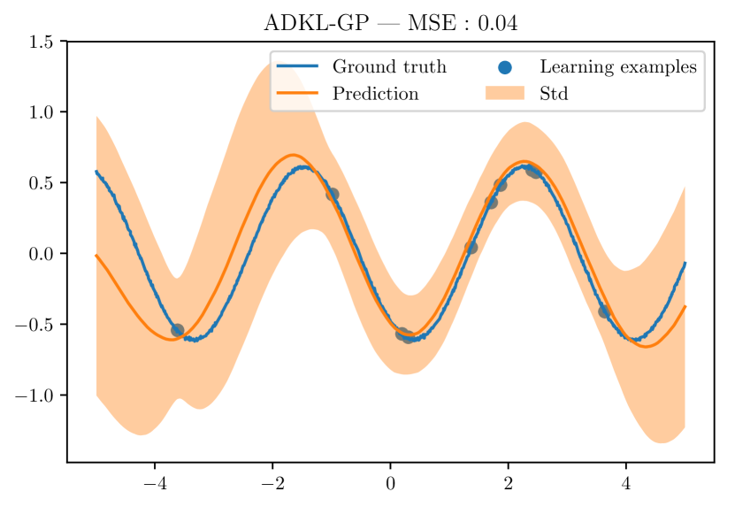
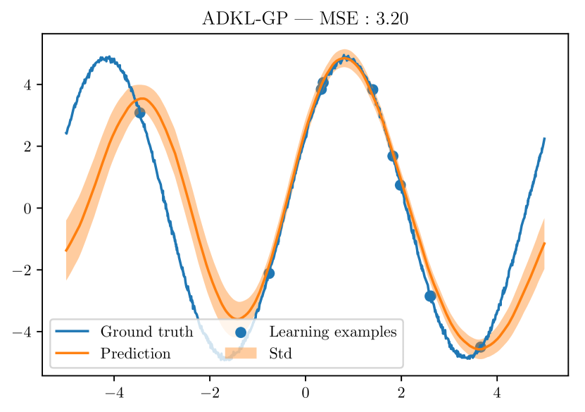
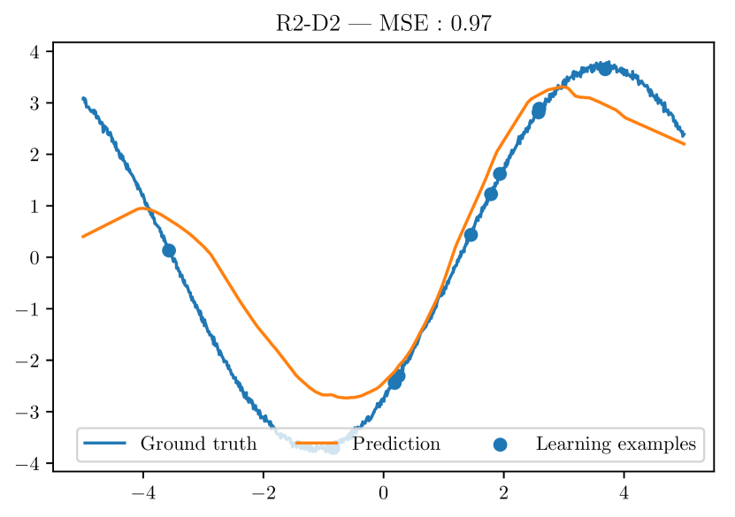
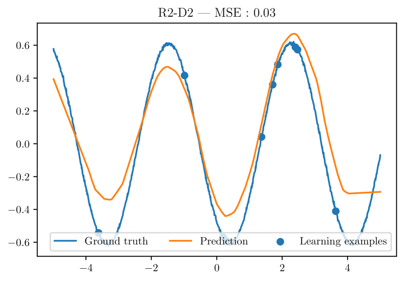
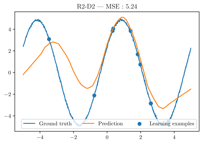
Figure 6: Meta-test time predictions on the Sinusoids collection

References

- Wang and Yao [2019] Yaqing Wang and Quanming Yao. Few-shot learning: A survey. CoRR, abs/1904.05046, 2019. URL http://arxiv.org/abs/1904.05046.
- Chen et al. [2019] Wei-Yu Chen, Yen-Cheng Liu, Zsolt Kira, Yu-Chiang Frank Wang, and Jia-Bin Huang. A closer look at few-shot classification. arXiv preprint arXiv:1904.04232, 2019.
- Thrun and Pratt [1998] Sebastian Thrun and Lorien Pratt. Learning to learn: Introduction and overview. In Learning to learn, pages 3–17. Springer, 1998.
- Vilalta and Drissi [2002] Ricardo Vilalta and Youssef Drissi. A perspective view and survey of meta-learning. Artificial intelligence review, 18(2):77–95, 2002.
- Li et al. [2017] Zhenguo Li, Fengwei Zhou, Fei Chen, and Hang Li. Meta-sgd: Learning to learn quickly for few-shot learning. arXiv preprint arXiv:1707.09835, 2017.
- Kim et al. [2018] Taesup Kim, Jaesik Yoon, Ousmane Dia, Sungwoong Kim, Yoshua Bengio, and Sungjin Ahn. Bayesian model-agnostic meta-learning. arXiv preprint arXiv:1806.03836, 2018.
- Loo et al. [2019] Yi Loo, Swee Kiat Lim, Gemma Roig, and Ngai-Man Cheung. Few-shot regression via learned basis functions. open review preprint:r1ldYi9rOV, 2019.
- Koch et al. [2015] Gregory Koch, Richard Zemel, and Ruslan Salakhutdinov. Siamese neural networks for one-shot image recognition. In ICML deep learning workshop, volume 2, 2015.
- Vinyals et al. [2016] Oriol Vinyals, Charles Blundell, Timothy Lillicrap, Daan Wierstra, et al. Matching networks for one shot learning. In Advances in neural information processing systems, pages 3630–3638, 2016.
- Snell et al. [2017] Jake Snell, Kevin Swersky, and Richard Zemel. Prototypical networks for few-shot learning. In Advances in Neural Information Processing Systems, pages 4077–4087, 2017.
- Garcia and Bruna [2017] Victor Garcia and Joan Bruna. Few-shot learning with graph neural networks. arXiv preprint arXiv:1711.04043, 2017.
- Bertinetto et al. [2018] Luca Bertinetto, Joao F Henriques, Philip HS Torr, and Andrea Vedaldi. Meta-learning with differentiable closed-form solvers. arXiv preprint arXiv:1805.08136, 2018.
- Triantafillou et al. [2019] Eleni Triantafillou, Tyler Zhu, Vincent Dumoulin, Pascal Lamblin, Kelvin Xu, Ross Goroshin, Carles Gelada, Kevin Swersky, Pierre-Antoine Manzagol, and Hugo Larochelle. Meta-dataset: A dataset of datasets for learning to learn from few examples. arXiv preprint arXiv:1903.03096, 2019.
- Finn et al. [2017] Chelsea Finn, Pieter Abbeel, and Sergey Levine. Model-agnostic meta-learning for fast adaptation of deep networks. In Proceedings of the 34th International Conference on Machine Learning-Volume 70, pages 1126–1135. JMLR. org, 2017.
- Ravi and Larochelle [2016] Sachin Ravi and Hugo Larochelle. Optimization as a model for few-shot learning. 2016.
- Zaheer et al. [2017] Manzil Zaheer, Satwik Kottur, Siamak Ravanbakhsh, Barnabas Poczos, Ruslan R Salakhutdinov, and Alexander J Smola. Deep sets. In Advances in neural information processing systems, pages 3391–3401, 2017.
- Scholkopf and Smola [2001] Bernhard Scholkopf and Alexander J Smola. Learning with kernels: support vector machines, regularization, optimization, and beyond. MIT press, 2001.
- Williams and Rasmussen [1996] Christopher KI Williams and Carl Edward Rasmussen. Gaussian processes for regression. In Advances in neural information processing systems, pages 514–520, 1996.
- Wilson et al. [2016] Andrew Gordon Wilson, Zhiting Hu, Ruslan Salakhutdinov, and Eric P Xing. Deep kernel learning. In Artificial Intelligence and Statistics, pages 370–378, 2016.
- Steinwart and Christmann [2008] Ingo Steinwart and Andreas Christmann. Support vector machines. Springer Science & Business Media, 2008.
- Williams and Seeger [2001] Christopher KI Williams and Matthias Seeger. Using the nyström method to speed up kernel machines. In Advances in neural information processing systems, pages 682–688, 2001.
- Wilson and Nickisch [2015] Andrew Wilson and Hannes Nickisch. Kernel interpolation for scalable structured gaussian processes (kiss-gp). In International Conference on Machine Learning, pages 1775–1784, 2015.
- Vaswani et al. [2017] Ashish Vaswani, Noam Shazeer, Niki Parmar, Jakob Uszkoreit, Llion Jones, Aidan N Gomez, Łukasz Kaiser, and Illia Polosukhin. Attention is all you need. In Advances in neural information processing systems, pages 5998–6008, 2017.
- Perez et al. [2018] Ethan Perez, Florian Strub, Harm De Vries, Vincent Dumoulin, and Aaron Courville. Film: Visual reasoning with a general conditioning layer. In Thirty-Second AAAI Conference on Artificial Intelligence, 2018.
- Ha et al. [2016] David Ha, Andrew Dai, and Quoc V Le. Hypernetworks. arXiv preprint arXiv:1609.09106, 2016.
- Tenenbaum and Freeman [2000] Joshua B Tenenbaum and William T Freeman. Separating style and content with bilinear models. Neural computation, 12(6):1247–1283, 2000.
- Wu et al. [2018] Zhirong Wu, Yuanjun Xiong, Stella Yu, and Dahua Lin. Unsupervised feature learning via non-parametric instance-level discrimination, 2018.
- Chen et al. [2020] Ting Chen, Simon Kornblith, Mohammad Norouzi, and Geoffrey Hinton. A simple framework for contrastive learning of visual representations, 2020.
- van den Oord et al. [2019] Aaron van den Oord, Yazhe Li, and Oriol Vinyals. Representation learning with contrastive predictive coding, 2019.
- [30] Sambarta Dasgupta, Kumar Sricharan, and Ashok Srivastava. Finite rank deep kernel learning.
- Sung et al. [2018] Flood Sung, Yongxin Yang, Li Zhang, Tao Xiang, Philip HS Torr, and Timothy M Hospedales. Learning to compare: Relation network for few-shot learning. In Proceedings of the IEEE Conference on Computer Vision and Pattern Recognition, pages 1199–1208, 2018.
- Garnelo et al. [2018a] Marta Garnelo, Jonathan Schwarz, Dan Rosenbaum, Fabio Viola, Danilo J Rezende, SM Eslami, and Yee Whye Teh. Neural processes. arXiv preprint arXiv:1807.01622, 2018a.
- Garnelo et al. [2018b] Marta Garnelo, Dan Rosenbaum, Chris J Maddison, Tiago Ramalho, David Saxton, Murray Shanahan, Yee Whye Teh, Danilo J Rezende, and SM Eslami. Conditional neural processes. arXiv preprint arXiv:1807.01613, 2018b.
- Kim et al. [2019] Hyunjik Kim, Andriy Mnih, Jonathan Schwarz, Marta Garnelo, Ali Eslami, Dan Rosenbaum, Oriol Vinyals, and Yee Whye Teh. Attentive neural processes. arXiv preprint arXiv:1901.05761, 2019.