Classification of Real Solutions of the Fourth Painlevé Equation

Abstract

Painlevé transcendents are usually considered as complex functions of a complex variable, but in applications it is often the real cases that are of interest. Under a reasonable assumption (concerning the behavior of a dynamical system associated with Painlevé IV, as discussed in a recent paper), we give a number of results towards a classification of the real solutions of Painlevé IV (or, more precisely, symmetric Painlevé IV), according to their asymptotic behavior and singularities. We show the existence of globally nonsingular real solutions of symmetric Painlevé IV for arbitrary nonzero values of the parameters, with the dimension of the space of such solutions and their asymptotics depending on the signs of the parameters. We show that for a generic choice of the parameters, there exists a unique finite sequence of singularities for which symmetric Painlevé IV has a two-parameter family of solutions with this singularity sequence. There also exist solutions with singly infinite and doubly infinite sequences of singularities, and we identify which such sequences are possible (assuming generic asymptotics in the case of a singly infinite sequence). Most (but not all) of the special solutions of Painlevé IV correspond to nongeneric values of the parameters, but we mention some results for these solutions as well.

1 Introduction and Contents of This Paper

The six Painlevé equations were initially discovered in the context of the classification of second order ordinary differential equations with the property that the only movable singularities of their solutions are poles. In this context solutions of the Painlevé equations are naturally considered as complex functions of a complex variable. Since their initial discovery, however, many applications of Painlevé equations have emerged (see [8, 11] for a comprehensive list). In many of these applications, the relevant solutions are real functions of a real variable. It is therefore of interest to have a classification of real solutions. In a recent paper [19] we described a dynamical systems approach to the fourth Painlevé equation ($P_{\mathrm{IV}}$). In the current paper we use this approach to develop a qualitative classification of the real solutions of $P_{\mathrm{IV}}$ for suitable parameter values.

In fact we work with $sP_{\mathrm{IV}}$, the symmetric version of $P_{\mathrm{IV}}$. Recall that $P_{\mathrm{IV}}$ is the equation

$$\frac{{\mathrm{d}}^{2}w}{{\mathrm{d}z}^{2}}=\frac{1}{2w}\left(\frac{\mathrm{d}w}{\mathrm{d}z}\right)^{2}+\frac{3}{2}w^{3}+4zw^{2}+2(z^{2}-\alpha)w+\frac{\beta}{w},$$ (1)

with two parameters, $\alpha$ and $\beta$ (we take $\beta\leq 0$). $sP_{\mathrm{IV}}$ is the three-dimensional system

$$\frac{\mathrm{d}f_{1}}{\mathrm{d}x} =f_{1}(f_{2}-f_{3})+\alpha_{1}\ ,$$ (2a)

$$\frac{\mathrm{d}f_{2}}{\mathrm{d}x} =f_{2}(f_{3}-f_{1})+\alpha_{2}\ ,$$ (2b)

$$\frac{\mathrm{d}f_{3}}{\mathrm{d}x} =f_{3}(f_{1}-f_{2})+\alpha_{3}\ ,$$ (2c)

subject to

$$\alpha_{1}+\alpha_{2}+\alpha_{3}=1\ ,$$ (3)

and

$$f_{1}+f_{2}+f_{3}=x\ .$$ (4)

$sP_{\mathrm{IV}}$ was known to Bureau [4] but was rediscovered by Adler [1] and Noumi and Yamada [15, 16], amongst others. The relationship between $P_{\mathrm{IV}}$ and $sP_{\mathrm{IV}}$ is a little subtle: If $f_{1},f_{2},f_{3}$ is a solution of (2)–(4) and we set $w(z)=-\sqrt{2}f_{1}(x)$, where $z=\frac{x}{\sqrt{2}}$, then $w(z)$ is a solution of (1) with parameter values $\alpha=\alpha_{3}-\alpha_{2}$ and $\beta=-2\alpha_{1}^{2}$. But also, by the evident cyclic symmetry of $sP_{\mathrm{IV}}$, if we set $w(z)=-\sqrt{2}f_{2}(x)$, then $w(z)$ is a solution of (1) with parameter values $\alpha=\alpha_{1}-\alpha_{3}$ and $\beta=-2\alpha_{2}^{2}$, and if we set $w(z)=-\sqrt{2}f_{3}(x)$, then $w(z)$ is a solution of (1) with parameter values $\alpha=\alpha_{2}-\alpha_{1}$ and $\beta=-2\alpha_{3}^{2}$. Thus the three components of a solution of the $sP_{\mathrm{IV}}$ system generically give three distinct solutions of $P_{\mathrm{IV}}$, with different parameter values. Going the other way (i.e. using a solution of $P_{\mathrm{IV}}$ to find a solution of $sP_{\mathrm{IV}}$) is more involved, as if $\beta=-2\alpha_{1}^{2}$ then $\alpha_{1}=\pm\sqrt{-\frac{\beta}{2}}$, so each of the maps from a solution of $sP_{\mathrm{IV}}$ to a solution of $P_{\mathrm{IV}}$ can be inverted in two different ways. These ambiguities give rise to some of the symmetries or Bäcklund transformations of $P_{\mathrm{IV}}$ and $sP_{\mathrm{IV}}$ [9]; we will describe these more succinctly in Section 2. From here on we work with $sP_{\mathrm{IV}}$ throughout; all results can be translated to equivalent results for $P_{\mathrm{IV}}$ with $\beta\leq 0$, but these are less elegant.

The parameters of $sP_{\mathrm{IV}}$ are $\alpha_{1},\alpha_{2},\alpha_{3}$ satisfying (3). If we introduce $\xi,\eta$ via

$$\alpha_{1} = \frac{1}{3}+\xi\ ,$$ (5)

$$\alpha_{2} = \frac{1}{3}-\frac{1}{2}\xi+\frac{\sqrt{3}}{2}\eta\ ,$$ (6)

$$\alpha_{3} = \frac{1}{3}-\frac{1}{2}\xi-\frac{\sqrt{3}}{2}\eta\ ,$$ (7)

then a set of parameters corresponds to a point on the $(\xi,\eta)$ plane. The lines on which one of $\alpha_{1},\alpha_{2},\alpha_{3}$ is an integer form a triangular lattice on this plane, see Figure 1. By generic parameter values we mean any value of the parameters for which all the $\alpha_{i}$ are noninteger. For values of the parameters corresponding to the vertices of the lattice or the centers of the cells of the lattice (marked, respectively, by black and white circles in Figure 1), there exist rational solutions, see [9]. For other nongeneric values of the parameters, solutions are known in terms of special functions [9]. Section 5 of this paper will be devoted to special solutions; apart from this, the focus of this paper is on generic parameter values.

Figure 1: The plane $\alpha_{1}+\alpha_{2}+\alpha_{3}=1$ viewed from the positive normal direction, with lines drawn where one of the $\alpha_{i}$ is integral. The lines on which one the $\alpha_{i}$ vanish are marked in bold. The values of $\alpha_{1},\alpha_{2},\alpha_{3}$ at a point are given by (suitable signed) perpendicular distances to these lines.

In Section 2 of this paper we review the necessary results from [19]. In [19] we considered the Poincaré compactification of $sP_{\mathrm{IV}}$, showed it had $14$ fixed points on its boundary, and studied the stability of these fixed points. The starting point of the current paper will be the assumption that all orbits in the interior of the compactification both “start from” and “end at” one of these fixed points (more formally: each orbit has a single $\alpha-$limit point and a single $\omega-$limit point). This is currently an assumption, as in [19] we could not exclude the possibility of orbits with $\alpha-$ or $\omega-$ limit sets given by certain periodic orbits on the boundary. The assumption is consistent with everything known, and, in particular, with a substantial amount of numerical evidence.

Also in Section 2 we present the symmetry group of $sP_{\mathrm{IV}}$. This was not considered in [19], and the use of the symmetry group allows us to significantly extend the results of [19].

In Section 3 we derive results concerning real solutions of $sP_{\mathrm{IV}}$ with no singularities on the entire real axis. These correspond directly to solutions of the compactification of $sP_{\mathrm{IV}}$ going from one of the 4 fixed points we label $B_{1}^{-},B_{2}^{-},B_{3}^{-},C^{-}$ as the independent variable tends to $-\infty$ to one of the 4 fixed points we label $B_{1}^{+},B_{2}^{+},B_{3}^{+},C^{+}$ as the independent variable tends to $+\infty$. We show the following:

• If $\alpha_{1},\alpha_{2},\alpha_{3}$ are all positive, then there exist the following families of solutions with no singularities on the entire real axis:

  • a two-parameter family going from $C^{-}$ to $C^{+}$.

  • one-parameter families going from $C^{-}$ to each of $B_{1}^{+},B_{2}^{+},B_{3}^{+}$.

  • one-parameter families going from each of $B_{1}^{-},B_{2}^{-},B_{3}^{-}$ to $C^{+}$.

  • isolated solutions going from $B_{i}^{-}$ to $B_{j}^{+}$ for $i\not=j\in\{1,2,3\}$.

• If one of $\alpha_{1},\alpha_{2},\alpha_{3}$ is negative, say $\alpha_{k}$, and the other two positive, then there exist the following families of solutions with no singularities on the entire real axis:

  • a one parameter family going from $C^{-}$ to $B_{k-1~{}{\rm mod}~{}3}^{+}$.

  • a one parameter family going from $B_{k-1~{}{\rm mod}~{}3}^{-}$ to $C^{+}$.

  • isolated solutions going from $B_{k-1~{}{\rm mod}~{}3}^{-}$ to each of $B_{k}^{+},B_{k+1~{}{\rm mod}~{}3}^{+}$ and from each of $B_{k}^{-},B_{k+1~{}{\rm mod}~{}3}^{-}$ to $B_{k-1~{}{\rm mod}~{}3}^{+}$.

• If one of $\alpha_{1},\alpha_{2},\alpha_{3}$ is positive, say $\alpha_{k}$, and the other two negative, then there exist at least two solutions with no singularities on the entire real axis, going from $B_{k}^{-}$ to $B_{k+1~{}{\rm mod}~{}3}^{+}$ and from $B_{k+1~{}{\rm mod}~{}3}^{-}$ to $B_{k}^{+}$.

In Section 4 we move on to solutions of $sP_{\mathrm{IV}}$ with singularities. Solutions of $sP_{\mathrm{IV}}$ have 3 different types of singularities, at each of which two of the functions $f_{1},f_{2},f_{3}$ have simple poles and the third has a zero. Unlike the global solutions described above, these do not correspond to a single solution of the compactified system, but rather a sequence of solutions. The first (second) ((third)) type of singularity corresponds to a pair of solutions of the compactification, with the first “ending” at $A_{1}^{+}$ ($A_{2}^{+}$) (($A_{3}^{+}$)) and the second “starting” at $A_{1}^{-}$ ($A_{2}^{-}$) (($A_{3}^{-}$)). Here $A_{1}^{+},A_{2}^{+},A_{3}^{+},A_{1}^{-},A_{2}^{-},A_{3}^{-}$ denote the $6$ fixed points of the compactification not yet mentioned. Using restrictions on orbits of the compactification shown in [19], and further restrictions found using the symmetry group, we give a full description of the possible sequences of singularities for generic solutions of $sP_{\mathrm{IV}}$ for generic values of the parameters. In particular we prove the following: for any generic choice of the parameters, there exists a unique finite sequence of singularities for which $sP_{\mathrm{IV}}$ has a two-parameter family of solutions with this singularity sequence. In the previous paragraph we already stated that if all the $\alpha_{i}$ are positive, there exists a two-parameter family of solutions with no singularities; now we can add that if all the $\alpha_{i}$ are positive, then there do not exist two-parameter families of solutions with a nonzero finite number of singularities. Similarly, for cases where the $\alpha_{i}$ are of mixed sign, we have seen that there does not exist a two-parameter family of solutions with no singularities; but there does exist a two-parameter family of solutions with a specific finite singularity sequence. In addition to describing the solutions with finite sequences of singularities, we identify which singly infinite and doubly infinite sequences of singularities are allowed.

Section 5 discusses special solutions. Our main intention in this section is to briefly examine the singularities of the special solutions of $sP_{\mathrm{IV}}$ on the real line, but in addition we mention two other results that we believe are new (or, at least, generalizations of existing results). In the case of rational solutions, we show how to find a pair of polynomial equations that the functions $f_{1},f_{2},f_{3}$ satisfy; the rational solutions can be obtained by solving these polynomial equations, along with constraint (4). For the case of nongeneric value of the parameters, i.e. parameters for which one of the $\alpha_{i}$ is an integer, we show that there are special solutions obtained from the solution of a single first order differential equation. This is a generalization of a classical result (see for example [13]) that for the case $\beta=-2(\alpha\pm 1)^{2}$, there are special solutions of $P_{\mathrm{IV}}$ that can be obtained from the solution of a Riccati equation.

Section 6 contains a brief summary and some concluding remarks. In Appendix A we briefly describe the numerical methods used to integrate $sP_{\mathrm{IV}}$ through singularities. In Appendix B we briefly present some numerical results on global $B$ to $B$ type solutions, the significance of which is explained in Section 3.

2 Background

2.1 The Poincaré Compactification of $sP_{\mathrm{IV}}$

In [19] we described the Poincaré compactification of $sP_{\mathrm{IV}}$ (which is also related to the compactification of $P_{\mathrm{IV}}$ on a projective space described by Chiba [5]). The Poincaré compactification is a flow on the closed unit ball in ${\bf R}^{3}$. Solutions of $sP_{\mathrm{IV}}$ between singularities correspond to orbits of the compactification in the interior of the ball; the boundary (which we call “the sphere at infinity”) is an invariant submanifold, on which the flow can be completely solved. All orbits in the interior of the ball have $\alpha$–limit sets on the closed lower hemisphere of sphere at infinity and $\omega$–limit sets on the closed upper hemisphere. The flow has $14$ fixed points on the sphere at infinity, four (which we label $B_{1}^{-},B_{2}^{-},B_{3}^{-},C^{-}$) in the open lower hemisphere, four (which we label $B_{1}^{+},B_{2}^{+},B_{3}^{+},C^{+}$) in the open upper hemisphere, and six (which we label $A_{1}^{-},A_{2}^{-},A_{3}^{-},A_{1}^{+},A_{2}^{+},A_{3}^{+}$) on the equator. The points $A_{1}^{+},A_{2}^{+},A_{3}^{+},C^{+}$ are asymptotically stable, in the sense that any orbit in the interior of the ball, sufficiently close to one of these points, will converge to that point as $t\rightarrow+\infty$ ($t$ denotes the independent variable of the compactification). Similarly, the points $A_{1}^{-},A_{2}^{-},A_{3}^{-},C^{-}$ are asymptotically unstable (i.e. stable as $t\rightarrow-\infty$). The points $B_{1}^{-},B_{2}^{-},B_{3}^{-},B_{1}^{+},B_{2}^{+},B_{3}^{+}$ are of mixed stability: There are two-dimensional stable manifolds in the interior of the ball associated with each of the points $B_{1}^{+},B_{2}^{+},B_{3}^{+}$ (and one-dimensional unstable manifolds on the sphere at infinity). Similarly, there are two dimensional unstable manifolds in the interior of the ball associated with each of the points $B_{1}^{-},B_{2}^{-},B_{3}^{-}$.

In [19] we could not exclude the possibility of there being orbits in the interior of the ball with $\alpha-$ or $\omega-$limit sets that are closed orbits on the sphere at infinity (and not one of the $14$ fixed points). But we have no numerical evidence for such orbits, and neither is there any suggestion in the extensive literature on $P_{\mathrm{IV}}$ of a solution with appropriate asymptotic behavior. Therefore we proceed in this paper on the assumption that no such orbit exists. We then have two partitions of the interior of the ball. The first is into the four open sets that are the basins of attraction of each of the points $A_{1}^{+},A_{2}^{+},A_{3}^{+},C^{+}$ as $t\rightarrow+\infty$, separated by the three nonintersecting stable manifolds of the points $B_{1}^{+},B_{2}^{+},B_{3}^{+}$. The second is into the four open sets that are the “basins of repulsion” of $A_{1}^{-},A_{2}^{-},A_{3}^{-},C^{-}$ as $t\rightarrow-\infty$, separated by the three nonintersecting unstable manifolds of the points $B_{1}^{-},B_{2}^{-},B_{3}^{-}$. Note that $sP_{\mathrm{IV}}$ has the obvious symmetry $f(x)\rightarrow-f(-x)$, which relates the two partitions.

In addition to performing local analysis of the fixed points, in [19] we considered the question of whether there could exist orbits connecting each of the four fixed points $A_{1}^{-},A_{2}^{-},A_{3}^{-},C^{-}$ to each of the four fixed points $A_{1}^{+},A_{2}^{+},A_{3}^{+},C^{+}$, and gave a set of rules for the permitted transitions, deduced by looking at the signs of $f_{1},f_{2},f_{3}$ near the fixed points, and using the fact that the signs of the parameters $\alpha_{1},\alpha_{2},\alpha_{3}$ determine the changes of sign of $f_{1},f_{2},f_{3}$ respectively at their zeros between singularities. We reproduce the rules of permitted and forbidden transitions in Table 1. In addition to showing forbidden transitions (indicated with an X), for permitted transitions we give a list of numbers, showing which of the functions $f_{1},f_{2},f_{3}$ change sign in the course of the transition.

$+++$	$C^{+}$	$A_{1}^{+}$	$A_{2}^{+}$	$A_{3}^{+}$
$C^{-}$	1,2,3	1,3	1,2	2,3
$A_{1}^{-}$	1,3	X	1	3
$A_{2}^{-}$	1,2	1	X	2
$A_{3}^{-}$	2,3	3	2	X

$++-$	$C^{+}$	$A_{1}^{+}$	$A_{2}^{+}$	$A_{3}^{+}$
$C^{-}$	X	X	1,2	2
$A_{1}^{-}$	X	X	1
$A_{2}^{-}$	1,2	1	1,2,3	2,3
$A_{3}^{-}$	2		2,3	X

$-++$	$C^{+}$	$A_{1}^{+}$	$A_{2}^{+}$	$A_{3}^{+}$
$C^{-}$	X	3	X	2,3
$A_{1}^{-}$	3	X		1,3
$A_{2}^{-}$	X		X	2
$A_{3}^{-}$	2,3	1,3	2	1,2,3

$+-+$	$C^{+}$	$A_{1}^{+}$	$A_{2}^{+}$	$A_{3}^{+}$
$C^{-}$	X	1,3	1	X
$A_{1}^{-}$	1,3	1,2,3	1,2	3
$A_{2}^{-}$	1	1,2	X
$A_{3}^{-}$	X	3		X

$--+$	$C^{+}$	$A_{1}^{+}$	$A_{2}^{+}$	$A_{3}^{+}$
$C^{-}$	X	3	X	X
$A_{1}^{-}$	3	1,2,3	2	3
$A_{2}^{-}$	X	2	X
$A_{3}^{-}$	X	3		X

$+--$	$C^{+}$	$A_{1}^{+}$	$A_{2}^{+}$	$A_{3}^{+}$
$C^{-}$	X	X	1	X
$A_{1}^{-}$	X	X	1
$A_{2}^{-}$	1	1	1,2,3	3
$A_{3}^{-}$	X		3	X

$-+-$	$C^{+}$	$A_{1}^{+}$	$A_{2}^{+}$	$A_{3}^{+}$
$C^{-}$	X	X	X	2
$A_{1}^{-}$	X	X		1
$A_{2}^{-}$	X		X	2
$A_{3}^{-}$	2	1	2	1,2,3

Table 1: Excluded transitions: Top line: $\alpha_{1},\alpha_{2},\alpha_{3}>0$. Middle line: $\alpha_{1},\alpha_{2}>0$, $\alpha_{3}<0$ (left) ; $\alpha_{2},\alpha_{3}>0$, $\alpha_{1}<0$ (middle) ; $\alpha_{3},\alpha_{1}>0$, $\alpha_{2}<0$ (right). Bottom line: $\alpha_{1},\alpha_{2}<0$, $\alpha_{3}>0$ (left) ; $\alpha_{2},\alpha_{3}<0$, $\alpha_{1}>0$ (middle) ; $\alpha_{3},\alpha_{1}<0$, $\alpha_{2}>0$ (right). X indicates an excluded transition. For permitted transitions a list of numbers is given, showing which of the functions $f_{1},f_{2},f_{3}$ change sign in the course of the transition.

2.2 The Symmetry Group of $sP_{\mathrm{IV}}$

$sP_{\mathrm{IV}}$ clearly has a ${\bf Z}_{3}$ cyclic symmetry generated by the transformation $\sigma$, where

$$\sigma(\alpha_{i})=\alpha_{i+1~{}{\rm mod}~{}3}\ ,\qquad\sigma(f_{i})=f_{i+1~{}{\rm mod}~{}3}\ .$$

It is straightforward to directly verify that there is a further symmetry $\tau$ given by

$$\begin{array}[]{lll}\tau(\alpha_{1})=-\alpha_{1}\ ,&\tau(\alpha_{2})=\alpha_{2}+\alpha_{1}\ ,&\tau(\alpha_{1})=\alpha_{3}+\alpha_{1}\ ,\\ \tau(f_{1})=f_{1}\ ,&\tau(f_{2})=f_{2}+\frac{\alpha_{1}}{f_{1}}\ ,&\tau(f_{3})=f_{3}-\frac{\alpha_{1}}{f_{1}}\ .\end{array}$$

(Other authors prefer to introduce three further symmetries $\tau_{1}=\tau$, $\tau_{2}=\sigma\tau\sigma^{2}$, $\tau_{3}=\sigma^{2}\tau\sigma$.) The generators $\sigma$ and $\tau$ satisfy the relations

$$\sigma^{3}=\tau^{2}=(\tau\sigma\tau\sigma^{2})^{3}=I\ .$$

The infinite group generated by $\sigma$ and $\tau$ is known as the extended affine Weyl group of type $A_{2}^{(1)}$ [15, 16]. The action of the group on the space of parameters generates the entire parameter space from a single triangular cell in Figure 1. Thus, in principle it suffices to know the solutions of $sP_{\mathrm{IV}}$ just in the case, say, that all the $\alpha_{i}$ are non-negative. However, since the transformation $\tau$ can add or remove singularities, it is still important to understand the qualitative behavior of solutions for all parameter values.

3 Global Solutions of $sP_{\mathrm{IV}}$

From what we have written above concerning the Poincaré compactification of $sP_{\mathrm{IV}}$, it is clear that global solutions of $sP_{\mathrm{IV}}$, with no singularities on the entire real axis, correspond to orbits of the compactification going from any of the points $B_{1}^{-},B_{2}^{-},B_{3}^{-},C^{-}$ to any of the points $B_{1}^{+},B_{2}^{+},B_{3}^{+},C^{+}$. From Table 1 we see that transitions from $C^{-}$ to $C^{+}$ are only permitted in the case that $\alpha_{1},\alpha_{2},\alpha_{3}$ are all positive. By considering the signs of the solutions near the various points (using equations (16)–(17) in [19]) it is straightforward to determine which transitions are permitted and which are prohibited between $B$ and $C$ type points. See Table 2.

$+++$	$C^{+}$	$B_{1}^{+}$	$B_{2}^{+}$	$B_{3}^{+}$
$C^{-}$	1,2,3	1,2	2,3	1,3
$B_{1}^{-}$	1,2	X	2	1
$B_{2}^{-}$	2,3	2	X	3
$B_{3}^{-}$	1,3	1	3	X

$++-$	$C^{+}$	$B_{1}^{+}$	$B_{2}^{+}$	$B_{3}^{+}$
$C^{-}$	X	X	2	X
$B_{1}^{-}$	X	X	2	X
$B_{2}^{-}$	2	2	X
$B_{3}^{-}$	X	X		X

$-++$	$C^{+}$	$B_{1}^{+}$	$B_{2}^{+}$	$B_{3}^{+}$
$C^{-}$	X	X	X	3
$B_{1}^{-}$	X	X	X
$B_{2}^{-}$	X	X	X	3
$B_{3}^{-}$	3		3	X

$+-+$	$C^{+}$	$B_{1}^{+}$	$B_{2}^{+}$	$B_{3}^{+}$
$C^{-}$	X	1	X	X
$B_{1}^{-}$	1	X		1
$B_{2}^{-}$	X		X	X
$B_{3}^{-}$	X	1	X	X

$--+$	$C^{+}$	$B_{1}^{+}$	$B_{2}^{+}$	$B_{3}^{+}$
$C^{-}$	X	X	X	X
$B_{1}^{-}$	X	X	X
$B_{2}^{-}$	X	X	X	X
$B_{3}^{-}$	X		X	X

$+--$	$C^{+}$	$B_{1}^{+}$	$B_{2}^{+}$	$B_{3}^{+}$
$C^{-}$	X	X	X	X
$B_{1}^{-}$	X	X		X
$B_{2}^{-}$	X		X	X
$B_{3}^{-}$	X	X	X	X

$-+-$	$C^{+}$	$B_{1}^{+}$	$B_{2}^{+}$	$B_{3}^{+}$
$C^{-}$	X	X	X	X
$B_{1}^{-}$	X	X	X	X
$B_{2}^{-}$	X	X	X
$B_{3}^{-}$	X	X		X

Table 2: Excluded transitions: Top line: $\alpha_{1},\alpha_{2},\alpha_{3}>0$. Middle line: $\alpha_{1},\alpha_{2}>0$, $\alpha_{3}<0$ (left) ; $\alpha_{2},\alpha_{3}>0$, $\alpha_{1}<0$ (middle) ; $\alpha_{3},\alpha_{1}>0$, $\alpha_{2}<0$ (right). Bottom line: $\alpha_{1},\alpha_{2}<0$, $\alpha_{3}>0$ (left) ; $\alpha_{2},\alpha_{3}<0$, $\alpha_{1}>0$ (middle) ; $\alpha_{3},\alpha_{1}<0$, $\alpha_{2}>0$ (right). X indicates an excluded transition. For permitted transitions a list of numbers is given, showing which of the functions $f_{1},f_{2},f_{3}$ change sign in the course of the transition.

To show the existence of all the permitted transitions, we consider the equatorial plane of the Poincaré compactification. The stable manifolds of the points $B_{1}^{+},B_{2}^{+},B_{3}^{+}$ intersect the equatorial plane transversely, and can only reach the boundary at one of the $A^{-}$ points. They divide the equatorial plane into regions of points on orbits tending to the four points $A_{1}^{+},A_{2}^{+},A_{3}^{+},C^{+}$. In Figure 2 we show this division (computed numerically) in three cases. In the $+++$ case, from Table 1, the neighborhood of each of the $A^{-}$ points can be divided into $3$ regions and no more than $3$ regions, corresponding to the $3$ possible “destinations” of orbits starting at any of the $A^{-}$ points. Thus two of the three stable manifolds must meet each of the $A^{-}$ points and we have the triangular configuration shown. In the $++-$ case, there can be at most two regions in the neighborhood of one of the $A^{-}$ points, at most three at one of the others, and possibly all four at the last. The configuration shown is clearly the only option. In the $+--$ case, two points can have at most two regions in their neighborhood, and thus only one stable manifold can reach these points. The other point can have up to four regions in its neighborhood, and thus one of the stable manifolds must form a loop to meet this point twice. Note that it is possible that the loop might be between the other two stable manifolds, or between one of them and the boundary, as in the third image in Figure 2.

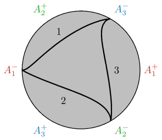
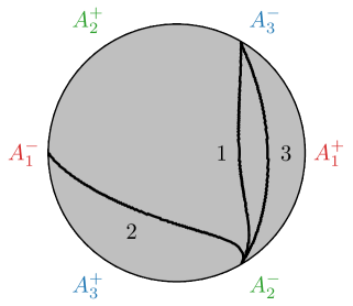
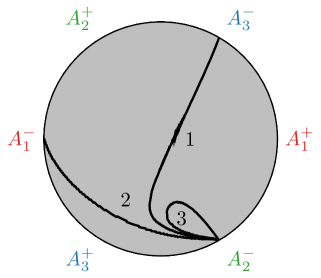
Figure 2: The equatorial plane is divided up by the stable manifolds of $B_{1}^{+}$,$B_{2}^{+}$,$B_{3}^{+}$ into basins of attraction of $A_{1}^{+},A_{2}^{+},A_{3}^{+},C^{+}$. Three possible divisions are shown, for the $+++$ case (left), the $++-$ case (middle) and the $+--$ case (right). The black curves are labelled to show which are the stable manifolds of $B_{1}^{+},B_{2}^{+},B_{3}^{+}$.

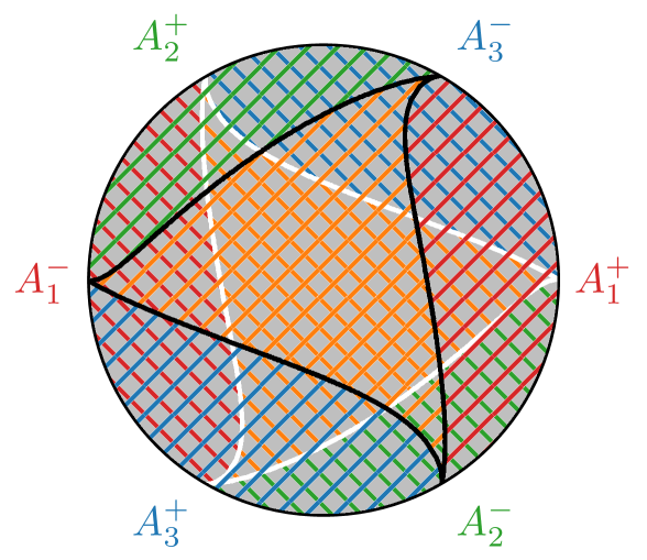
Figure 3: The equatorial plane with parameter values $\alpha_{1}=0.2,\alpha_{2}=0.3,\alpha_{3}=0.5$ ($+++$ case). The black curves are the stable manifolds of the $B^{+}$ points, the white curves are the unstable manifolds of the $B^{-}$ points. The color of the positively-sloped hatching in a region shows the limit of orbits in this region as $t\rightarrow+\infty$: red denotes $A_{1}^{+}$, green denotes $A_{2}^{+}$, blue denotes $A_{3}^{+}$, orange denotes $C^{+}$. Similarly the color of the negatively-sloped hatching shows the limit as $t\rightarrow-\infty$.

To establish the existence of orbits going from one of the $B^{-}$ or $C^{-}$ points to one of the $B^{+}$ or $C^{+}$ points we consider the division of the equatorial plane by both the stable manifolds of the $B^{+}$ points and the unstable manifolds of the $B^{-}$ points, the latter being obtained by a half turn from the former due to the $f(x)\rightarrow-f(-x)$ symmetry of $sP_{\mathrm{IV}}$. See Figures 3,4,5 for the $+++$, $++-$ and $+--$ cases respectively. In the $+++$ case it is clear that the rotated copy of each of the stable manifolds of the $B^{+}$ points (i.e. the unstable manifold of the corresponding $B^{-}$ point) must intersect the stable manifolds of the other two $B^{+}$ points. It follows, by simple topological arguments, that in the $+++$ case there must be at least one open region in the disk corresponding to solutions going from $C^{-}$ to $C^{+}$; there must be at least one curve segment corresponding to solutions going from $C^{-}$ to any of the $B^{+}$ points and from any of the $B^{-}$ points to $C^{+}$; and there must be at least one point corresponding to an orbit going from any of the points $B_{i}^{-}$ to the points $B_{j}^{+}$ with $j\not=i$. In the $++-$ case we obtain (at least) two curve segments corresponding to solutions going from $C^{-}$ to one of the $B^{+}$ points (as allowed by the rules in Table 2), and from one of the $B^{-}$ points to $C^{+}$. In addition, there are at least four $B$ to $B$ solutions. In the $+--$ case we obtain (at least) two $B$ to $B$ solutions. In short: solutions exhibiting every transition allowed by Table 2 appear, with the expected number of parameters ($2$ for $C$ to $C$, $1$ for $C$ to $B$ and $B$ to $C$, and isolated solutions for $B$ to $B$). This is the result on nonsingular solutions described in the Introduction. The only assumption that has been made on the parameters in reaching the result is that none of the $\alpha_{i}$ vanish. There is extensive discussion in the literature [3, 2, 17, 18] of real solutions of ($P_{\mathrm{IV}}$) in the case $\beta=0$, which is precisely the case that we have excluded. However, there are clear similarities between the existing results in the case $\beta=0$ and our results, presumably reflecting the fact that some properties persist in an appropriate limit as one of the $\alpha_{i}$ tends to zero.

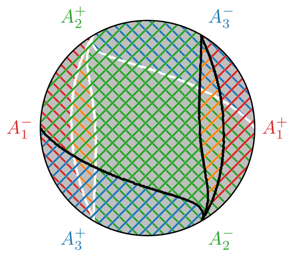
Figure 4: The equatorial plane with parameter values $\alpha_{1}=0.5,\alpha_{2}=0.7,\alpha_{3}=-0.2$ ($++-$ case). Coloring as in Figure 3.

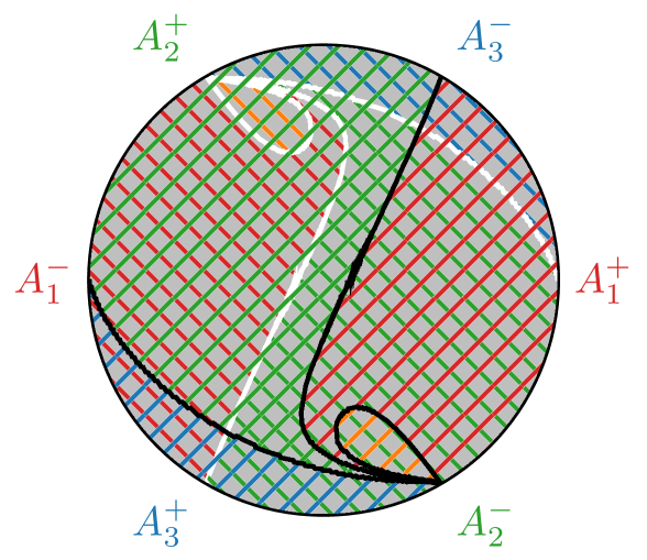
Figure 5: The equatorial plane with parameter values $\alpha_{1}=1.1,\alpha_{2}=-0.03,\alpha_{3}=-0.07$ ($+--$ case). Coloring as in Figure 3.

The $B$ to $B$ solutions are of some significance. At any of the $B$ points, one of the components $f_{1},f_{2},f_{3}$ diverges, but the others tend to zero. Thus one component of a $B_{i}^{-}$ to $B_{j}^{+}$ solution, with $i\not=j$, gives a solution of $P_{\mathrm{IV}}$ that is not only nonsingular on the entire real axis, but also tends to $0$ as $x\rightarrow\pm\infty$. Our results give methods for searching for these solutions, as they sit on the intersection of one $B^{+}$ stable manifold and one $B^{-}$ unstable manifold, thus corresponding to an initial value at which both the $x\rightarrow+\infty$ and the $x\rightarrow-\infty$ asymptotics changes. We show some relevant numerical results in Appendix B. Figures 8,9 illustrate in the $+++$ case. Figures 10,11,12,13 illustrate for the two different types of intersection point that occur in the $++-$ case. And Figures 14,15 illustrate in the $+--$ case. Note that in certain cases the $B$ to $B$ solutions have the further property of having no zeros on the entire real axis.

Finally in this section, we show some numerical results on the shape of the $C^{-}$ to $C^{+}$ region that exists in the $+++$ case. The numerical evidence we have points to there being only a single open region of such solutions in the space of initial data. In Figure 6 we plot the boundary of the relevant region in the space of initial data, for a variety of parameter values. As expected, we observe that as any of the parameters $\alpha_{i}$ gets smaller, the area of the region contracts.

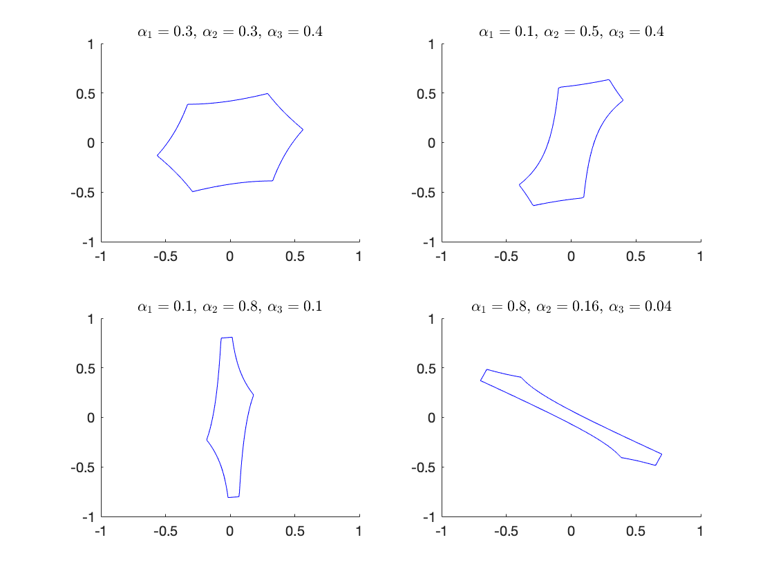
Figure 6: The region of $C$ to $C$ solutions in the space of initial values, for different sets of parameters in the $+++$ case. The horizontal axis is $f_{1}(0)$, the vertical axis is $\frac{f_{2}(0)-f_{3}(0)}{\sqrt{3}}$ and $f_{1}(0)+f_{2}(0)+f_{3}(0)=0$.

4 Solutions with Poles and Allowed Pole Sequences

In this section we consider solutions of $sP_{\mathrm{IV}}$ that have singularities. There clearly are four possibilities: a solution could have a finite sequence of singularities, or a singly infinite sequence with no singularities for $x$ less than a certain finite value, or a singly infinite sequence with no singularities for $x$ more than a certain finite value, or a doubly infinite sequence. In the first case, we need to specify the asymptotics of the solution as $x\rightarrow\pm\infty$, in the second case as $x\rightarrow-\infty$, and in the third case as $x\rightarrow+\infty$. We restrict ourselves to the generic case of type $C$ asymptotic behavior. The discussion can be extended to include type $B$ asymptotic behavior as well, but we do not pursue this here.

In the obvious manner we associate with each solution of this type a symbol sequence specifying the singularities and the asymptotic behavior. In the case of a finite sequence of singularities, the sequence begins and ends with $C$ and has a finite sequence of the symbols $A_{1},A_{2},A_{3}$ between the two $C$s. In the singly infinite case the sequence will begin or end with $C$, followed or preceded by an infinite sequence of $A$s. In the doubly infinite case the sequence just consists of $A$s. Table 1 shows that certain symbols cannot follow certain other symbols, depending on the signs of the parameters $\alpha_{i}$. We recall that these forbidden transitions are obtained by considering the signs of $f_{1},f_{2},f_{3}$ near the various singularities and in the appropriate asymptotic regimes (see equations (15) and (16) in [19]), and using the fact that the sign of $\alpha_{i}$ determines the sign of $f_{i}^{\prime}$ at a regular zero of $f_{i}$ (that is, at a zero where all components of the solution are nonsingular); thus between any two singularities, there can be at most one regular zero of each of the $f_{i}$, and the change in sign of $f_{i}$ at such a zero can only be in a specific direction. In the cases of permitted transitions, Table 1 also shows which of the functions $f_{1},f_{2},f_{3}$ have zeros (though note that the order of these zeros is not determined).

We now prove the following result:

Theorem.

In the case $\alpha_{1},\alpha_{2},\alpha_{3}>0$,

1. The only permitted finite singularity sequence is $CC$.

2. The only permitted singly infinite singularity sequences are

   $$\begin{array}[]{r}CA_{2}A_{1}A_{3}A_{2}A_{1}A_{3}A_{2}A_{1}\ldots\\ CA_{1}A_{3}A_{2}A_{1}A_{3}A_{2}A_{1}\ldots\\ CA_{3}A_{2}A_{1}A_{3}A_{2}A_{1}\ldots\end{array}$$ (8)

   and

   $$\begin{array}[]{l}\ldots A_{1}A_{2}A_{3}A_{1}A_{2}A_{3}A_{1}A_{2}C\\ \ldots A_{1}A_{2}A_{3}A_{1}A_{2}A_{3}A_{1}C\\ \ldots A_{1}A_{2}A_{3}A_{1}A_{2}A_{3}C\end{array}$$ (9)

3. The only permitted doubly infinite singularity sequences are

   $$\begin{array}[]{c}\ldots.A_{1}A_{2}A_{3}A_{1}A_{2}A_{3}~{}~{}~{}~{}~{}~{}~{}A_{1}~{}~{}~{}~{}~{}~{}~{}~{}A_{3}A_{2}A_{1}A_{3}A_{2}A_{1}\ldots\\ \ldots.A_{1}A_{2}A_{3}A_{1}A_{2}A_{3}~{}~{}~{}~{}A_{1}A_{2}A_{1}~{}~{}~{}~{}A_{3}A_{2}A_{1}A_{3}A_{2}A_{1}\ldots\\ \ldots.A_{1}A_{2}A_{3}A_{1}A_{2}A_{3}A_{1}A_{2}A_{3}A_{2}A_{1}A_{3}A_{2}A_{1}A_{3}A_{2}A_{1}\ldots\\ \end{array}$$ (10)

   or doubly infinite repetitions of the subsequences $A_{1}A_{2}A_{3}$ or $A_{3}A_{2}A_{1}$.

Proof.

From Table 1, in the case that all the $\alpha_{i}$ are positive, a singularity of type $A_{i}$ cannot be followed by another singularity of type $A_{i}$.

To obtain further restrictions on the permitted sequence of singularities, we consider the action of the symmetry group. Note that both the symmetries $\sigma$ and $\tau$ described in Section 2.2 preserve asymptotic type $C$ behavior. The action of $\sigma$ maps singularities of type $A_{i}$ to singularities of type $A_{i+1~{}{\rm mod}~{}3}$ and regular zeros of $f_{i}$ to regular zeros of $f_{i+1~{}{\rm mod}~{}3}$. A brief calculation shows that the action of $\tau$ does not affect type $A_{2}$ and type $A_{3}$ singularities, but eliminates type $A_{1}$ singularities, leaving regular zeroes of $f_{1}$ at the points of singularity; at the same time it creates new type $A_{1}$ singularities out of regular zeros of $f_{1}$ (and this is the only way the action of $\tau$ can create new singularities). Recall also that $\tau(\alpha_{1},\alpha_{2},\alpha_{3})=(-\alpha_{1},\alpha_{2}+\alpha_{1},\alpha_{3}+\alpha_{1})$ so after the action of $\tau$ the new value of $\alpha_{1}$ is negative, and the new values of $\alpha_{2},\alpha_{3}$ are still positive.

Suppose that a solution with $\alpha_{1},\alpha_{2},\alpha_{3}>0$ has symbol sequence $CA_{1}C$. From Table 1 we see that there are zeros of $f_{1}$ both between the first $C$ and the $A_{1}$, and between the $A_{1}$ and the second $C$. Thus applying $\tau$ gives the symbol sequence $CA_{1}A_{1}C$. But now $\alpha_{1}<0$ and $\alpha_{2},\alpha_{3}>0$, and we see from Table 1 that in this situation an $A_{1}$ singularity cannot follow another $A_{1}$ singularity. Thus we have a contradiction, and the symbol sequence $CA_{1}C$ is not permitted when $\alpha_{1},\alpha_{2},\alpha_{3}>0$. Similar arguments eliminate any symbol sequence containing any of the subsequences $CA_{1}A_{2}$, $A_{2}A_{1}C$ or $A_{2}A_{1}A_{2}$. Application of $\tau$ to any of these will lead to two consecutive $A_{1}$ singularities, which is not allowed.

Similarly, applying $\tau_{2}=\sigma^{2}\tau\sigma$ (which maps the parameters to $\alpha_{1}+\alpha_{2},-\alpha_{2},\alpha_{3}+\alpha_{2}$, i.e. to the $+-+$ case) eliminates the substrings $CA_{2}C$, $CA_{2}A_{3}$, $A_{3}A_{2}C$, $A_{3}A_{2}A_{3}$. and applying $\tau_{3}=\sigma\tau\sigma^{2}$ eliminates the substrings $CA_{3}C$, $CA_{3}A_{1}$, $A_{1}A_{3}C$, $A_{1}A_{3}A_{1}$.

Let us now consider a permitted sequence starting $CA_{1}$. The sequences $CA_{1}C$, $CA_{1}A_{2}$ and $A_{1}A_{1}$ are not allowed, so the sequence must in fact start with $CA_{1}A_{3}$. The sequences $A_{1}A_{3}A_{1}$, $A_{1}A_{3}C$ and $A_{3}A_{3}$ are not allowed, so the sequence must in fact start $CA_{1}A_{3}A_{2}$. Continuing, we reach the conclusion that the only permitted sequence starting $CA_{1}$ is the singly infinite sequence $CA_{1}A_{3}A_{2}A_{1}A_{3}A_{2}A_{1}\ldots$. Similarly we deduce that the only permitted sequence starting $CA_{2}$ is $CA_{2}A_{1}A_{3}A_{2}A_{1}A_{3}A_{2}A_{1}\ldots$ and the only permitted sequence starting $CA_{3}$ is $CA_{3}A_{2}A_{1}A_{3}A_{2}A_{1}A_{3}A_{2}A_{1}\ldots$.

This proves the section of the theorem relating to sequences (finite or singly infinite) starting with $C$. The section relating to singly infinite sequences ending in $C$ is proved similarly. For doubly infinite sequences, it is straightforward to show that the subsequences $A_{3}A_{1}A_{3}$, $A_{1}A_{2}A_{1}$, $A_{2}A_{3}A_{2}$ have unique doubly infinite extensions, and the only other possible doubly infinite sequences of $A$s that are not excluded are doubly infinite repetitions of one of the subsequences $A_{1}A_{2}A_{3}$ or $A_{3}A_{2}A_{1}$. ∎

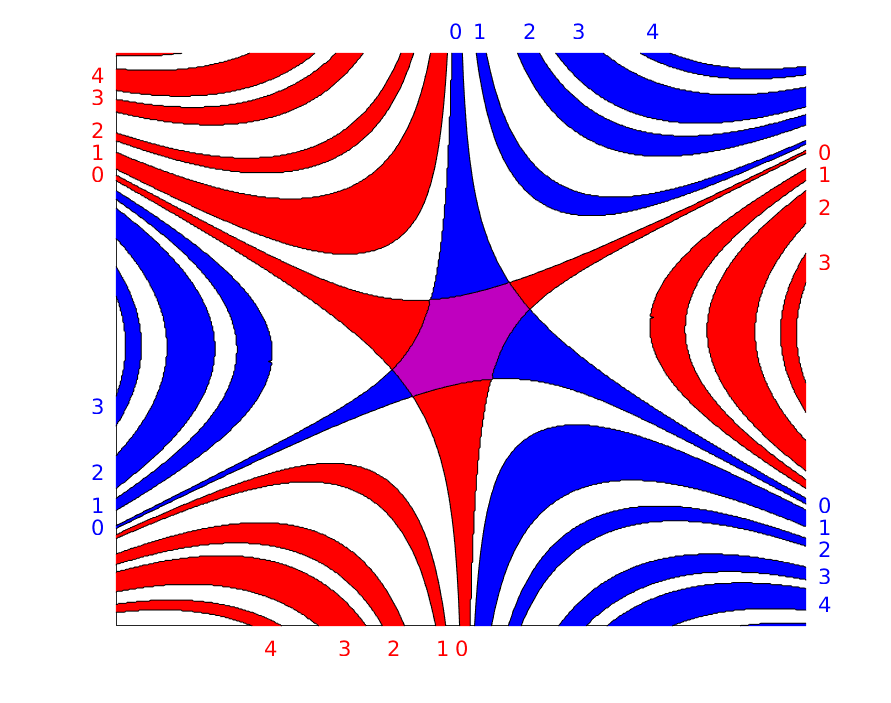
Figure 7: Types of solution for different initial conditions. Parameter values are $\alpha_{1}=0.2,\alpha_{2}=0.3,\alpha_{3}=0.5$. The horizontal axis is $f_{1}(0)$, the vertical axis is $\frac{f_{2}(0)-f_{3}(0)}{\sqrt{3}}$, both ranging approximately from $-3$ to $3$. Purple region: nonsingular solutions. Blue regions: An infinite number of singularities in $x<0$ and a finite number in $x>0$, with the number of singularities in $x>0$ marked for each region. Red regions: the same, reversed. White regions: an infinite sequence of singularities in both $x>0$ and $x<0$.

Numerical experiments show that in practice there exist solutions with no singularities, as we have already documented; there also exist solutions with all the possible singly infinite singularity sequences, and solutions with the first 3 types of doubly infinite singularity sequence. We have not yet found evidence of the last two possibilities, viz. doubly infinite repetitions of one the subsequences $A_{1}A_{2}A_{3}$ or $A_{3}A_{2}A_{1}$. In Figure 7 we show numerical results for one specific choice of the parameters (using the numerical method explained in Appendix A for integrating through poles). For different choices of initial condition at $x=0$ we integrate up to $x=10$ and down to $x=-10$ and count the number of poles in $x>0$ and in $x<0$. For the purpose of the experiment any number of poles exceeding $10$ is considered to be infinite. We find “bands” in the plane of initial values with $0,1,2,3,\ldots$ poles in $x>0$, and corresponding bands (related by the symmetry $f(x)\rightarrow-f(-x)$) with $0,1,2,3,\ldots$ poles in $x<0$. The only intersection of the bands is apparently a single region giving pole-free solutions. Between the bands we observe regions where there are presumably solutions with doubly infinite singularity sequences. In the regions corresponding to singly infinite singularity sequences we observe cases with the “last” singularity being of all $3$ possible types, as shown in (8) and (9); in the doubly infinite bands we observe cases with the “central” singularity being of all $3$ possible types given in (10). However, we do not observe cases where the singularity sequence is a doubly infinite repetition of the subsequences $A_{1}A_{2}A_{3}$ or $A_{3}A_{2}A_{1}$.

Many related plots can be found in the numerical work of Reeger and Fornberg [17, 18]. Much of Reeger and Fornberg’s work relates to nongeneric parameter values, but Figure 8 in [18] relates to the case $\alpha_{1}=\alpha_{2}=\frac{1}{4}$, $\alpha_{3}=\frac{1}{2}$, and shows what appears to be two regions in the space of initial values for which there is a pole-free solution. This arises as $u(0)$ and $u^{\prime}(0)$ in Reeger and Fornberg’s work correspond to $f_{1}(0)$ and $-\frac{1}{2}+f_{1}(0)(f_{2}(0)-f_{3}(0))$ in our work.

The results for the case that $\alpha_{1},\alpha_{2},\alpha_{3}$ are all positive can be generalized using the transformation group to appropriate results for any generic choice of parameters. To see the effect of the transformation $\tau$ on a particular singularity sequence (for a particular set of parameters), we use Table 1 to locate the zeros of $f_{1}$ (inserting an appropriate symbol, say $Z_{1}$), then we delete the existing $A_{1}$s and replace the $Z_{1}$s by new $A_{1}$s. The effect of the transformation $\sigma$ is simply to cycle $A_{1},A_{2},A_{3}$. Clearly doubly infinite sequences remain doubly infinite, singly infinite sequences remain singly infinite, and finite sequences remain finite. Thus we arrive at the results stated in the Introduction: for any generic choice of the parameters, there exists a unique finite sequence of singularities for which $sP_{\mathrm{IV}}$ has a two-parameter family of solutions with this singularity sequence. The (singly and doubly) infinite sequences that are permitted in general also depend on the values of the parameters. For example, by application of $\tau$ to the sequence

$$\ldots A_{1}A_{2}A_{3}A_{1}A_{2}A_{3}~{}~{}~{}~{}A_{1}~{}~{}~{}~{}A_{3}A_{2}A_{1}A_{3}A_{2}A_{1}\ldots$$

that is permitted in the $+++$ case, we obtain the same sequence with the “central” $A_{1}$ removed, i.e.

$$\ldots A_{1}A_{2}A_{3}A_{1}A_{2}A_{3}~{}~{}~{}~{}~{}~{}~{}~{}A_{3}A_{2}A_{1}A_{3}A_{2}A_{1}\ldots$$

(note that a repeated $A_{3}$ is allowed in the case $-++$). The two sequences consisting of doubly infinite repetitions of $A_{1},A_{2},A_{3}$ or $A_{3},A_{2},A_{1}$ seem to be allowed for arbitrary values of the parameters. They are evidently invariant under the action of $\sigma$, and in fact are also invariant under the action of $\tau$ except in the case $--+$. In this case both are transformed to the sequence which is a doubly infinite repetition of the subsequence $A_{2}A_{3}$ (which seems to be allowed in the cases $+-+$ and $+--$, but we have not observed its existence).

5 Special Solutions

5.1 Rational Solutions 1

In this section we consider the rational solutions of $sP_{\mathrm{IV}}$ that are equivalent to the so-called “$-\frac{2}{3}z$ hierarchy” of $P_{\mathrm{IV}}$ [7]. These occur when the parameters take values at the centers of faces of the lattice in Figure 1. The fundamental example is the solution $f_{1}=f_{2}=f_{3}=\frac{1}{3}x$ that is obtained when $\alpha_{1}=\alpha_{2}=\alpha_{3}=\frac{1}{3}$. Indeed the general solution of this kind is obtained by application of an arbitrary element of the symmetry group on this fundamental solution [14, 16]. Thus for example, by applying $\tau\sigma^{2}\tau$ to the fundamental solution we obtain the solution

$$f_{1}=\frac{x^{2}-3}{3x}\ ,f_{2}=\frac{x(x^{2}+3)}{3(x^{2}-3)}\ ,f_{3}=\frac{x^{4}-6x^{2}-9}{3x(x^{2}-3)}\ ,$$

for parameter values $\alpha_{1}=-\frac{2}{3},\alpha_{2}=\frac{1}{3},\alpha_{3}=\frac{4}{3}$. In the context of this paper, this result is useful as by looking at the singularities of the rational solution we can determine the unique finite singularity sequence of solutions for all values of the parameters in the cell whose center gives the rational solution. In the case of the example just given, there are singularities at $x=0,\pm\sqrt{3}$ and the sequence is $CA_{1}A_{2}A_{1}C$. This sequence can be read off from the group element that generated the solution. The fundamental solution has singularity sequence $CC$, applying $\tau$ gives the sequence $CA_{1}C$ (and parameter values $-++$), applying $\sigma^{2}$ gives the sequence $CA_{2}C$ (and parameter values $+-+$), and applying $\tau$ again gives the sequence $CA_{1}A_{2}A_{1}C$. Note that in the context of studies of the distribution of singularities of rational solutions in the complex plane [12, 10], no rules are currently known for evaluating the effect of the transformation $\tau$.

We also note the following fact: If the action of the group element $g$ on the fundamental solution gives $f$ for parameter values $\alpha$, then using the obvious notation we have

$$(g^{-1}f)_{1}=(g^{-1}f)_{2}=(g^{-1}f)_{3}\ .$$

This gives two polynomial equations that must be satisfied by the components of the rational solution $f$, in addition to the constraint $f_{1}+f_{2}+f_{3}=x$. Thus, in the above example, it is possible to check that

$$9f_{1}^{2}f_{2}^{2}-9f_{1}^{2}f_{2}f_{3}+3f_{1}^{2}-18f_{1}f_{2}+6f_{1}f_{3}+8 = 0$$

$$-9f_{1}^{3}f_{2}+9f_{1}^{2}f_{2}f_{3}+6f_{1}f_{2}-6f_{1}f_{3}-4 = 0$$

As far as we are aware, these polynomial relations between the components of a rational solution are new.

5.2 Rational Solutions 2

In this section we consider the rational solutions of $sP_{\mathrm{IV}}$ that are equivalent to the so-called “$-2z$ hierarchy” and “$-\frac{1}{z}$ hierarchy” of $P_{\mathrm{IV}}$ [7]. These occur when the parameters take values at the vertices of the lattice in Figure 1. The simplest example is the solution $f_{1}=x$, $f_{2}=f_{3}=0$ that is obtained when $\alpha_{1}=1$, $\alpha_{2}=\alpha_{3}=0$. A complication arises that does not occur for the first set of rational solutions: Applying the transformation $\tau$ requires that $f_{1}$ should be nonzero, and $f_{1}$ can be zero in the case that $\alpha_{1}=0$. The general rational solution of the second type arises by application of a restricted set of group elements to the fundamental solution, those that avoid generating the parameter value $\alpha_{1}=0$ as an intermediate step. However, there is no shortage of group elements with this property. The resulting solutions also satisfy polynomial identities, in this case obtained from the conditions

$$(g^{-1}f)_{2}=(g^{-1}f)_{3}=0\ .$$

As an example, application of the group element $\sigma\tau\sigma^{2}\tau\sigma^{2}\tau\sigma\tau\sigma\tau$ to the fundamental solution gives

$$f_{1}=\frac{2x(x^{2}-3)(x^{2}+1)}{(x^{2}-1)(x^{4}+3)}\ ,f_{2}=\frac{-2x(x^{2}-1)(x^{2}+3)}{(x^{2}+1)(x^{4}+3)}\ ,f_{3}=\frac{x(x^{4}+3)}{(x^{2}-1)(x^{2}+1)}\ ,$$

for parameter values $\alpha_{1}=\alpha_{2}=2,\alpha_{3}=-3$. These functions obey the polynomial identities

$$f_{1}^{2}f_{2}f_{3}^{2}+f_{1}^{2}f_{3}-5f_{1}f_{2}f_{3}-f_{1}f_{3}^{2}-3f_{1}+6f_{2}+2f_{3} = 0\ ,$$

$$f_{1}f_{2}^{2}f_{3}^{2}+5f_{1}f_{2}f_{3}-f_{2}^{2}f_{3}+f_{2}f_{3}^{2}+6f_{1}-3f_{2}+2f_{3} = 0\ .$$

Although we have not discussed solutions with singularities with $B$ type asymptotics in this paper, we mention that this solution has singularity sequence $B_{3}A_{2}A_{2}B_{3}$.

It is straightforward to establish that there is a rational solution of $sP_{\mathrm{IV}}$ with $f_{1}=0$ (and thus $\alpha_{1}=0$) for arbitrary integer values of $\alpha_{2},\alpha_{3}$ with $\alpha_{2}+\alpha_{3}=1$. For positive integer values of $\alpha_{2}$ the solution has

$$f_{2}(x)=\frac{\sqrt{2}\alpha_{2}{\rm He}_{\alpha_{2}}\left(\frac{ix}{\sqrt{2}}\right)}{i{\rm He}_{\alpha_{2}}^{\prime}\left(\frac{ix}{\sqrt{2}}\right)}\ ,f_{3}=x-f_{2}\ ,$$

where ${\rm He}_{n}$ denotes the $n$th Hermite polynomial. This has singularity sequence $B_{2}B_{2}$ for odd values of $\alpha_{2}$ and $B_{2}A_{1}B_{2}$ for even values of $\alpha_{2}$. For nonpositive integer values of $\alpha_{2}$ the solution is

$$f_{2}(x)=-\frac{{\rm He}_{-\alpha_{2}}^{\prime}\left(\frac{x}{\sqrt{2}}\right)}{\sqrt{2}{\rm He}_{-\alpha_{2}}\left(\frac{x}{\sqrt{2}}\right)}\ ,f_{3}=x-f_{2}\ .$$

This has singularity sequence $B_{3}A_{1}\ldots A_{1}B_{3}$ with $-\alpha_{2}$ successive singularities of type $A_{1}$. Note that since these solutions have $\alpha_{1}=0$ the rules of Table 1 do not apply. However, since successive $A_{1}$ singularities are allowed in both the cases $+-+$ and $--+$, it is not surprising that we also see this on the transition between them. Note also that these solutions have all their singularities on the real axis, with no further poles in the complex plane.

5.3 Other Special Solutions

In greater generality, whenever $\alpha_{1}=0$, $sP_{\mathrm{IV}}$ has a 1-parameter family of solutions with $f_{1}=0$. In this case the $sP_{\mathrm{IV}}$ system reduces to the first order Riccati equation

$$f_{2}^{\prime}=f_{2}(x-f_{2})+\alpha_{2}\ ,$$

which can be linearized. By application of suitable group elements, these solutions give rise to a 1-parameter family of solutions whenever any of the $\alpha_{i}$ takes an integer value. In fact, these solutions (and the corresponding solutions of $P_{\mathrm{IV}}$) can all be obtained as the solution of a first order differential equation. To see this, note that by application of the inverse group element to the solution, it must satisfy the single polynomial identity

$$(g^{-1}f)_{1}=0\ .$$

Substituting

$$f_{2}=\frac{1}{2}\left(x-f_{1}+\frac{f_{1}^{\prime}-\alpha_{1}}{f_{1}}\right)\ ,\qquad f_{3}=\frac{1}{2}\left(x-f_{1}-\frac{f_{1}^{\prime}-\alpha_{1}}{f_{1}}\right)$$

gives a first order differential equation for $f_{1}$. Thus, for example, by applying the transformation $\sigma^{2}\tau\sigma^{2}\tau\sigma\tau\sigma^{2}\tau\sigma^{2}\tau\sigma$ to the solutions with $f_{1}=0$ we obtain the set of special solutions with $\alpha_{1}=2$, and these give rise to the special solutions of $P_{\mathrm{IV}}$, equation (1), with $\beta=-8$, that satisfy the first order differential equation

$$0 = \left(\frac{\mathrm{d}w}{\mathrm{d}z}\right)^{4}+8\,\left(\frac{\mathrm{d}w}{\mathrm{d}z}\right)^{3}+\left(-2w^{4}-8zw^{3}-8(z^{2}-\alpha)w^{2}\right)\left(\frac{\mathrm{d}w}{\mathrm{d}z}\right)^{2}+\left(-8w^{4}-32zw^{3}-32(z^{2}-\alpha)w^{2}-128\right)\left(\frac{\mathrm{d}w}{\mathrm{d}z}\right)$$

$$+w^{8}+8zw^{7}+8(3z^{2}-\alpha)w^{6}+32z(z^{2}-\alpha)w^{5}+16\left((z^{2}-\alpha)^{2}+1\right)w^{4}+64zw^{3}-256$$

Thus there are first order equations of higher and higher degree that are consistent with $P_{\mathrm{IV}}$ for suitable values of the parameters. This generalizes the old observation that for suitable values of the parameters $P_{\mathrm{IV}}$ is consistent with a Riccati equation [13].

6 Concluding Remarks

In the course of this paper a framework has emerged for classification of real solutions of $sP_{\mathrm{IV}}$ (and thus also for $P_{\mathrm{IV}}$): a solution is classified by its asymptotic behavior as $x\rightarrow\pm\infty$ and its singularity sequence, with the asymptotic behavior being superfluous in one or both limits in the cases of singly infinite or doubly infinite singularity sequences respectively. We have established a strong result for the existence of solutions with no singularities. For the case of nonzero parameter values, solutions exist exhibiting all the transitions allowed by Table 2. For the case of solutions with singularities and with generic ($C$-type) asymptotic behavior (if needed), we have given a list of the possible singularity sequences in the $+++$ parameter case, from which a similar list can be derived for an arbitrary generic (noninteger) set of parameters. In particular we have seen that for any generic set of parameters there is a unique allowed finite singularity sequence for solutions with $C$ to $C$ asymptotics. Numerics in the $+++$ case indicate that all the permitted singularity sequences actually occur, with the possible exception of doubly infinite repetitions of the subsequences $A_{1}A_{2}A_{3}$ and $A_{3}A_{2}A_{1}$. We are hopeful that it might be possible to exclude these possibilities using techniques not considered in the current paper; it is well-known that there are solutions of $P_{\mathrm{IV}}$ with elliptic function asymptotics for large argument [20], and this is a question about the connection formulae for these solutions.

Our work has all been on the basis of an assumption concerning the dynamical system described in our previous work [19]. We are happy with this assumption as there is no evidence to the contrary, and it is an assumption of the simplest possible scenario (that the only possible asymptotics are the $B$ and $C$ behaviors we have described). However proving it looks difficult, as it involves the local stability properties of a periodic orbit in the case that the linearized approximation gives insufficient information.

We believe the approach given here for $P_{\mathrm{IV}}$ should be extendable to other Painlevé equations. Relevant dynamical systems have been given in [1, 21]. However, the works of Chiba [5, 6] suggest that more subtle compactifications will be involved.

Appendix A Numerical Methods for Integrating Through Poles

We use the following simple idea to construct changes of the dependent variables that allow us to integrate through the three types of pole singularity of $sP_{\mathrm{IV}}$. Near the $A_{3}$ type singularity the system has a Painlevé series as given by Equation (15) in [19]. This expresses $f_{1},f_{2},f_{3}$ in terms of three quantities $x-x_{0},x_{0},C$ all of which remain finite near the pole. Truncating this expansion in such a way that $f_{1}$ depends only on the first quantity (which we call $z_{1}$), $f_{2}$ depends only on the first and second (which we call $2z_{2}$), and $f_{3}$ depends on the first, the second and the third (which we call $-2z_{3}$) but on the latter only linearly, gives the substitution

$$f_{1} = \frac{1}{z_{1}}\ ,$$

$$f_{2} = -\frac{1}{z_{1}}+z_{2}\ ,$$

$$f_{3} = -\alpha_{3}z_{1}+z_{3}z_{1}^{2}\ .$$

This is, by construction, an invertible change of variables, with inverse

$$z_{1} = \frac{1}{f_{1}}\ ,$$

$$z_{2} = f_{1}+f_{2}\ ,$$

$$z_{3} = \alpha_{3}f_{1}+f_{1}^{2}f_{3}\ .$$

The variables $z_{1},z_{2},z_{3}$ satisfy the system

$$z_{1}^{\prime} = 1+z_{1}\left(z_{1}^{2}z_{3}-z_{1}(\alpha_{1}+\alpha_{3})-z_{2}\right)\ ,$$

$$z_{2}^{\prime} = 1+\alpha_{3}+z_{1}\left(z_{1}z_{2}z_{3}-(2+\alpha_{3})z_{3}\right)\ ,$$

$$z_{3}^{\prime} = z_{2}z_{3}-\alpha_{3}(\alpha_{1}+\alpha_{3})+z_{1}z_{3}\left(2\alpha_{1}+3\alpha_{3}-2z_{1}z_{3}\right)\ .$$

As soon as a pole of the appropriate type in the $f$ system is approached (say if $|f_{1}|,|f_{2}|>10$) we change to the $z$ variables and integrate there until the pole is passed. Similar changes of variables are used near the other two types of pole.

Appendix B Numerics for $B$ to $B$ solutions

As visible from Figures 3,4,5, solutions with $B$ to $B$ type asymptotics occur at the crossing points of the stable manifolds of the $B^{+}$ points with the unstable manifolds of the $B^{-}$ points. It is possible to numerically search for these solutions by locating four points in the four regions adjacent to the crossing, distinguished by the associated asymptotic behaviors as $t\rightarrow\pm\infty$, and then recursively reducing the size of the associated quadrilateral (as measured by its perimeter) until the crossing point is found to sufficient accuracy. The following plots show some examples. Figures 8,9 are relevant to one of the $6$ crossing points in the $+++$ case. Figure 8 shows the different asymptotics in the four adjacent regions, and 9 shows the $B$ to $B$ solution once the initial condition has been found to sufficient accuracy to give an accurate plot on the interval $[-10,10]$. Figures 10,11,12,13 illustrate for the two different types of intersection point that occur in the $++-$ case. In one case the resulting $B$ to $B$ solution has no zeros in any components, in the other there is a zero in one component (see Table 2). Finally, Figures 14,15 illustrate in the $+--$ case.

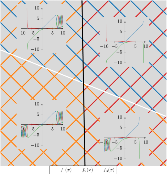
Figure 8: A zoomed-in version of the first-quadrant intersection in Figure 3.

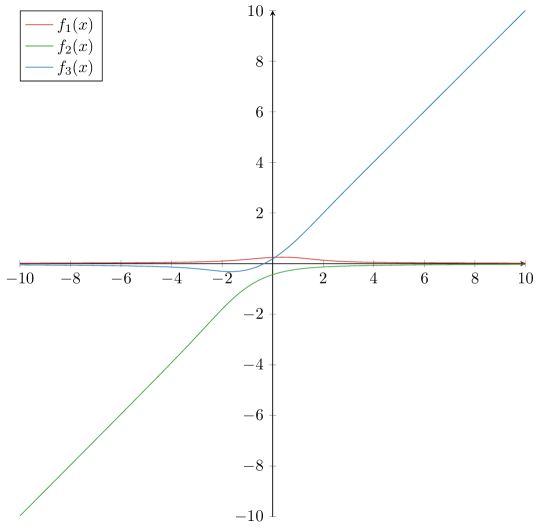
Figure 9: The $B_{2}^{-}\to B_{3}^{+}$ solution corresponding to the intersection in Figure 8.

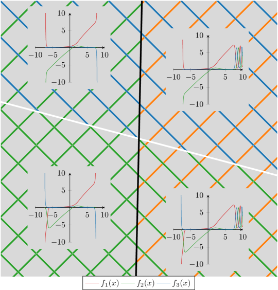
Figure 10: A zoomed-in version of a first-quadrant intersection in Figure 4.

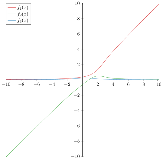
Figure 11: The $B_{2}^{-}\to B_{1}^{+}$ solution corresponding to the intersection in Figure 10.

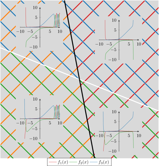
Figure 12: A zoomed-in version of the second first-quadrant intersection in Figure 4.

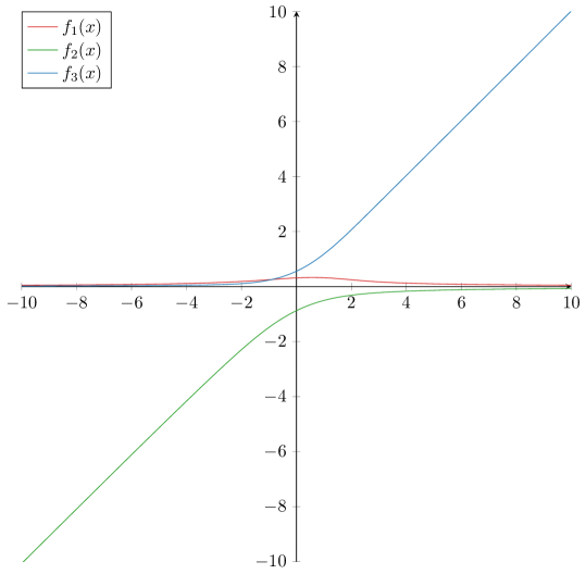
Figure 13: The $B_{2}^{-}\to B_{3}^{+}$ solution corresponding to the intersection in Figure 12.

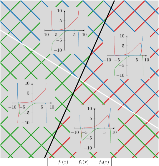
Figure 14: A zoomed-in version of the first-quadrant intersection in Figure 5.

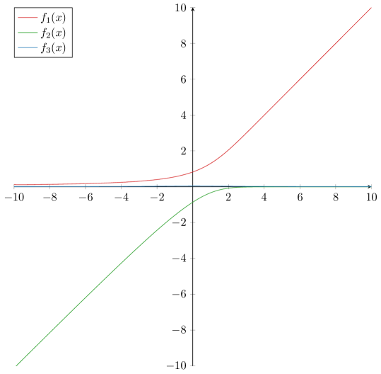
Figure 15: The $B_{2}^{-}\to B_{1}^{+}$ solution corresponding to the intersection in Figure 14.

References

- [1] Adler, V. E. Nonlinear chains and Painlevé equations. Phys. D 73, 4 (1994), 335–351.
- [2] Bassom, A. P., Clarkson, P. A., and Hicks, A. C. Numerical studies of the fourth Painlevé equation. IMA Journal of Applied Mathematics 50, 2 (1993), 167–193.
- [3] Bassom, A. P., Clarkson, P. A., Hicks, A. C., and McLeod, J. B. Integral equations and exact solutions for the fourth Painlevé equation. Proc. Roy. Soc. London Ser. A 437, 1899 (1992), 1–24.
- [4] Bureau, F. J. Differential equations with fixed critical points. In Painlevé transcendents (Sainte-Adèle, PQ, 1990), vol. 278 of NATO Adv. Sci. Inst. Ser. B Phys. Plenum, New York, 1992, pp. 103–123.
- [5] Chiba, H. The first, second and fourth Painlevé equations on weighted projective spaces. J. Differential Equations 260, 2 (2016), 1263–1313.
- [6] Chiba, H., et al. The third, fifth and sixth painlevé equations on weighted projective spaces. SIGMA. Symmetry, Integrability and Geometry: Methods and Applications 12 (2016), 019.
- [7] Clarkson, P. A. The fourth Painlevé equation and associated special polynomials. Journal of Mathematical Physics 44, 11 (2003), 5350–5374.
- [8] Clarkson, P. A. Painlevé equations—nonlinear special functions. In Orthogonal polynomials and special functions. Springer, 2006, pp. 331–411.
- [9] Clarkson, P. A. The fourth Painlevé transcendent. Differential Algebra and Related Topics II, Li Guo and WY Sit (eds.) (2008).
- [10] Clarkson, P. A., Gómez-Ullate, D., Grandati, Y., and Milson, R. Rational solutions of higher order painlev’e systems i. arXiv preprint arXiv:1811.09274 (2018).
- [11] NIST Digital Library of Mathematical Functions. http://dlmf.nist.gov/, Release 1.0.22 of 2019-03-15. F. W. J. Olver, A. B. Olde Daalhuis, D. W. Lozier, B. I. Schneider, R. F. Boisvert, C. W. Clark, B. R. Miller and B. V. Saunders, eds.
- [12] Filipuk, G. V., and Clarkson, P. A. The symmetric fourth painlevé hierarchy and associated special polynomials. Studies in Applied Mathematics 121, 2 (2008), 157–188.
- [13] Fokas, A. S., and Ablowitz, M. J. On a unified approach to transformations and elementary solutions of Painlevé equations. Journal of Mathematical Physics 23, 11 (1982), 2033–2042.
- [14] Murata, Y. Rational solutions of the second and the fourth painlevé equation. Funkcialaj Ekvacioj 28 (1985), 1–32.
- [15] Noumi, M., and Yamada, Y. Affine weyl groups, discrete dynamical systems and Painlevé equations. Comm. Math. Phys. 199, 2 (1998), 281–295.
- [16] Noumi, M., and Yamada, Y. Symmetries in the fourth Painlevé equation and Okamoto polynomials. Nagoya Mathematical Journal 153 (1999), 53–86.
- [17] Reeger, J. A., and Fornberg, B. Painlevé IV with both parameters zero: a numerical study. Studies in Applied Mathematics 130, 2 (2013), 108–133.
- [18] Reeger, J. A., and Fornberg, B. Painlevé IV: A numerical study of the fundamental domain and beyond. Physica D: Nonlinear Phenomena 280 (2014), 1–13.
- [19] Schiff, J., and Twiton, M. A dynamical systems approach to the fourth Painlevé equation. Journal of Physics A: Mathematical and Theoretical 52, 14 (2019), 145201.
- [20] Vereshchagin, V. L. Global asymptotics for the fourth Painlevé transcendent. Mat. Sb. 188, 12 (1997), 11–32.
- [21] Willox, R., and Hietarinta, J. Painlevé equations from Darboux chains. I. –. J. Phys. A 36, 42 (2003), 10615–10635.