Theory of coherent active convolved illumination for superresolution enhancement

Abstract

Recently an optical amplification process called the plasmon injection scheme was introduced as an effective solution to overcoming losses in metamaterials. Implementations with near-field imaging applications have indicated substantial performance enhancements even in the presence of noise. This powerful and versatile compensation technique, which has since been renamed to a more generalized active convolved illumination, offers new possibilities of improving the performance of many previously conceived metamaterial-based devices and conventional imaging systems. In this work, we present the first comprehensive mathematical breakdown of active convolved illumination for coherent imaging. Our analysis highlights the distinctive features of active convolved illumination, such as selective spectral amplification and correlations, and provides a rigorous understanding of the loss compensation process. These features are achieved by an auxiliary source coherently superimposed with the object field. The auxiliary source is designed to have three important properties. First, it is correlated with the object field. Second, it is defined over a finite spectral bandwidth. Third, it is amplified over that selected bandwidth. We derive the variance for the image spectrum and show that utilizing the auxiliary source with the above properties can significantly improve the spectral signal-to-noise ratio and resolution limit. Besides enhanced superresolution imaging, the theory can be potentially generalized to the compensation of information or photon loss in a wide variety of coherent and incoherent linear systems including those, for example, in atmospheric imaging, time-domain spectroscopy, ${\cal PT}$ symmetric non-Hermitian photonics, and even quantum computing.

I Introduction

Metamaterials (MMs), which are artificial inhomogeneous structures usually designed with subwavelength metal/dielectric or all-dielectric building blocks, rose to prominence nearly two decades ago as an appealing direction for designing materials with unprecedented electromagnetic properties previously considered difficult, if not impossible, to realize. Invisibility cloaks Schurig et al. (2006), ultra-high-resolution imaging Pendry (2000); Taubner et al. (2006); Jacob et al. (2006) and photolithography Gao et al. (2015), enhanced photovoltaics Gwamuri et al. (2013); Vora et al. (2014), miniaturized antennas Odabasi et al. (2013), ultrafast optical modulation Neira et al. (2014), and metasurfaces Arbabi et al. (2015); Genevet et al. (2017) are few of the multitude of applications which have been envisioned. Supported by parallel efforts in micro and nanofabrication, MMs are anticipated to have broad impact on many technologies employing electromagnetic radiation. However, despite enormous theoretical and experimental progress, numerous lingering problems Soukoulis and Wegener (2011) require diligent consideration. Optical losses continue to be one of the greatest threats to the viability of many of the MM-based devices proposed to date. Mitigation of losses remains a challenging problem for the MM community. Gain medium was initially proposed Ramakrishna and Pendry (2003); Vincenti et al. (2009); Wuestner et al. (2010); Xiao et al. (2010) as a potential solution. However, later studies showed that stability and gain saturation issues as a result of stimulated emission near the field enhancement regions leads to intense noise generation Soukoulis and Wegener (2010); Stockman (2007); Kinsler and McCall (2008). Due to these concerns and other associated complexities such as pump requirement, progress towards the development of a robust loss compensation scheme has been somewhat sluggish even after nearly two decades of efforts. Dielectric metasurfaces have also been proposed to alleviate some of these concerns Arbabi et al. (2015); Genevet et al. (2017).

A recent theoretical study Sadatgol et al. (2015) investigated an unconventional approach in the form of an alternative exploration of “virtual gain” Li et al. (2020); Ghoshroy et al. (to be published) to manage the losses in MMs. This compensation process, designated “plasmon injection (PI or $\Pi$) scheme,” employs an additional source to modify the field incident on a lossy MM. This auxiliary source is designed to adequately amplify an arbitrary field thereby enhancing its transmission through the MM. A multiport MM structure was used in Sadatgol et al. (2015) to illustrate the conceptual operating principle for the amplification of normally incident waves. Auxiliary fields are used to coherently add energy to the lossy system to compensate the losses of different natures. This amplification mechanism was related in Krasnok and Alu (2020); Ghoshroy et al. (to be published) to coherent amplification of pulses using a passive cavity described in Jones and Ye (2002); Potma et al. (2003). The main difference in Sadatgol et al. (2015) is continuous wave operation at the nanoscale plasmonic MM structure. In Ghoshroy et al. (2017, 2018a, 2018b), we discussed in detail the generalization of the $\Pi$ scheme to imaging, which involves a spectrum of spatial frequencies. A systematic amplification in the Fourier spectrum plays a key role in extending the resolution limit of the imaging system. This is akin to the Wiener optimal filtering principle that also attempts to cleverly privilege spatial frequencies with respect to their noises Roggemann et al. (1992); Biemond et al. (1990); Zaknich (2005). The earlier theoretical studies with MM or near-field imaging systems employing negative index materials (NIMs) Adams et al. (2016), superlenses Adams et al. (2017), and hyperlenses Zhang et al. (2016, 2017) produced promising results. Implementing the $\Pi$ scheme with the above systems resulted in performance improvements. The distinguishing feature of the $\Pi$ scheme is the auxiliary source. The earlier variants of the $\Pi$ scheme were shown to emulate linear deconvolution Adams et al. (2016).

The physical generation of the auxiliary source requires some considerations. It was shown Ghoshroy et al. (2017) that the auxiliary source can be generated through a convolution process with the original object field incident at the detector while selectively providing amplification to a controllable band of spatial frequencies. As a result of this process, the auxiliary source becomes correlated with the original object field Ghoshroy et al. (2017); Qian et al. (2017). A near-field spatial filter designed with hyperbolic metamaterials (HMMs) was proposed to physically generate the auxiliary source Ghoshroy et al. (2018a) with the above properties. The filter was integrated with a $50\,$nm silver film to illustrate the overall loss compensation process. This was the first potential application of the spatial filtering properties Schurig and Smith (2003); Rizza et al. (2012); Liu et al. (2017); Liang et al. (2018); Kieliszczyk et al. (2018) of HMMs in the context of loss compensation. Later studies with coherent Ghoshroy et al. (2018b) and incoherent Adams et al. (2018) illumination produced favourable results. An improvement in the resolution limit of a near-field silver superlens elevated the viability of the $\Pi$ scheme as an effective alternative to previously conceived loss mitigation approaches Ramakrishna and Pendry (2003); Popov and Shalaev (2006); Güney et al. (2009); Vora et al. (2014); Vincenti et al. (2009); Wuestner et al. (2010); Xiao et al. (2010) including dielectric metasurfaces Arbabi et al. (2015); Genevet et al. (2017). Even though the techniques presented in Ghoshroy et al. (2018b); Adams et al. (2018) possess similar properties to the original concept of the $\Pi$ scheme in Sadatgol et al. (2015), the scheme was generalized to a more encompassing term active convolved illumination (ACI) in Adams et al. (2018), since it is essentially the physical convolution operation which is key to the process. Also, the $\Pi$ scheme narrows down the process to only plasmons. More recently, the ACI technique has been applied to an experimental system, where the signal-to-noise ratio (SNR) and resolution limit of a reference far-field imaging system have been significantly improved with a modest amount of amplification Adams (2019). It has also been shown that the ACI offers more tolerance to pixel saturation compared to the reference system.
In this paper, we construct a theoretical framework to provide the first comprehensive mathematical exposition of the fundamental concept of ACI for coherent illumination. Pendry’s classic setup Pendry (2000) of a silver superlens operating at a wavelength of $365\,$nm is adopted since it is the simplest configuration which broadly exemplifies the rudimentary impact of optical losses such as in not only MM systems, but also different conventional and advanced linear systems. We consider the silver superlens only as a canonical example to accentuate how the ACI permits recovery of information carried by attenuated signal with minimal noise amplification. The greater scope of this paper is to develop a noise-resistant imaging theory that can be potentially generalized to a wide range of problems in various contexts related to noisy linear systems. Specific attention is drawn towards the required mechanisms, such as selective spectral amplification, physical convolution, and correlations. This study strengthens analytically, the previous results and associated assertions Ghoshroy et al. (2018b); Adams et al. (2018) made with numerical simulations to gain physical insight into the ACI’s working principles in imaging. We conjecture that the theory of ACI can be potentially generalized to a wide variety of noisy and lossy linear systems including, for example, those in atmospheric imaging Hanafy et al. (2014, 2015a, 2015b); Güney et al. (2019), time-domain spectroscopy Guerboukha et al. (2018); Ahi (2019), optical communications Gbur and Wolf (2002); Dogariu and Amarande (2003); Gbur (2014); Hyde (2018), ${\cal PT}$ symmetric non-Hermitian photonics Monticone et al. (2016); El-Ganainy et al. (2019); Li et al. (2020), and even quantum computing Gueddana et al. (2019); Gueddana and Lakshminarayanan (2019); Güney et al. (2019). Some discussions of how the ACI can be applied to atmospheric imaging, time-domain spectroscopy, and quantum computing can be found in Güney et al. (2019).

II Near-Field Imaging System with ACI

As Pendry pointed out Pendry (2000), the properties of a NIM necessary for superresolution imaging far beyond the diffraction limit, can be attained for transverse magnetic (TM) polarized light at a wavelength $\lambda=365\,$nm by a thin silver film embedded inside a dielectric. Under such conditions, resonant excitation of surface plasmons at the silver interface provides satisfactory amplification to high spatial frequencies which can then be focused assuming that the thickness of the silver film, object and image plane distances are much smaller than the incident wavelength. The configuration of such an imaging system is shown in Fig. 1(a), where the silver film with thickness $d$ is embedded inside a dielectric and positioned symmetrically between the object and image planes indicated by solid and dashed black lines, respectively. A TM field distribution on the object plane is detected from the image plane after propagating though the silver film. During this propagation process, material losses progressively degrade the transmission of high spatial frequencies with increasing transversal wavenumber $k_{y}$. Therefore, the ultimate performance of the system is limited to the highest spatial frequency whose attenuated amplitude is strong enough to be accurately detected from the image plane amid noise. An ideal loss compensation scheme should extend this limit by intelligently providing adequate amounts of power to these previously undetectable spatial frequencies to allow them to survive the lossy transmission process by ensuring minimal noise amplification.

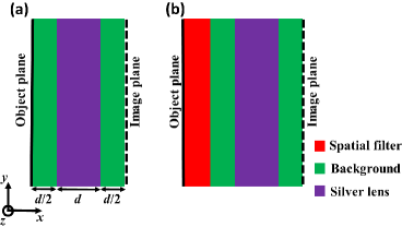
Figure 1: Schematic of a typical silver lens imaging system (a) without ACI and (b) the modified form with the integrated spatial filter for an implementation of ACI. The TM-polarized field distribution on the object plane propagates through each system and is recorded from the image plane. The purple, green, and red regions are the silver lens, background dielectric and the integrated spatial filter, respectively.

In ACI, loss compensation can be performed by introducing an additional material between the object plane and the lens as shown in Fig. 1(b). This material should behave as a tunable active band-pass spatial filter Ghoshroy et al. (2017, 2018b). We write the transfer function of the spatial filter as Ghoshroy et al. (2018a)

$$a(k_{y})=b+G(k_{y}),$$ (1)

where we set $b$ as a real constant corresponding to a uniform low background transmission. $G(k_{y})=|G(k_{y})|\mathrm{e}^{i\varphi(k_{y})}$ is a complex band-limited function with phase $\varphi(k_{y})$ and describes the pass-band of the passive filter. If the amplitude of the wave illuminating the system is increased by a factor $A_{0}=b^{-1}$, the resulting transmitted spectrum is

$$A(k_{y})=1+A_{0}G(k_{y}).$$ (2)

Eq. 2 is defined as the transfer function of the active spatial filter Ghoshroy et al. (2018a). The term “active spatial filter” simply refers to the process of physically providing increased energy to the passive filter with the transfer function in Eq. 1. In other words, linear transmission through passive materials is considered. The word active also distinguishes ACI from purely deconvolution based methods Zhang et al. (2016); Adams et al. (2016); Zhang et al. (2017); Adams et al. (2017) where no additional energy is provided to the system.

The response of the active spatial filter should be shift invariant along the object plane and integrating the filter with the lens should allow the entire system to be described with an active transfer function Ghoshroy et al. (2017, 2018b) written as

$$T_{A}(k_{y})=T(k_{y})[1+A_{0}G(k_{y})],$$ (3)

where $T(k_{y})$ is the passive transfer function of the silver lens.

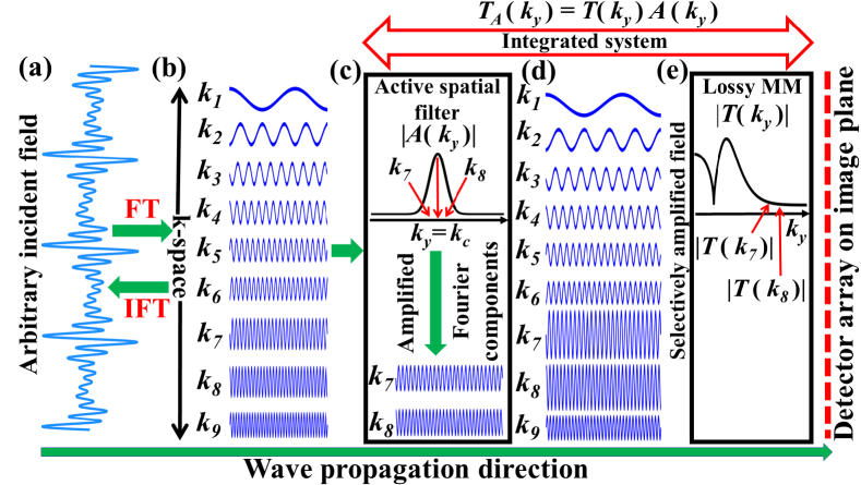
Figure 2: Conceptual schematic of ACI emphasizing the underlying physics of the loss compensation process. (a) An arbitrary incident field is (b) a weighted superposition of different harmonics. After propagating though (c) the active spatial filter, the amplitudes of a few selected harmonics (e.g., $k_{7}$ and $k_{8}$) are amplified relative to the others based on the transfer function of the filter given by Eq. 2 and depicted by the inset in (c). (d) The modified field incident on (e) the lossy MM contain the amplified spatial frequencies (origin of auxiliary source), superimposed with the unaltered harmonics. The estimated amplification provided to the selected harmonics can be the inverse of their passive transmission amplitudes (e.g., $T(k_{7})$ and $T(k_{8})$ in the inset). This would ensure that they survive the lossy transmission process through the MM.

The Eqs. 2 and 3 are central to the ACI loss compensation process. The physical picture is best illustrated with the aid of the schematic shown in Fig. 2. An arbitrary field incident on the system, shown in Fig. 2(a) can be described as a linear, weighted superposition of harmonics or spatial frequencies shown in Fig. 2(b). The active spatial filter in Fig. 2(c) is inserted between the lossy MM in Fig. 2(e) and the incident field. The transfer function of the active filter has the form of Eq. 2 and the amplitude $|A(k_{y})|$ is depicted in the inset in Fig. 2(c). The transmission amplitude of a lossy MM, which deteriorates for increasing spatial frequencies, is illustrated by the inset in Fig. 2(e). For example, assume that the spatial frequencies $k_{7}$ and $k_{8}$ will be compensated. ACI achieves this by tuning the center frequency, $k_{c}$ of the active spatial filter such that $|A(k_{y})|>1$ over the identified spatial frequencies. This is illustrated by the inset in Fig. 2(c). After the harmonics of the incident field propagate though the active spatial filter, the amplitudes of the identified spatial frequencies are amplified relative to the other harmonics. Therefore, the field exiting the active filter contains the original harmonics of the object superimposed with the selectively amplified harmonics $k_{7}$ and $k_{8}$ [see Fig. 2(d)]. The amplification provided to these harmonics (controlled by $A_{0}$) is adjusted to ensure that they survive the lossy transmission process through the MM. The selectively amplified spatial frequencies at the exit of the filter constitute the auxiliary source as discussed in Ghoshroy et al. (2017) and is conceptually similar to Sadatgol et al. (2015) with the only difference being the generation process, which here like in Ghoshroy et al. (2017) employs the active spatial filter to simply modify the original field incident on the MM by a convolution operation.

Using numerical simulations, ACI was implemented with an experimentally realized silver superlens Fang et al. (2005) at the wavelength $\lambda=365\,$nm. A physical system approximating the properties of the active spatial filter was designed with aluminium-dielectric multilayered structures which exhibit hyperbolic dispersion Ghoshroy et al. (2018a). The above theoretical formulation was tested by integrating the multilayered structure with the lens as shown in Fig. 1(b). Imaging results with coherent Ghoshroy et al. (2018b) and incoherent Adams et al. (2018) illumination showed an improvement in the resolution limit of the lens even under the presence of noise. The HMMs used in Ghoshroy et al. (2018b); Adams et al. (2018) were designed to act as the spatial filter in Fig. 1(b), such that their transmission properties closely approximate Eq. 2 under high intensity illumination.

III Variance in the Fourier Domain

To start with, let the image plane has a length $L$ along the y-axis [see Fig. 3(a)]. A continuous signal $i(y)$, along the image planes is measured by a detector which can be an array of pixels or a scanning near-field probe. Based on the setup in Fig. 1, $i(y)$ represents TM-polarized field. An arbitrary spatial field distribution is decomposed into $M$ discrete samples at intervals of $\Delta y$ where $M$ is an even integer. The above spatial decomposition is represented by the segmented line in Fig. 3(a) where each segment is defined as a pixel. An integer $p$ satisfying $-\frac{M}{2}\leq p\leq\frac{M}{2}-1$ uniquely identifies each pixel centered at $y(p)=p\Delta y\equiv\xi$. This relates the discrete space $\xi$ to continuous space $y$. The signal sampled by the $p^{\mathrm{th}}$ pixel is denoted by $i(\xi)$. In subsequent calculations we will set $L=80\lambda$ with $\lambda=365\,$nm and $M=5840$. Therefore, the sampling interval is $\Delta y=5\,$nm which is slightly larger than previously demonstrated apertureless probes which can achieve resolutions down to $1\,$nm Zenhausern et al. (1995). The resulting noisy image at each pixel is described with a popular signal-modulated noise model Heine and Behera (2006); Walkup and Choens (1974); Kasturi et al. (1983); Froehlich et al. (1981); Sadhar and Rajagopalan (2005). The image plane is thought of as an array of statistically independent random variables (RVs) and the subsequent noisy image at the $p^{\mathrm{th}}$ pixel is denoted by

$$i_{n}(\xi)=\bigg{[}|i(\xi)|+n_{sd}(\xi)\bigg{]}\mathrm{e}^{i\theta(\xi)}.$$ (4)

$i(\xi)$ is the noiseless field at the image plane and is corrupted by signal-dependent (SD) noise process $n_{sd}(\xi)$. The discussion of signal-independent noise can be found in Ghoshroy et al. (2017, 2018a). The RV $n_{sd}(\xi)$ in Eq. 4 has zero mean, Gaussian probability density function, and standard deviation $f\{|i(\xi)|\}^{\gamma}\sigma_{sd}$, where $\sigma_{sd}$ is a constant. $\theta(\xi)$ is the phase of the noiseless coherent field $i(\xi)$ at the $p^{\mathrm{th}}$ pixel (i.e., $\xi\equiv p\Delta y$). A correction due to the shift in the zero-optical-path difference point based on an interferometric setup was not included in our model. $f\{|i(\xi)|\}^{\gamma}$ is a function of the ideal image amplitude and is referred to as the modulation function Heine and Behera (2006). $\gamma$ is a parameter satisfying $0\leq\gamma\leq 1$ Walkup and Choens (1974). The variance at each pixel is,

$$\sigma_{\xi_{p}}^{2}=f\{|i(\xi)|\}^{2\gamma}\sigma_{sd}^{2}.$$ (5)

The modulation function and the value of $\gamma$ are selected to best mimic the behavior of SD noise which affects the system.

The above detection process results in a similar decomposition of the continuous Fourier spectrum of $i(y)$ into $M$ discrete spatial frequencies as illustrated by the segmented line in Fig. 3(b). Two adjacent frequencies are separated by $\Delta k_{y}$ and the individual spatial frequencies are referenced by $k_{y}(q)=q\Delta k_{y}\equiv\zeta$, where $-\frac{M}{2}\leq q\leq\frac{M}{2}-1$. This relates the discrete Fourier space $\zeta$ to continuous Fourier space $k_{y}$. The Fourier transform of the discretized noise-free image, $i(\xi)$, is denoted by $I(\zeta)$, and the standard deviation at the $q^{\mathrm{th}}$ spatial frequency is $\sigma_{\zeta_{q}}$. Knowledge of $\sigma_{\zeta_{q}}$ is particularly useful in determining the maximum achievable limiting resolution for optical systems where transmission progressively worsens for high spatial frequencies. For example, the Fourier components with transmitted amplitudes comparable to, or less than $\sigma_{\zeta_{q}}$ will be indiscernible from random noise fluctuations within the measured signal. Therefore, $\sigma_{\zeta_{q}}$ allows us to identify the spatial frequencies whose Fourier domain information is effectively lost due to noise effects. Additionally, the effectiveness of a loss compensation technique can also be evaluated by monitoring its effect on $\sigma_{\zeta_{q}}$. Thus, a formulation of $\sigma_{\zeta_{q}}$ is important for our understanding of the underlying mechanism of ACI and its capacity at compensating losses while minimizing noise amplification.

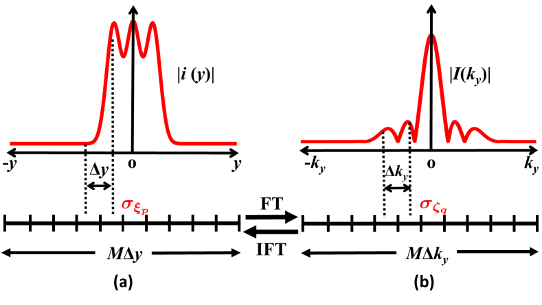
Figure 3: Illustration of an image measurement process in a detector system. (a) The continuous field $i(y)$ along the image plane of length $L$ is decomposed into $M$ samples at intervals of $\Delta y$. Each sample is identified by an integer $p$. During the detection process, noise degrades the ideal image and the standard deviation at each sample is $\sigma_{\xi_{p}}$.$|i_{n}(\xi)|$ is the magnitude of the recorded image at the $p^{\mathrm{th}}$ pixel or $y=p\Delta y\equiv\xi$ spatial coordinate. (b) The Fourier spectrum of $i(\xi)$ is similarly a decomposition into $M$ spatial frequencies and $\sigma_{\zeta_{q}}$ is the standard deviation at the $q^{\mathrm{th}}$ frequency.

A general expression for the standard deviation at the $q^{\mathrm{th}}$ spatial frequency can be calculated by approximating the analytical Fourier transform relation as a Riemann sum Voelz (2011). The Fourier transform of the noisy image $i_{n}(\xi)$ in Eq. 4 is then written as

$$I_{n}(\zeta) ={\sum\limits^{(\frac{M}{2}-1)\Delta y}_{\xi=-\frac{M}{2}\Delta y}}|i_{n}(\xi)|\mathrm{e}^{i\theta(\xi)}\exp\bigg{(}-{i\xi\zeta}\bigg{)}\Delta y$$

$$={\sum\limits^{(\frac{M}{2}-1)\Delta y}_{\xi=-\frac{M}{2}\Delta y}}|i_{n}(\xi)|\bigg{\{}\cos\bigg{(}\theta(\xi)-{\xi\zeta}\bigg{)}$$

$$+i\sin\bigg{(}\theta(\xi)-{\xi\zeta}\bigg{)}\bigg{\}}\Delta y$$

$$=I^{\prime}_{n}(\zeta)+iI^{\prime\prime}_{n}(\zeta)$$ (6)

with real and imaginary parts $I^{\prime}_{n}(\zeta)$ and $I^{\prime\prime}_{n}(\zeta)$, respectively. Note that the number of samples $M$, is related to $\Delta y$ and $\Delta k_{y}$ by $M=2\pi/\Delta y\Delta k_{y}$ Voelz (2011). We can substitute $|i_{n}(\xi)|$ from Eq. 4 into Eq. 6 to express the real and imaginary parts of $I_{n}(\zeta)$ as

$$I^{\prime}_{n}(\zeta)={\sum\limits^{(\frac{M}{2}-1)\Delta y}_{\xi=-\frac{M}{2}\Delta y}}\bigg{\{}|i(\xi)|+n_{sd}(\xi)\bigg{\}}\cos[\phi(\xi,\zeta)]\Delta y,$$ (7)

and

$$I^{\prime\prime}_{n}(\zeta)={\sum\limits^{(\frac{M}{2}-1)\Delta y}_{\xi=-\frac{M}{2}\Delta y}}\bigg{\{}|i(\xi)|+n_{sd}(\xi)\bigg{\}}\sin[\phi(\xi,\zeta)]\Delta y,$$ (8)

respectively, and $\phi(\xi,\zeta)={\theta(\xi)-\xi\zeta}$.

Based on Eq. 6, we can write $I_{n}(\zeta)$ as

$$I_{n}(\zeta)=I(\zeta)+N_{sd}(\zeta),$$ (9)

where $I(\zeta)$ and $N_{sd}(\zeta)$ are the Fourier transforms of $i(\xi)$ and $n_{sd}(\xi)$ in Eq. 4, respectively. The real and imaginary parts of $I(\zeta)$ and $N_{sd}(\zeta)$ can also be expressed in terms of the sums of cosines and sines similar to $I_{n}(\zeta)$ (see Eqs. 7 and 8). $N_{sd}(\zeta)$ in Eq. 9 has a standard deviation $\sigma_{\zeta_{q}}$ describing SD noise at the $q^{\mathrm{th}}$ Fourier component. The variance of the real and imaginary parts of $N_{sd}(\zeta)$ are denoted by $\sigma^{2}_{\zeta_{q},r}$ and $\sigma^{2}_{\zeta_{q},i}$, respectively. According to Eqs. 6 and 9 $N_{sd}(\zeta)$ is a weighted superposition of all the RVs in the spatial domain. Each RV involved in the summation is statistically independent with a Gaussian probability density function. Therefore, we can apply Bienaymé’s identity, to express $\sigma^{2}_{\zeta_{q},r}$ and $\sigma^{2}_{\zeta_{q},i}$ as

$$\sigma^{2}_{\zeta_{q},r}={\sum\limits^{(\frac{M}{2}-1)\Delta y}_{\xi=-\frac{M}{2}\Delta y}}\sigma^{2}_{\xi_{p}}\cos^{2}[\phi(\xi,\zeta)](\Delta y)^{2},$$ (10)

and

$$\sigma^{2}_{\zeta_{q},i}={\sum\limits^{(\frac{M}{2}-1)\Delta y}_{\xi=-\frac{M}{2}\Delta y}}\sigma^{2}_{\xi_{p}}\sin^{2}[\phi(\xi,\zeta)](\Delta y)^{2},$$ (11)

respectively, and $\sigma^{2}_{\xi_{p}}=f\{|i(\xi)|\}^{2\gamma}\sigma^{2}_{sd}$. The overall variance at each spatial frequency is simply the sum of the variances of the real and imaginary parts in Eqs. 10 and 11, that is

$$\sigma_{\zeta_{q}}^{2}={\sum\limits^{(\frac{M}{2}-1)\Delta y}_{\xi=-\frac{M}{2}\Delta y}}f\{|i(\xi)|\}^{2\gamma}\sigma_{sd}^{2}(\Delta y)^{2}.$$ (12)

Without loss of generality, the subsequent calculations can be simplified and provide more physical insight by assuming the modulation function in Eq. 12 is a linear function of $|i(\xi)|$ with $\gamma=1$. This results in constant SNR and has implications on the considered noise levels and required illumination intensities. This is chosen to relate the variance directly to the total physical power contained in the signal as shown below. Similar effects are obtained, such as in practical detectors with the Poisson distribution of photon noise Adams et al. (2018); Heine and Behera (2006); Adams (2019). Substituting $f\{|i(\xi)|\}=|i(\xi)|$ and $\gamma=1$ we can rewrite Eq. 12 as

$$\sigma_{\zeta_{q}}^{2}=\bigg{[}{\sum\limits^{(\frac{M}{2}-1)\Delta y}_{\xi=-\frac{M}{2}\Delta y}}|i(\xi)|^{2}\sigma_{sd}^{2}\Delta y\bigg{]}\Delta y.$$ (13)

The summation enclosed inside brackets, is proportional to the optical power on the image plane. Therefore, we can employ the energy conservation theorem by using Parseval’s relation and rewrite $\sigma_{\zeta_{q}}^{2}$ in Eq. 13 as

$$\sigma_{\zeta_{q}}^{2} =\bigg{[}\frac{1}{2\pi}{\sum\limits^{(\frac{M}{2}-1)\Delta k_{y}}_{\zeta=-\frac{M}{2}\Delta k_{y}}}{|I(\zeta)|}^{2}\sigma_{sd}^{2}\Delta k_{y}\bigg{]}\Delta y$$

$$=\frac{1}{M}{\sum\limits^{(\frac{M}{2}-1)\Delta k_{y}}_{\zeta=-\frac{M}{2}\Delta k_{y}}}{|I(\zeta)|}^{2}\sigma_{sd}^{2}.$$ (14)

Eqs. 13 and 14 state, for a fixed number of pixels $M=2\pi/\Delta y\Delta k_{y}$, that the spectral variance $\sigma_{\zeta_{q}}^{2}$ is constant and proportional to the total power contained in the signal. Similar results have been reported for incoherent light in Ingerman et al. (2019); Becker et al. (2018); Lucke (2001). This is a remarkable result, which can be potentially generalized to a wide variety of problems in noisy and lossy linear systems, either classical or quantum. Below, in the context of superresolution imaging, we demonstrate how this result leads to enhanced spectral SNR with the incorporation of selective spectral amplification and correlations. For different values of $\gamma$, the variance is still flat, but not proportional to the power contained in the signal (see Eq. 12). To the best of our knowledge, the utilization of Eqs. 13 and 14 in imaging has only been drawn attention to here and in a slightly modified form recently in Becker et al. (2018) to extend the SNR limit using sub-pupils.

The presence of an extra $\Delta y$ clearly makes $\sigma_{\zeta_{q}}^{2}$ dependent on the spatial discretization. Rescaling $\Delta y$ in Eq. 14 would result in effects of upsampling or downsampling of continuous signals. Therefore, Eq. 14 cannot be readily generalized for an arbitrary detector system without considering the physical mechanism through which information is extracted. The spectral variance may not necessarily reduce with pixel miniaturization and multiple factors must also be considered when determining the overall effect on noise. The number of detected photons are also intimately related to the pixel active area, quantum efficiency, the pixel optical path, integration time, and sensitivity Agranov et al. (2007); Bigas et al. (2006); Shcherback and Yadid-Pecht (2003); Mitrofanov et al. (2001). Additionally, it may be necessary to incorporate crosstalk effects between adjacent pixels to accurately model the effect of pixel scaling on $\sigma_{\zeta_{q}}^{2}$. However, the effects of pixel miniaturization on the detected noise are considered independent from ACI, which only deals with compensation of signal losses for a fixed number of pixels.

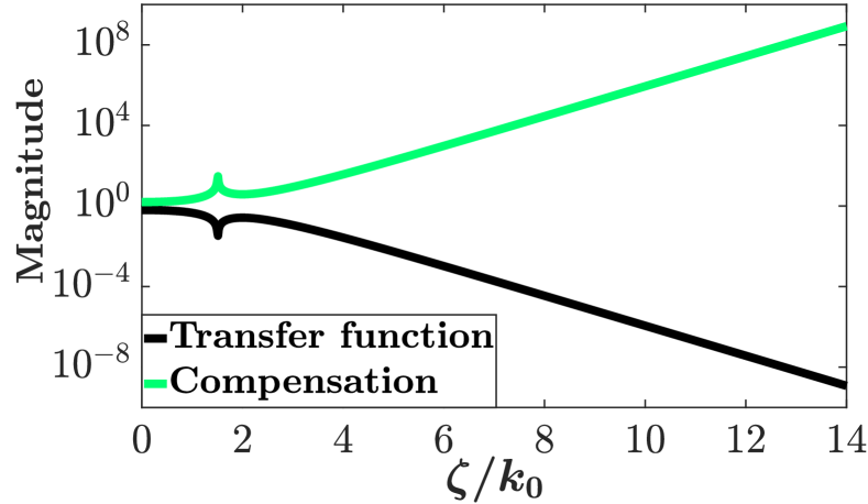
Figure 4: Magnitude of the analytical transfer function for a $50\,$nm thick silver lens embedded inside a dielectric and symmetrically placed between the object and image planes as shown in Fig. 1(a). The required compensation at each Fourier component should ideally be the inverse of the transfer function and is shown by the green line.

In subsequent discussions, an analytical equation Fang et al. (2003) is used for the transfer function of the silver lens imaging system, which is configured similar to an experimental silver lens Fang et al. (2005) with $d=50\,$nm and embedded inside a background dielectric of relative permittivity $\epsilon_{d}=2.5$ Ghoshroy et al. (2018a, b); Adams et al. (2018) [see Figs. 1(a) and 4]. The relative permittivity of silver at $\lambda=365\,$nm is $\epsilon_{Ag}=-1.88+0.60i$, calculated from the Drude-Lorentz model Rakić et al. (1998). The corresponding estimated compensation necessary for each spatial frequency is simply the inverse of the corresponding magnitude of transmission (see Fig. 4). In Fig. 4 and following ones negative spatial frequencies are not shown, although the full spectrum is considered in all the calculations.

IV Results

IV.1 Selective spectral amplification and correlations

In the following, an example object with a Gaussian spectrum is employed in Figs. 5 and 6, defined as

$$|O(\zeta)|=\exp\bigg{[}\frac{-\zeta^{2}}{2\alpha^{2}}\bigg{]},$$ (15)

where $\alpha$ describes the full width at half maximum (FWHM) of $|O(\zeta)|$ and is defined as

$$\alpha=\frac{0.25M\Delta k_{y}}{2\sqrt{2\ln 2}}.$$ (16)

The imaging systems are illuminated with a TM-polarized source from the object plane (see Fig. 1). We assume that the object field is created through subwavelength slits Taubner et al. (2006); Liu et al. (2007). The spatially coherent discretized complex magnetic field distribution along the object plane is denoted as $o(\xi)$. The Fourier transforms of the noiseless image for the passive (i.e., without ACI) and active (i.e., with ACI) imaging systems are

$$I_{P}(\zeta)=O(\zeta)T(\zeta),$$ (17a)

$$I_{A}(\zeta)=O(\zeta)T(\zeta)[1+A_{0}G(\zeta)],$$ (17b)

respectively, where $O(\zeta)=\mathcal{F}\{o(\xi)\}$ and $\mathcal{F}$ is the Fourier transform operator. The subscripts “$P$” and “$A$” refer to the passive and active imaging systems, respectively. $O(\zeta)A_{0}G(\zeta)$ in Eq. 17b is defined as the auxiliary source Ghoshroy et al. (2017, 2018a, 2018b) (see Fig. 2). Therefore, $O(\zeta)T(\zeta)A_{0}G(\zeta)$ is the residual auxiliary source which survived the lossy transmission process through the lens. As can be seen from Eq. 17b, the object field $O(\zeta)$ is superimposed coherently with the auxiliary source. The auxiliary source is required to possess three important properties. First, it is correlated with the object field $O(\zeta)$ Ghoshroy et al. (2017). Second, it is defined over a finite bandwidth through $G(\zeta)$. Third, it is amplified by a factor of $A_{0}$. Below, without loss of generality, we use a band-limited unit magnitude rectangular function for $G(\zeta)$. Then, overall, the auxiliary source corresponds to only a portion of the object spectrum, which is selectively amplified. However, in general, the function $G(\zeta)$ can have an arbitrary profile with a finite bandwidth Ghoshroy et al. (2018a). In this case, the auxiliary source spectrum is modified in accordance with the given function $G(\zeta)$, while being still selectively amplified and correlated with the object. In Ghoshroy et al. (2018a) and Ghoshroy et al. (2018b), we show how to construct such an auxiliary source using HMMs acting as near-field spatial filters.

The standard deviations at the $q^{\mathrm{th}}$ Fourier component corresponding to $I_{P}(\zeta)$ and $I_{A}(\zeta)$ in Eq. 17 are denoted by ${\sigma_{\zeta_{q},P}}$ and ${\sigma_{\zeta_{q},A}}$, respectively. Their expressions are determined by substituting $|I(\zeta)|$ in Eq. 14 with $|I_{P}(\zeta)|$ and $|I_{A}(\zeta)|$, respectively. That is

$$\sigma^{2}_{\zeta_{q},P}=\frac{1}{M}{\sum\limits^{(\frac{M}{2}-1)\Delta k_{y}}_{\zeta=-\frac{M}{2}\Delta k_{y}}}|O(\zeta)T(\zeta)|^{2}\sigma_{sd}^{2},$$ (18)

and

$$\sigma^{2}_{\zeta_{q},A} =\frac{1}{M}{\sum\limits^{(\frac{M}{2}-1)\Delta k_{y}}_{\zeta=-\frac{M}{2}\Delta k_{y}}}|O(\zeta)T(\zeta)|^{2}\sigma_{sd}^{2}|1+A_{0}G(\zeta)|^{2}$$

$$=\sigma^{2}_{\zeta_{q},P}+\sigma^{2}_{\zeta_{q},Aux}.$$ (19)

Note that $\sigma^{2}_{\zeta_{q},A}$ can be split into its contributing parts. $\sigma^{2}_{\zeta_{q},Aux}$ describes the contribution to the SD noise from the residual auxiliary source and is given by

$$\sigma^{2}_{\zeta_{q},Aux} =\frac{1}{M}{\sum\limits^{(\frac{M}{2}-1)\Delta k_{y}}_{\zeta=-\frac{M}{2}\Delta k_{y}}}|O(\zeta)T(\zeta)|^{2}A_{0}^{2}\sigma_{sd}^{2}$$

$$\times\bigg{[}\frac{2G^{\prime}(\zeta)}{A_{0}}+|G(\zeta)|^{2}\bigg{]},$$ (20)

where $G^{\prime}(\zeta)$ is the real part. Eqs. 18 and 19, say that integrating the active spatial filter with the imaging system gives an additional standard deviation $\sigma_{\zeta_{q},Aux}$, dependent on the filter parameters. Eq. 20 shows how the active filter parameters, such as $A_{0}$, the center frequency $q_{c}$, and the width of $G(\zeta)$ contribute to the noise at each Fourier component. Before proceeding further, we reduce Eq. 20 to

$$\sigma^{2}_{\zeta_{q},Aux}\approx\frac{1}{M}{\sum\limits^{(\frac{M}{2}-1)\Delta k_{y}}_{\zeta=-\frac{M}{2}\Delta k_{y}}}|O(\zeta)T(\zeta)|^{2}A_{0}^{2}\sigma_{sd}^{2}|G(\zeta)|^{2},$$ (21)

since the summation of the first term inside the brackets in Eq. 20 can be generally dropped. For example, consider compensating the spatial frequencies $10k_{0}\leq\zeta\leq 12k_{0}$. According to the green line in Fig. 4, the estimated value for $A_{0}$ is approximately within the order $10^{6}\sim 10^{8}$.

For simplicity, we rewrite the transfer function of the active spatial filter in Eq. 2 as

$$A_{R}(\zeta)=1+A_{0}G_{R}(\zeta),$$ (22)

where $G_{R}(\zeta)=|G_{R}(\zeta)|\mathrm{e}^{i\varphi_{R}(\zeta)}$ is a unit magnitude rectangular function of width $Wk_{0}$ and centered at $\zeta_{c}$. That is

$$|G_{R}(\zeta)|=\left\{\begin{array}[]{cr}1&\hskip 14.22636pt\bigg{|}\frac{(\zeta-\zeta_{c})}{Wk_{0}}\bigg{|}\leq\frac{1}{2}\\ 0&\hskip 14.22636pt\texttt{otherwise}.\\ \end{array}\right.$$ (23)

This redefinition conveniently emphasizes the effect of selective spectral amplification without loss of generality. Then, we can express the ratio $R_{\sigma}$ of $\sigma^{2}_{\zeta_{q},Aux}$ in Eq. 21 to $\sigma^{2}_{\zeta_{q},P}$ in Eq. 18 as

$$R_{\sigma}=A_{0}^{2}\frac{P_{I_{P},W}}{P_{I_{P}}},$$ (24)

where $P_{I_{P},W}$ is the portion of the total power contained by $I_{P}(\zeta)$ distributed over bandwidth $Wk_{0}$ and centered at $\zeta_{c}$, and $P_{I_{P}}$ is the total power contained by $I_{P}(\zeta)$. Thus, it is important to note that Eq. 24 is the ratio of the power in the selectively amplified band to the total power in the noiseless signal without selective amplification. This ratio should not be too large to prevent excessive noise amplification.

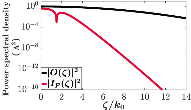
Figure 5: The power spectral densities of the object ($|O(\zeta)|^{2}$) and the passive image ($|I_{P}(\zeta)|^{2}$) showing how the total power contained within the Gaussian object and image is distributed throughout the Fourier spectrum.

Consider, for example, the case where the Fourier components within $6k_{0}\leq\zeta\leq 8k_{0}$ are selected for amplification. We set $A_{0}=10^{4}$ to guarantee the recovery of this entire band. This overcompensates the lower spatial frequencies within the band. From Eq. 24 the ratio $R_{\sigma}$ evaluates to about $13$. This indicates that even though Fourier components were strongly amplified, the resultant increment in the spectral variance is comparatively small. This can be generalized for an arbitrary $\zeta_{c}$. Fig. 5 shows the power spectral density (PSD) plots for $|O(\zeta)|^{2}$ and the corresponding $|I_{P}(\zeta)|^{2}=|O(\zeta)T(\zeta)|^{2}$ indicated by black and red lines, respectively. Since $|T(\zeta)|$ decays with increasing $q$ (see black line in Fig. 4), the PSD of $I_{P}(\zeta)$ clearly follows a similar trend. Most of the power contained within the image is distributed over a small portion of the Fourier spectrum. For example, if the previously selected band is modified to $8k_{0}\leq\zeta\leq 10k_{0}$, $P_{I_{P},W}$ in Eq. 24 will decrease as can be seen from Fig. 5. However, $P_{I_{P}}$ will remain the same and therefore, the ratio between $P_{I_{P},W}$ and $P_{I_{P}}$ decreases. This conveniently restricts $R_{\sigma}$ from becoming large even though the Fourier components within $8k_{0}\leq\zeta\leq 10k_{0}$ require larger amplification compared to the previous example.

Based on $R_{\sigma}$ in Eq. 24 the ACI technique suggests, in principle, an infinite resolution. Because there is a trade-off between the illumination intensity and the bandwidth of the passive spatial filter to keep the spectral SNR above $0\,$dB at an arbitrarily large spatial frequency in the loss compensated image spectrum. Once the SNR is above $0\,$dB for a particular spatial frequency, that particular frequency of the image can be reconstructed with deconvolution using the active transfer function in Eq. 3. The larger the illumination intensity, the smaller the bandwidth should be to suppress the noise amplification. However, in practice the resolution is limited by several factors: maximum power, minimum bandwidth and maximum center frequency of the passive spatial filter, and the minimum pixel size. Also, the present model of ACI does not consider weak signals, which should be treated with a quantum optical model Haus (2012).

IV.2 Improving SNR and resolution limits

The above inhibition of noise amplification during the compensation process results in substantial improvement in system performance Ghoshroy et al. (2017, 2018b); Adams et al. (2018). This is investigated by comparing between the spectral SNR of the passive and active systems. A general expression for the spectral SNR is

$$SNR(\zeta)=\frac{|I(\zeta)|}{\sigma_{\zeta_{q}}}.$$ (25)

Substituting the constant $A_{0}$ with a functional form $A_{0}(\zeta)=|T(\zeta)|^{-1}$ allows optimal amplification for full compensation of losses within $Wk_{0}$ bandwidth and is adopted below to emphasize the relative importance of the selective amplification rather than the exact functional form. Alternatively, a Gaussian or log-normal form of $|G_{R}(\zeta)|$ can also be used to better describe the previously considered MM spatial filters Ghoshroy et al. (2018a, b). Additionally, for the remainder of this work we will use $\sigma_{sd}=10^{-3}$ in the signal-modulated noise model in Eq. 4 for consistency with our previous works Ghoshroy et al. (2017, 2018a, 2018b); Adams et al. (2018), where an experimental imaging system detector Akiba et al. (2010) is considered.

Based on Eqs. 17 and 25, the SNR of the passive and active imaging systems $SNR_{P}(\zeta)$ and $SNR_{A}(\zeta)$, respectively, are written as

$$SNR_{P}(\zeta)=\frac{|O(\zeta)T(\zeta)|}{\sigma_{\zeta_{q},P}},$$ (26)

and

$$SNR_{A}(\zeta)=\frac{|O(\zeta)T(\zeta)||1+A_{0}(\zeta)G_{R}(\zeta)|}{\sigma_{\zeta_{q},A}},$$ (27)

respectively. $SNR_{P}(\zeta)$ is plotted by the black line in Fig. 6 and $SNR_{A}(\zeta)$ for filters with $W=1,3,4$, and $6$ by the pink, green, blue and purple lines, respectively. Note that $\zeta_{c}$ is kept constant at $10k_{0}$ and the dashed yellow line marks $SNR=0\,$dB. The intersection of $SNR_{P}(\zeta)$ with the dashed line marks the resolution limit of the passive system since larger Fourier components will be indistinguishable from noise in the detected signal. However, $SNR_{A}(\zeta)$ shows a remarkable improvement especially within the regions where compensation is provided. We point out that $SNR_{A}(\zeta)$ is less than $SNR_{P}(\zeta)$ outside the selected bands as expected, since the additional noise from $\sigma_{\zeta_{q},Aux}$ affects the entire spectrum (see Eq. 14). This contribution increases with $W$ as is evident from Fig. 6. Nevertheless, the additional increment in the spectral variance is significantly smaller than the amplification provided to each Fourier components inside the selected bands, which results in an impressive enhancement in SNR. The purple line is particularly interesting since it encapsulates the remarkable power of ACI. The rectangle function $|G_{R}(\zeta)|$, in this case, spans a fairly broad $6k_{0}$ bandwidth and has essentially extended the resolution limit of the system close to double compared to the passive system.

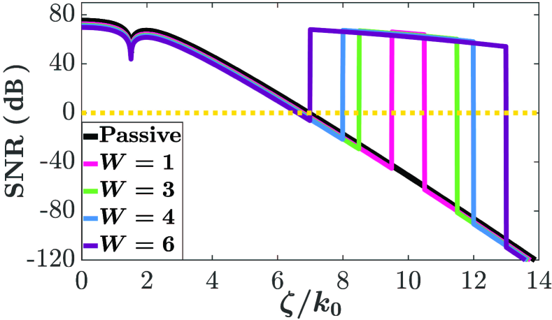
Figure 6: SNRs of the passive (black line) and active imaging systems (pink, green, blue and purple lines) with different $W$. The effective resolution limit of the passive imaging system is approximately $\zeta=7k_{0}$. In contrast, the SNR of the active imaging systems incorporating ACI is increased within the selected bands of each filter. Slightly reduced SNR outside the selected bands indicate the noise contribution from the auxiliary source.

IV.3 Arbitrary objects

In general, the theory of ACI can be expanded to arbitrary objects. This is illustrated with Fig. 7 where the Fourier spectrum of an arbitrary object is plotted by the black line. The corresponding noise-free passive image spectrum is calculated from Eq. 17a and corrupted with noise in the spatial domain according to the signal-modulated noise model in Eq. 4. The noisy image is then Fourier transformed to obtain $I_{n,P}(\zeta)$. The magnitudes of $I_{P}(\zeta)$ and $I_{n,P}(\zeta)$ are shown in Fig. 7 by pink and light green lines, respectively. The standard deviation $\sigma_{\zeta_{q},P}$, which has degraded the passive image spectrum is shown by the dashed dark green line. We can see how $|I_{P}(\zeta)|$ progressively worsens with increasing $\zeta$. Eventually, $\sigma_{\zeta_{q},P}$ becomes comparable to $|I_{P}(\zeta)|$ at approximately $\zeta=7k_{0}$ after which $|I_{n,P}(\zeta)|$ is overwhelmed by noise, similar to the simpler Gaussian object in Fig. 6 (see black line). The noise-free active image spectrum is calculated from Eq. 17b taking $\zeta_{c}=10k_{0}$, $W=4$, and substituting $A_{0}G(\zeta)$ with $A_{0}(\zeta)G_{R}(\zeta)$, where $A_{0}(\zeta)=|T(\zeta)|^{-1}$. This active image is then also corrupted with noise in the spatial domain and Fourier transformed to obtain $I_{n,A}(\zeta)$, magnitude of which is shown by the light blue line in Fig. 7. The standard deviation for the active system $\sigma_{\zeta_{q},A}$ is shown by the dashed dark blue line.

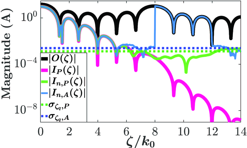
Figure 7: Generalization of the ACI to an arbitrary object. The amplitude of the Fourier transforms of the object, the corresponding noise-free and noisy passive images, and the active image are shown by the black, pink, light green and light blue lines, respectively. The standard deviations for the noisy passive image and the active image spectra are shown by the dashed dark green and dark blue lines, respectively. The active image is adequately compensated within $8k_{0}\leq\zeta\leq 12k_{0}$ with a very small amplification of SD noise.

Fig. 7 clearly manifests the noise-resistant effect of the selective amplification. Note that the missing nodes on the object spectrum are accurately recovered inside the band $8k_{0}\leq\zeta\leq 12k_{0}$ where the selective amplification is provided. The inhibition of noise amplification with ACI’s selective spectral amplification is therefore applicable for arbitrary objects. Based on Fig. 7, we find that the resolution limit can be in the end extended by more than $40\,\%$ when the underlying passive spatial filter is illuminated with an intensity of about $0.03\mathrm{mW/\upmu m^{2}}$ (i.e., the intensity amplification factor $A_{0}^{2}\approx 1.6\times 10^{5}$). A coherent light around this level of intensity is accessible for a superresolution imaging experiment with a relatively less lossy MM structure Liu . Retrieving deep subwavelength information from a low-Q system disturbs the system and lets the high spatial frequency modes quickly dissipate. In our calculations we did not include this effect. Therefore, it is necessary to maintain a sufficiently high intensity continuous wave illumination to counter this effect. Here, for simplicity, we consider only one-dimensional imaging. Therefore, the dimension of the pixel along the $z$-direction can be taken equal to the length $L$ of the image plane. For two-dimensional imaging more intensity is needed. Additional noise and speckle associated with high illumination intensity and small pixel size limit the achievable resolution. Also, the amplification at high spatial frequencies will be difficult in the presence of spatial dispersion. Therefore, the designed spatial filter in Fig. 1(b) should support the highest desired spatial frequency. In a future work, an efficient (i.e., low power) implementation could replace the spatial filter in Fig. 1(b) with a plasmonic structured illumination Bezryadina et al. (2018) that is systematically designed based on Eqs. 13 and 14. Another possibility could be considered along the lines of Xiong et al. (2007), where the HMM is used to collect the low and high spatial frequencies at different polarizations. In our model, we assume $60\,$dB spatial SNR (i.e., $\sigma_{sd}=10^{-3}$). Since the spectral variance is constant through the image spectrum (see Fig. 7) and proportional to $\sigma_{sd}^{2}$, the larger the spatial SNR the lower the required power is to reconstruct a specific spatial frequency.

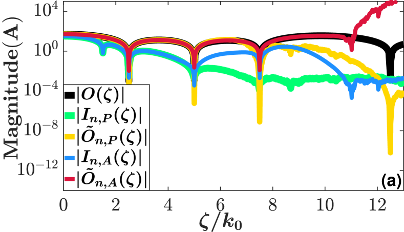
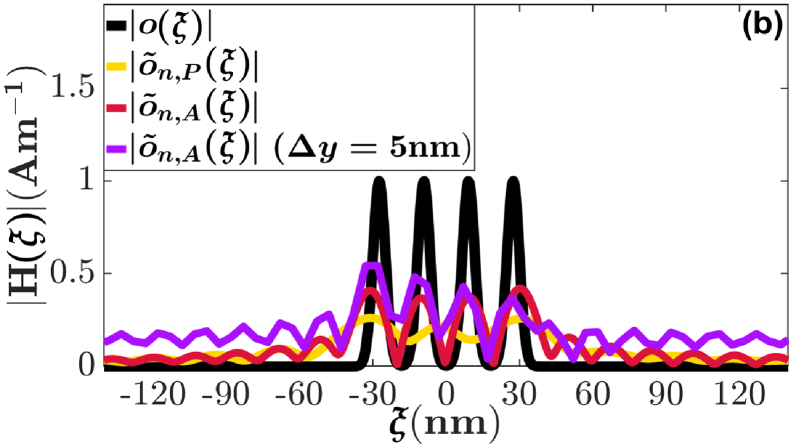
Figure 8: The comparison of the image reconstruction using ACI (without optimal Wiener filter) and the passive image reconstruction using the optimal Wiener filter, in (a) Fourier domain and (b) spatial domain. $\tilde{O}_{n,P}(\zeta)$ and $\tilde{O}_{n,A}(\zeta)$ refer to passive reconstructed image spectrum obtained by the optimal Wiener filter and the active reconstructed image spectrum obtained by the ACI without optimal Wiener filter. $\tilde{o}_{n,P}(\xi)$ and $\tilde{o}_{n,A}(\xi)$ are the respective reconstructed images in the spatial domain. The object (black) and the noisy images $\tilde{I}_{n,P}(\zeta)$ and $\tilde{I}_{n,A}(\zeta)$ before deconvolution are also indicated. Only magnitudes are shown. In (b) the discrete space $\xi$ is interpolated to guide the eye. The ACI method clearly resolves the 4 objects (see black lines) separated by $18\,$nm peak-to-peak distance, using 2 overlapping Gaussian pass-bands with FWHMs of $2.3k_{0}$ and centered at $7k_{0}$ and $8.5k_{0}$. The constant amplitude amplification factor $A_{0}=630$.

In the ACI method, once the selective amplification is applied to the spatial frequencies that were previously buried under the noise (see Fig. 7), the reconstructed image can be obtained from deconvolution based on the active transfer function (see Eq. 3). If the optimal Wiener filter $[1+1/SNR_{A}(\zeta)^{2}]^{-1}$ Roggemann et al. (1992); Biemond et al. (1990); Zaknich (2005) is used in the deconvolution step, the reconstructed image can be written as

$$\tilde{O}_{n,A}(\zeta) =I_{n,A}(\zeta)\frac{1}{1+\frac{1}{{SNR_{A}(\zeta)}^{2}}}$$

$$\times\frac{1}{T(\zeta)[1+A_{0}G(\zeta)]},$$ (28)

assuming a constant $A_{0}$ and general pass-band function $G(\zeta)$. For high $SNR_{A}(\zeta)$ (i.e., around low spatial frequencies and regions of selective amplification), this deconvolution process approaches to “active inverse filtering.” For low $SNR_{A}(\zeta)$ (e.g., around $7k_{0}$ and $13k_{0}$ in Fig. 7), the optimal Wiener filter does not heavily amplify the noise as opposed to the inverse filter Roggemann et al. (1992). In general, the optimal Wiener filter employs the image SNR (see Eq. 28) to prevent excessive noise amplification Biemond et al. (1990); Zaknich (2005). In this regard, the selective amplification in the ACI method has also a similar spirit as the optimal Wiener filter. However, as shown below in Fig. 8, with the ACI even without the optimal Wiener filter one can restore spatial frequencies that cannot be restored by a typical optimal Wiener deconvolution Roggemann et al. (1992); Biemond et al. (1990); Zaknich (2005). This is achieved by selectively amplifying those spatial frequencies, while preventing excessive noise amplification in accordance with Eqs. 13 and 14. Furthermore, as given in Eq. 28, when the optimal Wiener filter is integrated with the ACI, this extends the restored spatial frequency range of the optimal Wiener filter.

Fig. 8 compares the passive and active reconstructed images and their corresponding spectra for 4 Gaussian objects separated by $18\,$nm peak-to-peak distance. The yellow line corresponds to the unresolved passive image reconstructed with the optimal Wiener filter. The images reconstructed with the ACI are shown with the red and purple lines in Fig. 8(b). The purple line highlights the effect of discretization assuming $\Delta y=5\,$nm. Consistent with Eq. 14, the noise is increased with larger discretization. It is clearly seen that the objects are fully resolved using ACI, with a resolution better than $\lambda/20$. The selective amplification process of ACI is achieved by 2 overlapping Gaussian pass-bands with FWHMs of $2.3k_{0}$ and centered at $7k_{0}$ (i.e., near the resolution limit of the passive system) and $8.5k_{0}$. The incident plane wave illumination amplitude [see Fig. 1(b)] is increased by a constant factor of $A_{0}=630$. Finally, the reconstructed images are obtained from deconvolution based on the active transfer function (see Eq. 3) and using the noisy active image spectrum $I_{n,A}(\zeta)$ [see blue line in Fig. 8(a)].

V Discussion and Conclusion

The ACI is more than a loss compensation in MMs or plasmonics. The ACI concept, the then-called $\Pi$ scheme, was first numerically demonstrated as a loss compensation method in a plasmonic NIM Sadatgol et al. (2015), but later rapidly evolved into a scheme for the mitigation of information loss in noisy and lossy linear systems. The ACI has, since, turned into a scheme for spectrum manipulation using selective amplification and correlations Ghoshroy et al. (2017, 2018b); Adams et al. (2018).

In this work, we have presented a mathematical analysis of the conceptual framework of ACI. We showed that selective amplification of a controllable band of spatial frequencies with an auxiliary source can provide sufficient amplification to previously attenuated spatial frequencies with minimal amplification of noise. It is important to emphasize that the amplification process in the theory of ACI described here is fundamentally different than the traditional optical gain media and does not require a quantum optical model. The ACI is more feasible than optical gain or nonlinear media, which are more complex and cumbersome due to pumping, gain saturation, or amplified spontaneous emission (ASE) Prasad (1994); Haus (2012). In the coherent model of ACI, the amplification of the spatial frequencies within the selected band (see Figs. 6 and 7) is achieved by the coherent superposition of the original object field with an external auxiliary source, which is correlated with the object field (see Eq. 17). Possible physical generations of the auxiliary source relying on the HMMs and injection of plasmons have been studied in detail in our previous works Sadatgol et al. (2015); Ghoshroy et al. (2018a, b). The implementations for far-field imaging can be made possible with, for example, structured illumination Ingerman et al. (2019) and spatial filtering Becker et al. (2018); Adams (2019). Thus, the ACI does not suffer from the severe adverse effect of ASE on the SNR associated with the amplification of weak signals using optical gain media Prasad (1994); Haus (2012). Also, the imaging system here employs amplification (e.g., by using a brighter source) prior to the lossy transmission to avoid the difficulty with the signal amplification at the detection side, especially for the retrieval of higher spatial frequencies, and is operated with stronger signals. Moreover, the classical correlations play an important role in ACI Ghoshroy et al. (2017); Qian et al. (2017). In practice, the ACI may not necessarily need increased input power or a separate auxiliary source, but may only need to locally (selectively) amplify the signal spectrum by redistributing the spatial frequency content Becker et al. (2018); Adams (2019).

The present model of ACI is based on linear systems. Therefore, ACI can also compensate the adverse effect of nonlocality Demetriadou and Pendry (2008) on the imaging performance of the system, as long as the nonlocal system operates in the linear regime. However, since such a nonlocal system has a poor transfer function compared to the one without spatial dispersion, it will be more difficult to extend the resolution limit. On a similar token, we have previously shown in Zhang et al. (2017) that an adverse effect of a deviation from homogeneous effective medium approximation can also be compensated with ACI.

We provided a detailed analytical explanation of the role and importance of the various aspects of ACI for greater insights into the previous results Ghoshroy et al. (2018b, 2017). The same mathematical framework can be further expanded to include incoherent illumination Adams et al. (2018); Ingerman et al. (2019); Becker et al. (2018); Adams (2019) using the Wiener-Khinchin theorem. We believe that this work can also theoretically explain the other numerical and experimental results presented in independent works including pattern uniformity in lithography Liang et al. (2018), high-resolution Bessel beam generation Liu et al. (2017), and acoustic real-time subwavelength edge detection Molerón and Daraio (2015), and fosters further explanation of recent simulation and experimental results in far-field imaging Ingerman et al. (2019); Becker et al. (2018).

Eqs. 13 and 14 can also be used to explain why dark-field imaging Benisty and Goudail (2012); Repän et al. (2015); Shen et al. (2017) improves the contrast. Blocking the low spatial frequencies reduces the power contained in the signal, hence the flat variance in the Fourier spectrum. Because the high spatial frequencies are not blocked, however, the spectral SNR increases in this region, hence the image contrast. In contrast, as can be seen from the active transfer function in Eq. 3, the ACI does not aim to block low spatial frequencies. It rather aims to selectively amplify the high spatial frequencies buried under the noise without excessive noise amplification. Therefore, it does not sacrifice brightness or strongly enhance artifacts unlike dark-field imaging Repän et al. (2015). The theory presented here can also be applied to bright field imaging. Guided by Eqs. 13 and 14, the high spatial frequencies can be recovered with the selective amplification.

Revealed from the simple mathematical result in Eq. 14, we conjecture that the theoretical concepts of ACI can be potentially generalized to numerous scenarios in noisy and lossy linear systems (e.g., atmospheric imaging Hanafy et al. (2014, 2015a, 2015b); Güney et al. (2019), bioimaging Vadivambal and Jayas (2015), deep-learning based imaging Wang et al. (2019), structured illumination Ingerman et al. (2019), tomography Guillet et al. (2014), time-domain spectroscopy Guerboukha et al. (2018); Ahi (2019), free space optical communications Gbur and Wolf (2002); Dogariu and Amarande (2003); Gbur (2014); Hyde (2018), ${\cal PT}$ symmetric non-Hermitian photonics Monticone et al. (2016); El-Ganainy et al. (2019); Li et al. (2020), and quantum computing Gueddana et al. (2019); Gueddana and Lakshminarayanan (2019); Güney et al. (2019), etc.) at different frequencies. Since ACI operates down at the physical layer, all of these scenarios should benefit from ACI for improved performance. Analogous equations to Eqs. 13 and 14 can be derived for different systems to understand the noise behavior and other effects (e.g., turbulence, scattering, aberration, dispersion, etc.) in the output spectrum to determine the best amplification strategy.

Funding. Office of Naval Research (award N00014-15-1-2684).

Acknowledgments. The authors would like to thank Jeremy Bos at Michigan Technological University for fruitful discussions and Jasmine O’Hanlon-Mundy for graphics.

Disclosures. The authors declare no conflicts of interest.

References

- Schurig et al. (2006) David Schurig, Jack J Mock, BJ Justice, Steven A Cummer, John B Pendry, Anthony F Starr, and David R Smith, “Metamaterial electromagnetic cloak at microwave frequencies,” Science 314, 977–980 (2006).
- Pendry (2000) John Brian Pendry, “Negative refraction makes a perfect lens,” Physical Review Letters 85, 3966 (2000).
- Taubner et al. (2006) Thomas Taubner, Dmitriy Korobkin, Yaroslav Urzhumov, Gennady Shvets, and Rainer Hillenbrand, “Near-field microscopy through a superlens,” Science 313, 1595–1595 (2006).
- Jacob et al. (2006) Zubin Jacob, Leonid V Alekseyev, and Evgenii Narimanov, “Optical hyperlens: far-field imaging beyond the diffraction limit,” Optics Express 14, 8247–8256 (2006).
- Gao et al. (2015) Ping Gao, Na Yao, Changtao Wang, Zeyu Zhao, Yunfei Luo, Yanqin Wang, Guohan Gao, Kaipeng Liu, Chengwei Zhao, and Xiangang Luo, “Enhancing aspect profile of half-pitch 32 nm and 22 nm lithography with plasmonic cavity lens,” Applied Physics Letters 106, 093110 (2015).
- Gwamuri et al. (2013) J Gwamuri, DÖ Güney, and JM Pearce, “Advances in plasmonic light trapping in thin-film solar photovoltaic devices,” Solar Cell Nanotechnology , 243–270 (2013).
- Vora et al. (2014) Ankit Vora, Jephias Gwamuri, Nezih Pala, Anand Kulkarni, Joshua M Pearce, and Durdu Ö Güney, “Exchanging ohmic losses in metamaterial absorbers with useful optical absorption for photovoltaics,” Scientific Reports 4, 4901 (2014).
- Odabasi et al. (2013) H Odabasi, FL Teixeira, and Durdu Ö Güney, “Electrically small, complementary electric-field-coupled resonator antennas,” Journal of Applied physics 113, 084903 (2013).
- Neira et al. (2014) Andres D Neira, Gregory A Wurtz, Pavel Ginzburg, and Anatoly V Zayats, “Ultrafast all-optical modulation with hyperbolic metamaterial integrated in si photonic circuitry,” Optics Express 22, 10987–10994 (2014).
- Arbabi et al. (2015) Amir Arbabi, Yu Horie, Mahmood Bagheri, and Andrei Faraon, “Dielectric metasurfaces for complete control of phase and polarization with subwavelength spatial resolution and high transmission,” Nature Nanotechnology 10, 937 (2015).
- Genevet et al. (2017) Patrice Genevet, Federico Capasso, Francesco Aieta, Mohammadreza Khorasaninejad, and Robert Devlin, “Recent advances in planar optics: from plasmonic to dielectric metasurfaces,” Optica 4, 139–152 (2017).
- Soukoulis and Wegener (2011) Costas M Soukoulis and Martin Wegener, “Past achievements and future challenges in the development of three-dimensional photonic metamaterials,” Nature Photonics 5, 523–530 (2011).
- Ramakrishna and Pendry (2003) S Anantha Ramakrishna and John B Pendry, “Removal of absorption and increase in resolution in a near-field lens via optical gain,” Physical Review B 67, 201101 (2003).
- Vincenti et al. (2009) MA Vincenti, D De Ceglia, V Rondinone, A Ladisa, A D’Orazio, MJ Bloemer, and M Scalora, “Loss compensation in metal-dielectric structures in negative-refraction and super-resolving regimes,” Physical Review A 80, 053807 (2009).
- Wuestner et al. (2010) Sebastian Wuestner, Andreas Pusch, Kosmas L Tsakmakidis, Joachim M Hamm, and Ortwin Hess, “Overcoming losses with gain in a negative refractive index metamaterial,” Physical Review Letters 105, 127401 (2010).
- Xiao et al. (2010) Shumin Xiao, Vladimir P Drachev, Alexander V Kildishev, Xingjie Ni, Uday K Chettiar, Hsiao-Kuan Yuan, and Vladimir M Shalaev, “Loss-free and active optical negative-index metamaterials,” Nature 466, 735–738 (2010).
- Soukoulis and Wegener (2010) C M Soukoulis and M Wegener, “Optical metamaterials—more bulky and less lossy,” Science 330, 1633–1634 (2010).
- Stockman (2007) Mark I Stockman, “Criterion for negative refraction with low optical losses from a fundamental principle of causality,” Physical Review Letters 98, 177404 (2007).
- Kinsler and McCall (2008) Paul Kinsler and MW McCall, “Causality-based criteria for a negative refractive index must be used with care,” Physical Review Letters 101, 167401 (2008).
- Sadatgol et al. (2015) Mehdi Sadatgol, Sahin K Ozdemir, Lan Yang, and Durdu Ö Güney, “Plasmon injection to compensate and control losses in negative index metamaterials,” Physical Review Letters 115, 035502 (2015).
- Li et al. (2020) Huanan Li, Ahmed Mekawy, Alex Krasnok, and Andrea Alù, “Virtual parity-time symmetry,” Physical Review Letters 124, 193901 (2020).
- Ghoshroy et al. (to be published) Anindya Ghoshroy, Şahin K. Özdemir, and Durdu Ö. Güney, “Loss compensation in metamaterials and plasmonics with virtual gain,” Optical Materials Express (to be published).
- Krasnok and Alu (2020) Alex Krasnok and Andrea Alu, “Active nanophotonics,” Proceedings of the IEEE 108, 628–654 (2020).
- Jones and Ye (2002) R. J. Jones and J. Ye, “Femtosecond pulse amplification by coherent addition in a passive optical cavity,” Optics Letters 27, 1848 (2002).
- Potma et al. (2003) Eric O. Potma, Conor Evans, X. Sunney Xie, R. Jason Jones, and Jun Ye, “Picosecond-pulse amplification with an external passive optical cavity,” Optics Letters 28, 1835 (2003).
- Ghoshroy et al. (2017) Anindya Ghoshroy, Wyatt Adams, Xu Zhang, and Durdu Ö Güney, “Active plasmon injection scheme for subdiffraction imaging with imperfect negative index flat lens,” Journal of Optical Society of America B 34, 1478–1488 (2017).
- Ghoshroy et al. (2018a) Anindya Ghoshroy, Wyatt Adams, Xu Zhang, and Durdu Ö Güney, “Hyperbolic metamaterial as a tunable near-field spatial filter to implement active plasmon-injection loss compensation,” Physical Review Applied 10, 024018 (2018a).
- Ghoshroy et al. (2018b) Anindya Ghoshroy, Wyatt Adams, Xu Zhang, and Durdu Ö Güney, “Enhanced superlens imaging with loss-compensating hyperbolic near-field spatial filter,” Optics Letters 43, 1810–1813 (2018b).
- Roggemann et al. (1992) Michael C Roggemann, David W Tyler, and Marsha F Bilmont, “Linear reconstruction of compensated images: theory and experimental results,” Applied Optics 31, 7429–7441 (1992).
- Biemond et al. (1990) Jan Biemond, Reginald L Lagendijk, and Russell M Mersereau, “Iterative methods for image deblurring,” Proceedings of the IEEE 78, 856–883 (1990).
- Zaknich (2005) Anthony Zaknich, Principles of adaptive filters and self-learning systems (Springer Science & Business Media, 2005).
- Adams et al. (2016) Wyatt Adams, Mehdi Sadatgol, Xu Zhang, and Durdu Ö Güney, “Bringing the ‘perfect lens’ into focus by near-perfect compensation of losses without gain media,” New Journal of Physics 18, 125004 (2016).
- Adams et al. (2017) Wyatt Adams, Anindya Ghoshroy, and Durdu Ö Güney, “Plasmonic superlens image reconstruction using intensity data and equivalence to structured light illumination for compensation of losses,” Journal of Optical Society of America B 34, 2161–2168 (2017).
- Zhang et al. (2016) Xu Zhang, Wyatt Adams, Mehdi Sadatgol, and Durdu Ö Güney, “Enhancing the resolution of hyperlens by the compensation of losses without gain media,” Progress In Electromagnetics Research C 70, 1–7 (2016).
- Zhang et al. (2017) Xu Zhang, Wyatt Adams, and Durdu Ö Güney, “Analytical description of inverse filter emulating the plasmon injection loss compensation scheme and implementation for ultrahigh-resolution hyperlens,” Journal of Optical Society of America B 34, 1310–1318 (2017).
- Qian et al. (2017) Xiao-Feng Qian, A Nick Vamivakas, and Joseph H Eberly, “Emerging connections: classical and quantum optics,” Optics and Photonics News 28, 34–41 (2017).
- Schurig and Smith (2003) David Schurig and David R Smith, “Spatial filtering using media with indefinite permittivity and permeability tensors,” Applied Physics Letters 82, 2215–2217 (2003).
- Rizza et al. (2012) Carlo Rizza, Alessandro Ciattoni, Elisa Spinozzi, and Lorenzo Columbo, “Terahertz active spatial filtering through optically tunable hyperbolic metamaterials,” Optics Letters 37, 3345–3347 (2012).
- Liu et al. (2017) Ling Liu, Ping Gao, Kaipeng Liu, Weijie Kong, Zeyu Zhao, Mingbo Pu, Changtao Wang, and Xiangang Luo, “Nanofocusing of circularly polarized bessel-type plasmon polaritons with hyperbolic metamaterials,” Materials Horizons 4, 290–296 (2017).
- Liang et al. (2018) Gaofeng Liang, Xi Chen, Qing Zhao, and L Jay Guo, “Achieving pattern uniformity in plasmonic lithography by spatial frequency selection,” Nanophotonics 7, 277–286 (2018).
- Kieliszczyk et al. (2018) Marcin Kieliszczyk, Bartosz Janaszek, Anna Tyszka-Zawadzka, and Paweł Szczepański, “Tunable spectral and spatial filters for the mid-infrared based on hyperbolic metamaterials,” Applied Optics 57, 1182–1187 (2018).
- Adams et al. (2018) Wyatt Adams, Anindya Ghoshroy, and Durdu O Guney, “Plasmonic superlens imaging enhanced by incoherent active convolved illumination,” ACS Photonics 5, 1294–1302 (2018).
- Popov and Shalaev (2006) Alexander K Popov and Vladimir M Shalaev, “Compensating losses in negative-index metamaterials by optical parametric amplification,” Optics Letters 31, 2169–2171 (2006).
- Güney et al. (2009) Durdu Ö Güney, Thomas Koschny, and Costas M Soukoulis, “Reducing ohmic losses in metamaterials by geometric tailoring,” Physical Review B 80, 125129 (2009).
- Adams (2019) Wyatt Adams, Enhancing the Resolution of Imaging Systems by Spatial Spectrum Manipulation, Ph.D. thesis, Michigan Technological University (2019).
- Hanafy et al. (2014) Mohamed E Hanafy, Michael C Roggemann, and Durdu Ö Güney, “Detailed effects of scattering and absorption by haze and aerosols in the atmosphere on the average point spread function of an imaging system,” Journal of Optical Society of America A 31, 1312–1319 (2014).
- Hanafy et al. (2015a) Mohamed E Hanafy, Michael C Roggemann, and Durdu Ö Güney, “Estimating the image spectrum signal-to-noise ratio for imaging through scattering media,” Optical Engineering 54, 013102 (2015a).
- Hanafy et al. (2015b) Mohamed E Hanafy, Michael C Roggemann, and Durdu Ö Güney, “Reconstruction of images degraded by aerosol scattering and measurement noise,” Optical Engineering 54, 033101 (2015b).
- Güney et al. (2019) Durdu Ö Güney, Wyatt Adams, and Anindya Ghoshroy, “Super-resolution enhancement with active convolved illumination and correlations,” in Active Photonic Platforms XI, Vol. 11081 (International Society for Optics and Photonics, 2019) p. 1108128.
- Guerboukha et al. (2018) Hichem Guerboukha, Kathirvel Nallappan, and Maksim Skorobogatiy, “Toward real-time terahertz imaging,” Advances in Optics and Photonics 10, 843–938 (2018).
- Ahi (2019) Kiarash Ahi, “A method and system for enhancing the resolution of terahertz imaging,” Measurement 138, 614–619 (2019).
- Gbur and Wolf (2002) Greg Gbur and Emil Wolf, “Spreading of partially coherent beams in random media,” Journal of Optical Society of America A 19, 1592–1598 (2002).
- Dogariu and Amarande (2003) Aristide Dogariu and Stefan Amarande, “Propagation of partially coherent beams: turbulence-induced degradation,” Optics Letters 28, 10–12 (2003).
- Gbur (2014) Greg Gbur, “Partially coherent beam propagation in atmospheric turbulence,” Journal of Optical Society of America A 31, 2038–2045 (2014).
- Hyde (2018) Milo W Hyde, “Controlling the spatial coherence of an optical source using a spatial filter,” Applied Sciences 8, 1465 (2018).
- Monticone et al. (2016) Francesco Monticone, Constantinos A Valagiannopoulos, and Andrea Alù, “Parity-time symmetric nonlocal metasurfaces: all-angle negative refraction and volumetric imaging,” Physical Review X 6, 041018 (2016).
- El-Ganainy et al. (2019) Ramy El-Ganainy, Mercedeh Khajavikhan, Demetrios N Christodoulides, and Sahin K Ozdemir, “The dawn of non-hermitian optics,” Communications Physics 2, 1–5 (2019).
- Gueddana et al. (2019) Amor Gueddana, Peyman Gholami, and Vasudevan Lakshminarayanan, “Can a universal quantum cloner be used to design an experimentally feasible near-deterministic cnot gate?” Quantum Information Processing 18, 221 (2019).
- Gueddana and Lakshminarayanan (2019) Amor Gueddana and Vasudevan Lakshminarayanan, “Toward the universal quantum cloner limit for designing compact photonic cnot gate,” arXiv:1906.06547 (2019).
- Fang et al. (2005) Nicholas Fang, Hyesog Lee, Cheng Sun, and Xiang Zhang, “Sub–diffraction-limited optical imaging with a silver superlens,” Science 308, 534–537 (2005).
- Zenhausern et al. (1995) FYHK Zenhausern, Y Martin, and HK Wickramasinghe, “Scanning interferometric apertureless microscopy: optical imaging at 10 angstrom resolution,” Science 269, 1083–1085 (1995).
- Heine and Behera (2006) John J. Heine and Madhusmita Behera, “Aspects of signal-dependent noise characterization,” Journal of Optical Society of America A 23, 806–815 (2006).
- Walkup and Choens (1974) John F Walkup and Robert C Choens, “Image processing in signal-dependent noise,” Optical Engineering 13, 133258 (1974).
- Kasturi et al. (1983) Rangachar Kasturi, John F. Walkup, and Thomas F. Krile, “Image restoration by transformation of signal-dependent noise to signal-independent noise,” Applied Optics 22, 3537–3542 (1983).
- Froehlich et al. (1981) Gary K Froehlich, John F Walkup, and Thomas F Krile, “Estimation in signal-dependent film-grain noise,” Applied Optics 20, 3619–3626 (1981).
- Sadhar and Rajagopalan (2005) S Ibrahim Sadhar and AN Rajagopalan, “Image estimation in film-grain noise,” IEEE Signal Processing Letters 12, 238–241 (2005).
- Voelz (2011) David Voelz, Computational fourier optics: a MATLAB tutorial (SPIE press, 2011).
- Ingerman et al. (2019) EA Ingerman, RA London, Rainer Heintzmann, and MGL Gustafsson, “Signal, noise and resolution in linear and nonlinear structured-illumination microscopy,” Journal of Microscopy 273, 3–25 (2019).
- Becker et al. (2018) Jan Becker, Ronny Förster, and Rainer Heintzmann, “Better than a lens-a novel concept to break the snr-limit, given by fermat’s principle,” arXiv:1811.08267 (2018).
- Lucke (2001) Robert L Lucke, “Fourier-space properties of photon-limited noise in focal plane array data, calculated with the discrete fourier transform,” Journal of Optical Society of America A 18, 777–790 (2001).
- Agranov et al. (2007) G Agranov, R Mauritzson, S Barna, J Jiang, A Dokoutchaev, X Fan, and X Li, “Super small, sub 2 pixels for novel cmos image sensors,” in Extended Programme of the 2007 International Image Sensor Workshop (2007) pp. 307–310.
- Bigas et al. (2006) M Bigas, Enric Cabruja, Josep Forest, and Joaquim Salvi, “Review of cmos image sensors,” Microelectronics Journal 37, 433–451 (2006).
- Shcherback and Yadid-Pecht (2003) Igor Shcherback and Orly Yadid-Pecht, “Photoresponse analysis and pixel shape optimization for cmos active pixel sensors,” IEEE Transactions on Electron Devices 50, 12–18 (2003).
- Mitrofanov et al. (2001) Oleg Mitrofanov, Mark Lee, Julia WP Hsu, Igal Brener, Roey Harel, John F Federici, James D Wynn, Loren N Pfeiffer, and Ken W West, “Collection-mode near-field imaging with 0.5-thz pulses,” IEEE Journal of Selected Topics in Quantum Electronics 7, 600–607 (2001).
- Fang et al. (2003) Nicholas Fang, Zhaowei Liu, Ta-Jen Yen, and Xiang Zhang, “Regenerating evanescent waves from a silver superlens,” Optics Express 11, 682–687 (2003).
- Rakić et al. (1998) Aleksandar D Rakić, Aleksandra B Djurišić, Jovan M Elazar, and Marian L Majewski, “Optical properties of metallic films for vertical-cavity optoelectronic devices,” Applied Optics 37, 5271–5283 (1998).
- Liu et al. (2007) Zhaowei Liu, Hyesog Lee, Yi Xiong, Cheng Sun, and Xiang Zhang, “Far-field optical hyperlens magnifying sub-diffraction-limited objects,” Science 315, 1686–1686 (2007).
- Haus (2012) Hermann A Haus, Electromagnetic noise and quantum optical measurements (Springer Science & Business Media, 2012).
- Akiba et al. (2010) Makoto Akiba, Kenji Tsujino, and Masahide Sasaki, “Ultrahigh-sensitivity single-photon detection with linear-mode silicon avalanche photodiode,” Optics Letters 35, 2621–2623 (2010).
- (80) Zhaowei Liu, Electrical and Computer Engineering Department, University of California at San Diego, La Jolla, Calif. 92093 (personal communication, 2020).
- Bezryadina et al. (2018) Anna Bezryadina, Junxiang Zhao, Yang Xia, Xiang Zhang, and Zhaowei Liu, “High spatiotemporal resolution imaging with localized plasmonic structured illumination microscopy,” ACS Nano 12, 8248–8254 (2018).
- Xiong et al. (2007) Yi Xiong, Zhaowei Liu, Cheng Sun, and Xiang Zhang, “Two-dimensional imaging by far-field superlens at visible wavelengths,” Nano Letters 7, 3360–3365 (2007).
- Prasad (1994) Sudhakar Prasad, “Implications of light amplification for astronomical imaging,” Journal of Optical Society of America A 11, 2799–2803 (1994).
- Demetriadou and Pendry (2008) A Demetriadou and JB Pendry, “Taming spatial dispersion in wire metamaterial,” Journal of Physics: Condensed Matter 20, 295222 (2008).
- Molerón and Daraio (2015) Miguel Molerón and Chiara Daraio, “Acoustic metamaterial for subwavelength edge detection,” Nature Communications 6, 1–6 (2015).
- Benisty and Goudail (2012) Henri Benisty and François Goudail, “Dark-field hyperlens exploiting a planar fan of tips,” Journal of the Optical Society of America B 29, 2595–2602 (2012).
- Repän et al. (2015) Taavi Repän, Andrei V Lavrinenko, and Sergei V Zhukovsky, “Dark-field hyperlens: Super-resolution imaging of weakly scattering objects,” Optics Express 23, 25350–25364 (2015).
- Shen et al. (2017) Lian Shen, Huaping Wang, Rujiang Li, Zhiwei Xu, and Hongsheng Chen, “Hyperbolic-polaritons-enabled dark-field lens for sensitive detection,” Scientific Reports 7, 1–8 (2017).
- Vadivambal and Jayas (2015) Rajagopal Vadivambal and Digvir S Jayas, Bio-imaging: principles, techniques, and applications (CRC Press, 2015).
- Wang et al. (2019) Hongda Wang, Yair Rivenson, Yiyin Jin, Zhensong Wei, Ronald Gao, Harun Günaydın, Laurent A Bentolila, Comert Kural, and Aydogan Ozcan, “Deep learning enables cross-modality super-resolution in fluorescence microscopy,” Nature Methods 16, 103–110 (2019).
- Guillet et al. (2014) Jean Paul Guillet, Benoît Recur, Louis Frederique, Bruno Bousquet, Lionel Canioni, Inka Manek-Hönninger, Pascal Desbarats, and Patrick Mounaix, “Review of terahertz tomography techniques,” Journal of Infrared, Millimeter, and Terahertz Waves 35, 382–411 (2014).