Superconvergent interpolatory HDG methods for reaction diffusion equations I: An HDG_k method

Abstract

In our earlier work [8], we approximated solutions of a general class of scalar parabolic semilinear PDEs by an interpolatory hybridizable discontinuous Galerkin (Interpolatory HDG) method. This method reduces the computational cost compared to standard HDG since the HDG matrices are assembled once before the time integration. Interpolatory HDG also achieves optimal convergence rates; however, we did not observe superconvergence after an element-by-element postprocessing. In this work, we revisit the Interpolatory HDG method for reaction diffusion problems, and use the postprocessed approximate solution to evaluate the nonlinear term. We prove this simple change restores the superconvergence and keeps the computational advantages of the Interpolatory HDG method. We present numerical results to illustrate the convergence theory and the performance of the method.

Keywords Interpolatory hybridizable discontinuous Galerkin method, superconvergence

1 Introduction

In our earlier work [8], we introduced an interpolatory hybridizable discontinuous Galerkin (Interpolatory HDG) method to approximate the solution of semilinear parabolic PDEs. In contrast to standard HDG, the Interpolatory HDG method uses an elementwise interpolation procedure to approximate the nonlinear term; therefore, all quadrature for the nonlinear term can be performed once before the time integration, which yields a significant computational cost reduction. The Interpolatory HDG method still converged at optimal rates, but superconvergence using element-by-element postprocessing was lost.

The superconvergence is an excellent feature of HDG methods, and therefore in this work we modify the Interpolatory HDG method from [8] and restore the superconvergence for reaction diffusion PDEs.

Specifically, we consider the following class of scalar reaction diffusion PDEs on a Lipschitz polyhedral domain $\Omega\subset\mathbb{R}^{d}$, $d=2,3$, with boundary $\partial\Omega$:

$$\begin{split}\partial_{t}u-\Delta u+F(u)&=f\quad\mbox{in}\;\Omega\times(0,T],\\ u&=0\quad\mbox{on}\;\partial\Omega\times(0,T],\\ u(\cdot,0)&=u_{0}~{}~{}\mbox{in}\ \Omega.\end{split}$$ (1.1)

In Section 2, we provide background on HDG methods and describe the new Interpolatory HDG approach in detail. We use the HDG_k method to approximate the linear terms in the equation; i.e., $k$th order discontinuous polynomials are used to approximate the flux $\bm{q}=-\nabla u$, the scalar variable $u$, and its trace, and the stabilization function is chosen as $O(1)$ piecewise constant. For the nonlinear term, we again use an elementwise Lagrange interpolation operator, as in [8], but now we also approximate $u$ using a postprocessing approach. This modified approximate nonlinearity restores the superconvergence and, as in [8], we have a simple explicit expressions for the nonlinear term and Jacobian matrix, which leads to an efficient and unified implementation.

We analyze the semidiscrete Interpolatory HDG_k method in Section 3. We first assume the nonlinearity satisfies a global Lipschitz condition and prove the superconvergence. Next, we establish the superconvergence under a local Lipschitz condition, assuming the mesh is quasi-uniform.

In Section 4, we illustrate the convergence theory with numerical experiments and also demonstrate the performance of the Interpolatory HDG_k method on a reaction diffusion PDE system.

We note that interpolatory finite element methods for nonlinear PDEs are well-known to have computational advantages and have a long history. The approach has been given many different names, including finite element methods with interpolated coefficients, product approximation, and the group finite element method. For more information, see [18, 7, 20, 19, 24, 32, 35, 39, 38, 4, 6, 23, 22, 40, 34, 41, 36, 17] and the references therein.

2 Interpolatory HDG_k formulation and implementation

Hybridizable discontinuous Galerkin (HDG) methods were proposed by Cockburn et al. in [13]. HDG methods work with the mixed formulation of the PDE, and on each element the approximate solution and flux are expressed in terms of the approximate solution trace on the element boundary. The approximate trace is uniquely determined by requiring the normal component of the numerical trace of the flux to be continuous across element boundaries. This allows the approximate solution and approximate flux variables to be eliminated locally on each element; the result is a global system of equations for the approximate solution trace only. Therefore, the number of globally coupled degrees of freedom for HDG methods is significantly lower than for standard DG methods. HDG methods have been successfully applied to linear PDEs [13, 14, 15, 27] and nonlinear PDEs [29, 31, 26, 25, 2, 30, 21, 28, 16].

To describe the Interpolatory HDG_k method, we introduce notation below. We mostly follow the notation used in [13], where HDG methods were considered for linear, steady-state diffusion.

Let $\mathcal{T}_{h}$ be a collection of disjoint simplexes $K$ that partition $\Omega$. Let $\partial\mathcal{T}_{h}$ denote the set $\{\partial K:K\in\mathcal{T}_{h}\}$. For an element $K$ in the collection $\mathcal{T}_{h}$, let $e=\partial K\cap\Gamma$ denote the boundary face of $K$ if the $d-1$ Lebesgue measure of $e$ is nonzero. For two elements $K^{+}$ and $K^{-}$ of the collection $\mathcal{T}_{h}$, let $e=\partial K^{+}\cap\partial K^{-}$ denote the interior face between $K^{+}$ and $K^{-}$ if the $d-1$ Lebesgue measure of $e$ is nonzero. Let $\varepsilon_{h}^{o}$ and $\varepsilon_{h}^{\partial}$ denote the sets of interior and boundary faces, respectively, and let $\varepsilon_{h}$ denote the union of $\varepsilon_{h}^{o}$ and $\varepsilon_{h}^{\partial}$. We use the mesh-dependent inner products

$$(w,v)_{\mathcal{T}_{h}}:=\sum_{K\in\mathcal{T}_{h}}(w,v)_{K},\quad\quad\quad\quad\left\langle\zeta,\rho\right\rangle_{\partial\mathcal{T}_{h}}:=\sum_{K\in\mathcal{T}_{h}}\left\langle\zeta,\rho\right\rangle_{\partial K},$$

where $(\cdot,\cdot)_{D}$ denotes the $L^{2}(D)$ inner product for a set $D\subset\mathbb{R}^{d}$ and $\langle\cdot,\cdot\rangle_{\Gamma}$ denotes the $L^{2}(\Gamma)$ inner product for a set $\Gamma\subset\mathbb{R}^{d-1}$.

Let $\mathcal{P}^{k}(D)$ denote the set of polynomials of degree at most $k$ on a domain $D$. We consider the discontinuous finite element spaces

$$\bm{V}_{h} :=\{\bm{v}\in[L^{2}(\Omega)]^{d}:\bm{v}|_{K}\in[\mathcal{P}^{k}(K)]^{d},\forall K\in\mathcal{T}_{h}\},$$ (2.1)

$${W}_{h} :=\{{w}\in L^{2}(\Omega):{w}|_{K}\in\mathcal{P}^{k}(K),\forall K\in\mathcal{T}_{h}\},$$ (2.2)

$${Z}_{h} :=\{{z}\in L^{2}(\Omega):{z}|_{K}\in\mathcal{P}^{k+1}(K),\forall K\in\mathcal{T}_{h}\},$$ (2.3)

$${M}_{h} :=\{{\mu}\in L^{2}(\varepsilon_{h}):{\mu}|_{e}\in\mathcal{P}^{k}(e),\forall e\in\varepsilon_{h},\mu|_{\varepsilon_{h}^{\partial}}=0\}.$$ (2.4)

All spatial derivatives of functions in these spaces should be understood piecewise on each element $K\in\mathcal{T}_{h}$.

We consider the HDG method that approximates the scalar variable $u$, flux $\bm{q}=-\nabla u$, and boundary trace $\widehat{u}$ using the spaces $W_{h}$, $\bm{V}_{h}$, and $M_{h}$, respectively; i.e., polynomials of degree $k$ are used for all variables. We call this specific method HDG_k to distinguish it from the wide variety of other available HDG methods, see, e.g., [12, 10, 11, 9]. The space $Z_{h}$ is used for postprocessing.

For the Interpolatory HDG_k method, we use an elementwise interpolatory procedure along with postprocessing to approximate the nonlinear term. Let $\mathcal{I}_{h}$ be the elementwise interpolation operator with respect to the finite element nodes for the postprocessing space $Z_{h}$. Therefore, for any function $g$ that is continuous on each element we have $\mathcal{I}_{h}g\in Z_{h}$.

The Interpolatory HDG_k formulation reads: find $(\bm{q}_{h},u_{h},\widehat{u}_{h})\in\bm{V}_{h}\times W_{h}\times M_{h}$ such that, for all $(\bm{r}_{h},v_{h},\widehat{v}_{h})\in\bm{V}_{h}\times W_{h}\times M_{h}$, we have

$$(\bm{q}_{h},\bm{r}_{h})_{\mathcal{T}_{h}}-(u_{h},\nabla\cdot\bm{r}_{h})_{\mathcal{T}_{h}}+\left\langle\widehat{u}_{h},\bm{r}_{h}\cdot\bm{n}\right\rangle_{\partial{\mathcal{T}_{h}}} =0,$$ (2.5a)

$$(\partial_{t}u_{h},v_{h})_{\mathcal{T}_{h}}-(\bm{q}_{h},\nabla v_{h})_{\mathcal{T}_{h}}+\left\langle\widehat{\bm{q}}_{h}\cdot\bm{n},v_{h}\right\rangle_{\partial{\mathcal{T}_{h}}}+(\mathcal{I}_{h}F(u_{h}^{\star}),v_{h})_{\mathcal{T}_{h}} =(f,v_{h})_{\mathcal{T}_{h}},$$ (2.5b)

$$\left\langle\widehat{\bm{q}}_{h}\cdot\bm{n},\widehat{v}_{h}\right\rangle_{\partial{\mathcal{T}_{h}}\backslash\varepsilon^{\partial}_{h}} =0,$$ (2.5c)

$$u_{h}(0) =\Pi u_{0},$$ (2.5d)

where $\Pi$ is a projection mapping into $W_{h}$ and the numerical trace for the flux is defined by

$$\widehat{\bm{q}}_{h}\cdot\bm{n} =\bm{q}_{h}\cdot\bm{n}+\tau(u_{h}-\widehat{u}_{h}).$$ (2.6)

Here, the stabilization function $\tau$ is nonnegative, constant on each element, and $O(1)$. Furthermore, the postprocessed scalar variable $u_{h}^{\star}=\mathfrak{q}_{h}^{k+1}(\bm{q}_{h},u_{h})\in Z_{h}$ is determined on each element $K$ by

$$(\nabla\mathfrak{q}_{h}^{k+1}(\bm{q}_{h},u_{h}),\nabla z_{h})_{K} =-(\bm{q}_{h},\nabla z_{h})_{K},$$ (2.7a)

$$(\mathfrak{q}_{h}^{k+1}(\bm{q}_{h},u_{h}),w_{h})_{K} =(u_{h},w_{h})_{K},$$ (2.7b)

for all $(z_{h},w_{h})\in[\mathcal{P}^{k+1}(K)]^{\perp}\times\mathcal{P}^{0}(K)$, where

$$[\mathcal{P}^{k+1}(K)]^{\perp}=\{z\in\mathcal{P}^{k+1}(K):(z,w_{0})_{K}=0\ \textup{for all }w_{0}\in\mathcal{P}^{0}(K)\}.$$ (2.8)

Remark 2.1.

In our original Interpolatory HDG work [8], we used $\mathcal{I}_{h}^{k}F(u_{h})$ to approximate the nonlinear term, where $\mathcal{I}_{h}^{k}$ is the elementwise interpolation operator mapping into $W_{h}$. We proved optimal convergence rates for all variables, but we did not observe superconvergence after an element-by-element postprocessing. In this work, we approximate the nonlinearity using $\mathcal{I}_{h}$ and postprocessing, i.e., $\mathcal{I}_{h}F(u_{h}^{\star})$. Note that this approximate nonlinearity is in $Z_{h}$ instead of $W_{h}$ as in our first work. This simple change yields the superconvergence and keeps all the advantages of the original Interpolatory HDG_k method proposed in [8]. We provide details on the computational advantages of this approach in Section 2.1.

2.1 Implementation

In our original work [8] on Interpolatory HDG, we provided details of the implementation for the method. Since we changed the discretization of the nonlinear term in this work, the implementation is different; therefore, we provide details for the implementation of this new formulation and show how all matrices need only be assembled once before the time integration. As in our earlier work [8], we describe the implementation using a simple time discretization approach: backward Euler with a Newton iteration to solve the nonlinear system at each time step. Using Interpolatory HDG with other time discretization approaches is also possible.

Let $N$ be a positive integer and define the time step $\Delta t=T/N$. We denote the approximation of $(\bm{q}_{h}(t),u_{h}(t),\widehat{u}_{h}(t))$ by $(\bm{q}^{n}_{h},u^{n}_{h},\widehat{u}^{n}_{h})$ at the discrete time $t_{n}=n\Delta t$, for $n=0,1,2,\ldots,N$. We replace the time derivative $\partial_{t}u_{h}$ in (2.5) by the backward Euler difference quotient

$$\partial^{+}_{t}u^{n}_{h}=\frac{u^{n}_{h}-u^{n-1}_{h}}{\Delta t}.$$ (2.9)

This gives the following fully discrete method: find $(\bm{q}^{n}_{h},u^{n}_{h},\widehat{u}^{n}_{h})\in\bm{V}_{h}\times W_{h}\times M_{h}$ satisfying

$$(\bm{q}^{n}_{h},\bm{r})_{\mathcal{T}_{h}}-(u^{n}_{h},\nabla\cdot\bm{r})_{\mathcal{T}_{h}}+\left\langle\widehat{u}^{n}_{h},\bm{r\cdot n}\right\rangle_{\partial{\mathcal{T}_{h}}} =0,$$ (2.10a)

$$(\partial^{+}_{t}u^{n}_{h},w)_{\mathcal{T}_{h}}-(\bm{q}^{n}_{h},\nabla w)_{\mathcal{T}_{h}}+\left\langle\widehat{\bm{q}}^{n}_{h}\cdot\bm{n},w\right\rangle_{\partial{\mathcal{T}_{h}}}+(\mathcal{I}_{h}F(u_{h}^{n\star}),w)_{\mathcal{T}_{h}} =(f^{n},w)_{\mathcal{T}_{h}},$$ (2.10b)

$$\left\langle\widehat{\bm{q}}^{n}_{h}\cdot\bm{n},\mu\right\rangle_{\partial{\mathcal{T}_{h}}\backslash\varepsilon^{\partial}_{h}} =0,$$ (2.10c)

$$u^{0}_{h} =\Pi u_{0},$$ (2.10d)

for all $(\bm{r},w,\mu)\in\bm{V}_{h}\times W_{h}\times M_{h}$ and $n=1,2,\ldots,N$. In (2.10), $f^{n}=f(t_{n},\cdot)$, the numerical trace for the flux on $\partial\mathcal{T}_{h}$ is defined by

$$\widehat{\bm{q}}_{h}^{n}\cdot\bm{n}=\bm{q}_{h}^{n}\cdot\bm{n}+\tau(u_{h}^{n}-\widehat{u}_{h}^{n}),$$ (2.11)

and the postprocessed approximate solution $u_{h}^{n\star}$ is determined on each element $K$ by solving

$$(\nabla u_{h}^{n\star},\nabla z_{h})_{K} =-(\bm{q}_{h}^{n},\nabla z_{h})_{K},$$ (2.12a)

$$(u_{h}^{n\star},w_{h})_{K} =(u_{h}^{n},w_{h})_{K},$$ (2.12b)

for all $(z_{h},w_{h})\in[\mathcal{P}^{k+1}(K)]^{\perp}\times\mathcal{P}^{0}(K)$.

As is discussed below, the Interpolatory HDG_k method takes great advantage of nodal basis functions; however, the postprocessing (2.12) uses an orthogonal complement space, which complicates the implementation. To avoid this, on each element $K$, we introduce a Lagrange multiplier $\eta_{h}^{n}\in\mathcal{P}^{0}(K)$ such that

$$(\nabla u_{h}^{n\star},\nabla z_{h})_{K}+(\eta_{h}^{n},z_{h})_{K} =-(\bm{q}_{h}^{n},\nabla z_{h})_{K},$$ (2.13a)

$$(u_{h}^{n\star},w_{h})_{K} =(u_{h}^{n},w_{h})_{K},$$ (2.13b)

holds for all $(z_{h},w_{h})\in\mathcal{P}^{k+1}(K)\times\mathcal{P}^{0}(K)$.

Remark 2.2.

In this work, we used $w_{h}\in\mathcal{P}^{\ell}(K)$ with $\ell=0$ in (2.13). Actually, $\ell=0,1,\ldots,k-1$ works both in the analysis and the numerical experiments. In Part II of this work, we use the same postprocessing (2.13) with $\ell=k$.

Assume $\bm{V}_{h}=\mbox{span}\{\bm{\varphi}_{i}\}_{i=1}^{N_{1}}$, $W_{h}=\mbox{span}\{\phi_{i}\}_{i=1}^{N_{2}}$, $Z_{h}=\mbox{span}\{\chi_{i}\}_{i=1}^{N_{3}}$, and $M_{h}=\mbox{span}\{\psi_{i}\}_{i=1}^{N_{4}}$. Then

$$\begin{split}\bm{q}^{n}_{h}=\sum_{j=1}^{N_{1}}\alpha_{j}^{n}\bm{\varphi}_{j},\qquad u^{n}_{h}=\sum_{j=1}^{N_{2}}\beta_{j}^{n}\phi_{j},\\ u^{n\star}_{h}=\sum_{j=1}^{N_{3}}\gamma_{j}^{n}\chi_{j},\qquad\widehat{u}^{n}_{h}=\sum_{j=1}^{N_{4}}\zeta_{j}^{n}\psi_{j}.\end{split}$$ (2.14)

Also, define the following matrices

$$A_{1} =[(\nabla\chi_{j},\nabla\chi_{i})_{\mathcal{T}_{h}}], A_{2} =[(\bm{\varphi}_{j},\nabla\chi_{i})_{\mathcal{T}_{h}}], A_{3} =[(\bm{\varphi}_{j},\bm{\varphi}_{i})_{\mathcal{T}_{h}}],$$

$$A_{4} =[(\phi_{j},\nabla\cdot\bm{\varphi}_{i})_{\mathcal{T}_{h}}], A_{5} =[\left\langle\psi_{j},{\bm{\varphi}_{i}\cdot\bm{n}}\right\rangle_{\partial\mathcal{T}_{h}}], A_{6} =[\left\langle\tau\phi_{j},{\phi_{i}}\right\rangle_{\partial\mathcal{T}_{h}}],$$

$$A_{7} =[\left\langle\tau\psi_{j},{\varphi_{i}}\right\rangle_{\partial\mathcal{T}_{h}}], A_{8} =[\left\langle\tau\psi_{j},{\psi_{i}}\right\rangle_{\partial\mathcal{T}_{h}}], A_{9} =[(\chi_{j},\phi_{i})_{\mathcal{T}_{h}}],$$

$$M =[(\phi_{j},\phi_{i})_{\mathcal{T}_{h}}],$$

and vectors

$$b_{1} =[(\chi_{j},1)_{\mathcal{T}_{h}}], b_{2} =[(\phi_{j},1)_{\mathcal{T}_{h}}], b_{3}^{n} =[(f^{n},\phi_{i})_{\mathcal{T}_{h}}].$$

Since $\bm{V}_{h}$, $W_{h}$, and $Z_{h}$ are discontinuous finite element spaces, many of the matrices are block diagonal with small blocks.

Substitute (2.14) into the postprocessing equation (2.13) and use the corresponding test functions to test (2.13) on each element $K\in\mathcal{T}_{h}$. This gives the following local postprocessing equation

$${\begin{bmatrix}A_{1}^{k}&(b_{1}^{k})^{T}\\ b_{1}^{k}&0\end{bmatrix}}{\left[{\begin{array}[]{*{20}{c}}\bm{\gamma}^{n}_{k}\\ \bm{\eta}^{n}_{k}\\ \end{array}}\right]}={\begin{bmatrix}-A_{2}^{k}&0\\ 0&b_{2}^{k}\end{bmatrix}}{\left[{\begin{array}[]{*{20}{c}}\bm{\alpha}^{n}_{k}\\ \bm{\beta}^{n}_{k}\end{array}}\right]},$$

were $A_{1}^{k}$ is the $k$th block of the matrix $A_{1}$, and $A_{2}^{k},b_{1}^{k}$, and $b_{2}^{k}$ are defined similarly. That is,

$${\left[{\begin{array}[]{*{20}{c}}\bm{\gamma}^{n}_{k}\\ \bm{\eta}^{n}_{k}\\ \end{array}}\right]} ={\begin{bmatrix}A_{1}^{k}&(b_{1}^{k})^{T}\\ b_{1}^{k}&0\end{bmatrix}}^{-1}{\begin{bmatrix}-A_{2}^{k}&0\\ 0&b_{2}^{k}\end{bmatrix}}{\left[{\begin{array}[]{*{20}{c}}\bm{\alpha}^{n}_{k}\\ \bm{\beta}^{n}_{k}\end{array}}\right]}$$ (2.19)

$$={\begin{bmatrix}B_{11}^{k}&B_{12}^{k}\\ B_{21}^{k}&B_{22}^{k}\end{bmatrix}}{\left[{\begin{array}[]{*{20}{c}}\bm{\alpha}^{n}_{k}\\ \bm{\beta}^{n}_{k}\end{array}}\right]},$$ (2.22)

i.e.,

$$\bm{\gamma}^{n}_{k}=B_{11}^{k}\bm{\alpha}^{n}_{k}+B_{12}^{k}\bm{\beta}^{n}_{k}.$$

Let $B_{11}$ and $B_{12}$ be the block diagonal matrices with $k$th blocks $B_{11}^{k}$ and $B_{12}^{k}$, respectively.

As in [8], once we test (2.10b) using $w=\phi_{i}$ we can express the Interpolatory HDG_k nonlinear term by the matrix-vector product

$$[(\mathcal{I}_{h}F(u_{h}^{n\star}),\phi_{i})_{\mathcal{T}_{h}}] =A_{9}\mathcal{F}(\bm{\gamma}^{n})$$

$$=A_{9}\mathcal{F}(B_{11}\bm{\alpha}^{n}+B_{12}\bm{\beta}^{n}),$$

where $\mathcal{F}$ is defined by

$$\mathcal{F}(\bm{\gamma}^{n}) =[F(\gamma_{1}^{n}),F(\gamma_{2}^{n}),\ldots,F(\gamma_{N_{3}}^{n})]^{T}.$$ (2.23)

Then the system (2.10) can be rewritten as

$$\underbrace{\begin{bmatrix}A_{3}&-A_{4}&A_{5}\\ A_{4}^{T}&\Delta t^{-1}M+A_{6}&-A_{7}\\ A_{5}^{T}&A_{7}^{T}&-A_{8}\end{bmatrix}}_{K}\underbrace{\left[{\begin{array}[]{*{20}{c}}\bm{\alpha}^{n}\\ \bm{\beta}^{n}\\ \bm{\zeta}^{n}\\ \end{array}}\right]}_{\bm{x}_{n}}+\underbrace{\left[{\begin{array}[]{*{20}{c}}0\\ A_{9}\mathcal{F}(B_{11}\bm{\alpha}^{n}+B_{12}\bm{\beta}^{n})\\ 0\end{array}}\right]}_{\mathscr{F}(\bm{x}_{n})}=\underbrace{\left[{\begin{array}[]{*{20}{c}}0\\ b_{3}^{n}+{\Delta t}^{-1}M\bm{\beta}^{n-1}\\ 0\end{array}}\right]}_{\bm{b}_{n}},$$ (2.33)

i.e.,

$$K\bm{x}_{n}+\mathscr{F}(\bm{x}_{n})=\bm{b}_{n}.$$ (2.34)

To apply Newton’s method to solve the nonlinear equations (2.34), define $G:\mathbb{R}^{N_{1}+N_{2}+N_{4}}\to\mathbb{R}^{N_{1}+N_{2}+N_{4}}$ by

$$G(\bm{x}_{n})=K\bm{x}_{n}+\mathscr{F}(\bm{x}_{n})-\bm{b}_{n}.$$ (2.35)

At each time step $t_{n}$ for $1\leq n\leq N$, given an initial guess $\bm{x}_{n}^{(0)}$, Newton’s method yields

$$\bm{x}_{n}^{(m)}=\bm{x}_{n}^{(m-1)}-\left[G^{\prime}(\bm{x}_{n}^{(m-1)})\right]^{-1}G(\bm{x}_{n}^{(m-1)}),\quad m=1,2,3,\ldots$$ (2.36)

where the Jacobian matrix $G^{\prime}(\bm{x}_{n}^{(m-1)})$ is given by

$$G^{\prime}(\bm{x}_{n}^{(m-1)})=K+\mathscr{F}^{\prime}(\bm{x}_{n}^{(m-1)}).$$ (2.37)

Similar to our earlier work [8] on Interpolatory HDG, the term $\mathscr{F}^{\prime}(\bm{x}_{n}^{(m-1)})$ is easily computed by

$$\mathscr{F}^{\prime}(\bm{x}_{n}^{(m-1)})=\begin{bmatrix}0&0&0\\ A_{10}^{n,(m)}&A_{11}^{n,(m)}&0\\ 0&0&0\end{bmatrix},$$

where $A_{10}^{n,(m)}$ and $A_{11}^{n,(m)}$ can be efficiently computed using sparse matrix operations by

$$A_{10}^{n,(m)} =A_{9}\,\text{diag}(\mathcal{F}^{\prime}(B_{11}\bm{\alpha}^{n,(m-1)}+B_{12}\bm{\beta}^{n,(m-1)}))B_{11},$$

$$A_{11}^{n,(m)} =A_{9}\,\text{diag}(\mathcal{F}^{\prime}(B_{11}\bm{\alpha}^{n,(m-1)}+B_{12}\bm{\beta}^{n,(m-1)}))B_{12}.$$

Therefore, equation (2.36) can be rewritten as

$$\begin{bmatrix}A_{3}&-A_{4}&A_{5}\\ A_{4}^{T}+A_{10}^{n,(m)}&\Delta t^{-1}M+A_{6}+A_{11}^{n,(m)}&-A_{7}\\ A_{5}^{T}&A_{7}^{T}&-A_{8}\end{bmatrix}\left[{\begin{array}[]{*{20}{c}}\bm{\alpha}^{n,(m)}\\ \bm{\beta}^{n,(m)}\\ \bm{\zeta}^{n,(m)}\end{array}}\right]=\bm{\widetilde{b}},$$ (2.41)

where

$$\bm{\widetilde{b}}=G^{\prime}(\bm{x}_{n}^{(m-1)})\bm{x}_{n}^{(m-1)}-G(\bm{x}_{n}^{(m-1)}).$$ (2.42)

This equation can be solved by locally eliminating the unknowns $\bm{\alpha}^{n,(m)}$ and $\bm{\beta}^{n,(m)}$; see [8] for details.

Remark 2.3.

In this new Interpolatory HDG_k formulation, we only need to assemble the HDG matrices and the HDG postprocessing matrices $B_{11}$ and $B_{12}$ once before the time integration. Hence, we keep all the advantages from our earlier work [8]: the new approach eliminates the computational cost of matrix reassembly and gives simple explicit expressions for the nonlinear term and Jacobian matrix, which leads to a simple unified implementation for a variety of nonlinear PDEs.

3 Error analysis

In this section, we give a rigorous error analysis for the semidiscrete Interpolatory HDG_k method. Below, we state our assumptions and briefly outline the main results. Then we provide an overview of the projections required for the analysis in Section 3.1. The proofs of the main results follow. We first assume in Section 3.2 that the nonlinearity satisfies a global Lipschitz condition. Finally, in Section 3.3 we extend the results to locally Lipschitz nonlinearities; however, we assume the mesh is quasi-uniform and $h$ is sufficiently small for this case.

We use the standard notation $W^{m,p}(\Omega)$ for Sobolev spaces on $\Omega$ with norm $\|\cdot\|_{m,p,\Omega}$ and seminorm $|\cdot|_{m,p,\Omega}$. We also write $H^{m}(\Omega)$ instead of $W^{m,2}(\Omega)$, and we omit the index $p$ in the corresponding norms and seminorms.

Throughout, we assume the solution of the PDE (1.1) exists and is unique for $t\in[0,T]$, the function $F$, the problem data, and the solution of the PDE are smooth enough, and the semidiscrete Interpolatory HDG_k equations (2.5) have a unique solution on $[0,T]$. Furthermore, we assume the mesh is uniformly shape regular, $h\leq 1$, and the projection $\Pi$ used for the initial condition in (2.5d) is $\Pi=\Pi_{W}$, where $\Pi_{W}$ is defined below in Section 3.1.

We also make the following regularity assumption on the dual problem: there exists a constant $C$ such that for any $\Theta\in L^{2}(\Omega)$, the solution $(\bm{\Phi},\Psi)$ of the dual problem

$$\begin{split}\bm{\Phi}+\nabla\Psi&=0\qquad\qquad\text{in}\ \Omega,\\ \nabla\cdot\bm{\Phi}&=\Theta\qquad\quad~{}~{}\text{in}\ \Omega,\\ \Psi&=0\qquad\qquad\text{on}\ \partial\Omega,\end{split}$$ (3.1)

satisfies $(\bm{\Phi},\Psi)\in[H^{1}(\Omega)]^{d}\times H^{2}(\Omega)$ and

$$\|\bm{\Phi}\|_{H^{1}(\Omega)}+\|\Psi\|_{H^{2}(\Omega)}\leq C\|\Theta\|_{L^{2}(\Omega)}.$$ (3.2)

This assumption is satisfied if $\Omega$ is convex.

We show for all $0\leq t\leq T$ the solution $(\bm{q}_{h},u_{h},u_{h}^{\star})$ of the semidiscrete Interpolatory HDG_k equations (2.5) satisfies

$$\|\bm{q}(t)-\bm{q}_{h}(t)\|_{\mathcal{T}_{h}} \leq Ch^{k+1},\ \|u(t)-u_{h}(t)\|_{\mathcal{T}_{h}}\leq Ch^{k+1},\ \|u(t)-u_{h}^{\star}(t)\|_{\mathcal{T}_{h}}\leq Ch^{k+1+\min\{k,1\}}.$$

In our error estimates, the constants $C$ can vary from line to line and may depend on the exact solution and the final time $T$. As in the linear case [3], superconvergence is only obtained for $k\geq 1$.

Remark 3.1.

In [3], the $L^{\infty}(L^{2})$ error for $u-u_{h}^{*}$ superconverges at a rate of $\sqrt{\log\kappa}\,\,h^{k+2}$, where $\kappa$ depends on the mesh and the term $\sqrt{\log\kappa}$ grows very slowly as $h$ tends to zero. The term $\sqrt{\log\kappa}$ results from the parabolic duality argument used in [3]. It appears this parabolic duality argument is not applicable to Interpolatory HDG. Therefore, in this work we use a duality argument based on Wheeler’s work [37] and avoid the term $\sqrt{\log\kappa}$ in our error estimates; however, we require the solution has higher regularity than the regularity needed in [3] for the linear case.

3.1 Projections and basic estimates

We first introduce the HDG_k projection operator $\Pi_{h}(\bm{q},u):=(\bm{\Pi}_{V}\bm{q},\Pi_{W}u)$ defined in [15], where $\bm{\Pi}_{V}\bm{q}$ and $\Pi_{W}u$ denote components of the projection of $\bm{q}$ and $u$ into $\bm{V}_{h}$ and $W_{h}$, respectively. For each element $K\in\mathcal{T}_{h}$, the projection is determined by the equations

$$(\bm{\Pi}_{V}\bm{q},\bm{r})_{K} =(\bm{q},\bm{r})_{K},\qquad\qquad\forall\bm{r}\in[\mathcal{P}_{k-1}(K)]^{d},$$ (3.3a)

$$(\Pi_{W}u,w)_{K} =(u,w)_{K},\qquad\qquad\forall w\in\mathcal{P}_{k-1}(K),$$ (3.3b)

$$\langle\bm{\Pi}_{V}\bm{q}\cdot\bm{n}+\tau\Pi_{W}u,\mu\rangle_{e} =\langle\bm{q}\cdot\bm{n}+\tau u,\mu\rangle_{e},~{}\;\forall\mu\in\mathcal{P}_{k}(e),$$ (3.3c)

for all faces $e$ of the simplex $K$. The approximation properties of the HDG_k projection (3.3) are given in the following result from [15]:

Lemma 3.2.

Suppose $k\geq 0$, $\tau|_{\partial K}$ is nonnegative and $\tau_{K}^{\max}:=\max\tau|_{\partial K}>0$. Then the system (3.3) is uniquely solvable for $\bm{\Pi}_{V}\bm{q}$ and $\Pi_{W}u$. Furthermore, there is a constant $C$ independent of $K$ and $\tau$ such that

$$\|{\bm{\Pi}_{V}}\bm{q}-q\|_{K} \leq Ch_{K}^{\ell_{\bm{q}}+1}|\bm{q}|_{\ell_{\bm{q}}+1,K}+Ch_{K}^{\ell_{{u}}+1}\tau_{K}^{*}{|u|}_{\ell_{{u}}+1,K},$$ (3.4a)

$$\|{{\Pi}_{W}}{u}-u\|_{K} \leq Ch_{K}^{\ell_{{u}}+1}|{u}|_{\ell_{{u}}+1,K}+C\frac{h_{K}^{\ell_{{\bm{q}}}+1}}{\tau_{K}^{\max}}{|\nabla\cdot\bm{q}|}_{\ell_{\bm{q}},K}$$ (3.4b)

for $\ell_{\bm{q}},\ell_{u}$ in $[0,k]$. Here $\tau_{K}^{*}:=\max\tau|_{{\partial K}\backslash e^{*}}$, where $e^{*}$ is a face of $K$ at which $\tau|_{\partial K}$ is maximum.

Next, for each simplex $K$ in $\mathcal{T}_{h}$ and each boundary face $e$ of $K$, let $\Pi_{\ell}$ (for any $\ell\geq 0$) and $P_{M}$ denote the standard $L^{2}$ orthogonal projection operators $\Pi_{\ell}:L^{2}(K)\to\mathcal{P}^{\ell}(K)$ and $P_{M}:L^{2}(e)\to\mathcal{P}^{k}(e)$ satisfying

$$(\Pi_{\ell}u,v_{h})_{K} =(u,v_{h})_{K},\quad\forall v_{h}\in\mathcal{P}^{\ell}(K),$$ (3.5a)

$$\langle P_{M}u,\widehat{v}_{h}\rangle_{e} =\langle u,\widehat{v}_{h}\rangle_{e},\quad\forall\widehat{v}_{h}\in\mathcal{P}^{k}(e).$$ (3.5b)

The following error estimates for the $L^{2}$ projections and the elementwise interpolation operator $\mathcal{I}_{h}$ from Section 2 are standard and can be found in [1]:

Lemma 3.3.

Suppose $k,\ell\geq 0$. There exists a constant $C$ independent of $K\in\mathcal{T}_{h}$ such that

$$\|w-\mathcal{I}_{h}w\|_{K}+h_{K}\|\nabla(w-\mathcal{I}_{h}w)\|_{K}\leq Ch^{k+2}\|w\|_{k+2,K}, \forall w\in C(\bar{K})\cap H^{k+2}(K),$$ (3.6a)

$$\|w-\Pi_{\ell}w\|_{K}\leq Ch^{\ell+1}\|w\|_{\ell+1,K}, \forall w\in H^{\ell+1}(K),$$ (3.6b)

$$\|w-P_{M}w\|_{\partial K}\leq Ch^{k+1/2}\|w\|_{k+1,K} \forall w\in H^{k+1}(K).$$ (3.6c)

3.2 Error analysis under a global Lipschitz condition

In this section, we assume the nonlinearity $F$ is globally Lipschitz:

Assumption 3.4.

There is a constant $L>0$ such that

$$|F(u)-F(v)|_{\mathbb{R}}\leq L|u-v|_{\mathbb{R}}$$

for all $u,v\in\mathbb{R}$.

We remove this restriction in the next section. Our proof relies on techniques used in [8, 3]. We split the proof of the main result into several steps.

To begin, we first rewrite the semidiscrete interpolatory HDG equations (2.5). First, subtract (2.5c) from (2.5b) and integrate by parts to give the following formulation:

Lemma 3.5.

The Interpolatory HDG_k method finds $(\bm{q}_{h},u_{h},\widehat{u}_{h})\in\bm{V}_{h}\times W_{h}\times M_{h}$ satisfying

$$(\bm{q}_{h},\bm{r}_{h})_{\mathcal{T}_{h}}-(u_{h},\nabla\cdot\bm{r}_{h})_{\mathcal{T}_{h}}+\left\langle\widehat{u}_{h},\bm{r}_{h}\cdot\bm{n}\right\rangle_{\partial{\mathcal{T}_{h}}} =0,$$ (3.7a)

$$(\partial_{t}u_{h},v_{h})_{\mathcal{T}_{h}}+(\mathcal{I}_{h}F(u_{h}^{\star}),v_{h})_{\mathcal{T}_{h}}+(\nabla\cdot\bm{q}_{h},v_{h})_{\mathcal{T}_{h}}-\langle\bm{q}_{h}\cdot\bm{n},\widehat{v}_{h}\rangle_{\partial{\mathcal{T}_{h}}}$$

$$+\left\langle\tau(u_{h}-\widehat{u}_{h}),v_{h}-\widehat{v}_{h})\right\rangle_{\partial{\mathcal{T}_{h}}} =(f,v_{h})_{\mathcal{T}_{h}},$$ (3.7b)

$$u_{h}(0) =\Pi_{W}u_{0},$$ (3.7c)

for all $(\bm{r}_{h},v_{h},\widehat{v}_{h})\in\bm{V}_{h}\times W_{h}\times M_{h}$.

We also define the HDG_k operator $\mathscr{B}$:

$$\begin{split}\hskip 10.00002pt&\mathscr{B}(\bm{q}_{h},u_{h},\widehat{u}_{h};\bm{r}_{h},v_{h},\widehat{v}_{h})\\ &=(\bm{q}_{h},\bm{r}_{h})_{\mathcal{T}_{h}}-(u_{h},\nabla\cdot\bm{r}_{h})_{\mathcal{T}_{h}}+\left\langle\widehat{u}_{h},\bm{r}_{h}\cdot\bm{n}\right\rangle_{\partial{\mathcal{T}_{h}}}\\ &\quad+(\nabla\cdot\bm{q}_{h},v_{h})_{\mathcal{T}_{h}}-\langle\bm{q}_{h}\cdot\bm{n},\widehat{v}_{h}\rangle_{\partial{\mathcal{T}_{h}}}+\left\langle\tau(u_{h}-\widehat{u}_{h}),v_{h}-\widehat{v}_{h})\right\rangle_{\partial{\mathcal{T}_{h}}}.\end{split}$$ (3.8)

This allows us to rewrite the semidiscrete Interpolatory HDG_k formulation (3.7) as follows: find $(\bm{q}_{h},u_{h},\widehat{u}_{h})\in\bm{V}_{h}\times W_{h}\times M_{h}$ such that

$$(\partial_{t}u_{h},v_{h})_{\mathcal{T}_{h}}+\mathscr{B}(\bm{q}_{h},u_{h},\widehat{u}_{h};\bm{r}_{h},v_{h},\widehat{v}_{h})+(\mathcal{I}_{h}F(u_{h}^{\star}),v_{h})_{\mathcal{T}_{h}} =(f,v_{h}),$$ (3.9a)

$$u_{h}(0) =\Pi_{W}u_{0}.$$ (3.9b)

for all $(\bm{r}_{h},v_{h},\widehat{v}_{h})\in\bm{V}_{h}\times W_{h}\times M_{h}$.

3.2.1 Step 1: Equations for the projection of the errors

Lemma 3.6.

For $\varepsilon_{h}^{\bm{q}}=\bm{\Pi}_{V}\bm{q}-\bm{q}_{h}$, $\varepsilon_{h}^{u}=\Pi_{W}u-u_{h}$, and $\varepsilon_{h}^{\widehat{u}}=P_{M}u-\widehat{u}_{h}$, we have

$$(\partial_{t}\varepsilon_{h}^{u},v_{h})_{\mathcal{T}_{h}}+\mathscr{B}(\varepsilon_{h}^{\bm{q}},\varepsilon_{h}^{u},\varepsilon_{h}^{\widehat{u}};\bm{r}_{h},w_{h},\widehat{v}_{h})+(F(u)-\mathcal{I}_{h}F(u_{h}^{\star}),v_{h})_{\mathcal{T}_{h}}$$

$$=(\bm{\Pi}_{V}\bm{q}-\bm{q},\bm{r}_{h})_{\mathcal{T}_{h}}+(\Pi_{W}u_{t}-u_{t},v_{h})_{\mathcal{T}_{h}},$$ (3.10a)

$$\varepsilon_{h}^{u}|_{t=0} =0,$$ (3.10b)

for all $(\bm{r}_{h},v_{h},\widehat{v}_{h})\in\bm{V}_{h}\times W_{h}\times M_{h}$.

Proof.

By the definition of the operator $\mathscr{B}$ in (3.8), we have

$$\mathscr{B}(\bm{\Pi}_{V}\bm{q},\Pi_{W}u,P_{M}u,\bm{r}_{h},v_{h},\widehat{v}_{h})$$

$$=(\bm{\Pi}_{V}\bm{q},\bm{r}_{h})_{\mathcal{T}_{h}}-(\Pi_{W}u,\nabla\cdot\bm{r}_{h})_{\mathcal{T}_{h}}+\left\langle P_{M}u,\bm{r}_{h}\cdot\bm{n}\right\rangle_{\partial\mathcal{T}_{h}}+(\nabla\cdot\bm{\Pi}_{V}\bm{q},v_{h})_{\mathcal{T}_{h}}$$

$$\quad-\left\langle\bm{\Pi}_{V}\bm{q}\cdot\bm{n},\widehat{v}_{h}\right\rangle_{\partial{\mathcal{T}_{h}}}+\left\langle\tau(\Pi_{W}u-u),v_{h}-\ \widehat{v}_{h}\right\rangle_{\partial\mathcal{T}_{h}}$$

$$=(\bm{\Pi}_{V}\bm{q}-\bm{q},\bm{r}_{h})_{\mathcal{T}_{h}}+(\bm{q},\bm{r}_{h})_{\mathcal{T}_{h}}-(u,\nabla\cdot\bm{r}_{h})_{\mathcal{T}_{h}}+\left\langle u,\bm{r}_{h}\cdot\bm{n}\right\rangle_{\partial\mathcal{T}_{h}}$$

$$\quad+(\nabla\cdot\bm{q},v_{h})_{\mathcal{T}_{h}}+(\nabla\cdot(\bm{\Pi}_{V}\bm{q}-\bm{q}),v_{h})_{\mathcal{T}_{h}}-\left\langle(\bm{\Pi}_{V}\bm{q}-\bm{q})\cdot\bm{n},\widehat{v}_{h}\right\rangle_{\partial{\mathcal{T}_{h}}}$$

$$\quad+\left\langle\tau(\Pi_{W}u-u),v_{h}-\widehat{v}_{h}\right\rangle_{\partial\mathcal{T}_{h}}$$

$$=(\bm{\Pi}_{V}\bm{q}-\bm{q},\bm{r}_{h})_{\mathcal{T}_{h}}+(f-F(u)+\partial_{t}u,v_{h})_{\mathcal{T}_{h}},$$

where we used the HDG_k projection (3.3) and the $L^{2}$ projection $P_{M}$ (3.5b). Use (3.9) and subtract to obtain the result. ∎

3.2.2 Step 2: Estimate of $\varepsilon_{h}^{u}$ in $L^{\infty}(L^{2})$ by an energy argument

Lemma 3.7.

For any $t\in[0,T]$, we have

$$\|\Pi_{k+1}u-u_{h}^{\star}\|_{\mathcal{T}_{h}} \leq C(\|\varepsilon_{h}^{u}\|_{\mathcal{T}_{h}}+\|u-\mathcal{I}_{h}u\|_{K}+\delta_{k0}\|\Pi_{W}u-u\|_{\mathcal{T}_{h}})$$

$$\quad+Ch(\|\varepsilon_{h}^{\bm{q}}\|_{\mathcal{T}_{h}}+\|\bm{q}-\bm{\Pi}_{V}\bm{q}\|_{\mathcal{T}_{h}}+\|\nabla(u-\mathcal{I}_{h}u)\|_{\mathcal{T}_{h}}),$$

where $\delta_{k0}$ denotes the Kronecker delta symbol so that $\delta_{k0}=1$ for $k=0$ and $\delta_{k0}=0$ for $k\geq 1$.

Proof.

We begin the proof with the case $k\geq 1$. The proof is very similar to a proof in [33], but we include it for completeness. By the properties of $\Pi_{W}$ and $\Pi_{k+1}$, we obtain

$$(\Pi_{W}u,w_{0})_{K} =(u,w_{0})_{K},\quad\text{ for all }w_{0}\in\mathcal{P}^{0}(K),$$

$$(\Pi_{k+1}u,w_{0})_{K} =(u,w_{0})_{K},\quad\text{ for all }w_{0}\in\mathcal{P}^{0}(K).$$

Hence, for all $w_{0}\in\mathcal{P}^{0}(K)$, we have

$$(\Pi_{W}u-\Pi_{k+1}u,w_{0})_{K}=0.$$

Let $e_{h}=u_{h}^{\star}-u_{h}+\Pi_{W}u-\Pi_{k+1}u$. Using the postprocessing equation (2.7), $\bm{q}=-\nabla u$, and an inverse inequality gives

$$\|\nabla e_{h}\|_{K}^{2} =(\nabla(u_{h}^{\star}-u_{h}),\nabla e_{h})_{K}+(\nabla(\Pi_{W}u-\Pi_{k+1}u),\nabla e_{h})_{K}$$

$$=(-\nabla u_{h}-\bm{q}_{h},\nabla e_{h})_{K}+(\nabla(\Pi_{W}u-\Pi_{k+1}u),\nabla e_{h})_{K}$$

$$=(\nabla(\Pi_{W}u-u_{h})-(\bm{q}_{h}-\bm{\Pi}_{V}\bm{q})+(\bm{q}-\bm{\Pi}_{V}\bm{q})+\nabla(u-\Pi_{k+1}u),\nabla e_{h})_{K}$$

$$\leq C(h_{K}^{-1}\|\Pi_{W}u-u_{h}\|_{K}+\|\varepsilon_{h}^{\bm{q}}\|_{K}+\|\bm{q}-\bm{\Pi}_{V}\bm{q}\|_{K}+\|\nabla(u-\Pi_{k+1}u)\|_{K})\|\nabla e_{h}\|_{K}.$$ (3.11)

Since $(e_{h},1)_{K}=0$, apply the Poincaré inequality and the above estimate (3.11) to give

$$\|e_{h}\|_{K} \leq Ch_{K}\|\nabla e_{h}\|_{K}\leq C\|\varepsilon_{h}^{u}\|_{K}+Ch_{K}(\|\varepsilon_{h}^{\bm{q}}\|_{K}+\|\bm{q}-\bm{\Pi}_{V}\bm{q}\|_{K}+\|\nabla(u-\Pi_{k+1}u)\|_{K}).$$

Next, estimate the last term using an inverse inequality:

$$h_{K}\|\nabla(u-\Pi_{k+1}u)\|_{K} \leq h_{K}\|\nabla(u-\mathcal{I}_{h}u)\|_{K}+h_{K}\|\nabla(\mathcal{I}_{h}u-\Pi_{k+1}u)\|_{K}$$

$$\leq h\|\nabla(u-\mathcal{I}_{h}u)\|_{K}+\|\mathcal{I}_{h}u-\Pi_{k+1}u\|_{K}$$

$$\leq h\|\nabla(u-\mathcal{I}_{h}u)\|_{K}+\|u-\mathcal{I}_{h}u\|_{K}.$$

This implies

$$\|e_{h}\|_{\mathcal{T}_{h}}\leq C(\|\varepsilon_{h}^{u}\|_{\mathcal{T}_{h}}+\|u-\mathcal{I}_{h}u\|_{\mathcal{T}_{h}})+Ch(\|\varepsilon_{h}^{\bm{q}}\|_{\mathcal{T}_{h}}+\|\bm{q}-\bm{\Pi}_{V}\bm{q}\|_{\mathcal{T}_{h}}+\|\nabla(u-\mathcal{I}_{h}u)\|_{\mathcal{T}_{h}}).$$

Hence, we have

$$\|\Pi_{k+1}u-u_{h}^{\star}\|_{\mathcal{T}_{h}} \leq\|\Pi_{k+1}u-\Pi_{W}u-u_{h}^{\star}+u_{h}\|_{\mathcal{T}_{h}}+\|\Pi_{W}u-u_{h}\|_{\mathcal{T}_{h}}$$

$$\leq C(\|\varepsilon_{h}^{u}\|_{\mathcal{T}_{h}}+\|u-\mathcal{I}_{h}u\|_{\mathcal{T}_{h}})+Ch(\|\varepsilon_{h}^{\bm{q}}\|_{\mathcal{T}_{h}}+\|\bm{q}-\bm{\Pi}_{V}\bm{q}\|_{\mathcal{T}_{h}}+\|\nabla(u-\mathcal{I}_{h}u)\|_{\mathcal{T}_{h}}).$$

This completes the proof for the case $k\geq 1$.

For the case $k=0$, we follow the above steps in the proof of the $k\geq 1$ case but we replace the projection $\Pi_{W}$ with $\Pi_{k}$ to obtain

$$\|\Pi_{k+1}u-u_{h}^{\star}\|_{\mathcal{T}_{h}} \leq\|\Pi_{k+1}u-\Pi_{k}u-u_{h}^{\star}+u_{h}\|_{\mathcal{T}_{h}}+\|\Pi_{k}u-u_{h}\|_{\mathcal{T}_{h}}$$

$$\leq C(\|\Pi_{k}u-u_{h}\|_{\mathcal{T}_{h}}+\|u-\mathcal{I}_{h}u\|_{\mathcal{T}_{h}})$$

$$\quad+Ch(\|\varepsilon_{h}^{\bm{q}}\|_{\mathcal{T}_{h}}+\|\bm{q}-\bm{\Pi}_{V}\bm{q}\|_{\mathcal{T}_{h}}+\|\nabla(u-\mathcal{I}_{h}u)\|_{\mathcal{T}_{h}})$$

$$\leq C(\|\varepsilon_{h}^{u}\|_{\mathcal{T}_{h}}+\|\Pi_{k}u-u\|_{\mathcal{T}_{h}}+\|\Pi_{W}u-u\|_{\mathcal{T}_{h}}+\|u-\mathcal{I}_{h}u\|_{\mathcal{T}_{h}})$$

$$\quad+Ch(\|\varepsilon_{h}^{\bm{q}}\|_{\mathcal{T}_{h}}+\|\bm{q}-\bm{\Pi}_{V}\bm{q}\|_{\mathcal{T}_{h}}+\|\nabla(u-\mathcal{I}_{h}u)\|_{\mathcal{T}_{h}}).$$

The optimality of the $L^{2}$ projection gives $\|\Pi_{k}u-u\|_{\mathcal{T}_{h}}\leq\|\Pi_{W}u-u\|_{\mathcal{T}_{h}}$, and this completes the proof. ∎

To bound the error in the nonlinear term, we split $F(u)-\mathcal{I}_{h}F(u_{h}^{\star})$ as

$$F(u)-\mathcal{I}_{h}F(u_{h}^{\star}) =F(u)-\mathcal{I}_{h}F(u)+\mathcal{I}_{h}F(u)-\mathcal{I}_{h}F(\Pi_{k+1}u)+\mathcal{I}_{h}F(\Pi_{k+1}u)-\mathcal{I}_{h}F(u_{h}^{\star})$$

$$=:R_{1}+R_{2}+R_{3}.$$

A bound for the first term $R_{1}$ follows directly from the standard FE interpolation error estimate (3.6a) in Lemma 3.3 due to the smoothness assumption for the function $F$. Error bounds for $R_{2}$ and $R_{3}$ are given in the following result:

Lemma 3.8.

We have

$$\|\mathcal{I}_{h}F(u)-\mathcal{I}_{h}F(\Pi_{k+1}u)\|_{\mathcal{T}_{h}} \leq C\|u-\mathcal{I}_{h}u\|_{\mathcal{T}_{h}},$$

$$\|\mathcal{I}_{h}F(\Pi_{k+1}u)-\mathcal{I}_{h}F(u_{h}^{\star})\|_{\mathcal{T}_{h}} \leq C\|\Pi_{k+1}u-u_{h}^{\star}\|_{\mathcal{T}_{h}}.$$

The proofs of the estimates in Lemma 3.8 are similar to proofs in [8] and also use $\|\Pi_{k+1}u-u\|_{\mathcal{T}_{h}}\leq\|u-\mathcal{I}_{h}u\|_{\mathcal{T}_{h}}$. We omit the details.

Lemma 3.9.

We have the estimate

$$\|\varepsilon_{h}^{u}(t)\|^{2}_{\mathcal{T}_{h}}+\int_{0}^{t}\left[\|\varepsilon_{h}^{\bm{q}}\|^{2}_{\mathcal{T}_{h}}+\langle\tau(\varepsilon_{h}^{u}-\varepsilon_{h}^{\widehat{u}}),\varepsilon_{h}^{u}-\varepsilon_{h}^{\widehat{u}}\rangle_{\partial{\mathcal{T}_{h}}}\right]dt\leq C\int_{0}^{t}\bm{\mathscr{H}}^{2},$$

where

$$\begin{split}\bm{\mathscr{H}}&=\|\bm{\Pi}_{V}{\bm{q}}-\bm{q}\|_{\mathcal{T}_{h}}+\|\Pi_{W}u_{t}-u_{t}\|_{\mathcal{T}_{h}}+\delta_{k0}\|\Pi_{W}u-u\|_{\mathcal{T}_{h}}\\ &\quad+\|F(u)-\mathcal{I}_{h}F(u)\|_{\mathcal{T}_{h}}+\|u-\mathcal{I}_{h}u\|_{\mathcal{T}_{h}}+h\|\nabla(u-\mathcal{I}_{h}u)\|_{\mathcal{T}_{h}}.\end{split}$$ (3.12)

Proof.

Take $(\bm{r}_{h},v_{h},\widehat{v}_{h})=(\varepsilon_{h}^{\bm{q}},\varepsilon_{h}^{u},\varepsilon_{h}^{\widehat{u}})$ in the error equation (3.10) to give

$$\begin{split}\hskip 20.00003pt&\frac{1}{2}\frac{d}{dt}\|\varepsilon_{h}^{u}\|^{2}_{\mathcal{T}_{h}}+\|\varepsilon_{h}^{\bm{q}}\|^{2}_{\mathcal{T}_{h}}+\langle\tau(\varepsilon_{h}^{u}-\varepsilon_{h}^{\widehat{u}}),\varepsilon_{h}^{u}-\varepsilon_{h}^{\widehat{u}}\rangle_{\partial{\mathcal{T}_{h}}}\\ &=(\bm{\Pi}_{V}{\bm{q}}-\bm{q},\varepsilon_{h}^{\bm{q}})_{\mathcal{T}_{h}}+(\Pi_{W}u_{t}-u_{t},\varepsilon_{h}^{u})_{\mathcal{T}_{h}}-(F(u)-\mathcal{I}_{h}F(u_{h}^{\star}),\varepsilon_{h}^{u})_{\mathcal{T}_{h}}.\end{split}$$ (3.13)

Apply the Cauchy-Schwarz inequality to each term of the right-hand side of the above identity and use $h\leq 1$, Lemma 3.7, and Lemma 3.8 to get

$$\frac{d}{dt}\|\varepsilon_{h}^{u}\|^{2}_{\mathcal{T}_{h}}+\|\varepsilon_{h}^{\bm{q}}\|^{2}_{\mathcal{T}_{h}}+\langle\tau(\varepsilon_{h}^{u}-\varepsilon_{h}^{\widehat{u}}),\varepsilon_{h}^{u}-\varepsilon_{h}^{\widehat{u}}\rangle_{\partial{\mathcal{T}_{h}}}\leq C\bm{\mathscr{H}}^{2}+C\|\varepsilon_{h}^{u}\|^{2}_{\mathcal{T}_{h}}.$$

Gronwall’s inequality, $\varepsilon_{h}^{u}(0)=0$, and $e^{Ct}\leq e^{CT}$ give the result. ∎

3.2.3 Step 3: Estimate of $\varepsilon_{h}^{q}$ in $L^{\infty}(L^{2})$ by an energy argument

Lemma 3.10.

We have

$$\|\varepsilon_{h}^{\bm{q}}(t)\|_{\mathcal{T}_{h}}^{2}+\|\sqrt{\tau}(\varepsilon_{h}^{u}(t)-\varepsilon_{h}^{\widehat{u}}(t))\|_{\partial{\mathcal{T}_{h}}}^{2}\leq C\bigg{(}\|(\bm{\Pi}_{V}{\bm{q}}-\bm{q})(0)\|_{\mathcal{T}_{h}}^{2}+\int_{0}^{t}\bm{\mathscr{G}}^{2}\bigg{)},$$

where

$$\begin{split}\bm{\mathscr{G}}&=\|\bm{\Pi}_{V}{\bm{q}}-\bm{q}\|_{\mathcal{T}_{h}}+\|\Pi_{W}u_{t}-u_{t}\|_{\mathcal{T}_{h}}+\|\bm{\Pi}_{V}{\bm{q}}_{t}-\bm{q}_{t}\|_{\mathcal{T}_{h}}+\delta_{k0}\|\Pi_{W}u-u\|_{\mathcal{T}_{h}}\\ &\quad+\|F(u)-\mathcal{I}_{h}F(u)\|_{\mathcal{T}_{h}}+\|u-\mathcal{I}_{h}u\|_{\mathcal{T}_{h}}+h\|\nabla(u-\mathcal{I}_{h}u)\|_{\mathcal{T}_{h}}.\end{split}$$ (3.14)

Proof.

Take $(\bm{r}_{h},v_{h},\widehat{v}_{h})=(\bm{r}_{h},0,0)$ in the error equation (3.10) and differentiate the result with respect to time. Also take $(\bm{r}_{h},v_{h},\widehat{v}_{h})=(0,v_{h},\widehat{v}_{h})$ in (3.10) to get

$$(\partial_{t}\varepsilon_{h}^{\bm{q}},\bm{r}_{h})_{\mathcal{T}_{h}}-(\partial_{t}\varepsilon_{h}^{u},\nabla\cdot\bm{r}_{h})_{\mathcal{T}_{h}}+\langle\partial_{t}\varepsilon_{h}^{\widehat{u}},\bm{r}_{h}\cdot\bm{n}\rangle_{\partial\mathcal{T}_{h}} =(\bm{\Pi}_{V}\bm{q}_{t}-\bm{q}_{t},\bm{r}_{h})_{\mathcal{T}_{h}},$$ (3.15a)

$$(\partial_{t}\varepsilon_{h}^{u},v_{h})_{\mathcal{T}_{h}}+(\nabla\cdot\varepsilon_{h}^{\bm{q}},v_{h})_{\mathcal{T}_{h}}-\langle{\varepsilon}_{h}^{{\bm{q}}}\cdot\bm{n},\widehat{v}_{h}\rangle_{\partial{\mathcal{T}_{h}}}\quad$$

$$+\langle\tau(\varepsilon_{h}^{u}-\varepsilon_{h}^{\widehat{u}}),v_{h}-\widehat{v}_{h}\rangle_{\partial\mathcal{T}_{h}}+(F(u)-\mathcal{I}_{h}F(u_{h}^{\star}),v_{h})_{\mathcal{T}_{h}} =(\Pi_{W}u_{t}-u_{t},v_{h})_{\mathcal{T}_{h}},$$ (3.15b)

$$\varepsilon_{h}^{u}|_{t=0} =0,$$ (3.15c)

for all $(\bm{r}_{h},w_{h},\widehat{v}_{h})\in\bm{V}_{h}\times W_{h}\times M_{h}$.

Next, take $\bm{r}_{h}=\varepsilon_{h}^{\bm{q}}$ in (3.15a), $v_{h}=\partial_{t}\varepsilon_{h}^{u}$ in (3.15b), and $\widehat{v}_{h}=\partial_{t}\varepsilon_{h}^{\widehat{u}}$ in (3.15b) to obtain

$$\|\partial_{t}\varepsilon_{h}^{u}\|^{2}_{\mathcal{T}_{h}}+(\partial_{t}\varepsilon_{h}^{\bm{q}},\varepsilon_{h}^{\bm{q}})_{\mathcal{T}_{h}}+\langle\tau(\varepsilon_{h}^{u}-\varepsilon_{h}^{\widehat{u}}),\partial_{t}\varepsilon_{h}^{u}-\partial_{t}\varepsilon_{h}^{\widehat{u}}\rangle_{\partial\mathcal{T}_{h}}$$

$$=(\bm{\Pi}_{V}\bm{q}_{t}-\bm{q}_{t},\varepsilon_{h}^{\bm{q}})_{\mathcal{T}_{h}}+(\Pi_{W}u_{t}-u_{t},\partial_{t}\varepsilon_{h}^{u})_{\mathcal{T}_{h}}-(F(u)-\mathcal{I}_{h}F(u_{h}^{\star}),\partial_{t}\varepsilon_{h}^{u})_{\mathcal{T}_{h}}.$$

Integrating in time gives

$$\frac{1}{2}[\|\varepsilon_{h}^{\bm{q}}(t)\|_{\mathcal{T}_{h}}^{2}+\|\sqrt{\tau}(\varepsilon_{h}^{u}(t)-\varepsilon_{h}^{\widehat{u}}(t))\|_{\partial{\mathcal{T}_{h}}}^{2}]+\int_{0}^{t}\|\partial_{t}\varepsilon_{h}^{u}\|_{\mathcal{T}_{h}}^{2}$$

$$=\frac{1}{2}[\|\varepsilon_{h}^{\bm{q}}(0)\|_{\mathcal{T}_{h}}^{2}+\|\sqrt{\tau}(\varepsilon_{h}^{u}(0)-\varepsilon_{h}^{\widehat{u}}(0))\|_{\partial{\mathcal{T}_{h}}}^{2}]+\int_{0}^{t}(\bm{\Pi}_{V}{\bm{q}_{t}}-\bm{q}_{t},\varepsilon_{h}^{\bm{q}})_{\mathcal{T}_{h}}$$

$$\quad+\int_{0}^{t}(\Pi_{W}u_{t}-u_{t},\partial_{t}\varepsilon_{h}^{u})_{\mathcal{T}_{h}}-\int_{0}^{t}(F(u)-\mathcal{I}_{h}F(u_{h}^{\star}),\partial_{t}\varepsilon_{h}^{u})_{\mathcal{T}_{h}}.$$

Use the Cauchy-Schwarz inequality, $h\leq 1$, Lemma 3.7, and Lemma 3.8 to get

$$\|\varepsilon_{h}^{\bm{q}}(t)\|_{\mathcal{T}_{h}}^{2}+\|\sqrt{\tau}(\varepsilon_{h}^{u}(t)-\varepsilon_{h}^{\widehat{u}}(t))\|_{\partial{\mathcal{T}_{h}}}^{2}$$

$$\leq\|\varepsilon_{h}^{\bm{q}}(0)\|_{\mathcal{T}_{h}}^{2}+\|\sqrt{\tau}(\varepsilon_{h}^{u}(0)-\varepsilon_{h}^{\widehat{u}}(0))\|_{\partial{\mathcal{T}_{h}}}^{2}+C\int_{0}^{t}\left(\bm{\mathscr{G}}^{2}+\|\varepsilon_{h}^{u}\|_{\mathcal{T}_{h}}^{2}+\|\varepsilon_{h}^{\bm{q}}\|_{\mathcal{T}_{h}}^{2}\right).$$

Apply the integral Gronwall’s inequality to obtain

$$\|\varepsilon_{h}^{\bm{q}}(t)\|_{\mathcal{T}_{h}}^{2}+\|\sqrt{\tau}(\varepsilon_{h}^{u}(t)-\varepsilon_{h}^{\widehat{u}}(t))\|_{\partial{\mathcal{T}_{h}}}^{2}$$

$$\leq C\left(\|\varepsilon_{h}^{\bm{q}}(0)\|_{\mathcal{T}_{h}}^{2}+\|\sqrt{\tau}(\varepsilon_{h}^{u}(0)-\varepsilon_{h}^{\widehat{u}}(0))\|_{\partial{\mathcal{T}_{h}}}^{2}+\int_{0}^{t}\bm{\mathscr{G}}^{2}+\int_{0}^{t}\|\varepsilon_{h}^{u}\|_{\mathcal{T}_{h}}^{2}\right).$$

Next, let $t=0$ in (3.13) and use $\varepsilon_{h}^{u}(0)=0$ to get

$$\|\varepsilon_{h}^{\bm{q}}(0)\|_{\mathcal{T}_{h}}^{2}+\|\sqrt{\tau}(\varepsilon_{h}^{u}-\varepsilon_{h}^{\widehat{u}})(0)\|_{\partial{\mathcal{T}_{h}}}^{2} =((\bm{\Pi}_{V}{\bm{q}}-\bm{q})(0),\varepsilon_{h}^{\bm{q}}(0))_{\mathcal{T}_{h}}.$$

Therefore,

$$\|\varepsilon_{h}^{\bm{q}}(0)\|_{\mathcal{T}_{h}}^{2}+\|\sqrt{\tau}(\varepsilon_{h}^{u}-\varepsilon_{h}^{\widehat{u}})(0)\|_{\partial{\mathcal{T}_{h}}}^{2}\leq\|(\bm{\Pi}_{V}{\bm{q}}-\bm{q})(0)\|_{\mathcal{T}_{h}}^{2},$$

and the estimate for $\|\varepsilon_{h}^{u}\|^{2}_{\mathcal{T}_{h}}$ in Lemma 3.9 completes the proof. ∎

3.2.4 Step 4: Superconvergent estimate for $\varepsilon_{h}^{u}$ in $L^{\infty}(L^{2})$ by a duality argument

To get a superconvergent rate for $\|\varepsilon_{h}^{u}\|_{\mathcal{T}_{h}}$, we adopt a duality argument from Wheeler [37]. In that work, an elliptic projection is used and it commutes with the time derivative. It is easy to check that the operator $\Pi_{W}$ defined in (3.3) commutes with the time derivative, i.e, $\partial_{t}\Pi_{W}u=\Pi_{W}u_{t}$.

For any $t\in[0,T]$, let $(\overline{\bm{q}}_{h},\overline{u}_{h},\widehat{\overline{u}}_{h})\in\bm{V}_{h}\times W_{h}\times M_{h}$ be the solution of the following steady state problem

$$\mathscr{B}(\overline{\bm{q}}_{h},\overline{u}_{h},\widehat{\overline{u}}_{h},\bm{r}_{h},v_{h},\widehat{v}_{h})=(f-\Pi_{W}u_{t}-F(u),v_{h})_{\mathcal{T}_{h}},$$ (3.16)

for all $(\bm{r}_{h},v_{h},\widehat{v}_{h})\in\bm{V}_{h}\times W_{h}\times M_{h}$.

The following estimates are proved in Section 6.

Lemma 3.11.

For any $t\in[0,T]$, we have

$$\|\bm{\Pi}_{V}\bm{q}-\overline{\bm{q}}_{h}\|_{\mathcal{T}_{h}} \leq C(\|\bm{q}-\bm{\Pi}_{V}\bm{q}\|_{\mathcal{T}_{h}}+\|u_{t}-\Pi_{W}u_{t}\|_{\mathcal{T}_{h}}),$$ (3.17a)

$$\|\Pi_{W}{u}-\overline{u}_{h}\|_{\mathcal{T}_{h}} \leq Ch^{\min\{k,1\}}(\|\bm{q}-\bm{\Pi}_{V}\bm{q}\|_{\mathcal{T}_{h}}+\|u_{t}-\Pi_{W}u_{t}\|_{\mathcal{T}_{h}}),$$ (3.17b)

$$\|\partial_{t}(\Pi_{W}u-\overline{u}_{h})\|_{\mathcal{T}_{h}} \leq Ch^{\min\{k,1\}}(\|\bm{q}_{t}-\bm{\Pi}_{V}\bm{q}_{t}\|_{\mathcal{T}_{h}}+\|u_{tt}-\Pi_{W}u_{tt}\|_{\mathcal{T}_{h}}).$$ (3.17c)

Lemma 3.12.

Let $e_{h}^{\bm{q}}=\bm{q}_{h}-\overline{\bm{q}}_{h}$, $e_{h}^{u}=u_{h}-\overline{u}_{h}$, and $e_{h}^{\widehat{u}}=\widehat{u}_{h}-{\widehat{\overline{u}}}_{h}$. Then for any $t\in[0,T]$ we have

$$\|e_{h}^{u}(t)\|_{\mathcal{T}_{h}}^{2}\leq\|\Pi_{W}u_{0}-\overline{u}_{h}(0)\|_{\mathcal{T}_{h}}^{2}+C\int_{0}^{t}\left(\|\partial_{t}(\Pi_{W}u-\overline{u}_{h})\|_{\mathcal{T}_{h}}^{2}+h^{2}\|(\bm{\Pi}_{V}{\bm{q}}-\bm{q})(0)\|_{\mathcal{T}_{h}}^{2}+\bm{\mathscr{K}}^{2}\right),$$

where

$$\begin{split}\bm{\mathscr{K}}&=h(\|\bm{\Pi}_{V}{\bm{q}}-\bm{q}\|_{\mathcal{T}_{h}}+\|\Pi_{W}u_{t}-u_{t}\|_{\mathcal{T}_{h}}+\|\bm{\Pi}_{V}{\bm{q}}_{t}-\bm{q}_{t}\|_{\mathcal{T}_{h}})\\ &\quad+\|F(u)-\mathcal{I}_{h}F(u)\|_{\mathcal{T}_{h}}+\|u-\mathcal{I}_{h}u\|_{\mathcal{T}_{h}}+h\|\nabla(u-\mathcal{I}_{h}u)\|_{\mathcal{T}_{h}}+\delta_{k0}\|\Pi_{W}u-u\|_{\mathcal{T}_{h}}.\end{split}$$ (3.18)

Proof.

By the definition of the operator $\mathscr{B}$ in (3.8), we have

$$(\partial_{t}e_{h}^{u},v_{h})_{\mathcal{T}_{h}}+\mathscr{B}(e_{h}^{\bm{q}},e_{h}^{u},e_{h}^{\widehat{u}},\bm{r}_{h},v_{h},\widehat{v}_{h})$$

$$=(\partial_{t}u_{h},v_{h})_{\mathcal{T}_{h}}+\mathscr{B}(\bm{q}_{h},u_{h},\widehat{u}_{h},\bm{r}_{h},v_{h},\widehat{v}_{h})-(\partial_{t}\overline{u}_{h},v_{h})_{\mathcal{T}_{h}}-\mathscr{B}(\overline{\bm{q}}_{h},\overline{u}_{h},\widehat{\overline{u}}_{h},\bm{r}_{h},v_{h},\widehat{v}_{h})$$

$$=(f,v_{h})_{\mathcal{T}_{h}}-(\mathcal{I}_{h}F(u_{h}^{\star}),v_{h})_{\mathcal{T}_{h}}-(\partial_{t}\overline{u}_{h},v_{h})_{\mathcal{T}_{h}}-(f-\Pi_{W}u_{t}-F(u),v_{h})_{\mathcal{T}_{h}}$$

$$=(\partial_{t}(\Pi_{W}u-\overline{u}_{h}),v_{h})_{\mathcal{T}_{h}}+(F(u)-\mathcal{I}_{h}F(u_{h}^{\star}),v_{h})_{\mathcal{T}_{h}}.$$

Take $(\bm{r}_{h},v_{h},\widehat{v}_{h})=(e_{h}^{\bm{q}},e_{h}^{u},e_{h}^{\widehat{u}})$ and use Lemma 3.7, Lemma 3.8, Lemma 3.10, the bound

$$\|\varepsilon_{h}^{u}\|=\|\Pi_{W}u-\overline{u}_{h}-e_{h}^{u}\|\leq\|\Pi_{W}u-\overline{u}_{h}\|+\|e_{h}^{u}\|,$$

and also Lemma 3.11 to give

$$\frac{1}{2}\frac{d}{dt}\|e_{h}^{u}\|_{\mathcal{T}_{h}}^{2}+\|e_{h}^{\bm{q}}\|_{\mathcal{T}_{h}}^{2}+\langle\tau(e_{h}^{u}-e_{h}^{\widehat{u}}),e_{h}^{u}-e_{h}^{\widehat{u}}\rangle_{\partial\mathcal{T}_{h}}$$

$$\leq C\left(\bm{\mathscr{K}}^{2}+\|\partial_{t}(\Pi_{W}u-\overline{u}_{h})\|_{\mathcal{T}_{h}}^{2}+h^{2}\|(\bm{\Pi}_{V}{\bm{q}}-\bm{q})(0)\|_{\mathcal{T}_{h}}^{2}+C\|e_{h}^{u}\|_{\mathcal{T}_{h}}^{2}\right).$$

Integration from $0$ to $t$ gives

$$\|e_{h}^{u}(t)\|_{\mathcal{T}_{h}}^{2}+\int_{0}^{t}\left[\|e_{h}^{\bm{q}}\|_{\mathcal{T}_{h}}^{2}+\langle\tau(e_{h}^{u}-e_{h}^{\widehat{u}}),e_{h}^{u}-e_{h}^{\widehat{u}}\rangle_{\partial\mathcal{T}_{h}}\right]$$

$$\leq\|e_{h}^{u}(0)\|_{\mathcal{T}_{h}}^{2}+C\int_{0}^{t}(\|\partial_{t}(\Pi_{W}u-\overline{u}_{h})\|_{\mathcal{T}_{h}}^{2}+h^{2}\|(\bm{\Pi}_{V}{\bm{q}}-\bm{q})(0)\|_{\mathcal{T}_{h}}^{2}+\bm{\mathscr{K}}^{2})+C\int_{0}^{t}\|e_{h}^{u}\|_{\mathcal{T}_{h}}^{2}.$$

By Gronwall’s inequality and $e_{h}^{u}(0)=u_{h}(0)-\overline{u}_{h}(0)=\Pi_{W}u_{0}-\overline{u}_{h}(0)$, we have

$$\|e_{h}^{u}(t)\|_{\mathcal{T}_{h}}^{2}\leq\|\Pi_{W}u_{0}-\overline{u}_{h}(0)\|_{\mathcal{T}_{h}}^{2}+C\int_{0}^{t}(\|\partial_{t}(\Pi_{W}u-\overline{u}_{h})\|_{\mathcal{T}_{h}}^{2}+h^{2}\|(\bm{\Pi}_{V}{\bm{q}}-\bm{q})(0)\|_{\mathcal{T}_{h}}^{2}+\bm{\mathscr{K}}^{2}).$$

∎

A combination of Lemma 3.11 and Lemma 3.12 gives the following lemma:

Lemma 3.13.

For any $t\in[0,T]$, we have

$$\|\varepsilon_{h}^{u}(t)\|_{\mathcal{T}_{h}}\leq Ch^{\min\{k,1\}}(\|\bm{q}(0)-\bm{\Pi}_{V}\bm{q}(0)\|_{\mathcal{T}_{h}}+\|u_{t}(0)-\Pi_{W}u_{t}(0)\|_{\mathcal{T}_{h}})+C\int_{0}^{t}\bm{\mathscr{L}},$$

where

$$\begin{split}\bm{\mathscr{L}}&=h(\|\bm{\Pi}_{V}{\bm{q}}-\bm{q}\|_{\mathcal{T}_{h}}+\|\Pi_{W}u_{t}-u_{t}\|_{\mathcal{T}_{h}})+h^{\min\{k,1\}}(\|u_{tt}-\Pi_{W}u_{tt}\|_{\mathcal{T}_{h}}+\|\bm{\Pi}_{V}{\bm{q}}_{t}-\bm{q}_{t}\|_{\mathcal{T}_{h}})\\ &\quad+\|F(u)-\mathcal{I}_{h}F(u)\|_{\mathcal{T}_{h}}+\|u-\mathcal{I}_{h}u\|_{\mathcal{T}_{h}}+h\|\nabla(u-\Pi_{k+1}u)\|_{\mathcal{T}_{h}}+\delta_{k0}\|\Pi_{W}u-u\|_{\mathcal{T}_{h}}.\end{split}$$ (3.19)

Using $u-u_{h}=(u-\Pi_{W}u)+\varepsilon_{h}^{u}$, $\bm{q}-\bm{q}_{h}=(\bm{q}-\Pi_{V}\bm{q})+\varepsilon_{h}^{\bm{q}}$, $u-u_{h}^{\star}=(u-\Pi_{k+1}u)+(\Pi_{k+1}u-u_{h}^{\star})$, and the triangle inequality gives the main result:

Theorem 3.14.

If the nonlinearity $F$ satisfies the global Lipschitz condition in 3.4 and the assumptions at the beginning of Section 3 hold, then for all $0\leq t\leq T$ the solution $(\bm{q}_{h},u_{h},u_{h}^{\star})$ of the semidiscrete Interpolatory HDG_k equations satisfy

$$\|\bm{q}(t)-\bm{q}_{h}(t)\|_{\mathcal{T}_{h}} \leq\|\bm{q}(t)-\bm{\Pi}_{V}\bm{q}(t)\|_{\mathcal{T}_{h}}+C\|(\bm{\Pi}_{V}{\bm{q}}-\bm{q})(0)\|_{\mathcal{T}_{h}}+C\int_{0}^{t}\bm{\mathscr{G}},$$

$$\|u(t)-u_{h}(t)\|_{\mathcal{T}_{h}} \leq\|u(t)-\Pi_{W}u(t)\|_{\mathcal{T}_{h}}+C\int_{0}^{t}\bm{\mathscr{H}},$$

$$\|u(t)-u_{h}^{\star}(t)\|_{\mathcal{T}_{h}} \leq Ch^{\min\{k,1\}}(\|\bm{q}(0)-\bm{\Pi}_{V}\bm{q}(0)\|_{\mathcal{T}_{h}}+\|u_{t}(0)-\Pi_{W}u_{t}(0)\|_{\mathcal{T}_{h}})$$

$$\quad+\|u(t)-\Pi_{k+1}u(t)\|_{\mathcal{T}_{h}}+C\int_{0}^{t}\bm{\mathscr{L}},$$

where $\bm{\mathscr{G}}$, $\bm{\mathscr{H}}$ and $\bm{\mathscr{L}}$ are defined in (3.14), (3.12) and (3.19), respectively.

By Lemma 3.2, Lemma 3.3, and Theorem 3.14, we obtain convergence rates for smooth solutions.

Corollary 3.15.

If, in addition, $u$, $\bm{q}$, and $F(u)$ are sufficiently smooth for $t\in[0,T]$, then for all $0\leq t\leq T$ the solution $(\bm{q}_{h},u_{h},u_{h}^{\star})$ of the semidiscrete Interpolatory HDG_k equations satisfy

$$\|\bm{q}(t)-\bm{q}_{h}(t)\|_{\mathcal{T}_{h}} \leq Ch^{k+1},\ \|u(t)-u_{h}(t)\|_{\mathcal{T}_{h}}\leq Ch^{k+1},\ \|u(t)-u_{h}^{\star}(t)\|_{\mathcal{T}_{h}}\leq Ch^{k+1+\min\{k,1\}}.$$

3.3 Error analysis under a local Lipschitz condition

In applications, the nonlinearity $F$ might not satisfy the global Lipschitz condition, see 3.4. Instead, let

$$M=\max\{|u(t,x)|,x\in\overline{\Omega},t\in[0,T]\}+1.$$ (3.20)

In this section, we assume the mesh is quasi-uniform, the polynomial degree satisfies $k\geq 1$, and the nonlinearity $F$ satisfies the following local Lipschitz condition:

Assumption 3.16.

There is a constant $L(M)>0$ such that

$$|F(u)-F(v)|_{\mathbb{R}}\leq L(M)|u-v|_{\mathbb{R}}$$

for all $u,v\in[-M,M]$.

Our proof relies on techniques used in [36]. Below, we use the notation $\rho_{h}^{u^{\star}}=\Pi_{k+1}u-u_{h}^{\star}$.

Lemma 3.17.

If $h$ is small enough and $k\geq 1$, then there exists $t^{*}_{h}\in(0,T]$ such that Lemma 3.10 and Lemma 3.13 hold for all $t\in[0,t^{*}_{h}]$.

Proof.

Take $(\bm{r}_{h},v_{h},\widehat{v}_{h})=(\varepsilon_{h}^{\bm{q}},\varepsilon_{h}^{u},\varepsilon_{h}^{\widehat{u}})$ in (3.10) to give

$$\begin{split}\hskip 20.00003pt&\frac{1}{2}\frac{d}{dt}\|\varepsilon_{h}^{u}\|^{2}_{\mathcal{T}_{h}}+\|\varepsilon_{h}^{\bm{q}}\|^{2}_{\mathcal{T}_{h}}+\langle\tau(\varepsilon_{h}^{u}-\varepsilon_{h}^{\widehat{u}}),\varepsilon_{h}^{u}-\varepsilon_{h}^{\widehat{u}}\rangle_{\partial{\mathcal{T}_{h}}}\\ &=(\bm{\Pi}_{V}{\bm{q}}-\bm{q},\varepsilon_{h}^{\bm{q}})_{\mathcal{T}_{h}}-(F(u)-\mathcal{I}_{h}F(u_{h}^{\star}),\varepsilon_{h}^{u})_{\mathcal{T}_{h}}.\end{split}$$ (3.21)

Take $t=0$ and use the fact $\varepsilon_{h}^{u}(0)=0$ to obtain

$$\|\varepsilon_{h}^{\bm{q}}(0)\|_{\mathcal{T}_{h}}\leq C\|\bm{\Pi}_{V}{\bm{q}}(0)-\bm{q}(0)\|_{\mathcal{T}_{h}}.$$

By Lemma 3.7, we have

$$\|\rho_{h}^{u^{\star}}(0)\|_{\mathcal{T}_{h}}\leq C\|u(0)-\mathcal{I}_{h}u(0)\|_{\mathcal{T}_{h}}+Ch(\|\bm{\Pi}_{V}{\bm{q}}(0)-\bm{q}(0)\|_{\mathcal{T}_{h}}+\|\nabla(u(0)-\mathcal{I}_{h}u(0))\|_{\mathcal{T}_{h}}).$$

The inverse inequality gives

$$\|\rho_{h}^{u^{\star}}(0)\|_{L^{\infty}(\Omega)} \leq Ch^{-\frac{d}{2}}\|u(0)-\mathcal{I}_{h}u(0)\|_{\mathcal{T}_{h}}$$

$$\quad+Ch^{1-\frac{d}{2}}(\|\bm{\Pi}_{V}{\bm{q}}(0)-\bm{q}(0)\|_{\mathcal{T}_{h}}+\|\nabla(u(0)-\mathcal{I}_{h}u(0))\|_{\mathcal{T}_{h}}).$$

Since the exact solution is smooth at $t=0$, we can choose $h$ small enough so that $\|\rho_{h}^{u^{\star}}(0)\|_{L^{\infty}(\Omega)}<1/2$. Also, since the error equation (3.10) is continuous with respect to the time $t$, again using an inverse inequality shows that there exists $t^{*}_{h}\in(0,T]$ such that for all $h$ small enough,

$$\|\rho_{h}^{u^{\star}}(t)\|_{L^{\infty}(\Omega)}\leq 1/2\quad\mbox{for all $t\in[0,t^{*}_{h}]$.}$$ (3.22)

For all $h$ sufficiently small we have

$$\|u(t)-\Pi_{k+1}u(t)\|_{L^{\infty}(\Omega)}\leq 1/2\quad\mbox{for all $t\in[0,t^{*}_{h}]$.}$$ (3.23)

This implies for all $h$ small enough and all $t\in[0,t^{*}_{h}]$,

$$\|\Pi_{k+1}u\|_{L^{\infty}} \leq\|u\|_{L^{\infty}}+\|u-\Pi_{k+1}u\|_{L^{\infty}}\leq\|u\|_{L^{\infty}}+1/2\leq M,$$

$$\|u_{h}^{\star}\|_{L^{\infty}} \leq\|\Pi_{k+1}u\|_{L^{\infty}}+\|\Pi_{k+1}u-u_{h}^{\star}\|_{L^{\infty}}\leq(\|u\|_{L^{\infty}}+1/2)+1/2=M.$$

Therefore, $u$, $\Pi_{k+1}u$, and $u_{h}^{\star}$ are located in the interval $[-M,M]$, where $M$ is defined in (3.20). This allows us to take advantage of the local Lipschitz condition of $F(u)$ for all $t\in[0,t^{*}_{h}]$. Hence, Lemma 3.10 and Lemma 3.13 hold for all $t\in[0,t^{*}_{h}]$. ∎

Lemma 3.18.

For $h$ small enough and $k\geq 1$, the conclusions of Lemma 3.10 and Lemma 3.13 are true on the whole time interval $[0,T]$.

Proof.

Fix $h^{*}>0$ so that (3.22), (3.23), and Lemma 3.17 are true for all $h\leq h^{*}$, and assume $t^{*}_{h}$ is the largest value for which (3.22) is true for all $h\leq h^{*}$. Define the set $\mathcal{A}=\{h\in[0,h^{*}]:t^{*}_{h}\neq T\}$. If the result is not true, then $\mathcal{A}$ is nonempty, $\inf\{h:h\in\mathcal{A}\}=0$, and also

$$\|\rho_{h}^{u^{\star}}(t^{*}_{h})\|_{L^{\infty}(\Omega)}=1/2\quad\mbox{for all $h\in\mathcal{A}$.}$$ (3.24)

However, by the inverse inequality, $k\geq 1$, and since Lemma 3.17 is true, we have

$$\|\rho_{h}^{u^{\star}}(t^{*}_{h})\|_{L^{\infty}(\Omega)}\leq Ch^{-\frac{d}{2}}\|\rho_{h}^{u^{\star}}(t^{*}_{h})\|_{\mathcal{T}_{h}}\leq Ch^{3-d/2}\quad\mbox{for all $h\in\mathcal{A}$.}$$

Since $C$ does not depend on $h$, there exists $h^{*}_{1}\leq h^{*}$ such that $\|\rho_{h}^{u^{\star}}(t^{*}_{h})\|_{L^{\infty}(\Omega)}<1/2$ for all $h\in\mathcal{A}$ such that $h\leq h^{*}_{1}$. This contradicts (3.24), and therefore $t^{*}_{h}=T$ for all $h$ small enough. ∎

Theorem 3.19.

If the nonlinearity $F$ satisfies the local Lipschitz condition in 3.16, the mesh is quasi-uniform, $k\geq 1$, and the assumptions at the beginning of Section 3 hold, then for all $h$ small enough the conclusions of Theorem 3.14 and Corollary 3.15 are true for all $0\leq t\leq T$.

4 Numerical Results

In this section, we present two examples to demonstrate the performance of the Interpolatory HDG_k method.

Example 4.1 (The Allen-Cahn or Chaffee-Infante equation).

We begin with an example with an exact solution in order to illustrate the convergence theory. The domain is the unit square $\Omega=[0,1]\times[0,1]\subset\mathbb{R}^{2}$, the nonlinear term is $F(u)=u^{3}-u$, and the source term $f$ is chosen so that the exact solution is $u=\sin(t)\sin(\pi x)\sin(\pi y)$. Backward Euler and Crank-Nicolson are applied for the time discretization when $k=0$ and $k=1$, respectively, where $k$ is the degree of the polynomial. The time step is chosen as $\Delta t=h$ when $k=0$ and $\Delta t=h^{2}$ when $k=1$. We report the errors at the final time $T=1$ for polynomial degrees $k=0$ and $k=1$ in Table 1. The observed convergence rates match the theory.

Table 1: History of convergence.

Example 1: Errors for $\bm{q}_{h}$, $u_{h}$ and $u_{h}^{\star}$ of Interpolatory HDG_k   Degree $\frac{h}{\sqrt{2}}$ $\|\bm{q}-\bm{q}_{h}\|_{0,\Omega}$ $\|u-u_{h}\|_{0,\Omega}$ $\|u-u_{h}^{\star}\|_{0,\Omega}$ Error Rate Error Rate Error Rate $k=0$ $2^{-1}$ 1.2889 5.0344E-01 4.5836E-01 $2^{-2}$ 7.0471E-01 0.87 2.8491E-01 0.82 2.5673E-01 0.84 $2^{-3}$ 3.5473E-01 0.99 1.5511E-01 0.88 1.4105E-01 0.86 $2^{-4}$ 1.7648E-01 1.00 8.0617E-02 0.94 7.3725E-02 0.94 $2^{-5}$ 8.7855E-02 1.00 4.1025E-02 0.97 3.7627E-02 0.97 $k=1$ $2^{-1}$ 3.7304E-01 1.7028E-01 3.0236E-02 $2^{-2}$ 9.9820E-02 1.90 4.8288E-02 1.82 3.9074E-03 2.95 $2^{-3}$ 2.5307E-02 1.98 1.2561E-02 1.94 4.7940E-04 3.02 $2^{-4}$ 6.3422E-03 2.00 3.1825E-03 1.98 5.9047E-05 3.02 $2^{-5}$ 1.5858E-03 2.00 7.9966E-04 2.00 7.3168E-06 3.01  

Example 4.2 (The Schnakenberg model).

Next, we consider a more complicated example of a reaction diffusion PDE system with zero Neumann boundary conditions that does not satisfy the assumptions for the convergence theory established here. We consider such an example to demonstrate the applicability of the Interpolatory HDG_k method to more general problems.

Specifically, we consider the Schnakenberg model, which has been used to model the spatial distribution of a morphogen; see [42] for more details. The Schnakenberg system has the form

$$\frac{\partial C_{a}}{\partial t} =D_{1}\nabla^{2}C_{a}+\kappa(a-C_{a}+C_{a}^{2}C_{i}),$$

$$\frac{\partial C_{i}}{\partial t} =D_{2}\nabla^{2}C_{i}+\kappa(b-C_{a}^{2}C_{i}),$$

with initial conditions

$$C_{a}(\cdot,0) =a+b+10^{-3}\exp\big{(}-100((x-1/3)^{2}+(y-1/2)^{2})\big{)},$$

$$C_{i}(\cdot,0) =\frac{b}{(a+b)^{2}},$$

and homogeneous Neumann boundary conditions. The parameter values are $\kappa=100$, $a=0.1305$, $b=0.7695$, $D_{1}=0.05$, and $D_{2}=1$. We choose polynomial degree $k=1$ and apply Crank-Nicolson for the time discretization with time step $\Delta t=0.001$.

We vary the spatial domain, but keep all of parameters in the model unchanged. The first domain is the unit square $\Omega=[0,1]\times[0,1]$, and the domain is partitioned into $2048$ elements. The second domain is the circle $\Omega=\{(x,y):(x-0.5)^{2}+(y-0.5)^{2}<0.5^{2}\}$ and we use $7168$ elements.

Numerical results are shown in Figure 1–Figure 2. Spot patterns form on the square and circular domains. Our numerical results are very similar to results reported in [42].

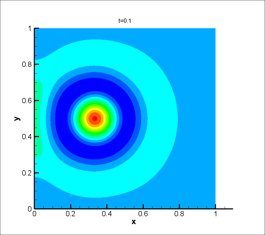
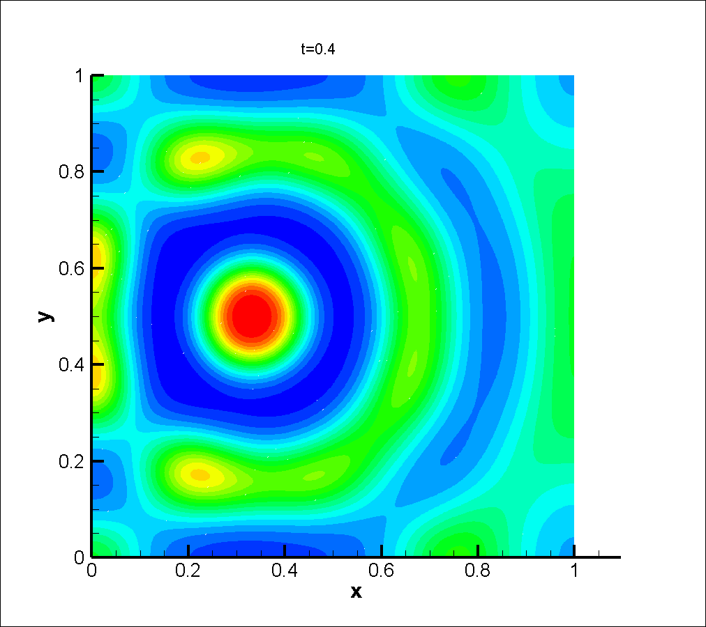
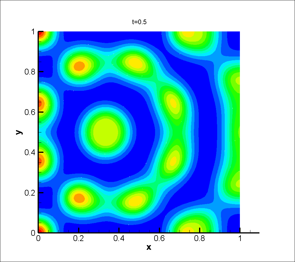
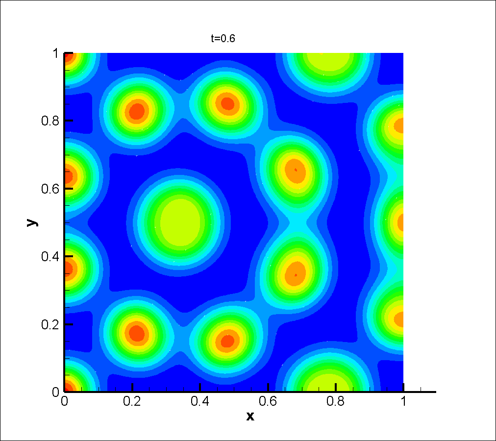
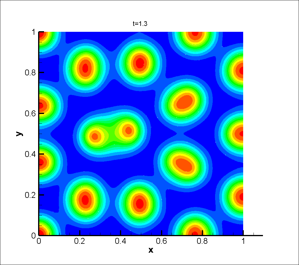
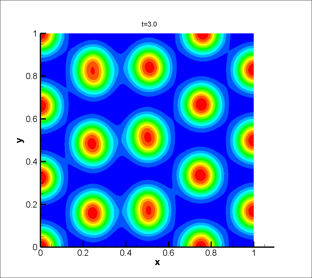
Figure 1: Contour plots of the time evolution of the concentration of the activator $C_{a}$ on the unit square.

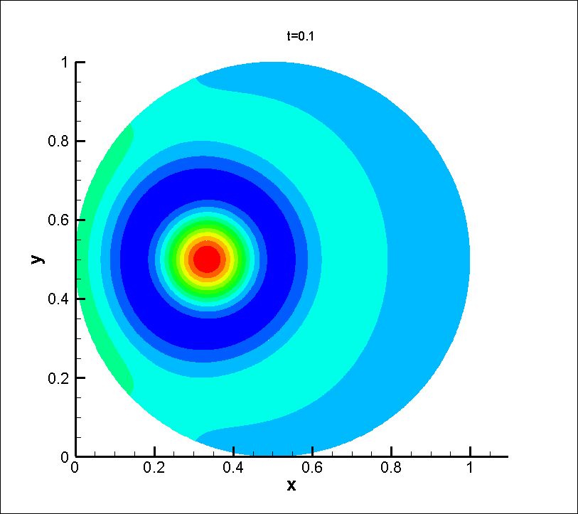
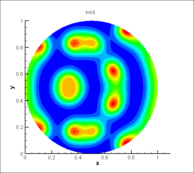
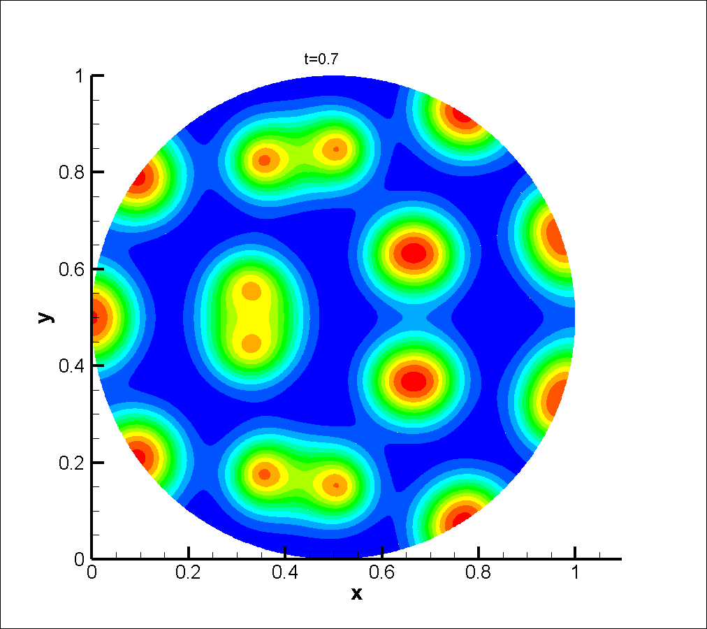
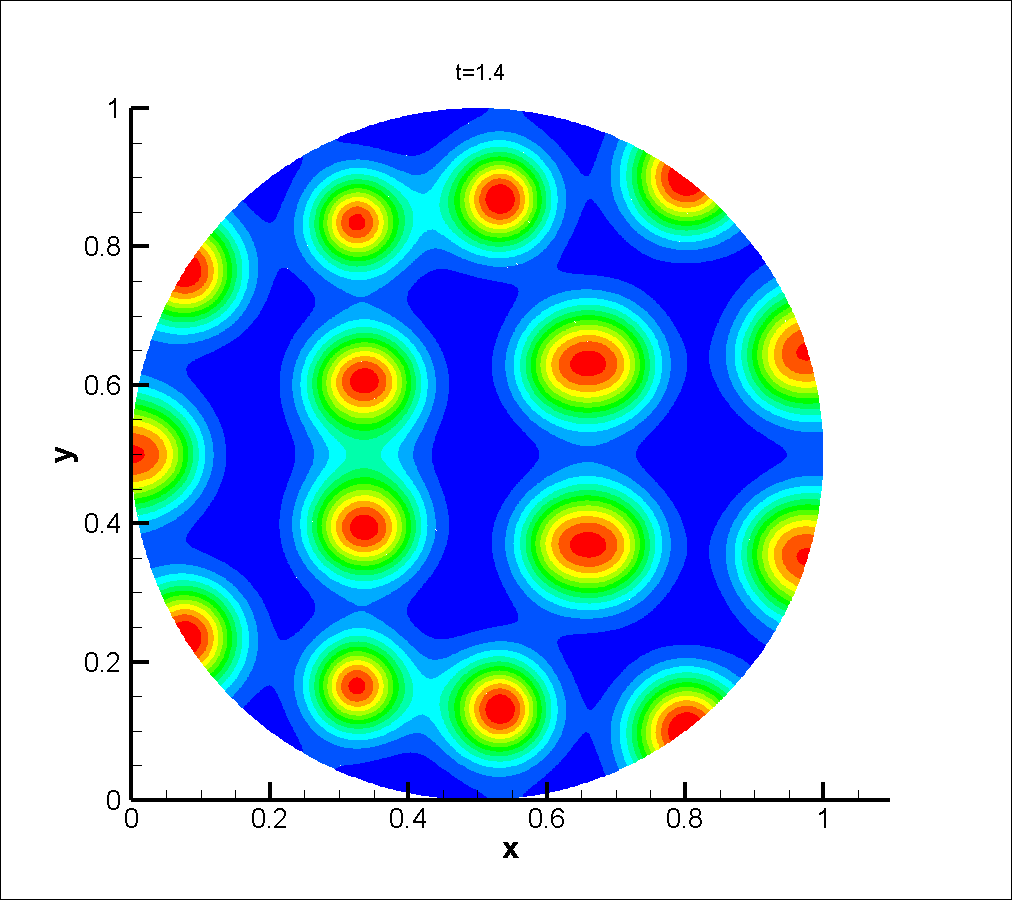
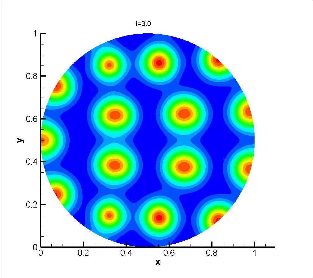
Figure 2: Contour plots of the time evolution of the concentration of the activator $C_{a}$ on the circular domain.

5 Conclusion

In our earlier work [8], we considered an Interpolatory HDG_k methods for semilinear parabolic PDEs with a general nonlinearity of the form $F(\nabla u,u)$. The interpolatory approach achieves optimal convergence rates and reduces the computational cost compared to standard HDG since all of the HDG matrices are assembled once before the time stepping procedure. However, the method does not have superconvergence by postprocessing.

In this work, we proposed a new superconvergent Interpolatory HDG_k method for approximating the solution of reaction diffusion PDEs. Unlike our earlier Interpolatory HDG_k work [8], the new method uses a postprocessing $u_{h}^{\star}$ to evaluate the nonlinear term. This change provides the superconvergence, and the new method also keeps all of the computational advantages of using an interpolatory approach for the nonlinear term. We proved the superconvergence under a global Lipschitz condition for the nonlinearity, and then extended the superconvergence results to a local Lipschitz condition assuming the mesh is quasi-uniform.

In the second part of this work [5], we again consider reaction diffusion equations and extend the ideas here to derive other superconvergent interpolatory HDG methods inspired by hybrid high-order methods [9]. However, it is currently not clear whether the present approach can be used to obtain the superconvergence for semilinear PDEs with a general nonlinearity $F(\nabla u,u)$. We are currently exploring this issue.

6 Appendix A

Recall the steady state problem (3.16) from Section 3.2.4, which we repeat here for convenience: let $(\overline{\bm{q}}_{h},\overline{u}_{h},\widehat{\overline{u}}_{h})\in\bm{V}_{h}\times W_{h}\times M_{h}$ be the solution of

$$\mathscr{B}(\overline{\bm{q}}_{h},\overline{u}_{h},\widehat{\overline{u}}_{h},\bm{r}_{h},v_{h},\widehat{v}_{h})=(f-\Pi_{W}u_{t}-F(u),v_{h})_{\mathcal{T}_{h}},$$ (6.1)

for all $(\bm{r}_{h},v_{h},\widehat{v}_{h})\in\bm{V}_{h}\times W_{h}\times M_{h}$. Since $\Pi_{W}$ commutes with the time derivative, taking the partial derivative of (6.1) with respect to $t$ shows $(\partial_{t}\overline{\bm{q}}_{h},\partial_{t}\overline{u}_{h},\partial_{t}\widehat{\overline{u}}_{h})\in\bm{V}_{h}\times W_{h}\times M_{h}$ is the solution of

$$\mathscr{B}(\partial_{t}\overline{\bm{q}}_{h},\partial_{t}\overline{u}_{h},\partial_{t}\widehat{\overline{u}}_{h},\bm{r}_{h},v_{h},\widehat{v}_{h}) =(f_{t}-\Pi_{W}u_{tt}-F^{\prime}(u)u_{t},v_{h})_{\mathcal{T}_{h}},$$ (6.2)

for all $(\bm{r}_{h},v_{h},\widehat{v}_{h})\in\bm{V}_{h}\times W_{h}\times M_{h}$.

The proof of the following lemma is very similar to a proof in [15], hence we omit it here.

Lemma 6.1.

For $\varepsilon_{h}^{\overline{\bm{q}}}=\bm{\Pi}_{V}\bm{q}-\overline{\bm{q}}_{h}$, $\varepsilon_{h}^{\overline{u}}=\Pi_{W}{u}-\overline{u}_{h}$, and $\varepsilon_{h}^{\widehat{\overline{u}}}=P_{M}u-\widehat{\overline{u}}_{h}$, we have

$$\mathscr{B}(\varepsilon_{h}^{\overline{\bm{q}}},\varepsilon_{h}^{\overline{u}},\varepsilon_{h}^{\widehat{\overline{u}}};\bm{r}_{h},w_{h},\widehat{v}_{h})=(\bm{\Pi}_{V}\bm{q}-\bm{q},\bm{r}_{h})_{\mathcal{T}_{h}}+(\Pi_{W}u_{t}-u_{t},v_{h})_{\mathcal{T}_{h}},$$ (6.3)

for all $(\bm{r}_{h},v_{h},\widehat{v}_{h})\in\bm{V}_{h}\times W_{h}\times M_{h}$.

The next step is the consideration of the dual problem (3.1), which we again repeat for convenience: Let

$$\begin{split}\bm{\Phi}+\nabla\Psi&=0\qquad\qquad\text{in}\ \Omega,\\ \nabla\cdot\bm{\Phi}&=\Theta\qquad\quad~{}~{}\text{in}\ \Omega,\\ \Psi&=0\qquad\qquad\text{on}\ \partial\Omega.\end{split}$$ (6.4)

By the assumption at the beginning of Section 3, this boundary value problem admits the regularity estimate

$$\|\bm{\Phi}\|_{H^{1}(\Omega)}+\|\Psi\|_{H^{2}(\Omega)}\leq C\|\Theta\|_{L^{2}(\Omega)},$$ (6.5)

for all $\Theta\in L^{2}(\Omega)$.

Lemma 6.2.

We have

$$\|\varepsilon^{\overline{u}}_{h}\|_{\mathcal{T}_{h}} \leq Ch^{\min\{k,1\}}(\|\bm{q}-\bm{\Pi}_{V}\bm{q}\|_{\mathcal{T}_{h}}+\|u_{t}-\Pi_{W}u_{t}\|_{\mathcal{T}_{h}})$$

$$\|\varepsilon^{\overline{\bm{q}}}_{h}\|_{\mathcal{T}_{h}} \leq C(\|\bm{q}-\bm{\Pi}_{V}\bm{q}\|_{\mathcal{T}_{h}}+\|u_{t}-\Pi_{W}u_{t}\|_{\mathcal{T}_{h}}).$$

Proof.

Let $\Theta=\varepsilon_{h}^{\overline{u}}$ in the dual problem (6.4), and take $(\bm{r}_{h},v_{h},\widehat{v}_{h})=(-\bm{\Pi}_{V}\bm{\Phi},\Pi_{W}\Psi,P_{M}\Psi)$ in the definition of $\mathscr{B}$ (3.8) to get

$$\mathscr{B} (\varepsilon^{\overline{\bm{q}}}_{h},\varepsilon^{\overline{u}}_{h},\varepsilon^{\widehat{\overline{u}}}_{h};-\bm{\Pi}_{V}\bm{\Phi},\Pi_{W}\Psi,P_{M}\Psi)$$

$$=-(\varepsilon^{\overline{\bm{q}}}_{h},\bm{\Pi}_{V}\bm{\Phi})_{\mathcal{T}_{h}}+(\varepsilon^{\overline{u}}_{h},\nabla\cdot\bm{\Pi}_{V}\bm{\Phi})_{\mathcal{T}_{h}}-\langle\varepsilon^{\widehat{\overline{u}}}_{h},\bm{\Pi}_{V}\bm{\Phi}\cdot\bm{n}\rangle_{\partial\mathcal{T}_{h}}+(\nabla\cdot\varepsilon^{\overline{\bm{q}}}_{h},\Pi_{W}\Psi)_{\mathcal{T}_{h}}$$

$$\quad-\langle\varepsilon^{\overline{\bm{q}}}_{h}\cdot\bm{n},P_{M}\Psi\rangle_{\partial{\mathcal{T}_{h}}}+\left\langle\tau(\varepsilon^{\overline{u}}_{h}-\varepsilon^{\widehat{\overline{u}}}_{h}),\Pi_{W}\Psi-P_{M}\Psi\right\rangle_{\partial\mathcal{T}_{h}}$$

$$=-(\varepsilon^{\overline{\bm{q}}}_{h},\bm{\Phi})_{\mathcal{T}_{h}}+(\varepsilon^{\overline{\bm{q}}}_{h},\bm{\Phi}-\bm{\Pi}_{V}\bm{\Phi})_{\mathcal{T}_{h}}+(\varepsilon^{\overline{u}}_{h},\nabla\cdot\bm{\Phi})_{\mathcal{T}_{h}}-(\varepsilon^{\overline{u}}_{h},\nabla\cdot(\bm{\Phi}-\bm{\Pi}_{V}\bm{\Phi}))_{\mathcal{T}_{h}}$$

$$\quad+\langle\varepsilon^{\widehat{\overline{u}}}_{h},(\bm{\Phi}-\bm{\Pi}_{V}\bm{\Phi})\cdot\bm{n}\rangle_{\partial\mathcal{T}_{h}}+(\nabla\cdot\varepsilon^{\overline{\bm{q}}}_{h},\Psi)_{\mathcal{T}_{h}}+(\nabla\cdot\varepsilon^{\overline{\bm{q}}}_{h},\Pi_{W}\Psi-\Psi)_{\mathcal{T}_{h}}$$

$$\quad-\langle\varepsilon^{\overline{\bm{q}}}_{h}\cdot\bm{n},\Psi\rangle_{\partial{\mathcal{T}_{h}}}+\left\langle\tau(\varepsilon^{\overline{u}}_{h}-\varepsilon^{\widehat{\overline{u}}}_{h}),\Pi_{W}\Psi-P_{M}\Psi\right\rangle_{\partial\mathcal{T}_{h}}$$

$$=(\varepsilon^{\overline{\bm{q}}}_{h},\bm{\Phi}-\bm{\Pi}_{V}\bm{\Phi})_{\mathcal{T}_{h}}+\|\varepsilon^{\overline{u}}_{h}\|_{\mathcal{T}_{h}}^{2}.$$

On the other hand, take $(\bm{r}_{h},v_{h},\widehat{v}_{h})=(-\bm{\Pi}_{V}\bm{\Phi},\Pi_{W}\Psi,P_{M}\Psi)$ in (6.3) to get

$$\mathscr{B}(\varepsilon^{\overline{\bm{q}}}_{h},\varepsilon^{\overline{u}}_{h},\varepsilon^{\widehat{\overline{u}}}_{h};-\bm{\Pi}_{V}\bm{\Phi},\Pi_{W}\Psi,P_{M}\Psi)=(\bm{q}-\bm{\Pi}_{V}\bm{q},\bm{\Pi}_{V}\bm{\Phi})_{\mathcal{T}_{h}}+(\Pi_{W}u_{t}-u_{t},\Pi_{W}\Psi)_{\mathcal{T}_{h}}.$$ (6.6)

Comparing the above two equalities gives

$$\|\varepsilon^{\overline{u}}_{h}\|^{2}_{\mathcal{T}_{h}} =-(\varepsilon^{\overline{\bm{q}}}_{h},\bm{\Phi}-\bm{\Pi}_{V}\bm{\Phi})_{\mathcal{T}_{h}}+(\bm{q}-\bm{\Pi}_{V}\bm{q},\bm{\Pi}_{V}\bm{\Phi})_{\mathcal{T}_{h}}+(\Pi_{W}u_{t}-u_{t},\Pi_{W}\Psi)_{\mathcal{T}_{h}}$$

$$=-(\varepsilon^{\overline{\bm{q}}}_{h},\bm{\Phi}-\bm{\Pi}_{V}\bm{\Phi})_{\mathcal{T}_{h}}+(\bm{q}-\bm{\Pi}_{V}\bm{q},\bm{\Pi}_{V}\bm{\Phi}-\bm{\Phi})_{\mathcal{T}_{h}}$$

$$\quad+(\bm{q}-\bm{\Pi}_{V}\bm{q},\bm{\Phi})_{\mathcal{T}_{h}}+(\Pi_{W}u_{t}-u_{t},\Pi_{W}\Psi)_{\mathcal{T}_{h}}$$

$$=-(\varepsilon^{\overline{\bm{q}}}_{h},\bm{\Phi}-\bm{\Pi}_{V}\bm{\Phi})_{\mathcal{T}_{h}}+(\bm{q}-\bm{\Pi}_{V}\bm{q},\bm{\Pi}_{V}\bm{\Phi}-\bm{\Phi})_{\mathcal{T}_{h}}$$

$$\quad-(\bm{q}-\bm{\Pi}_{V}\bm{q},\nabla\Psi)_{\mathcal{T}_{h}}+(\Pi_{W}u_{t}-u_{t},\Pi_{W}\Psi)_{\mathcal{T}_{h}}$$

$$=-(\varepsilon^{\overline{\bm{q}}}_{h},\bm{\Phi}-\bm{\Pi}_{V}\bm{\Phi})_{\mathcal{T}_{h}}+(\bm{q}-\bm{\Pi}_{V}\bm{q},\bm{\Pi}_{V}\bm{\Phi}-\bm{\Phi})_{\mathcal{T}_{h}}$$

$$\quad-(\bm{q}-\bm{\Pi}_{V}\bm{q},\nabla(\Psi-\Pi_{W}\Psi))_{\mathcal{T}_{h}}+(\Pi_{W}u_{t}-u_{t},\Pi_{W}\Psi-\min\{k,1\}\Pi_{0}\Psi)_{\mathcal{T}_{h}}.$$

Hence, by the regularity of the dual PDE (6.5), we have

$$\|\varepsilon^{\overline{u}}_{h}\|^{2}_{\mathcal{T}_{h}}\leq Ch^{2}\|\varepsilon^{\overline{\bm{q}}}_{h}\|_{\mathcal{T}_{h}}^{2}+Ch^{\min\{2k,2\}}\|\bm{q}-\bm{\Pi}_{V}\bm{q}\|_{\mathcal{T}_{h}}^{2}+Ch^{\min\{2k,2\}}\|u_{t}-\Pi_{W}u_{t}\|_{\mathcal{T}_{h}}^{2}.$$ (6.7)

Next, take $(\bm{r}_{h},v_{h},\widehat{v}_{h})=(\varepsilon_{h}^{\overline{\bm{q}}},\varepsilon_{h}^{\overline{u}},\varepsilon_{h}^{\widehat{\overline{u}}})$ in (6.3) to obtain

$$\|\varepsilon_{h}^{\overline{\bm{q}}}\|^{2}_{\mathcal{T}_{h}}+\langle\tau(\varepsilon_{h}^{\overline{u}}-\varepsilon_{h}^{\widehat{\overline{u}}}),\varepsilon_{h}^{\overline{u}}-\varepsilon_{h}^{\widehat{\overline{u}}}\rangle_{\partial{\mathcal{T}_{h}}}$$

$$=(\bm{\Pi}_{V}{\bm{q}}-\bm{q},\varepsilon_{h}^{\overline{\bm{q}}})_{\mathcal{T}_{h}}+(\Pi_{W}u_{t}-u_{t},\varepsilon_{h}^{\overline{u}})_{\mathcal{T}_{h}}$$

$$\leq C\|\bm{\Pi}_{V}{\bm{q}}-\bm{q}\|_{\mathcal{T}_{h}}^{2}+\frac{1}{2}\|\varepsilon_{h}^{\overline{\bm{q}}}\|^{2}_{\mathcal{T}_{h}}+4C\|\Pi_{W}u_{t}-u_{t}\|_{\mathcal{T}_{h}}^{2}+\frac{1}{4C}\|\varepsilon_{h}^{\overline{u}}\|_{\mathcal{T}_{h}}^{2}.$$

This implies

$$\|\varepsilon_{h}^{\overline{\bm{q}}}\|^{2}_{\mathcal{T}_{h}}+\langle\tau(\varepsilon_{h}^{\overline{u}}-\varepsilon_{h}^{\widehat{\overline{u}}}),\varepsilon_{h}^{\overline{u}}-\varepsilon_{h}^{\widehat{\overline{u}}}\rangle_{\partial{\mathcal{T}_{h}}}\leq 2C\|\bm{\Pi}_{V}{\bm{q}}-\bm{q}\|_{\mathcal{T}_{h}}^{2}+8C\|\Pi_{W}u_{t}-u_{t}\|_{\mathcal{T}_{h}}^{2}+\frac{1}{2C}\|\varepsilon_{h}^{\overline{u}}\|_{\mathcal{T}_{h}}^{2}.$$ (6.8)

Next, use $h\leq 1$ and substitute (6.8) into (6.7) to yield the result. ∎

Following the same steps, we obtain the following result:

Lemma 6.3.

We have

$$\|\partial_{t}(\Pi_{W}u-\overline{u}_{h})\|_{\mathcal{T}_{h}} \leq Ch^{\min\{k,1\}}(\|\bm{q}_{t}-\bm{\Pi}_{V}\bm{q}_{t}\|_{\mathcal{T}_{h}}+\|u_{tt}-\Pi_{W}u_{tt}\|_{\mathcal{T}_{h}}).$$

References

- [1] Susanne C. Brenner and L. Ridgway Scott. The mathematical theory of finite element methods, volume 15 of Texts in Applied Mathematics. Springer, New York, third edition, 2008.
- [2] Aycil Cesmelioglu, Bernardo Cockburn, and Weifeng Qiu. Analysis of a hybridizable discontinuous Galerkin method for the steady-state incompressible Navier-Stokes equations. Math. Comp., 86(306):1643–1670, 2017.
- [3] Brandon Chabaud and Bernardo Cockburn. Uniform-in-time superconvergence of HDG methods for the heat equation. Math. Comp., 81(277):107–129, 2012.
- [4] Chuan Miao Chen, Stig Larsson, and Nai Ying Zhang. Error estimates of optimal order for finite element methods with interpolated coefficients for the nonlinear heat equation. IMA J. Numer. Anal., 9(4):507–524, 1989.
- [5] G. Chen, B. Cockburn, J. R. Singler, and Y. Zhang. Superconvergent Group HDG methods for reaction diffusion equations II: HHO-inspired methods. In preparation.
- [6] Zhangxin Chen and Jim Douglas, Jr. Approximation of coefficients in hybrid and mixed methods for nonlinear parabolic problems. Mat. Apl. Comput., 10(2):137–160, 1991.
- [7] I. Christie, D. F. Griffiths, A. R. Mitchell, and J. M. Sanz-Serna. Product approximation for nonlinear problems in the finite element method. IMA J. Numer. Anal., 1(3):253–266, 1981.
- [8] B. Cockburn, J. R. Singler, and Y. Zhang. Interpolatory HDG Methods for Parabolic Semilinear PDEs. J. Sci. Comput. In revision.
- [9] Bernardo Cockburn, Daniele A. Di Pietro, and Alexandre Ern. Bridging the hybrid high-order and hybridizable discontinuous Galerkin methods. ESAIM Math. Model. Numer. Anal., 50(3):635–650, 2016.
- [10] Bernardo Cockburn and Guosheng Fu. Superconvergence by -decompositions. Part II: Construction of two-dimensional finite elements. ESAIM Math. Model. Numer. Anal., 51(1):165–186, 2017.
- [11] Bernardo Cockburn and Guosheng Fu. Superconvergence by -decompositions. Part III: Construction of three-dimensional finite elements. ESAIM Math. Model. Numer. Anal., 51(1):365–398, 2017.
- [12] Bernardo Cockburn, Guosheng Fu, and Francisco-Javier. Sayas. Superconvergence by -decompositions. Part I: General theory for HDG methods for diffusion. Math. Comp., 86(306):1609–1641, 2017.
- [13] Bernardo Cockburn, Jayadeep Gopalakrishnan, and Raytcho Lazarov. Unified hybridization of discontinuous Galerkin, mixed, and continuous Galerkin methods for second order elliptic problems. SIAM J. Numer. Anal., 47(2):1319–1365, 2009.
- [14] Bernardo Cockburn, Jayadeep Gopalakrishnan, Ngoc Cuong Nguyen, Jaume Peraire, and Francisco-Javier Sayas. Analysis of HDG methods for Stokes flow. Math. Comp., 80(274):723–760, 2011.
- [15] Bernardo Cockburn, Jayadeep Gopalakrishnan, and Francisco-Javier Sayas. A projection-based error analysis of HDG methods. Math. Comp., 79(271):1351–1367, 2010.
- [16] Bernardo Cockburn and Jiguang Shen. A hybridizable discontinuous Galerkin method for the -Laplacian. SIAM J. Sci. Comput., 38(1):A545–A566, 2016.
- [17] Benjamin T. Dickinson and John R. Singler. Nonlinear model reduction using group proper orthogonal decomposition. Int. J. Numer. Anal. Model., 7(2):356–372, 2010.
- [18] Jim Douglas, Jr. and Todd Dupont. The effect of interpolating the coefficients in nonlinear parabolic Galerkin procedures. Math. Comput., 20(130):360–389, 1975.
- [19] C. A. J. Fletcher. The group finite element formulation. Comput. Methods Appl. Mech. Engrg., 37(2):225–244, 1983.
- [20] C. A. J. Fletcher. Time-splitting and the group finite element formulation. In Computational techniques and applications: CTAC-83 (Sydney, 1983), pages 517–532. North-Holland, Amsterdam, 1984.
- [21] Hardik Kabaria, Adrian J. Lew, and B. Cockburn. A hybridizable discontinuous Galerkin formulation for non-linear elasticity. Comput. Methods Appl. Mech. Engrg., 283:303–329, 2015.
- [22] Dongho Kim, Eun-Jae Park, and Boyoon Seo. Two-scale product approximation for semilinear parabolic problems in mixed methods. J. Korean Math. Soc., 51(2):267–288, 2014.
- [23] Stig Larsson, Vidar Thomée, and Nai Ying Zhang. Interpolation of coefficients and transformation of the dependent variable in finite element methods for the nonlinear heat equation. Math. Methods Appl. Sci., 11(1):105–124, 1989.
- [24] J. C. López Marcos and J. M. Sanz-Serna. Stability and convergence in numerical analysis. III. Linear investigation of nonlinear stability. IMA J. Numer. Anal., 8(1):71–84, 1988.
- [25] D. Moro, N.-C. Nguyen, and J. Peraire. A hybridized discontinuous Petrov-Galerkin scheme for scalar conservation laws. Internat. J. Numer. Methods Engrg., 91:950–970, 2012.
- [26] N. C. Nguyen and J. Peraire. Hybridizable discontinuous Galerkin methods for partial differential equations in continuum mechanics. J. Comput. Phys., 231:5955–5988, 2012.
- [27] N. C. Nguyen, J. Peraire, and B. Cockburn. An implicit high-order hybridizable discontinuous Galerkin method for linear convection-diffusion equations. J. Comput. Phys., 228(9):3232–3254, 2009.
- [28] N. C. Nguyen, J. Peraire, and B. Cockburn. An implicit high-order hybridizable discontinuous Galerkin method for nonlinear convection-diffusion equations. J. Comput. Phys., 228(23):8841–8855, 2009.
- [29] N. C. Nguyen, J. Peraire, and B. Cockburn. A hybridizable discontinuous Galerkin method for the incompressible Navier-Stokes equations (AIAA Paper 2010-362). In Proceedings of the 48th AIAA Aerospace Sciences Meeting and Exhibit, Orlando, Florida, January 2010.
- [30] N. C. Nguyen, J. Peraire, and B. Cockburn. A class of embedded discontinuous Galerkin methods for computational fluid dynamics. J. Comput. Phys., 302:674–692, 2015.
- [31] J. Peraire, N. C. Nguyen, and B. Cockburn. A hybridizable discontinuous Galerkin method for the compressible Euler and Navier-Stokes equations (AIAA Paper 2010-363). In Proceedings of the 48th AIAA Aerospace Sciences Meeting and Exhibit, Orlando, Florida, January 2010.
- [32] J. M. Sanz-Serna and L. Abia. Interpolation of the coefficients in nonlinear elliptic Galerkin procedures. SIAM J. Numer. Anal., 21(1):77–83, 1984.
- [33] Rolf Stenberg. Postprocessing schemes for some mixed finite elements. RAIRO Modél. Math. Anal. Numér., 25(1):151–167, 1991.
- [34] Yves Tourigny. Product approximation for nonlinear Klein-Gordon equations. IMA J. Numer. Anal., 10(3):449–462, 1990.
- [35] Cheng Wang. Convergence of the interpolated coefficient finite element method for the two-dimensional elliptic sine-Gordon equations. Numer. Methods Partial Differential Equations, 27(2):387–398, 2011.
- [36] Zhu Wang. Nonlinear model reduction based on the finite element method with interpolated coefficients: semilinear parabolic equations. Numer. Methods Partial Differential Equations, 31(6):1713–1741, 2015.
- [37] Mary Fanett Wheeler. A priori error estimates for Galerkin approximations to parabolic partial differential equations. SIAM J. Numer. Anal., 10:723–759, 1973.
- [38] Ziqing Xie and Chuanmiao Chen. The interpolated coefficient FEM and its application in computing the multiple solutions of semilinear elliptic problems. Int. J. Numer. Anal. Model., 2(1):97–106, 2005.
- [39] Zhiguang Xiong and Chuanmiao Chen. Superconvergence of rectangular finite element with interpolated coefficients for semilinear elliptic problem. Appl. Math. Comput., 181(2):1577–1584, 2006.
- [40] Zhiguang Xiong and Chuanmiao Chen. Superconvergence of triangular quadratic finite element with interpolated coefficients for semilinear parabolic equation. Appl. Math. Comput., 184(2):901–907, 2007.
- [41] Zhiguang Xiong, Yanping Chen, and Yan Zhang. Convergence of FEM with interpolated coefficients for semilinear hyperbolic equation. J. Comput. Appl. Math., 214(1):313–317, 2008.
- [42] Jianfeng Zhu, Yong-Tao Zhang, Stuart A. Newman, and Mark Alber. Application of discontinuous Galerkin methods for reaction-diffusion systems in developmental biology. J. Sci. Comput., 40(1-3):391–418, 2009.