The compact multiple system HIP 41431

Abstract

The nearby (50 pc) K7V dwarf HIP 41431 (EPIC 212096658) is a compact 3-tier hierarchy. Three K7V stars with similar masses, from 0.61 to 0.63 solar, make a triple-lined spectroscopic system where the inner binary with a period of 2.9 days is eclipsing, and the outer companion on a 59-day orbit exerts strong dynamical influence revealed by the eclipse time variation in the Kepler photometry. Moreover, the centre-of-mass of the triple system moves on a 3.9-year orbit, modulating the proper motion. The mass of the 4-th star is 0.35 solar. The Kepler and ground-based photometry and radial velocities from four different spectrographs are used to adjust the spectro-photodynamical model that accounts for dynamical interaction. The mutual inclination between the two inner orbits is 2$\aas@@fstack{\circ}$16$\pm$0$\aas@@fstack{\circ}$11, while the outer orbit is inclined to their common plane by 21°$\pm$16°. The inner orbit precesses under the influence of both outer orbits, causing observable variation of the eclipse depth. Moreover, the phase of the inner binary is strongly modulated with a 59-day period and its line of apsides precesses. The middle orbit with eccentricity $e=0.28$ also precesses, causing the observed variation of its radial velocity curve. Masses and other parameters of stars in this unique hierarchy are determined. This system is dynamically stable and likely old.

1 Introduction

Study of stellar hierachies containing three or more bodies helps to understand their origin, still a matter of controversy and debate. Although the main aspects of star formation are well understood, the genesis of stellar systems, particularly close binaries, is obscure because the mechanisms reponsible for bringing together two or more stars, initially formed at a much larger separation, are not identified or modelled. From the observational side, establishing a reliable statistics of hierarchies is a basis for testing theoretical predictions. However, individual systems with rare and/or extreme characteristics are equally enlightening, as such objects challenge the formation theories and extend the boundaries of the explored parameter space. This is the case under study here.

We investigate an interesting low-mass hierarchical stellar system, HIP 41431 (GJ 307). Basic data on this star collected with the help of Simbad are assembled in Table 1. This object came to the attention of the present authors independently as a triple-lined spectroscopic system (D.L. and J.S.) and as an eclipsing binary, exhibiting fast and large amplitude eclipse timing variations (ETV) of likely dynamical origin (T.B. and T.H.). Its architecture is illustrated in Fig. 1, where the three spectroscopically visible components with comparable masses and luminosities are designated as A, B, and C. The fourth star D was discovered by the modulation of radial velocity (RV) of the centre of mass of the inner triple and from the residuals of the dynamical, three-body ETV model, and confirmed by its astrometric signature in the Gaia catalog. All orbits seem to be close to one plane and have small eccentricities, resembling in this sense a solar system, like the “planetary” quadruple star HD 91962 (Tokovinin et al., 2015). In these systems, the moderate period ratios on the order of 20 favor dynamical interaction between inner and outer orbits, so the motion cannot be modelled as a superposition of independent Keplerian orbits. However, compared to HD 91962, HIP 41431 is much more compact and fast.

The paper begins with a short description of the data in Section 2. Then in Section 3 we present and discuss spectroscopic orbits and determine the preliminary components’ masses. Global dynamical modelling of the Kepler K2 and ground-based photometry and the RVs is presented in Section 4. Its results are confronted with empirical and theoretical stellar properties in § 5. Observed effects associated with dynamical interaction between the orbits are covered in Section 6. We summarize and discuss our findings in Section 7.

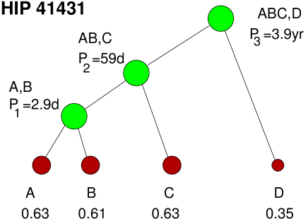
Figure 1: Architecture of the quadruple system HIP 41431. Brown circles denote stars A to D, the numbers are their masses, green circles are subsystems.

2 Observational data

Table 1: Main characteristics of HIP 41431

Parameter	Value
Identifiers	HIP 41431, GJ 307
	EPIC 212096658
Position (J2000, Gaia DR2)	08:27:00.91, +21:57:24.7
PM $\mu_{\alpha}$, $\mu_{\delta}$ (mas yr-1, UCAC4)	+9.2$\pm$1.1, +21.08$\pm$1.1
Parallax (mas, Gaia DR2)	20.06 $\pm$ 0.09
Spectral type	K7V
Optical photometry $B$, $V$, $G$ (mag)	13.01, 10.84, 10.15
Infrared photometry $J$, $H$, $K$ (mag)	8.02, 7.37, 7.19
Spatial velocity $U,V,W$ (km s-1 )	8.1, 7.7, $-$1.4

2.1 Photometric observations

2.1.1 Kepler K2 photometry

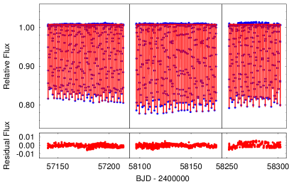
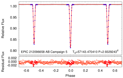
Figure 2: The K2 lightcurves of HIP 41431 (EPIC 212096658). Left panel: The Campaigns 5, 16 and 18 long cadence PDCSAP lightcurves (blue circles) indicate moderate eclipse depth variations from campaign to campaign (see text for details). Red lines show our spectro-photodynamical model solution (Sect. 4). Right panel: The phase-folded, binned, and averaged Campaign 5 K2-lightcurve of the innermost binary. The phased averages of the observed flux near the eclipses are plotted by the blue circles (these data were used for the joint spectro-photodynamical analysis), while the out-of-eclipse flux is plotted by grey circles. The red curve is the folded, binned and averaged lightcurve of the cadence-time corrected photodynamical model solution calculated at the time of each observation; the residuals to the model are also shown in the bottom panels.

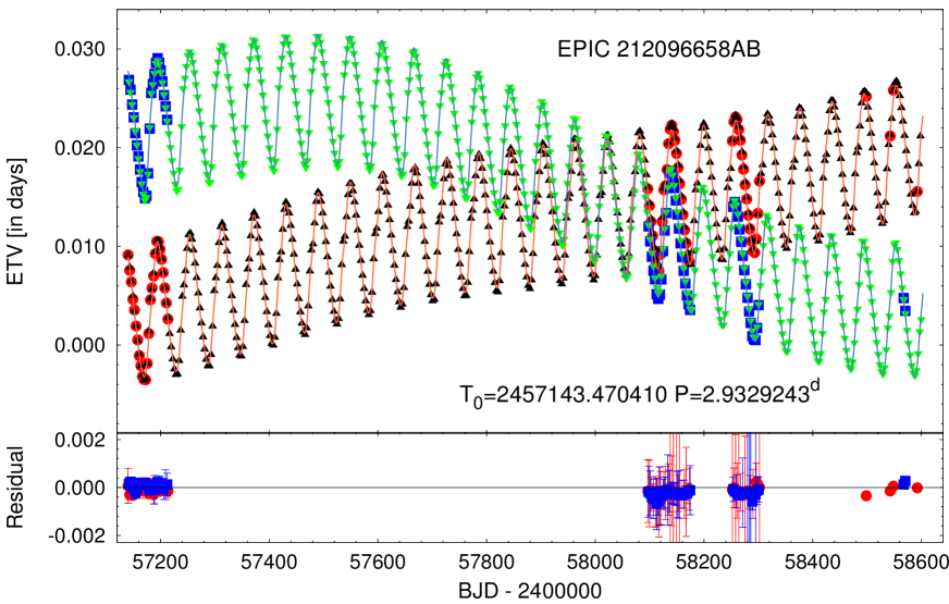
Figure 3: Eclipse timing variations of the innermost, eclipsing pair. Red circles and blue boxes stand for the primary and secondary ETVs, respectively, calculated from the observed eclipse events, while black upward and green downward triangles show the corresponding primary and secondary ETV, determined from the spectro-photodynamical model solution. Furthermore, orange and lightblue lines represent approximate analytical ETV models for the primary and secondary eclipses. The residuals of the observed vs photodynamically modelled ETVs are plotted in the bottom panel.

HIP 41431 was observed with Kepler spacecraft (Borucki et al., 2010) in long cadence (LC) mode during Campaigns 5, 16 and 18 of K2 mission. Furthermore, in Campaign 18 short cadence (SC) data were also collected. Eclipses with a period of 2.93291 days in the C5 data were reported by Barros et al. (2016). Figure 2 shows the K2 photometry and its model discussed below.

We determined the mid-time of each observed eclipse and generated the ETV curves. The method we used is described in detail by Borkovits et al. (2016). The times of minima are listed in Table 5, while the ETV curves are shown in Fig. 3. The amplitude of the cyclic variation with the 60-d period is 0.007 d, an order of magnitude larger than the light-time delay in the outer orbit. This variation is caused primarily by the interaction with the star C that modulates the orbital elements of the inner orbit, including its period. Moreover, the inner orbit has a fast apsidal rotation which is also forced dynamically by star C.

In such a compact, strongly interacting triple system, even marginally (by $\approx 1-2\degr$) misaligned inner and outer orbital planes produce fast precession of the inner orbit and, hence, eclipse depth variations. Therefore, we checked the K2 lightcurves for such features. Raw K2 LC data are processed and corrected with different pipelines, resulting in somewhat different lightcurves. We downloaded from the Barbara A. Mikulski Archive for Space Telescopes (MAST) and investigated the PDCSAP lightcurves obtained with the Kepler/K2 pipeline and the K2 self-flat-fielding (K2SFF) pipeline of Vanderburg & Johnson (2014). Regarding the PDCSAP lightcurves, normalizing the flux levels of each of the three datasets to their out-of-eclipse averages reveals that the eclipses in the C16 and C18 data are deeper by about $\approx 6$% and $1.5$%, respectively, relative to the C5 data. The same feature can be identified in the K2SFF lightcurves, too. This finding, however, does not mean automatically that the eclipse depth variation is real. Different locations of the target on the Kepler’s CCDs and different aperture masks used for the photometry in these datasets may produce apparent eclipse depth variation because of different amounts of contaminating fluxes from other stars within the apertures. However, there are no stars brighter than $G=19.7$ mag within $1.2^{\prime}$ radius from our target in the Gaia DR2 catalog. We conclude that slight eclipse depth variation during the observing window of K2 photometry is possible, although it cannot be proven conclusively. Therefore, we decided to apply our photodynamical modelling package both for the uneven and the uniform eclipse depth lightcurve. For the latter, we transformed the C5 and C18 lightcurves to have equal eclipse depths to the C16 data which exhibit the deepest eclipses.

2.1.2 Ground-based follow up photometry

In order to monitor the possible quick eclipse depth variations and to lengthen the interval of the available ETV data suitable for the study of the dynamical evolution of the system, we carried out additional eclipse event observations with the 0.5 m telescope of Baja Astronomical Observatory of Szeged University located at Baja, Hungary, and equipped with an SBIG ST-6303 CCD detector. The target was observed on 7 nights between Jan 14 and Apr 18, 2019, which led to the determination of 6 additional times of minima data (see also in Fig. 3 and Table 5). The usual data reduction and photometric analysis were performed using IRAF routines.

As shown below in Sect. 6, these observations confirmed not only the existence, but even the rate of the eclipse depth variations that was predicted by the uneven eclipse depth model solution.

2.2 High-resolution spectroscopy

High-resolution spectroscopy was conducted independently using several facilities. The primary goal was measurement of RVs for orbit determination. Stellar parameters such as rotation, metallicity and gravity can be determined as well from the spectra. We tabulate the measured radial velocities in Table 6.

2.2.1 CfA observations

This nearby star was observed with two identical CfA Digital Speedometers (Latham, 1985, 1992) from 1999.3 till 2008.3. Seven observations were carried out with the instrument installed at the 1.5-m Wyeth Reflector at the Oak Ridge Observatory in the town of Harvard, Massachusetts. The other spectra were obtained with the 1.5-m Tillinghast Reflector at the Whipple Observatory on Mount Hopkins, Arizona. A total of 102 observations were collected. The RVs were measured by correlations of the single echelle order centered on the Mg b triplet near 519 nm, with a wavelength window of 4.5 nm and resolving power of 35 000. As the spectrum is triple-lined, the TRICOR algorithm was used, analogous to TODCOR (Zucker & Mazeh, 1994). A correction of +0.14 km s^-1 must be added to these RVs to put them on the IAU system. D.L. found the flux ratio C:A:B of 1:0.94:0.78 at 5187Å.

In 2009, the new fibre-fed Tillinghast Reflector Echelle Spectrograph (TRES; Szentgyorgyi & Furész, 2007) was used to obtain an additional spectrum, followed by five more spectra taken in 2014. We measured the RVs by cross-correlating these spectra with the binary mask and applied the zero-point correction of $-0.62$ km s^-1 appropriate for this instrument.

2.2.2 VUES observations

Figure 4: CCFs of HIP 41431 recorded with VUES, with vertical shifts. The reduced Julian dates are indicated on the right.

One of the authors (J.S.) has been conducting a long-term RV survey of nearby low-mass stars using several spectrometers. Most data are obtained at the 1.65-m telescope at the Moletai observatory in Lithuania (Sperauskas et al., 2016). A CORAVEL-type spectrometer was used to measure the RVs with a typical accuracy of the order of km s^-1 and a spectral resolution around 20000. HIP 43431 was observed with CORAVEL at Moletai several times in the period from 2000 to 2014. Owing to the relative faintess of the star and the complex multi-line nature of its spectrum, the CCF dips are noisy and often blended. In this paper, we do not use these CORAVEL observations.

In 2015, a modern fibre-fed echelle spectrometer VUES (Jurgenson et al., 2016) was commissioned at Moletai. We took spectra of HIP 43431 with a resolution of 30 000 in the wavelength range from 400 to 880 nm. The spectra recorded by the CCD detector are extracted and calibrated in the standard way. The RV is determined by numerical cross-correlation of the spectrum with a binary mask, emulating the CORAVEL method in software (Fig. 4). Compared to CORAVEL, the RVs delivered by VUES are more accurate; their rms residuals from the orbits are, typically, from 0.2 to 0.3 km s^-1 . For each observing night, the instrumental velocity zero point and its drift were checked by observations of a few RV standard stars. The mean RV zero-point, calculated using 186 measurements of the standard stars, is $\Delta$RV=0.09$\pm$0.01 km s^-1 , and the standard deviation is 0.19 km s^-1 . One can suspect a small drift of the zero-point from 0.04 to 0.14 km s^-1 in about three years. Practically the same value of $\Delta$RV=0.08$\pm$0.05 km s^-1 (rms 0.18 km s^-1 , $n=15$) is obtained using telluric lines in the spectra of HIP 41431 as the RV reference.

2.2.3 CHIRON observations

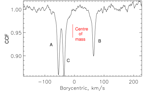
Figure 5: CCF of HIP 41431 using the CHIRON spectrum taken on JD 2458443.8.

Seven spectra of HIP 41431 were taken at the 1.5-m telescope located at Cerro Tololo (Chile) and operated by the SMARTS consortium. Observations were conducted by the telescope operator in the service mode. The optical echelle spectrometer CHIRON (Tokovinin et al., 2013) was used in the slicer mode with a spectral resolution of 80000. On each visit, a single 10-minute exposure of the star was taken, accompanied by the spectrum of the comparison lamp for wavelength calibration. The data were reduced by the pipeline written in IDL.

The RVs are derived from the reduced spectra by cross-correlation with a binary mask based on the solar spectrum, similarly to the CORAVEL RVs. More details are provided by Tokovinin (2016). Only the spectral range from 4500Å to 6500Å, relatively free from telluric lines, was used for the CCF calculation. The RVs delivered by this procedure should be on the absolute scale if the wavelength calibration is good. A comparison of CHIRON RVs with several RV standards revealed a small offset of +0.16 km s^-1 (Tokovinin, 2018c); in the following this offset is neglected.

Figure 5 illustrates the 3-component cross-correlation function (CCF) derived from the CHIRON spectrum. The strongest dip belongs to the component C; the dip of A is almost equal, while B is obviously weaker. The relative dip areas of C:A:B are 1:0.95:0.71. The dips are narrow and correspond to the projected rotational velocities of 5.5, 5.1, and 4.2 km s^-1 according to the calibration of Tokovinin (2016). The rotation of A and B is almost two times slower than synchronous (10.1 and 9.9 km s^-1 for the primary and the secondary, respectively. The first four sets of RVs measured with CHIRON are plotted in Fig. 6 together with the spectro-photodynamical model curves (see Sect. 4).

2.2.4 UVES archival spectra

In an effort to extend the time coverage, we consulted the ESO archive and found eight high-resolution spectra taken with UVES at the 8-m VLT telescope in December 2017, on two nights, in the framework of the program 0100.D-0282(A) to study chromospheric activity of inactive main-sequence stars (PI A. Santerne). The data recently became public. We measured the RVs using only the red-arm spectra (wavelength range 5655–9463Å) by correlation with the binary mask. No zero-point correction was applied. These RVs serve primarily to confirm the 4-year modulation of the centre-of-mass RV induced by the star D.

2.3 Gaia astrometry

The Gaia data release 2, DR2 (Gaia collaboration, 2018), provides accurate parallax (see Table 1) and proper motion (PM) of HIP 41431. However, the reduced goodness-of-fit parameter gofAL of 27.19 and the statistically significant excess noise of 0.29 mas show that the single-star model adopted in DR2 is not adequate. The photo-centre position is modulated with the 59-day and 4-year periods of the middle and outer orbits, and the future data releases will hopefully provide the astrometric elements of these orbits.

Comparison of the DR2 position with the second Hipparcos data reduction (van Leeuwen, 2007) allows us to compute the average PM of $(\mu_{\alpha},\mu_{\delta})_{\rm mean}=(+10.62,+21.95)$ mas yr^-1. This long-term PM agrees well with the ground-based PM of $(+9.2\pm 1.1,+21.1\pm 1.1)$ mas yr^-1 given in UCAC4 (Zacharias et al., 2012), but differs very significantly from the “instantaneous” PM measured by Gaia: $\Delta\mu_{\rm DR2-mean}=(-7.00\pm 0.20,-1.12\pm 0.14)$ mas yr^-1. A similar, although less significant, difference $\Delta\mu_{\rm HIP2-mean}=(-10.7\pm 3.3,-1.6\pm 2.5)$ mas yr^-1 is found between the Hipparcos and long-term PM. So, HIP 41431 is an astrometric binary of the $\Delta\mu$ type. We show below that the measured $\Delta\mu$ is explained by the photocentric motion induced by the outer orbit.

2.4 Speckle interferometry

The star was observed in 2018.97 in the $I$ band using speckle camera at the 4.1-m Southern Astrophysical Research (SOAR) telescope. The angular resolution (minimum detectable separation) was 50 mas, and the dynamic range (maximum magnitude difference) was about 4 mag at 0$.\!\!^{\prime\prime}$15 separation. The instrument and observing technique are described in Tokovinin (2018b). No companions were detected. The star D is too faint compared to the combined light of ABC and, moreover, its estimated separation at the moment of the observation was only 30 mas. Nevertheless, speckle interferometry is still useful to probe the absence of additional resolved companions. However, Oh et al. (2017) found two co-moving stars, HIP 37165 and TYC 2468-87-1, both at projected separations of $\sim$9 pc. Given the separation, they cannot be bound companions of HIP 41431. The spatial motion (Table 1) is typical for the Galactic disk population.

3 Orbits and masses

Table 2: Provisional orbital elements of the inner triple

Element	CfA	VUES	CHIRON
$P_{1}$ (d)	2.93326$\pm$0.0003	2.93291 *	2.93291 *
$\tau_{1}$ (BJD $-$2400000)	51833.92$\pm$0.26	58213.890$\pm$0.003	58478.701$\pm$0.096
$e_{1}$	0.019$\pm$0.005	0.011 *	0.015 $\pm$0.003
$\omega_{1}$ (deg)	23.5$\pm$45.8	77.5 *	182.0$\pm$11.7
$K_{1}$ (km s-1 )	78.54$\pm$0.55	79.55$\pm$0.39	79.73$\pm$0.69
$K_{2}$ (km s-1 )	80.45$\pm$0.69	80.4$\pm$0.41	80.36$\pm$0.69
$M_{\rm A,B}\sin^{3}i_{\rm A,B}$ (${\cal M}_{\odot}$)	0.618, 0.603	0.631, 0.621	0.652, 0.620
$P_{2}$ (d)	58.819$\pm$0.037	58.963 *	58.963 *
$\tau_{2}$ (BJD $-$2400000)	51820.20$\pm$1.61	58186.997$\pm$0.066	58481.39$\pm$0.44
$e_{2}$	0.275$\pm$0.007	0.2749 *	0.2749 *
$\omega_{2}$ (deg)	112.9$\pm$3.1	177.4 *	178.3$\pm$2.4
$K_{3}$ (km s-1 )	25.23$\pm$0.66	23.84$\pm$0.30	23.72$\pm$0.31
$K_{4}$ (km s-1 )	49.79$\pm$1.02	46.98$\pm$0.21	46.86$\pm$0.46
$\gamma$ (km s-1 )	$-$6.37$\pm$0.22	$-$12.23$\pm$0.14	$-$8.34$\pm$0.14
$\sigma_{\rm A,B,C}$ (km s-1 )	2.03, 2.60, 1.66	0.46, 1.20, 0.31	0.14, 0.17, 0.27
$M_{\rm AB,C}\sin^{3}i_{\rm AB,C}$ (${\cal M}_{\odot}$)	1.517, 0.769	1.278, 0.648	1.266,0.641

Figure 6: A recent, one-month-long section of the RV curves of all the three spectroscopically visible components. Red circles, blue squares and black triangles represent the observed data of stars A, B and C, respectively, while the lines with similar colors show the full spectro-photodynamical model solution (see Sect. 4). In the bottom panel the residual values are plotted. The largest residuals correspond to spectra with blended lines.

Dynamical interaction between the inner and outer orbits means that the observed RVs cannot be accurately modelled as superposition of two Keplerian orbits. Dynamical modelling using both RVs and ETV is presented in the following Sect. 4. However, fitting Keplerian orbits to the subsets of RVs provided important insights and led to the discovery of the fourth star, D. Table 2 lists spectroscopic orbital elements of the inner and middle systems derived from three independent sets of RVs coming from different instruments. Both orbits were fitted simultaneously using the orbit3.pro IDL code (Tokovinin & Latham, 2017). Some elements were fixed (they are listed with asterisks instead of errors). The RV amplitudes of the inner pair A,B are denoted as $K_{1}$ and $K_{2}$, the RV amplitudes in the outer orbit are $K_{3}$ (center of mass of AB) and $K_{4}$.

The orbits in the first column of Table 2 were computed by D. L. in 2008 based on 30 RVs measured with the CfA from 2007.2 to 2008.3, using his own code for fitting two orbits simultaneously. Incomplete phase coverage of the outer orbit likely explains the slight disagreement of the RV amplitudes $K_{3}$ and $K_{4}$ and corresponding masses with the recent orbits based on VUES and CHIRON data. For the latter, we fixed the periods and the outer eccentricity to their values determined photometrically. The VUES RVs measured before 2018.2 were corrected for the offsets due to the outer orbit (see below).

The most striking disagreement between those orbits concerns the centre-of-mass velocity $\gamma$. The velocity zero points of respective spectrographs are carefully controlled, hence the effect is real. The centre-of-mass velocity $V_{0}$ can be computed for each individual observation independently of the orbital elements as

$$V_{0}=(M_{A}V_{A}+M_{B}V_{B}+M_{C}V_{C})/(M_{A}+M_{B}+M_{C})$$ (1)

using relative component’s masses derived from the RV amplitudes. We adopted provisionally $M_{A}:M_{B}:M_{C}=1:0.98:1.007$ and applied eq. 1 to the observations where all three RVs are measured from the same spectrum, excluding spectra with blended lines. The correct choice of the relative masses is verified by the absence of correlation between $V_{0}$ and RVs of the individual components.

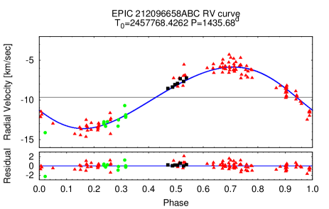
Figure 7: RV curve of the centre-of-mass ABC corresponding to the outer orbit with $P_{3}=3.9$ yr. Red triangles plot the CfA RVs, black squares – CHIRON RVs, green circles – other RVs. Blue line represents the RV curve calculated from the spectro-photodynamical solution. The residuals to this solution are shown in the bottom panel.

A plot of $V_{0}$ vs. time clearly shows its variation with a period of $\sim$4 years; three cycles between 1999.3 and 2019.0 are covered. The preliminary orbital elements describing the $V_{0}(t)$ variation are given in Table 3, the RV curve is plotted in Fig. 7. The RV amplitude in the outer orbit is denoted by $K_{5}$. We adopted the erors of 1 km s^-1 for the CfA data, 0.5 km s^-1 for TRES, VUES and UVES, and 0.1 km s^-1 for CHIRON. The latter RVs are distinguished by the tight sequence of black squares around the phase 0.5, showing the $V_{0}$ trend in just two months. The global weighted rms residuals are 0.38 km s^-1 . The long and extensive coverage of the CfA data is essential for constraining the outer orbit.

Table 3: Elements of the outer orbit

Element	Value
$P_{3}$ (d)	1427$\pm$5
$\tau_{3}$ (BJD $-$2400000)	51786$\pm$102
$e_{3}$	0.068$\pm$0.022
$\omega_{3}$ (deg)	52$\pm$27
$K_{5}$ (km s-1 )	3.963$\pm$0.15
$\gamma$ (km s-1 )	$-$9.82$\pm$0.10

The middle and inner orbits computed from the CfA data of 2007–2008 happen to be near the maximum of the RV curve in Fig. 7, hence $\gamma_{\rm CfA}=-6.4$ km s^-1 ; the trend during this period was small. Similarly, most VUES observations cover the minimum of this curve, hence $\gamma_{\rm VUES}=-12.2$ km s^-1 (the first VUES observation does not match the inner orbits without an offset correction).

Given that the inner pair is eclipsing, the factor $\sin^{3}i_{\rm A,B}\approx 1$, so the spectroscopic masses are close to the true masses of the components. The mass sum of 1.9 ${\cal M}_{\odot}$ for A+B+C and the RV amplitude of the outer orbit then lead to $M_{D}>0.36$ ${\cal M}_{\odot}$ . If the inclination of the outer orbit were substantially different from $90^{\circ}$, the large resulting $M_{D}$ would contradict its non-detection in the spectra, so we adopt $M_{D}=0.4$ ${\cal M}_{\odot}$ (this is confirmed below by the full modelling). The total mass and the period define the semimajor axis of the outer orbit, 3.26 au or 67 mas on the sky.

At the Gaia DR2 epoch, 2015.5, the star D was receding from ABC, moving toward maximum separation. The projected speed of the mean orbital motion during the time interval of 2015.5$\pm$0.5 years was $\mu_{\rm orb}=40$ mas yr^-1, directed away from the primary. Comparing this speed to the observed $\Delta\mu=7.0$ mas yr^-1 and neglecting the light of the star D allows a direct measurement of the outer mass ratio $q_{3}$ from the relation $\Delta\mu/\mu_{\rm orb}=q_{3}/(1+q_{3})$. Hence, $q_{3}=0.21$ and $M_{D}=0.40$ ${\cal M}_{\odot}$ . This confirms our assumption that the outer orbit has a large inclination. The direction of $\Delta\mu$ suggests that the companion D was at the position angle of $\sim 80^{\circ}$ in 2015.5. Without actually resolving the outer binary, we already know approximately all its orbital elements and can compute the positions.

4 Dynamical modelling

As a consequence of the compactness of this quadruple system (the period ratios are $P_{2}/P_{1}\sim 20.2$ and $P_{3}/P_{2}\sim 24.4$) the orbital motions of the four stars depart significantly from pure Keplerian orbits. Therefore, the accurate modelling of all observations needs a spectro-photodynamical approach, i. e. the combination of the simultaneous analysis of the RVs and photometric data with the numerical integration of the four-body motion. This analysis was carried out with the software package Lightcurvefactory (see Borkovits et al., 2019, and further references therein) of which the latest version is now able to handle quadruple systems both in 2+2 and 2+1+1 configurations. The relevant modifications of the orbital equations to be numerically integrated in this new version are discussed in Appendix A.

Apart from the inclusion of the fourth star forming the third, outermost “binary” with the centre of mass of the ABC components, this complex analysis was carried out in a very similar manner as described in Sect. 7 of Borkovits et al. (2019) and, therefore, here we discuss only the basic steps briefly. We carried out a joint Markov Chain Monte Carlo (MCMC) parameters search for the following data series:

• Two sets of long cadence K2 lightcurves;

• The RVs of components A, B, and C;

• The ETV curves of the innermost EB (for both primary and secondary minima).

Regarding item (i), we consider two variants of processed K2 lightcurves, with constant and variable eclipse depth, as described in Sect. 2.1.1. In both cases, we use only a narrow window of width $\sim 0.12$ d centered on each eclipse (blue points in Fig. 2, right panel). The out-of-eclipse brightness variations are negligible, and the omission of these data saves a significant amount of computational time. Most dynamical information coded in the lightcurves is contained in the fine structure and timings of the eclipses. Note also, that for the $\sim 29.4$-min long-cadence time of Kepler, we apply a cadence time correction on the model lightcurves (see Borkovits et al., 2019, for details). Considering that the eclipse depth variation in the Kepler data has been confirmed by our ground-based photometry, we discuss below only the uneven eclipse depth solution.

Turning to the RV curves, we emphasize that instead of fitting the usual analytical formulae, our numerical integrator calculates for all time instances the 3D velocity vectors of all four bodies, the $v_{z}$ components of those vectors give directly the RVs relative to the centre of mass of the quadruple system. The systemic velocity, $\gamma$, is then calculated a posteriori by a simple linear regression minimizing the $\chi^{2}_{\mathrm{RV}}$ residuals between measured RVs and the model. We found only minor zero-point differences amongst the RV instruments (see Sect. 2.2) and neglected them.

In principle, the K2 lightcurves carry the same timing information as the ETV curves, making the latter redundant. However, the advantages of using both the lightcurves and the ETV curves together have been explained in Borkovits et al. (2019). Similarly to our previous work, the ETV curves were used to preset the period ($P_{1}$) and phase term $(\mathcal{T}_{0})_{1}$ of the innermost binary for each new set of the trial parameters. The latest ETV points from the ground-based photometry were also added to the data set.

During our analysis, we carried out several dozens of MCMC runs and tried different sets and combinations of adjustable parameters. We also applied some additional relations to constrain some of the parameters in order to reduce the degrees of freedom in our problem. For example, while the masses of all four stars can be deduced from the joint dynamical analysis of the ETV and RV curves and, combining these results with the outputs of the lightcurve analysis, the physical dimensions of the eclipsing stars can also be determined, none of the observational data used for the photodynamical modelling carry information on the radii of the stars C and D. Similarly, only the temperature ratio of stars B and A ($T_{\mathrm{B}}/T_{\mathrm{A}}$) can be constrained by the light curve, while the effective temperature of one star in the inner binary should be taken from an external source. The photodynamical model can say nothing on the effective temperatures of the stars C and D. Their net flux in the Kepler band is manifested only as extra flux for the lightcurve model. In order to get reliable information on these parameters we applied different options. Regarding $T_{\mathrm{A}}$, in some runs we constrained it with a Gaussian prior centered to the temperature given in Gaia DR2 ($T_{\mathrm{eff}}=3978$ K), while in another series of runs the code calculated internally the temperature in each trial step from the stellar mass $m_{\mathrm{A}}$ with the use of the mass–temperature relations of Tout et al. (1996), valid for zero age main sequence (ZAMS) stars. During our analysis the radii of the two outer stars ($R_{\mathrm{C,D}}$) and also the effective temperature of the star D ($T_{\mathrm{D}}$) were also connected internally to their masses via the relations of Tout et al. (1996). (For these calculations solar metallicity was assumed.) Applying these three constraints, the fourth remaining parameter, i. e. $T_{\mathrm{C}}$, takes the role of the extra light parameter ($l_{\mathrm{x}}$) and, therefore, there is no need to use this latter one.

Besides the above mentioned constraints, in most of our runs we adjusted the following parameters:

• Three parameters related to the orbital elements of the inner binary: eccentricity ($e_{1}$), the phase of the secondary eclipse relative to the primary one ($\phi_{\mathrm{sec,1}}$) which constrains the argument of periastron ($\omega_{1}$, see Rappaport et al. 2017), and the inclination ($i_{1}$);

• Two times six parameters related to the orbital elements of the middle and the outermost orbits: $P_{2,3}$, $(e\sin\omega)_{2,3}$, $(e\cos\omega)_{2,3}$, $i_{2,3}$, the times of the periastron passages of stars C and D along their revolutions on the middle and the outermost orbits, respectively ($\tau_{2,3}$), and the position angles of the nodes of the two orbits ($\Omega_{2,3}$);

• Four mass-related parameters: the mass of the component A, $m_{\mathrm{A}}$, and the mass ratios of all three orbits $q_{1,2,3}$;

• and, finally, four other parameters which are related (almost) exclusively to the lightcurve solutions, as follows: the duration of the primary eclipse $(\Delta t)_{\mathrm{pri}}$ closest to epoch $t_{0}$ (which is an observable that is strongly connected to the sum of the fractional, i. e. scaled by the inner semi-major axis, radii of stars A and B, see Rappaport et al. 2017), the ratio of the radii of stars A and B ($R_{\mathrm{B}}/R_{\mathrm{A}}$), and the temperature ratios of $T_{\mathrm{B}}/T_{\mathrm{A}}$ and $T_{\mathrm{C}}/T_{\mathrm{A}}$.

Turning to other, lightcurve-dependent parameters, we applied a logarithmic limb-darkening law, where the coefficients were interpolated from the pre-computed passband-dependent tables in the Phoebe software (Prša & Zwitter, 2005). The Phoebe-based tables, in turn, were derived from the stellar atmospheric models of Castelli & Kurucz (2004). Due to the nearly spherical stellar shapes in the inner binary, an accurate setting of gravity darkening coefficients has no influence on the lightcurve solution and, therefore, we simply adopted a fixed value of $g=0.32$ which is appropriate for late-type stars according to the traditional model of Lucy (1967). We also found that the illumination/reradiation effect was quite negligible for the eclipsing binary; therefore, in order to save computing time, this effect was neglected. On the other hand, the Doppler-boosting effect (Loeb & Gaudi, 2003; van Kerkwijk et al., 2010) was included into our model. Furthermore, in the absense of any other information, we assumed that the equatorial planes of stars A and B are aligned with the innermost orbital plane. The projected rotational velocities of stars A, B and C were set to their spectroscopically obtained values (see Sect. 2.2.3).

The orbital and astrophysical parameters derived from the ‘uneven eclipse depth scenario’ spectro-photodynamical analysis are tabulated in Table 4, and will be discussed in the subsequent Sections 5 and 6. The corresponding model lightcurves are presented in Fig. 2, while the different RV curves are shown in Figs. 6, 7, and 8. Finally, the model ETV curve plotted against the observed ETVs is shown in Fig. 3.

Table 4: Orbital and astrophysical parameters from the joint photodynamical lightcurve, three RV curves and ETV solution

orbital elementsa
	subsystem
	A–B		AB–C	ABC–D
$P$ [days]	$2.93001\pm 0.00008$		$59.157\pm 0.006$	$1441.4\pm 10.7$
$a$ [R⊙]	$9.259\pm 0.054$		$78.77\pm 0.48$	$700.9\pm 6.7$
$e$	$0.00873\pm 0.00005$		$0.2781\pm 0.0040$	$0.0814\pm 0.0034$
$\omega$ [deg]	$175.96\pm 6.32$		$332.87\pm 0.51$	$293.04\pm 2.87$
$i$ [deg]	$87.725\pm 0.032$		$86.528\pm 0.136$	$84.170\pm 5.073$
$\tau$ [BJD - 2400000]	$57142.7234\pm 0.0515$		$57123.285\pm 0.089$	$57768.4\pm 10.1$
$\Omega$ [deg]	$0.0$		$-1.797\pm 0.088$	$-21.422\pm 16.598$
$i_{\mathrm{m}}$ [deg]	$-$		$2.157\pm 0.107$	$21.658\pm 16.345$
mass ratio $[q=m_{\mathrm{sec}}/m_{\mathrm{pri}}]$	$0.983\pm 0.009$		$0.511\pm 0.009$	$0.186\pm 0.019$
$K_{\mathrm{pri}}$ [km s-1]	$79.217\pm 0.593$		$23.687\pm 0.318$	$3.861\pm 0.333$
$K_{\mathrm{sec}}$ [km s-1]	$80.599\pm 0.599$		$46.353\pm 0.404$	$20.706\pm 0.428$
$\gamma$ [km s-1]	$-$			$-9.608\pm 0.129$
stellar parameters
	A	B	C	D
Relative quantities
fractional radius [$R/a$]	$0.0635\pm 0.0012$	$0.0622\pm 0.0012$	$0.0075\pm 0.0002$	$0.00048\pm 0.00004$
fractional flux [in Kepler-band]	$0.3232$	$0.2867$	$0.3550$	$0.0351$
Physical Quantities
$m$ [M⊙]	$0.625\pm 0.010$	$0.614\pm 0.012$	$0.633\pm 0.016$	$0.349\pm 0.036$
$R$ [R⊙]	$0.588\pm 0.012$	$0.576\pm 0.012$	$0.590\pm 0.015^{b}$	$0.336\pm 0.025^{b}$
$T_{\mathrm{eff}}$ [K]	$4043\pm 60^{c}$	$3986\pm 60$	$4064\pm 83$	$3373\pm 159^{c}$
$L_{\mathrm{bol}}$ [L⊙]	$0.0829\pm 0.0060$	$0.0753\pm 0.0055$	$0.0852\pm 0.0078$	$0.0131\pm 0.0032$
$M_{\mathrm{bol}}$	$7.44\pm 0.08$	$7.55\pm 0.08$	$7.41\pm 0.10$	$9.44\pm 0.26$
$M_{V}$	$8.50\pm 0.11$	$8.69\pm 0.12$	$8.44\pm 0.14$	$12.24\pm 0.73$
$\log g$ [dex]	$4.70\pm 0.02$	$4.71\pm 0.02$	$4.70\pm 0.03$	$4.93\pm 0.08$
$(M_{V})_{\mathrm{tot}}$	$7.34\pm 0.07$
distanced [pc]	$<50.2\pm 1.7$

Notes. $a$: Instantaneous, osculating orbital elements, calculated for epoch $t_{0}=2457143.395$ (BJD); $b$: Calculated from the mass–radius relations of Tout et al. (1996); $c$: Calculated from the mass–temperature relations of Tout et al. (1996); $d$: Photometric maximum distance, see text for details.

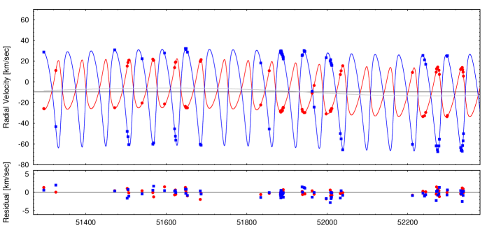
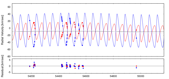
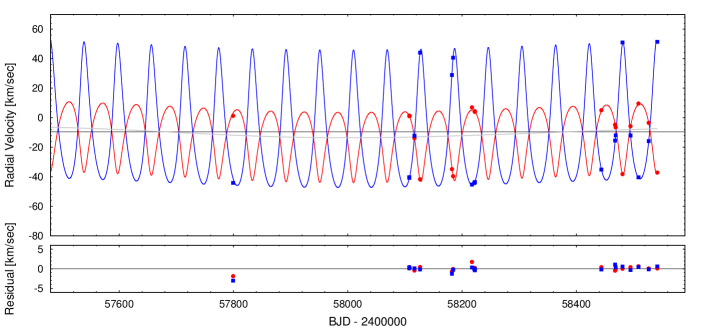
Figure 8: 1100-day-long sections of RV data, model solution, and residuals. For better visibility, we do not plot the RVs of the innermost pair. Red circles denote the mass-weighted average of the observed RVs of stars A and B (i. e. the “observed” RV of their barycentre), while blue boxes stand for the directly observed RV data of star C. Red and blue lines show the appropriate model RV curves. Furthermore, grey line represent the outermost orbit RV component, while thin black line stands for the constant $\gamma$ velocity. Note variations both in the shape and orientation of the RV orbits. These are consequences of the quick apsidal motion of the middle orbit due to the strong dynamical interactions of the four stars.

As a sanity check for the photodynamical solution, we calculate the maximum photometric distance of HIP 41431 by combining the total $V$ magnitude of the system (see the penultimate row in Table 4) with the apparent $V$ magnitude (see Table 1). This results in a photometric distance of $d_{\mathrm{phot}}\leq 50\pm 2$ pc, which is in good agreement with the Gaia parallax.

5 Physical parameters of the components

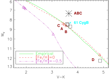
Figure 9: Color-magnitude diagram. The lines are 1-Gyr isochrones from Bressan et al. (2012) for metallicity [Fe/H] of 0 and $-0.5$ dex and the empirical relations of Pecaut & Mamajek (2013). Squares show the components, the triangles are isochrone locations corresponding to the measured masses, the large asterisk is the combined light of all stars. The location of the nearby K7V dwarf 61 Cyg B is shown by the blue star.

The masses obtained from the spectro-photodynamical model are in good agreement with masses deduced from the preliminary RV analysis and the Gaia astrometry (Sect. 3). Similarly, the relative fluxes of the visible stars A, B, and C in the $V$ band deduced from the model, 0.95:0.79:1, match well their relative fluxes measured spectroscopically (see Sect. 2.2.1). The minor contribution of the faint star D to the $V$-band flux is accounted for by assuming that it is an MS dwarf. The $V-K$ colors of the stars are computed from their effective temperatures listed in Table 4 using standard relations for MS stars (e.g. Pecaut & Mamajek, 2013) and adjusted to match the measured combined $V-K_{s}$ color in Table 1. This allows us to place the stars on the color-magnitude diagram (CMD) in Fig. 9 using the Gaia parallax.

The masses, colors, and absolute magnitudes of the visible stars A, B, and C match well both the empirical relations of Pecaut & Mamajek (2013) and the theoretical isochrone for solar metallicity, while the star D of 0.35 ${\cal M}_{\odot}$ contributes only 0.01 to the total light in the $V$ band and 0.35 in the Kepler band. The empirical relations of Benedict et al. (2016) for M-type dwarfs predict the $V-K$ colors from 3.61 to 3.66 mag for stars with masses of the components A, B, and C, and match the observed combined color $V-K_{s}=3.65$ mag. The observed absolute $V$ magnitudes are brighter than those of Benedict et al. by $\sim$0.3 mag, either because these stars are slightly evolved or because of the reduced blanketing owing to sub-solar metallicity. The stars A, B, C have effective temperature close to 4000 K or slightly lower (Gaia gives $T_{\rm eff}=3978$ K) and gravity $\log g=4.7$ in cgs units. The PARSEC isochrone for [Fe/H]=$-0.5$ (Palacios et al., 2010), on the other hand, corresponds to bluer and brighter stars (for the same masses) and contradicts the observations. The discrepancy between theoretical isochrones and actual colors of low-mass stars has been recently noted by Howes et al. (2019). They discuss the “benchmark” K7V star 61 Cyg B (HD 201092) as an example. Its parameters and position on the CMD happen to be similar to the components A, B, and C of HIP 41431. The measurements of [Fe/H] for the 61 Cyg A and B listed in Simbad have a large scatter, illustrating the difficulty of the spectroscopic analysis of late-type dwarfs. Most measurements give [Fe/H]$\approx-0.4$ dex for 61 Cyg, and the metallicity of HIP 41431 is likely similar, i. e. mildly sub-solar.

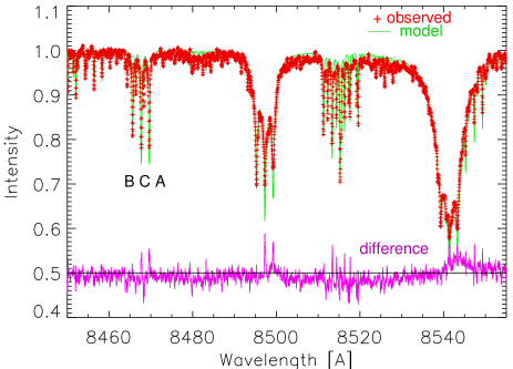
Figure 10: Observed spectrum (red crosses) is compared to the synthetic spectrum with $T_{\rm eff}=4000$ K, $\log g=4.7$, and [Fe/H]=$-$0.5 dex (green line) around the CaII near-infrared triplet. The magenta line shows the difference. The components’ order (left to right) is B, C, A.

Stellar parameters can be measured directly from the high-resolution spectra if the spectra of individual components are isolated (disentangled). This approach was implemented for the CHIRON spectra, but even by combining them all and averaging the component’s spectra, the signal to noise ratio (SNR) remains modest. Alternatively, we can compute the triple-lined synthetic spectrum and compare it to the observed one. The spectrum of HIP 41431 with the largest SNR was taken on 2017 December 29 (JD 2458116.697) with UVES (see Sect. 2.2.4). Using the measured RVs and relative fluxes, we shift and scale the synthetic spectrum to model the triple-lined system. Such forward-modelling avoids the need to disentangle the observed spectrum. A small correction for the estimated dilution by the light of the star D is applied.

Figure 10 shows a fragment of the near-IR UVES spectrum compared to the synthetic spectrum from the Pollux library (Palacios et al., 2010). We made this comparison for the [Fe/H] values ranging from $-1$ to $+0.5$ dex and found the best match for [Fe/H]=$-$0.5 dex. Note that the effective temperature of the synthetic spectrum differs slightly from the estimated stellar temperatures, but synthetic spectra of dwarfs with lower temperatures are not available in the Pollux library.

We tried to find the spectral signature of the faint star D by correlating the difference between the UVES spectrum and its triple-lined model with the synthetic spectra of different $T_{\rm eff}$ or with a binary mask, near the CaII infrared triplet. The resulting correlation function does not contain the expected details. The star D could have a fast rotation or could be a close spectroscopic pair.

6 Orbital properties and dynamical evolution

As mentioned previously, the four stars in this compact quadruple system interact dynamically and therefore, the three orbits are subjected to strong and fast dynamical perturbations. Spectacular manifestations of these interactions are nicely visible even on the four-year-long data train of the measured ETVs (Fig. 3) of the innermost, eclipsing pair.

First, we note the 59-day sine-like modulation of the ETV, similar (but not identical) for the primary and secondary ETVs. The dominating contributor to this modulation is the third-body perturbation from the star C that alternates the mean motion (and also the orbital elements) of the innermost binary on the timescale of the period of the middle orbit (Borkovits et al., 2015). The contribution of the classic light-travel time effect (LITE) to this 59-day variation is only about 10%.

Second, the crossing of the two ETV curves reveals a fast, dynamically forced apsidal motion. According to our numerical integration, which was a substantial part of the photodynamical solution, during this four years the major axis of the innermost orbit has turned by $\approx 150-160\degr$, i. e., has made almost half a revolution (see Fig. 11). Therefore, the current period of the apsidal motion of the innermost orbit is $U_{1}\approx 9$ yr. Only two binaries formed by non-degenerate stars with shorter apsidal motion periods are known to date. These are the inner binaries of the compact hierarchical triple systems KOI-126 and KIC 05771589, reported by Carter et al. (2011) and Borkovits et al. (2015), respectively.

Finally, the $P_{3}\sim 3.9$ yr LITE induced by the outermost component is also present.

At this point we have to note, that the ETV residuals (Fig 3, lower panel) show small, but systhematic departures in the order of some $10^{-4}$ days around BJD 2 458 150 and 2 458 520, i. e. during the late campaign (C16 and C18) observations of the K2 mission. In this moment we cannot decide whether these small, but systhematic discrepancies, which however do not exceed the estimated accuracies of the individual ETV points have physical origins indicating some inaccuracies in the parameters of the expected four-body model, or they are consequences of some instrumental effects.

Turning to the RV data, a more spectacular, and almost uniquely observed manifestation of the apsidal rotation of the middle orbit can be seen in Fig. 8, where we plot the RVs of the three visible stars A, B, and C (after subtracting the orbit of the eclising pair), together with the corresponding spectro-photodynamical model for the whole, 20-year-long time span of our observations. The apsidal rotation of the middle orbit results in the notable variation of the shape of the RV curves.

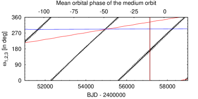
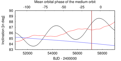
Figure 11: Variations of the osculating (observable) arguments of periastron ($\omega_{1,2,3}$) and inclinations ($i_{1,2,3}$) of the three orbits between 1998.5 and 2020.4, as calculated from our spectro-photodynamical solution. Black, red and blue lines denote the orbital elements of the innermost, middle and outer orbits, respectively. The elements are averaged for the period of the corresponding orbits. Vertical brown line represents the beginning of the Kepler observations.

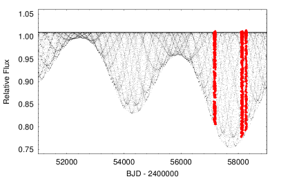
Figure 12: The model lightcurve of the star between 1998.5 and 2020.4 (thin black curve). The eclipse depth variations caused by the orbital plane precession are well visible. The K2 lightcurves collected during Campaigns 5, 16 and 18 are also plotted with red circles.

Orbital inclination is another key observable in an eclipsing binary. Our photodynamical solution has revealed small, but definitely non-zero relative (mutual) inclination between the two inner orbital planes: $i_{\mathrm{mut1-2}}=2\aas@@fstack{\circ}2\pm 0\aas@@fstack{\circ}1$. The mutual inclination between the outermost and the inner and middle orbits is larger, although its uncertaintly is substantial: $i_{\mathrm{mut1-3}}=22\degr\pm 16\degr$ and $i_{\mathrm{mut2-3}}=20\degr\pm 16\degr$. The non-coplanarity of the orbits triggers precession of all three orbital planes, illustrated in the right panel of Fig. 11, where the variations of the three observable orbital inclinations (i. e. the angles between the orbital planes and the plane of the sky) are plotted.

While the dynamical effects of such orbital misalignments are expected to occur only on very long times scales, their observational consequences, however, are manifested almost promptly, in dramatic eclipse depth variations. In Fig. 12 we plot the model lightcurve of the system since the beginning of the spectroscopic observations. The $\approx 9.2$ year period cyclic variation of the eclipse depths which, naturally, correlates with the $\Delta i_{1}\approx 3.5\degr$ amplitude, short-term variation of the inclination ($i_{1}$) of the innermost orbit, is clearly visible. Moreover, another (on this timescale linear) effect is also well visible; it corresponds to the longer time-scale and larger-amplitude precession triggered by the more inclined outermost orbit. As a consequence, if the photodynamical solution is correct, in the forthcoming decades one can expect that the mean visible inclinations of the innermost and middle orbits (i. e., $i_{1}$ and $i_{2}$ averaged over the $\approx 9.2$ yr-period of the short-term precession) and, therefore, the averaged eclipse depths will increase. Moreover, when these inclinations reach $\approx 90\degr$ around 2040, eclipses of the component C should also become observable for several years.

We emphasize, however, that the relative nodal angle of the outermost orbit ($\Omega_{3}$) is obtained only with a large uncertainty and thus, the corresponding two outer mutual inclinations are only weakly constrained. Therefore, these results should be considered as tentative. The reason of this uncertainty is that only the eclipse depth variation of the eclipsing pair is strongly sensitive to the rate of the (visible) inclination variation of the innermost pair and, therefore, only the K2 observations, which cover a small fraction of the $\approx 1260$ day-long interval contain really conclusive information about the several hundred-year-long outer precession cycle. Moreover, as discussed in Sect. 2.1.1, the reality of the eclipse depth variations observed by Kepler might be debatable. Therefore, follow-up observations and continuous monitoring of the eclipse depth variations are crucial.

We added this star to the long-term eclipse monitoring programme of Baja Observatory, Hungary, as a top priority target. Unfortunately, due to the bad weather conditions (which are usual in the winter season), so far we were able to observe only four primary and two secondary eclipses. Furthermore, owing to the poor sky conditions, two primary minima were observed in unfiltered mode, and only four eclipses were observed with a standardized Kron-Cousins $R_{C}$ filter. Normally, unfiltered minima observations are useful for the times of minima determination but unfit for studying the eclipse depth variation. Therefore, we consider only the $R_{C}$-band eclipse observations. We generated the $R_{C}$-band model lightcurve for those nights and compared it to the observations (see Fig. 13). As one can see, the agreement for the primary eclipse is almost perfect. For the secondary eclipse, a minor systematic deviation can be seen. However, the decrease of the eclipse depths is beyond doubt. This fact confirms not only the ongoing precession of the innermost orbit but, retrospectively, justifies the physical origin of the eclipse depth variations observed in the different K2 campaigns.

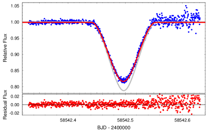
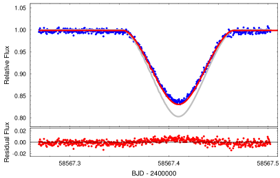
Figure 13: Upper left panel: Primary eclipse of HIP 41431 measured in $R_{C}$-band on the night of 27/28 Feb 2019 (blue circles) and the corresponding photodynamical model lightcurves both for the uneven and uniform K2 eclipse depths scenarios (red, and grey lines, respectively). As one can see, the measured eclipse depth is in perfect agreement with the predictions of the uneven eclipse depths scenario and therefore, it confirms the physical origin of the eclipse depth differences amongst the different K2 campaigns. Upper right panel: The same for the secondary eclipse measured also in $R_{C}$-band on the night of 24/25 March 2019. Lower panels: Observations vs. uneven eclipse depth model lightcurve residuals.

In order to check the long time-scale dynamical evolution and stability of our quadruple system, we carried out further numerical integration on a timescale of $10^{8}$ yr. The integrator was the same as in the case of the photodynamical analysis. Therefore, beyond the four-body point-mass forces, tidal forces acting upon in the innermost binary were also considered, including the Eulerian equations of the rotations of stars A and B. Furthermore, for some additional runs tidal dissipation (within the framework of the equilibrium tide approximation), and relativistic apsidal motion were also included (see Appendix A for details). The additional parameters necessary for these integrations were set as follows. The inner structure (or apsidal motion) constants of both stars A and B were set to $k_{2}=0.02$ which, according to Torres et al. (2010), is appropriate for such low-mass stars. Furthermore, the dissipation rates for both stars were set to $\lambda=2\times 10^{-5}$. This type of dissipation rate was defined by Eq. (13) in Kiseleva et al. (1998). It is connected to the small tidal lag time through the formula:

$$\Delta t=-\frac{3}{8}\sqrt{\frac{R^{3}}{Gm}}\left(1+2k_{2}\right)^{2}\lambda$$ (2)

(see Borkovits et al., 2004, Eq. 25). The choosen numerical values of $\lambda$ correspond to tidal lags of $\Delta t\approx-2\times 10^{-10}$ days for both stars. The integrations did not reveal any dramatic variations in the orbital elements of the three orbits. Therefore, we conclude that the orbital configuration is stable up to the nuclear evolution time scales.

On the other hand, the numerical method allows us to study the spin evolution of the innermost two stars. This is especially interesting in the present case, as the most unusual characteristic of this system is the slow axial rotation of the stars comprising the inner pair. For HIP 41431, the standard assumption that the axes are perpendicular to the orbit is not trivial. The likely non-coplanarity of the outermost orbit forces significant orbital plane precession, which may lead to spin-orbit misalignement, as suggested e. g. by Beust et al. (1997) in the case of TY CrA. Furthermore, as found by Correia et al. (2016), the secular evolution of the spins in hierarchical triple systems when viscous tidal forces are present might be affected strongly by secular resonances between orbital and spin precessions and, therefore, chaotic rotation might occur.

In what follows we discuss briefly some results of three different integrator runs. Dissipative forces were taken into account in all three runs. For the run ‘A’, the spin axes of stars A and B are parallel to the orbital spin vector of the innermost orbit at the epoch $t_{0}$ used in the photodynamical model. Furthermore, the spin rates are set according to the spectroscopically measured projected rotation velocities. In other words, apart from the dissipation terms, this numerical integration is a simple extention of the accepted photodynamical model over a much longer time scale. For the run ‘B’, the initial orbital elements were the same, but the orientation and magnitude of stellar spins are set arbitrarily. Finally, for the run ‘C’, the initial parameters are the same as in run ‘A’, but the outermost, fourth body is removed, i. e., a three-body integration was carried out.

In Fig. 14 we plot the variations of the orbital inclinations of the innermost orbit and of the equatorial planes of stars A and B on different time scales. The $\Delta i_{1}\approx 30\degr$ peak-to-peak amplitude, $\approx 600$-year-period orbital precession triggered by the inclined outermost orbit is well visible. The short-term observational consequences of this additional precession were briefly discussed a few paragraphs above. As our results illustrate, this orbital plane precession triggers the stellar spin precession with an initially similar amplitude. However, the equatorial planes of the stars are unable to follow strictly the orbital plane, as shown in Fig. 15. As a consequence, the stellar equators no longer remain aligned to the continuously varying orbital plane. On the other hand, due to the dissipative forces the amplitude of the spin precession dumps quickly in the first few hundred thousand years. Dramatic changes occur, however, during the later stages of the evolution. The origin of these changes can be found in some kind of spin-orbit resonances. We plot the evolution of the stellar spin rates in Fig. 16. As one can see, due to the dissipative forces the originally sub- or super-synchronous rotation periods quickly relax to the orbital period. However, in this case various spin-orbit resonances may occur. As a consequence, the stellar spins can again desynchronize and, furthermore, large amplitude equatorial plane precession may also happen. The investigation of these phenomena is beyond the scope of the present paper; they were studied, e. g., by Correia et al. (2016). In the context of the present paper, we conclude that the measured low projected rotational velocities of stars A and B probably offer observational evidence for the presence of strong spin-orbit coupling. The question whether the stars have strongly inclined spin axes or rotate slowly (or both) cannot be answered at present.

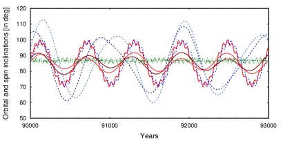
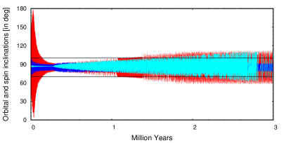
Figure 14: The evolution of the orbital inclination of the innermost binary and the orientation of the stellar equators of stars A and B during three different integration runs. Left panel: A 3000-year-long zoom into the variation of the angles. Solid lines (with three different shades of red) represent the variation of the orbital inclination and the equatorial angles of the two stars during run ‘A’. The short-period, small amplitude fluctuations in the inclination reflects the precession due to the star C, while the longer period, larger amplitude variation is the precession caused by the star D. Dotted lines (in blue colors) show the same parameters for the run ‘B’ (i.e. inclined spin axes), while the dash-dotted green lines represent run ‘C’, i.e. the originally aligned 3-body model. Right panel: 3 Myr-long evolution of the orientation of the stellar equators. For clarity, we plot only one star for each run. Blue: star A in run ‘A’ (aligned); red: star B in run ‘B’ (inclined); cyan: star A in run ‘C’ (aligned three-body). Horizontal black lines stand for the maximum and minimum values of the orbital inclination of the precessing innermost orbit.

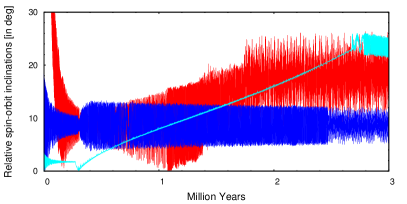
Figure 15: The variation of the mutual inclination angles between the innermost orbital plane and stellar equators during 3 Myr. Blue: star A in run ‘A’ (aligned); red: star B in run ‘B’ (inclined); cyan: star A in run ‘C’ (aligned three-body).

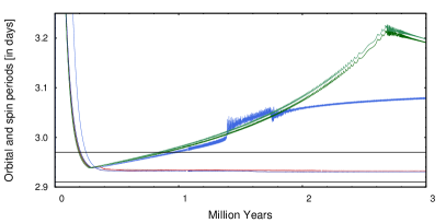
Figure 16: 3 My-long evolution of the stellar spins of the innermost binary members. Two (undistinguishable) red curves stand for the spin periods of stars A and B during run ‘A’ (aligned axes). Darker and lighter blue lines represent spin periods of star A and B, respectively, in run ‘B’ (inclined stellar axes). Furthermore, darker and lighter green curves denote the spin periods of stars A and B in run ‘C’ (aligned 3-body model). Finally, horizontal black lines show the upper and lower values of the fluctuating osculating orbital period of the innermost orbit. One can see that due to dissipative forces the spin periods quickly reach the orbital period. However, in this quasi-synchronized state different spin-orbit coupling and resonances may occur.

7 Discussion and conclusions

The triple system HIP 41431 is remarkable in several respects. First, it is very compact, with a 3-tier (3+1) hierarchy fitting inside the 3.3-au outer orbit. Second, all orbits are close to one plane (mutual inclinations of 2$\aas@@fstack{\circ}$2$\pm$0$\aas@@fstack{\circ}$1 and 21°$\pm$16°), while the period ratios are similar (20.17 and 24.4). The orbits interact dynamically.

The spatial velocity of this system $(U,V,W)=(8.1,7.7,-1.4)$ km s^-1 does not distinguish it from the old disk population and does not match known kinematical groups of young stars in the solar neighbourhood. The spectra do not have the lithium 6708Å line or emissions in H$\alpha$ typical of young stars and no variability associated with chromospheric activity or star spots was found in the K2 data. We conclude that this multiple system is not young.

The most unusual characteristic of this system is the slow axial rotation of stars comprising the short-period inner pair, expected to be tidally synchronzed. However, this apparent paradox might be caused by the spin-orbit coupling and resonances triggered by the dynamically interacting third and fourth stellar companions, leading to chaotic rotation.

We looked for similarly compact hierarchies in the Multiple Star Catalog (MSC) (Tokovinin, 2018a) . The current version of the catalog contains 29 triples with outer periods $P_{\mathrm{out}}<150$ d (not counting the present system). All MS triples except one have primary components of earlier spectral type than HIP 41431 (likely an observational selection effect). There are only six known triples, however, with the outer periods shorter than 59 d. While the absolute dimensions of the orbits (and, therefore, the orbital periods) are very important parameters from the point of view of the effectiveness of the tidal forces and also of the system formation scenarios, the period ratios are more significant indicators of the strength of dynamical interactions between orbits. In this regard, the period ratios of $\sim$20 found in the two subsystems of HIP 41431 are far from being extreme. In the small mutual inclination regime, such period ratios are well within the stability region of hierarchical triple stars (see, e. g. Mardling & Aarseth, 2001).

No quadruple systems of 3+1 hierarchy as compact as HIP 41431 were known previously. However, there are at least three compact triple systems with short outer periods among the Kepler’s prime misson EBs where the systematic residuals of the four-year-long ETV data might indicate the presence of a fourth component (Borkovits et al., 2016).

Our work has contributed an interesting system that challenges the theories of star formation. Compact and coplanar hierarchical stellar systems like HIP 41431 are probably a result of migration in massive disks that are present at the time of star formation. The first two stellar embryos condense from gas, accrete mass, and migrate inward, while outer components condense later in the same accretion flow (e. g. by disc fragmentation) and, in their turn, migrate inward. No other scenario can plausibly explain the origin of such well-organized, planetary-like hierarchies. However, further discussion of formation mechanisms is beyond the scope of this paper.

Appendix A Some details of the numerical integrator for modelling 2+1+1 hierarchies

As it was mentioned above, the numerical integrator which was used in the spectro-photodynamical code is an upgraded version of the 3-body integrator described in Borkovits et al. (2004). Further details of the practical implementation of a numerical integrator coupled to the lightcurve emulator were discussed in the appendix of Borkovits et al. (2019). Here we discuss the additional modifications introduced into the code to handle quadruple systems with 3+1 hierarchy.

Similar to the previous hierarchical triple star case, the Jacobian vector formalism is consistently used. In order to describe the motion of the fourth body and its effect on the inner three stars, now we introduce the third Jacobian vector which points to the outermost component (star D) from the centre of mass of the inner triple subsystem (stars A, B, and C).

Let us denote by $\vec{r}_{i}$ the barycentric radius vector of the component $i$ and by $\vec{r}_{ij}=\vec{r}_{j}-\vec{r}_{i}$ the vector between components $j$ and $i$. Then, the first three Jacobian vectors are as follows:

$$\vec{\rho}_{1} = \vec{r}_{12},$$ (3)

$$\vec{\rho}_{2} = \vec{r}_{3}-\frac{m_{1}}{m_{12}}\vec{r}_{1}-\frac{m_{2}}{m_{12}}\vec{r}_{2}=\vec{r}_{13}-\frac{m_{2}}{m_{12}}\vec{r}_{12}=\vec{r}_{23}+\frac{m_{1}}{m_{12}}\vec{r}_{12},$$ (4)

$$\vec{\rho}_{3} = \vec{r}_{4}-\frac{m_{1}}{m_{123}}\vec{r}_{1}-\frac{m_{2}}{m_{123}}\vec{r}_{2}-\frac{m_{3}}{m_{123}}\vec{r}_{3},$$ (5)

while the mutual distances between the components are:

$$\vec{r}_{12} = \vec{\rho}_{1},$$ (6)

$$\vec{r}_{13} = \vec{\rho}_{2}+\frac{m_{2}}{m_{12}}\vec{\rho}_{1}$$ (7)

$$\vec{r}_{14} = \vec{\rho}_{3}+\frac{m_{2}}{m_{12}}\vec{\rho}_{1}+\frac{m_{3}}{m_{123}}\vec{\rho}_{2}$$ (8)

$$\vec{r}_{23} = \vec{\rho}_{2}-\frac{m_{1}}{m_{12}}\vec{\rho}_{1}$$ (9)

$$\vec{r}_{24} = \vec{\rho}_{3}-\frac{m_{1}}{m_{12}}\vec{\rho}_{1}+\frac{m_{3}}{m_{123}}\vec{\rho}_{2}$$ (10)

$$\vec{r}_{34} = \vec{\rho}_{3}-\frac{m_{12}}{m_{123}}\vec{\rho}_{2}.$$ (11)

Then, the point-mass ($U$), tidal ($T$), and rotational ($R$) components of total potential take the following forms:

$$U=\frac{Gm_{1}m_{2}}{r_{12}}+\frac{Gm_{1}m_{3}}{r_{13}}+\frac{Gm_{2}m_{3}}{r_{23}}+\frac{Gm_{1}m_{4}}{r_{14}}+\frac{Gm_{2}m_{4}}{r_{24}}+\frac{Gm_{3}m_{4}}{r_{34}},$$ (12)

$$T_{\mathrm{12}}=\frac{Gm_{1}m_{2}}{r_{12}}\sum_{j=2}^{4}\left\{\frac{m_{2}}{m_{1}}2k_{j}^{(1)}\left(\frac{R_{1}}{r_{12}}\right)^{j}\left(\frac{R_{1}}{r_{\mathrm{d}_{1}}}\right)^{j+1}P_{j}(\lambda_{1})+\frac{m_{1}}{m_{2}}2k_{j}^{(2)}\left(\frac{R_{2}}{r_{12}}\right)^{j}\left(\frac{R_{2}}{r_{\mathrm{d}_{2}}}\right)^{j+1}P_{j}(\lambda_{2})\right\},$$ (13)

$$T_{\mathrm{12out}}=\sum_{i=1}^{2}\sum_{\ell=3}^{4}\frac{Gm_{i}m_{\ell}}{r_{i\ell}}\frac{m_{3-i}}{m_{i}}2k_{2}^{(i)}\left(\frac{R_{i}}{r_{i\ell}}\right)^{2}\left(\frac{R_{i}}{r_{12}}\right)^{3}P_{2}(\lambda_{i\ell})+\frac{Gm_{1}m_{2}}{r_{12}}\sum_{i=1}^{2}\sum_{\ell=3}^{4}\frac{m_{\ell}}{m_{i}}2k_{2}^{(i)}\left(\frac{R_{i}}{r_{12}}\right)^{2}\left(\frac{R_{i}}{r_{i\ell}}\right)^{3}P_{2}(\lambda_{i\ell}),$$ (14)

and, furthermore,

$$R_{\mathrm{12}}=\frac{Gm_{i}m_{\ell}}{r_{i\ell}}\sum_{i=1}^{2}\sum_{\stackrel{{\scriptstyle\ell=1}}{{\ell\neq i}}}^{4}\left\{\frac{k_{2}^{(i)}R_{i}^{5}}{Gm_{i}}\left[\frac{\omega_{z^{\prime}_{i}}^{2}}{3r_{i\ell}^{2}}-\frac{(\vec{r}_{i\ell}\cdot\vec{\omega}_{z^{\prime}_{i}})^{2}}{r_{i\ell}^{4}}\right]\right\}.$$ (15)

(These expressions were deduced with the 2+1+1 case generalization of the Eqs. (10–13) of Borkovits et al., 2004, based on the treatment of Kopal 1978.) The tidal and rotational terms are calculated only for stars A and B (denoted here by indices 1 and 2), i. e. for the members of the innermost binary. In these expressions, $R_{i}$ denotes the radius of the $i$-th star, $k_{\mathrm{j}}^{(i)}$ stands for the $j$-th apsidal motion constant of the $i$-th star (practically only $k_{2}$-s were used). Furthermore, in the $T_{\mathrm{12}}$ term which describes the mutual interaction between the close binary members, $r_{\mathrm{d}_{i}}$ is the distance between the two stars, taken into account the tidal lag time of the component $i$, and $\lambda_{i}$ denotes the direction cosine between the radius vector and the tidal bulge of the $i$-th star. For the non-dissipative case, which was used for the spectro-photodynamical runs, $d_{1}=d_{2}=r_{12}$ and $\lambda_{1}=\lambda_{2}=1$. The terms $T_{12out}$ give the tidal contributions of stars C and D to the motion of the innermost binary. Finally, in the last term ($R_{\mathrm{12}}$), which describes the contributions of the rotational oblateness of stars A and B, $\vec{\omega}_{z^{\prime}_{i}}$ stands for the uni-axial spin angular momentum vector of the $i$-th component.

With the use of these potential terms, the equations of the motions to be integrated take the following form:

$$\ddot{\vec{\rho}}_{1} = -\frac{Gm_{12}}{\rho_{1}^{3}}\vec{\rho}_{1}+Gm_{3}\left(\frac{\vec{r}_{23}}{r_{23}^{3}}-\frac{\vec{r}_{13}}{r_{13}^{3}}\right)+Gm_{4}\left(\frac{\vec{r}_{24}}{r_{24}^{3}}-\frac{\vec{r}_{14}}{r_{14}^{3}}\right)$$ (16)

$$-\frac{Gm_{12}}{\rho_{1}^{3}}\left\{\sum_{i=1}^{2}\left\{\sum_{j=2}^{4}\frac{m_{3-i}}{m_{i}}2(j+1)k^{(i)}_{j}\left(\frac{R_{i}}{\rho_{1}}\right)^{j}\left(\frac{R_{i}}{r_{\mathrm{d}_{i}}}\right)^{j+1}\vec{\cal{P}}_{j}(\lambda_{i})+\frac{k^{(i)}_{2}R_{i}^{5}}{Gm_{i}}\left\{\left[\frac{\omega_{z^{\prime}_{i}}^{2}}{\rho_{1}^{2}}-5\frac{(\vec{\rho}_{1}\cdot\vec{\omega}_{z^{\prime}_{i}})^{2}}{\rho_{1}^{4}}\right]\vec{\rho}_{1}+\frac{2\vec{\rho}_{1}\cdot\vec{\omega}_{z^{\prime}_{i}}}{\rho_{1}^{2}}\vec{\omega}_{z^{\prime}_{i}}\right\}\right\}\right\}$$

$$+\sum_{\ell=3}^{4}m_{\ell}\sum_{i=1}^{2}(-1)^{i}\frac{k^{(i)}_{2}R_{i}^{5}}{m_{i}r_{i\ell}^{5}}\left\{\left[\omega_{z^{\prime}_{i}}^{2}-5\frac{(\vec{r}_{i\ell}\cdot\vec{\omega}_{z^{\prime}_{i}})^{2}}{r_{i\ell}^{2}}\right]\vec{r}_{i\ell}+2(\vec{r}_{i\ell}\cdot\vec{\omega}_{z^{\prime}_{i}})\vec{\omega}_{z^{\prime}_{i}}\right\}$$

$$+\sum_{\ell=3}^{4}3Gm_{\ell}\sum_{i=1}^{2}\left\{(-1)^{i}\frac{m_{3-i}k^{(i)}_{2}R_{i}^{5}}{m_{i}r_{i\ell}^{5}\rho_{1}^{3}}\left\{\left[5\frac{(\vec{r}_{i\ell}\cdot\vec{\rho}_{1})^{2}}{\rho_{1}^{2}r_{i\ell}^{2}}-1\right]\vec{r}_{i\ell}-2\frac{\vec{r}_{i\ell}\cdot\vec{\rho}_{1}}{\rho_{1}^{2}}\vec{\rho}_{1}\right\}\right.$$

$$\left.-\frac{m_{12}k^{(i)}_{2}R_{i}^{5}}{m_{i}r_{i\ell}^{3}\rho_{1}^{5}}\left\{\left[5\frac{(\vec{r}_{i\ell}\cdot\vec{\rho}_{1})^{2}}{\rho_{1}^{2}r_{i\ell}^{2}}-1\right]\vec{\rho}_{1}-2\frac{\vec{r}_{i\ell}\cdot\vec{\rho}_{1}}{r_{i\ell}^{2}}\vec{r}_{i\ell}\right\}\right\},$$

$$\ddot{\vec{\rho}}_{2} = -\frac{Gm_{123}}{m_{12}}\left(\frac{m_{1}}{r_{13}^{3}}\vec{r}_{13}+\frac{m_{2}}{r_{23}^{3}}\vec{r}_{23}\right)+\frac{Gm_{4}}{m_{12}}\left(\frac{m_{12}}{r_{34}^{3}}\vec{r}_{34}-\frac{m_{1}}{r_{14}^{3}}\vec{r}_{14}--\frac{m_{2}}{r_{24}^{3}}\vec{r}_{24}\right)$$

$$-\frac{m_{123}}{m_{12}}\left\{\sum_{i=1}^{2}\frac{k_{2}^{(i)}R_{i}^{5}}{r_{i3}^{5}}\left\{\left\{\left[\omega_{z^{\prime}_{i}}^{2}-5\frac{(\vec{r}_{i3}\cdot\omega_{z^{\prime}_{i}})^{2}}{r_{i3}^{2}}\right]\vec{r}_{i3}+2(\vec{r}_{i3}\cdot\vec{\omega_{z^{\prime}_{i}}})\vec{\omega_{z^{\prime}_{i}}}\right\}+\frac{3Gm_{3-i}}{\rho_{1}^{3}}\left\{\left[5\frac{(\vec{\rho}_{1}\cdot\vec{r}_{i3})^{2}}{\rho_{1}^{2}r_{i3}^{2}}-1\right]\vec{r}_{i3}-2\frac{\vec{\rho}_{1}\cdot\vec{r}_{i3}}{\rho_{1}^{2}}\vec{\rho}_{1}\right\}\right\}\right\}$$

$$-\frac{m_{4}}{m_{12}}\left\{\sum_{i=1}^{2}\frac{k_{2}^{(i)}R_{i}^{5}}{r_{i4}^{5}}\left\{\left\{\left[\omega_{z^{\prime}_{i}}^{2}-5\frac{(\vec{r}_{i4}\cdot\omega_{z^{\prime}_{i}})^{2}}{r_{i4}^{2}}\right]\vec{r}_{i4}+2(\vec{r}_{i4}\cdot\vec{\omega_{z^{\prime}_{i}}})\vec{\omega_{z^{\prime}_{i}}}\right\}+\frac{3Gm_{3-i}}{\rho_{1}^{3}}\left\{\left[5\frac{(\vec{\rho}_{1}\cdot\vec{r}_{i4})^{2}}{\rho_{1}^{2}r_{i4}^{2}}-1\right]\vec{r}_{i4}-2\frac{\vec{\rho}_{1}\cdot\vec{r}_{i4}}{\rho_{1}^{2}}\vec{\rho}_{1}\right\}\right\}\right\}.$$

$$\ddot{\vec{\rho}}_{3} = -\frac{m_{1234}}{m_{123}}\left\{\frac{Gm_{1}}{r_{14}^{3}}\vec{r}_{14}+\frac{Gm_{2}}{r_{24}^{3}}\vec{r}_{24}+\frac{Gm_{3}}{r_{34}^{3}}\vec{r}_{34}\right.$$

$$\left.+\sum_{i=1}^{2}\frac{k_{2}^{(i)}R_{i}^{5}}{r_{i4}^{5}}\left\{\left\{\left[\omega_{z^{\prime}_{i}}^{2}-5\frac{(\vec{r}_{i4}\cdot\omega_{z^{\prime}_{i}})^{2}}{r_{i4}^{2}}\right]\vec{r}_{i4}+2(\vec{r}_{i4}\cdot\vec{\omega_{z^{\prime}_{i}}})\vec{\omega_{z^{\prime}_{1}}}\right\}+\frac{3Gm_{3-i}}{\rho_{1}^{3}}\left\{\left[5\frac{(\vec{\rho}_{1}\cdot\vec{r}_{i4})^{2}}{\rho_{1}^{2}r_{i4}^{2}}-1\right]\vec{r}_{i4}-2\frac{\vec{\rho}_{1}\cdot\vec{r}_{i4}}{\rho_{1}^{2}}\vec{\rho}_{1}\right\}\right\}\right\},$$

where

$$\vec{\cal{P}}_{2}(\lambda_{i}) = P_{2}(\lambda_{i})\vec{\rho}_{1}+\frac{\lambda_{i}}{\rho_{1}r_{\mathrm{d}_{i}}}(\vec{r}_{\mathrm{d}_{i}}\times\vec{\rho}_{1})\times\vec{\rho}_{1}=\frac{1}{2}\left[5\frac{(\vec{\rho}_{1}\cdot\vec{r}_{\mathrm{d}_{i}})^{2}}{\rho_{1}^{2}r_{\mathrm{d}_{i}}^{2}}-1\right]\vec{\rho}_{1}-\frac{\vec{\rho}_{1}\cdot\vec{r}_{\mathrm{d}_{i}}}{r_{\mathrm{d}_{i}}^{2}}\vec{r}_{\mathrm{d}_{i}},$$ (19)

$$\vec{\cal{P}}_{3}(\lambda_{i}) = P_{3}(\lambda_{i})\vec{\rho}_{1}+\frac{3}{2}\frac{5\lambda^{2}_{i}-1}{\rho_{1}r_{\mathrm{d}_{i}}}(\vec{r}_{\mathrm{d}_{i}}\times\vec{\rho}_{1})\times\vec{\rho}_{1}=\left[10\frac{(\vec{\rho}_{1}\cdot\vec{r}_{\mathrm{d}_{i}})^{3}}{\rho_{1}^{3}r_{\mathrm{d}_{i}}^{3}}-3\frac{\vec{\rho}_{1}\cdot\vec{r}_{\mathrm{d}_{i}}}{\rho_{1}r_{\mathrm{d}_{i}}}\right]\vec{\rho}_{1}-\frac{3}{2}\left[5\frac{(\vec{\rho}_{1}\cdot\vec{r}_{\mathrm{d}_{i}})^{2}}{\rho_{1}r_{\mathrm{d}_{i}}^{3}}-\frac{\rho_{1}}{r_{\mathrm{d}_{i}}}\right]\vec{r}_{\mathrm{d}_{i}},$$ (20)

$$\vec{\cal{P}}_{4}(\lambda_{i}) = P_{4}(\lambda_{i})\vec{\rho}_{1}+\frac{5}{8}\frac{7\lambda^{3}_{i}-3\lambda_{i}}{\rho_{1}r_{\mathrm{d}_{i}}}(\vec{r}_{\mathrm{d}_{i}}\times\vec{\rho}_{1})\times\vec{\rho}_{1}=\frac{1}{8}\!\!\left[\!70\frac{(\vec{\rho}_{1}\cdot\vec{r}_{\mathrm{d}_{i}})^{4}}{\rho_{1}^{4}r_{\mathrm{d}_{i}}^{4}}\!\!-\!45\frac{(\vec{\rho}_{1}\cdot\vec{r}_{\mathrm{d}_{i}})^{2}}{\rho_{1}^{2}r^{2}_{\mathrm{d}_{i}}}\!\!+\!3\!\right]\!\vec{\rho}_{1}\!\!-\!\frac{5}{8}\!\left[\!7\!\frac{(\vec{\rho}_{1}\cdot\vec{r}_{\mathrm{d}_{i}})^{3}}{\rho_{1}^{2}r_{\mathrm{d}_{i}}^{4}}\!\!-\!3\!\frac{\vec{\rho}_{1}\cdot\vec{r}_{\mathrm{d}_{i}}}{r_{\mathrm{d}_{i}}^{2}}\!\right]\!\!\vec{r}_{\mathrm{d}_{i}}.$$

Note, however, that for non-dissipative cases $\vec{\rho}_{1}=\pm\vec{r}_{\mathrm{d}_{1,2}}$ and thus, Eqs. (19–LABEL:Eq:P4) reduce simply to

$$\vec{\cal{P}}_{j}(\lambda_{i})=\vec{\rho}_{1}.$$ (22)

The spin angular momentum vectors of stars A and B ($\vec{\omega_{z^{\prime}_{1,2}}}$) may take any arbitrary orientations and magnitude. Their evolution is also numerically integrated simultaneously via the Eulerian equations of rotation. The corresponding expressions are given in Eqs. (B.11–B.13) of Borkovits et al. (2004) and, therefore, we do not repeat them here.

Appendix B Supplementary material

B.1 Times of eclipsing minima for ETV studies

In this subsection we tabulate the times of eclipsing minima of HIP 41431. The full list is available online only and, for reader’s convenience, it is provided in machine readable format.

Table 5: Times of minima of HIP  41431 (EPIC 212096658).

BJD	Cycle	std. dev.	BJD	Cycle	std. dev.	BJD	Cycle	std. dev.
$-2\,400\,000$	no.	$(d)$	$-2\,400\,000$	no.	$(d)$	$-2\,400\,000$	no.	$(d)$
57140.546616	-1.0	0.000745	57212.416959	23.5	0.000101	58165.600764	348.5	0.000344
57142.030814	-0.5	0.000244	57213.863215	24.0	0.000159	58167.071306	349.0	0.000334
57143.477973	0.0	0.000170	58096.686632	325.0	0.000451	58168.532472	349.5	0.000294
57144.962745	0.5	0.000078	58098.149278	325.5	0.000653	58170.002961	350.0	0.000886
57146.409726	1.0	0.000214	58099.617845	326.0	0.000084	58171.464520	350.5	0.000783
57147.894165	1.5	0.000074	58101.080692	326.5	0.001293	58172.935285	351.0	0.000819
57149.340890	2.0	0.000046	58102.549156	327.0	0.001777	58174.396859	351.5	0.003913
57150.825786	2.5	0.000077	58104.012053	327.5	0.000132	58252.136475	378.0	0.001828
57152.272733	3.0	0.000028	58105.480644	328.0	0.000211	58253.596266	378.5	0.000592
57153.757104	3.5	0.000192	58106.943575	328.5	0.000624	58255.071344	379.0	0.000532
57155.204030	4.0	0.000019	58108.412067	329.0	0.000687	58256.529671	379.5	0.000108
57156.688796	4.5	0.000063	58109.875621	329.5	0.000159	58258.004748	380.0	0.003455
57158.135547	5.0	0.000160	58111.343495	330.0	0.001087	58259.462186	380.5	0.000881
57159.620606	5.5	0.000113	58112.807034	330.5	0.000873	58260.937413	381.0	0.000093
57161.066880	6.0	0.000127	58114.275684	331.0	0.000479	58262.394033	381.5	0.000125
57162.552206	6.5	0.000171	58115.739490	331.5	0.000912	58263.869333	382.0	0.001153
57163.998782	7.0	0.000354	58117.208752	332.0	0.000199	58265.325674	382.5	0.001305
57165.483852	7.5	0.000130	58118.672846	332.5	0.001196	58266.801169	383.0	0.000853
57166.930611	8.0	0.000351	58120.143383	333.0	0.000865	58268.257329	383.5	0.000043
57168.415775	8.5	0.000106	58121.607314	333.5	0.000263	58269.732583	384.0	0.002651
57169.863229	9.0	0.000172	58123.079612	334.0	0.000102	58271.188833	384.5	0.000376
57171.348066	9.5	0.000161	58124.543101	334.5	0.000998	58272.664065	385.0	0.000550
57172.796124	10.0	0.000167	58126.015778	335.0	0.000776	58274.120305	385.5	0.000204
57174.281235	10.5	0.000057	58127.478111	335.5	0.001329	58275.595426	386.0	0.002417
57175.730707	11.0	0.000100	58128.949092	336.0	0.000484	58277.051804	386.5	0.002369
57177.216441	11.5	0.000347	58130.412798	336.5	0.000113	58278.526897	387.0	0.000123
57178.666657	12.0	0.000198	58131.883669	337.0	0.002043	58279.983353	387.5	0.000183
57180.153887	12.5	0.000225	58133.348268	337.5	0.000071	58281.458184	388.0	0.000686
57181.603000	13.0	0.000106	58134.819223	338.0	0.000474	58282.914900	388.5	0.007737
57183.090425	13.5	0.000073	58136.282722	338.5	0.000920	58284.389716	389.0	0.000481
57184.537118	14.0	0.000056	58137.753601	339.0	0.009431	58285.846670	389.5	0.002594
57186.024259	14.5	0.000231	58139.215825	339.5	0.000868	58287.321398	390.0	0.000061
57187.471259	15.0	0.000578	58140.686940	340.0	0.000300	58288.778231	390.5	0.000360
57188.958197	15.5	0.000172	58142.148125	340.5	0.000455	58290.253313	391.0	0.000767
57190.406446	16.0	0.000021	58143.619238	341.0	0.011193	58291.710867	391.5	0.004955
57191.892233	16.5	0.000169	58145.079962	341.5	0.000609	58293.186097	392.0	0.000045
57193.340629	17.0	0.000077	58146.551272	342.0	0.001466	58294.643694	392.5	0.036326
57194.825643	17.5	0.000281	58148.011626	342.5	0.000309	58296.120404	393.0	0.001080
57196.273525	18.0	0.000091	58149.482848	343.0	0.008323	58297.577843	393.5	0.000057
57197.758109	18.5	0.000103	58150.943127	343.5	0.000941	58299.055921	394.0	0.000481
57199.205659	19.0	0.000257	58152.414341	344.0	0.000714	58300.513091	394.5	0.000900
57200.690248	19.5	0.000385	58153.874627	344.5	0.000127	58301.992113	395.0	0.003337
57202.137571	20.0	0.000208	58155.345636	345.0	0.002435	58498.506621	462.0	0.000031
57203.622066	20.5	0.000147	58156.806057	345.5	0.001051	58542.496480	477.0	0.000029
57205.069162	21.0	0.000148	58158.276984	346.0	0.001531	58548.366974	479.0	0.000031
57206.553610	21.5	0.000239	58159.737593	346.5	0.000636	58567.409913	485.5	0.000022
57208.000524	22.0	0.000127	58161.208348	347.0	0.000067	58570.341545	486.5	0.000022
57209.485395	22.5	0.000282	58162.669118	347.5	0.001053	58592.350572	494.0	0.000022
57210.931931	23.0	0.000050	58164.139718	348.0	0.000398

Notes. Integer and half-integer cycle numbers refer to primary and secondary eclipses, respectively. Most of the eclipses (cycle nos. $-1.0$ to 395.0) were observed by Kepler spacecraft. The last six eclipses were observed at Baja Astronomical Observatory.

B.2 Radial velocity data

The columns give the BJD date of observation, the RVs of the components A, B, and C in km s^-1 , their residuals to the spectro-photodynamical model, and the instrument code (see Sect. 2.2.). In fitting the RVs, we adopt the errors of 2.0 km s^-1 for CfA, 0.5 km s^-1 for TRES, UVES, VUES, and CHIRON. For reader’s convenience, the full, online available list is provided in machine readable format.

Table 6: Radial velocity data of the three components of HIP  41431.

BJD	$\mathrm{RV}_{A}$	$\Delta\mathrm{RV}_{A}$	$\mathrm{RV}_{B}$	$\Delta\mathrm{RV}_{B}$	$\mathrm{RV}_{C}$	$\Delta\mathrm{RV}_{C}$	instr.
$-2\,400\,000$	(km s${}^{-1})$		(km s${}^{-1})$		(km s${}^{-1})$
51295.7154	-92.50	+3.08	42.20	-0.38	28.90	+0.23	CfA
51325.6699	-43.20	-1.63	66.40	+1.49	-43.20	+1.09	CfA
51471.9757	-103.90	+0.60	55.50	+0.77	31.00	+0.23	CfA
51503.0469	77.40	+1.06	-47.80	+0.99	-47.80	-2.24	CfA
51505.0016	29.10	-1.44	8.20	+2.61	-52.90	+0.19	CfA
51506.9915	-54.50	+0.78	97.70	-1.27	-60.50	-1.44	CfA
51539.9870	-46.30	-1.74	6.20	+3.25	22.40	-0.57	CfA
51566.7523	56.70	-2.64	-13.30	+2.19	-60.00	+0.38	CfA
51568.7912	-59.00	-2.95	102.10	-0.06	-58.90	+1.94	CfA
51595.8217	-30.20	-0.91	-12.30	+4.73	27.90	+0.44	CfA
51620.8426	6.50	+3.17	21.30	-4.08	-45.30	-0.20	CfA
51622.7819	89.20	-0.61	-52.60	+2.12	-52.50	+0.01	CfA
51623.7550	17.60	+5.07	21.10	-6.01	-56.20	-0.46	CfA
51647.6866	-92.60	+2.98	46.60	+0.70	32.30	+0.99	CfA
51648.6177	-34.00	-2.48	-14.90	+4.44	31.30	-0.17	CfA
51649.6840	40.60	+1.42	-91.80	-0.80	32.30	+0.96	CfA
51652.6459	37.40	+0.45	-88.50	-1.59	28.80	-0.74	CfA
51684.6315	98.40	-2.04	-60.00	-1.84	-60.10	+0.30	CfA
51686.6514	-1.40	-3.51	44.90	+2.58	-61.10	-0.05	CfA
51834.9496	-28.10	+3.43	-16.20	-3.19	18.30	-1.09	CfA
51856.0416	-66.20	+1.16	89.20	-0.46	-45.50	-0.21	CfA
51883.8218	40.50	-1.58	-98.90	+2.12	29.10	-0.37	CfA
51884.0374	50.10	+0.29	-107.80	+1.07	29.70	+0.23	CfA
51884.8582	-42.80	+2.61	-15.20	-3.11	28.20	-1.12	CfA
51885.0429	-71.10	+3.47	15.10	-2.48	30.10	+0.84	CfA
51885.8325	-87.00	+0.11	32.10	+1.45	29.80	+0.90	CfA
51886.0330	-60.70	-1.33	6.00	+3.41	29.30	+0.52	CfA
51886.8373	47.30	-0.21	-103.20	+2.19	27.30	-0.90	CfA
51886.9558	51.00	+0.60	-107.00	+1.23	28.20	+0.09	CfA
51887.8637	-53.70	+3.00	-2.30	-3.63	26.70	-0.57	CfA
51887.9953	-73.70	+2.77	18.90	-2.64	26.40	-0.74	CfA
51888.8238	-80.90	-2.46	26.40	+1.94	26.20	-0.00	CfA
51889.9595	52.50	+1.16	-104.60	+1.25	24.70	-0.04	CfA
51890.8406	-57.60	+4.43	9.20	-1.34	23.70	+0.24	CfA
51891.0314	-83.90	+3.64	34.90	-1.84	22.20	-0.96	CfA
51937.7043	-47.10	+5.40	-5.50	-3.63	25.50	+2.18	CfA
51938.7805	-69.30	-2.90	13.20	+3.32	26.20	+0.68	CfA
51942.7051	48.50	+0.12	-109.30	+0.77	30.30	+1.73	CfA
51944.6573	-67.40	-1.37	8.90	+2.32	29.50	+1.51	CfA
51962.6696	19.90	-0.81	-42.10	+2.99	-9.00	-1.00	CfA
51967.6505	-82.00	+0.70	76.50	-0.25	-24.30	+0.14	CfA
51997.6097	-44.40	-4.04	-17.00	+2.01	23.40	-1.03	CfA
52007.6703	20.20	+5.58	-76.40	-2.77	20.30	-2.41	CfA
52008.7070	-107.60	+0.34	52.00	-0.40	21.50	+0.35	CfA
52009.6658	11.50	-2.85	-67.00	+3.15	18.20	-1.34	CfA
52010.7163	2.90	+3.10	-54.90	-1.44	16.70	-0.93	CfA
52011.6707	-103.80	+0.73	53.80	-0.56	16.00	+0.20	CfA
52032.6531	-27.90	-2.23	42.80	+2.74	-49.90	-1.49	CfA
52034.6525	-37.30	+3.87	59.70	-3.39	-55.00	+0.49	CfA
52038.6589	2.00	-3.19	29.50	+3.68	-65.60	-0.49	CfA
52211.9704	40.90	-3.20	-23.10	+2.00	-60.20	-1.13	CfA
52237.9679	-69.10	-1.98	2.90	+3.50	25.60	-0.13	CfA
52242.0083	41.30	+0.20	-108.00	-1.13	21.30	-0.97	CfA
52244.9651	42.90	+1.03	-103.00	-0.12	17.10	-0.61	CfA
52270.9681	79.60	-2.61	-61.90	+1.64	-61.80	-2.67	CfA
52271.8541	21.30	+3.59	3.90	-0.69	-61.80	-0.16	CfA
52273.8364	78.30	-2.53	-52.50	+2.74	-65.40	+0.30	CfA
52274.8196	17.20	+2.13	11.50	-0.99	-67.40	-0.78	CfA
52277.8443	0.80	+3.08	22.00	-3.36	-61.80	+0.22	CfA
52278.8399	-53.70	-4.45	69.40	+1.02	-55.30	+2.23	CfA
52297.8375	32.40	+0.45	-100.50	-0.09	24.80	-0.76	CfA
52298.8232	-103.80	+1.59	40.10	+0.24	25.40	+0.59	CfA

Table 2: Continued

BJD	$\mathrm{RV}_{A}$	$\Delta\mathrm{RV}_{A}$	$\mathrm{RV}_{B}$	$\Delta\mathrm{RV}_{B}$	$\mathrm{RV}_{C}$	$\Delta\mathrm{RV}_{C}$	instr.
$-2\,400\,000$	(km s${}^{-1})$		(km s${}^{-1})$		(km s${}^{-1})$
52331.7892	-25.80	-2.75	50.70	+1.72	-63.50	-0.01	CfA
52332.8058	90.30	-1.07	-66.00	-0.61	-66.00	-0.78	CfA
52334.7602	-19.20	-3.05	46.30	+1.69	-66.20	-0.25	CfA
52335.6767	91.00	-0.83	-64.40	+1.92	-66.90	-2.20	CfA
52336.6512	-23.70	+1.91	47.90	-2.33	-61.40	+0.68	CfA
52337.8307	-1.20	-2.44	20.40	+2.82	-56.90	-0.01	CfA
52338.7667	80.50	-0.50	-70.60	-1.41	-50.00	+1.32	CfA
54188.7421	3.40	-1.71	-51.20	+0.90	21.70	-0.20	CfA
54216.6301	-19.70	+1.37	48.90	-2.27	-52.30	-1.60	CfA
54218.6682	96.60	+1.23	-66.00	-0.52	-51.90	+0.24	CfA
54221.6492	94.00	+0.91	-64.00	+1.30	-47.10	+2.88	CfA
54224.6592	84.30	+0.23	-67.60	-0.81	-38.20	+1.48	CfA
54227.6731	68.30	+1.08	-71.20	+0.00	-18.70	+0.22	CfA
54422.0143	-69.10	+1.09	20.90	-0.18	31.90	+1.35	CfA
54423.0277	-52.90	-0.52	8.10	+2.09	28.50	+0.83	CfA
54423.9282	56.30	-1.45	-102.90	+0.18	24.90	-0.14	CfA
54425.0500	-77.30	+1.52	38.80	-0.30	21.30	-0.39	CfA
54425.9291	-51.30	+1.20	16.90	+1.73	19.70	+0.67	CfA
54430.0339	57.90	+0.01	-84.00	-0.18	6.40	-0.07	CfA
54456.9898	3.00	-0.01	28.70	+0.13	-46.40	+1.37	CfA
54457.9095	-52.50	-0.28	82.30	-0.35	-47.50	-1.63	CfA
54458.8985	83.60	+0.12	-56.70	+1.41	-40.20	+2.78	CfA
54459.9317	-2.70	+0.16	24.20	-1.04	-38.00	+0.85	CfA
54461.9290	80.70	-0.76	-71.90	+0.28	-28.40	-0.86	CfA
54462.8983	-15.90	+1.76	18.00	-3.04	-19.40	+1.00	CfA
54481.8592	-23.80	+0.52	-23.70	-1.10	28.10	+0.18	CfA
54482.9574	38.10	+2.55	-79.80	+0.21	25.60	+0.91	CfA
54483.8767	-92.50	+1.27	54.80	+0.61	21.90	-0.00	CfA
54484.8492	-10.40	-0.45	-27.30	+0.53	18.20	-0.72	CfA
54485.8154	49.20	+1.02	-84.50	-0.74	16.30	+0.33	CfA
54486.9101	-92.90	+0.54	61.90	-1.66	12.60	+0.01	CfA
54513.8629	-24.10	-0.76	58.30	+1.37	-49.60	-0.07	CfA
54518.8041	-36.90	-0.70	58.60	-0.24	-36.90	+1.98	CfA
54520.8225	80.70	-2.24	-75.70	-1.72	-27.70	-0.15	CfA
54545.8346	-88.60	-0.51	59.20	+1.26	11.60	-0.57	CfA
54546.6854	32.10	-0.51	-61.60	+0.27	7.60	-1.92	CfA
54550.7700	-3.10	+3.16	-11.10	-1.64	-3.10	-0.14	CfA
54573.6194	93.80	+0.26	-64.00	-0.92	-48.70	+0.48	CfA
54578.7001	16.90	-0.89	-1.80	+0.26	-33.40	+0.64	CfA
54579.6250	74.00	-0.00	-66.40	-1.39	-30.00	-1.57	CfA
54968.6548	-17.118	-0.967	6.827	+1.334	-28.088	-1.064	TRES
56704.8416	-45.116	+1.620	11.782	+1.546	-1.342	+0.481	TRES
56705.8337	55.089	+0.054	-100.501	+0.486	5.987	+0.218	TRES
56706.7765	-72.918	+0.479	18.370	-3.383	11.915	-1.241	TRES
56708.6662	46.884	+0.762	-113.727	+0.511	27.562	+0.315	TRES
56709.8773	-102.803	+0.541	…	…	33.533	-1.143	TRES
57799.3637	58.296	-0.378	-56.802	-3.732	-44.185	-2.694	VUES
58107.8212	76.968	-0.111	-76.082	+0.229	-40.637	-0.139	UVES
58107.8251	76.893	+0.006	-75.790	+0.332	-40.485	+0.006	UVES
58107.8291	76.695	+0.012	-75.599	+0.323	-40.551	-0.066	UVES
58107.8336	76.348	-0.098	-75.448	+0.243	-40.603	-0.126	UVES
58107.8376	76.228	-0.002	-75.197	+0.282	-40.581	-0.111	UVES
58107.8415	76.029	+0.014	-75.023	+0.243	-40.513	-0.050	UVES
58107.8462	75.898	+0.150	-74.485	+0.518	-40.358	+0.096	UVES
58116.7032	56.575	-0.424	-85.526	-0.113	-12.247	-0.282	UVES

Table 2: Continued

BJD	$\mathrm{RV}_{A}$	$\Delta\mathrm{RV}_{A}$	$\mathrm{RV}_{B}$	$\Delta\mathrm{RV}_{B}$	$\mathrm{RV}_{C}$	$\Delta\mathrm{RV}_{C}$	instr.
$-2\,400\,000$	(km s${}^{-1})$		(km s${}^{-1})$		(km s${}^{-1})$
58126.4989	-111.622	+0.398	29.312	+1.119	44.053	+0.099	VUES
58182.3530	-112.058	-0.120	43.677	-0.809	28.887	-1.194	VUES
58184.3302	13.689	+0.176	-93.940	-0.083	40.624	-0.036	VUES
58217.3253	-50.538	+3.945	65.509	-0.898	-45.330	+0.272	VUES
58221.3042	2.615	+1.835	…	…	-44.353	-0.241	VUES
58222.2875	74.486	-0.741	-67.480	+0.074	-43.692	-0.443	VUES
58222.3162	72.634	-0.267	-65.650	-0.429	-43.571	-0.351	VUES
58222.3445	69.667	-0.680	-62.825	-0.170	-43.815	-0.623	VUES
58222.3729	67.198	-0.335	-59.450	+0.376	-43.773	-0.609	VUES
58443.8394	-53.674	+0.516	64.815	-0.293	-35.167	+0.043	VUES
58467.8078	15.795	+0.418	-25.682	-1.106	-15.481	+0.522	CHIRON
58468.8109	47.319	-0.392	-61.295	+0.388	-11.990	-0.126	CHIRON
58480.7873	-19.796	-0.214	-57.005	+0.641	50.977	+0.724	CHIRON
58494.7661	71.759	+0.063	-84.678	+0.105	-12.084	+0.009	CHIRON
58508.7648	12.523	+1.703	6.620	-1.002	-40.437	+0.498	CHIRON
58526.6719	46.943	+0.654	-54.765	-0.217	-15.882	-0.663	CHIRON
58541.6351	38.625	+0.142	-114.347	+0.389	51.417	+0.805	CHIRON

References

- Barros et al. (2016) Barros, S. C. C, Demageon, O., & Deleuil, M. 2016, A&A, 594, 100
- Benedict et al. (2016) Benedict, G. F., Henry, T. J., Franz, O. G. et al. 2016, AJ, 152, 141
- Beust et al. (1997) Beust, H., Corporon, P., Siess, L., Forestini, M., Lagrange, A.-M., 1997, A&A, 320, 478
- Borkovits et al. (2004) Borkovits, T., Forgács-Dajka, E., & Regály, Zs., 2004, A&A, 426, 951
- Borkovits et al. (2015) Borkovits, T., Rappaport, S., Hajdu, T., & Sztakovics, J. 2015,MNRAS, 448, 946
- Borkovits et al. (2016) Borkovits, T., Hajdu, T., Sztakovics, J. et al. 2016, MNRAS, 455, 413
- Borkovits et al. (2019) Borkovits, T., Rappaport, S., Kaye, T. et al. 2019, MNRAS, 483, 1934
- Borucki et al. (2010) Borucki, W. J., Koch, D., Basri, G. et al., 2010, Science, 327, 977
- Bressan et al. (2012) Bressan, A., Marigo, P., Girardi, L. et al. 2012, MNRAS, 427, 127
- Carter et al. (2011) Carter, J. A., Fabrycky, D. C., Ragozzine, D. et al., 2011, Science, 331, 562
- Castelli & Kurucz (2004) Castelli, F., & Kurucz, R. L., 2004, arXiv:astro-ph/0405087
- Correia et al. (2016) Correia, A. C. M., Boué, G., Laskar, J., 2016, CeMDA, 126, 189
- Csizmadia et al. (2019) Csizmadia, Sz., Hellard, H., Smith, A. M. S., 2019, A&A, 623, A45
- Ferrero et al. (2013) Ferrero, G., Gamen, R., Benvenuto, O., Fernández-Lajús, E., 2013, MNRAS, 433, 1300
- Flower (1996) Flower, P. J., 1996, ApJ, 469, 355
- Gaia collaboration (2018) Gaia Collaboration, Brown, A. G. A., Vallenari, A., Prusti, T. et al. 2018, A&A, 595, A2 (Vizier Catalog I/345/gaia2).
- Howes et al. (2019) Howes, L. M., Lindegren, L., Faltzing, S. et al. 2019, A&A, 622, A27
- Jurgenson et al. (2016) Jurgenson, C., Fischer, D., McCracken, T. et al. 2016, JAI, 5, 55003
- Kiseleva et al. (1998) Kiseleva, L. G., Eggleton, P. P., Mikkola, S., 1998, MNRAS, 300, 292
- Kopal (1978) Kopal, Z., 1978, Dynamics of Close Binary Systems (Dordrecht: D. Reidel)
- Latham (1992) Latham, D. W. 1992, in ASP Conf. Ser. 32, Complementary Approaches to Binary and Multiple Star Research, ed. H. McAlister & W. Hartkopf (IAU Colloq. 135) (San Francisco: ASP), 110
- Latham (1985) Latham, D. W. 1985, in IAU Colloq. 88, Stellar Radial Velocities, ed. A. G. D. Philip & D.W. Latham (Schenectady: L. Davis), 21
- Loeb & Gaudi (2003) Loeb, A., & Gaudi, B.S. 2003, ApJ, 588, 117
- Lucy (1967) Lucy, L. B., 1967, Zeitschrift fűr Astrophisik, 65, 89
- Lurie et al. (2017) Lurie, J. C., Vyhmeister, K., Hawley, S. L. et al. 2017, AJ, 154, 250
- Mardling & Aarseth (2001) Mardling, R. A. & Aarseth, S. J. 2001, MNRAS, 321, 398
- Palacios et al. (2010) Palacios A. , Gebran M., Josselin E. et. al 2010, A&A, 516, 13
- Pecaut & Mamajek (2013) Pecaut, M. J. & Mamajek, E. E. 2013, ApJS, 208, 9
- Prša & Zwitter (2005) Prša, A., & Zwitter, T., 2005, ApJ, 628, 426
- Oh et al. (2017) Oh, S., Price-Whelan, A. M., Hogg, D. W., Morton, T. D., Spergel, D. N., AJ, 153, 257
- Rappaport et al. (2017) Rappaport, S., Vanderburg, A., Borkovits, T., et al. 2017, MNRAS, 467, 2160
- Söderhjelm (1975) Söderhjelm, S. 1975, A&A, 42, 229
- Sperauskas et al. (2016) Sperauskas, J., Bartašiūtė, S., Boyle, R. P. et al. 2016, A&A, 596, 116 (S16)
- Szentgyorgyi & Furész (2007) Szentgyorgyi, A. H., & Furész, G. 2007, in The 3rd Mexico-Korea Conference on Astrophysics: Telescopes of the Future and San Pedro Mártir, ed. S. Kurtz, RMxAC, 28, 129
- Tokovinin et al. (2013) Tokovinin, A., Fischer, D.A., Bonati, M. et al. 2013, PASP, 125, 1336
- Tokovinin et al. (2015) Tokovinin, A., Latham, D. W., & Mason, B. D. 2015, AJ, 149, 195
- Tokovinin & Latham (2017) Tokovinin, A. & Latham, D. W., 2017, ApJ, 838, 54
- Tokovinin (2016) Tokovinin, A. 2016, AJ, 152, 11
- Tokovinin (2018a) Tokovinin, A. 2018a, ApJS, 235, 6
- Tokovinin (2018b) Tokovinin, A. 2018b, PASP, 130, 5002
- Tokovinin (2018c) Tokovinin, A. 2018c, AJ, 156, 48
- Torres (2010) Torres, G. 2010, AJ, 140, 1158
- Torres et al. (2010) Torres, G., Andersen, J., & Gimenez, A. 2010, A&ARv, 18, 67
- Tout et al. (1996) Tout, C.A., Pols, O.R., Eggleton, P.P., & Han, Z. 1996, MNRAS, 281, 257
- Vanderburg & Johnson (2014) Vanderburg, A., and Johnson, J. 2014, PASP, 126, 948
- van Kerkwijk et al. (2010) van Kerkwijk, M.H., Rappaport, S., Breton, R., Justham, S., Podsiadlowski, Ph., & Han Z. 2010, ApJ, 715, 51
- van Leeuwen (2007) van Leeuwen, F. 2007, A&A, 474, 653 (HIP2)
- Zacharias et al. (2012) Zacharias, N., Finch, C. T., Girard, T. M. et al. 2012, The fourth U.S. Naval Observatory CCD Astrograph Catalog (UCAC4), Vizier Catalog I/322A
- Zucker & Mazeh (1994) Zucker, S. & Mazeh, T. 1994, ApJ, 420, 806