The Meta Distributions of the $\mathrm{SIR}/\mathrm{SNR}$ and Data Rate in Coexisting Sub-6GHz and Millimeter-wave Cellular Networks

Abstract

Meta distribution is a fine-grained unified performance metric that enables us to evaluate the reliability and latency of next generation wireless networks, in addition to the conventional coverage probability. In this paper, using stochastic geometry tools, we develop a systematic framework to characterize the meta distributions of the downlink signal-to-interference-ratio (SIR)/signal-to-noise-ratio (SNR) and data rate of a typical device in a cellular network with coexisting sub-6GHz and millimeter wave (mm-wave) spectrums. Macro base-stations (MBSs) transmit on sub-6GHz channels (which we term “microwave” channels), whereas small base-stations (SBSs) communicate with devices on mm-wave channels. The SBSs are connected to MBSs via a microwave ($\mu$wave) wireless backhaul. The $\mu$wave channels are interference limited and mm-wave channels are noise limited; therefore, we have the meta-distribution of SIR and SNR in $\mu$wave and mm-wave channels, respectively. To model the line-of-sight (LOS) nature of mm-wave channels, we use Nakagami-m fading model. To derive the meta-distribution of SIR/SNR, we characterize the conditional success probability (CSP) (or equivalently reliability) and its $b^{\mathrm{th}}$ moment for a typical device (a) when it associates to a $\mu$wave MBS for direct transmission, and (b) when it associates to a mm-wave SBS for dual-hop transmission (backhaul and access transmission). Performance metrics such as the mean and variance of the local delay (network jitter), mean of the CSP (coverage probability), and variance of the CSP are derived. Closed-form expressions are presented for special scenarios. The extensions of the developed framework to the $\mu$wave-only network or mm-wave only networks where SBSs have mm-wave backhauls are discussed. Numerical results validate the analytical results. Insights are extracted related to the reliability, coverage probability, and latency of the considered network.

I Introduction

The sub-6GHz spectrum is running out of bandwidth to support a huge number of devices in the cellular networks. Therefore, cellular operators of the upcoming 5G networks will tap into the millimeter-wave (mm-wave) spectrum to use wider bandwidths. The mm-wave spectrum has wider bandwidths that can meet higher traffic demands and support data rates into the order of gigabits per second. Mm-wave spectrum usage is one of the key enablers of 5G and beyond networks [2] and will coexist with sub-6GHz frequencies [3, 4]. However, mm-wave transmissions are highly susceptible to blockages and penetration losses; therefore the mm-wave spectrum will complement the sub-6GHz spectrum in 5G networks [5, 6, 7, 8].

In this article, we develop a framework to characterize the meta distributions of SIR/SNR as well as data rate in the coexisting sub-6GHz and mm-wave cellular network. We assume a two-tier network architecture as illustrated in Fig. 1. Tier 1 consists of macro base stations (MBSs) and tier 2 is composed of small base stations (SBSs). A MBS communicates with SBSs on backhaul links in the microwave spectrum. SBSs communicate with devices on access links in the mm-wave spectrum. This scenario supports dual-hop communications between MBSs and devices. Devices can also communicate with MBSs via direct links in the microwave spectrum, as shown in Fig. 1.

Given the above hybrid spectrum network architecture, it is crucial to develop new theoretic frameworks to characterize the performance of such networks. Within this context, we consider the use of meta distributions to study the performance of such hybrid spectrum networks.

The meta distribution is first introduced by M. Haenggi [9] to provide a fine-grained reliability and latency analysis of 5G wireless networks with ultra-reliable and low latency communication requirements [10, 11]. Meta distribution is defined as the distribution of the conditional success probability (CSP) of the transmission link (also termed as link reliability), conditioned on the locations of the wireless transmitters. The meta distribution provides answers to questions such as “What fraction of devices can achieve x% transmission success probability?” whereas the conventional success probability answers questions such as “What fraction of devices experience transmission success?” [9]. In addition to the standard coverage (or success) probability which is equivalent to the mean of CSP, the meta distribution can capture important network performance measures such as the mean of the local transmission delay, the variance of the local transmission delay (referred to as network jitter), and the variance of the CSP which depicts the variation of the devices’ performance from the mean coverage probability. Evidently, the standard coverage probability provides limited information about the performance of a typical wireless network [12, 13, 14].

In this article, we develop a novel stochastic geometry framework based on meta distributions to estimate and analyze the communication latency and reliability of devices in a coexisting sub-6GHz and mm-wave cellular network.

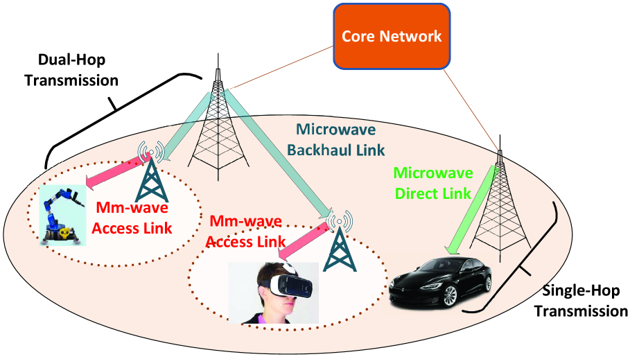
Figure 1: Coexisting sub-6GHz and mm-wave cellular networks.

I-A Related Work

A variety of research works studied the coverage probability of mm-wave only cellular networks [15, 16, 17]. Di Renzo et al. [15] proposed a general mathematical model to analyze multi-tier mm-wave cellular networks. Bai et al. [16] derived the coverage and rate performance of mm-wave cellular networks. They used a distance dependent line-of-sight (LOS) probability function where the locations of the LOS and non-LOS (NLOS) BSs are modeled as two independent non-homogeneous Poisson point processes, to which different path loss models are applied. The authors assume independent Nakagami fading for each link. Different parameters of Nakagami fading are assumed for LOS and NLOS links. Turgut and Gursoy [17] investigated heterogeneous downlink mm-wave cellular networks consisting of $K$ tiers of randomly located BSs where each tier operates in a mm-wave frequency band. They derived coverage probability for the entire network using tools from stochastic geometry. They used Nakagami fading to model small-scale fading. Deng et al. [18] derived the success probability at the typical receiver in mm-wave device-to-device (D2D) networks. The authors considered Nakagami fading and incorporated directional beamforming.

Some recent studies analyzed the coverage or success probability of coexisting $\mu$wave and mm-wave cellular networks. A hybrid cellular network was considered by Singh et al. [19] to estimate the uplink-downlink coverage and rate distribution of self-backhauled mm-wave networks. Elshaer et al. [3] developed an analytical model to characterize decoupled uplink and downlink cell association strategies. The authors showed the superiority of this technique compared to the traditional coupled association in a network with traditional MBSs coexisting with denser mm-wave SBSs. Singh et al. [19] and Elshaer et al. [3] modeled the fading power as Rayleigh fading to enable better tractability.

Compared to traditional coverage analysis conducted in [17, 16, 3], Deng and Haenggi [20] analyzed the meta distribution of the SIR in mm-wave only single-hop D2D networks using the Poisson bipolar model and simplified Rayleigh fading channels for analytical tractability.

I-B Contributions

To the best of our knowledge, our work is the first to characterize the meta distributions of SIR/SNR and data rate for coexisting $\mu$wave and mm-wave networks. Different from previous research in [17, 16, 3, 20], we develop a stochastic geometry framework that takes in consideration (i) coexistence of two different network tiers with completely different channel propagation, interference, and fading models, (ii) dual-hop transmissions enabled by two different spectrums, one in each network tier, and (iii) Nakagami-m fading model with shape parameter $m$ for LOS mm-wave channels. Nakagami-m fading is a generic and versatile distribution that includes Rayleigh distribution (typically used for non-LOS fading) as its special case when $m=1$ and can well approximate the Rician fading distribution for $1\leq m\leq\infty$ (typically used for LOS fading).

We assume a hybrid spectrum network architecture described above and illustrated in Fig. 1. Since microwave transmissions are interference limited and mm-wave transmission are noise limited, we study the meta distributions of the SIR and SNR in $\mu$wave and mm-wave channels, respectively. We also characterize the meta distrubusiton of data rates. Our contributions and methodology include the following:

• Different from existing works, we characterize the CSP (which is equivalent to reliability) of a typical device and its $b^{\mathrm{th}}$ moment when the device either associates to (1) $\mu$wave MBS for direct transmission or (2) mm-wave SBS for dual-hop transmission (access and backhaul transmission). Using the novel moment expressions in the two scenarios, we derive a novel expression for the cumulative moment $M_{b,\text{T}}$ of the considered hybrid spectrum network.

• Using the cumulative moment $M_{b,\text{T}}$, we characterize the exact and approximate meta distributions of the data rate and downlink SIR/SNR of a typical device. Since the expression of $M_{b,\text{T}}$ relies on a Binomial expansion of power $b$, the results for the meta-distribution requiring complex values of $b$ are obtained by applying Newton’s Generalized Binomial Theorem.

• We characterize important network performance metrics such as coverage probability, mean local delay (which is equivalent to latency), and variance of the local delay (network jitter), using the derived cumulative moment $M_{b,\text{T}}$. For metrics with negative values of $b$, we apply the binomial theorem for negative integers.

• To model the LOS nature of mm-wave, we consider the versatile Nakagami-m fading channel model. To the best of our knowledge, the meta distribution for the Nakagami-m fading channel has not been investigated yet.

• We demonstrate the application of this framework to other specialized network scenarios where (i) SBSs are connected to MBSs via a mm-wave wireless backhaul and (ii) a network where all transmissions are conducted in $\mu$wave spectrum. Closed-form results are provided for special cases and asymptotic scenarios.

We validate analytical results using Monte-Carlo simulations. Numerical results give valuable insights related to the reliability, mean local delay, variance of CSP, and standard success probability of a device. For example, the mean local delay increases with the increasing density of SBSs in a $\mu$wave-only network; however, it stays constant in a hybrid spectrum network. Moreover, the data rate reliability, i.e., the fraction of devices achieving a required data rate, increases as the number of antenna elements increases. We also note that as the number of antenna elements in a hybrid spectrum network increases, the reduction in the variance of reliability is noticeable, which shows the importance of analyzing the higher moments of the CSP using the meta distribution. These insights would help 5G cellular network operators to find the most efficient operating antenna configurations for ultra-reliable and low latency applications.

I-C Outline of the Article

The remainder of the article is organized as follows. In Section II, we describe the system model and assumptions. In Section III, we provide mathematical preliminaries of the meta distribution. In Section IV, we characterize the association probabilities of a typical device and formulate the meta distribution of the SIR/SNR of a device in the hybrid spectrum 5G cellular networks. In Section V, we characterize the CSP and its $b^{\mathrm{th}}$ moment for direct, access, and backhaul transmissions. Finally, we derive the exact and approximate meta distributions of the SIR/SNR and data rate in a hybrid spectrum network as well as $\mu$wave-only network in Section VII. Finally, Section VIII presents numerical results and Section IX concludes the article.

II System Model and Assumptions

In this section, we describe the network deployment model (Section II-A), antenna model (Section II-B), channel model (Section II-C), device association criteria (Section II-D), and SNR/SIR models for access and backhaul transmissions (Section II-E).

II-A Network Deployment and Spectrum Allocation Model

We assume a two-tier cellular network architecture as shown in Fig. 1 in which the locations of the MBSs and SBSs are modeled as a two-dimensional (2D) homogeneous Poisson point process (PPP) $\mathbf{\Phi}_{k}=\{\mathbf{y}_{k,1},\mathbf{y}_{k,2},...\}$ of density $\lambda_{k}$, where $\mathbf{y}_{k,i}$ is the location of $i^{\mathrm{th}}$ MBS (when $k=1$) or the $i^{\mathrm{th}}$ SBS (when $k=2$). Let the MBS tier be tier 1 ($k=1$) and the SBSs constitute tier 2 ($k=2$). Let $\mathcal{D}$ denotes the set of devices. The locations of devices in the network are modeled as independent homogeneous PPP $\mathbf{\Phi}_{\mathcal{D}}=\{\mathbf{x}_{1},\mathbf{x}_{2},....\}$ with density $\lambda_{\mathcal{D}}$, where $\mathbf{x}_{i}$ is the location of the $i^{\mathrm{th}}$ device. We assume that $\lambda_{\mathcal{D}}\gg\lambda_{2}>\lambda_{1}$ as in [23, 24, 25]. We consider a typical outdoor device which is located at the origin and is denoted by $0$ and its tagged BS is denoted by $\mathbf{y}_{k,0}$, i.e., tagged MBS (when $k=1$) or tagged SBS (when $k=2$). All BSs in the $k^{\mathrm{th}}$ tier transmit with the same transmit power $P_{k}$ in the downlink. A list of the key mathematical notations is given in Table I.

We assume that a portion $\eta W_{1}$ of the frequency band $W_{1}$ is reserved for the access transmission and the rest $(1-\eta)W_{1}$ is reserved for the backhaul transmission, where $W_{1}$, and $W_{2}$ denote the total available $\mu$wave spectrum and mm-wave spectrum, respectively, and $0\leq\eta\leq 1$. Determining the optimal spectrum allocation ratio $\eta$ will be studied in our future work.

TABLE I: Mathematical Notations

Notation	Description	Notation	Description
$\mathbf{\Phi}_{k}$;$\mathbf{\Phi}_{\mathcal{D}}$	PPP of BSs of $k^{\mathrm{th}}$ tier; PPP of devices	$\lambda_{k}$;$\lambda_{\mathcal{D}}$	Density of BSs of $k^{\mathrm{th}}$ tier; density of devices
$P_{k}$	Transmit power of BSs in $k^{\mathrm{th}}$ tier	$B_{k}$	Association bias for BSs of $k^{\mathrm{th}}$ tier
$\alpha_{1},\alpha_{2,L},\alpha_{2,N}$	Path loss exponent of MBS tier; LOS SBS; NLOS SBS	$G^{o}_{1}$	omnidirectional antenna gain of $\mu$wave MBSs
$G_{2}^{max}$;$G_{2}^{min}$;$\theta_{a}$	Main lobe gain; side lobe gain; and 3 dB beamwidth for mm-wave SBS	$h_{l}$	Gamma fading channel gain for mm-wave SBSs
$g$	Rayleigh fading channel gain	$m_{l}$	Nakagami-m fading parameter where $l\in\{L,N\}$ denotes LOS and NLOS transmission links
$p_{L}$;$p_{N}$	Mm-wave blockage LOS probability; NLOS probability	$\theta$	Predefined SIR/SNR threshold
$\bar{F}_{P_{s}}(x)$	Meta distribution of SIR/SNR	$P_{s}(\theta)$	Conditional success probability (CSP)
$M_{b}(\theta)$	The $b^{th}$ moment of $P_{s}(\theta)$	$\mathcal{A}_{2}$;$\mathcal{A}_{2,L}$;$\mathcal{A}_{2,N}$	Association Probability with $\mu$wave MBS; LOS mm-wave SBS; NLOS mm-wave SBS

II-B Antenna Model

We assume that all MBSs are equipped with omnidirectional antennas with gain denoted by $G^{\mathrm{o}}_{1}$ dB. We consider SBSs and devices are equipped with directional antennas with sectorized gain patterns as in [22, 15, 20] to approximate the actual antenna pattern. The sectorized gain pattern is given by:

$$G_{a}(\theta)=\begin{cases}G_{a}^{\mathrm{max}}&\mbox{if }\left|\theta\right|\leq\frac{\theta_{a}}{2}\\ G_{a}^{\mathrm{min}}&\mbox{otherwise }\end{cases},$$ (1)

where subscript $a\in\{2,\mathcal{D}\}$ denotes for SBSs and devices, respectively. Considering a $\sqrt{\mathcal{N}}\times\sqrt{\mathcal{N}}$ uniform planar square antenna array with $\mathcal{N}$ elements, the antenna parameters of a uniform planar square antenna array can be given as in [20], i.e., $G_{a}^{\mathrm{max}}=\mathcal{N}$ is the main lobe antenna gain, $G_{a}^{\mathrm{min}}=1/\sin^{2}\left(\frac{3\pi}{2\sqrt{\mathcal{N}}}\right)$ is the side lobe antenna gain, $\theta\in[-\pi,\pi)$ is the angle of the boresight direction, and $\theta_{a}=\frac{\sqrt{3}}{\sqrt{\mathcal{N}}}$ is the main lobe beam width. A perfect beam alignment is assumed between a device and its serving SBS [3] [16]. The antenna beams of the desired access links are assumed to be perfectly aligned, i.e., the direction of arrival (DoA) between the transmitter and receiver is known a priori at the BS and the effective gain on the intended access link can thus be denoted as $G_{2}^{\mathrm{max}}G_{\mathcal{D}}^{\mathrm{max}}$. This can be done by assuming that the serving mm-wave SBS and device can adjust their antenna steering orientation using the estimated angles of arrivals. The analysis of the alignment errors on the desired link is beyond the scope of this work.

II-C Channel Model

II-C1 Path-Loss Model

The signal power decay is modeled as $L(r)=r^{\alpha}$, where $L(r)$ is the path loss for a typical receiver located at a distance $r$ from the transmitter and $\alpha$ is the path loss exponent (PLE). Let $L_{1}(r)=\|r_{1,\mathcal{D}}\|^{\alpha_{1}}$ denotes the path loss of a typical device associated with the MBS tier, where $\alpha_{1}$ is the PLE. Similarly, $L_{2}(r)=\|r_{2,\mathcal{D}}\|^{\alpha_{2,l}}$ denotes the path loss of a typical device associated with the SBS tier where $\alpha_{2,l}=\alpha_{2,L}$ is the PLE in the case of LOS and $\alpha_{2,l}=\alpha_{2,N}$ is the PLE in the case of NLOS. It has been shown that mm-wave LOS and NLOS conditions have markedly different PLEs [26]. Also, we consider the near-field path loss factor $\zeta=(\frac{\text{carrier wavelength}}{4\pi})^{2}$ at 1 m [3], i.e., different path loss for different frequencies at the reference distance.

II-C2 Fading Model

For outdoor mm-wave channels, we consider a versatile Nakagami-m fading channel model due to its analytical tractability and following the previous line of research studies [16, 17, 27, 28, 18]. Nakagami-m fading is a general and tractable model to characterize mm-wave channels. Also, in several scenarios, Nakagami-m can approximate the Rician fading which is commonly used to model the LOS transmissions but not tractable for meta distribution modeling [29, 30]. The fading parameter $m_{l}\in[1,2,...,\infty)$ where $l\in\{L,N\}$ denotes LOS and NLOS transmission links, respectively, and the mean fading power is denoted by $\Omega_{l}$. The fading channel power $h_{l}$ follows a gamma distribution given as $f_{h_{l}}(x)=\frac{m_{l}^{m_{l}}x^{m_{l}-1}}{\Omega_{l}^{m_{l}}\Gamma(m_{l})}\exp(\frac{-m_{l}x}{\Omega_{l}})$, $x>0$, where $\Gamma(.)$ is the Gamma function, $m_{l}$ is the shape (or fading) parameter, and $\frac{m_{l}}{\Omega_{l}}$ is the scale parameter. That is, we consider $h_{l}\sim\Gamma(m_{L},1/m_{L})$ for the LOS links and $h_{l}\sim\Gamma(m_{N},1/m_{N})$ for the NLOS links. Rayleigh fading is a special case of Nakagami-m for $m_{L}=m_{N}=1$. Due to the NLOS nature of $\mu$wave channels, we assume Rayleigh fading with power normalization, i.e., the channel gain $g(\mathbf{x},\mathbf{y})\sim\exp(1)$, is independently distributed with the unit mean.

II-C3 Blockage Model for Mm-wave Access Links

For mm-wave channels, LOS transmissions are vulnerable to significant penetration losses [26]; thus LOS transmissions can be blocked with a certain probability. Following [16, 31, 27, 32], we consider the actual LOS region of a device as a fixed LOS ball referred to as ”equivalent LOS ball”. For the sake of mathematical tractability, we consider a distance dependent blockage probability $p(r)$ that a mm-wave link of length $r$ observes, i.e., the LOS probability $p_{L}(r)$ if the mm-wave desired link length is less than $d$ and $p_{N}(r)$ otherwise. That is, SBSs within a LOS ball of radius $d$ are marked LOS with probability $p_{L}(r)$, while the SBSs outside that LOS ball are marked as NLOS with probability $p_{N}(r)$. Note that we will drop the notation $(r)$ in both $p_{L}(r)$ and $p_{N}(r)$ from this point onwards and we will use only $p_{L}$ and $p_{N}$, respectively.

II-D Association Mechanism

Each device associates with either a MBS or a SBS depending on the maximum biased received power in the downlink. The association criterion at the typical device can be written mathematically as follows:

$$P_{k}B_{k}G_{k}\zeta_{k}L_{k}(r)^{-1}\geq P_{j}B_{j}G_{j}\zeta_{j}L_{\mathrm{min},j}(r)^{-1},\forall j\in\{1,2\},j\neq k$$ (2)

where $P_{(\cdot)}$, $B_{(\cdot)}$, $G_{(\cdot)}$, and $\zeta_{(\cdot)}$ denote the transmission power, biasing factor, effective antenna gain, and near-field path loss at 1 m of the intended link, respectively, in the corresponding tier (which is determined by the index in the subscript). Let $L_{\mathrm{min},j}(r)^{-1}$ be the minimum path loss of a typical device from a BS in the $j^{\mathrm{th}}$ tier. When a device associates with a mm-wave SBS in tier-2, i.e., $k=2$, the antenna gain of the intended link is $G_{2}=G_{2}^{\mathrm{max}}G_{\mathcal{D}}^{\mathrm{max}}$, otherwise $G_{1}=G^{\mathrm{o}}_{1}G_{\mathcal{D}}$, where $G^{\mathrm{o}}_{1}$ is defined as the omnidirectional antenna gain of MBSs and $G_{\mathcal{D}}$ is the device antenna gain while operating in $\mu$wave spectrum. On the other hand, the SBS associates with a MBS offering the maximum received power in the downlink.

II-E SNR/SIR Models for Access and Backhaul Transmissions

The device associates to either a MBS for direct transmission or a SBS for dual-hop transmission. The first link (backhaul link) transmissions occur on the $\mu$wave spectrum between MBSs and SBSs and the second link (access link) transmissions take place in the mm-wave spectrum between SBSs and devices. Let $\theta_{2}$ denotes the predefined SIR threshold for SBSs in the backhaul link and $\theta_{\mathcal{D}}$ denotes the predefined SIR/SNR threshold for devices. Throughout the paper, we use subscripts “$1,2$”, “$2,\mathcal{D}$”, “$1,\mathcal{D}$”, “$\mathcal{D}$”, “$\mathrm{BH}$” to denote backhaul link, access link, direct link, device, and backhaul, respectively.

II-E1 Backhaul Transmission

The $\mathrm{SIR}$ of a typical SBS associated with a MBS can be modeled as:

$$\mathrm{SIR}_{1,2}=\frac{P_{1}r_{1,2}^{-\alpha_{1}}g(0,\mathbf{y}_{1,0})}{\mathcal{I}_{1,2}},$$ (3)

where $\mathcal{I}_{1,2}$ denotes the backhaul interference received at a SBS from MBSs that are scheduled to transmit on the same resource block excluding the tagged MBS. Then, $\mathcal{I}_{1,2}=P_{1}\sum_{i:\mathbf{y}_{1,i}\in\mathbf{\Phi}_{1}\backslash\{\mathbf{y}_{1,0}\}}\|\mathbf{y}_{1,i}\|^{-\alpha_{1}}g(0,\mathbf{y}_{1,i}).$

II-E2 Direct Transmission

The $\mathrm{SIR}$ of a typical device associated directly with a MBS is modeled as:

$$\mathrm{SIR}_{1,\mathcal{D}}=\frac{P_{1}r_{1,\mathcal{D}}^{-\alpha_{1}}g(0,\mathbf{y}_{1,0})}{\mathcal{I}_{1,\mathcal{D}}},$$ (4)

where $\mathcal{I}_{1,\mathcal{D}}$ denotes the interference received at a typical device from MBSs excluding the tagged MBS. Then $\mathcal{I}_{1,\mathcal{D}}$ can be calculated as: $\mathcal{I}_{1,\mathcal{D}}=P_{1}\sum_{i:\mathbf{y}_{1,i}\in\mathbf{\Phi}_{1}\backslash\{\mathbf{y}_{1,0}\}}\|\mathbf{y}_{1,i}\|^{-\alpha_{1}}g(0,\mathbf{y}_{1,i}).$

II-E3 Access Transmission

The SNR of a typical device associated with a mm-wave SBS is modeled as:

$$\mathrm{SNR}_{2,\mathcal{D}}=\frac{P_{2}G_{2}\zeta_{2}\|r_{2,\mathcal{D}}\|^{-\alpha_{2,l}}h_{l}(0,\mathbf{y}_{2,0})}{\sigma_{2}^{2}},$$ (5)

where $\zeta_{2}$ is the near-field path loss at 1 m for mm-wave channels, and $\sigma_{2}^{2}$ is the variance of the additive white Gaussian noise at the device receiver. Given highly directional beams and high sensitivity to blockage, recent studies showed that mm-wave networks are typically noise limited [21, 19, 22].

III The Meta Distribution: Mathematical Preliminaries

In this section, we define the meta distribution of the SIR of a typical device and highlight exact and approximate methods to evaluate the meta distribution.

Definition 1 (Meta Distribution of the SIR and CSP).

The meta distribution $\bar{F}_{P_{s}}(x)$ is the complementary cumulative distribution function (CCDF) of the CSP (or reliability) $P_{s}(\theta)$ and given by [9]:

$$\bar{F}_{P_{s}}(x)\overset{\Delta}{=}\mathbb{P}(P_{s}(\theta)>x),\quad\quad x\in[0,1],$$ (6)

where, conditioned on the locations of the transmitters and that the desired transmitter is active, the CSP $P_{s}(\theta)$ of a typical device [9] can be given as $P_{s}(\theta)\overset{\Delta}{=}\mathbb{P}(\mathrm{SIR}>\theta|\mathbf{\Phi},\text{tx})$ where $\theta$ is the desired $\mathrm{SIR}$.

Physically, the meta distribution provides the fraction of the active links whose CSP (or reliability) is greater than the reliability threshold $x$. Given $M_{b}(\theta)$ denotes the $b^{\mathrm{th}}$ moment of $P_{s}(\theta)$, i.e., $M_{b}(\theta)\overset{\Delta}{=}\mathbb{E}^{0}(P_{s}(\theta)^{b})$, $b\in\mathbb{C}$, the exact meta distribution can be given using the Gil-Pelaez theorem [33] as [9]:

$$\bar{F}_{P_{s}}(x)=\frac{1}{2}+\frac{1}{\pi}\int_{0}^{\infty}\frac{\Im\left(e^{-jt\log{x}}M_{jt}(\theta)\right)}{t}\text{d}t,$$ (7)

where $\Im(w)$ is imaginary part of $w\in\mathbb{C}$ and $M_{jt}(\theta)$ denotes the imaginary moments of $P_{s}(\theta)$, i.e., , $j\overset{\Delta}{=}\sqrt{-1}$. Using moment matching techniques and taking $\beta\overset{\Delta}{=}\frac{(M_{1}(\theta)-M_{2}(\theta))(1-M_{1}(\theta))}{M_{2}(\theta)-M_{1}(\theta)^{2}}$, the meta distribution of the CSP can be approximated using the Beta distribution as follows:

$$\bar{F}_{P_{s}}(x)\approx 1-I_{x}\left(\frac{\beta M_{1}(\theta)}{1-M_{1}(\theta)},\beta\right),\quad\quad x\in[0,1],$$ (8)

where $M_{1}(\theta)$ and $M_{2}(\theta)$ are the first and the second moments, respectively; $I_{x}(a,b)$ is the regularized incomplete Beta function $I_{x}(a,b)\overset{\Delta}{=}\frac{\int_{0}^{x}t^{a-1}(1-t)^{b-1}d\text{t}}{B(a,b)}$ and $B(a,b)$ is the Beta function.

IV The Meta Distribution of the SIR/SNR in Hybrid Spectrum Networks

To characterize the meta distribution of the SIR/SNR of a typical device that can associate with either a $\mu$wave MBS with probability $\mathcal{A}_{1}$ or with a wireless backhauled mm-wave SBS with probability $\mathcal{A}_{2}$, the methodology of analysis is listed as follows:

1. Derive the probability of a typical device associating with $\mu$wave MBSs $\mathcal{A}_{1}$, LOS mm-wave SBSs $\mathcal{A}_{2,{\rm L}}$, and NLOS mm-wave SBSs $\mathcal{A}_{2,{\rm N}}$ where $\mathcal{A}_{2}=\mathcal{A}_{2,{\rm L}}+\mathcal{A}_{2,{\rm N}}$ (Section IV-A).

2. Formulate the meta distribution of the SIR/SNR of a device in the hybrid network ($\bar{F}^{b}_{P_{s,\text{T}}}(x)$) considering the direct link and dual-hop link with wireless backhaul transmission (Section IV-B).

3. Formulate the CSP (${P_{s,\text{T}}}(\theta)$) and its $b^{\mathrm{th}}$ moment $(M_{b,\text{T}})$ (Section IV-B).

4. Derive the CSP at backhaul link $P_{s,\mathrm{BH}}(\theta_{2})$, CSP at access link $P_{s,2}(\theta_{\mathcal{D}})$, and CSP at direct link $P_{s,1}(\theta_{\mathcal{D}})$. Derive the $b^{\mathrm{th}}$ moments of CSPs, i.e., $M_{b,\mathrm{BH}}(\theta_{2})$, $M_{b,2}(\theta_{\mathcal{D}})$, and $M_{b,1}(\theta_{\mathcal{D}})$ for backhaul link, access link, and direct link transmissions, respectively (Section V).

5. Obtain the meta distributions of SIR/SNR and data rate in hybrid spectrum network using Gil-Pelaez inversion and the Beta approximation (Section VI).

IV-A Association Probabilities in Hybrid Spectrum Networks

In this subsection, we characterize the probabilities with which a typical device associates with $\mu$wave MBSs ($\mathcal{A}_{1}$) or mm-wave SBSs ($\mathcal{A}_{2}$). The results are presented in the following.

Lemma 1 (The Probability of Associating with mm-wave SBSs).

The probability of a typical device to associate with a mm-wave SBS, using the association scheme in Eq. (2), can be expressed as:

$$\mathcal{A}_{2}=1-\frac{2\pi\lambda_{1}}{\hat{a}\alpha_{1}}\Bigg{(}\int_{0}^{d^{\alpha_{2,L}}}H(l_{1})e^{-\pi\lambda_{2}p_{L}l_{1}^{\frac{2}{\alpha_{2,L}}}}d\text{l}_{1}+\int_{d^{\alpha_{2,L}}}^{d^{\alpha_{2,N}}}H(l_{1})e^{-\pi\lambda_{2}p_{L}d^{2}}d\text{l}_{1}+\int_{d^{\alpha_{2,N}}}^{\infty}H(l_{1})e^{-\pi\lambda_{2}\bigg{[}(p_{L}-p_{N})d^{2}+p_{N}l_{1}^{\frac{2}{\alpha_{2,N}}}\bigg{]}}d\text{l}_{1}\Bigg{)},$$ (9)

where $\hat{a}\overset{\Delta}{=}\frac{P_{2}B_{2}G_{2}\zeta_{2}}{P_{1}B_{1}G_{1}\zeta_{1}}$ and $H(l_{1})\overset{\Delta}{=}\left(\frac{l_{1}}{\hat{a}}\right)^{\frac{2}{\alpha_{1}}-1}\exp\left(-\pi\lambda_{1}\left(\frac{l_{1}}{\hat{a}}\right)^{\frac{2}{\alpha_{1}}}\right)$. Subsequently, the probability of a device to associate with a $\mu$wave MBS can be given as $\mathcal{A}_{1}=1-\mathcal{A}_{2}$. The conditional association probability for a typical device to associate with SBS is as follows:

$$\bar{\mathcal{A}}_{2}(l_{1}) =1-\frac{2\pi\lambda_{1}}{\hat{a}\alpha_{1}}\Bigg{(}H(l_{1})e^{-\pi\lambda_{2}p_{L}l_{1}^{\frac{2}{\alpha_{2,L}}}}+H(l_{1})e^{-\pi\lambda_{2}p_{L}d^{2}}+H(l_{1})e^{-\pi\lambda_{2}\left[(p_{L}-p_{N})d^{2}+p_{N}l_{1}^{\frac{2}{\alpha_{2,N}}}\right]}\Bigg{)},$$ (10)

subsequently, $\bar{\mathcal{A}}_{1}(l_{1})=1-\bar{\mathcal{A}}_{2}(l_{1})$.

Proof.

Using the approach in [3], we derive Lemma 1 in Appendix A of our technical report [34]. ∎

A closed-form expression of $\mathcal{A}_{1}$ can be derived for a case of practical interest as follows.

Corollary 1.

When $\alpha_{1}=4$, $\alpha_{2,L}=2$, and $\alpha_{2,N}=4$, then $\mathcal{A}_{1}$ can be given in closed-form as follows:

$$\mathcal{A}_{1}=\frac{e^{C}(\Phi[\sqrt{C}+\sqrt{\pi\lambda_{2}p_{L}d^{2}}]-\Phi[\sqrt{C}])}{\sqrt{p_{L}\lambda_{2}/\hat{a}}}+\frac{e^{-d^{2}\pi p_{L}\lambda_{2}}(e^{-\pi\lambda_{1}\sqrt{d^{2}/\hat{a}}}-e^{-\pi\lambda_{1}\sqrt{d^{4}/\hat{a}}})}{\pi\lambda_{1}/2\hat{a}}+\frac{e^{d^{2}\pi(p_{N}-p_{L})\lambda_{2}-C_{1}\sqrt{d^{4}/\hat{a}}})}{C_{1}/2\hat{a}},$$ (11)

where $\Phi(\cdot)$ is the error function, $C=\frac{\pi\lambda^{2}_{1}}{4\hat{a}p_{L}\lambda_{2}}$ and $C_{1}=\pi(\lambda_{1}+\sqrt{\hat{a}}p_{N}\lambda_{2})$ and $\mathcal{A}_{2}=1-\mathcal{A}_{1}$.

It can be seen from Corollary 1 that when the number of antenna elements $\mathcal{N}$ goes to infinity, i.e., $G_{2}\rightarrow\infty$, $\hat{a}\rightarrow\infty$, then $\mathcal{A}_{1}$ can be simplified as $\mathcal{A}_{1}=\frac{\Phi[\sqrt{\pi\lambda_{2}p_{L}d^{2}}]}{\sqrt{p_{L}\lambda_{2}/\hat{a}}}+\frac{e^{d^{2}\pi(p_{N}-p_{L})\lambda_{2}}}{C_{1}/2\hat{a}},$ which shows that association probability to MBS will be very small. Similar insights can be extracted for other parameters.

In order to derive the $b^{\mathrm{th}}$ moment of CSP $P_{s,2}(\theta_{\mathcal{D}})$ on an access link when a device associates with a SBS (the CSP will be discussed later in Lemma 4), we have to derive the probability of a device to associate with LOS SBS $\mathcal{A}_{2,L}$ and NLOS SBS $\mathcal{A}_{2,N}$ which are defined follows.

Lemma 2 (The Probability of Associating with LOS and NLOS mm-wave SBSs).

When a typical device associates with the mm-wave SBS tier, this typical device has two possibilities to connect to (a) a LOS mm-wave SBS with association probability $\mathcal{A}_{2,L}$ and (b) a NLOS mm-wave SBS with association probability $\mathcal{A}_{2,N}$ which are characterized, respectively, as follows:

$$\mathcal{A}_{2,L} =\int_{0}^{d^{\alpha_{2,L}}}\bar{\mathcal{A}}_{2,L}(l_{2,L})d\text{l}_{2,L},\quad\mathcal{A}_{2,N}=\int_{d^{\alpha_{2,N}}}^{\infty}\bar{\mathcal{A}}_{2,N}(l_{2,N})d\text{l}_{2,N},$$ (12)

where $\bar{\mathcal{A}}_{2,L}(l_{2,L})$ and $\bar{\mathcal{A}}_{2,N}(l_{2,N})$ are the conditional probabilities with which a typical device may associate to the LOS and NLOS mm-wave SBSs, respectively, and are defined as follows:

$$\bar{\mathcal{A}}_{2,L}(l_{2,L})\overset{\Delta}{=} \frac{2\pi\lambda_{2}p_{L}}{\alpha_{2,L}}l_{2,L}^{\frac{2}{\alpha_{2,L}}-1}e^{\left(-\pi\lambda_{1}\left(\bar{a}l_{2,L}\right)^{\frac{2}{\alpha_{1}}}-\pi\lambda_{2}p_{L}l_{2,L}^{\frac{2}{\alpha_{2,L}}}\right)},$$

$$\bar{\mathcal{A}}_{2,N}(l_{2,N})\overset{\Delta}{=} \frac{2\pi\lambda_{2}p_{N}}{\alpha_{2,N}}l_{\text{2,N}}^{\frac{2}{\alpha_{2,N}}-1}\exp\left(-\pi\lambda_{1}\left(\bar{a}l_{2,N}\right)^{\frac{2}{\alpha_{1}}}-\pi\lambda_{2}\big{[}p_{L}d^{2}+p_{N}(l_{2,N}^{\frac{2}{\alpha_{2,N}}}-d^{2})\big{]}\right)d\text{l}_{2,N},$$

where $\bar{a}\overset{\Delta}{=}\frac{P_{1}B_{1}G_{1}\zeta_{1}}{P_{2}B_{2}G_{2}\zeta_{2}}$, $\bar{\mathcal{A}}_{2}(l_{2})=\bar{\mathcal{A}}_{2,L}(l_{2,N})+\bar{\mathcal{A}}_{2,N}(l_{2,N})$ and $\mathcal{A}_{2}=\mathcal{A}_{2,L}+\mathcal{A}_{2,N}$.

Proof.

Using the approach in [17], we derive Lemma 2 in Appendix B of our technical report [34]. ∎

A case of interest is when the number of antenna elements at mm-wave SBSs increases asymptotically. In such a case, the LOS and NLOS association probabilities can be simplified as follows:

Corollary 2.

When the number of antenna elements at mm-wave SBSs increases, i.e., $\mathcal{N}\rightarrow\infty$, $\alpha_{1}=4$, $\alpha_{2,L}=2$, and $\alpha_{2,N}=4$, then $\bar{a}\rightarrow 0$. The association probabilities can be given in closed-form as follows: $\mathcal{A}_{2,L}{=}1-e^{-\pi p_{L}d^{2}\lambda_{2}}$, $\quad\quad\mathcal{A}_{2,N}{=}e^{d^{2}\pi(-p_{L}+p_{N})\lambda_{2}}(1-\pi p_{N}d^{2}\lambda_{2}\>{}_{1}F_{1}[1;2;\pi p_{N}d^{2}\lambda_{2}]),$

where $\>{}_{1}F_{1}[a;b;z]$ is the Kummer Confluent Hypergeometric function.

An interesting insight from Corollary 2 can be seen when the intensity of SBSs $\lambda_{2}\rightarrow\infty$ or $d$ is large, the probability of association to LOS SBSs $\mathcal{A}_{2,L}$ becomes almost 1. On the other hand, when $\lambda_{2}\rightarrow 0$ or $d$ is small, $\>{}_{1}F_{1}[a;b;0]=1$ thus $\mathcal{A}_{2,N}$ becomes almost 1.

IV-B Formulation of the Meta distribution, CSP and its $b^{\mathrm{th}}$ Moment in the Hybrid Network

When a device associates with a mm-wave SBS, the overall CSP depends on the CSPs of the SIR and SNR on both the backhaul link and the access link, respectively. On the other hand, when a device associates to MBS the CSP depends on the SIR of the direct link. It is thus necessary to formulate the relationship between the meta distribution, CSP, and its $b^{\mathrm{th}}$ moment in the considered hybrid network as follows.

Lemma 3 (Meta Distribution of the Typical device in the Hybrid Network).

The combined meta distribution of the SIR/SNR in the hybrid spectrum network can be characterized as follows:

$$\bar{F}_{P_{s,\text{T}}}(x)=\frac{1}{2}+\frac{1}{\pi}\int_{0}^{\infty}\frac{\Im\left(e^{-jt\log{x}}M_{jt,\text{T}}(\cdot)\right)}{t}\text{d}t,$$ (13)

where $M_{jt,\text{T}}(\theta)$ can be characterized by deriving the $b^{\mathrm{th}}$ moment of the $P_{s,\text{T}}(\cdot)$.

$$M_{b,\text{T}}(\cdot) ={M_{b,\mathrm{Dual-Hop}}}+{M_{b,\mathrm{Single-Hop}}}\stackrel{{\scriptstyle(a)}}{{=}}\mathbb{E}_{\Phi}[\bar{\mathcal{A}}_{2}(l_{2})P^{b}_{s,\mathrm{Dual-Hop}}(\theta_{2})]+\mathbb{E}_{\Phi}[\bar{\mathcal{A}}_{1}(l_{1})P^{b}_{s,1}(\theta_{\mathcal{D}})],$$

$$\stackrel{{\scriptstyle(b)}}{{=}}\mathbb{E}_{\Phi}\bigg{[}\bar{\mathcal{A}}_{2}(l_{2})(P_{s,\mathrm{BH}}(\theta_{2})P_{s,2}(\theta_{\mathcal{D}}))^{b}\bigg{]}+\mathbb{E}_{{\Phi}}\bigg{[}\bar{\mathcal{A}}_{1}(l_{1})P^{b}_{s,1}(\theta_{\mathcal{D}})\bigg{]},$$

$$\stackrel{{\scriptstyle(c)}}{{=}}\mathbb{E}_{{\Phi}}\bigg{[}P_{s,\mathrm{BH}}(\theta_{2})^{b}\bigg{]}\mathbb{E}_{{\Phi}}\bigg{[}\bar{\mathcal{A}}_{2}(l_{2})P_{s,2}(\theta_{\mathcal{D}})^{b}\bigg{]}+\mathbb{E}_{\Phi}\bigg{[}\bar{\mathcal{A}}_{1}(l_{1})P^{b}_{s,1}(\theta_{\mathcal{D}})\bigg{]},$$

$$\stackrel{{\scriptstyle(d)}}{{=}}\mathbb{E}_{{\Phi}}\bigg{[}P_{s,\mathrm{BH}}(\theta_{2})^{b}\bigg{]}\mathbb{E}_{{\Phi}}\bigg{[}(\bar{\mathcal{A}}_{2,L}(l_{2,L})+\bar{\mathcal{A}}_{2,N}(l_{2,N}))P_{s,2}(\theta_{\mathcal{D}})^{b}\bigg{]}+\mathbb{E}_{\Phi}\bigg{[}\bar{\mathcal{A}}_{1}(l_{1})P^{b}_{s,1}(\theta_{\mathcal{D}})\bigg{]},$$

$$\stackrel{{\scriptstyle(e)}}{{=}}\underbrace{M_{b,\mathrm{BH}}(\theta_{2})M_{b,2}(\theta_{\mathcal{D}})}_{\text{Device Associated with SBS}}+\underbrace{M_{b,1}(\theta_{\mathcal{D}})}_{\text{Device Associated with MBS}},$$ (14)

where ${M_{b,\mathrm{Dual-Hop}}}$ is the $b^{\mathrm{th}}$ moment of the SIR/SNR when a device associates to mm-wave SBS for dual-hop transmission and $M_{b,\mathrm{Single-Hop}}$ is the $b^{\mathrm{th}}$ moment of the SIR when a device associates to MBS for direct transmission. After reformulation, we define $M_{b,\mathrm{BH}}(\theta_{2})$ as the unconditional $b^{\mathrm{th}}$ moment of the backhaul SIR, $M_{b,2}(\theta_{\mathcal{D}})$ as the unconditional $b^{\mathrm{th}}$ moment of the SNR at access link when a device associates to mm-wave SBS, and $M_{b,1}(\theta_{\mathcal{D}})$ as the unconditional $b^{\mathrm{th}}$ moment of the SIR at direct link when a device associates to $\mu$wave BS. Note that $P_{s,1}(\theta_{\mathcal{D}})\overset{\Delta}{=}\mathbb{P}(\mathrm{SIR_{1,\mathcal{D}}}>\theta_{\mathcal{D}}|\mathbf{\Phi}_{1},\text{tx})$ denotes the CSP of device over the direct link, $P_{s,\mathrm{BH}}(\theta_{2})\overset{\Delta}{=}\mathbb{P}(\mathrm{SIR_{1,2}}>\theta_{2}|\mathbf{\Phi_{1}},\text{tx})$ denotes the CSP at backhaul link, and $P_{s,2}(\theta_{\mathcal{D}})\overset{\Delta}{=}\mathbb{P}(\mathrm{SNR_{2,\mathcal{D}}}>\theta_{\mathcal{D}}|\mathbf{\Phi}_{2},\text{tx})$ denotes the CSP for the access link transmission.

Proof.

Step (a) follows from the fact that the $b^{\mathrm{th}}$ moment of the SIR or SNR of a device associated to tier $i$ can be defined as $M_{b}^{(i)}=\mathbb{E}[\bar{\mathcal{A}_{i}}M_{b|i}]$ where $\bar{\mathcal{A}_{i}}$ is the conditional association probability to tier $i$ and $M_{b|i}=P^{b}_{s,i}$ is the conditional $b^{\mathrm{th}}$ moment of the SIR or SNR in tier $i$. In our case, we have $\bar{\mathcal{A}}_{2}(l_{2})$ which is the conditional association probability to mm-wave SBS where $l_{2}\in\{L,N\}$ since a device can associate to either LOS or NLOS mm-wave SBS. The step (b) follows from the fact that the CSP of the dual-hop transmission depends on the CSP of access and backhaul link; therefore, we have a product of the access and backhaul CSPs, i.e., $P_{s,\mathrm{BH}}(\theta_{2})P_{s,2}(\theta_{\mathcal{D}})$ that are independent random variables. There is no correlation since $\mu$wave backhaul does not interfere with mm-wave transmissions. The step (c) follows from the fact if $X$ and $Y$ are independent then $\mathbb{E}[(XY)^{b}]=\mathbb{E}[X^{b}]\mathbb{E}[Y^{b}]$. Finally, the step (d) follows from the definition of $\bar{\mathcal{A}}_{2}(l_{2})$ in Lemma 2 and the step (e) follows by applying the definition of moments. ∎

In the next section, we derive the CSP of access, backhaul, and direct links along with their respective $b^{\mathrm{th}}$ moments, as needed in Lemma 4 to characterize the overall moment as well as the meta distribution.

V Characterization of the CSPs and Moments

In this section, we derive the CSPs $P_{s,\mathrm{BH}}(\theta_{2}),P_{s,2}(\theta_{\mathcal{D}}),P_{s,1}(\theta_{\mathcal{D}})$ and the $b^{\mathrm{th}}$ moments $M_{b,\mathrm{BH}}(\theta_{2})$, $M_{b,2}(\theta_{\mathcal{D}})$, and $M_{b,1}(\theta_{\mathcal{D}})$ for backhaul link, access link, and direct link, respectively.

V-A CSP and the $b^{\mathrm{th}}$ Moment - Access Link

We condition on having a device at the origin which becomes a typical device. The CSP of a typical device at the origin associating with the mm-wave SBS-tier (when $k=2$) can be described as follows:

$$P_{s,2}(\theta_{\mathcal{D}})=p_{L}P_{s,2,L}(\theta_{\mathcal{D}})+p_{N}P_{s,2,N}(\theta_{\mathcal{D}}).$$ (15)

The CSP of the SNR of a device on the access link with LOS can be defined by substituting $\mathrm{SNR}_{2,\mathcal{D}}$ defined in Eq. (5) into Definition 1 as follows:

$$P_{s,2,L}(\theta_{\mathcal{D}}) =\mathbb{P}\left(h_{L}(0,\mathbf{y}_{2,0})>\frac{\theta_{\mathcal{D}}r_{2,\mathcal{D}}^{\alpha_{2,L}}\sigma_{2}^{2}}{P_{2}G_{2}}|\mathbf{\Phi}_{1},\mathbf{\Phi}_{2},\text{tx}\right)\stackrel{{\scriptstyle(a)}}{{=}}1-\frac{\gamma\left(m_{L},\frac{m_{L}}{\Omega_{L}}\nu_{L}\right)}{\Gamma{(m_{L})}}\stackrel{{\scriptstyle(b)}}{{=}}\frac{\Gamma\left(m_{L},\frac{m_{L}}{\Omega_{L}}\nu_{L}\right)}{\Gamma{(m_{L})}},$$ (16)

where (a) follows from the definition of $\nu_{L}\overset{\Delta}{=}\frac{\theta_{\mathcal{D}}r_{2,\mathcal{D}}^{\alpha_{2,L}}\sigma_{2}^{2}}{P_{2}G_{2}}$ and the fact that the channel gain $h_{L}(0,\mathbf{y}_{2,0})$ is a normalized gamma random variable and $\gamma(.,.)$ is the lower incomplete gamma function and $\Gamma(s)=\gamma(s,x)+\Gamma(s,x)$, where $\Gamma(.,.)$ is the upper incomplete gamma function. Similarly, CSP of the SNR on the access link for NLOS case can be given as follows:

$$P_{s,2,N}(\theta_{\mathcal{D}}) =\frac{\Gamma\left(m_{N},\frac{m_{N}}{\Omega_{N}}\nu_{N}\right)}{\Gamma(m_{N})},$$ (17)

where $\nu_{N}\overset{\Delta}{=}\frac{\theta_{\mathcal{D}}r_{2,\mathcal{D}}^{\alpha_{2,N}}\sigma_{2}^{2}}{P_{2}G_{2}}$. As such, the $\boldsymbol{b^{th}}$ moment of the CSP on the access link for the typical device when it is served by the mm-wave SBS tier is given by the following:

Lemma 4.

The $b^{\mathrm{th}}$ moment of the SNR at an “access link” when a device associates with a mm-wave SBS can be characterized as follows:

$$M_{b,\text{2}}(\theta_{\mathcal{D}})=$$

$$\sum_{k=0}^{b}\binom{b}{k}(-1)^{k}\left(p_{L}^{b}\sum_{\ddot{k}=0}^{m_{L}k}\binom{m_{L}k}{\ddot{k}}(-1)^{\ddot{k}}\int_{0}^{d^{\alpha_{2,L}}}e^{-\zeta_{L}\ddot{k}\ddot{\nu_{L}}l_{\text{2,L}}}\bar{\mathcal{A}}_{2,L}(l_{2,L})+p_{N}^{b}\sum_{\ddot{k}=0}^{m_{N}k}\binom{m_{N}k}{\ddot{k}}(-1)^{\ddot{k}}\int_{d^{\alpha_{2,N}}}^{\infty}e^{-\zeta_{N}\ddot{k}\ddot{\nu_{N}}l_{\text{2,N}}}\bar{\mathcal{A}}_{2,N}(l_{2,N})\right),$$ (18)

where $\bar{\mathcal{A}}_{2,L}(l_{2,L})$ and $\bar{\mathcal{A}}_{2,N}(l_{2,N})$ are given in Lemma 2, $\zeta_{L}\overset{\Delta}{=}m_{L}(m_{L}!)^{-1/m_{L}}$, $\nu_{L}\overset{\Delta}{=}\frac{\theta_{\mathcal{D}}r_{2,\mathcal{D}}^{\alpha_{2,L}}\sigma_{2}^{2}}{P_{2}G_{2}}$, $\zeta_{N}\overset{\Delta}{=}m_{N}(m_{N}!)^{-1/m_{N}}$, and $\nu_{N}\overset{\Delta}{=}\frac{\theta_{\mathcal{D}}r_{2,\mathcal{D}}^{\alpha_{2,N}}\sigma_{2}^{2}}{P_{2}G_{2}}$, $\ddot{\nu_{L}}\overset{\Delta}{=}\frac{\nu_{L}}{r^{\alpha_{2,L}}}=\frac{\nu_{L}}{l_{\text{2,L}}}=\frac{\theta_{\mathcal{D}}\sigma_{2}^{2}}{P_{2}G_{2}}$ and $\ddot{\nu_{N}}\overset{\Delta}{=}\frac{\nu_{N}}{r^{\alpha_{2,N}}}=\frac{\nu_{N}}{l_{\text{2,N}}}=\frac{\theta_{\mathcal{D}}\sigma_{2}^{2}}{P_{2}G_{2}}$.

Proof.

See Appendix C. ∎

For $\alpha_{1}=4$, $\alpha_{2,L}=2$, and $\alpha_{2,N}=4$, we can get $M_{b,\text{2}}(\theta_{\mathcal{D}})$ in closed-form using Corollary 1. Also, for scenarios where $\mathcal{N}\rightarrow\infty$, $\alpha_{1}=4$, $\alpha_{2,L}=2$, and $\alpha_{2,N}=4$, then $\bar{a}\rightarrow 0$. Also, $\ddot{v}_{L}\rightarrow 0$ and $\ddot{v}_{N}\rightarrow 0$, we can get $M_{b,\text{2}}(\theta_{\mathcal{D}})$ in closed-form using Corollary 2.

V-B CSP and Moment - Backhaul Link

For the backhaul link, we condition on having a SBS at the origin which becomes the typical SBS. Using the expression of $\mathrm{SIR}_{1,2}$ in Eq. (3) the CSP of the backhaul link $P_{s,\mathrm{BH}}(\theta_{2})$ can be given as:

$$P_{s,\mathrm{BH}}(\theta_{2}) =\mathbb{P}\left(g(0,\mathbf{y}_{1,0})>\frac{\theta_{2}r_{1,2}^{\alpha_{1}}}{P_{1}}\mathcal{I}_{1,2}|\mathbf{\Phi}_{1},\mathbf{\Phi}_{2},\text{tx}\right)\stackrel{{\scriptstyle(a)}}{{=}}\mathbb{E}\bigg{[}\exp(-\theta_{2}r_{1,2}^{\alpha_{1}}\sum_{i:\mathbf{y}_{1,i}\in\mathbf{\Phi}_{1}\backslash\{\mathbf{y}_{1,0}\}}\|\mathbf{y}_{1,i}\|^{-\alpha_{1}}g(0,\mathbf{y}_{1,i}))\bigg{]},$$

$$=\prod_{\mathbf{y}_{1,i}\in\mathbf{\Phi}_{1}\backslash\{\mathbf{y}_{1,0}\}}\mathbb{E}\bigg{[}\exp\left(-\theta_{2}r_{1,2}^{\alpha_{1}}\|\mathbf{y}_{1,i}\|^{-\alpha_{1}}g(0,\mathbf{y}_{1,i})\right)\bigg{]}\stackrel{{\scriptstyle(b)}}{{=}}\prod_{\mathbf{y}_{1,i}\in\mathbf{\Phi}_{1}\backslash\{\mathbf{y}_{1,0}\}}\frac{1}{1+\theta_{2}\left(\frac{r_{1,2}}{\|\mathbf{y}_{1,i}\|}\right)^{\alpha_{1}}}.$$ (19)

where (a) follows from the Rayleigh fading channel gain $g(0,\mathbf{y}_{1,0})\sim\exp(1)$ and (b) is found by taking the expectation with respect to $g(0,\mathbf{y}_{2,i})$. The $\boldsymbol{b^{th}}$ moment of the CSP on the backhaul link is given as:

$$M_{b,\mathrm{BH}}(\theta_{2}) =\mathbb{E}\bigg{[}P_{s,\mathrm{BH}}(\theta_{2})^{b}\bigg{]}=\mathbb{E}\bigg{[}\prod_{\mathbf{y}_{1,i}\in\mathbf{\Phi}_{1}\backslash\{\mathbf{y}_{1,0}\}}\frac{1}{\left(1+\theta_{2}\left(\frac{r_{1,2}}{\|\mathbf{y}_{1,i}\|}\right)^{\alpha_{1}}\right)^{b}}\bigg{]},$$

$$\stackrel{{\scriptstyle(a)}}{{=}}\left({1+2\int_{0}^{1}\left(1-\frac{1}{(1+\theta_{2}r^{\alpha_{1}})^{b}}\right)r^{-3}dr}\right)^{-1}{=}\frac{1}{\text{ }_{2}F_{1}(b,-\frac{2}{\alpha_{1}};1-\frac{2}{\alpha_{1}};-\theta_{2})},$$ (20)

where (a) follows from the probability generating functional (PGFL) of PPP, i.e., $G_{\mathcal{R}}[f]\overset{\Delta}{=}\mathbb{E}\prod_{x\in\mathcal{R}}f(x)=\frac{1}{1+2\int_{0}^{1}(1-f(x))x^{-3}dx}.$ [35, lemma 1] and ${\text{}_{2}F_{1}(.,.;.;.)}$ represents Gauss‘ Hyper-geometric function.

V-C CSP and Moment - Direct Link

Using the expression of $\mathrm{SIR}_{1,\mathcal{D}}$ in Eq. (4), we calculate the CSP of the direct link $P_{s,1}(\theta_{\mathcal{D}})$ as follows:

$$P_{s,1}(\theta_{\mathcal{D}}) =\mathbb{P}\left(g(0,\mathbf{y}_{1,0})>\frac{\theta_{\mathcal{D}}r_{1,\mathcal{D}}^{\alpha_{1}}}{P_{1}}\mathcal{I}_{1,\mathcal{D}}|\mathbf{\Phi}_{1},\mathbf{\Phi}_{2},\text{tx}\right)\stackrel{{\scriptstyle(a)}}{{=}}\mathbb{E}\bigg{[}\exp\left(-\theta_{\mathcal{D}}r_{1,\mathcal{D}}^{\alpha_{1}}\sum_{i:\mathbf{y}_{1,i}\in\mathbf{\Phi}_{1}\backslash\{\mathbf{y}_{1,0}\}}\|\mathbf{y}_{1,i}\|^{-\alpha_{1}}g(0,\mathbf{y}_{1,i})\right)\bigg{]},$$

$$=\prod_{\mathbf{y}_{1,i}\in\mathbf{\Phi}_{1}\backslash\{\mathbf{y}_{1,0}\}}\mathbb{E}\bigg{[}\exp\left(-\theta_{\mathcal{D}}r_{1,\mathcal{D}}^{\alpha_{1}}\|\mathbf{y}_{1,i}\|^{-\alpha_{1}}g(0,\mathbf{y}_{1,i})\right)\bigg{]}\stackrel{{\scriptstyle(b)}}{{=}}\prod_{\mathbf{y}_{1,i}\in\mathbf{\Phi}_{1}\backslash\{\mathbf{y}_{1,0}\}}\frac{1}{1+\theta_{\mathcal{D}}\left(\frac{r_{1,\mathcal{D}}}{\|\mathbf{y}_{1,i}\|}\right)^{\alpha_{1}}},$$ (21)

where (a) follows from the channel gain $g(0,\mathbf{y}_{1,0})\sim\exp(1)$ and is independently exponentially distributed with unit mean and (b) is obtained by taking the expectation with respect to $g(0,\mathbf{y}_{1,i})$. While taking the association probabilities into consideration, the $\boldsymbol{b^{th}}$ moment of the CSP $P_{s,1}(\theta_{\mathcal{D}})$ of the typical device when it is served by a $\mu$wave MBS is characterized in the following lemma.

Lemma 5 (The $b^{\mathrm{th}}$ moment of the CSP ($P_{s,1}(\theta_{\mathcal{D}})$) when a device associates with a MBS).

The $b^{\mathrm{th}}$ moment of the CSP experienced by a device, when the device associates with a MBS, can be characterized as follows:

$$M_{b,\text{1}}(\theta_{\mathcal{D}})=\frac{2\pi\lambda_{1}}{\hat{a}\alpha_{1}}\Bigg{\{}\int_{0}^{d^{\alpha_{2,L}}}H(l_{1})\exp\left(-\pi\lambda_{2}p_{L}l_{1}^{\frac{2}{\alpha_{2,L}}}\right)d\text{l}_{1}+\int_{d^{\alpha_{2,L}}}^{d^{\alpha_{2,N}}}H(l_{1})\exp\left(-\pi\lambda_{2}p_{L}d^{2}\right)d\text{l}_{1}+$$

$$\quad\quad\quad\quad\int_{d^{\alpha_{2,N}}}^{\infty}H(l_{1})\exp\left(-\pi\lambda_{2}[p_{L}d^{2}+p_{N}\left(l_{1}^{\frac{2}{\alpha_{2,N}}}-d^{2}\right)\right)d\text{l}_{1}\Bigg{\}}\times\exp\left(\frac{-2\lambda_{1}\pi l_{1}^{\frac{2}{\alpha_{1}}}}{\alpha_{1}}\int_{0}^{1}\bigg{[}1-\frac{1}{\left(1+\theta_{\mathcal{D}}v\right)^{b}}\bigg{]}\frac{1}{v^{\frac{2}{\alpha_{1}}+1}}\text{d}v\right),$$ (22)

Proof.

See Appendix D. ∎

Note that $\int_{0}^{1}\bigg{[}1-\frac{1}{\left(1+\theta_{\mathcal{D}}v\right)^{b}}\bigg{]}\frac{1}{v^{\frac{2}{\alpha_{1}}+1}}\text{d}v$ is independent of $l_{1}$, thus where $\mathcal{N}\rightarrow\infty$ or $\alpha_{1}=4$, $\alpha_{2,L}=2$, and $\alpha_{2,N}=4$, then we can get a closed-form for the three integral over $l_{1}$ using Corollary 1 and Corollary 2.

V-D Combined $b^{\mathrm{th}}$ Moment of the CSP in Hybrid Networks

After substituting the values of $M_{b,\mathrm{BH}}(\theta_{2})$, $M_{b,2}(\theta_{\mathcal{D}})$, and $M_{b,1}(\theta_{\mathcal{D}})$ in Eq. (V-B), Eq. (4), and Eq. (5), respectively into the total meta distribution for the entire network in Eq. (3), we get the $b^{\mathrm{th}}$ moment of the CSP at a typical device as follows:

$$M_{b,\text{T}}=\frac{1}{\text{ }_{2}F_{1}(b,-\frac{2}{\alpha_{1}};1-\frac{2}{\alpha_{1}};-\theta_{2})}\times\bigg{\{}\sum_{k=0}^{b}\binom{b}{k}(-1)^{k}\left(p_{L}^{b}\sum_{\ddot{k}=0}^{m_{L}k}\binom{m_{L}k}{\ddot{k}}(-1)^{\ddot{k}}\int_{0}^{d^{\alpha_{2,L}}}e^{-\zeta_{L}\ddot{k}\ddot{\nu_{L}}l_{\text{2,L}}}\bar{\mathcal{A}}_{2,L}(l_{2,L})+\right.$$

$$\quad\quad\quad\quad\quad\quad\quad\quad\quad\quad\quad\quad\quad\quad\quad\quad\left.p_{N}^{b}\sum_{\ddot{k}=0}^{m_{N}k}\binom{m_{N}k}{\ddot{k}}(-1)^{\ddot{k}}\int_{d^{\alpha_{2,N}}}^{\infty}e^{-\zeta_{N}\ddot{k}\ddot{\nu_{N}}l_{\text{2,N}}}\bar{\mathcal{A}}_{2,N}(l_{2,N})\right)\bigg{\}}+M_{b,1}(\theta_{\mathcal{D}}),$$ (23)

In the next section, we use the combined $b^{\mathrm{th}}$ moment in (V-D) to compute the meta distributions of SIR/SNR and data rate using Gil-Pelaez inversion and the Beta approximation.

VI Computing the Meta Distributions and Special Cases

In this section, we compute the meta distribution of SIR/SNR using Gil-Pelaez inversion and beta approximation by applying the derived result of $M_{b,\text{T}}$. Special cases where $b=1$ provides the standard coverage probability and $b=-1$ provides the mean local delay are discussed. Further, we show how to evaluate the data rate meta distribution from the derived framework.

VI-A Computing the Meta Distribution of SIR/SNR

Technically, substituting $b=jt$ in (V-D), we should obtain the imaginary moments $M_{jt,\text{T}}$. However, since the expression of $M_{jt,\text{T}}$ relies on a Binomial expansion of power $b$, the results cannot be obtained directly through substitution. Therefore, we apply Newton’s generalized binomial theorem given as follows:

Definition 2.

Isaac Newton‘s generalized binomial theorem is to allow real exponents other than non-negative integers, i.e., imaginary exponent $r$, as $\binom{r}{k}=\frac{r(r-1)...(r-k+1)}{k!}=\frac{(r)_{k}}{k!},$ where $(.)_{k}$ is the Pochhammer symbol, which stands here for a falling factorial.

Applying Definition 2 in step (e) of Appendix C, we then obtain the expression for $M_{jt,\text{T}}$ as follows:

$$M_{jt,\text{T}}=\frac{1}{\text{ }_{2}F_{1}(jt,-\frac{2}{\alpha_{1}};1-\frac{2}{\alpha_{1}};-\theta_{2})}\times\bigg{\{}p_{L}^{jt}\sum_{k=0}^{\infty}\frac{(jt)_{k}}{k!}(-1)^{k}\sum_{\ddot{k}=0}^{m_{L}k}\binom{m_{L}k}{\ddot{k}}(-1)^{\ddot{k}}\int_{0}^{d^{\alpha_{2,L}}}e^{-\zeta_{L}\ddot{k}\ddot{\nu_{L}}l_{\text{2,L}}}\bar{\mathcal{A}}_{2,L}(l_{2,L})+$$

$$\quad\quad\quad\quad\quad\quad\quad\quad\quad\quad p_{N}^{jt}\sum_{k=0}^{\infty}\frac{(jt)_{k}}{k!}(-1)^{k}\sum_{\ddot{k}=0}^{m_{N}k}\binom{m_{N}k}{\ddot{k}}(-1)^{\ddot{k}}\int_{d^{\alpha_{2,N}}}^{\infty}e^{-\zeta_{N}\ddot{k}\ddot{\nu_{N}}l_{\text{2,N}}}\bar{\mathcal{A}}_{2,N}(l_{2,N})\bigg{\}}+M_{jt,1}(\theta_{\mathcal{D}}),$$ (24)

The imaginary moments can be substituted in the Gil-Pelaez inversion theorem as in Definition 1 to obtain $\bar{F}_{P_{s},\text{T}}$. Furthermore, we follow [9, 13, 36] to approximate the meta distribution by a Beta distribution by matching the first and second moments, which are easily obtained from the general result in Eq. (V-D) by substituting $b=1$ and $b=2$ to get $M_{1,\text{T}}$ and $M_{2,\text{T}}$, respectively. Taking $\beta\overset{\Delta}{=}\frac{(M_{1,\text{T}}-M_{2,\text{T}})(1-M_{1,\text{T}})}{M_{2,\text{T}}-M_{1,\text{T}}^{2}}$, the meta distribution using beta approximation can be given as follows:

$$\bar{F}_{P_{s,\text{T}}}(x)\approx 1-I_{x}\left(\frac{\beta M_{1,\text{T}}}{1-M_{1,\text{T}}},\beta\right),\quad\quad x\in[0,1],$$ (25)

VI-B Mean and Variance of the Local Delay

The mean local delay is the mean number of transmission attempts, i.e., re-transmissions, needed to successfully transmit a packet to the target receiver. The mean local delay $M_{-1,\text{T}}$ which is the $-1^{\mathrm{st}}$ moment of the CSP of a typical device should be calculated by substituting $b=-1$ in Eq. (V-D). However, since the expression of $M_{b,\text{T}}$ relies on a Binomial expansion of power $b$, the results cannot be obtained directly through substitution. Therefore, we apply Binomial theorem for the negative integers as follows:

Definition 3.

The Binomial theorem for a negative integer power $n$ can be given [37] as $(x+y)^{n}=\sum_{k=0}^{\infty}(-1)^{k}\binom{-n+k-1}{k}y^{n-k}x^{k},$

Applying Definition 3 in step (e) of Appendix C, we then obtain the expression for $M_{-1,\text{T}}$ as follows:

$$M_{-1,\text{T}}=\frac{1}{\text{ }_{2}F_{1}(-1,-\frac{2}{\alpha_{1}};1-\frac{2}{\alpha_{1}};-\theta_{2})}\times\bigg{\{}p_{L}^{-1}\sum_{k=0}^{\infty}\sum_{\ddot{k}=0}^{m_{L}k}\binom{m_{L}k}{\ddot{k}}(-1)^{\ddot{k}}\int_{0}^{d^{\alpha_{2,L}}}e^{-\zeta_{L}\ddot{k}\ddot{\nu_{L}}l_{\text{2,L}}}\bar{\mathcal{A}}_{2,L}(l_{2,L})+$$

$$\quad\quad\quad\quad\quad\quad\quad\quad\quad\quad\quad\quad\quad\quad\quad p_{N}^{-1}\sum_{k=0}^{\infty}\sum_{\ddot{k}=0}^{m_{N}k}\binom{m_{N}k}{\ddot{k}}(-1)^{\ddot{k}}\int_{d^{\alpha_{2,N}}}^{\infty}e^{-\zeta_{N}\ddot{k}\ddot{\nu_{N}}l_{\text{2,N}}}\bar{\mathcal{A}}_{2,N}(l_{2,N})dl_{2,N}\bigg{\}}+M_{-1,1}(\theta_{\mathcal{D}}),$$ (26)

Remark: In order to better characterize the fluctuation of the local delay, the variance of the local delay also referred to as network jitter can be given by $NJ=M_{-2,\text{T}}-M_{-1,\text{T}}^{2}.$

VI-C The Meta Distribution of the Data Rate in Hybrid Spectrum Networks

Let $\mathcal{T}$ denote the data rate (in bits/sec) of the typical device on a specific transmission link which is a random variable and is defined as $\mathcal{R}=W\log_{2}(1+\mathrm{SIR})$ using Shannon capacity. Using the meta distribution of the SIR, the meta distribution of the data rate can be derived to present the fraction of active devices in each realization of the point process that have a data rate $\mathcal{R}$ greater than $\mathcal{T}$ with probability at least $x$, i.e., devices data rate reliability threshold. That is, first deriving the CSP of the data rate as follows:

$$\mathbb{P}[\mathcal{R}>\mathcal{T}|\mathbf{\Phi},\text{tx}] =\mathbb{P}[W\log_{2}(1+\mathrm{SIR})>\mathcal{T}|\mathbf{\Phi},\text{tx}]=\mathbb{P}[\mathrm{SIR}>2^{\frac{\mathcal{T}}{W}}-1|\mathbf{\Phi},\text{tx}],$$ (27)

where $P_{s}(2^{\frac{\mathcal{T}}{W}}-1)\overset{\Delta}{=}\mathbb{P}(\mathrm{SIR}>2^{\frac{\mathcal{T}}{W}}-1|\mathbf{\Phi}_{1},\text{tx})$ denote the CSP of the device data rate over single link. Finally, deriving the $b^{\mathrm{th}}$ moment of the CSP of the data rate and applying Gil-Pelaez inversion we can obtain the meta distribution of the data rate.

Corollary 3.

Similar to the meta distribution of the SIR/SNR derived in Lemma 3 and conditioned on the location of the point process, we derive the meta distribution of the data rate in hybrid 5G cellular networks, using the moment $\mathcal{Q}_{b}$ of the conditional data rate as follows:

$$\mathcal{Q}_{b}(\mathcal{T})=\mathbb{E}[\bar{\mathcal{A}}_{2}(l_{2})\mathbb{P}^{0}\left(P_{s,\mathrm{BH}}(2^{\frac{\mathcal{T}_{\mathrm{BH}}}{(1-\eta)W_{1}}}-1)P_{s,2}(2^{\frac{\mathcal{T}_{2}}{W_{2}}}-1)>x\right)]+\mathbb{E}[\bar{\mathcal{A}}_{1}(l_{1})\mathbb{P}^{0}(P_{s,1}(2^{\frac{\mathcal{T}_{1}}{\eta W_{1}}}-1)>x)],$$

$$=M_{b,\mathrm{BH}}\left(2^{\frac{\mathcal{T}_{\mathrm{BH}}}{(1-\eta)W_{1}}}-1\right)M_{b,2}\left(2^{\frac{\mathcal{T}_{2}}{W_{2}}}-1\right)+M_{b,1}\left(2^{\frac{\mathcal{T}_{1}}{\eta W_{1}}}-1\right),$$ (28)

where $P_{s,1}(2^{\frac{\mathcal{T}_{1}}{\eta W_{1}}}-1)\overset{\Delta}{=}\mathbb{P}(\mathrm{SIR_{1,\mathcal{D}}}>2^{\frac{\mathcal{T}_{1}}{\eta W_{1}}}-1|\mathbf{\Phi}_{1},\text{tx})$, $P_{s,\mathrm{BH}}(2^{\frac{\mathcal{T}_{\mathrm{BH}}}{(1-\eta)W_{1}}}-1)\overset{\Delta}{=}\mathbb{P}(\mathrm{SIR_{1,2}}>2^{\frac{\mathcal{T}_{\mathrm{BH}}}{(1-\eta)W_{1}}}-1|\mathbf{\Phi_{1}},\text{tx})$, and $P_{s,2}(2^{\frac{\mathcal{T}_{2}}{W_{2}}}-1)\overset{\Delta}{=}\mathbb{P}(\mathrm{SNR_{2,\mathcal{D}}}>2^{\frac{\mathcal{T}_{2}}{W_{2}}}-1|\mathbf{\Phi}_{2},\text{tx})$ denotes the CSP of the device data rate at the direct, backhaul, and access link, respectively.

In the following section, we discuss the application of this framework in two scenarios (i) $\mu$wave only network and (ii) mm-wave backhauls and microwave access links.

VII Extensions of The Model to Other Network Architectures

The framework discussed above can be flexibly applied to different network architectures. In this section we discuss how to extend the framework to two other network architectures: 1) both tiers operating in the sub-6GHz (microwave) spectrum as in traditional cellular networks; and 2) the two tiers operating in two millimeter-wave spectrums which are orthogonal to each other. Due to space limitation, we provide only general directions of how to extend the earlier framework to these two other network architectures.

VII-A The Meta Distribution of the SIR in Microwave-only Cellular Networks

We characterize the meta distribution of the downlink $\mathrm{SIR}$ attained at a typical device in a $\mu$wave-only cellular network, i.e., the access and backhaul links of SBSs operate in the $\mu$wave frequency. A device associates with either a serving MBS for direct transmissions (when $k=1$) or a SBS for dual-hop transmissions (when $k=2$), depending on the biased received signal power criterion. MBSs and SBSs are assumed to operate on orthogonal spectrums; thus, there is no inter-tier interference. On the other hand, each SBS associates with a MBS based on the maximum received power at the SBS. The association criterion for a typical device can be described as follows [38]:

$$P_{k}B_{k}(\min_{i}\|\mathbf{y}_{k,i}-\mathbf{x}\|)^{-\alpha_{k}}\geq P_{j}B_{j}(\min_{i^{{}^{\prime}}}\|\mathbf{y}_{j,i^{{}^{\prime}}}-\mathbf{x}\|)^{{-\alpha_{j}}},\forall j$$ (29)

where $\|.\|$ denotes the Euclidean distance. A typical device associates with a serving node (given by Eq. (29))), which is termed the tagged SBS. For the sake of clarity, we define $\hat{P}_{jk}\overset{\Delta}{=}\frac{P_{j}}{P_{k}}$, $\hat{B}_{jk}\overset{\Delta}{=}\frac{B_{j}}{B_{k}}$, $\hat{\lambda}_{jk}\overset{\Delta}{=}\frac{\lambda_{j}}{\lambda_{k}}$. As derived in [38], the conditional association probability for the typical device connecting to the $k^{\mathrm{th}}$ tier (conditional over the desired link distance $r_{\mathcal{D},k}$) is as follows:

$$\mathbb{P}(n=k|r_{\mathcal{D},k})=\prod_{j\neq k}e^{-\pi\lambda_{j}(\hat{P}_{jk}\hat{B}_{jk})^{2/\alpha_{j}}r^{2}},$$ (30)

where $n$ denotes the index of the tier associating with the typical device. We calculate the CSP $P_{s,2^{\prime}}(\theta_{\mathcal{D}})$ (when $k=2$) of the access link operating in the $\mu$wave band as follows:

$$P_{s,2^{\prime}}(\theta_{\mathcal{D}})=\mathbb{P}\left(g(0,\mathbf{y}_{2,0})>\frac{\theta_{\mathcal{D}}r_{2,\mathcal{D}}^{\alpha_{2}}}{P_{2}}\mathcal{I}_{2,\mathcal{D}}|\mathbf{\Phi}_{1},\mathbf{\Phi}_{2},\text{tx}\right),$$

$$\stackrel{{\scriptstyle(a)}}{{=}}\mathbb{E}\bigg{[}\exp\left(-\theta_{\mathcal{D}}r_{2,\mathcal{D}}^{\alpha_{2}}\sum_{i:\mathbf{y}_{2,i}\in\mathbf{\Phi}_{2}\backslash\{\mathbf{y}_{2,0}\}}\|\mathbf{y}_{2,i}\|^{-\alpha_{2}}g(0,\mathbf{y}_{2,i})\right)\bigg{]}\stackrel{{\scriptstyle(b)}}{{=}}\prod_{\mathbf{y}_{2,i}\in\mathbf{\Phi}_{2}\backslash\{\mathbf{y}_{2,0}\}}\frac{1}{1+\theta_{\mathcal{D}}\left(\frac{r_{2,\mathcal{D}}}{\|\mathbf{y}_{2,i}\|}\right)^{\alpha_{2}}}.$$ (31)

where (a) follows from the channel gain $g(0,\mathbf{y}_{2,0})\sim\exp(1)$ and is independently exponentially distributed with unit mean and (b) is obtained by taking the expectation with respect to $g(0,\mathbf{y}_{2,i})$.

Lemma 6.

Using Eq. (V-C) and Eq. (VII-A), we calculate a general expression for the $\boldsymbol{b^{\mathrm{th}}}$ moment of the CSP on direct link $M_{b,\text{k'}}$ (when $k=2$) and the $\boldsymbol{b^{th}}$ moment of the CSP at access link (when $k=1$) as:

$$M_{b,\text{k'}} =\frac{1}{\sum\limits_{j\neq k}\hat{\lambda}_{jk}(\hat{P}_{jk}\hat{B}_{jk})^{2/\alpha_{j}}+\text{ }_{2}F_{1}(b,-\frac{2}{\alpha_{k}};1-\frac{2}{\alpha_{k}};-\theta_{\mathcal{D}})}.$$ (32)

Proof.

See Appendix E. ∎

Note that Lemma 6 is novel and different from [39] where we derive the $b^{\mathrm{th}}$ moment of CSP for orthogonal spectrum two tier network while the work in [39] is done for shared spectrum tiers.

Similarly, the moment of the CSP of a typical device with offloading biases is defined as follows:

$$M_{b,\text{T}} =\underbrace{M_{b,\text{dual-hop}}}_{\text{Dual-hop transmission}}+\underbrace{M_{b,1^{\prime}}(\theta_{\mathcal{D}})}_{\text{Direct transmission}}\stackrel{{\scriptstyle(a)}}{{=}}M_{b,\mathrm{BH}}(\theta_{2})M_{b,2^{\prime}}(\theta_{\mathcal{D}})+M_{b,1^{\prime}}(\theta_{\mathcal{D}}),$$ (33)

where $M_{b,\mathrm{BH}}(\theta_{2})$, $M_{b,2^{\prime}}(\theta_{\mathcal{D}})$, and $M_{b,1^{\prime}}(\theta_{\mathcal{D}})$ are defined in Eq. (V-B), Eq. (32) (when $k=2$), and Eq. (32) (when $k=1$), respectively. The step (a) follows from the similar approach as taken in Lemma 4.

$$M_{b,\text{dual-hop}} =\mathbb{E}\bigg{[}P_{s,\mathrm{BH}}(\theta_{2})^{b}\times\prod_{j\neq k}e^{-\pi\lambda_{j}(\hat{P}_{jk}\hat{B}_{jk})^{2/\alpha_{j}}r^{2}}P_{s,2^{\prime}}(\theta_{\mathcal{D}})^{b}\bigg{]},$$

$$\stackrel{{\scriptstyle(a)}}{{=}}\underbrace{\mathbb{E}\bigg{[}P_{s,\mathrm{BH}}(\theta_{2})^{b}\bigg{]}}_{\text{$M_{b,\mathrm{BH}}(\theta_{2})$(Backhaul link )}}\underbrace{\mathbb{E}\bigg{[}\prod_{j\neq k}e^{-\pi\lambda_{j}(\hat{P}_{jk}\hat{B}_{jk})^{2/\alpha_{j}}r^{2}}P_{s,2^{\prime}}(\theta_{\mathcal{D}})^{b}\bigg{]}}_{\text{$M_{b,2}(\theta_{\mathcal{D}})$(access link)}},$$

$$\stackrel{{\scriptstyle(b)}}{{=}}\frac{1}{\text{ }_{2}F_{1}(b,-\frac{2}{\alpha_{1}};1-\frac{2}{\alpha_{1}};-\theta_{2})}\times\frac{1}{\hat{\lambda}_{12}(\hat{P}_{12}\hat{B}_{12})^{2/\alpha_{1}}+\text{ }_{2}F_{1}(b,-\frac{2}{\alpha_{2}};1-\frac{2}{\alpha_{2}};-\theta_{\mathcal{D}})},$$ (34)

where (a) follows from the independence between the location of the MBSs and SBSs. In step (b) we substitute $M_{b,\text{BH}}(\theta_{2})$ from Eq. (V-B) and $M_{b,\text{2'}}(\theta_{\mathcal{D}})$ into Eq. (32) when $k=2$. By substituting Eq. (VII-A) and Eq. (32) (when $k=1$) in Eq. (33), we get the $b^{\mathrm{th}}$ moment $M_{b,\text{T}}$. Finally, by substituting $M_{b,\text{T}}$ in Eq. (33) into either Eq. (13) or Eq. (8), we get the meta distribution of the $\mathrm{SIR}$.

VII-B Extensions to Millimeter-wave Backhauls Networks

The proposed framework can be extended to a scenario where the backhaul and access transmissions are conducted on orthogonal mm-wave spectrums. Note that Eq. (3) will be changed similar to Eq. (5). Then, only the first term, $M_{b,\mathrm{BH}}(\theta_{2})$ in the main Eq. (3) of our model that characterizes the moment of the CSP in the backhaul will be re-defined as $M_{b,\mathrm{BH}}(\theta_{2})=\mathbb{E}[P^{b}_{s,2}(\theta_{2})]$.

The framework can also be extended to a scenario where the backhaul transmissions are conducted on the mm-wave spectrum and the access links of SBSs operate on $\mu$-wave. In this case, we will need to use the results in Section VII.A while redefining the term $M_{b,\mathrm{BH}}(\theta_{2})$ as $M_{b,\mathrm{BH}}(\theta_{2})=\mathbb{E}[P^{b}_{s,2}(\theta_{2})]$ in (VII-A).

VIII Numerical Results and Discussions

We present the simulation parameters in Section VIII-A. Then, we validate our numerical results using Monte-Carlo simulations in Section VIII-B. In Section VIII-B, we use the developed analytical models to obtain insights related to the meta distribution of the SIR/SNR of a typical device, mean and variance of the success probability, transmission delay, and the reliability of a typical device in the downlink direction.

VIII-A Simulation Parameters

Unless otherwise stated, we use the following simulation parameters throughout our numerical results. The transmission powers of MBSs and SBSs in the downlink are $P_{1}=50$ Watts and $P_{2}=5$ Watts, respectively. The size of the simulated network is $90\text{km}\times 90\text{km}$. We assume that the density of MBSs is $\lambda_{1}=2$ MBSs/km² and the density of SBSs is $\lambda_{2}=70$ SBSs/km². The offloading biases for the MBSs and the SBSs are $B_{1}=B_{2}=1$, respectively. The PLE for MBSs is set to $\alpha_{1}=4$ and for mm-wave SBSs, $\alpha_{2,L}=2$ in the case of LOS and $\alpha_{2,N}=4$ in the case of NLOS. The network downlink bandwidth is 100 MHz for $\mu$wave MBSs and 1 GHz for mm-wave SBSs with channel frequency 28 GHz. The LOS (NLOS) states are modeled by large (small) values of $m$, i.e., $m_{L}=2$ and $m_{N}=1$ [17]. SBSs number of antenna elements is $\mathcal{N}=10$. The receiver noise is calculated as [19] $\sigma_{2}^{2}=-174\text{ dBm/Hz}+10\log_{10}(W_{2})+10\text{ dB}$, where $W_{2}=1\text{ GHz}$ is bandwidth allocated to the mm-wave SBSs. The antenna gains of MBSs are $G^{\mathrm{o}}_{1}=0$ dB and devices directional antenna gain is $G^{\mathrm{max}}_{\mathcal{D}}=10$ dB.

VIII-B Numerical Results and Discussions

VIII-B1 Association Probability

Fig. 3 illustrates the accuracy of association probabilities in a hybrid spectrum network, derived in Lemma 1 and Lemma 2, as a function of $\lambda_{2}$ by showing a comparison with Monte-Carlo simulations. We notice from Fig. 3 that by increasing the density of the mm-wave SBSs $\lambda_{2}$, the probability of association with mm-wave LOS SBSs $\mathcal{A}_{2,L}$ increases which confirms the insights from Corollary 1 and Corollary 2. The reason is the increasing number of SBSs per unit area within the LOS ball will favour the device association towards LOS SBSs and reduces the chances of associating with NLOS SBSs. The addition of $\mathcal{A}_{1}+\mathcal{A}_{2,L}+\mathcal{A}_{2,N}=1$ is equal to unity for different densities of SBSs $\lambda_{2}$. Note that the probability of associating with $\mu$wave MBSs is minimal due to a higher path-loss exponent and NLOS omnidirectional transmissions from MBSs.

VIII-B2 The Meta Distribution of the SIR/SNR

In Fig. 3, we validate our analytical results for the meta distribution of the SIR/SNR of a typical device in a hybrid spectrum network through simulations. Fig. 3 also depicts the probability of achieving reliability $x$, i.e., $x\%$ fraction of devices can achieve their quality of service for $\theta\in\{10,1,0.1\}$ dB. From Fig. 3, we note that about 18% of the devices (when $\theta=10$), 51% of devices (when $\theta=1$), and 96% of devices (when $\theta=0.1$) have success probabilities equal to $0.3$.

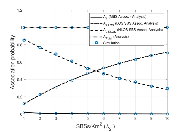
Figure 2: Association probabilities as a function of $\lambda_{2}$ for the hybrid spectrum network when $\lambda_{1}=2\text{ MBSs/km}^{2}$, $B_{1}=B_{2}=1$, and $d=200\text{m}$.

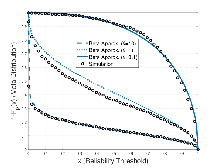
Figure 3: The meta distribution vs. reliability threshold $x$ for $\theta=\theta_{\mathcal{D}}=\theta_{2}=$10, 1, and 0.1 for the hybrid spectrum network when $B_{1}=B_{2}=1$, and $d=200\text{m}$.

VIII-B3 Coverage and Variance as a Function of SIR/SNR Threshold in Hybrid Spectrum Networks

Fig. 5 illustrates the standard success probability $M_{1,\text{T}}$ and its variance $M_{2,\text{T}}-M^{2}_{1,\text{T}}$ as a function of target SIR/SNR threshold $\theta$ of devices in a hybrid spectrum network. As we can see in Fig. 5 that the simulation results match the analytical results, however the slight gap is due to the Alzer’s inequality considered in Appendix C. This gap will be zero when Nakagami fading turns into Rayleigh fading as shown in the next figure. By examining Fig. 5, a numerical evaluation shows that the variance is maximized at $\theta=-3$ dB where the success is $M_{1,\text{T}}=0.49$. For moderate values of $\theta$, there is a trade-off between maximizing coverage or reducing variance because the variance first increases and then decreases while the coverage probability is monotonically decreasing. For higher values of $\theta$, lower coverage probabilities have lower variance so its a low-reliability regime where more devices’ performances are spread around low coverage probability. As such, the low values of $\theta$ provides a higher reliability regime.

Fig. 5 illustrates the standard success probability $M_{1,\text{T}}$ and the variance as a function of $\theta$ with Rayleigh fading (i.e., $m_{L}=m_{N}=1$). As we can see in Fig. 5 that the simulation results closely match the analytical results. The reason is that the approximation of the incomplete Gamma function (also referred to as Alzer’s inequality) becomes exact when $m_{L}$ becomes equal to unity. Subsequently, this figure explains the reason for the gap between the simulation and the analytical curves in Fig. 5.

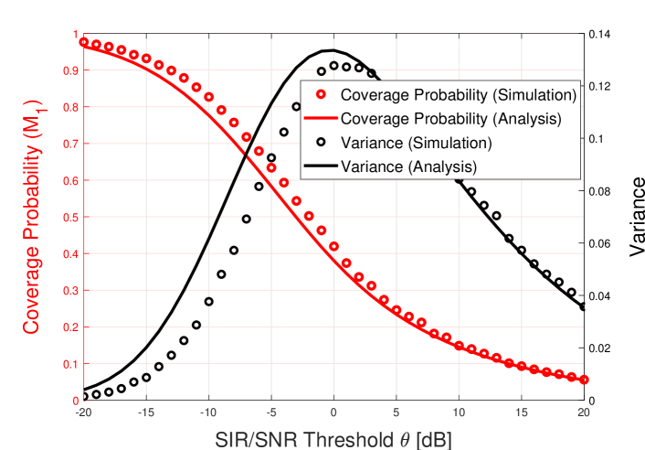
Figure 4: Coverage probability $M_{1,\text{T}}$ and variance $M_{2,\text{T}}-M_{1,\text{T}}^{2}$ as a function of $\theta$ considering Nakagami-m fading when $B_{1}=B_{2}=1$ and $d=200\text{m}$.

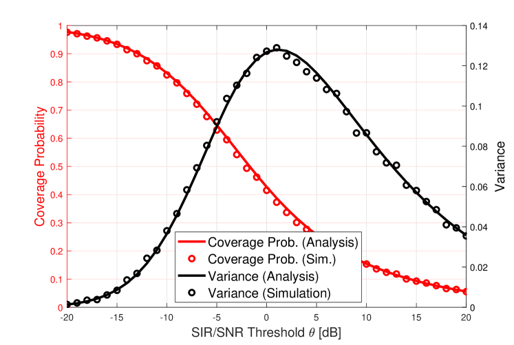
Figure 5: Coverage probability $M_{1,\text{T}}$ and variance $M_{2,\text{T}}-M_{1,\text{T}}^{2}$ as a function of $\theta$ considering Rayleigh fading (i.e., $m_{L}=m_{N}=1$, when $B_{1}=B_{2}=1$ and $d=200\text{m}$.

VIII-B4 Coverage and Variance as a Function of the Number of Antenna Array Elements in Hybrid Spectrum Networks

Fig. 7 depicts the coverage probability and variance as a function of $\theta$ considering the number of antenna array elements as $\mathcal{N}=10$, 20, and 30 to show the effect of higher directional antenna gains. The general trends for the coverage probability and its variance are found to be the same as in previous figures. The main observation is that although the coverage enhancement is not significant with increasing antenna elements, the reduction in the variance is noticeable which supports higher directional antenna gains and the importance of analyzing the higher moments of the CSP.

VIII-B5 Coverage and Variance as a Function of $B_{2}$ in $\mu$wave-only Networks

In Fig. 7, we study the effect of offloading devices from the MBS tier to the SBSs tier in terms of the coverage probability (which is the mean reliability) and the variance of the CSP (or reliability). By offloading devices from the MBS tier to the SBSs tier when $B_{2}=30$, the coverage probability $M_{1,\text{T}}$ suffers due to the dual-hop transmission effect in wireless backhauled SBSs; however the variance of the results reduces which is a novel and positive insight. Another observation is that the variance of the CSP in $\mu$wave-only network is high compared to the hybrid network. This can be shown by comparing points $V_{1}=(1,0.1)$ in Fig. 7 and $V_{2}=(4,0.19)$ in Fig. 7, for the case of $B_{1}=B_{2}=1$. We noticed that the variance has decreased from 0.19 to 0.1 when the SBS antenna array size is increased to $\mathcal{N}=20$. This implies that the hybrid spectrum network outperforms the $\mu$wave-only network due to the directional antenna gains.

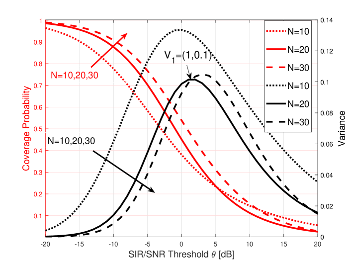
Figure 6: Coverage probability $M_{1,\text{T}}$ and variance $M_{2,\text{T}}-M_{1,\text{T}}^{2}$ as a function of $\mathcal{N}$ for hybrid spectrum network when $B_{1}=B_{2}=1$, and $d=200\text{m}$.

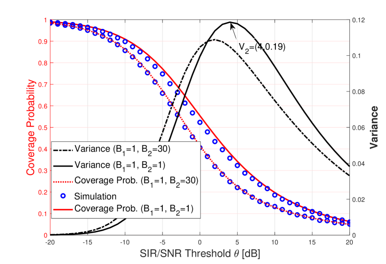
Figure 7: Coverage probability $M_{1,\text{T}}$ and variance $M_{2,\text{T}}-M_{1,\text{T}}^{2}$ as a function of $\theta$ for $\mu$wave-only network when $\alpha_{1}=\alpha_{2}=4$, $B_{1}=1$, and $B_{2}=1$ and 30.

VIII-B6 Mean Local Delay ($\mu$wave vs mm-wave SBSs)

Fig. 9 depicts the mean local delay experienced by a typical device as a function of the SBSs density $\lambda_{2}$ in a hybrid spectrum network. The mean local delay is the mean number of transmission attempts to successfully transmit a packet. The mean local delay increases by increasing $\lambda_{2}$. After the SBS density reaches $\lambda_{2}=20\text{ SBSs/km}^{2}$, the mean local delay stays constant at value 1.11. This result can be intuitively explained as follows. When the mm-wave SBS density is low, the typical device has a higher probability to connect to a MBS, i.e., the mean local delay of the network results from only one hop communication (from the MBS to the device). However, when the $\lambda_{2}$ increases, the typical device has a higher probability to connect to a mm-wave SBS, i.e., the network local delay results from two hops communication (from the MBS to the SBS then from the SBS to the device). Furthermore, the beamforming high directional gain steerable antennas will push more devices to associate with SBSs thus a higher network delay is observed. Fig. 9 shows that, all else being equal, the mean local delay of the hybrid spectrum network is lower than that of the $\mu$wave-only network.

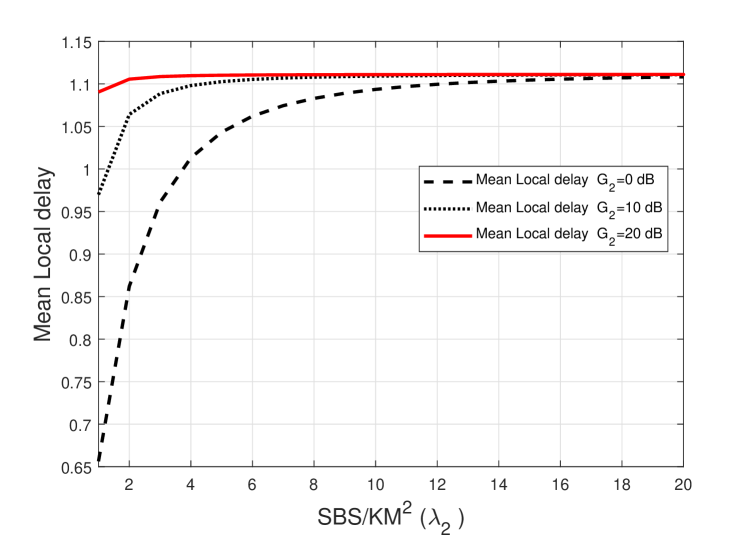
Figure 8: Mean local delay $M_{-1,\text{T}}$ as a function of $\lambda_{2}$ for the hybrid spectrum network when $\lambda_{1}=2\text{ MBS/Km}^{2}$, $B_{1}=1$, $B_{2}=10$, $\alpha_{1}=4$, $d=200\text{m}$, and $\theta=\theta_{\mathcal{D}}=\theta_{2}=$-10 dB.

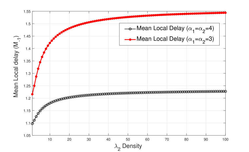
Figure 9: Mean local delay $M_{-1,\text{T}}$ as a function of $\lambda_{2}$ for the $\mu$wave-only network when $\lambda_{1}=2\text{ MBS/KM}^{2}$, $B_{1}=1$ and $B_{2}=10$, $\alpha_{1}=\alpha_{2}=3$ and 4, and $\theta=\theta_{\mathcal{D}}=\theta_{2}=$-10 dB.

Fig. 9 depicts the mean local delay for a $\mu$wave-only network as a function of $\lambda_{2}$. When $\lambda_{2}$ increases the mean local delay of the total network increases again due to the increase in interference which is not the case in the hybrid spectrum network. The network mean local delay in the case of $\alpha_{1}=\alpha_{2}=3$ is higher than that in the case of $\alpha_{1}=\alpha_{2}=4$ due to higher path loss degradation for higher PLEs.

VIII-B7 The Meta Distribution of the Achievable Data Rate in Hybrid Spectrum Networks

Fig. 11 depicts the meta distribution of the data rate in hybrid spectrum networks as a function of reliability $x$ for different number of antenna elements $\mathcal{N}=10$, 20, 40, and 50 with rate threshold $\mathcal{T}=1$ Gbps. As shown in Fig. 11, the fraction of devices achieving a required rate increases as the number of antennas elements increases. In other words, increasing the number of antenna elements of SBSs has a positive effect on the achievable rate and its meta distribution. This insight helps 5G cellular network operators to find the most efficient operating antenna configuration to achieve certain reliability for certain 5G applications.

VIII-B8 The Meta Distribution in a Microwave-only Network

In Fig. 11, we validate our analysis by depicting the exact (Gil-Pelaez) meta distribution in a $\mu$wave-only network defined in Eq. (13), and the beta approximation for the meta distribution defined in Eq. (8). Our simulation result provides an excellent match for a wide range of $\theta$ values and this validates the correctness of our analytical model. Fig. 11 also serves as an illustration of the meta distribution of the SIR of a typical device in a $\mu$wave-only network. We note that about 23% of devices (when $\theta=10$), 72% of devices (when $\theta=1$), and 98% of devices (when $\theta=0.1$) have reliability, i.e., success probability, equal to $0.3$.

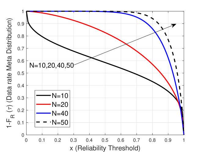
Figure 10: Meta distribution of the achievable data rate as a function of reliability $x$ for different number of antenna elements $\mathcal{N}$ with rate threshold $\mathcal{T}=1$ Gbps.

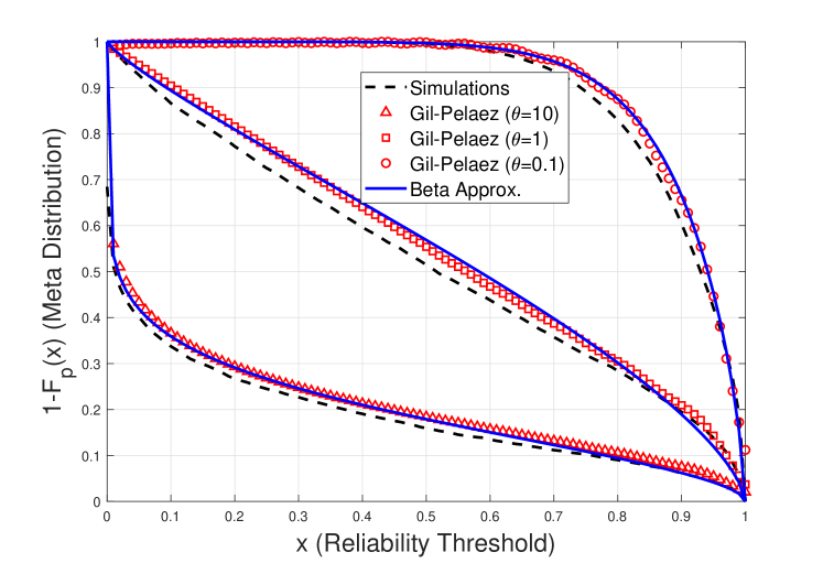
Figure 11: The meta distribution as a function of reliability $x$ for $\theta=\theta_{\mathcal{D}}=\theta_{2}=$10, 1, and 0.1 for SBSs in a $\mu$wave-only network when $B_{1}=B_{2}=1$ and $\alpha_{1}=\alpha_{2}=4$.

IX Conclusion

This paper characterizes the meta distributions of the SIR/SNR and data rate of a typical device in a hybrid spectrum network and $\mu$wave-only network. The meta distribution is evaluated first by formulating and then characterizing the moments of the CSP of a typical device in the hybrid network. Important performance metrics such as the mean local delay, coverage probability, network jitter, and variance of the CSP (or reliability) are studied. Numerical results demonstrate the significance of evaluating the meta distribution which requires a systematic evaluation of the generalized moment of order $b$ that helps in evaluating network metric such as coverage probability when $b=1$, mean local delay when $b=-1$, network jitter using $b=-2$ and $b=-1$, etc. Numerical results provide valuable insights related to the reliability and latency of the hybrid spectrum network and $\mu$wave-only network. These insights would help 5G cellular network operators to find the most efficient operating antenna configuration to achieve certain reliability for certain 5G applications.

Appendix C: Proof of Lemma 4

The $b^{\mathrm{th}}$ moment of the CSP of a typical device served by the mm-wave SBS can be derived as:

$$M_{b,\text{2}}(\theta_{\mathcal{D}})=\mathbb{E}_{l}\bigg{[}\underbrace{\mathbb{P}(n=2|L_{2,min}=l_{2})}_{\bar{\mathcal{A}}_{2}(l_{2})}P_{s,2}(\theta_{\mathcal{D}})^{b}\bigg{]}=\mathbb{E}_{l}\bigg{[}\bar{\mathcal{A}}_{2}(l_{2})\left(p_{L}P_{s,2,L}(\theta_{\mathcal{D}})+p_{N}P_{s,2,N}(\theta_{\mathcal{D}})\right)^{b}\bigg{]},$$

$$\stackrel{{\scriptstyle(a)}}{{=}}\mathbb{E}_{l}\Bigg{[}\bar{\mathcal{A}}_{2}(l_{2})\left(p_{L}\frac{\Gamma\left(m_{L},\frac{m_{L}}{\Omega_{L}}\nu_{L}\right)}{\Gamma{(m_{L})}}+p_{N}\frac{\Gamma\left(m_{N},\frac{m_{N}}{\Omega_{N}}\nu_{N}\right)}{\Gamma(m_{N})}\right)^{b}\Bigg{]},$$

$$\stackrel{{\scriptstyle}}{{=}}\mathbb{E}_{l}\Bigg{[}(\bar{\mathcal{A}}_{2,L}(l_{2,L})+\bar{\mathcal{A}}_{2,N}(l_{2,N}))\times\left(p_{L}\frac{\Gamma\left(m_{L},\frac{m_{L}}{\Omega_{L}}\nu_{L}\right)}{\Gamma{(m_{L})}}+p_{N}\frac{\Gamma\left(m_{N},\frac{m_{N}}{\Omega_{N}}\nu_{N}\right)}{\Gamma(m_{N})}\right)^{b}\Bigg{]},$$

$$\stackrel{{\scriptstyle(b)}}{{=}}\mathbb{E}_{l}\Bigg{[}\bar{\mathcal{A}}_{2,L}(l_{2,L})\left(p_{L}\frac{\Gamma\left(m_{L},\frac{m_{L}}{\Omega_{L}}\nu_{L}\right)}{\Gamma{(m_{L})}}\right)^{b}\Bigg{]}+\mathbb{E}_{l}\Bigg{[}\bar{\mathcal{A}}_{2,N}(l_{2,N})\left(p_{N}\frac{\Gamma\left(m_{N},\frac{m_{N}}{\Omega_{N}}\nu_{N}\right)}{\Gamma(m_{N})}\right)^{b}\Bigg{]},$$

$$\stackrel{{\scriptstyle(c)}}{{=}}\mathbb{E}_{l}\Bigg{[}\bar{\mathcal{A}}_{2,L}(l_{2,L})\,p_{L}^{b}\left(1-\frac{\gamma\left(m_{L},\frac{m_{L}}{\Omega_{L}}\nu_{L}\right)}{\Gamma{(m_{L})}}\right)^{b}\Bigg{]}+\mathbb{E}_{l}\Bigg{[}\bar{\mathcal{A}}_{2,N}(l_{2,N})\,p_{N}^{b}\left(1-\frac{\gamma\left(m_{N},\frac{m_{N}}{\Omega_{N}}\nu_{N}\right)}{\Gamma(m_{N})}\right)^{b}\Bigg{]},$$

$$\stackrel{{\scriptstyle(d)}}{{\approx}}\mathbb{E}_{l}\Bigg{[}\bar{\mathcal{A}}_{2,L}(l_{2,L})p_{L}^{b}\left(1-[1-e^{-\zeta_{L}\nu_{L}}]^{m_{L}}\right)^{b}\Bigg{]}+\mathbb{E}_{l}\Bigg{[}\bar{\mathcal{A}}_{2,N}(l_{2,N})\,p_{N}^{b}\left(1-[1-e^{-\zeta_{N}\nu_{N}}]^{m_{N}}\right)^{b}\Bigg{]},$$

$$\stackrel{{\scriptstyle(e)}}{{=}}\mathbb{E}_{l}\Bigg{[}\bar{\mathcal{A}}_{2,L}(l_{2,L})p_{L}^{b}\sum_{k=0}^{b}\binom{b}{k}\left(-[1-e^{-\zeta_{L}\nu_{L}}]^{m_{L}}\right)^{k}\Bigg{]}+\mathbb{E}_{l}\Bigg{[}\bar{\mathcal{A}}_{2,N}(l_{2,N})\,p_{N}^{b}\sum_{k=0}^{b}\binom{b}{k}\left(-[1-e^{-\zeta_{N}\nu_{N}}]^{m_{N}}\right)^{k}\Bigg{]},$$

$$\stackrel{{\scriptstyle(f)}}{{=}}\mathbb{E}_{l}\Bigg{[}\bar{\mathcal{A}}_{2,L}(l_{2,L})p_{L}^{b}\sum_{k=0}^{b}\sum_{\ddot{k}=0}^{m_{L}k}\binom{b}{k}\binom{m_{L}k}{\ddot{k}}(-1)^{\ddot{k}+k}e^{-\zeta_{L}\nu_{L}\ddot{k}}\Bigg{]}+\mathbb{E}_{l}\Bigg{[}\bar{\mathcal{A}}_{2,N}(l_{2,N})p_{N}^{b}\sum_{k=0}^{b}\sum_{\ddot{k}=0}^{m_{N}k}\binom{b}{k}\binom{m_{N}k}{\ddot{k}}(-1)^{\ddot{k}+k}e^{-\zeta_{N}\nu_{N}\ddot{k}}\Bigg{]},$$

where (a) follows from substituting the value of $P_{s,2,L}(\theta_{\mathcal{D}})$ and $P_{s,2,N}(\theta_{\mathcal{D}})$ from Eq. (16) and Eq. (17), respectively, (b) follows from $l_{\text{2,L}}=r_{2,\mathcal{D}}^{\alpha_{2,L}}$ and $l_{\text{2,N}}=r_{2,\mathcal{D}}^{\alpha_{2,N}}$ and the considered blockage model where $p_{L}=1$ when mm-wave intended link distance $r_{2,\mathcal{D}}<d$ and $p_{N}=1$ when mm-wave intended link distance $r_{2,\mathcal{D}}>d$, (c) follows from $\Gamma(s)=\gamma(s,x)+\Gamma(s,x)$, (d) follows from the CDF of Gamma random variable which can be tightly upper bounded by $\frac{\gamma\left(m_{L},\frac{m_{L}}{\Omega_{L}}\nu_{L}\right)}{\Gamma{(m_{L})}}<[1-e^{-\zeta_{L}\nu_{L}}]^{m_{L}}$ [40], where $\zeta_{L}\overset{\Delta}{=}m_{L}(m_{L}!)^{-1/m_{L}}$, $\nu_{L}\overset{\Delta}{=}\frac{\theta_{\mathcal{D}}r_{2,\mathcal{D}}^{\alpha_{2,L}}\sigma_{2}^{2}}{P_{2}G_{2}}$, $\zeta_{N}\overset{\Delta}{=}m_{N}(m_{N}!)^{-1/m_{N}}$, and $\nu_{N}\overset{\Delta}{=}\frac{\theta_{\mathcal{D}}r_{2,\mathcal{D}}^{\alpha_{2,N}}\sigma_{2}^{2}}{P_{2}G_{2}}$ [16]. The steps in (e) and (f) are done by following the binomial expansion theorem. Finally, the Lemma 4 follows from de-conditioning on $l$ and using the definitions $\ddot{\nu_{L}}\overset{\Delta}{=}\frac{\nu_{L}}{r_{2,\mathcal{D}}^{\alpha_{2,L}}}=\frac{\nu_{L}}{l_{\text{2,L}}}=\frac{\theta_{\mathcal{D}}\sigma_{2}^{2}}{P_{2}G_{2}}$ and $\ddot{\nu_{N}}\overset{\Delta}{=}\frac{\nu_{N}}{r_{2,\mathcal{D}}^{\alpha_{2,N}}}=\frac{\nu_{N}}{l_{\text{2,N}}}=\frac{\theta_{\mathcal{D}}\sigma_{2}^{2}}{P_{2}G_{2}}$.

Appendix D: Proof of Lemma 5

The $b^{\mathrm{th}}$ moment of the CSP of a typical device when associated to $\mu$wave MBS is derived as follows:

$$M_{b,\text{1}}(\theta_{\mathcal{D}})=\mathbb{E}_{l_{1}}\bigg{[}\underbrace{\mathbb{P}(n=1|L_{1,min}=l_{1})}_{\bar{\mathcal{A}}_{1}(l_{1})}P_{s,1}(\theta_{\mathcal{D}})^{b}\bigg{]}\stackrel{{\scriptstyle(a)}}{{=}}\mathbb{E}_{l_{1}}\bigg{[}\bar{\mathcal{A}}_{1}(l_{1})\prod_{\mathbf{y}_{1,i}\in\mathbf{\Phi}_{1}\backslash\{\mathbf{y}_{1,0}\}}\frac{1}{\left(1+\theta_{\mathcal{D}}\left(\frac{r_{1,\mathcal{D}}}{\|\mathbf{y}_{1,i}\|}\right)^{\alpha_{1}}\right)^{b}}\bigg{]},$$

$$\stackrel{{\scriptstyle(b)}}{{=}}\mathbb{E}_{l_{1}}\bigg{[}\bar{\mathcal{A}}_{1}(l_{1})\exp\left(\int_{r}^{\infty}-2\lambda_{1}\pi\bigg{[}1-\frac{1}{\left(1+\theta_{\mathcal{D}}\left(\frac{r}{y}\right)^{\alpha_{1}}\right)^{b}}\bigg{]}y\text{d}y\right)\bigg{]}\stackrel{{\scriptstyle(c)}}{{=}}\mathbb{E}_{l_{1}}\bigg{[}\bar{\mathcal{A}}_{1}(l_{1})\exp\left(\int_{l_{1}^{\frac{1}{\alpha_{1}}}}^{\infty}-2\lambda_{1}\pi\bigg{[}1-\frac{1}{\left(1+\theta_{\mathcal{D}}\frac{l_{1}}{y^{\alpha_{1}}}\right)^{b}}\bigg{]}y\text{d}y\right),$$

$$\stackrel{{\scriptstyle(d)}}{{=}}\mathbb{E}_{l_{1}}\bigg{[}\bar{\mathcal{A}}_{1}(l_{1})\exp\left(\int_{0}^{1}-2\lambda_{1}\pi\bigg{[}1-\frac{1}{\left(1+\theta_{\mathcal{D}}v\right)^{b}}\bigg{]}v^{-1}\frac{y^{2}}{\alpha_{1}}\text{d}v\right)\bigg{]},$$

$$\stackrel{{\scriptstyle(e)}}{{=}}\mathbb{E}_{l_{1}}\bigg{[}\bar{\mathcal{A}}_{1}(l_{1})\exp\left(\frac{-2\lambda_{1}\pi l_{1}^{\frac{2}{\alpha_{1}}}}{\alpha_{1}}\int_{0}^{1}\bigg{[}1-\frac{1}{\left(1+\theta_{\mathcal{D}}v\right)^{b}}\bigg{]}\frac{1}{v^{\frac{2}{\alpha_{1}}+1}}\text{d}v\right)\Bigg{]},$$

where (a) follows from taking expectation over $l_{1}=r^{\alpha_{1}}$ and considering the conditional association probability for the typical device connecting to the MBSs tier given in Lemma (1) and substituting the value of $P_{s,1}(\theta_{\mathcal{D}})$ from Eq. (V-C). In step (b) we apply PGFL of the PPP [41, Chapter 4]. Step (c) follows from averaging over $l_{1}$. In step (d), we use the change of variable $v=\frac{l_{1}}{y^{\alpha_{1}}}$, $dy=\frac{-1}{\alpha_{1}l_{1}y^{-\alpha_{1}-1}}dv=\frac{-1}{\alpha_{1}}v^{-1}ydv$, when $y=l_{1}^{\frac{1}{\alpha_{1}}}$ $\rightarrow$ $v=1$ and when $y=\infty$ $\rightarrow$ $v=0$ and we swap the integral limits and multiply by $-1$, (e) follows from $y^{2}=l_{1}^{\frac{2}{\alpha_{1}}}/v^{\frac{2}{\alpha_{1}}}$ and doing some mathematical manipulations.

Appendix E: Proof of Lemma 6

While taking the association biases effect in consideration, the $b^{\mathrm{th}}$ moment of the CSP $P_{s,k}(\theta_{\mathcal{D}})$ of the typical device when it is served by the $k^{\mathrm{th}}$ tier is given as follows:

$$M_{b,\text{k'}}(\theta_{\mathcal{D}})=\mathbb{E}_{r_{k,\mathcal{D}}}\bigg{[}\mathbb{P}(n=k|r_{k,\mathcal{D}})P_{s,k^{\prime}}(\theta_{\mathcal{D}})^{b}\bigg{]},$$

$$\stackrel{{\scriptstyle(a)}}{{=}}\mathbb{E}_{r_{k,\mathcal{D}}}\bigg{[}\prod_{j\neq k}e^{-\pi\lambda_{j}(\hat{P}_{jk}\hat{B}_{jk})^{2/\alpha_{j}}r^{2}}\times\prod_{\mathbf{y}_{k,i}\in\mathbf{\Phi}_{k}\backslash\{\mathbf{y}_{k,0}\}}\frac{1}{\left(1+\theta_{\mathcal{D}}\left(\frac{r_{k,\mathcal{D}}}{\|\mathbf{y}_{k,i}\|}\right)^{\alpha_{k}}\right)^{b}}\bigg{]},$$

$$\stackrel{{\scriptstyle(b)}}{{=}}\mathbb{E}_{r_{k,\mathcal{D}}}\bigg{[}\prod_{j\neq k}e^{-\pi\lambda_{j}(\hat{P}_{jk}\hat{B}_{jk})^{2/\alpha_{j}}r^{2}}\times\exp\left(\int_{r_{k,\mathcal{D}}}^{\infty}-2\lambda_{k}\pi\bigg{[}1-\frac{1}{\left(1+\theta_{\mathcal{D}}\left(\frac{r_{k,\mathcal{D}}}{y}\right)^{\alpha_{k}}\right)^{b}}\bigg{]}y\text{d}y\right)\bigg{]},$$

$$\stackrel{{\scriptstyle(c)}}{{=}}\int_{0}^{\infty}2\lambda_{k}\pi re^{-\lambda_{k}\pi r^{2}}e^{-\sum\limits_{j\neq k}\lambda_{j}(\hat{P}_{jk}\hat{B}_{jk})^{2/\alpha_{j}}\pi r^{2}}\times\exp\left(\int_{r}^{\infty}-2\lambda_{k}\pi\bigg{[}1-\frac{1}{\left(1+\theta_{\mathcal{D}}\left(\frac{r}{y}\right)^{\alpha_{k}}\right)^{b}}\bigg{]}y\text{d}y\right)\text{d}r,$$

$$\stackrel{{\scriptstyle(d)}}{{=}}\int_{0}^{\infty}e^{-q}e^{-q\sum\limits_{j\neq k}\hat{\lambda}_{jk}(\hat{P}_{jk}\hat{B}_{jk})^{2/\alpha_{j}}}\times\exp\left(-2q\int_{0}^{1}\bigg{[}1-\frac{1}{\left(1+\theta_{\mathcal{D}}v^{\alpha_{k}}\right)^{b}}\bigg{]}v^{-3}\text{d}v\right)\text{d}q,$$

$$\stackrel{{\scriptstyle(e)}}{{=}}\int_{0}^{\infty}e^{-q}e^{-q\sum\limits_{j\neq k}\hat{\lambda}_{jk}(\hat{P}_{jk}\hat{B}_{jk})^{2/\alpha_{j}}}\times\exp\left(-q\int_{1}^{\infty}\bigg{[}1-\frac{1}{\left(1+\theta_{\mathcal{D}}u^{-\alpha_{k}/2}\right)^{b}}\bigg{]}\text{d}u\right)\text{d}q,$$

$$\stackrel{{\scriptstyle(f)}}{{=}}\int_{0}^{\infty}e^{-q}e^{-q\sum\limits_{j\neq k}\hat{\lambda}_{jk}(\hat{P}_{jk}\hat{B}_{jk})^{2/\alpha_{j}}}\times\exp\left(-q\bigg{[}\text{ }_{2}F_{1}(b,-\frac{2}{\alpha_{k}};1-\frac{2}{\alpha_{k}};-\theta_{\mathcal{D}})-1\bigg{]}\right)\text{d}q,$$

$$=\frac{1}{\sum\limits_{j\neq k}\hat{\lambda}_{jk}(\hat{P}_{jk}\hat{B}_{jk})^{2/\alpha_{j}}+\text{ }_{2}F_{1}(b,-\frac{2}{\alpha_{k}};1-\frac{2}{\alpha_{k}};-\theta_{\mathcal{D}})}.$$

where (a) follows from considering the conditional association probability for the typical device connecting to the $k^{\mathrm{th}}$ tier given in Eq. (30). In step (b), we apply PGFL of the PPP [41, Chapter 4]. Step (c) follows from averaging over $r_{k,\mathcal{D}}$, step (d) is by using variable substitution $q=\pi\lambda_{k}r^{2}$ and $v=r/y$. In step (e), we perform variable substitution $v=u(\hat{P}_{jk}\hat{B}_{jk})^{-1/\alpha_{j}}$ and step (f) follows from the fact that $\text{ }_{2}F_{1}(b,-\frac{2}{\alpha};1-\frac{2}{\alpha};-\theta)\equiv 1+\int_{1}^{\infty}(1-\frac{1}{(1+\theta h^{-\alpha/2})^{b}})\text{d}h$.

References

- [1] H. Ibrahim, H. Tabassum, and U. T. Nguyen, “Meta distribution of SIR in dual-hop Internet-of-Things (IoT) networks,” IEEE International Conference on Communications (ICC), May 2019.
- [2] 3GPP, “Study on new radio (NR) access technology - physical layer aspects,” TR 38.802 (Rel. 14), 2017.
- [3] H. Elshaer, M. N. Kulkarni, F. Boccardi, J. G. Andrews, and M. Dohler, “Downlink and uplink cell association with traditional macrocells and millimeter wave small cells,” IEEE Transactions on Wireless Communications, vol. 15, no. 9, pp. 6244–6258, 2016.
- [4] O. Semiari, W. Saad, M. Bennis, and M. Debbah, “Integrated millimeter wave and sub-6 GHz wireless networks: A roadmap for joint mobile broadband and ultra-reliable low-latency communications,” IEEE Wireless Communications, 2019.
- [5] H. Ji, S. Park, J. Yeo, Y. Kim, J. Lee, and B. Shim, “Ultra-reliable and low-latency communications in 5G downlink: Physical layer aspects,” IEEE Wireless Communications, vol. 25, no. 3, pp. 124–130, 2018.
- [6] J. G. Andrews, S. Buzzi, W. Choi, S. V. Hanly, A. Lozano, A. C. Soong, and J. C. Zhang, “What will 5G be?” IEEE Journal on selected areas in communications, vol. 32, no. 6, pp. 1065–1082, 2014.
- [7] P. Wang, Y. Li, L. Song, and B. Vucetic, “Multi-gigabit millimeter wave wireless communications for 5G: From fixed access to cellular networks,” IEEE Communications Magazine, vol. 53, no. 1, pp. 168–178, 2015.
- [8] M. Polese, M. Giordani, M. Mezzavilla, S. Rangan, and M. Zorzi, “Improved handover through dual connectivity in 5G mmwave mobile networks,” IEEE Journal on Selected Areas in Communications, vol. 35, no. 9, pp. 2069–2084, 2017.
- [9] M. Haenggi, “The meta distribution of the SIR in Poisson bipolar and cellular networks,” IEEE Transactions on Wireless Communications, vol. 15, no. 4, pp. 2577–2589, 2016.
- [10] M. Bennis, M. Debbah, and H. V. Poor, “Ultrareliable and low-latency wireless communication: Tail, risk, and scale,” Proceedings of the IEEE, vol. 106, no. 10, pp. 1834–1853, 2018.
- [11] S. S. Kalamkar and M. Haenggi, “Per-link reliability and rate control: Two facets of the SIR meta distribution,” IEEE Wireless Communications Letters, 2019.
- [12] M. Salehi, A. Mohammadi, and M. Haenggi, “Analysis of D2D underlaid cellular networks: SIR meta distribution and mean local delay,” IEEE Transactions on Communications, vol. 65, no. 7, pp. 2904–2916, 2017.
- [13] M. Salehi, H. Tabassum, and E. Hossain, “Meta distribution of sir in large-scale uplink and downlink NOMA networks,” IEEE Transactions on Communications, 2018.
- [14] N. Deng and M. Haenggi, “The energy and rate meta distributions in wirelessly powered D2D networks,” IEEE Journal on Selected Areas in Communications, vol. 37, no. 2, pp. 269–282, 2019.
- [15] M. Di Renzo, “Stochastic geometry modeling and analysis of multi-tier millimeter wave cellular networks,” IEEE Transactions on Wireless Communications, vol. 14, no. 9, pp. 5038–5057, 2015.
- [16] T. Bai and R. W. Heath, “Coverage and rate analysis for millimeter-wave cellular networks,” IEEE Transactions on Wireless Communications, vol. 14, no. 2, pp. 1100–1114, 2015.
- [17] E. Turgut and M. C. Gursoy, “Coverage in heterogeneous downlink millimeter wave cellular networks,” IEEE Transactions on Communications, vol. 65, no. 10, pp. 4463–4477, 2017.
- [18] N. Deng, Y. Sun, and M. Haenggi, “Success probability of millimeter-wave D2D networks with heterogeneous antenna arrays,” in Wireless Communications and Networking Conference (WCNC). IEEE, 2018, pp. 1–5.
- [19] S. Singh, M. N. Kulkarni, A. Ghosh, and J. G. Andrews, “Tractable model for rate in self-backhauled millimeter wave cellular networks,” IEEE Journal on Selected Areas in Communications, vol. 33, no. 10, pp. 2196–2211, 2015.
- [20] N. Deng and M. Haenggi, “A fine-grained analysis of millimeter-wave device-to-device networks,” IEEE Trans. Commun, vol. 65, no. 11, pp. 4940–4954, 2017.
- [21] A. Ghosh, T. A. Thomas, M. C. Cudak, R. Ratasuk, P. Moorut, F. W. Vook, T. S. Rappaport, G. R. MacCartney, S. Sun, and S. Nie, “Millimeter-wave enhanced local area systems: A high-data-rate approach for future wireless networks,” IEEE Journal on Selected Areas in Communications, vol. 32, no. 6, pp. 1152–1163, 2014.
- [22] J. G. Andrews, T. Bai, M. N. Kulkarni, A. Alkhateeb, A. K. Gupta, and R. W. Heath, “Modeling and analyzing millimeter wave cellular systems,” IEEE Transactions on Communications, vol. 65, no. 1, pp. 403–430, 2017.
- [23] H. Ibrahim, H. ElSawy, U. T. Nguyen, and M.-S. Alouini, “Modeling virtualized downlink cellular networks with ultra-dense small cells,” in IEEE International Conference on Communications (ICC), 2015, pp. 5360–5366.
- [24] H. Ibrahim, W. Bao, and U. T. Nguyen, “Data rate utility analysis for uplink two-hop internet-of-things networks,” IEEE Internet of Things Journal, 2018.
- [25] H. Ibrahim, H. ElSawy, U. T. Nguyen, and M.-S. Alouini, “Mobility-aware modeling and analysis of dense cellular networks with C-plane/U-plane split architecture,” IEEE Transactions on Communications, vol. 64, no. 11, pp. 4879–4894, 2016.
- [26] G. R. MacCartney, J. Zhang, S. Nie, and T. S. Rappaport, “Path loss models for 5G millimeter wave propagation channels in urban microcells.” in Globecom, 2013, pp. 3948–3953.
- [27] T. A. Khan, A. Alkhateeb, and R. W. Heath, “Millimeter wave energy harvesting,” IEEE Transactions on Wireless Communications, vol. 15, no. 9, pp. 6048–6062, 2016.
- [28] W. Yi, Y. Liu, and A. Nallanathan, “Modeling and analysis of D2D millimeter-wave networks with poisson cluster processes,” IEEE Transactions on Communications, vol. 65, no. 12, pp. 5574–5588, 2017.
- [29] M. Nakagami, “The m-distribution: A general formula of intensity distribution of rapid fading,” in Statistical methods in radio wave propagation. Elsevier, 1960, pp. 3–36.
- [30] M. K. Simon and M.-S. Alouini, Digital communication over fading channels. John Wiley & Sons, 2005, vol. 95.
- [31] K. Venugopal, M. C. Valenti, and R. W. Heath, “Device-to-device millimeter wave communications: Interference, coverage, rate, and finite topologies,” IEEE Transactions on Wireless Communications, vol. 15, no. 9, pp. 6175–6188, 2016.
- [32] T. Bai, R. Vaze, and R. W. Heath, “Analysis of blockage effects on urban cellular networks,” IEEE Transactions on Wireless Communications, vol. 13, no. 9, pp. 5070–5083, 2014.
- [33] J. Gil-Pelaez, “Note on the inversion theorem,” Biometrika, vol. 38, no. 3-4, pp. 481–482, 1951.
- [34] “Supplementary appendices-technical report. [online],” \hrefhttps://www.dropbox.com/s/ls25g6o43m9xdq6/Metacoexisting.pdf?dl=0https://www.dropbox.com/s/ls25g6o43m9xdq6/Meta-coexisting.pdf?dl=0.
- [35] R. K. Ganti and M. Haenggi, “Asymptotics and approximation of the SIR distribution in general cellular networks,” IEEE Transactions on Wireless Communications, vol. 15, no. 3, pp. 2130–2143, 2016.
- [36] Y. Wang, M. Haenggi, and Z. Tan, “The meta distribution of the SIR for cellular networks with power control,” IEEE Transactions on Communications, vol. 66, no. 4, pp. 1745–1757, 2018.
- [37] M. Kronenburg, “The binomial coefficient for negative arguments,” arXiv preprint arXiv:1105.3689, 2011.
- [38] H.-S. Jo, Y. J. Sang, P. Xia, and J. G. Andrews, “Heterogeneous cellular networks with flexible cell association: A comprehensive downlink SINR analysis,” IEEE Transactions on Wireless Communications, vol. 11, no. 10, pp. 3484–3495, 2012.
- [39] Y. Wang, M. Haenggi, and Z. Tan, “Sir meta distribution of k-tier downlink heterogeneous cellular networks with cell range expansion,” IEEE Transactions on Communications, 2018.
- [40] H. Alzer, “On some inequalities for the incomplete gamma function,” Mathematics of Computation of the American Mathematical Society, vol. 66, no. 218, pp. 771–778, 1997.
- [41] M. Haenggi, Stochastic geometry for wireless networks. Cambridge University Press, 2012.