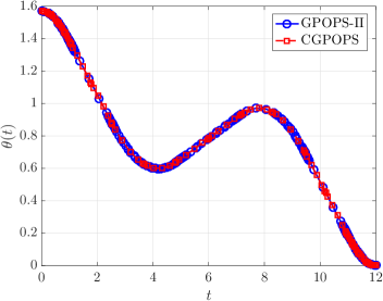
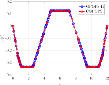
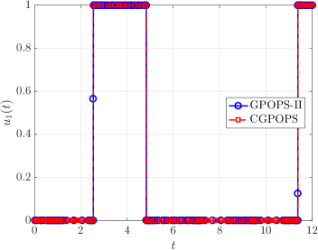
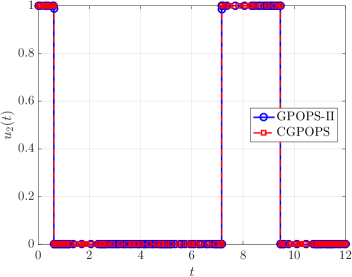
โ„‚โ€‹๐”พโ€‹โ„™โ€‹๐•†โ€‹โ„™โ€‹๐•Šโ„‚๐”พโ„™๐•†โ„™๐•Š{\mathbb{CGPOPS}}: A C++ Software for Solving Multiple-Phase Optimal Control Problems Using Adaptive Gaussian Quadrature Collocation and Sparse Nonlinear Programming

Yunus M.ย Agamawi
Anil V.ย Rao
University of Florida
Gainesville, FL, 32611-6250
Ph.D.ย Student, Department of Mechanical and Aerospace Engineering. E-mail: yagamawi@ufl.edu.Associate Professor, Department of Mechanical and Aerospace Engineering, Erich Farber Faculty Fellow and University Term Professor. E-mail: anilvrao@ufl.edu. Associate Fellow, AIAA. Corresponding Author.
Abstract

A general-purpose C++ software program called โ„‚โ€‹๐”พโ€‹โ„™โ€‹๐•†โ€‹โ„™โ€‹๐•Šโ„‚๐”พโ„™๐•†โ„™๐•Š\mathbb{CGPOPS} is described for solving multiple-phase optimal control problems using adaptive Gaussian quadrature collocation. The software employs a Legendre-Gauss-Radau direct orthogonal collocation method to transcribe the continuous-time optimal control problem into a large sparse nonlinear programming problem. A class of hโ€‹pโ„Ž๐‘hp mesh refinement methods are implemented which determine the number of mesh intervals and the degree of the approximating polynomial within each mesh interval to achieve a specified accuracy tolerance. The software is interfaced with the open source Newton NLP solver IPOPT. All derivatives required by the NLP solver are computed using either central finite differencing, bicomplex-step derivative approximation, hyper-dual derivative approximation, or automatic differentiation. The key components of the software are described in detail and the utility of the software is demonstrated on five optimal control problems of varying complexity. The software described in this article provides a computationally efficient and accurate approach for solving a wide variety of complex constrained optimal control problems.

1 Introduction

Optimal control problems arise in a wide variety of subjects including virtually all branches of engineering, economics, and medicine. Over the past few decades, the subject of optimal control has transitioned from theory to computations as a result of the increasing complexity of optimal control applications and the inability to solve them analytically. In particular, computational optimal control has become a science in and of itself, resulting in a variety of numerical methods and corresponding software implementations of those methods. To date, the vast majority of software implementations of optimal control involve direct transcription of a continuous optimal control problem to a nonlinear programming problem (NLP). The resulting NLP from discretizing the continuous optimal control problem may then be solved using well established techniques. Examples of well-known software for solving optimal control problems include SOCS [1], DIRCOL [2], GESOP [3], OTIS [4], MISER [5], PSOPT [6], GPOPS [7], ICLOCS [8], ACADO [9], and ๐”พโ€‹โ„™โ€‹๐•†โ€‹โ„™โ€‹๐•Šโˆ’๐•€โ€‹๐•€๐”พโ„™๐•†โ„™๐•Š๐•€๐•€\mathbb{GPOPS-II} [10].

Over the past few decades, direct collocation methods have become popular in the numerical solution of nonlinear optimal control problems. In a direct collocation method, the state and control are parameterized at an appropriately chosen set of discrete points along the time interval of interest. The continuous optimal control problem is then transcribed to a finite-dimensional NLP. The resulting NLP may then be solved using well known software such as SNOPT [11], IPOPT [12], and KNITRO [13]. Direct collocation methods were originally developed as hโ„Žh methods (such as Euler or Runge-Kutta methods) where the time interval of interest is divided into a mesh and the state is approximated using a fixed-degree polynomial in each mesh interval. Convergence in an hโ„Žh method is then achieved by increasing the number and placement of the mesh points [14, 15, 16]. More recently, a great deal of research has been done in the class of direct Gaussian quadrature orthogonal collocation methods [17, 18, 19, 20, 21, 22, 7, 23, 24, 25, 26, 27, 28]. In a Gaussian quadrature collocation method, the state is typically approximated using a Lagrange polynomial where the support points of the Lagrange polynomial are chosen to be points associated with a Gaussian quadrature. Originally, Gaussian quadrature collocation methods were implemented as p๐‘p methods using a single interval. Convergence of the p๐‘p method was then achieved by increasing the degree of the polynomial approximation. For problems whose solutions are smooth and well-behaved, a Gaussian quadrature orthogonal collocation method converges at an exponential rate [29, 30, 31, 32, 33]. The most well developed p๐‘p Gaussian quadrature methods are those that employ either Legendre-Gauss (LG) points [19, 7], Legendre-Gauss-Radau (LGR) points [26, 23, 24], or Legendre-Gauss-Lobatto (LGL) points [17].

In this paper a new optimal control software called โ„‚โ€‹๐”พโ€‹โ„™โ€‹๐•†โ€‹โ„™โ€‹๐•Šโ„‚๐”พโ„™๐•†โ„™๐•Š{\mathbb{CGPOPS}} is described that employs hโ€‹pโ„Ž๐‘hp direct orthogonal collocation methods. An hโ€‹pโ„Ž๐‘hp method is a hybrid between an hโ„Žh and a p๐‘p method in that both the number of mesh intervals and the degree of the approximating polynomial within each mesh interval can be varied in order to achieve a specified accuracy. As a result, in an hโ€‹pโ„Ž๐‘hp method it is possible to take advantage of the exponential convergence of a Gaussian quadrature method in regions where the solution is smooth and introduce mesh points only when necessary to deal with potential nonsmoothness or rapidly changing behavior in the solution. Originally, hโ€‹pโ„Ž๐‘hp methods were developed as finite-element methods for solving partial differential equations [34, 35, 36, 37]. In the past few years the problem of developing hโ€‹pโ„Ž๐‘hp methods for solving optimal control problems has been of interest [38, 39, 40, 41, 42]. The work of [38, 39, 40, 41, 42] provides examples of the benefits of using an hโ€‹pโ„Ž๐‘hp-adaptive method over either a p๐‘p method or an hโ„Žh method. This recent research has shown that convergence using hโ€‹pโ„Ž๐‘hp methods can be achieved with a significantly smaller finite-dimensional approximation than would be required when using either an hโ„Žh or a p๐‘p method.

It is noted that previously the software ๐”พโ€‹โ„™โ€‹๐•†โ€‹โ„™โ€‹๐•Šโˆ’๐•€โ€‹๐•€๐”พโ„™๐•†โ„™๐•Š๐•€๐•€\mathbb{GPOPS-II} was developed as described in Ref.ย [10]. Although both the ๐”พโ€‹โ„™โ€‹๐•†โ€‹โ„™โ€‹๐•Šโˆ’๐•€โ€‹๐•€๐”พโ„™๐•†โ„™๐•Š๐•€๐•€\mathbb{GPOPS-II} and โ„‚โ€‹๐”พโ€‹โ„™โ€‹๐•†โ€‹โ„™โ€‹๐•Šโ„‚๐”พโ„™๐•†โ„™๐•Š{\mathbb{CGPOPS}} software programs implement Gaussian quadrature collocation with hโ€‹pโ„Ž๐‘hp mesh refinement, โ„‚โ€‹๐”พโ€‹โ„™โ€‹๐•†โ€‹โ„™โ€‹๐•Šโ„‚๐”พโ„™๐•†โ„™๐•Š{\mathbb{CGPOPS}} is a fundamentally different software from ๐”พโ€‹โ„™โ€‹๐•†โ€‹โ„™โ€‹๐•Šโˆ’๐•€โ€‹๐•€๐”พโ„™๐•†โ„™๐•Š๐•€๐•€\mathbb{GPOPS-II}. First, ๐”พโ€‹โ„™โ€‹๐•†โ€‹โ„™โ€‹๐•Šโˆ’๐•€โ€‹๐•€๐”พโ„™๐•†โ„™๐•Š๐•€๐•€\mathbb{GPOPS-II} is a MATLAB software program, while โ„‚โ€‹๐”พโ€‹โ„™โ€‹๐•†โ€‹โ„™โ€‹๐•Šโ„‚๐”พโ„™๐•†โ„™๐•Š{\mathbb{CGPOPS}} is a C++ software program. Furthermore, because โ„‚โ€‹๐”พโ€‹โ„™โ€‹๐•†โ€‹โ„™โ€‹๐•Šโ„‚๐”พโ„™๐•†โ„™๐•Š{\mathbb{CGPOPS}} is implemented in C++, it has the potential for improved computational efficiency and portability over a MATLAB software such as ๐”พโ€‹โ„™โ€‹๐•†โ€‹โ„™โ€‹๐•Šโˆ’๐•€โ€‹๐•€๐”พโ„™๐•†โ„™๐•Š๐•€๐•€\mathbb{GPOPS-II}. Second, while ๐”พโ€‹โ„™โ€‹๐•†โ€‹โ„™โ€‹๐•Šโˆ’๐•€โ€‹๐•€๐”พโ„™๐•†โ„™๐•Š๐•€๐•€\mathbb{GPOPS-II} employs both sparse finite-differencing and automatic differentiation using the software ADiGatorย [43], โ„‚โ€‹๐”พโ€‹โ„™โ€‹๐•†โ€‹โ„™โ€‹๐•Šโ„‚๐”พโ„™๐•†โ„™๐•Š{\mathbb{CGPOPS}} employs the following four derivative estimation methods: central finite differencing, bicomplex-stepย [44], hyper-dualย [45], and automatic differentiationย [46]. Both the bicomplex-step and hyper-dual derivative approximations are referred to as semi-automatic differentiation methods and are implemented via source code transformation and operator overloading. Third, while ๐”พโ€‹โ„™โ€‹๐•†โ€‹โ„™โ€‹๐•Šโˆ’๐•€โ€‹๐•€๐”พโ„™๐•†โ„™๐•Š๐•€๐•€\mathbb{GPOPS-II} is only capable of identifying the first-order derivative dependencies and over-estimates the dependencies of the second derivatives, โ„‚โ€‹๐”พโ€‹โ„™โ€‹๐•†โ€‹โ„™โ€‹๐•Šโ„‚๐”พโ„™๐•†โ„™๐•Š{\mathbb{CGPOPS}} is able to exactly identify both the first- and second-order derivative dependencies of the continuous optimal control problem functions when the derivatives are approximated using the hyper-dual method. The improvement in determining the dependencies at the level of second derivatives further improves computational efficiency over ๐”พโ€‹โ„™โ€‹๐•†โ€‹โ„™โ€‹๐•Šโˆ’๐•€โ€‹๐•€๐”พโ„™๐•†โ„™๐•Š๐•€๐•€\mathbb{GPOPS-II}.

The objective of this paper is to describe a computationally efficient general-purpose C++ optimal control software that accurately solves a wide variety of constrained continuous optimal control problems. In particular, the software described in this paper employs a differential form of the multiple-interval version of the Legendre-Gauss-Radau (LGR) collocation method [23, 24, 25, 28]. The LGR collocation method is chosen for use in the software because it provides highly accurate state, control, and costate approximations while maintaining a relatively low-dimensional approximation of the continuous problem. The key components of the software are then described and the software is demonstrated on five examples from the open literature. Each example demonstrates different capabilities of the software. The first example is the hyper-sensitive optimal control problem from Ref.ย [47] and demonstrates the ability of the software to accurately solve a problem whose optimal solution changes rapidly in particular regions of the solution. The second example is the reusable launch vehicle entry problem taken from Ref.ย [14] and demonstrates the ability of โ„‚โ€‹๐”พโ€‹โ„™โ€‹๐•†โ€‹โ„™โ€‹๐•Šโ„‚๐”พโ„™๐•†โ„™๐•Š{\mathbb{CGPOPS}} to compute an accurate solution using a relatively coarse mesh. The third example is the space station attitude control problem taken from Refs.ย [48, 14] and demonstrates the ability of the software to generate accurate solutions to a problem whose solution is not intuitive. The fourth example is a free-flying robot problem taken from Refs.ย [14, 49] and shows the ability of the software to handle bang-bang optimal control problems using the novel bang-bang control mesh refinement method included in the software. The fifth example is a launch vehicle ascent problem taken from Refs.ย [50, 7, 14] that demonstrates the ability of the software to solve a multiple-phase optimal control problem. In order to validate the results, the solutions obtained using โ„‚โ€‹๐”พโ€‹โ„™โ€‹๐•†โ€‹โ„™โ€‹๐•Šโ„‚๐”พโ„™๐•†โ„™๐•Š{\mathbb{CGPOPS}} are compared against the solutions obtained using the software โ„‚โ€‹๐”พโ€‹โ„™โ€‹๐•†โ€‹โ„™โ€‹๐•Šโ„‚๐”พโ„™๐•†โ„™๐•Š\mathbb{CGPOPS} [10].

This paper is organized as follows. In Section 2 the general multiple-phase optimal control problem is present. In Section 3 the Legendre-Gauss-Radau collocation method that is used as the basis of โ„‚โ€‹๐”พโ€‹โ„™โ€‹๐•†โ€‹โ„™โ€‹๐•Šโ„‚๐”พโ„™๐•†โ„™๐•Š{\mathbb{CGPOPS}} is described. In Section 4 the key components of โ„‚โ€‹๐”พโ€‹โ„™โ€‹๐•†โ€‹โ„™โ€‹๐•Šโ„‚๐”พโ„™๐•†โ„™๐•Š{\mathbb{CGPOPS}} are described. In Section 5 the results obtained using the software on the five aforementioned examples are shown. In Section 6 a discussion of the capabilities of the software that are demonstrated by the results obtained using the software is provided. In Section 7 possible limitations of the software are discussed. Finally, in Section 8 conclusions on the work described in this paper are provided.

2 General Multiple-Phase Optimal Control Problems

The general multiple-phase optimal control problem that can be solved by โ„‚โ€‹๐”พโ€‹โ„™โ€‹๐•†โ€‹โ„™โ€‹๐•Šโ„‚๐”พโ„™๐•†โ„™๐•Š{\mathbb{CGPOPS}} is given as follows. Without loss of generality, consider the following general multiple-phase optimal control problem where each phase is defined on the interval tโˆˆ[t0(p),tf(p)]๐‘กsuperscriptsubscript๐‘ก0๐‘superscriptsubscript๐‘ก๐‘“๐‘t\in[t_{0}^{(p)},t_{f}^{(p)}]. First let pโˆˆ{1,โ€ฆ,P}๐‘1โ€ฆ๐‘ƒp\in\{1,\dots,P\} be the phase number where P๐‘ƒP is the total number of phases. Determine the state ๐ฒ(p)โ€‹(t)โˆˆโ„1ร—ny(p)superscript๐ฒ๐‘๐‘กsuperscriptโ„1superscriptsubscript๐‘›๐‘ฆ๐‘{\bf{y}}^{(p)}(t)\in\mathbb{R}^{1~{}\times~{}n_{y}^{(p)}}, the control ๐ฎ(p)โ€‹(t)โˆˆโ„1ร—nu(p)superscript๐ฎ๐‘๐‘กsuperscriptโ„1superscriptsubscript๐‘›๐‘ข๐‘{\bf{u}}^{(p)}(t)\in\mathbb{R}^{1~{}\times~{}n_{u}^{(p)}}, the integrals ๐ช(p)โˆˆโ„1ร—nq(p)superscript๐ช๐‘superscriptโ„1superscriptsubscript๐‘›๐‘ž๐‘{\bf{q}}^{(p)}\in\mathbb{R}^{1~{}\times~{}n_{q}^{(p)}}, the start times t0(p)โˆˆโ„superscriptsubscript๐‘ก0๐‘โ„t_{0}^{(p)}\in\mathbb{R}, and the terminus times tf(p)โˆˆโ„superscriptsubscript๐‘ก๐‘“๐‘โ„t_{f}^{(p)}\in\mathbb{R} in all phases pโˆˆ{1,โ€ฆ,P}๐‘1โ€ฆ๐‘ƒp\in\{1,\dots,P\}, along with the static parameters ๐ฌโˆˆโ„1ร—ns๐ฌsuperscriptโ„1subscript๐‘›๐‘ {\bf{s}}\in\mathbb{R}^{1~{}\times~{}n_{s}} that minimize the objective functional

๐’ฅ=ฯ•โ€‹(๐ž(1),โ€ฆ,๐ž(๐’ซ),๐ฌ),๐’ฅitalic-ฯ•superscript๐ž1โ€ฆsuperscript๐ž๐’ซ๐ฌ\cal{J}=\cal{\phi}\left({\bf{e}}^{(1)},\dots,{\bf{e}}^{(P)},{\bf{s}}\right)~{}, (1)

subject to the dynamic constraints

dโ€‹๐ฒ(p)dโ€‹tโ‰ก๐ฒห™(p)=๐š(p)โ€‹(๐ฒ(p)โ€‹(t),๐ฎ(p)โ€‹(t),t,๐ฌ),pโˆˆ{1,โ€ฆ,P},formulae-sequence๐‘‘superscript๐ฒ๐‘๐‘‘๐‘กsuperscriptห™๐ฒ๐‘superscript๐š๐‘superscript๐ฒ๐‘๐‘กsuperscript๐ฎ๐‘๐‘ก๐‘ก๐ฌ๐‘1โ€ฆ๐‘ƒ\frac{d{\bf{y}}^{(p)}}{dt}\equiv\dot{{\bf{y}}}^{(p)}={\bf{a}}^{(p)}\left({\bf{y}}^{(p)}(t),{\bf{u}}^{(p)}(t),t,{\bf{s}}\right)~{},\quad p\in\{1,\dots,P\}~{}, (2)

the event constraints

๐›minโ‰ค๐›โ€‹(๐ž(1),โ€ฆ,๐ž(P),๐ฌ)โ‰ค๐›max,subscript๐›๐›superscript๐ž1โ€ฆsuperscript๐ž๐‘ƒ๐ฌsubscript๐›{\bf{b}}_{\min}\leq{\bf{b}}\left({\bf{e}}^{(1)},\dots,{\bf{e}}^{(P)},{\bf{s}}\right)\leq{\bf{b}}_{\max}~{}, (3)

the inequality path constraints

๐œmin(p)โ‰ค๐œ(p)โ€‹(๐ฒ(p)โ€‹(t),๐ฎ(p)โ€‹(t),t,๐ฌ)โ‰ค๐œmax(p),pโˆˆ{1,โ€ฆ,P},formulae-sequencesuperscriptsubscript๐œ๐‘superscript๐œ๐‘superscript๐ฒ๐‘๐‘กsuperscript๐ฎ๐‘๐‘ก๐‘ก๐ฌsuperscriptsubscript๐œ๐‘๐‘1โ€ฆ๐‘ƒ{\bf{c}}_{\min}^{(p)}\leq{\bf{c}}^{(p)}\left({\bf{y}}^{(p)}(t),{\bf{u}}^{(p)}(t),t,{\bf{s}}\right)\leq{\bf{c}}_{\max}^{(p)}~{},\quad p\in\{1,\dots,P\}~{}, (4)

the integral constraints

๐ชmin(p)โ‰ค๐ช(p)โ‰ค๐ชmax(p),pโˆˆ{1,โ€ฆ,P},formulae-sequencesuperscriptsubscript๐ช๐‘superscript๐ช๐‘superscriptsubscript๐ช๐‘๐‘1โ€ฆ๐‘ƒ{\bf{q}}_{\min}^{(p)}\leq{\bf{q}}^{(p)}\leq{\bf{q}}_{\max}^{(p)}~{},\quad p\in\{1,\dots,P\}~{}, (5)

and the static parameter constraints

๐ฌminโ‰ค๐ฌโ‰ค๐ฌmax,subscript๐ฌ๐ฌsubscript๐ฌ{\bf{s}}_{\min}\leq{\bf{s}}\leq{\bf{s}}_{\max}~{}, (6)

where

๐ž(p)=[๐ฒ(p)โ€‹(t0(p)),t0(p),๐ฒ(p)โ€‹(tf(p)),tf(p),๐ช(p)],pโˆˆ{1,โ€ฆ,P},formulae-sequencesuperscript๐ž๐‘superscript๐ฒ๐‘superscriptsubscript๐‘ก0๐‘superscriptsubscript๐‘ก0๐‘superscript๐ฒ๐‘superscriptsubscript๐‘ก๐‘“๐‘superscriptsubscript๐‘ก๐‘“๐‘superscript๐ช๐‘๐‘1โ€ฆ๐‘ƒ{\bf{e}}^{(p)}=\left[{\bf{y}}^{(p)}(t_{0}^{(p)}),t_{0}^{(p)},{\bf{y}}^{(p)}(t_{f}^{(p)}),t_{f}^{(p)},{\bf{q}}^{(p)}\right]~{},\quad p\in\{1,\dots,P\}~{}, (7)

and the integral vector components in each phase are defined as

qj(p)=โˆซt0(p)tf(p)gj(p)โ€‹(๐ฒ(p)โ€‹(t),๐ฎ(p)โ€‹(t),t,๐ฌ)โ€‹๐‘‘t,jโˆˆ{1,โ€ฆ,nq(p)},pโˆˆ{1,โ€ฆ,P}.superscriptsubscript๐‘ž๐‘—๐‘superscriptsubscriptsuperscriptsubscript๐‘ก0๐‘superscriptsubscript๐‘ก๐‘“๐‘superscriptsubscript๐‘”๐‘—๐‘superscript๐ฒ๐‘๐‘กsuperscript๐ฎ๐‘๐‘ก๐‘ก๐ฌdifferential-d๐‘กmissing-subexpressionmissing-subexpressionformulae-sequence๐‘—1โ€ฆsuperscriptsubscript๐‘›๐‘ž๐‘๐‘1โ€ฆ๐‘ƒ\begin{array}[]{rcl}q_{j}^{(p)}&=&\displaystyle\int_{t_{0}^{(p)}}^{t_{f}^{(p)}}g_{j}^{(p)}\left({\bf{y}}^{(p)}(t),{\bf{u}}^{(p)}(t),t,{\bf{s}}\right)dt~{},\\ &&j\in\{1,\dots,n_{q}^{(p)}\}~{},~{}p\in\{1,\dots,P\}~{}.\end{array} (8)

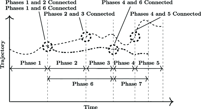
It is important to note that the event constraints of Eq.ย (3) contain functions which can relate information at the start and/or terminus of any phase (including any relationships involving any integral or static parameters), with phases not needing to be in sequential order to be linked. Moreover, it is noted that the approach to linking phases is based on well-known formulations in the literature such as those given in Ref.ย [51] and [14]. A schematic of how phases can potentially be linked is given in Fig.ย 1.

Refer to caption
Figure 1: Schematic of linkages for multiple-phase optimal control problem. The example shown in the picture consists of seven phases where the ends of phases 1, 2, and 4 are linked to the starts of phases 2, 3, and 5, respectively, while the ends of phase 1 and 6 are linked to the starts of phase 6 and 4, respectively.

3 Legendre-Gauss-Radau Collocation Method

As stated at the outset, the objective of this research is to provide researchers a computationally efficient general-purpose optimal control software for solving of a wide variety of complex constrained continuous optimal control problems using direct collocation. While in principle any collocation method can be used to approximate the optimal control problem given in Section 2, in this research the Legendre-Gauss-Radau (LGR) collocation method [23, 24, 25, 26, 40, 41, 42] is employed. It is noted that the NLP arising from the LGR collocation method has an elegant sparse structure which can be exploited as described in Refs.ย [28, 10, 52]. In addition, the LGR collocation method has a well established convergence theory as described in Refs.ย [29, 30, 31, 32, 33].

In the context of this research, a multiple-interval form of the LGR collocation method is chosen. In the multiple-interval LGR collocation method, for each phase p๐‘p of the optimal control problem (where the phase number pโˆˆ{1,โ€ฆ,P}๐‘1โ€ฆ๐‘ƒp\in\{1,\ldots,P\} has been omitted in order to improve clarity of the description of the method), the time interval tโˆˆ[t0,tf]๐‘กsubscript๐‘ก0subscript๐‘ก๐‘“t\in[t_{0},t_{f}] is converted into the domain ฯ„โˆˆ[โˆ’1,+1]๐œ11\tau\in[-1,+1] using the affine transformation,

t=tfโˆ’t02โ€‹ฯ„+tf+t02,ฯ„=2โ€‹tโˆ’t0tfโˆ’t0โˆ’1.๐‘กsubscript๐‘ก๐‘“subscript๐‘ก02๐œsubscript๐‘ก๐‘“subscript๐‘ก02๐œ2๐‘กsubscript๐‘ก0subscript๐‘ก๐‘“subscript๐‘ก01\begin{array}[]{lcl}t&=&\displaystyle\frac{t_{f}-t_{0}}{2}\tau+\frac{t_{f}+t_{0}}{2}~{},\vspace{3pt}\\ \tau&=&\displaystyle 2\frac{t-t_{0}}{t_{f}-t_{0}}-1~{}.\end{array} (9)

The domain ฯ„โˆˆ[โˆ’1,+1]๐œ11\tau\in[-1,+1] is then divided into K๐พK mesh intervals, ๐’ฎ๐“€=[๐’ฏ๐“€โˆ’1,๐’ฏ๐“€]โŠ†[โˆ’1,+1],๐“€โˆˆ{1,โ€ฆ,๐’ฆ}formulae-sequencesubscript๐’ฎ๐“€subscript๐’ฏ๐“€1subscript๐’ฏ๐“€11๐“€1โ€ฆ๐’ฆ\cal{S}_{k}=[T_{k-1},T_{k}]\subseteq[-1,+1],\;k\in\{1,\ldots,K\} such that

โ‹ƒk=1K๐’ฎ๐“€=[โˆ’1,+1],โ‹‚๐“€=1๐’ฆ๐’ฎ๐“€={๐’ฏ1,โ€ฆ,๐’ฏ๐’ฆโˆ’1},formulae-sequencesuperscriptsubscript๐‘˜1๐พsubscript๐’ฎ๐“€11superscriptsubscript๐“€1๐’ฆsubscript๐’ฎ๐“€subscript๐’ฏ1โ€ฆsubscript๐’ฏ๐’ฆ1\bigcup_{k=1}^{K}\cal{S}_{k}=[-1,+1]~{},\quad\bigcap_{k=1}^{K}\cal{S}_{k}=\{T_{1},\ldots,T_{K-1}\}~{}, (10)

and โˆ’1=T0<T1<โ€ฆ<TKโˆ’1<TK=+11subscript๐‘‡0subscript๐‘‡1โ€ฆsubscript๐‘‡๐พ1subscript๐‘‡๐พ1-1=T_{0}<T_{1}<\ldots<T_{K-1}<T_{K}=+1. For each mesh interval, the LGR points used for collocation are defined in the domain of [Tkโˆ’1,Tk]subscript๐‘‡๐‘˜1subscript๐‘‡๐‘˜[T_{k-1},T_{k}] for kโˆˆ{1,โ€ฆ,K}๐‘˜1โ€ฆ๐พk\in\{1,\ldots,K\}. The control is parameterized at the collocation points within each mesh interval. The state of the continuous optimal control problem is then approximated in mesh interval ๐’ฎ๐“€,๐“€โˆˆ{1,โ€ฆ,๐’ฆ}subscript๐’ฎ๐“€๐“€1โ€ฆ๐’ฆ\cal{S}_{k},\;k\in\{1,\ldots,K\}, as

๐ฒ(k)โ€‹(ฯ„)โ‰ˆ๐˜(k)โ€‹(ฯ„)=โˆ‘j=1Nk+1๐˜j(k)โ€‹โ„“j(k)โ€‹(ฯ„),โ„“j(k)โ€‹(ฯ„)=โˆlโ‰ jl=1Nk+1ฯ„โˆ’ฯ„l(k)ฯ„j(k)โˆ’ฯ„l(k),formulae-sequencesuperscript๐ฒ๐‘˜๐œsuperscript๐˜๐‘˜๐œsuperscriptsubscript๐‘—1subscript๐‘๐‘˜1superscriptsubscript๐˜๐‘—๐‘˜superscriptsubscriptโ„“๐‘—๐‘˜๐œsuperscriptsubscriptโ„“๐‘—๐‘˜๐œsuperscriptsubscriptproductsuperscript๐‘™๐‘—๐‘™1subscript๐‘๐‘˜1๐œsuperscriptsubscript๐œ๐‘™๐‘˜superscriptsubscript๐œ๐‘—๐‘˜superscriptsubscript๐œ๐‘™๐‘˜{\bf{y}}^{(k)}(\tau)\approx{\bf{Y}}^{(k)}(\tau)=\sum_{j=1}^{N_{k}+1}{\bf{Y}}_{j}^{(k)}\ell_{j}^{(k)}(\tau)~{},\quad\ell_{j}^{(k)}(\tau)=\prod_{\stackrel{{\scriptstyle l=1}}{{l\neq j}}}^{N_{k}+1}\frac{\tau-\tau_{l}^{(k)}}{\tau_{j}^{(k)}-\tau_{l}^{(k)}}~{}, (11)

where โ„“j(k)โ€‹(ฯ„)superscriptsubscriptโ„“๐‘—๐‘˜๐œ\ell_{j}^{(k)}(\tau) for jโˆˆ{1,โ€ฆ,Nk+1}๐‘—1โ€ฆsubscript๐‘๐‘˜1j\in\{1,\ldots,N_{k}+1\} is a basis of Lagrange polynomials, (ฯ„1(k),โ€ฆ,ฯ„Nk(k))superscriptsubscript๐œ1๐‘˜โ€ฆsuperscriptsubscript๐œsubscript๐‘๐‘˜๐‘˜\left(\tau_{1}^{(k)},\ldots,\tau_{N_{k}}^{(k)}\right) are the set of Nksubscript๐‘๐‘˜N_{k} Legendre-Gauss-Radau (LGR) [53] collocation points in the interval [Tkโˆ’1,Tk)subscript๐‘‡๐‘˜1subscript๐‘‡๐‘˜[T_{k-1},T_{k}) in ๐’ฎ๐“€subscript๐’ฎ๐“€\cal{S}_{k}, ฯ„Nk+1(k)=Tksuperscriptsubscript๐œsubscript๐‘๐‘˜1๐‘˜subscript๐‘‡๐‘˜\tau_{N_{k}+1}^{(k)}=T_{k} is a noncollocated support point, and ๐˜j(k)โ‰ก๐˜(k)โ€‹(ฯ„j(k))superscriptsubscript๐˜๐‘—๐‘˜superscript๐˜๐‘˜superscriptsubscript๐œ๐‘—๐‘˜{\bf{Y}}_{j}^{(k)}\equiv{\bf{Y}}^{(k)}(\tau_{j}^{(k)}). Differentiating ๐˜(k)โ€‹(ฯ„)superscript๐˜๐‘˜๐œ{\bf{Y}}^{(k)}(\tau) in Eq.ย (11) with respect to ฯ„๐œ\tau gives

dโ€‹๐˜(k)โ€‹(ฯ„)dโ€‹ฯ„=โˆ‘j=1Nk+1๐˜j(k)โ€‹dโ€‹โ„“j(k)โ€‹(ฯ„)dโ€‹ฯ„.๐‘‘superscript๐˜๐‘˜๐œ๐‘‘๐œsuperscriptsubscript๐‘—1subscript๐‘๐‘˜1superscriptsubscript๐˜๐‘—๐‘˜๐‘‘superscriptsubscriptโ„“๐‘—๐‘˜๐œ๐‘‘๐œ\frac{d{\bf{Y}}^{(k)}(\tau)}{d\tau}=\sum_{j=1}^{N_{k}+1}{\bf{Y}}_{j}^{(k)}\frac{d\ell_{j}^{(k)}(\tau)}{d\tau}~{}. (12)

The dynamics are then approximated at the Nksubscript๐‘๐‘˜N_{k} LGR points in mesh interval kโˆˆ{1,โ€ฆ,K}๐‘˜1โ€ฆ๐พk\in\{1,\ldots,K\} as

โˆ‘j=1Nk+1Diโ€‹j(k)โ€‹๐˜j(k)=tfโˆ’t02โ€‹๐šโ€‹(๐˜i(k),๐”i(k),tโ€‹(ฯ„i(k),t0,tf),๐ฌ),iโˆˆ{1,โ€ฆ,Nk},formulae-sequencesuperscriptsubscript๐‘—1subscript๐‘๐‘˜1superscriptsubscript๐ท๐‘–๐‘—๐‘˜superscriptsubscript๐˜๐‘—๐‘˜subscript๐‘ก๐‘“subscript๐‘ก02๐šsuperscriptsubscript๐˜๐‘–๐‘˜superscriptsubscript๐”๐‘–๐‘˜๐‘กsuperscriptsubscript๐œ๐‘–๐‘˜subscript๐‘ก0subscript๐‘ก๐‘“๐ฌ๐‘–1โ€ฆsubscript๐‘๐‘˜\sum_{j=1}^{N_{k}+1}D_{ij}^{(k)}{\bf{Y}}_{j}^{(k)}=\frac{t_{f}-t_{0}}{2}{\bf{a}}\left({\bf{Y}}_{i}^{(k)},{\bf{U}}_{i}^{(k)},t(\tau_{i}^{(k)},t_{0},t_{f}),{\bf{s}}\right)~{},\quad i\in\{1,\dots,N_{k}\}~{}, (13)

where

Diโ€‹j(k)=dโ€‹โ„“j(k)โ€‹(ฯ„i(k))dโ€‹ฯ„,iโˆˆ{1,โ€ฆ,Nk},jโˆˆ{1,โ€ฆ,Nk+1},formulae-sequencesuperscriptsubscript๐ท๐‘–๐‘—๐‘˜๐‘‘superscriptsubscriptโ„“๐‘—๐‘˜superscriptsubscript๐œ๐‘–๐‘˜๐‘‘๐œformulae-sequence๐‘–1โ€ฆsubscript๐‘๐‘˜๐‘—1โ€ฆsubscript๐‘๐‘˜1D_{ij}^{(k)}=\frac{d\ell_{j}^{(k)}(\tau_{i}^{(k)})}{d\tau}~{},\quad i\in\{1,\dots,N_{k}\}~{},~{}j\in\{1,\dots,N_{k}+1\}~{},

are the elements of the Nkร—(Nk+1)subscript๐‘๐‘˜subscript๐‘๐‘˜1N_{k}\times(N_{k}+1) Legendre-Gauss-Radau differentiation matrix [23] in mesh interval ๐’ฎ๐“€subscript๐’ฎ๐“€\cal{S}_{k}, kโˆˆ{1,โ€ฆ,K}๐‘˜1โ€ฆ๐พ\;k\in\{1,\ldots,K\}, and ๐”i(k)superscriptsubscript๐”๐‘–๐‘˜{\bf{U}}_{i}^{(k)} is the parameterized control at the itโ€‹hsuperscript๐‘–๐‘กโ„Ži^{th} collocation point in mesh interval k๐‘˜k. Finally, reintroducing the phase notation pโˆˆ{1,โ€ฆ,P}๐‘1โ€ฆ๐‘ƒp\in\{1,\ldots,P\}, the phases of the problem are linked together by the event constraints

๐›minโ‰ค๐›โ€‹(๐„(1),โ€ฆ,๐„(P),๐ฌ)โ‰ค๐›max,subscript๐›๐›superscript๐„1โ€ฆsuperscript๐„๐‘ƒ๐ฌsubscript๐›{\bf{b}}_{\min}\leq{\bf{b}}\left({\bf{E}}^{(1)},\dots,{\bf{E}}^{(P)},{\bf{s}}\right)\leq{\bf{b}}_{\max}~{}, (14)

where ๐„(p)superscript๐„๐‘{\bf{E}}^{(p)} is the endpoint approximation vector for phase p๐‘p defined as

๐„(p)=[๐˜1(p),t0(p),๐˜N(p)+1(p),tf(p),๐(p)],superscript๐„๐‘superscriptsubscript๐˜1๐‘superscriptsubscript๐‘ก0๐‘superscriptsubscript๐˜superscript๐‘๐‘1๐‘superscriptsubscript๐‘ก๐‘“๐‘superscript๐๐‘{\bf{E}}^{(p)}=\left[{\bf{Y}}_{1}^{(p)},t_{0}^{(p)},{\bf{Y}}_{N^{(p)}+1}^{(p)},t_{f}^{(p)},{\bf{Q}}^{(p)}\right]~{}, (15)

such that N(p)superscript๐‘๐‘N^{(p)} is the total number of collocation points used in phase p๐‘p given by,

N(p)=โˆ‘k=1K(p)Nk(p),superscript๐‘๐‘superscriptsubscript๐‘˜1superscript๐พ๐‘superscriptsubscript๐‘๐‘˜๐‘N^{(p)}=\sum_{k=1}^{K^{(p)}}N_{k}^{(p)}~{}, (16)

and ๐(p)โˆˆโ„1ร—nq(p)superscript๐๐‘superscriptโ„1superscriptsubscript๐‘›๐‘ž๐‘{\bf{Q}}^{(p)}\in\mathbb{R}^{1~{}\times~{}n_{q}^{(p)}} is the integral approximation vector in phase p๐‘p.

The aforementioned LGR discretization then leads to the following NLP. Minimize the objective function

๐’ฅ=ฯ•โ€‹(๐„(1),โ€ฆ,๐„(๐’ซ),๐ฌ),๐’ฅitalic-ฯ•superscript๐„1โ€ฆsuperscript๐„๐’ซ๐ฌ\cal{J}=\cal{\phi}\left({\bf{E}}^{(1)},\dots,{\bf{E}}^{(P)},{\bf{s}}\right)~{}, (17)

subject to the defect constraints

๐šซ(p)=๐ƒ(p)โ€‹๐˜(p)โˆ’tf(p)โˆ’t0(p)2โ€‹๐€(p)=๐ŸŽ,pโˆˆ{1,โ€ฆ,P},formulae-sequencesuperscript๐šซ๐‘superscript๐ƒ๐‘superscript๐˜๐‘superscriptsubscript๐‘ก๐‘“๐‘superscriptsubscript๐‘ก0๐‘2superscript๐€๐‘0๐‘1โ€ฆ๐‘ƒ{\bf{\Delta}}^{(p)}={\bf{D}}^{(p)}{\bf{Y}}^{(p)}-\frac{t_{f}^{(p)}-t_{0}^{(p)}}{2}{\bf{A}}^{(p)}={\bf{0}}~{},\quad p\in\{1,\dots,P\}~{}, (18)

the path constraints

๐œmin(p)โ‰ค๐‚i(p)โ‰ค๐œmax(p),iโˆˆ{1,โ€ฆ,N(p)},pโˆˆ{1,โ€ฆ,P},formulae-sequencesuperscriptsubscript๐œ๐‘superscriptsubscript๐‚๐‘–๐‘superscriptsubscript๐œ๐‘formulae-sequence๐‘–1โ€ฆsuperscript๐‘๐‘๐‘1โ€ฆ๐‘ƒ{\bf{c}}_{\min}^{(p)}\leq{\bf{C}}_{i}^{(p)}\leq{\bf{c}}_{\max}^{(p)}~{},\quad i\in\{1,\dots,N^{(p)}\},p\in\{1,\dots,P\}~{}, (19)

the event constraints

๐›minโ‰ค๐›โ€‹(๐„(1),โ€ฆ,๐„(P),๐ฌ)โ‰ค๐›max,subscript๐›๐›superscript๐„1โ€ฆsuperscript๐„๐‘ƒ๐ฌsubscript๐›{\bf{b}}_{\min}\leq{\bf{b}}\left({\bf{E}}^{(1)},\dots,{\bf{E}}^{(P)},{\bf{s}}\right)\leq{\bf{b}}_{\max}~{}, (20)

the integral constraints

๐ชmin(p)โ‰ค๐(p)โ‰ค๐ชmax(p),pโˆˆ{1,โ€ฆ,P},formulae-sequencesuperscriptsubscript๐ช๐‘superscript๐๐‘superscriptsubscript๐ช๐‘๐‘1โ€ฆ๐‘ƒ{\bf{q}}_{\min}^{(p)}\leq{\bf{Q}}^{(p)}\leq{\bf{q}}_{\max}^{(p)}~{},\quad p\in\{1,\dots,P\}~{}, (21)

the static parameter constraints

๐ฌminโ‰ค๐ฌโ‰ค๐ฌmax,subscript๐ฌ๐ฌsubscript๐ฌ{\bf{s}}_{\min}\leq{\bf{s}}\leq{\bf{s}}_{\max}~{}, (22)

and integral approximation constraints

๐†(p)=๐(p)โˆ’tf(p)โˆ’t0(p)2โ€‹[๐ฐ(p)]๐–ณโ€‹๐†(p)=๐ŸŽ,pโˆˆ{1,โ€ฆ,P},formulae-sequencesuperscript๐†๐‘superscript๐๐‘superscriptsubscript๐‘ก๐‘“๐‘superscriptsubscript๐‘ก0๐‘2superscriptmatrixsuperscript๐ฐ๐‘๐–ณsuperscript๐†๐‘0๐‘1โ€ฆ๐‘ƒ\boldsymbol{\rho}^{(p)}={\bf{Q}}^{(p)}-\frac{t_{f}^{(p)}-t_{0}^{(p)}}{2}\begin{bmatrix}{\bf{w}}^{(p)}\end{bmatrix}^{{}^{\sf T}}{\bf{G}}^{(p)}={\bf{0}}~{},\quad p\in\{1,\dots,P\}~{}, (23)

where

๐€(p)=[๐š(p)โ€‹(๐˜1(p),๐”1(p),t1(p),๐ฌ)โ‹ฎ๐š(p)โ€‹(๐˜N(p)(p),๐”N(p)(p),tN(p)(p),๐ฌ)]โˆˆโ„N(p)ร—ny(p),superscript๐€๐‘matrixsuperscript๐š๐‘superscriptsubscript๐˜1๐‘superscriptsubscript๐”1๐‘superscriptsubscript๐‘ก1๐‘๐ฌโ‹ฎsuperscript๐š๐‘superscriptsubscript๐˜superscript๐‘๐‘๐‘superscriptsubscript๐”superscript๐‘๐‘๐‘superscriptsubscript๐‘กsuperscript๐‘๐‘๐‘๐ฌsuperscriptโ„superscript๐‘๐‘superscriptsubscript๐‘›๐‘ฆ๐‘{\bf{A}}^{(p)}=\begin{bmatrix}{\bf{a}}^{(p)}\left({\bf{Y}}_{1}^{(p)},{\bf{U}}_{1}^{(p)},t_{1}^{(p)},{\bf{s}}\right)\\ \vdots\\ {\bf{a}}^{(p)}\left({\bf{Y}}_{N^{(p)}}^{(p)},{\bf{U}}_{N^{(p)}}^{(p)},t_{N^{(p)}}^{(p)},{\bf{s}}\right)\end{bmatrix}\in\mathbb{R}^{N^{(p)}~{}\times~{}n_{y}^{(p)}}~{}, (24)
๐‚(p)=[๐œ(p)โ€‹(๐˜1(p),๐”1(p),t1(p),๐ฌ)โ‹ฎ๐œ(p)โ€‹(๐˜N(p)(p),๐”N(p)(p),tN(p)(p),๐ฌ)]โˆˆโ„N(p)ร—nc(p),superscript๐‚๐‘matrixsuperscript๐œ๐‘superscriptsubscript๐˜1๐‘superscriptsubscript๐”1๐‘superscriptsubscript๐‘ก1๐‘๐ฌโ‹ฎsuperscript๐œ๐‘superscriptsubscript๐˜superscript๐‘๐‘๐‘superscriptsubscript๐”superscript๐‘๐‘๐‘superscriptsubscript๐‘กsuperscript๐‘๐‘๐‘๐ฌsuperscriptโ„superscript๐‘๐‘superscriptsubscript๐‘›๐‘๐‘{\bf{C}}^{(p)}=\begin{bmatrix}{\bf{c}}^{(p)}\left({\bf{Y}}_{1}^{(p)},{\bf{U}}_{1}^{(p)},t_{1}^{(p)},{\bf{s}}\right)\\ \vdots\\ {\bf{c}}^{(p)}\left({\bf{Y}}_{N^{(p)}}^{(p)},{\bf{U}}_{N^{(p)}}^{(p)},t_{N^{(p)}}^{(p)},{\bf{s}}\right)\end{bmatrix}\in\mathbb{R}^{N^{(p)}~{}\times~{}n_{c}^{(p)}}~{}, (25)
๐†(p)=[๐ (p)โ€‹(๐˜1(p),๐”1(p),t1(p),๐ฌ)โ‹ฎ๐ (p)โ€‹(๐˜N(p)(p),๐”N(p)(p),tN(p)(p),๐ฌ)]โˆˆโ„N(p)ร—nq(p),superscript๐†๐‘matrixsuperscript๐ ๐‘superscriptsubscript๐˜1๐‘superscriptsubscript๐”1๐‘superscriptsubscript๐‘ก1๐‘๐ฌโ‹ฎsuperscript๐ ๐‘superscriptsubscript๐˜superscript๐‘๐‘๐‘superscriptsubscript๐”superscript๐‘๐‘๐‘superscriptsubscript๐‘กsuperscript๐‘๐‘๐‘๐ฌsuperscriptโ„superscript๐‘๐‘superscriptsubscript๐‘›๐‘ž๐‘{\bf{G}}^{(p)}=\begin{bmatrix}{\bf{g}}^{(p)}\left({\bf{Y}}_{1}^{(p)},{\bf{U}}_{1}^{(p)},t_{1}^{(p)},{\bf{s}}\right)\\ \vdots\\ {\bf{g}}^{(p)}\left({\bf{Y}}_{N^{(p)}}^{(p)},{\bf{U}}_{N^{(p)}}^{(p)},t_{N^{(p)}}^{(p)},{\bf{s}}\right)\end{bmatrix}\in\mathbb{R}^{N^{(p)}~{}\times~{}n_{q}^{(p)}}~{}, (26)

๐ƒ(p)โˆˆโ„N(p)ร—[N(p)+1]superscript๐ƒ๐‘superscriptโ„superscript๐‘๐‘delimited-[]superscript๐‘๐‘1{\bf{D}}^{(p)}\in\mathbb{R}^{N^{(p)}~{}\times~{}[N^{(p)}+1]} is the LGR differentiation matrix in phase pโˆˆ{1,โ€ฆ,P}๐‘1โ€ฆ๐‘ƒp\in\{1,\ldots,P\}, and ๐ฐ(p)โˆˆโ„N(p)ร—1superscript๐ฐ๐‘superscriptโ„superscript๐‘๐‘1{\bf{w}}^{(p)}\in\mathbb{R}^{N^{(p)}~{}\times~{}1} are the LGR weights at each node in phase p๐‘p. It is noted that ๐š(p)โˆˆโ„1ร—ny(p)superscript๐š๐‘superscriptโ„1superscriptsubscript๐‘›๐‘ฆ๐‘{\bf{a}}^{(p)}\in\mathbb{R}^{1~{}\times~{}n_{y}^{(p)}}, ๐œ(p)โˆˆโ„1ร—nc(p)superscript๐œ๐‘superscriptโ„1superscriptsubscript๐‘›๐‘๐‘{\bf{c}}^{(p)}\in\mathbb{R}^{1~{}\times~{}n_{c}^{(p)}}, and ๐ (p)โˆˆโ„1ร—nq(p)superscript๐ ๐‘superscriptโ„1superscriptsubscript๐‘›๐‘ž๐‘{\bf{g}}^{(p)}\in\mathbb{R}^{1~{}\times~{}n_{q}^{(p)}} correspond, respectively, to the functions that define the right-hand side of the dynamics, the path constraints, and the integrands in phase pโˆˆ{1,โ€ฆ,P}๐‘1โ€ฆ๐‘ƒp\in\{1,\ldots,P\}, where ny(p)superscriptsubscript๐‘›๐‘ฆ๐‘n_{y}^{(p)}, nc(p)superscriptsubscript๐‘›๐‘๐‘n_{c}^{(p)}, and nq(p)superscriptsubscript๐‘›๐‘ž๐‘n_{q}^{(p)} are, respectively, the number of state components, path constraints, and integral components in phase p๐‘p. Finally, the state matrix, ๐˜(p)โˆˆโ„[N(p)+1]ร—ny(p)superscript๐˜๐‘superscriptโ„delimited-[]superscript๐‘๐‘1superscriptsubscript๐‘›๐‘ฆ๐‘{\bf{Y}}^{(p)}\in\mathbb{R}^{[N^{(p)}+1]~{}\times~{}n_{y}^{(p)}}, and the control matrix, ๐”(p)โˆˆโ„N(p)ร—nu(p)superscript๐”๐‘superscriptโ„superscript๐‘๐‘superscriptsubscript๐‘›๐‘ข๐‘{\bf{U}}^{(p)}\in\mathbb{R}^{N^{(p)}~{}\times~{}n_{u}^{(p)}}, in phase pโˆˆ{1,โ€ฆ,P}๐‘1โ€ฆ๐‘ƒp\in\{1,\ldots,P\} are formed as

๐˜(p)=[๐˜1(p)โ‹ฎ๐˜N(p)+1(p)]โ€‹ย andย โ€‹๐”(p)=[๐”1(p)โ‹ฎ๐”N(p)(p)],superscript๐˜๐‘matrixsubscriptsuperscript๐˜๐‘1โ‹ฎsubscriptsuperscript๐˜๐‘superscript๐‘๐‘1ย andย superscript๐”๐‘matrixsubscriptsuperscript๐”๐‘1โ‹ฎsubscriptsuperscript๐”๐‘superscript๐‘๐‘{\bf{Y}}^{(p)}=\begin{bmatrix}{\bf{Y}}^{(p)}_{1}\\ \vdots\\ {\bf{Y}}^{(p)}_{N^{(p)}+1}\end{bmatrix}\text{ and }{\bf{U}}^{(p)}=\begin{bmatrix}{\bf{U}}^{(p)}_{1}\\ \vdots\\ {\bf{U}}^{(p)}_{N^{(p)}}\end{bmatrix}~{}, (27)

respectively, where nu(p)superscriptsubscript๐‘›๐‘ข๐‘n_{u}^{(p)} is the number of control components in phase p๐‘p.

4 Major Components of โ„‚โ€‹๐”พโ€‹โ„™โ€‹๐•†โ€‹โ„™โ€‹๐•Šโ„‚๐”พโ„™๐•†โ„™๐•Š\mathbb{CGPOPS}

In this section we describe the major components of the C++ software โ„‚โ€‹๐”พโ€‹โ„™โ€‹๐•†โ€‹โ„™โ€‹๐•Šโ„‚๐”พโ„™๐•†โ„™๐•Š{\mathbb{CGPOPS}} that implements the aforementioned LGR collocation method. In Section 4.1, the large sparse nonlinear programming problem (NLP) associated with the LGR collocation method is described. In Section 4.2, the structure of the NLP described in Section 4.1 is shown. In Section 4.3 the method for scaling the NLP via scaling of the optimal control problem is over-viewed. In Section 4.4, the approach for estimating the derivatives required by the NLP solver is explained. In Section 4.5, the method for determining the dependencies of each optimal control function in order to provide the most sparse NLP to the NLP solver is presented. In Section 4.6 the hโ€‹pโ„Ž๐‘hp mesh refinement methods that are included in the software in order to iteratively determine a mesh that satisfies a user-specified accuracy tolerance are described. Finally, in Section 4.7 we provide a high level description of the algorithmic flow of โ„‚โ€‹๐”พโ€‹โ„™โ€‹๐•†โ€‹โ„™โ€‹๐•Šโ„‚๐”พโ„™๐•†โ„™๐•Š{\mathbb{CGPOPS}}.

4.1 Sparse NLP Arising from Radau Collocation Method

The resulting nonlinear programming problem (NLP) that arises when using LGR collocation to discretize the continuous optimal control problem is given as follows. Determine the NLP decision vector, ๐ณ๐ณ{\bf{z}}, that minimizes the NLP objective function,

fโ€‹(๐ณ),๐‘“๐ณf({\bf{z}})~{}, (28)

subject to the constraints

๐‡minโ‰ค๐‡โ€‹(๐ณ)โ‰ค๐‡max,subscript๐‡๐‡๐ณsubscript๐‡{\bf{H}}_{\min}\leq{\bf{H}}({\bf{z}})\leq{\bf{H}}_{\max}~{}, (29)

and the variable bounds

๐ณminโ‰ค๐ณโ‰ค๐ณmax.subscript๐ณ๐ณsubscript๐ณ{\bf{z}}_{\min}\leq{\bf{z}}\leq{\bf{z}}_{\max}~{}. (30)

It is noted that, while the size of the NLP arising from the LGR collocation method changes depending upon the number of mesh intervals and LGR points used in each phase, the structure of the NLP remains the same regardless of the size of the NLP. Finally, in the sections that follow, the subscript ":::" denotes either a row or a column, where the โ€œ:::โ€ notation is analogous to the syntax used in the MATLAB programming language.

4.1.1 NLP Variables

For a continuous optimal control problem transcribed into P๐‘ƒP phases, the NLP decision vector, ๐ณ๐ณ{\bf{z}}, has the following form:

๐ณ=[๐ณ(1)โ‹ฎ๐ณ(P)s1โ‹ฎsns],whereย โ€‹๐ณ(p)=[๐˜(:,1)(p)โ‹ฎ๐˜(:,ny(p))(p)๐”(:,1)(p)โ‹ฎ๐”(:,nu(p))(p)(๐(p))๐–ณt0(p)tf(p)],formulae-sequence๐ณmatrixsuperscript๐ณ1โ‹ฎsuperscript๐ณ๐‘ƒsubscript๐‘ 1โ‹ฎsubscript๐‘ subscript๐‘›๐‘ whereย superscript๐ณ๐‘matrixsuperscriptsubscript๐˜:1๐‘โ‹ฎsuperscriptsubscript๐˜:superscriptsubscript๐‘›๐‘ฆ๐‘๐‘superscriptsubscript๐”:1๐‘โ‹ฎsuperscriptsubscript๐”:superscriptsubscript๐‘›๐‘ข๐‘๐‘superscriptsuperscript๐๐‘๐–ณsuperscriptsubscript๐‘ก0๐‘superscriptsubscript๐‘ก๐‘“๐‘{\bf{z}}=\begin{bmatrix}{\bf{z}}^{(1)}\\ \vdots\\ {\bf{z}}^{(P)}\\ s_{1}\\ \vdots\\ s_{n_{s}}\end{bmatrix}~{},\quad\text{where }{\bf{z}}^{(p)}=\begin{bmatrix}{\bf{Y}}_{(:,1)}^{(p)}\\ \vdots\\ {\bf{Y}}_{(:,n_{y}^{(p)})}^{(p)}\vspace{3pt}\\ {\bf{U}}_{(:,1)}^{(p)}\\ \vdots\\ {\bf{U}}_{(:,n_{u}^{(p)})}^{(p)}\vspace{3pt}\\ ({\bf{Q}}^{(p)})^{{}^{\sf T}}\\ t_{0}^{(p)}\\ t_{f}^{(p)}\\ \end{bmatrix}~{}, (31)

๐˜(p)โˆˆโ„N(p)ร—ny(p)superscript๐˜๐‘superscriptโ„superscript๐‘๐‘superscriptsubscript๐‘›๐‘ฆ๐‘{\bf{Y}}^{(p)}\in\mathbb{R}^{N^{(p)}~{}\times~{}n_{y}^{(p)}} is the state approximation matrix [see Eq.ย (27)], ๐”(p)โˆˆโ„N(p)ร—nu(p)superscript๐”๐‘superscriptโ„superscript๐‘๐‘superscriptsubscript๐‘›๐‘ข๐‘{\bf{U}}^{(p)}\in\mathbb{R}^{N^{(p)}~{}\times~{}n_{u}^{(p)}} is the control parameterization matrix [see Eq.ย (27)], ๐(p)โˆˆโ„1ร—nq(p)superscript๐๐‘superscriptโ„1superscriptsubscript๐‘›๐‘ž๐‘{\bf{Q}}^{(p)}\in\mathbb{R}^{1~{}\times~{}n_{q}^{(p)}} is the integral approximation vector, and t0(p)superscriptsubscript๐‘ก0๐‘t_{0}^{(p)} and tf(p)superscriptsubscript๐‘ก๐‘“๐‘t_{f}^{(p)} are scalars of the initial and final time, respectively, for phase pโˆˆ{1,โ€ฆ,P}๐‘1โ€ฆ๐‘ƒp\in\{1,\ldots,P\}, and sisubscript๐‘ ๐‘–s_{i} for iโˆˆ{1,โ€ฆ,ns}๐‘–1โ€ฆsubscript๐‘›๐‘ i\in\{1,\dots,n_{s}\} are the static parameters appearing throughout the entire problem.

4.1.2 NLP Objective and Constraint Functions

The NLP objective function, fโ€‹(๐ณ)๐‘“๐ณf({\bf{z}}), is given in the form

fโ€‹(๐ณ)=ฯ•(p)โ€‹(๐„(1),โ€ฆ,๐„(P),๐ฌ),๐‘“๐ณsuperscriptitalic-ฯ•๐‘superscript๐„1โ€ฆsuperscript๐„๐‘ƒ๐ฌf({\bf{z}})=\phi^{(p)}({\bf{E}}^{(1)},\ldots,{\bf{E}}^{(P)},{\bf{s}})~{}, (32)

where ๐„(p),pโˆˆ{1,โ€ฆ,P}superscript๐„๐‘๐‘1โ€ฆ๐‘ƒ{\bf{E}}^{(p)},~{}p\in\{1,\ldots,P\}, is the endpoint approximation vector defined in Eq. (15), and the typical cost functional of a general multiple-phase optimal control problem has been turned simply into a Mayer cost function by using the integral variables, ๐(p)superscript๐๐‘{\bf{Q}}^{(p)}, to approximate the Lagrange cost in each phaseย p๐‘p. The NLP constraint vector, ๐‡โ€‹(๐ณ)๐‡๐ณ{\bf{H}}({\bf{z}}), is given in the form

๐‡โ€‹(๐ณ)=[๐ก(1)โ‹ฎ๐ก(P)๐›],whereย โ€‹๐ก(p)=[๐šซ(:,1)(p)โ‹ฎ๐šซ(:,ny(p))(p)๐‚(:,1)(p)โ‹ฎ๐‚(:,nc(p))(p)(๐†(p))๐–ณ],p={1,โ€ฆ,P},formulae-sequence๐‡๐ณmatrixsuperscript๐ก1โ‹ฎsuperscript๐ก๐‘ƒ๐›formulae-sequencewhereย superscript๐ก๐‘matrixsuperscriptsubscript๐šซ:1๐‘โ‹ฎsuperscriptsubscript๐šซ:superscriptsubscript๐‘›๐‘ฆ๐‘๐‘superscriptsubscript๐‚:1๐‘โ‹ฎsuperscriptsubscript๐‚:superscriptsubscript๐‘›๐‘๐‘๐‘superscriptsuperscript๐†๐‘๐–ณ๐‘1โ€ฆ๐‘ƒ{\bf{H}}({\bf{z}})=\begin{bmatrix}{\bf{h}}^{(1)}\\ \vdots\\ {\bf{h}}^{(P)}\\ {\bf{b}}\end{bmatrix}~{},~{}\text{where }{\bf{h}}^{(p)}=\begin{bmatrix}{\bf{\Delta}}_{(:,1)}^{(p)}\\ \vdots\\ {\bf{\Delta}}_{(:,n_{y}^{(p)})}^{(p)}\vspace{3pt}\\ {\bf{C}}_{(:,1)}^{(p)}\\ \vdots\\ {\bf{C}}_{(:,n_{c}^{(p)})}^{(p)}\\ (\boldsymbol{\rho}^{(p)})^{{}^{\sf T}}\\ \end{bmatrix}~{},\quad p=\{1,\dots,P\}~{}, (33)

๐šซ(p)โˆˆโ„N(p)ร—ny(p)superscript๐šซ๐‘superscriptโ„superscript๐‘๐‘superscriptsubscript๐‘›๐‘ฆ๐‘{\bf{\Delta}}^{(p)}\in\mathbb{R}^{N^{(p)}~{}\times~{}n_{y}^{(p)}}, ๐†(p)โˆˆโ„1ร—nq(p)superscript๐†๐‘superscriptโ„1superscriptsubscript๐‘›๐‘ž๐‘\boldsymbol{\rho}^{(p)}\in\mathbb{R}^{1~{}\times~{}n_{q}^{(p)}}, and ๐‚(p)โˆˆโ„N(p)ร—nc(p)superscript๐‚๐‘superscriptโ„superscript๐‘๐‘superscriptsubscript๐‘›๐‘๐‘{\bf{C}}^{(p)}\in\mathbb{R}^{N^{(p)}~{}\times~{}n_{c}^{(p)}}, are, respectively, the defect constraint matrix, the integral approximation constraint vector, and the path constraint matrix in phase pโˆˆ{1,โ€ฆ,P}๐‘1โ€ฆ๐‘ƒp\in\{1,\dots,P\}, and ๐›โˆˆโ„nbร—1๐›superscriptโ„subscript๐‘›๐‘1{\bf{b}}\in\mathbb{R}^{n_{b}~{}\times~{}1} is the event constraint vector for the entire problem. The defect constraint matrix, integral approximation constraint vector, and path constraint matrix in phase p๐‘p are defined by Eqs.ย (18), (23), and (25), respectively. It is noted that the constraints are divided into the equality defect and integral constraints

๐šซ(p)=๐ŸŽ,๐†(p)=๐ŸŽ,pโˆˆ{1,โ€ฆ,P},superscript๐šซ๐‘0superscript๐†๐‘0๐‘1โ€ฆ๐‘ƒ\begin{array}[]{rcl}\boldsymbol{\Delta}^{(p)}&=&{\bf{0}}~{},\\ \boldsymbol{\rho}^{(p)}&=&{\bf{0}}~{},\end{array}\quad p\in\{1,\dots,P\}~{}, (34)

and the inequality discretized path and event constraints

๐œmin(p)โ‰ค๐‚i(p)โ‰ค๐œmax(p),iโˆˆ{1,โ€ฆ,nc(p)},pโˆˆ{1,โ€ฆ,P},๐›minโ‰ค๐›โ‰ค๐›max.subscriptsuperscript๐œ๐‘superscriptsubscript๐‚๐‘–๐‘subscriptsuperscript๐œ๐‘formulae-sequence๐‘–1โ€ฆsuperscriptsubscript๐‘›๐‘๐‘๐‘1โ€ฆ๐‘ƒsubscript๐›๐›subscript๐›missing-subexpression\begin{array}[]{rcccll}{\bf{c}}^{(p)}_{\min}&\leq&{\bf{C}}_{i}^{(p)}&\leq&{\bf{c}}^{(p)}_{\max}~{},&i\in\{1,\dots,n_{c}^{(p)}\}~{},~{}p\in\{1,\dots,P\}~{},\\ {\bf{b}}_{\min}&\leq&{\bf{b}}&\leq&{\bf{b}}_{\max}~{}.\end{array} (35)

4.2 Sparse Structure of NLP Derivative Functions

The structure of the NLP created by the LGR collocation method has been described in detail in Refs.ย [28] and [52]. Specifically, Refs.ย [28] and [52] describe the sparse structure of the NLP for the differential form of the LGR collocation method for the single and multiple phase optimal control problem, respectively. As described in Sectionย 4.1.1, the values of the state approximation coefficients at the discretization points, the control parameters at the collocation points, the initial time, the final time, and the integral vector of each phase, as well as any static parameters of the problem make up the NLP decision vector. The NLP constraints vector consists of the defect constraints and path constraints applied at each of the collocation points, as well as any integral approximation constraints, for each phase, and event constraints, as described in Sectionย 4.1.2. The derivation of the NLP derivative matrices in terms of the original continuous optimal control problem functions is described in detail in Refs.ย [28, 10, 52] and is beyond the scope of this paper. It is noted that the sparsity exploitation derived in Refs.ย [28, 10, 52] requires computing partial derivatives of the continuous optimal control problem functions on the first- and second-order derivative levels.

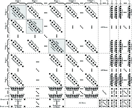
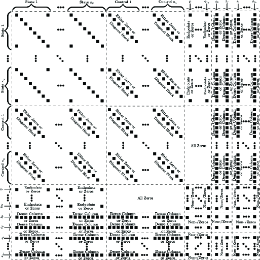
Examples of the sparsity patterns of the NLP constraint Jacobian and Lagrangian Hessian are shown, respectively, in Figs.ย 2a and 2b for a single-phase optimal control problem. It is noted that for the NLP constraint Jacobian, all of the off-diagonal phase blocks relating constraints in phase i๐‘–i to variables in phase j๐‘—j for iโ‰ j๐‘–๐‘—i\neq j are all zeros. Similarly, for the NLP Lagrangian Hessian, all of the off-diagonal phase blocks relating variables in phase i๐‘–i to variables in phase j๐‘—j for iโ‰ j๐‘–๐‘—i\neq j are all zeros except for the variables making up the endpoint vectors which may be related via the objective function or event constraints. The sparsity patterns shown in Fig.ย 2 are determined explicitly by identifying the derivative dependencies of the NLP objective and constraints functions with respect to the NLP decision vector variables. It is noted that the phases are connected using the initial and terminal values of the time and state in each phase along with the static parameters.
Refer to caption
(a) NLP Constraint Jacobian
Refer to caption
(b) NLP Lagrangian Hessian
Figure 2: Example Sparsity Patterns for Single Phase Optimal Control Problem Containing nysubscript๐‘›๐‘ฆn_{y} State Components, nusubscript๐‘›๐‘ขn_{u} Control Components, nqsubscript๐‘›๐‘žn_{q} Integral Components, and ncsubscript๐‘›๐‘n_{c} Path Constraints, nssubscript๐‘›๐‘ n_{s} Static Parameters, and nbsubscript๐‘›๐‘n_{b} Event Constraints.

4.3 Scaling of Optimal Control Problem for NLP

The NLP described in Sectionย 4.1 must be well scaled in order for the NLP solver to obtain a solution. โ„‚โ€‹๐”พโ€‹โ„™โ€‹๐•†โ€‹โ„™โ€‹๐•Šโ„‚๐”พโ„™๐•†โ„™๐•Š{\mathbb{CGPOPS}} includes the option for the NLP to be scaled automatically by scaling the continuous optimal control problem. The approach to automatic scaling is to scale the variables and the first derivatives of the optimal control functions to be โ‰ˆ๐’ชโ€‹(1)absent๐’ช1\approx{\cal{O}}(1). First, the optimal control variables are scaled to lie on the unit interval [โˆ’1/2,1/2]1212[-1/2,1/2] and is accomplished as follows. Suppose it is desired to scale an arbitrary variable xโˆˆ[a,b]๐‘ฅ๐‘Ž๐‘x\in[a,b] to x~~๐‘ฅ\tilde{x} such that x~โˆˆ[โˆ’1/2,1/2]~๐‘ฅ1212\tilde{x}\in[-1/2,1/2]. This variable scaling is accomplished via the affine transformation

x~=vxโ€‹x+rx,~๐‘ฅsubscript๐‘ฃ๐‘ฅ๐‘ฅsubscript๐‘Ÿ๐‘ฅ\tilde{x}=v_{x}x+r_{x}, (36)

where vxsubscript๐‘ฃ๐‘ฅv_{x} and rxsubscript๐‘Ÿ๐‘ฅr_{x} are the variable scale and shift, respectively, defined as

vx=1bโˆ’a,rx=12โˆ’bbโˆ’a.subscript๐‘ฃ๐‘ฅ1๐‘๐‘Žsubscript๐‘Ÿ๐‘ฅ12๐‘๐‘๐‘Ž\begin{array}[]{rcl}v_{x}&=&\displaystyle\frac{1}{b-a}~{},\\ r_{x}&=&\displaystyle\frac{1}{2}-\frac{b}{b-a}~{}.\end{array} (37)

Every variable in the continuous optimal control problem is scaled using Eqs.ย (36) and (37). Next, the Jacobian of the NLP constraints can be made โ‰ˆ๐’ชโ€‹(1)absent๐’ช1\approx{\cal{O}}(1) by scaling the derivatives of the optimal control functions to be approximately unity. First, using the approach derived in [14], in โ„‚โ€‹๐”พโ€‹โ„™โ€‹๐•†โ€‹โ„™โ€‹๐•Šโ„‚๐”พโ„™๐•†โ„™๐•Š{\mathbb{CGPOPS}} the defect constraints are scaled using the same scale factors as were used to scale the state. Next, the objective function, event constraints, and path constraints scale factors are obtained by sampling the gradient of each constraint at a variety of sample points within the bounds of the unscaled optimal control problem and taking the average norm of each gradient across all sample points.

4.4 Computation Derivatives of NLP Functions

The NLP derivative functions are obtained by exploiting the sparse structure of the NLP arising from the hโ€‹pโ„Ž๐‘hp LGR collocation method. Specifically, in Refs.ย [28, 52] it has been shown that by using the derivative form of the LGR collocation method, the NLP derivatives can be obtained by computing the derivatives of the optimal control problem functions at the LGR points and inserting these derivatives into the appropriate locations in the NLP derivative functions. In โ„‚โ€‹๐”พโ€‹โ„™โ€‹๐•†โ€‹โ„™โ€‹๐•Šโ„‚๐”พโ„™๐•†โ„™๐•Š{\mathbb{CGPOPS}}, the optimal control derivative functions are approximated using one of four types of derivative estimation methods: sparse central finite-differencing, bicomplex-step derivative approximations, hyper-dual derivative approximations, and automatic differentiation.

4.4.1 Central Finite Difference

To see how the central finite-difference derivative approximation works in practice, consider the function ๐Ÿโ€‹(๐ฑ)๐Ÿ๐ฑ{\bf{f}}({\bf{x}}), where ๐Ÿ:โ„nโ†’โ„m:๐Ÿโ†’superscriptโ„๐‘›superscriptโ„๐‘š{\bf{f}}:\mathbb{R}^{n}\rightarrow\mathbb{R}^{m} is one of the optimal control functions (that is, n๐‘›n and m๐‘šm are, respectively, the size of an optimal control variable and an optimal control function). Then โˆ‚๐Ÿ/โˆ‚๐ฑ๐Ÿ๐ฑ\partial{\bf{f}}/\partial{\bf{x}} is approximated using a central finite difference as

โˆ‚๐Ÿโˆ‚xiโ‰ˆ๐Ÿโ€‹(๐ฑ+๐กi)โˆ’๐Ÿโ€‹(๐ฑโˆ’๐กi)2โ€‹h,๐Ÿsubscript๐‘ฅ๐‘–๐Ÿ๐ฑsubscript๐ก๐‘–๐Ÿ๐ฑsubscript๐ก๐‘–2โ„Ž\frac{\partial{\bf{f}}}{\partial x_{i}}\approx\frac{{\bf{f}}({\bf{x}}+{\bf{h}}_{i})-{\bf{f}}({\bf{x}}-{\bf{h}}_{i})}{2h}, (38)

where ๐กisubscript๐ก๐‘–{\bf{h}}_{i} arises from perturbing the itโ€‹hsuperscript๐‘–๐‘กโ„Ži^{th} component of ๐ฑ๐ฑ{\bf{x}}. The vector ๐กisubscript๐ก๐‘–{\bf{h}}_{i} is computed as

๐กi=hiโ€‹๐žisubscript๐ก๐‘–subscriptโ„Ž๐‘–subscript๐ž๐‘–{\bf{h}}_{i}=h_{i}{\bf{e}}_{i} (39)

where ๐žisubscript๐ž๐‘–{\bf{e}}_{i} is the itโ€‹hsuperscript๐‘–๐‘กโ„Ži^{th} row of the nร—n๐‘›๐‘›n\times n identity matrix and hisubscriptโ„Ž๐‘–h_{i} is the perturbation size associated with xisubscript๐‘ฅ๐‘–x_{i}. The perturbation hisubscriptโ„Ž๐‘–h_{i} is computed using the equation

hi=hโ€‹(1+|xi|),subscriptโ„Ž๐‘–โ„Ž1subscript๐‘ฅ๐‘–h_{i}=h(1+|x_{i}|), (40)

where the base perturbation size hโ„Žh is chosen to be the optimal step size for a function whose input and output are โ‰ˆ๐’ชโ€‹(1)absent๐’ช1\approx{\cal{O}}(1) as described in Ref.ย [54]. Second derivative approximations are computed in a manner similar to that used for first derivative approximations with the key difference being that perturbations in two variables are performed. For example, โˆ‚2๐Ÿ/โˆ‚xiโ€‹โˆ‚xjsuperscript2๐Ÿsubscript๐‘ฅ๐‘–subscript๐‘ฅ๐‘—\partial^{2}{\bf{f}}/\partial x_{i}\partial x_{j} can be approximated using a central finite-difference approximation as

โˆ‚2๐Ÿโ€‹(๐ฑ)โˆ‚xiโ€‹โˆ‚xjโ‰ˆ๐Ÿโ€‹(๐ฑ+๐กi+๐กj)โˆ’๐Ÿโ€‹(๐ฑ+๐กiโˆ’๐กj)โˆ’๐Ÿโ€‹(๐ฑโˆ’๐กi+๐กj)+๐Ÿโ€‹(๐ฑโˆ’๐กiโˆ’๐กj)4โ€‹hiโ€‹hj,superscript2๐Ÿ๐ฑsubscript๐‘ฅ๐‘–subscript๐‘ฅ๐‘—๐Ÿ๐ฑsubscript๐ก๐‘–subscript๐ก๐‘—๐Ÿ๐ฑsubscript๐ก๐‘–subscript๐ก๐‘—๐Ÿ๐ฑsubscript๐ก๐‘–subscript๐ก๐‘—๐Ÿ๐ฑsubscript๐ก๐‘–subscript๐ก๐‘—4subscriptโ„Ž๐‘–subscriptโ„Ž๐‘—\frac{\partial^{2}{\bf{f}}({\bf{x}})}{\partial x_{i}\partial x_{j}}\approx\frac{{\bf{f}}({\bf{x}}+{\bf{h}}_{i}+{\bf{h}}_{j})-{\bf{f}}({\bf{x}}+{\bf{h}}_{i}-{\bf{h}}_{j})-{\bf{f}}({\bf{x}}-{\bf{h}}_{i}+{\bf{h}}_{j})+{\bf{f}}({\bf{x}}-{\bf{h}}_{i}-{\bf{h}}_{j})}{4h_{i}h_{j}}, (41)

where ๐กisubscript๐ก๐‘–{\bf{h}}_{i}, ๐กjsubscript๐ก๐‘—{\bf{h}}_{j}, hisubscriptโ„Ž๐‘–h_{i}, and hjsubscriptโ„Ž๐‘—h_{j} are as defined in Eqs.ย (39) and (40). The base perturbation size is chosen to minimize round-off error in the finite-difference approximation. Furthermore, it is noted that hiโ†’hโ†’subscriptโ„Ž๐‘–โ„Žh_{i}\rightarrow h as |xi|โ†’0โ†’subscript๐‘ฅ๐‘–0|x_{i}|\rightarrow 0.

4.4.2 Bicomplex-step

To see how the bicomplex-step derivative approximation works in practice, consider the function ๐Ÿโ€‹(๐ฑ)๐Ÿ๐ฑ{\bf{f}}({\bf{x}}), where ๐Ÿ:โ„nโ†’โ„m:๐Ÿโ†’superscriptโ„๐‘›superscriptโ„๐‘š{\bf{f}}:\mathbb{R}^{n}\rightarrow\mathbb{R}^{m} is one of the optimal control functions (that is, n๐‘›n and m๐‘šm are, respectively, the size of an optimal control variable and an optimal control function). Then โˆ‚๐Ÿ/โˆ‚๐ฑ๐Ÿ๐ฑ\partial{\bf{f}}/\partial{\bf{x}} is approximated using a bicomplex-step derivative approximation as

โˆ‚๐Ÿโ€‹(๐ฑ)โˆ‚xiโ‰ˆIm1โ€‹[fโ€‹(๐ฑ+i1โ€‹hโ€‹๐ži)]h,๐Ÿ๐ฑsubscript๐‘ฅ๐‘–subscriptIm1delimited-[]๐‘“๐ฑsubscript๐‘–1โ„Žsubscript๐ž๐‘–โ„Ž\frac{\partial{\bf{f}}({\bf{x}})}{\partial x_{i}}\approx\frac{\text{Im}_{1}\left[f({\bf{x}}+i_{1}h{\bf{e}}_{i})\right]}{h}, (42)

where Im1โ€‹[โ‹…]subscriptIm1delimited-[]โ‹…\text{Im}_{1}[\cdot] denotes the imaginary i1subscript๐‘–1i_{1} component of the function evaluated with the perturbed bicomplex input, ๐žisubscript๐ž๐‘–{\bf{e}}_{i} is the itโ€‹hsuperscript๐‘–๐‘กโ„Ži^{th} row of the nร—n๐‘›๐‘›n\times n identity matrix, and the base perturbation size hโ„Žh is chosen to be a step size that will minimize truncation error while refraining from encountering roundoff error due to bicomplex arithmetic, which is described in detail in Ref.ย [44], and is beyond the scope of this paper. It is noted that the imaginary component i1subscript๐‘–1i_{1} has the property i12=โˆ’1superscriptsubscript๐‘–121i_{1}^{2}=-1. Second derivative approximations are computed in a manner similar to that used for first derivative approximations with the key difference being that perturbations in two variables are performed in two separate imaginary directions. For example, โˆ‚2๐Ÿ/โˆ‚xiโ€‹โˆ‚xjsuperscript2๐Ÿsubscript๐‘ฅ๐‘–subscript๐‘ฅ๐‘—\partial^{2}{\bf{f}}/\partial x_{i}\partial x_{j} can be approximated using a bicomplex-step derivative approximation as

โˆ‚2๐Ÿโ€‹(๐ฑ)โˆ‚xiโ€‹โˆ‚xjโ‰ˆIm1,2โ€‹[fโ€‹(๐ฑ+i1โ€‹hโ€‹๐ži+i2โ€‹hโ€‹๐žj)]h2,superscript2๐Ÿ๐ฑsubscript๐‘ฅ๐‘–subscript๐‘ฅ๐‘—subscriptIm12delimited-[]๐‘“๐ฑsubscript๐‘–1โ„Žsubscript๐ž๐‘–subscript๐‘–2โ„Žsubscript๐ž๐‘—superscriptโ„Ž2\frac{\partial^{2}{\bf{f}}({\bf{x}})}{\partial x_{i}\partial x_{j}}\approx\frac{\text{Im}_{1,2}\left[f({\bf{x}}+i_{1}h{\bf{e}}_{i}+i_{2}h{\bf{e}}_{j})\right]}{h^{2}}, (43)

where Im1,2โ€‹[โ‹…]subscriptIm12delimited-[]โ‹…\text{Im}_{1,2}[\cdot] denotes the imaginary i1โ€‹i2subscript๐‘–1subscript๐‘–2i_{1}i_{2} component of the function evaluated with the perturbed bicomplex input, where it is noted that i22=โˆ’1superscriptsubscript๐‘–221i_{2}^{2}=-1, and i1โ€‹i2subscript๐‘–1subscript๐‘–2i_{1}i_{2} is a bi-imaginary direction distinct from either the i1subscript๐‘–1i_{1} or i2subscript๐‘–2i_{2} imaginary directions (i.e. i1โ€‹i2=i2โ€‹i1subscript๐‘–1subscript๐‘–2subscript๐‘–2subscript๐‘–1i_{1}i_{2}=i_{2}i_{1}).

4.4.3 Hyper-Dual

To see how the hyper-dual derivative approximation works in practice, consider the function ๐Ÿโ€‹(๐ฑ)๐Ÿ๐ฑ{\bf{f}}({\bf{x}}), where ๐Ÿ:โ„nโ†’โ„m:๐Ÿโ†’superscriptโ„๐‘›superscriptโ„๐‘š{\bf{f}}:\mathbb{R}^{n}\rightarrow\mathbb{R}^{m} is one of the optimal control functions (that is, n๐‘›n and m๐‘šm are, respectively, the size of an optimal control variable and an optimal control function). Then โˆ‚๐Ÿ/โˆ‚๐ฑ๐Ÿ๐ฑ\partial{\bf{f}}/\partial{\bf{x}} is approximated using a hyper-dual derivative approximation as

โˆ‚๐Ÿโ€‹(๐ฑ)โˆ‚xi=Ep1โ€‹[fโ€‹(๐ฑ+ฯต1โ€‹hโ€‹๐ži)]h,๐Ÿ๐ฑsubscript๐‘ฅ๐‘–subscriptEp1delimited-[]๐‘“๐ฑsubscriptitalic-ฯต1โ„Žsubscript๐ž๐‘–โ„Ž\frac{\partial{\bf{f}}({\bf{x}})}{\partial x_{i}}=\frac{\text{Ep}_{1}\left[f({\bf{x}}+\epsilon_{1}h{\bf{e}}_{i})\right]}{h}, (44)

where Ep1โ€‹[โ‹…]subscriptEp1delimited-[]โ‹…\text{Ep}_{1}[\cdot] denotes the imaginary ฯต1subscriptitalic-ฯต1\epsilon_{1} component of the function evaluated with the perturbed hyper-dual input, ๐žisubscript๐ž๐‘–{\bf{e}}_{i} is the itโ€‹hsuperscript๐‘–๐‘กโ„Ži^{th} row of the nร—n๐‘›๐‘›n\times n identity matrix, and the base perturbation size hโ„Žh is chosen to be unity because for first- and second-derivatives the hyper-dual arithmetic does not suffer from either truncation or roundoff error (described in detail in Ref.ย [45] and beyond the scope of this paper). It is noted that the imaginary component ฯต1subscriptitalic-ฯต1\epsilon_{1} has the property of being nilpotent (that is, ฯต12=0superscriptsubscriptitalic-ฯต120\epsilon_{1}^{2}=0). Second derivative approximations are computed in a manner similar to that used for first derivative approximations with the key difference being that perturbations in two variables are performed in two separate imaginary directions. For example, โˆ‚2๐Ÿ/โˆ‚xiโ€‹โˆ‚xjsuperscript2๐Ÿsubscript๐‘ฅ๐‘–subscript๐‘ฅ๐‘—\partial^{2}{\bf{f}}/\partial x_{i}\partial x_{j} can be approximated using a hyper-dual derivative approximation as

โˆ‚2๐Ÿโ€‹(๐ฑ)โˆ‚xiโ€‹โˆ‚xj=Ep1,2โ€‹[fโ€‹(๐ฑ+ฯต1โ€‹hโ€‹๐ži+ฯต2โ€‹hโ€‹๐žj)]h2,superscript2๐Ÿ๐ฑsubscript๐‘ฅ๐‘–subscript๐‘ฅ๐‘—subscriptEp12delimited-[]๐‘“๐ฑsubscriptitalic-ฯต1โ„Žsubscript๐ž๐‘–subscriptitalic-ฯต2โ„Žsubscript๐ž๐‘—superscriptโ„Ž2\frac{\partial^{2}{\bf{f}}({\bf{x}})}{\partial x_{i}\partial x_{j}}=\frac{\text{Ep}_{1,2}\left[f({\bf{x}}+\epsilon_{1}h{\bf{e}}_{i}+\epsilon_{2}h{\bf{e}}_{j})\right]}{h^{2}}, (45)

where Ep1,2โ€‹[โ‹…]subscriptEp12delimited-[]โ‹…\text{Ep}_{1,2}[\cdot] denotes the imaginary ฯต1โ€‹ฯต2subscriptitalic-ฯต1subscriptitalic-ฯต2\epsilon_{1}\epsilon_{2} component of the function evaluated with the perturbed hyper-dual input, where it is noted that ฯต2subscriptitalic-ฯต2\epsilon_{2} also has the property of being nilpotent (i.e. ฯต22=0superscriptsubscriptitalic-ฯต220\epsilon_{2}^{2}=0), and ฯต1โ€‹ฯต2subscriptitalic-ฯต1subscriptitalic-ฯต2\epsilon_{1}\epsilon_{2} is a bi-imaginary direction distinct from either the ฯต1subscriptitalic-ฯต1\epsilon_{1} or ฯต2subscriptitalic-ฯต2\epsilon_{2} imaginary directions (i.e. ฯต1โ€‹ฯต2=ฯต2โ€‹ฯต1subscriptitalic-ฯต1subscriptitalic-ฯต2subscriptitalic-ฯต2subscriptitalic-ฯต1\epsilon_{1}\epsilon_{2}=\epsilon_{2}\epsilon_{1}).

4.4.4 Automatic Differentiation

In this section, the basis of automatic differentiation is discussed. As described in Ref.ย [55], automatic (algorithmic) differentiation may be derived from the unifying chain rule and supplies numerical evaluations of the derivative for a defined computer program by decomposing the program into a sequence of elementary function operations and applying the calculus chain rule algorithmically through the computer [46]. The process of automatic differentiation is described in detail in Ref.ย [46], and is beyond the scope of this paper. It is noted, however, that the first- and second-order partial derivatives obtained using the Taylor series-based derivative approximation methods described in Sectionsย 4.4.1 โ€“ 4.4.3 may be computed to machine precision using automatic differentiation. Specifically, โ„‚โ€‹๐”พโ€‹โ„™โ€‹๐•†โ€‹โ„™โ€‹๐•Šโ„‚๐”พโ„™๐•†โ„™๐•Š{\mathbb{CGPOPS}} employs the well-known open source software ADOL-C [56, 57] to compute derivatives using automatic differentiation.

4.5 Method for Determining the Optimal Control Function Dependencies

It can be seen from Sectionย 4.2 that the NLP associated with the LGR collocation method has a sparse structure where the blocks of the constraint Jacobian and Lagrangian Hessian are dependent upon whether a particular NLP function depends upon a particular NLP variable, as was shown in Refs.ย [28, 52]. The method for identifying the optimal control function derivative dependencies in โ„‚โ€‹๐”พโ€‹โ„™โ€‹๐•†โ€‹โ„™โ€‹๐•Šโ„‚๐”พโ„™๐•†โ„™๐•Š{\mathbb{CGPOPS}} utilizes the independent nature of the hyper-dual derivative approximations. Specifically, since the imaginary directions used for hyper-dual derivative approximations are completely independent of one another, second-order derivative approximations only appear nonzero if the partial actually exists (same for first-order derivative approximations). For example, suppose that ๐Ÿโ€‹(๐ฑ)๐Ÿ๐ฑ{\bf{f}}({\bf{x}}) is a function where ๐Ÿ:โ„nโ†’โ„m:๐Ÿโ†’superscriptโ„๐‘›superscriptโ„๐‘š{\bf{f}}:\mathbb{R}^{n}\rightarrow\mathbb{R}^{m} and ๐ฑ=[x1โ€‹โ€ฆโ€‹xn]๐ฑdelimited-[]subscript๐‘ฅ1โ€ฆsubscript๐‘ฅ๐‘›{\bf{x}}=\left[x_{1}\ldots x_{n}\right]. The hyper-dual derivative approximation of โˆ‚2๐Ÿโ€‹(๐ฑ)/โˆ‚xiโ€‹โˆ‚xjsuperscript2๐Ÿ๐ฑsubscript๐‘ฅ๐‘–subscript๐‘ฅ๐‘—\partial^{2}{\bf{f}}({\bf{x}})/\partial x_{i}\partial x_{j} will only be nonzero if the actual โˆ‚2๐Ÿโ€‹(๐ฑ)/โˆ‚xiโ€‹โˆ‚xjsuperscript2๐Ÿ๐ฑsubscript๐‘ฅ๐‘–subscript๐‘ฅ๐‘—\partial^{2}{\bf{f}}({\bf{x}})/\partial x_{i}\partial x_{j} exists and is nonzero. Given this knowledge of the exact correspondence of hyper-dual derivative approximations to the actual derivative evaluations, identifying derivative dependencies of optimal control problem functions with respect to optimal control problem variables becomes simple, as existing partial derivatives will have nonzero outputs when approximated by the hyper-dual derivative approximations, while non-existing partial derivatives will simply be zero always. In order to ensure that derivative dependencies arenโ€™t mistakenly missed due to a derivative approximation happening to equal zero at the point its being evaluated at for an existing nonzero partial derivative, the hyper-dual derivative approximations are evaluated at multiple sample points within the variable bounds. In this manner, the derivative dependencies of the optimal control problem functions can be easily identified exactly for the first- and second-order derivative levels. The computational expense of identifying the derivative dependencies in this manner is minimal, while the exact second-order derivative sparsity pattern that is obtained can significantly reduce the cost of computing the NLP Lagrangian Hessian when compared to using an over-estimated sparsity pattern as done in ๐”พโ€‹โ„™โ€‹๐•†โ€‹โ„™โ€‹๐•Šโˆ’๐•€โ€‹๐•€๐”พโ„™๐•†โ„™๐•Š๐•€๐•€\mathbb{GPOPS-II} [10].

4.6 Adaptive Mesh Refinement

In the past few years, the subject of adaptive mesh refinement has been of considerable study in the efficient implementation of Gaussian quadrature collocation methods. The work on adaptive Gaussian quadrature mesh refinement has led to several articles in the literature including those found in Refs.ย [58, 39, 38, 40, 41, 42]. โ„‚โ€‹๐”พโ€‹โ„™โ€‹๐•†โ€‹โ„™โ€‹๐•Šโ„‚๐”พโ„™๐•†โ„™๐•Š{\mathbb{CGPOPS}} employs the recently developed mesh refinement methods described in [39, 40, 41, 42, 59]. The mesh refinement methods of Refs.ย [40], [39], [41], [42], and [59] are referred to, respectively, as the hโ€‹pโ„Ž๐‘hp-I, hโ€‹pโ„Ž๐‘hp-II , hโ€‹pโ„Ž๐‘hp-III, hโ€‹pโ„Ž๐‘hp-IV, and hโ€‹pโ„Ž๐‘hp-BB methods. In all five of the hโ€‹pโ„Ž๐‘hp-adaptive mesh refinement methods, the number of mesh intervals, width of each mesh interval, and the degree of the approximating polynomial can be varied until a user-specified accuracy tolerance has been achieved. When using any of the methods in โ„‚โ€‹๐”พโ€‹โ„™โ€‹๐•†โ€‹โ„™โ€‹๐•Šโ„‚๐”พโ„™๐•†โ„™๐•Š{\mathbb{CGPOPS}}, the terminology hโ€‹pโ„Ž๐‘hp-Method(Nmin,Nmax)subscript๐‘subscript๐‘(N_{\min},N_{\max}) refers to a method whose minimum and maximum allowable polynomial degrees within a mesh interval are Nminsubscript๐‘N_{\min} and Nmaxsubscript๐‘N_{\max}, respectively. All five methods estimate the solution error using a relative difference between the state estimate and the integral of the dynamics at a modified set of LGR points. The key difference between the five methods lies in the manner in which the decision is made to either increase the number of collocation points in a mesh interval or to refine the mesh. In Ref.ย [39] the degree of the approximating polynomial is increased if the ratio of the maximum curvature over the mean curvature of the state in a particular mesh interval is below a user-specified threshold. On the other hand, Ref.ย [40] uses the exponential convergence property of the LGR collocation method and increases the polynomial degree within a mesh interval if the estimate of the required polynomial degree is less than a user-specified upper limit. Similarly, Refs.ย [41] and [42] employ nonsmoothness criterion to determine whether an hโ„Žh or p๐‘p method should be used for a given mesh interval, while also utilizing mesh reduction techniques in order to minimize the size of the transcribed NLP in regions of the solution where such high resolution is not required. If a p๐‘p method refinement is prescribed for a given mesh interval and the estimate of the polynomial degree exceeds the allowed upper limit, the mesh interval is divided into more mesh intervals (i.e. hโ„Žh method employed). Lastly, the mesh refinement method developed in Ref.ย [59] is designed for bang-bang optimal control problems and employs estimates of the switching functions of the Hamiltonian in order to obtain the solution profile. In โ„‚โ€‹๐”พโ€‹โ„™โ€‹๐•†โ€‹โ„™โ€‹๐•Šโ„‚๐”พโ„™๐•†โ„™๐•Š{\mathbb{CGPOPS}}, the user can choose between these five mesh refinement methods. Finally, it is noted that โ„‚โ€‹๐”พโ€‹โ„™โ€‹๐•†โ€‹โ„™โ€‹๐•Šโ„‚๐”พโ„™๐•†โ„™๐•Š{\mathbb{CGPOPS}} has been designed in a modular way, making it possible to add a new mesh refinement method in a relatively straightforward way if it is so desired.

4.7 Algorithmic Flow of โ„‚โ€‹๐”พโ€‹โ„™โ€‹๐•†โ€‹โ„™โ€‹๐•Šโ„‚๐”พโ„™๐•†โ„™๐•Š\mathbb{CGPOPS}

In this section we describe the operational flow of โ„‚โ€‹๐”พโ€‹โ„™โ€‹๐•†โ€‹โ„™โ€‹๐•Šโ„‚๐”พโ„™๐•†โ„™๐•Š{\mathbb{CGPOPS}} with the aid of Fig.ย 3. First, the user provides a description of the optimal control problem that is to be solved. The properties of the optimal control problem are then extracted from the user description from which the state, control, time, and parameter dependencies of the optimal control problem functions are identified. Subsequently, assuming that the user has specified that the optimal control problem be scaled automatically, the optimal control problem scaling algorithm is called and these scale factors are determined and used to scale the NLP. The optimal control problem is then transcribed to a large sparse NLP and the NLP is solved on the initial mesh, where the initial mesh is either user-supplied or is determined by the default settings in โ„‚โ€‹๐”พโ€‹โ„™โ€‹๐•†โ€‹โ„™โ€‹๐•Šโ„‚๐”พโ„™๐•†โ„™๐•Š{\mathbb{CGPOPS}}. Once the NLP is solved, the NLP solution is analyzed as a discrete approximation of the optimal control problem and the error in the discrete approximation for the current mesh is estimated. If the user-specified accuracy tolerance is met, the software terminates and outputs the solution. Otherwise, a new mesh is determined using one of the supplied mesh refinement algorithms and the resulting NLP is solved on the new mesh.
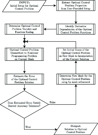
Refer to caption
Figure 3: Flowchart of the โ„‚โ€‹๐”พโ€‹โ„™โ€‹๐•†โ€‹โ„™โ€‹๐•Šโ„‚๐”พโ„™๐•†โ„™๐•Š{\mathbb{CGPOPS}} Algorithm.

5 Examples

โ„‚โ€‹๐”พโ€‹โ„™โ€‹๐•†โ€‹โ„™โ€‹๐•Šโ„‚๐”พโ„™๐•†โ„™๐•Š{\mathbb{CGPOPS}} is now demonstrated on five examples taken from the open literature. The first example is the hyper-sensitive optimal control problem from Ref.ย [47] and demonstrates the ability of โ„‚โ€‹๐”พโ€‹โ„™โ€‹๐•†โ€‹โ„™โ€‹๐•Šโ„‚๐”พโ„™๐•†โ„™๐•Š{\mathbb{CGPOPS}} to efficiently solve problems that have rapid changes in dynamics in particular regions of the solution. The second example is the reusable launch vehicle entry problem taken from Ref.ย [14] and demonstrates the efficiency of โ„‚โ€‹๐”พโ€‹โ„™โ€‹๐•†โ€‹โ„™โ€‹๐•Šโ„‚๐”พโ„™๐•†โ„™๐•Š{\mathbb{CGPOPS}} on a more realistic problem. The third example is the space station attitude optimal control problem taken from Refs.ย [48] and [14] and demonstrates the efficiency of โ„‚โ€‹๐”พโ€‹โ„™โ€‹๐•†โ€‹โ„™โ€‹๐•Šโ„‚๐”พโ„™๐•†โ„™๐•Š{\mathbb{CGPOPS}} on a problem whose solution is highly non-intuitive. The fourth example is a free-flying robot problem taken from Ref.ย [14] and demonstrates the ability of โ„‚โ€‹๐”พโ€‹โ„™โ€‹๐•†โ€‹โ„™โ€‹๐•Šโ„‚๐”พโ„™๐•†โ„™๐•Š{\mathbb{CGPOPS}} to solve a bang-bang optimal control problem using discontinuity detection. The fifth example is a multiple-stage launch vehicle ascent problem taken from Refs.ย [50, 7, 14] and demonstrates the ability of โ„‚โ€‹๐”พโ€‹โ„™โ€‹๐•†โ€‹โ„™โ€‹๐•Šโ„‚๐”พโ„™๐•†โ„™๐•Š{\mathbb{CGPOPS}} to solve a problem with multiple-phases.

All five examples were solved using the open-source NLP solver IPOPT [12] in second derivative (full Newton) mode with the publicly available multifrontal massively parallel sparse direct linear solver MA57 [60]. All results were obtained using the differential form of the LGR collocation method and various forms of the aforementioned hโ€‹pโ„Ž๐‘hp mesh refinement method using default NLP solver settings and the automatic scaling routine in โ„‚โ€‹๐”พโ€‹โ„™โ€‹๐•†โ€‹โ„™โ€‹๐•Šโ„‚๐”พโ„™๐•†โ„™๐•Š{\mathbb{CGPOPS}}. For โ„‚โ€‹๐”พโ€‹โ„™โ€‹๐•†โ€‹โ„™โ€‹๐•Šโ„‚๐”พโ„™๐•†โ„™๐•Š{\mathbb{CGPOPS}}, all first- and second-order derivatives for the NLP solver were obtained using hyper-dual derivative approximations as described in Sectionย 4.4.3 with a perturbation step size of h=1โ„Ž1h=1. All solutions obtained by โ„‚โ€‹๐”พโ€‹โ„™โ€‹๐•†โ€‹โ„™โ€‹๐•Šโ„‚๐”พโ„™๐•†โ„™๐•Š{\mathbb{CGPOPS}} are compared against the solutions obtained using the previously developed MATLAB software ๐”พโ€‹โ„™โ€‹๐•†โ€‹โ„™โ€‹๐•Šโˆ’๐•€โ€‹๐•€๐”พโ„™๐•†โ„™๐•Š๐•€๐•€\mathbb{GPOPS-II} [10] which also employs hโ€‹pโ„Ž๐‘hp LGR collocation methods. For ๐”พโ€‹โ„™โ€‹๐•†โ€‹โ„™โ€‹๐•Šโˆ’๐•€โ€‹๐•€๐”พโ„™๐•†โ„™๐•Š๐•€๐•€\mathbb{GPOPS-II}, the first- and second-order derivatives for the NLP solver were obtained using the automatic differentiation software ADiGator [61] for all examples except the fifth example which used sparse central finite-differences. All computations were performed on a 2.9 GHz Intel Core i7 MacBook Pro running MAC OS-X version 10.13.6 (High Sierra) with 16GB 2133MHz LPDDR3 of RAM. C++ files were compiled using Apple LLVM version 9.1.0 (clang-1000.10.44.2). All m-scripts were executed using MATLAB Version R2016a (build 9.0.0.341360). All plots were created using MATLAB Version R2016a (build 9.0.0.341360).

5.1 Example 1: Hyper-Sensitive Problem

Consider the following hyper-sensitive optimal control problem taken from Ref.ย [47]. The objective is to minimize the cost functional

๐’ฅ=12โ€‹โˆซ0tf(x2+u2)โ€‹๐‘‘t,๐’ฅ12superscriptsubscript0subscript๐‘ก๐‘“superscript๐‘ฅ2superscript๐‘ข2differential-d๐‘ก{\cal{J}}=\frac{1}{2}\int_{0}^{t_{f}}(x^{2}+u^{2})~{}dt~{}, (46)

subject to the dynamic constraints

xห™=โˆ’x3+u,ห™๐‘ฅsuperscript๐‘ฅ3๐‘ข\dot{x}=-x^{3}+u~{}, (47)

and the boundary conditions

xโ€‹(0)=1,xโ€‹(tf)=1.5,๐‘ฅ01missing-subexpression๐‘ฅsubscript๐‘ก๐‘“1.5\begin{array}[]{lcl}x(0)=1~{},&&x(t_{f})=1.5~{},\end{array} (48)

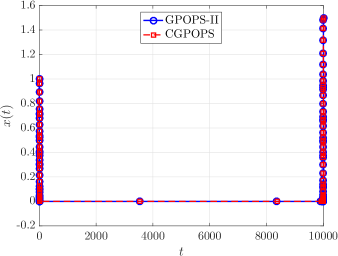
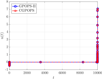
where tf=10000subscript๐‘ก๐‘“10000t_{f}=10000. It is known for a sufficiently large value of tfsubscript๐‘ก๐‘“t_{f} the interesting behavior in the solution for the optimal control problem defined by Eqs.ย (46) โ€“ (48) occurs near t=0๐‘ก0t=0 and t=tf๐‘กsubscript๐‘ก๐‘“t=t_{f} (see Ref.ย [47] for details), while the vast majority of the solution is a constant. Given the structure of the solution, a majority of collocation points need to be placed near t=0๐‘ก0t=0 and t=tf๐‘กsubscript๐‘ก๐‘“t=t_{f}.

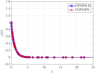
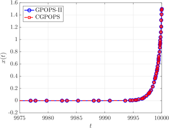
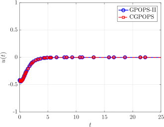
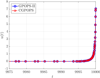
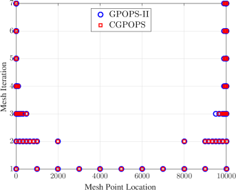
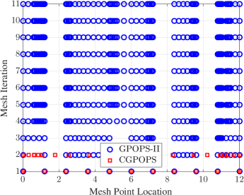
The hyper-sensitive optimal control problem was solved using โ„‚โ€‹๐”พโ€‹โ„™โ€‹๐•†โ€‹โ„™โ€‹๐•Šโ„‚๐”พโ„™๐•†โ„™๐•Š{\mathbb{CGPOPS}} with the mesh refinement methods hโ€‹pโ„Ž๐‘hp-I(3,10), hโ€‹pโ„Ž๐‘hp-II(3,10), hโ€‹pโ„Ž๐‘hp-III(3,10), and hโ€‹pโ„Ž๐‘hp-IV(3,10) on an initial mesh of ten evenly spaced mesh intervals with three LGR points per mesh interval. The NLP solver and mesh refinement accuracy tolerances were set to 10โˆ’7superscript10710^{-7} and 10โˆ’6superscript10610^{-6}, respectively. The solution obtained using โ„‚โ€‹๐”พโ€‹โ„™โ€‹๐•†โ€‹โ„™โ€‹๐•Šโ„‚๐”พโ„™๐•†โ„™๐•Š{\mathbb{CGPOPS}} with the hโ€‹pโ„Ž๐‘hp-IV(3,10) method is shown in Fig.ย 4 alongside the solution obtained using ๐”พโ€‹โ„™โ€‹๐•†โ€‹โ„™โ€‹๐•Šโˆ’๐•€โ€‹๐•€๐”พโ„™๐•†โ„™๐•Š๐•€๐•€\mathbb{GPOPS-II} [10] with the hโ€‹pโ„Ž๐‘hp-IV(3,10) method. It is seen that the โ„‚โ€‹๐”พโ€‹โ„™โ€‹๐•†โ€‹โ„™โ€‹๐•Šโ„‚๐”พโ„™๐•†โ„™๐•Š{\mathbb{CGPOPS}} and ๐”พโ€‹โ„™โ€‹๐•†โ€‹โ„™โ€‹๐•Šโˆ’๐•€โ€‹๐•€๐”พโ„™๐•†โ„™๐•Š๐•€๐•€\mathbb{GPOPS-II} solutions are in excellent agreement. Moreover, the optimal cost obtained using โ„‚โ€‹๐”พโ€‹โ„™โ€‹๐•†โ€‹โ„™โ€‹๐•Šโ„‚๐”พโ„™๐•†โ„™๐•Š{\mathbb{CGPOPS}} and ๐”พโ€‹โ„™โ€‹๐•†โ€‹โ„™โ€‹๐•Šโˆ’๐•€โ€‹๐•€๐”พโ„™๐•†โ„™๐•Š๐•€๐•€\mathbb{GPOPS-II} are extremely close, with values of 3.36205593.36205593.3620559 and 3.36205593.36205593.3620559, respectively, agreeing to the seventh decimal place. Additionally, the computational time required by โ„‚โ€‹๐”พโ€‹โ„™โ€‹๐•†โ€‹โ„™โ€‹๐•Šโ„‚๐”พโ„™๐•†โ„™๐•Š{\mathbb{CGPOPS}} and ๐”พโ€‹โ„™โ€‹๐•†โ€‹โ„™โ€‹๐•Šโˆ’๐•€โ€‹๐•€๐”พโ„™๐•†โ„™๐•Š๐•€๐•€\mathbb{GPOPS-II} to solve the optimal control problem was 0.21530.21530.2153 seconds and 1.52301.52301.5230 seconds, respectively. In order to demonstrate how โ„‚โ€‹๐”พโ€‹โ„™โ€‹๐•†โ€‹โ„™โ€‹๐•Šโ„‚๐”พโ„™๐•†โ„™๐•Š{\mathbb{CGPOPS}} is capable of capturing the interesting features of the optimal solution, Fig.ย 5 shows the solution on the intervals tโˆˆ[0,25]๐‘ก025t\in[0,25] (near the initial time) and tโˆˆ[9975,10000]๐‘ก997510000t\in[9975,10000] (near the final time). It is seen that โ„‚โ€‹๐”พโ€‹โ„™โ€‹๐•†โ€‹โ„™โ€‹๐•Šโ„‚๐”พโ„™๐•†โ„™๐•Š{\mathbb{CGPOPS}} accurately captures the rapid decay from xโ€‹(0)=1๐‘ฅ01x(0)=1 and the rapid growth to meet the terminal condition xโ€‹(tf)=1.5๐‘ฅsubscript๐‘ก๐‘“1.5x(t_{f})=1.5, with the density of the mesh points near t=0๐‘ก0t=0 and t=tf๐‘กsubscript๐‘ก๐‘“t=t_{f} increasing as the mesh refinement progresses. Additionally, Fig.ย 6 shows the mesh refinement history. Finally, Tablesย 1 โ€“ 4 show the estimated error on each mesh, where it is seen that the solution error decreases steadily with each mesh refinement iteration for all hโ€‹pโ„Ž๐‘hp methods employed.

Table 1: Performance of โ„‚โ€‹๐”พโ€‹โ„™โ€‹๐•†โ€‹โ„™โ€‹๐•Šโ„‚๐”พโ„™๐•†โ„™๐•Š{\mathbb{CGPOPS}} on Example 1 using hโ€‹pโ„Ž๐‘hp-I(3,10).
Mesh Estimated Number of Estimated Number of
Iteration Error (โ„‚โ€‹๐”พโ€‹โ„™โ€‹๐•†โ€‹โ„™โ€‹๐•Šโ„‚๐”พโ„™๐•†โ„™๐•Š{\mathbb{CGPOPS}}) Collocation Error (๐”พโ€‹โ„™โ€‹๐•†โ€‹โ„™โ€‹๐•Šโˆ’๐•€โ€‹๐•€๐”พโ„™๐•†โ„™๐•Š๐•€๐•€\mathbb{GPOPS-II}) Collocation
Number hโ€‹pโ„Ž๐‘hp-I(3,10) Points hโ€‹pโ„Ž๐‘hp-I(3,10) Points
111 28.2728.2728.27 313131 28.2728.2728.27 313131
222 4.0904.0904.090 676767 4.0904.0904.090 676767
333 7.060ร—10โˆ’17.060superscript1017.060\times 10^{-1} 101101101 7.060ร—10โˆ’17.060superscript1017.060\times 10^{-1} 101101101
444 1.661ร—10โˆ’11.661superscript1011.661\times 10^{-1} 134134134 1.661ร—10โˆ’11.661superscript1011.661\times 10^{-1} 134134134
555 1.476ร—10โˆ’21.476superscript1021.476\times 10^{-2} 158158158 1.476ร—10โˆ’21.476superscript1021.476\times 10^{-2} 158158158
666 1.139ร—10โˆ’31.139superscript1031.139\times 10^{-3} 191191191 1.139ร—10โˆ’31.139superscript1031.139\times 10^{-3} 191191191
777 7.557ร—10โˆ’77.557superscript1077.557\times 10^{-7} 218218218 7.557ร—10โˆ’77.557superscript1077.557\times 10^{-7} 218218218
Table 2: Performance of โ„‚โ€‹๐”พโ€‹โ„™โ€‹๐•†โ€‹โ„™โ€‹๐•Šโ„‚๐”พโ„™๐•†โ„™๐•Š{\mathbb{CGPOPS}} on Example 1 using hโ€‹pโ„Ž๐‘hp-II(3,10).
Mesh Estimated Number of Estimated Number of
Iteration Error (โ„‚โ€‹๐”พโ€‹โ„™โ€‹๐•†โ€‹โ„™โ€‹๐•Šโ„‚๐”พโ„™๐•†โ„™๐•Š{\mathbb{CGPOPS}}) Collocation Error (๐”พโ€‹โ„™โ€‹๐•†โ€‹โ„™โ€‹๐•Šโˆ’๐•€โ€‹๐•€๐”พโ„™๐•†โ„™๐•Š๐•€๐•€\mathbb{GPOPS-II}) Collocation
Number hโ€‹pโ„Ž๐‘hp-II(3,10) Points hโ€‹pโ„Ž๐‘hp-II(3,10) Points
111 28.2728.2728.27 313131 28.2728.2728.27 313131
222 1.6671.6671.667 656565 1.6671.6671.667 656565
333 3.1933.1933.193 106106106 3.1933.1933.193 106106106
444 1.557ร—10โˆ’11.557superscript1011.557\times 10^{-1} 140140140 1.557ร—10โˆ’11.557superscript1011.557\times 10^{-1} 140140140
555 4.142ร—10โˆ’14.142superscript1014.142\times 10^{-1} 165165165 4.142ร—10โˆ’14.142superscript1014.142\times 10^{-1} 165165165
666 1.261ร—10โˆ’21.261superscript1021.261\times 10^{-2} 185185185 1.261ร—10โˆ’21.261superscript1021.261\times 10^{-2} 185185185
777 4.423ร—10โˆ’24.423superscript1024.423\times 10^{-2} 204204204 4.423ร—10โˆ’24.423superscript1024.423\times 10^{-2} 204204204
888 4.707ร—10โˆ’44.707superscript1044.707\times 10^{-4} 209209209 4.707ร—10โˆ’44.707superscript1044.707\times 10^{-4} 209209209
999 1.090ร—10โˆ’31.090superscript1031.090\times 10^{-3} 226226226 1.090ร—10โˆ’31.090superscript1031.090\times 10^{-3} 226226226
101010 7.742ร—10โˆ’67.742superscript1067.742\times 10^{-6} 247247247 7.742ร—10โˆ’67.742superscript1067.742\times 10^{-6} 247247247
111111 7.470ร—10โˆ’77.470superscript1077.470\times 10^{-7} 250250250 7.470ร—10โˆ’77.470superscript1077.470\times 10^{-7} 250250250
Table 3: Performance of โ„‚โ€‹๐”พโ€‹โ„™โ€‹๐•†โ€‹โ„™โ€‹๐•Šโ„‚๐”พโ„™๐•†โ„™๐•Š{\mathbb{CGPOPS}} on Example 1 using hโ€‹pโ„Ž๐‘hp-III(3,10).
Mesh Estimated Number of Estimated Number of
Iteration Error (โ„‚โ€‹๐”พโ€‹โ„™โ€‹๐•†โ€‹โ„™โ€‹๐•Šโ„‚๐”พโ„™๐•†โ„™๐•Š{\mathbb{CGPOPS}}) Collocation Error (๐”พโ€‹โ„™โ€‹๐•†โ€‹โ„™โ€‹๐•Šโˆ’๐•€โ€‹๐•€๐”พโ„™๐•†โ„™๐•Š๐•€๐•€\mathbb{GPOPS-II}) Collocation
Number hโ€‹pโ„Ž๐‘hp-III(3,10) Points hโ€‹pโ„Ž๐‘hp-III(3,10) Points
111 28.2728.2728.27 313131 28.2728.2728.27 313131
222 5.2075.2075.207 222222 5.2075.2075.207 222222
333 5.848ร—10โˆ’15.848superscript1015.848\times 10^{-1} 112112112 5.848ร—10โˆ’15.848superscript1015.848\times 10^{-1} 112112112
444 9.156ร—10โˆ’29.156superscript1029.156\times 10^{-2} 139139139 9.156ร—10โˆ’29.156superscript1029.156\times 10^{-2} 142142142
555 5.732ร—10โˆ’35.732superscript1035.732\times 10^{-3} 115115115 5.732ร—10โˆ’35.732superscript1035.732\times 10^{-3} 112112112
666 9.927ร—10โˆ’59.927superscript1059.927\times 10^{-5} 146146146 9.927ร—10โˆ’59.927superscript1059.927\times 10^{-5} 146146146
777 2.451ร—10โˆ’52.451superscript1052.451\times 10^{-5} 153153153 2.451ร—10โˆ’52.451superscript1052.451\times 10^{-5} 153153153
888 8.237ร—10โˆ’78.237superscript1078.237\times 10^{-7} 160160160 8.237ร—10โˆ’78.237superscript1078.237\times 10^{-7} 160160160
Table 4: Performance of โ„‚โ€‹๐”พโ€‹โ„™โ€‹๐•†โ€‹โ„™โ€‹๐•Šโ„‚๐”พโ„™๐•†โ„™๐•Š{\mathbb{CGPOPS}} on Example 1 using hโ€‹pโ„Ž๐‘hp-IV(3,10).
Mesh Estimated Number of Estimated Number of
Iteration Error (โ„‚โ€‹๐”พโ€‹โ„™โ€‹๐•†โ€‹โ„™โ€‹๐•Šโ„‚๐”พโ„™๐•†โ„™๐•Š{\mathbb{CGPOPS}}) Collocation Error (๐”พโ€‹โ„™โ€‹๐•†โ€‹โ„™โ€‹๐•Šโˆ’๐•€โ€‹๐•€๐”พโ„™๐•†โ„™๐•Š๐•€๐•€\mathbb{GPOPS-II}) Collocation
Number hโ€‹pโ„Ž๐‘hp-IV(3,10) Points hโ€‹pโ„Ž๐‘hp-IV(3,10) Points
111 28.2728.2728.27 313131 28.2728.2728.27 313131
222 4.7634.7634.763 464646 4.7634.7634.763 464646
333 8.214ร—10โˆ’18.214superscript1018.214\times 10^{-1} 525252 8.214ร—10โˆ’18.214superscript1018.214\times 10^{-1} 555555
444 1.813ร—10โˆ’11.813superscript1011.813\times 10^{-1} 555555 1.813ร—10โˆ’11.813superscript1011.813\times 10^{-1} 585858
555 2.114ร—10โˆ’22.114superscript1022.114\times 10^{-2} 616161 2.114ร—10โˆ’22.114superscript1022.114\times 10^{-2} 616161
666 1.688ร—10โˆ’31.688superscript1031.688\times 10^{-3} 878787 1.688ร—10โˆ’31.688superscript1031.688\times 10^{-3} 878787
777 8.991ร—10โˆ’78.991superscript1078.991\times 10^{-7} 106106106 8.991ร—10โˆ’78.991superscript1078.991\times 10^{-7} 106106106
Refer to caption
(a) xโ€‹(t)๐‘ฅ๐‘กx(t) vs.ย t๐‘กt.
Refer to caption
(b) uโ€‹(t)๐‘ข๐‘กu(t) vs.ย t๐‘กt.
Figure 4: โ„‚โ€‹๐”พโ€‹โ„™โ€‹๐•†โ€‹โ„™โ€‹๐•Šโ„‚๐”พโ„™๐•†โ„™๐•Š{\mathbb{CGPOPS}} and ๐”พโ€‹โ„™โ€‹๐•†โ€‹โ„™โ€‹๐•Šโˆ’๐•€โ€‹๐•€๐”พโ„™๐•†โ„™๐•Š๐•€๐•€\mathbb{GPOPS-II} Solutions to Example 1 using hโ€‹pโ„Ž๐‘hp-IV(3,10).
Refer to caption
(a) xโ€‹(t)๐‘ฅ๐‘กx(t) vs.ย t๐‘กt Near t=0๐‘ก0t=0.
Refer to caption
(b) xโ€‹(t)๐‘ฅ๐‘กx(t) vs.ย t๐‘กt Near t=tf๐‘กsubscript๐‘ก๐‘“t=t_{f}.
Refer to caption
(c) uโ€‹(t)๐‘ข๐‘กu(t) vs.ย t๐‘กt Near t=0๐‘ก0t=0.
Refer to caption
(d) uโ€‹(t)๐‘ข๐‘กu(t) vs.ย t๐‘กt Near t=tf๐‘กsubscript๐‘ก๐‘“t=t_{f}.
Figure 5: โ„‚โ€‹๐”พโ€‹โ„™โ€‹๐•†โ€‹โ„™โ€‹๐•Šโ„‚๐”พโ„™๐•†โ„™๐•Š{\mathbb{CGPOPS}} and ๐”พโ€‹โ„™โ€‹๐•†โ€‹โ„™โ€‹๐•Šโˆ’๐•€โ€‹๐•€๐”พโ„™๐•†โ„™๐•Š๐•€๐•€\mathbb{GPOPS-II} Solutions to Example 1 Near t=0๐‘ก0t=0 and t=tf๐‘กsubscript๐‘ก๐‘“t=t_{f} using hโ€‹pโ„Ž๐‘hp-IV(3,10).
Refer to caption
Figure 6: โ„‚โ€‹๐”พโ€‹โ„™โ€‹๐•†โ€‹โ„™โ€‹๐•Šโ„‚๐”พโ„™๐•†โ„™๐•Š{\mathbb{CGPOPS}} and ๐”พโ€‹โ„™โ€‹๐•†โ€‹โ„™โ€‹๐•Šโˆ’๐•€โ€‹๐•€๐”พโ„™๐•†โ„™๐•Š๐•€๐•€\mathbb{GPOPS-II} Mesh Refinement History for Example 1 Using hโ€‹pโ„Ž๐‘hp-IV(3,10).

5.2 Example 2: Reusable Launch Vehicle Entry

Consider the following optimal control problem of maximizing the crossrange during the atmospheric entry of a reusable launch vehicle taken from Ref.ย [14] where the numerical values in Ref.ย [14] are converted from English units to SI units. Maximize the cost functional

๐’ฅ=ฯ•โ€‹(๐“‰๐’ป),๐’ฅitalic-ฯ•subscript๐“‰๐’ป\cal{J}=\phi(t_{f})~{}, (49)

subject to the dynamic constraints

rห™=vโ€‹sinโกฮณ,ฮธห™=vโ€‹cosโกฮณโ€‹sinโกฯˆrโ€‹cosโกฯ•,ฯ•ห™=vโ€‹cosโกฮณโ€‹cosโกฯˆr,vห™=โˆ’Dmโˆ’gโ€‹sinโกฮณ,ฮณห™=Lโ€‹cosโกฯƒmโ€‹vโˆ’(gvโˆ’vr)โ€‹cosโกฮณ,ฯˆห™=Lโ€‹sinโกฯƒmโ€‹vโ€‹cosโกฮณ+vโ€‹cosโกฮณโ€‹sinโกฯˆโ€‹tanโกฯ•r,ห™๐‘Ÿ๐‘ฃ๐›พmissing-subexpressionห™๐œƒ๐‘ฃ๐›พ๐œ“๐‘Ÿitalic-ฯ•ห™italic-ฯ•๐‘ฃ๐›พ๐œ“๐‘Ÿmissing-subexpressionห™๐‘ฃ๐ท๐‘š๐‘”๐›พห™๐›พ๐ฟ๐œŽ๐‘š๐‘ฃ๐‘”๐‘ฃ๐‘ฃ๐‘Ÿ๐›พmissing-subexpressionห™๐œ“๐ฟ๐œŽ๐‘š๐‘ฃ๐›พ๐‘ฃ๐›พ๐œ“italic-ฯ•๐‘Ÿ\begin{array}[]{lclclcl}\dot{r}&=&v\sin\gamma~{},&&\dot{\theta}&=&\displaystyle\frac{v\cos\gamma\sin\psi}{r\cos\phi}~{},\\ \dot{\phi}&=&\displaystyle\frac{v\cos\gamma\cos\psi}{r}~{},&&\dot{v}&=&\displaystyle-\frac{D}{m}-g\sin\gamma~{},\\ \dot{\gamma}&=&\displaystyle\frac{L\cos\sigma}{mv}-\left(\frac{g}{v}-\frac{v}{r}\right)\cos\gamma~{},&&\dot{\psi}&=&\displaystyle\frac{L\sin\sigma}{mv\cos\gamma}+\frac{v\cos\gamma\sin\psi\tan\phi}{r}~{},\end{array} (50)

and the boundary conditions

hโ€‹(0)=79248โ€‹ย km,hโ€‹(tf)=24384โ€‹ย km,ฮธโ€‹(0)=0โ€‹ย deg,ฮธโ€‹(tf)=Free,ฯ•โ€‹(0)=0โ€‹ย deg,ฯ•โ€‹(tf)=Free,vโ€‹(0)=7.803โ€‹ย km/s,vโ€‹(tf)=0.762โ€‹ย km/s,ฮณโ€‹(0)=โˆ’1โ€‹ย deg,ฮณโ€‹(tf)=โˆ’5โ€‹ย deg,ฯˆโ€‹(0)=90โ€‹ย deg,ฯˆโ€‹(tf)=Free,โ„Ž079248ย kmmissing-subexpressionโ„Žsubscript๐‘ก๐‘“24384ย km๐œƒ00ย degmissing-subexpression๐œƒsubscript๐‘ก๐‘“Freeitalic-ฯ•00ย degmissing-subexpressionitalic-ฯ•subscript๐‘ก๐‘“Free๐‘ฃ07.803ย km/smissing-subexpression๐‘ฃsubscript๐‘ก๐‘“0.762ย km/s๐›พ01ย degmissing-subexpression๐›พsubscript๐‘ก๐‘“5ย deg๐œ“090ย degmissing-subexpression๐œ“subscript๐‘ก๐‘“Free\begin{array}[]{lclclcl}h(0)&=&79248\textrm{ km}~{},&&h(t_{f})&=&24384\textrm{ km}~{},\\ \theta(0)&=&0\textrm{ deg}~{},&&\theta(t_{f})&=&\textrm{Free}~{},\\ \phi(0)&=&0\textrm{ deg}~{},&&\phi(t_{f})&=&\textrm{Free}~{},\\ v(0)&=&7.803\textrm{ km/s}~{},&&v(t_{f})&=&0.762\textrm{ km/s}~{},\\ \gamma(0)&=&-1\textrm{ deg}~{},&&\gamma(t_{f})&=&-5\textrm{ deg}~{},\\ \psi(0)&=&90\textrm{ deg}~{},&&\psi(t_{f})&=&\textrm{Free}~{},\end{array} (51)

where r=h+Re๐‘Ÿโ„Žsubscript๐‘…๐‘’r=h+R_{e} is the geocentric radius, hโ„Žh is the altitude, Resubscript๐‘…๐‘’R_{e} is the polar radius of the Earth, ฮธ๐œƒ\theta is the longitude, ฯ•italic-ฯ•\phi is the latitude, v๐‘ฃv is the speed, ฮณ๐›พ\gamma is the flight path angle, ฯˆ๐œ“\psi is the azimuth angle and m๐‘šm is the mass of the vehicle. Furthermore, the aerodynamic and gravitational forces are computed as

D=ฯโ€‹v2โ€‹Sโ€‹CD/2,L=ฯโ€‹v2โ€‹Sโ€‹CL/2,g=ฮผ/r2,๐ท๐œŒsuperscript๐‘ฃ2๐‘†subscript๐ถ๐ท2missing-subexpression๐ฟ๐œŒsuperscript๐‘ฃ2๐‘†subscript๐ถ๐ฟ2missing-subexpression๐‘”๐œ‡superscript๐‘Ÿ2\begin{array}[]{lclclclclcl}D&=&\rho v^{2}SC_{D}/2~{},&&L&=&\rho v^{2}SC_{L}/2~{},&&g&=&\mu/r^{2}~{},\end{array} (52)

where ฯ=ฯ0โ€‹expโก(โˆ’h/H)๐œŒsubscript๐œŒ0โ„Ž๐ป\rho=\rho_{0}\exp(-h/H) is the atmospheric density, ฯ0subscript๐œŒ0\rho_{0} is the density at sea level, H๐ปH is the density scale height, S๐‘†S is the vehicle reference area, CDsubscript๐ถ๐ทC_{D} is the coefficient of drag, CLsubscript๐ถ๐ฟC_{L} is the coefficient of lift, and ฮผ๐œ‡\mu is the gravitational parameter.

The reusable launch vehicle entry optimal control problem defined by Eqs.ย (49) โ€“ (52) was solved using โ„‚โ€‹๐”พโ€‹โ„™โ€‹๐•†โ€‹โ„™โ€‹๐•Šโ„‚๐”พโ„™๐•†โ„™๐•Š{\mathbb{CGPOPS}} with the hโ€‹pโ„Ž๐‘hp-I(4,10), hโ€‹pโ„Ž๐‘hp-II(4,10), hโ€‹pโ„Ž๐‘hp-III(4,10), and hโ€‹pโ„Ž๐‘hp-IV(4,10) methods on an initial mesh consisting of ten evenly spaced mesh intervals with four LGR points per mesh interval. The NLP solver and mesh refinement accuracy tolerances were both set to 10โˆ’7superscript10710^{-7}. The initial guess of the state was a straight line over the duration tโˆˆ[0,1000]๐‘ก01000t\in[0,1000] between the known initial and final components of the state or a constant at the initial values of the components of the state whose terminal values are not specified, while the initial guess of both controls was zero. Tablesย 5 โ€“ 8 show the performance of both โ„‚โ€‹๐”พโ€‹โ„™โ€‹๐•†โ€‹โ„™โ€‹๐•Šโ„‚๐”พโ„™๐•†โ„™๐•Š{\mathbb{CGPOPS}} and ๐”พโ€‹โ„™โ€‹๐•†โ€‹โ„™โ€‹๐•Šโˆ’๐•€โ€‹๐•€๐”พโ„™๐•†โ„™๐•Š๐•€๐•€\mathbb{GPOPS-II} on this example for the four hโ€‹pโ„Ž๐‘hp methods, where the mesh refinement history is nearly identical for each of the respective methods. The solution obtained using โ„‚โ€‹๐”พโ€‹โ„™โ€‹๐•†โ€‹โ„™โ€‹๐•Šโ„‚๐”พโ„™๐•†โ„™๐•Š{\mathbb{CGPOPS}} with the hโ€‹pโ„Ž๐‘hp-III(4,10) method is shown in Figs.ย 7a โ€“ 8b alongside the solution obtained using the software ๐”พโ€‹โ„™โ€‹๐•†โ€‹โ„™โ€‹๐•Šโˆ’๐•€โ€‹๐•€๐”พโ„™๐•†โ„™๐•Š๐•€๐•€\mathbb{GPOPS-II} [10] with the hโ€‹pโ„Ž๐‘hp-III(4,10) method, where it is seen that the two solutions obtained are essentially identical. It is noted that the optimal cost obtained by โ„‚โ€‹๐”พโ€‹โ„™โ€‹๐•†โ€‹โ„™โ€‹๐•Šโ„‚๐”พโ„™๐•†โ„™๐•Š{\mathbb{CGPOPS}} and ๐”พโ€‹โ„™โ€‹๐•†โ€‹โ„™โ€‹๐•Šโˆ’๐•€โ€‹๐•€๐”พโ„™๐•†โ„™๐•Š๐•€๐•€\mathbb{GPOPS-II} are also identical at 0.596276390.596276390.59627639 and 0.596276390.596276390.59627639, respectively. Finally, the computational time used by โ„‚โ€‹๐”พโ€‹โ„™โ€‹๐•†โ€‹โ„™โ€‹๐•Šโ„‚๐”พโ„™๐•†โ„™๐•Š{\mathbb{CGPOPS}} is approximately half the amount of time required by ๐”พโ€‹โ„™โ€‹๐•†โ€‹โ„™โ€‹๐•Šโˆ’๐•€โ€‹๐•€๐”พโ„™๐•†โ„™๐•Š๐•€๐•€\mathbb{GPOPS-II} to solve the optimal control problem, taking 0.9105ย seconds and 1.9323 seconds, respectively.

Table 5: Performance of โ„‚โ€‹๐”พโ€‹โ„™โ€‹๐•†โ€‹โ„™โ€‹๐•Šโ„‚๐”พโ„™๐•†โ„™๐•Š{\mathbb{CGPOPS}} on Example 2 using hโ€‹pโ„Ž๐‘hp-I(4,10).
Mesh Estimated Number of Estimated Number of
Iteration Error (โ„‚โ€‹๐”พโ€‹โ„™โ€‹๐•†โ€‹โ„™โ€‹๐•Šโ„‚๐”พโ„™๐•†โ„™๐•Š{\mathbb{CGPOPS}}) Collocation Error (๐”พโ€‹โ„™โ€‹๐•†โ€‹โ„™โ€‹๐•Šโˆ’๐•€โ€‹๐•€๐”พโ„™๐•†โ„™๐•Š๐•€๐•€\mathbb{GPOPS-II}) Collocation
Number hโ€‹pโ„Ž๐‘hp-I(4,10) Points hโ€‹pโ„Ž๐‘hp-I(4,10) Points
111 2.463ร—10โˆ’32.463superscript1032.463\times 10^{-3} 414141 2.463ร—10โˆ’32.463superscript1032.463\times 10^{-3} 414141
222 9.891ร—10โˆ’59.891superscript1059.891\times 10^{-5} 103103103 9.896ร—10โˆ’59.896superscript1059.896\times 10^{-5} 103103103
333 3.559ร—10โˆ’63.559superscript1063.559\times 10^{-6} 118118118 3.559ร—10โˆ’63.559superscript1063.559\times 10^{-6} 118118118
444 3.287ร—10โˆ’73.287superscript1073.287\times 10^{-7} 133133133 3.287ร—10โˆ’73.287superscript1073.287\times 10^{-7} 133133133
555 8.706ร—10โˆ’88.706superscript1088.706\times 10^{-8} 134134134 8.706ร—10โˆ’88.706superscript1088.706\times 10^{-8} 134134134
Table 6: Performance of โ„‚โ€‹๐”พโ€‹โ„™โ€‹๐•†โ€‹โ„™โ€‹๐•Šโ„‚๐”พโ„™๐•†โ„™๐•Š{\mathbb{CGPOPS}} on Example 2 using hโ€‹pโ„Ž๐‘hp-II(4,10).
Mesh Estimated Number of Estimated Number of
Iteration Error (โ„‚โ€‹๐”พโ€‹โ„™โ€‹๐•†โ€‹โ„™โ€‹๐•Šโ„‚๐”พโ„™๐•†โ„™๐•Š{\mathbb{CGPOPS}}) Collocation Error (๐”พโ€‹โ„™โ€‹๐•†โ€‹โ„™โ€‹๐•Šโˆ’๐•€โ€‹๐•€๐”พโ„™๐•†โ„™๐•Š๐•€๐•€\mathbb{GPOPS-II}) Collocation
Number hโ€‹pโ„Ž๐‘hp-II(4,10) Points hโ€‹pโ„Ž๐‘hp-II(4,10) Points
111 2.463ร—10โˆ’32.463superscript1032.463\times 10^{-3} 414141 2.463ร—10โˆ’32.463superscript1032.463\times 10^{-3} 414141
222 6.026ร—10โˆ’66.026superscript1066.026\times 10^{-6} 193193193 6.023ร—10โˆ’66.023superscript1066.023\times 10^{-6} 193193193
333 8.227ร—10โˆ’88.227superscript1088.227\times 10^{-8} 261261261 8.227ร—10โˆ’88.227superscript1088.227\times 10^{-8} 261261261
Table 7: Performance of โ„‚โ€‹๐”พโ€‹โ„™โ€‹๐•†โ€‹โ„™โ€‹๐•Šโ„‚๐”พโ„™๐•†โ„™๐•Š{\mathbb{CGPOPS}} on Example 2 using hโ€‹pโ„Ž๐‘hp-III(4,10).
Mesh Estimated Number of Estimated Number of
Iteration Error (โ„‚โ€‹๐”พโ€‹โ„™โ€‹๐•†โ€‹โ„™โ€‹๐•Šโ„‚๐”พโ„™๐•†โ„™๐•Š{\mathbb{CGPOPS}}) Collocation Error (๐”พโ€‹โ„™โ€‹๐•†โ€‹โ„™โ€‹๐•Šโˆ’๐•€โ€‹๐•€๐”พโ„™๐•†โ„™๐•Š๐•€๐•€\mathbb{GPOPS-II}) Collocation
Number hโ€‹pโ„Ž๐‘hp-III(4,10) Points hโ€‹pโ„Ž๐‘hp-III(4,10) Points
111 2.463ร—10โˆ’32.463superscript1032.463\times 10^{-3} 414141 2.463ร—10โˆ’32.463superscript1032.463\times 10^{-3} 414141
222 2.850ร—10โˆ’52.850superscript1052.850\times 10^{-5} 717171 2.850ร—10โˆ’52.850superscript1052.850\times 10^{-5} 717171
333 2.065ร—10โˆ’62.065superscript1062.065\times 10^{-6} 141141141 2.065ร—10โˆ’62.065superscript1062.065\times 10^{-6} 141141141
444 8.887ร—10โˆ’88.887superscript1088.887\times 10^{-8} 148148148 8.887ร—10โˆ’88.887superscript1088.887\times 10^{-8} 148148148
Table 8: Performance of โ„‚โ€‹๐”พโ€‹โ„™โ€‹๐•†โ€‹โ„™โ€‹๐•Šโ„‚๐”พโ„™๐•†โ„™๐•Š{\mathbb{CGPOPS}} on Example 2 using hโ€‹pโ„Ž๐‘hp-IV(4,10).
Mesh Estimated Number of Estimated Number of
Iteration Error (โ„‚โ€‹๐”พโ€‹โ„™โ€‹๐•†โ€‹โ„™โ€‹๐•Šโ„‚๐”พโ„™๐•†โ„™๐•Š{\mathbb{CGPOPS}}) Collocation Error (๐”พโ€‹โ„™โ€‹๐•†โ€‹โ„™โ€‹๐•Šโˆ’๐•€โ€‹๐•€๐”พโ„™๐•†โ„™๐•Š๐•€๐•€\mathbb{GPOPS-II}) Collocation
Number hโ€‹pโ„Ž๐‘hp-IV(4,10) Points hโ€‹pโ„Ž๐‘hp-IV(4,10) Points
111 2.463ร—10โˆ’32.463superscript1032.463\times 10^{-3} 414141 2.463ร—10โˆ’32.463superscript1032.463\times 10^{-3} 414141
222 2.364ร—10โˆ’52.364superscript1052.364\times 10^{-5} 122122122 3.364ร—10โˆ’53.364superscript1053.364\times 10^{-5} 122122122
333 3.286ร—10โˆ’73.286superscript1073.286\times 10^{-7} 200200200 3.286ร—10โˆ’73.286superscript1073.286\times 10^{-7} 192192192
444 9.561ร—10โˆ’89.561superscript1089.561\times 10^{-8} 203203203 1.285ร—10โˆ’71.285superscript1071.285\times 10^{-7} 194194194
555 โ€“ โ€“ 9.561ร—10โˆ’89.561superscript1089.561\times 10^{-8} 195195195
Refer to caption
(a) hโ€‹(t)โ„Ž๐‘กh(t) vs.ย t๐‘กt.
Refer to caption
(b) vโ€‹(t)๐‘ฃ๐‘กv(t) vs.ย t๐‘กt.
Refer to caption
(c) ฯ•โ€‹(t)italic-ฯ•๐‘ก\phi(t) vs.ย t๐‘กt.
Refer to caption
(d) ฮณโ€‹(t)๐›พ๐‘ก\gamma(t) vs.ย t๐‘กt.
Figure 7: โ„‚โ€‹๐”พโ€‹โ„™โ€‹๐•†โ€‹โ„™โ€‹๐•Šโ„‚๐”พโ„™๐•†โ„™๐•Š{\mathbb{CGPOPS}} and ๐”พโ€‹โ„™โ€‹๐•†โ€‹โ„™โ€‹๐•Šโˆ’๐•€โ€‹๐•€๐”พโ„™๐•†โ„™๐•Š๐•€๐•€\mathbb{GPOPS-II} State Solutions to Example 2 Using hโ€‹pโ„Ž๐‘hp-III(4,10).
Refer to caption
(a) ฮฑโ€‹(t)๐›ผ๐‘ก\alpha(t) vs.ย t๐‘กt.
Refer to caption
(b) ฯƒโ€‹(t)๐œŽ๐‘ก\sigma(t) vs.ย t๐‘กt.
Figure 8: โ„‚โ€‹๐”พโ€‹โ„™โ€‹๐•†โ€‹โ„™โ€‹๐•Šโ„‚๐”พโ„™๐•†โ„™๐•Š{\mathbb{CGPOPS}} and ๐”พโ€‹โ„™โ€‹๐•†โ€‹โ„™โ€‹๐•Šโˆ’๐•€โ€‹๐•€๐”พโ„™๐•†โ„™๐•Š๐•€๐•€\mathbb{GPOPS-II} Control Solutions to Example 2 Using hโ€‹pโ„Ž๐‘hp-III(4,10).
Refer to caption
Figure 9: โ„‚โ€‹๐”พโ€‹โ„™โ€‹๐•†โ€‹โ„™โ€‹๐•Šโ„‚๐”พโ„™๐•†โ„™๐•Š{\mathbb{CGPOPS}} and ๐”พโ€‹โ„™โ€‹๐•†โ€‹โ„™โ€‹๐•Šโˆ’๐•€โ€‹๐•€๐”พโ„™๐•†โ„™๐•Š๐•€๐•€\mathbb{GPOPS-II} Mesh Refinement History for Example 2 Using hโ€‹pโ„Ž๐‘hp-III(4,10).

5.3 Example 3: Space Station Attitude Control

Consider the following space station attitude control optimal control problem taken from Refs.ย [48] and [14]. Minimize the cost functional

๐’ฅ=12โ€‹โˆซ๐“‰0๐“‰๐’ป๐ฎ๐–ณโ€‹๐ฎโ€‹๐’น๐“‰,๐’ฅ12superscriptsubscriptsubscript๐“‰0subscript๐“‰๐’ปsuperscript๐ฎ๐–ณ๐ฎdifferential-d๐“‰\cal{J}=\displaystyle\frac{1}{2}\int_{t_{0}}^{t_{f}}{\bf{u}}^{\sf T}{\bf{u}}~{}dt~{}, (53)

subject to the dynamic constraints

๐Ž=๐‰โˆ’1โ€‹{๐‰gโ€‹gโ€‹(๐ซ)โˆ’๐ŽโŠ—โ€‹[๐‰โ€‹๐Ž+๐ก]โˆ’๐ฎ},๐ซห™=12โ€‹[๐ซ๐ซ๐–ณ+๐ˆ+๐ซ]โ€‹[๐Žโˆ’๐Žโ€‹(๐ซ)],๐กห™=๐ฎ,๐Žsuperscript๐‰1subscript๐‰๐‘”๐‘”๐ซsuperscript๐Žtensor-productdelimited-[]๐‰๐Ž๐ก๐ฎห™๐ซ12delimited-[]superscript๐ซ๐ซ๐–ณ๐ˆ๐ซdelimited-[]๐Ž๐Ž๐ซห™๐ก๐ฎ\begin{array}[]{lcl}\boldsymbol{\omega}&=&\displaystyle{\bf{J}}^{-1}\left\{\boldsymbol{\tau}_{gg}({\bf{r}})-\boldsymbol{\omega}^{\otimes}\left[{\bf{J}}\boldsymbol{\omega}+{\bf{h}}\right]-{\bf{u}}\right\}~{},\\ \dot{{\bf{r}}}&=&\displaystyle\frac{1}{2}\left[{\bf{r}}{\bf{r}}^{\sf T}+{\bf{I}}+{\bf{r}}\right]\left[\boldsymbol{\omega}-\boldsymbol{\omega}({\bf{r}})\right]~{},\\ \dot{{\bf{h}}}&=&{\bf{u}}~{},\end{array} (54)

the inequality path constraint

โ€–๐กโ€–โ‰คhmax,norm๐กsubscriptโ„Ž\left\|{\bf{h}}\right\|\leq h_{\max}~{}, (55)

and the boundary conditions

t0=0,tf=1800,๐Žโ€‹(0)=๐Žยฏ0,๐ซโ€‹(0)=๐ซยฏ0,๐กโ€‹(0)=๐กยฏ0,๐ŸŽ=๐‰โˆ’1โ€‹{๐‰gโ€‹gโ€‹(๐ซโ€‹(tf))โˆ’๐ŽโŠ—โ€‹(tf)โ€‹[๐‰โ€‹๐Žโ€‹(tf)+๐กโ€‹(tf)]},๐ŸŽ=12โ€‹[๐ซโ€‹(tf)โ€‹๐ซTโ€‹(tf)+๐ˆ+๐ซโ€‹(tf)]โ€‹[๐Žโ€‹(tf)โˆ’๐Ž0โ€‹(๐ซโ€‹(tf))],subscript๐‘ก00missing-subexpressionsubscript๐‘ก๐‘“1800๐Ž0subscriptยฏ๐Ž0missing-subexpression๐ซ0subscriptยฏ๐ซ0missing-subexpression๐ก0subscriptยฏ๐ก00superscript๐‰1subscript๐‰๐‘”๐‘”๐ซsubscript๐‘ก๐‘“superscript๐Žtensor-productsubscript๐‘ก๐‘“delimited-[]๐‰๐Žsubscript๐‘ก๐‘“๐กsubscript๐‘ก๐‘“012delimited-[]๐ซsubscript๐‘ก๐‘“superscript๐ซTsubscript๐‘ก๐‘“๐ˆ๐ซsubscript๐‘ก๐‘“delimited-[]๐Žsubscript๐‘ก๐‘“subscript๐Ž0๐ซsubscript๐‘ก๐‘“\begin{array}[]{l}\begin{array}[]{rclclcl}\hskip 11.56346ptt_{0}&=&0~{},&&\hskip 14.45377ptt_{f}&=&1800~{},\vspace{3pt}\\ \end{array}\vspace{3pt}\\ \begin{array}[]{rclclclclcl}\boldsymbol{\omega}(0)&=&\bar{\boldsymbol{\omega}}_{0}~{},&&{\bf{r}}(0)&=&\bar{{\bf{r}}}_{0}~{},&&{\bf{h}}(0)&=&\bar{{\bf{h}}}_{0}~{},\vspace{3pt}\\ \end{array}\\ \begin{array}[]{rcl}\hskip 13.73148pt\mathbf{0}&=&\displaystyle\mathbf{J}^{-1}\left\{\boldsymbol{\tau}_{gg}(\mathbf{r}(t_{f}))-\boldsymbol{\omega}^{\otimes}(t_{f})\left[\mathbf{J}\boldsymbol{\omega}(t_{f})+\mathbf{h}(t_{f})\right]\right\}~{},\vspace{3pt}\\ \mathbf{0}&=&\displaystyle\frac{1}{2}\left[\mathbf{r}(t_{f})\mathbf{r}^{\textsf{T}}(t_{f})+\mathbf{I}+\mathbf{r}(t_{f})\right]\left[\boldsymbol{\omega}(t_{f})-\boldsymbol{\omega}_{0}(\mathbf{r}(t_{f}))\right]~{},\end{array}\end{array} (56)

where (๐Ž,๐ซ,๐ก)๐Ž๐ซ๐ก(\boldsymbol{\omega},{\bf{r}},{\bf{h}}) is the state and ๐ฎ๐ฎ{\bf{u}} is the control. In this formulation ๐Ž๐Ž\boldsymbol{\omega} is the angular velocity, ๐ซ๐ซ{\bf{r}} is the Euler-Rodrigues parameter vector, ๐ก๐ก{\bf{h}} is the angular momentum, and ๐ฎ๐ฎ{\bf{u}} is the input moment (and is the control). Furthermore,

๐Ž0โ€‹(๐ซ)=โˆ’ฯ‰orbโ€‹๐‚2,๐‰gโ€‹g=3โ€‹ฯ‰orb2โ€‹๐‚3โŠ—โ€‹๐‰๐‚3,ฯ‰orb=0.6511โ€‹ฯ€180,hmax=10000,subscript๐Ž0๐ซsubscript๐œ”orbsubscript๐‚2missing-subexpressionsubscript๐‰๐‘”๐‘”3superscriptsubscript๐œ”orb2superscriptsubscript๐‚3tensor-productsubscript๐‰๐‚3subscript๐œ”orb0.6511๐œ‹180missing-subexpressionsubscriptโ„Ž10000\begin{array}[]{lclclcl}\boldsymbol{\omega}_{0}({\bf{r}})&=&-\omega_{\textrm{orb}}{\bf{C}}_{2}~{},&&\boldsymbol{\tau}_{gg}&=&3\omega_{\textrm{orb}}^{2}{\bf{C}}_{3}^{\otimes}{\bf{J}}{\bf{C}}_{3}~{},\vspace{3pt}\\ \omega_{\textrm{orb}}&=&\displaystyle 0.6511\frac{\pi}{180}~{},&&h_{\max}&=&10000~{},\vspace{3pt}\\ \end{array} (57)

and ๐‚2subscript๐‚2{\bf{C}}_{2} and ๐‚3subscript๐‚3{\bf{C}}_{3} are the second and third column, respectively, of the matrix

๐‚=๐ˆ+21+๐ซ๐–ณโ€‹๐ซโ€‹(๐ซโŠ—โ€‹๐ซโŠ—โˆ’๐ซโŠ—).๐‚๐ˆ21superscript๐ซ๐–ณ๐ซsuperscript๐ซtensor-productsuperscript๐ซtensor-productsuperscript๐ซtensor-product{\bf{C}}={\bf{I}}+\frac{2}{1+{\bf{r}}^{\sf T}{\bf{r}}}\left({\bf{r}}^{\otimes}{\bf{r}}^{\otimes}-{\bf{r}}^{\otimes}\right)~{}. (58)

In this example the matrix ๐‰๐‰{\bf{J}} is given as

๐‰=[2.80701911616ร—1074.822509936ร—105โˆ’1.71675094448ร—1074.822509936ร—1059.5144639344ร—1076.02604448ร—104โˆ’1.71675094448ร—1076.02604448ร—1047.6594401336ร—107],๐‰delimited-[]2.80701911616superscript1074.822509936superscript1051.71675094448superscript1074.822509936superscript1059.5144639344superscript1076.02604448superscript1041.71675094448superscript1076.02604448superscript1047.6594401336superscript107{\bf{J}}=\left[\begin{array}[]{ccc}2.80701911616\times 10^{7}&4.822509936\times 10^{5}&-1.71675094448\times 10^{7}\\ 4.822509936\times 10^{5}&9.5144639344\times 10^{7}&6.02604448\times 10^{4}\\ -1.71675094448\times 10^{7}&6.02604448\times 10^{4}&7.6594401336\times 10^{7}\end{array}\right]~{}, (59)

while the initial conditions ๐Žยฏ0subscriptยฏ๐Ž0\bar{\boldsymbol{\omega}}_{0}, ๐ซยฏ0subscriptยฏ๐ซ0\bar{{\bf{r}}}_{0}, and ๐กยฏ0subscriptยฏ๐ก0\bar{{\bf{h}}}_{0} are

๐Žยฏ0=[โˆ’9.5380685844896ร—10โˆ’6โˆ’1.1363312657036ร—10โˆ’3+5.3472801108427ร—10โˆ’6],๐ซยฏ0=[2.9963689649816ร—10โˆ’31.5334477761054ร—10โˆ’13.8359805613992ร—10โˆ’3],๐กยฏ0=[500050005000].subscriptยฏ๐Ž0delimited-[]9.5380685844896superscript1061.1363312657036superscript1035.3472801108427superscript106missing-subexpressionsubscriptยฏ๐ซ0delimited-[]2.9963689649816superscript1031.5334477761054superscript1013.8359805613992superscript103missing-subexpressionsubscriptยฏ๐ก0delimited-[]500050005000\begin{array}[]{l}\begin{array}[]{lcl}\bar{\boldsymbol{\omega}}_{0}&=&\left[\begin{array}[]{c}-9.5380685844896\times 10^{-6}\\ -1.1363312657036\times 10^{-3}\\ +5.3472801108427\times 10^{-6}\end{array}\right]~{},\end{array}\\ \\ \begin{array}[]{lclclcl}~{}\bar{{\bf{r}}}_{0}&=&\left[\begin{array}[]{c}2.9963689649816\times 10^{-3}\\ 1.5334477761054\times 10^{-1}\\ 3.8359805613992\times 10^{-3}\end{array}\right]~{},&&\bar{{\bf{h}}}_{0}&=&\left[\begin{array}[]{c}5000\\ 5000\\ 5000\end{array}\right]~{}.\end{array}\end{array} (60)

A more detailed description of this problem, including all of the constants ๐‰๐‰{\bf{J}}, ๐Žยฏ0subscriptยฏ๐Ž0\bar{\boldsymbol{\omega}}_{0}, ๐ซยฏ0subscriptยฏ๐ซ0\bar{{\bf{r}}}_{0}, and ๐กยฏ0subscriptยฏ๐ก0\bar{{\bf{h}}}_{0}, can be found in [48] or [14].

The optimal control problem defined by Eqs.ย (53) โ€“ (60) was solved using โ„‚โ€‹๐”พโ€‹โ„™โ€‹๐•†โ€‹โ„™โ€‹๐•Šโ„‚๐”พโ„™๐•†โ„™๐•Š{\mathbb{CGPOPS}} with the hโ€‹pโ„Ž๐‘hp-I(4,10), hโ€‹pโ„Ž๐‘hp-II(4,10), hโ€‹pโ„Ž๐‘hp-III(4,10), and hโ€‹pโ„Ž๐‘hp-IV(4,10) methods on an initial mesh consisting of ten uniformly spaced mesh intervals and four LGR points per mesh interval. The NLP solver and mesh refinement accuracy tolerances were set to 10โˆ’7superscript10710^{-7} and 10โˆ’6superscript10610^{-6}, respectively. The initial guess was a constant over the time interval tโˆˆ[0,1800]๐‘ก01800t\in[0,1800], where the constant was (๐Žยฏ0,๐ซยฏ0,๐กยฏ0)subscriptยฏ๐Ž0subscriptยฏ๐ซ0subscriptยฏ๐ก0(\bar{\boldsymbol{\omega}}_{0},\bar{{\bf{r}}}_{0},\bar{{\bf{h}}}_{0}) for the state and zero for the control. The state and control solutions obtained using โ„‚โ€‹๐”พโ€‹โ„™โ€‹๐•†โ€‹โ„™โ€‹๐•Šโ„‚๐”พโ„™๐•†โ„™๐•Š{\mathbb{CGPOPS}} are shown, respectively, in Fig.ย 10 and 11 alongside the solution obtained using the optimal control software ๐”พโ€‹โ„™โ€‹๐•†โ€‹โ„™โ€‹๐•Šโˆ’๐•€โ€‹๐•€๐”พโ„™๐•†โ„™๐•Š๐•€๐•€\mathbb{GPOPS-II} [10] with the hโ€‹pโ„Ž๐‘hp-I(4,10). It is seen that the โ„‚โ€‹๐”พโ€‹โ„™โ€‹๐•†โ€‹โ„™โ€‹๐•Šโ„‚๐”พโ„™๐•†โ„™๐•Š{\mathbb{CGPOPS}} solution matches extremely well with the ๐”พโ€‹โ„™โ€‹๐•†โ€‹โ„™โ€‹๐•Šโˆ’๐•€โ€‹๐•€๐”พโ„™๐•†โ„™๐•Š๐•€๐•€\mathbb{GPOPS-II} solution. Moreover, the optimal cost obtained using โ„‚โ€‹๐”พโ€‹โ„™โ€‹๐•†โ€‹โ„™โ€‹๐•Šโ„‚๐”พโ„™๐•†โ„™๐•Š{\mathbb{CGPOPS}} and ๐”พโ€‹โ„™โ€‹๐•†โ€‹โ„™โ€‹๐•Šโˆ’๐•€โ€‹๐•€๐”พโ„™๐•†โ„™๐•Š๐•€๐•€\mathbb{GPOPS-II} are essentially the same, with values of 3.5867511ร—10โˆ’63.5867511superscript1063.5867511\times 10^{-6} and 3.5867511ร—10โˆ’63.5867511superscript1063.5867511\times 10^{-6}, respectively. Finally, the computational time required by โ„‚โ€‹๐”พโ€‹โ„™โ€‹๐•†โ€‹โ„™โ€‹๐•Šโ„‚๐”พโ„™๐•†โ„™๐•Š{\mathbb{CGPOPS}} and ๐”พโ€‹โ„™โ€‹๐•†โ€‹โ„™โ€‹๐•Šโˆ’๐•€โ€‹๐•€๐”พโ„™๐•†โ„™๐•Š๐•€๐•€\mathbb{GPOPS-II} to solve the optimal control problem was 0.53380.53380.5338 seconds and 2.76962.76962.7696 seconds, respectively.

Table 9: Performance of โ„‚โ€‹๐”พโ€‹โ„™โ€‹๐•†โ€‹โ„™โ€‹๐•Šโ„‚๐”พโ„™๐•†โ„™๐•Š{\mathbb{CGPOPS}} on Example 3 using hโ€‹pโ„Ž๐‘hp-I(4,10).
Mesh Estimated Number of Estimated Number of
Iteration Error (โ„‚โ€‹๐”พโ€‹โ„™โ€‹๐•†โ€‹โ„™โ€‹๐•Šโ„‚๐”พโ„™๐•†โ„™๐•Š{\mathbb{CGPOPS}}) Collocation Error (๐”พโ€‹โ„™โ€‹๐•†โ€‹โ„™โ€‹๐•Šโˆ’๐•€โ€‹๐•€๐”พโ„™๐•†โ„™๐•Š๐•€๐•€\mathbb{GPOPS-II}) Collocation
Number hโ€‹pโ„Ž๐‘hp-I(4,10) Points hโ€‹pโ„Ž๐‘hp-I(4,10) Points
111 9.409ร—10โˆ’69.409superscript1069.409\times 10^{-6} 414141 9.409ร—10โˆ’69.409superscript1069.409\times 10^{-6} 414141
222 6.496ร—10โˆ’76.496superscript1076.496\times 10^{-7} 474747 6.496ร—10โˆ’76.496superscript1076.496\times 10^{-7} 474747
Table 10: Performance of โ„‚โ€‹๐”พโ€‹โ„™โ€‹๐•†โ€‹โ„™โ€‹๐•Šโ„‚๐”พโ„™๐•†โ„™๐•Š{\mathbb{CGPOPS}} on Example 3 using hโ€‹pโ„Ž๐‘hp-II(4,10).
Mesh Estimated Number of Estimated Number of
Iteration Error (โ„‚โ€‹๐”พโ€‹โ„™โ€‹๐•†โ€‹โ„™โ€‹๐•Šโ„‚๐”พโ„™๐•†โ„™๐•Š{\mathbb{CGPOPS}}) Collocation Error (๐”พโ€‹โ„™โ€‹๐•†โ€‹โ„™โ€‹๐•Šโˆ’๐•€โ€‹๐•€๐”พโ„™๐•†โ„™๐•Š๐•€๐•€\mathbb{GPOPS-II}) Collocation
Number hโ€‹pโ„Ž๐‘hp-II(4,10) Points hโ€‹pโ„Ž๐‘hp-II(4,10) Points
111 9.409ร—10โˆ’69.409superscript1069.409\times 10^{-6} 414141 9.409ร—10โˆ’69.409superscript1069.409\times 10^{-6} 414141
222 2.389ร—10โˆ’62.389superscript1062.389\times 10^{-6} 505050 2.387ร—10โˆ’62.387superscript1062.387\times 10^{-6} 505050
333 7.125ร—10โˆ’77.125superscript1077.125\times 10^{-7} 555555 7.130ร—10โˆ’77.130superscript1077.130\times 10^{-7} 555555
Table 11: Performance of โ„‚โ€‹๐”พโ€‹โ„™โ€‹๐•†โ€‹โ„™โ€‹๐•Šโ„‚๐”พโ„™๐•†โ„™๐•Š{\mathbb{CGPOPS}} on Example 3 using hโ€‹pโ„Ž๐‘hp-III(4,10).
Mesh Estimated Number of Estimated Number of
Iteration Error (โ„‚โ€‹๐”พโ€‹โ„™โ€‹๐•†โ€‹โ„™โ€‹๐•Šโ„‚๐”พโ„™๐•†โ„™๐•Š{\mathbb{CGPOPS}}) Collocation Error (๐”พโ€‹โ„™โ€‹๐•†โ€‹โ„™โ€‹๐•Šโˆ’๐•€โ€‹๐•€๐”พโ„™๐•†โ„™๐•Š๐•€๐•€\mathbb{GPOPS-II}) Collocation
Number hโ€‹pโ„Ž๐‘hp-III(4,10) Points hโ€‹pโ„Ž๐‘hp-III(4,10) Points
111 9.409ร—10โˆ’69.409superscript1069.409\times 10^{-6} 414141 9.409ร—10โˆ’69.409superscript1069.409\times 10^{-6} 414141
222 9.542ร—10โˆ’79.542superscript1079.542\times 10^{-7} 505050 9.559ร—10โˆ’79.559superscript1079.559\times 10^{-7} 505050
Table 12: Performance of โ„‚โ€‹๐”พโ€‹โ„™โ€‹๐•†โ€‹โ„™โ€‹๐•Šโ„‚๐”พโ„™๐•†โ„™๐•Š{\mathbb{CGPOPS}} on Example 3 using hโ€‹pโ„Ž๐‘hp-IV(4,10).
Mesh Estimated Number of Estimated Number of
Iteration Error (โ„‚โ€‹๐”พโ€‹โ„™โ€‹๐•†โ€‹โ„™โ€‹๐•Šโ„‚๐”พโ„™๐•†โ„™๐•Š{\mathbb{CGPOPS}}) Collocation Error (๐”พโ€‹โ„™โ€‹๐•†โ€‹โ„™โ€‹๐•Šโˆ’๐•€โ€‹๐•€๐”พโ„™๐•†โ„™๐•Š๐•€๐•€\mathbb{GPOPS-II}) Collocation
Number hโ€‹pโ„Ž๐‘hp-IV(4,10) Points hโ€‹pโ„Ž๐‘hp-IV(4,10) Points
111 9.409ร—10โˆ’69.409superscript1069.409\times 10^{-6} 414141 9.409ร—10โˆ’69.409superscript1069.409\times 10^{-6} 414141
222 1.049ร—10โˆ’71.049superscript1071.049\times 10^{-7} 535353 1.046ร—10โˆ’71.046superscript1071.046\times 10^{-7} 535353
333 7.125ร—10โˆ’77.125superscript1077.125\times 10^{-7} 575757 7.130ร—10โˆ’77.130superscript1077.130\times 10^{-7} 575757
Refer to caption
(a) ฯ‰1โ€‹(t)subscript๐œ”1๐‘ก\omega_{1}(t) vs.ย t๐‘กt.
Refer to caption
(b) ฯ‰2โ€‹(t)subscript๐œ”2๐‘ก\omega_{2}(t) vs.ย t๐‘กt.
Refer to caption
(c) ฯ‰3โ€‹(t)subscript๐œ”3๐‘ก\omega_{3}(t) vs.ย t๐‘กt.
Refer to caption
(d) r1โ€‹(t)subscript๐‘Ÿ1๐‘กr_{1}(t) vs.ย t๐‘กt.
Refer to caption
(e) r2โ€‹(t)subscript๐‘Ÿ2๐‘กr_{2}(t) vs.ย t๐‘กt.
Refer to caption
(f) r3โ€‹(t)subscript๐‘Ÿ3๐‘กr_{3}(t) vs.ย t๐‘กt.
Figure 10: โ„‚โ€‹๐”พโ€‹โ„™โ€‹๐•†โ€‹โ„™โ€‹๐•Šโ„‚๐”พโ„™๐•†โ„™๐•Š{\mathbb{CGPOPS}} and ๐”พโ€‹โ„™โ€‹๐•†โ€‹โ„™โ€‹๐•Šโˆ’๐•€โ€‹๐•€๐”พโ„™๐•†โ„™๐•Š๐•€๐•€\mathbb{GPOPS-II} Solutions to Example 3 Using with the NLP Solver IPOPT and a Mesh Refinement Tolerance of 10โˆ’6superscript10610^{-6} using hโ€‹pโ„Ž๐‘hp-I(4,10).
Refer to caption
(a) h1โ€‹(t)subscriptโ„Ž1๐‘กh_{1}(t) vs.ย t๐‘กt.
Refer to caption
(b) h2โ€‹(t)subscriptโ„Ž2๐‘กh_{2}(t) vs.ย t๐‘กt.
Refer to caption
(c) h3โ€‹(t)subscriptโ„Ž3๐‘กh_{3}(t) vs.ย t๐‘กt.
Refer to caption
(d) u1โ€‹(t)subscript๐‘ข1๐‘กu_{1}(t) vs.ย t๐‘กt.
Refer to caption
(e) u2โ€‹(t)subscript๐‘ข2๐‘กu_{2}(t) vs.ย t๐‘กt.
Refer to caption
(f) u3โ€‹(t)subscript๐‘ข3๐‘กu_{3}(t) vs.ย t๐‘กt.
Figure 11: โ„‚โ€‹๐”พโ€‹โ„™โ€‹๐•†โ€‹โ„™โ€‹๐•Šโ„‚๐”พโ„™๐•†โ„™๐•Š{\mathbb{CGPOPS}} and ๐”พโ€‹โ„™โ€‹๐•†โ€‹โ„™โ€‹๐•Šโˆ’๐•€โ€‹๐•€๐”พโ„™๐•†โ„™๐•Š๐•€๐•€\mathbb{GPOPS-II} Solutions to Example 3 Using with the NLP Solver IPOPT and a Mesh Refinement Tolerance of 10โˆ’6superscript10610^{-6} using hโ€‹pโ„Ž๐‘hp-I(4,10).

5.4 Example 4: Free-Flying Robot Problem

Consider the following free-flying robot optimal control problem taken from Refs.ย [14] and [49]. The objective is to minimize the cost functional

๐’ฅ=โˆซ0๐“‰๐’ป(๐“Š1+๐“Š2+๐“Š3+๐“Š4)โ€‹๐’น๐“‰,๐’ฅsuperscriptsubscript0subscript๐“‰๐’ปsubscript๐“Š1subscript๐“Š2subscript๐“Š3subscript๐“Š4differential-d๐“‰\cal{J}=\int_{0}^{t_{f}}(u_{1}+u_{2}+u_{3}+u_{4})dt~{}, (61)

subject to the dynamic constraints

xห™=vx,yห™=vy,vxห™=(F1+F2)โ€‹cosโก(ฮธ),vyห™=(F1+F2)โ€‹sinโก(ฮธ),ฮธห™=ฯ‰,ฯ‰ห™=ฮฑโ€‹F1โˆ’ฮฒโ€‹F2,ห™๐‘ฅsubscript๐‘ฃ๐‘ฅmissing-subexpressionห™๐‘ฆsubscript๐‘ฃ๐‘ฆห™subscript๐‘ฃ๐‘ฅsubscript๐น1subscript๐น2๐œƒmissing-subexpressionห™subscript๐‘ฃ๐‘ฆsubscript๐น1subscript๐น2๐œƒห™๐œƒ๐œ”missing-subexpressionห™๐œ”๐›ผsubscript๐น1๐›ฝsubscript๐น2\begin{array}[]{lclclcl}\dot{x}&=&v_{x}~{},&&\dot{y}&=&v_{y}~{},\\ \dot{v_{x}}&=&(F_{1}+F_{2})\cos(\theta)~{},&&\dot{v_{y}}&=&(F_{1}+F_{2})\sin(\theta)~{},\\ \dot{\theta}&=&\omega~{},&&\dot{\omega}&=&\alpha F_{1}-\beta F_{2}~{},\\ \end{array} (62)

the control inequality constraints

0โ‰คuiโ‰ค1,(i=1,2,3,4),Fiโ‰ค1,(i=1,2),formulae-sequence0subscript๐‘ข๐‘–1๐‘–1234missing-subexpressionsubscript๐น๐‘–1๐‘–12\begin{array}[]{lcl}0\leq u_{i}\leq 1~{},\quad(i=1,2,3,4)~{},&&\quad F_{i}\leq 1~{},~{}\quad(i=1,2)~{},\end{array} (63)

and the boundary conditions

xโ€‹(0)=โˆ’10,xโ€‹(tf)=0,yโ€‹(0)=โˆ’10,yโ€‹(tf)=0,vxโ€‹(0)=0,vxโ€‹(tf)=0,vyโ€‹(0)=0,vyโ€‹(tf)=0,ฮธโ€‹(0)=ฯ€2,ฮธโ€‹(tf)=0,ฯ‰โ€‹(0)=0,ฯ‰โ€‹(tf)=0,๐‘ฅ010missing-subexpression๐‘ฅsubscript๐‘ก๐‘“0missing-subexpression๐‘ฆ010missing-subexpression๐‘ฆsubscript๐‘ก๐‘“0subscript๐‘ฃ๐‘ฅ00missing-subexpressionsubscript๐‘ฃ๐‘ฅsubscript๐‘ก๐‘“0missing-subexpressionsubscript๐‘ฃ๐‘ฆ00missing-subexpressionsubscript๐‘ฃ๐‘ฆsubscript๐‘ก๐‘“0๐œƒ0๐œ‹2missing-subexpression๐œƒsubscript๐‘ก๐‘“0missing-subexpression๐œ”00missing-subexpression๐œ”subscript๐‘ก๐‘“0\begin{array}[]{lclclcl}x(0)=-10~{},&&x(t_{f})=0~{},&&y(0)=-10~{},&&y(t_{f})=0~{},\\ v_{x}(0)=0~{},&&v_{x}(t_{f})=0~{},&&v_{y}(0)=0~{},&&v_{y}(t_{f})=0~{},\\ \theta(0)=\frac{\pi}{2}~{},&&\theta(t_{f})=0~{},&&\omega(0)=0~{},&&\omega(t_{f})=0~{},\end{array} (64)

where

F1=u1โˆ’u2,F2=u3โˆ’u4,ฮฑ=0.2,ฮฒ=0.2.subscript๐น1subscript๐‘ข1subscript๐‘ข2missing-subexpressionsubscript๐น2subscript๐‘ข3subscript๐‘ข4missing-subexpression๐›ผ0.2missing-subexpression๐›ฝ0.2\begin{array}[]{lclclcl}F_{1}=u_{1}-u_{2}~{},&&F_{2}=u_{3}-u_{4}~{},&&\alpha=0.2~{},&&\beta=0.2~{}.\end{array} (65)

It is known that the optimal control problem defined by Eqs.ย (61) โ€“ (65) is a bang-bang optimal control problem, as the Hamiltonian is linear with respect to the control. Given the structure of the solution, the hโ€‹pโ„Ž๐‘hp-BB(3,10) mesh refinement method [59] is also employed to solve this example.

The free-flying robot optimal control problem was solved using โ„‚โ€‹๐”พโ€‹โ„™โ€‹๐•†โ€‹โ„™โ€‹๐•Šโ„‚๐”พโ„™๐•†โ„™๐•Š{\mathbb{CGPOPS}} with the mesh refinement methods hโ€‹pโ„Ž๐‘hp-I(3,10), hโ€‹pโ„Ž๐‘hp-II(3,10), hโ€‹pโ„Ž๐‘hp-III(3,10), hโ€‹pโ„Ž๐‘hp-IV(3,10), and hโ€‹pโ„Ž๐‘hp-BB(3,10) on an initial mesh of ten evenly spaced mesh intervals with five LGR points per mesh interval. The NLP solver and mesh refinement accuracy tolerances were set to 10โˆ’9superscript10910^{-9} and 10โˆ’7superscript10710^{-7}, respectively. The solution obtained using โ„‚โ€‹๐”พโ€‹โ„™โ€‹๐•†โ€‹โ„™โ€‹๐•Šโ„‚๐”พโ„™๐•†โ„™๐•Š{\mathbb{CGPOPS}} with the hโ€‹pโ„Ž๐‘hp-BB(3,10) method is shown in Figs.ย 13 and 14 alongside the solution obtained with ๐”พโ€‹โ„™โ€‹๐•†โ€‹โ„™โ€‹๐•Šโˆ’๐•€โ€‹๐•€๐”พโ„™๐•†โ„™๐•Š๐•€๐•€\mathbb{GPOPS-II} [10] with the hโ€‹pโ„Ž๐‘hp-II(3,10) method. It is seen that the โ„‚โ€‹๐”พโ€‹โ„™โ€‹๐•†โ€‹โ„™โ€‹๐•Šโ„‚๐”พโ„™๐•†โ„™๐•Š{\mathbb{CGPOPS}} and ๐”พโ€‹โ„™โ€‹๐•†โ€‹โ„™โ€‹๐•Šโˆ’๐•€โ€‹๐•€๐”พโ„™๐•†โ„™๐•Š๐•€๐•€\mathbb{GPOPS-II} solutions are in excellent agreement. Moreover, the optimal cost obtained using โ„‚โ€‹๐”พโ€‹โ„™โ€‹๐•†โ€‹โ„™โ€‹๐•Šโ„‚๐”พโ„™๐•†โ„™๐•Š{\mathbb{CGPOPS}} and ๐”พโ€‹โ„™โ€‹๐•†โ€‹โ„™โ€‹๐•Šโˆ’๐•€โ€‹๐•€๐”พโ„™๐•†โ„™๐•Š๐•€๐•€\mathbb{GPOPS-II} are extremely close, with values of 7.91014717.91014717.9101471 and 7.91014217.91014217.9101421, respectively, agreeing to the fifth decimal place. Additionally, the computational time required by โ„‚โ€‹๐”พโ€‹โ„™โ€‹๐•†โ€‹โ„™โ€‹๐•Šโ„‚๐”พโ„™๐•†โ„™๐•Š{\mathbb{CGPOPS}} and ๐”พโ€‹โ„™โ€‹๐•†โ€‹โ„™โ€‹๐•Šโˆ’๐•€โ€‹๐•€๐”พโ„™๐•†โ„™๐•Š๐•€๐•€\mathbb{GPOPS-II} to solve the optimal control problem was 0.63130.63130.6313 seconds and 9.18269.18269.1826 seconds, respectively. In order to demonstrate how โ„‚โ€‹๐”พโ€‹โ„™โ€‹๐•†โ€‹โ„™โ€‹๐•Šโ„‚๐”พโ„™๐•†โ„™๐•Š{\mathbb{CGPOPS}} is capable of more effectively capturing the bang-bang control profile of the optimal solution, Fig.ย 14 shows the control solutions obtained using โ„‚โ€‹๐”พโ€‹โ„™โ€‹๐•†โ€‹โ„™โ€‹๐•Šโ„‚๐”พโ„™๐•†โ„™๐•Š{\mathbb{CGPOPS}} and ๐”พโ€‹โ„™โ€‹๐•†โ€‹โ„™โ€‹๐•Šโˆ’๐•€โ€‹๐•€๐”พโ„™๐•†โ„™๐•Š๐•€๐•€\mathbb{GPOPS-II} with their most effective mesh refinement methods for this example, hโ€‹pโ„Ž๐‘hp-BB(3,10) and hโ€‹pโ„Ž๐‘hp-II(3,10), respectively. It is seen that โ„‚โ€‹๐”พโ€‹โ„™โ€‹๐•†โ€‹โ„™โ€‹๐•Šโ„‚๐”พโ„™๐•†โ„™๐•Š{\mathbb{CGPOPS}} exactly captures the switching points for all eight discontinuities, while the solution obtained using ๐”พโ€‹โ„™โ€‹๐•†โ€‹โ„™โ€‹๐•Šโˆ’๐•€โ€‹๐•€๐”พโ„™๐•†โ„™๐•Š๐•€๐•€\mathbb{GPOPS-II} has fluctuations in the control near the discontinuities for the third and fourth components, as may be observed from Figs.ย 14c,14d, and 14f. Additionally, Fig.ย 12 shows the mesh refinement history for โ„‚โ€‹๐”พโ€‹โ„™โ€‹๐•†โ€‹โ„™โ€‹๐•Šโ„‚๐”พโ„™๐•†โ„™๐•Š{\mathbb{CGPOPS}} with the hโ€‹pโ„Ž๐‘hp-BB(3,10) method and ๐”พโ€‹โ„™โ€‹๐•†โ€‹โ„™โ€‹๐•Šโˆ’๐•€โ€‹๐•€๐”พโ„™๐•†โ„™๐•Š๐•€๐•€\mathbb{GPOPS-II} with the hโ€‹pโ„Ž๐‘hp-II(3,10) method where โ„‚โ€‹๐”พโ€‹โ„™โ€‹๐•†โ€‹โ„™โ€‹๐•Šโ„‚๐”พโ„™๐•†โ„™๐•Š{\mathbb{CGPOPS}} only requires a single mesh refinement iteration to solve, while ๐”พโ€‹โ„™โ€‹๐•†โ€‹โ„™โ€‹๐•Šโˆ’๐•€โ€‹๐•€๐”พโ„™๐•†โ„™๐•Š๐•€๐•€\mathbb{GPOPS-II} takes nine mesh refinement iterations to solve. Finally, Tablesย 13 โ€“ 17 show the estimated error on each mesh, where it is seen that the solution error decreases steadily with each mesh refinement iteration for all hโ€‹pโ„Ž๐‘hp methods employed.

Table 13: Performance of โ„‚โ€‹๐”พโ€‹โ„™โ€‹๐•†โ€‹โ„™โ€‹๐•Šโ„‚๐”พโ„™๐•†โ„™๐•Š{\mathbb{CGPOPS}} on Example 4 using hโ€‹pโ„Ž๐‘hp-I(3,10).
Mesh Estimated Number of Estimated Number of
Iteration Error (โ„‚โ€‹๐”พโ€‹โ„™โ€‹๐•†โ€‹โ„™โ€‹๐•Šโ„‚๐”พโ„™๐•†โ„™๐•Š{\mathbb{CGPOPS}}) Collocation Error (๐”พโ€‹โ„™โ€‹๐•†โ€‹โ„™โ€‹๐•Šโˆ’๐•€โ€‹๐•€๐”พโ„™๐•†โ„™๐•Š๐•€๐•€\mathbb{GPOPS-II}) Collocation
Number hโ€‹pโ„Ž๐‘hp-I(3,10) Points hโ€‹pโ„Ž๐‘hp-I(3,10) Points
111 5.7636ร—10โˆ’45.7636superscript1045.7636\times 10^{-4} 505050 5.7636ร—10โˆ’45.7636superscript1045.7636\times 10^{-4} 505050
222 2.3428ร—10โˆ’42.3428superscript1042.3428\times 10^{-4} 828282 1.2977ร—10โˆ’41.2977superscript1041.2977\times 10^{-4} 828282
333 7.5065ร—10โˆ’57.5065superscript1057.5065\times 10^{-5} 122122122 2.3256ร—10โˆ’42.3256superscript1042.3256\times 10^{-4} 120120120
444 6.2091ร—10โˆ’56.2091superscript1056.2091\times 10^{-5} 157157157 1.1175ร—10โˆ’51.1175superscript1051.1175\times 10^{-5} 161161161
555 9.4236ร—10โˆ’69.4236superscript1069.4236\times 10^{-6} 184184184 6.2093ร—10โˆ’56.2093superscript1056.2093\times 10^{-5} 188188188
666 3.9835ร—10โˆ’63.9835superscript1063.9835\times 10^{-6} 209209209 4.8405ร—10โˆ’64.8405superscript1064.8405\times 10^{-6} 212212212
777 2.8105ร—10โˆ’62.8105superscript1062.8105\times 10^{-6} 224224224 2.8104ร—10โˆ’62.8104superscript1062.8104\times 10^{-6} 234234234
888 8.3276ร—10โˆ’78.3276superscript1078.3276\times 10^{-7} 237237237 1.5139ร—10โˆ’61.5139superscript1061.5139\times 10^{-6} 253253253
999 5.4493ร—10โˆ’75.4493superscript1075.4493\times 10^{-7} 250250250 6.9960ร—10โˆ’76.9960superscript1076.9960\times 10^{-7} 261261261
101010 3.4339ร—10โˆ’73.4339superscript1073.4339\times 10^{-7} 258258258 7.5178ร—10โˆ’77.5178superscript1077.5178\times 10^{-7} 268268268
111111 3.4145ร—10โˆ’73.4145superscript1073.4145\times 10^{-7} 268268268 2.7108ร—10โˆ’72.7108superscript1072.7108\times 10^{-7} 281281281
121212 1.3458ร—10โˆ’71.3458superscript1071.3458\times 10^{-7} 274274274 5.5799ร—10โˆ’75.5799superscript1075.5799\times 10^{-7} 287287287
131313 2.3812ร—10โˆ’72.3812superscript1072.3812\times 10^{-7} 275275275 2.3815ร—10โˆ’72.3815superscript1072.3815\times 10^{-7} 295295295
141414 9.0332ร—10โˆ’89.0332superscript1089.0332\times 10^{-8} 278278278 9.0299ร—10โˆ’89.0299superscript1089.0299\times 10^{-8} 297297297
Table 14: Performance of โ„‚โ€‹๐”พโ€‹โ„™โ€‹๐•†โ€‹โ„™โ€‹๐•Šโ„‚๐”พโ„™๐•†โ„™๐•Š{\mathbb{CGPOPS}} on the Example 4 using hโ€‹pโ„Ž๐‘hp-II(3,10).
Mesh Estimated Number of Estimated Number of
Iteration Error (โ„‚โ€‹๐”พโ€‹โ„™โ€‹๐•†โ€‹โ„™โ€‹๐•Šโ„‚๐”พโ„™๐•†โ„™๐•Š{\mathbb{CGPOPS}}) Collocation Error (๐”พโ€‹โ„™โ€‹๐•†โ€‹โ„™โ€‹๐•Šโˆ’๐•€โ€‹๐•€๐”พโ„™๐•†โ„™๐•Š๐•€๐•€\mathbb{GPOPS-II}) Collocation
Number hโ€‹pโ„Ž๐‘hp-II(3,10) Points hโ€‹pโ„Ž๐‘hp-II(3,10) Points
111 5.7636ร—10โˆ’45.7636superscript1045.7636\times 10^{-4} 505050 5.7636ร—10โˆ’45.7636superscript1045.7636\times 10^{-4} 505050
222 2.3718ร—10โˆ’42.3718superscript1042.3718\times 10^{-4} 989898 1.1649ร—10โˆ’41.1649superscript1041.1649\times 10^{-4} 989898
333 6.4909ร—10โˆ’56.4909superscript1056.4909\times 10^{-5} 162162162 9.3164ร—10โˆ’59.3164superscript1059.3164\times 10^{-5} 146146146
444 2.1470ร—10โˆ’52.1470superscript1052.1470\times 10^{-5} 219219219 1.1244ร—10โˆ’41.1244superscript1041.1244\times 10^{-4} 207207207
555 9.3539ร—10โˆ’69.3539superscript1069.3539\times 10^{-6} 263263263 3.2283ร—10โˆ’63.2283superscript1063.2283\times 10^{-6} 267267267
666 1.0198ร—10โˆ’61.0198superscript1061.0198\times 10^{-6} 297297297 3.5320ร—10โˆ’73.5320superscript1073.5320\times 10^{-7} 302302302
777 1.7028ร—10โˆ’71.7028superscript1071.7028\times 10^{-7} 310310310 2.3505ร—10โˆ’72.3505superscript1072.3505\times 10^{-7} 320320320
888 9.8413ร—10โˆ’89.8413superscript1089.8413\times 10^{-8} 315315315 1.3862ร—10โˆ’71.3862superscript1071.3862\times 10^{-7} 322322322
999 โ€“ โ€“ 1.0431ร—10โˆ’71.0431superscript1071.0431\times 10^{-7} 325325325
101010 โ€“ โ€“ 9.5122ร—10โˆ’89.5122superscript1089.5122\times 10^{-8} 328328328
Table 15: Performance of โ„‚โ€‹๐”พโ€‹โ„™โ€‹๐•†โ€‹โ„™โ€‹๐•Šโ„‚๐”พโ„™๐•†โ„™๐•Š{\mathbb{CGPOPS}} on Example 4 using hโ€‹pโ„Ž๐‘hp-III(3,10).
Mesh Estimated Number of Estimated Number of
Iteration Error (โ„‚โ€‹๐”พโ€‹โ„™โ€‹๐•†โ€‹โ„™โ€‹๐•Šโ„‚๐”พโ„™๐•†โ„™๐•Š{\mathbb{CGPOPS}}) Collocation Error (๐”พโ€‹โ„™โ€‹๐•†โ€‹โ„™โ€‹๐•Šโˆ’๐•€โ€‹๐•€๐”พโ„™๐•†โ„™๐•Š๐•€๐•€\mathbb{GPOPS-II}) Collocation
Number hโ€‹pโ„Ž๐‘hp-III(3,10) Points hโ€‹pโ„Ž๐‘hp-III(3,10) Points
111 5.7636ร—10โˆ’45.7636superscript1045.7636\times 10^{-4} 505050 5.7636ร—10โˆ’45.7636superscript1045.7636\times 10^{-4} 505050
222 1.8489ร—10โˆ’41.8489superscript1041.8489\times 10^{-4} 686868 1.8489ร—10โˆ’41.8489superscript1041.8489\times 10^{-4} 686868
333 5.8497ร—10โˆ’55.8497superscript1055.8497\times 10^{-5} 185185185 5.8497ร—10โˆ’55.8497superscript1055.8497\times 10^{-5} 185185185
444 4.3708ร—10โˆ’64.3708superscript1064.3708\times 10^{-6} 275275275 4.3709ร—10โˆ’64.3709superscript1064.3709\times 10^{-6} 264264264
555 8.2894ร—10โˆ’78.2894superscript1078.2894\times 10^{-7} 349349349 2.3747ร—10โˆ’62.3747superscript1062.3747\times 10^{-6} 324324324
666 4.5337ร—10โˆ’74.5337superscript1074.5337\times 10^{-7} 395395395 2.4780ร—10โˆ’72.4780superscript1072.4780\times 10^{-7} 389389389
777 8.1069ร—10โˆ’88.1069superscript1088.1069\times 10^{-8} 460460460 1.5231ร—10โˆ’71.5231superscript1071.5231\times 10^{-7} 410410410
888 โ€“ โ€“ 1.0142ร—10โˆ’71.0142superscript1071.0142\times 10^{-7} 436436436
999 โ€“ โ€“ 2.1817ร—10โˆ’72.1817superscript1072.1817\times 10^{-7} 437437437
101010 โ€“ โ€“ 8.0985ร—10โˆ’88.0985superscript1088.0985\times 10^{-8} 458458458
Table 16: Performance of โ„‚โ€‹๐”พโ€‹โ„™โ€‹๐•†โ€‹โ„™โ€‹๐•Šโ„‚๐”พโ„™๐•†โ„™๐•Š{\mathbb{CGPOPS}} on Example 4 using hโ€‹pโ„Ž๐‘hp-IV(3,10).
Mesh Estimated Number of Estimated Number of
Iteration Error (โ„‚โ€‹๐”พโ€‹โ„™โ€‹๐•†โ€‹โ„™โ€‹๐•Šโ„‚๐”พโ„™๐•†โ„™๐•Š{\mathbb{CGPOPS}}) Collocation Error (๐”พโ€‹โ„™โ€‹๐•†โ€‹โ„™โ€‹๐•Šโˆ’๐•€โ€‹๐•€๐”พโ„™๐•†โ„™๐•Š๐•€๐•€\mathbb{GPOPS-II}) Collocation
Number hโ€‹pโ„Ž๐‘hp-IV(3,10) Points hโ€‹pโ„Ž๐‘hp-IV(3,10) Points
111 5.7636ร—10โˆ’45.7636superscript1045.7636\times 10^{-4} 505050 5.7636ร—10โˆ’45.7636superscript1045.7636\times 10^{-4} 505050
222 7.2614ร—10โˆ’57.2614superscript1057.2614\times 10^{-5} 100100100 7.2614ร—10โˆ’57.2614superscript1057.2614\times 10^{-5} 100100100
333 5.8350ร—10โˆ’55.8350superscript1055.8350\times 10^{-5} 163163163 5.8350ร—10โˆ’55.8350superscript1055.8350\times 10^{-5} 163163163
444 7.0276ร—10โˆ’67.0276superscript1067.0276\times 10^{-6} 212212212 3.9712ร—10โˆ’63.9712superscript1063.9712\times 10^{-6} 203203203
555 2.9097ร—10โˆ’62.9097superscript1062.9097\times 10^{-6} 259259259 1.9372ร—10โˆ’61.9372superscript1061.9372\times 10^{-6} 249249249
666 5.0338ร—10โˆ’75.0338superscript1075.0338\times 10^{-7} 317317317 7.0224ร—10โˆ’67.0224superscript1067.0224\times 10^{-6} 301301301
777 2.1987ร—10โˆ’72.1987superscript1072.1987\times 10^{-7} 362362362 1.1880ร—10โˆ’61.1880superscript1061.1880\times 10^{-6} 328328328
888 9.8979ร—10โˆ’89.8979superscript1089.8979\times 10^{-8} 376376376 7.4092ร—10โˆ’77.4092superscript1077.4092\times 10^{-7} 347347347
999 โ€“ โ€“ 1.9947ร—10โˆ’71.9947superscript1071.9947\times 10^{-7} 360360360
101010 โ€“ โ€“ 9.1526ร—10โˆ’89.1526superscript1089.1526\times 10^{-8} 373373373
Table 17: Performance of โ„‚โ€‹๐”พโ€‹โ„™โ€‹๐•†โ€‹โ„™โ€‹๐•Šโ„‚๐”พโ„™๐•†โ„™๐•Š{\mathbb{CGPOPS}} on Example 4 using hโ€‹pโ„Ž๐‘hp-BB(3,10).
Mesh Estimated Number of Estimated Number of
Iteration Error (โ„‚โ€‹๐”พโ€‹โ„™โ€‹๐•†โ€‹โ„™โ€‹๐•Šโ„‚๐”พโ„™๐•†โ„™๐•Š{\mathbb{CGPOPS}}) Collocation Error (๐”พโ€‹โ„™โ€‹๐•†โ€‹โ„™โ€‹๐•Šโˆ’๐•€โ€‹๐•€๐”พโ„™๐•†โ„™๐•Š๐•€๐•€\mathbb{GPOPS-II}) Collocation
Number hโ€‹pโ„Ž๐‘hp-BB(3,10) Points hโ€‹pโ„Ž๐‘hp-II(3,10) Points
111 5.7636ร—10โˆ’45.7636superscript1045.7636\times 10^{-4} 505050 5.7636ร—10โˆ’45.7636superscript1045.7636\times 10^{-4} 505050
222 6.2675ร—10โˆ’96.2675superscript1096.2675\times 10^{-9} 108108108 1.1649ร—10โˆ’41.1649superscript1041.1649\times 10^{-4} 989898
333 โ€“ โ€“ 9.3164ร—10โˆ’59.3164superscript1059.3164\times 10^{-5} 146146146
444 โ€“ โ€“ 1.1244ร—10โˆ’41.1244superscript1041.1244\times 10^{-4} 207207207
555 โ€“ โ€“ 3.2283ร—10โˆ’63.2283superscript1063.2283\times 10^{-6} 267267267
666 โ€“ โ€“ 3.5320ร—10โˆ’73.5320superscript1073.5320\times 10^{-7} 302302302
777 โ€“ โ€“ 2.3505ร—10โˆ’72.3505superscript1072.3505\times 10^{-7} 320320320
888 โ€“ โ€“ 1.3862ร—10โˆ’71.3862superscript1071.3862\times 10^{-7} 322322322
999 โ€“ โ€“ 1.0431ร—10โˆ’71.0431superscript1071.0431\times 10^{-7} 325325325
101010 โ€“ โ€“ 9.5122ร—10โˆ’89.5122superscript1089.5122\times 10^{-8} 328328328
Refer to caption
Figure 12: โ„‚โ€‹๐”พโ€‹โ„™โ€‹๐•†โ€‹โ„™โ€‹๐•Šโ„‚๐”พโ„™๐•†โ„™๐•Š{\mathbb{CGPOPS}} and ๐”พโ€‹โ„™โ€‹๐•†โ€‹โ„™โ€‹๐•Šโˆ’๐•€โ€‹๐•€๐”พโ„™๐•†โ„™๐•Š๐•€๐•€\mathbb{GPOPS-II} Mesh Refinement History for Example 4 Using hโ€‹pโ„Ž๐‘hp-BB(3,10) and hโ€‹pโ„Ž๐‘hp-II(3,10), respectively.
Refer to caption
(a) xโ€‹(t)๐‘ฅ๐‘กx(t) vs.ย t๐‘กt.
Refer to caption
(b) yโ€‹(t)๐‘ฆ๐‘กy(t) vs.ย t๐‘กt.
Refer to caption
(c) vxโ€‹(t)subscript๐‘ฃ๐‘ฅ๐‘กv_{x}(t) vs.ย t๐‘กt.
Refer to caption
(d) vyโ€‹(t)subscript๐‘ฃ๐‘ฆ๐‘กv_{y}(t) vs.ย t๐‘กt.
Refer to caption
(e) ฮธโ€‹(t)๐œƒ๐‘ก\theta(t) vs.ย t๐‘กt.
Refer to caption
(f) ฯ‰โ€‹(t)๐œ”๐‘ก\omega(t) vs.ย t๐‘กt.
Figure 13: โ„‚โ€‹๐”พโ€‹โ„™โ€‹๐•†โ€‹โ„™โ€‹๐•Šโ„‚๐”พโ„™๐•†โ„™๐•Š{\mathbb{CGPOPS}} and ๐”พโ€‹โ„™โ€‹๐•†โ€‹โ„™โ€‹๐•Šโˆ’๐•€โ€‹๐•€๐”พโ„™๐•†โ„™๐•Š๐•€๐•€\mathbb{GPOPS-II} State Solutions to Example 4 using hโ€‹pโ„Ž๐‘hp-BB(3,10) and hโ€‹pโ„Ž๐‘hp-II(3,10), respectively.
Refer to caption
(a) u1โ€‹(t)subscript๐‘ข1๐‘กu_{1}(t) vs.ย t๐‘กt.
Refer to caption
(b) u2โ€‹(t)subscript๐‘ข2๐‘กu_{2}(t) vs.ย t๐‘กt.
Refer to caption
(c) u3โ€‹(t)subscript๐‘ข3๐‘กu_{3}(t) vs.ย t๐‘กt.
Refer to caption
(d) u4โ€‹(t)subscript๐‘ข4๐‘กu_{4}(t) vs.ย t๐‘กt.
Refer to caption
(e) F1โ€‹(t)subscript๐น1๐‘กF_{1}(t) vs.ย t๐‘กt.
Refer to caption
(f) F2โ€‹(t)subscript๐น2๐‘กF_{2}(t) vs.ย t๐‘กt.
Figure 14: โ„‚โ€‹๐”พโ€‹โ„™โ€‹๐•†โ€‹โ„™โ€‹๐•Šโ„‚๐”พโ„™๐•†โ„™๐•Š{\mathbb{CGPOPS}} and ๐”พโ€‹โ„™โ€‹๐•†โ€‹โ„™โ€‹๐•Šโˆ’๐•€โ€‹๐•€๐”พโ„™๐•†โ„™๐•Š๐•€๐•€\mathbb{GPOPS-II} Control Solutions to Example 4 using hโ€‹pโ„Ž๐‘hp-BB(3,10) and hโ€‹pโ„Ž๐‘hp-II(3,10), respectively.

5.5 Example 5: Multiple-Stage Launch Vehicle Ascent Problem

The problem considered in this section is the ascent of a multiple-stage launch vehicle. The objective is to maneuver the launch vehicle from the ground to the target orbit while maximizing the remaining fuel in the upper stage. It is noted that this example is found verbatim in Refs.ย [50], [7], and [14]. The problem is modeled using four phases where the objective is to maximize the mass at the end of the fourth phase, that is maximize

๐’ฅ=๐“‚โ€‹(๐“‰๐’ป(4)),๐’ฅ๐“‚superscriptsubscript๐“‰๐’ป4\cal{J}=m(t_{f}^{(4)})~{}, (66)

subject to the dynamic constraints

rห™(p)=๐ฏ(p),vห™(p)=โˆ’ฮผโ€–r(p)โ€–3โ€‹๐ซ(p)+T(p)m(p)โ€‹๐ฎ(p)+๐ƒ(p)m(p),mห™(p)=โˆ’T(p)g0โ€‹Isโ€‹p,(p=1,2,3,4),superscriptห™r๐‘superscript๐ฏ๐‘superscriptห™v๐‘๐œ‡superscriptnormsuperscriptr๐‘3superscript๐ซ๐‘superscript๐‘‡๐‘superscript๐‘š๐‘superscript๐ฎ๐‘superscript๐ƒ๐‘superscript๐‘š๐‘superscriptห™๐‘š๐‘superscript๐‘‡๐‘subscript๐‘”0subscript๐ผ๐‘ ๐‘๐‘1234\begin{array}[]{rcl}\dot{\textbf{r}}^{(p)}&=&\mathbf{v}^{(p)}~{},\\ \dot{\textbf{v}}^{(p)}&=&-\displaystyle\frac{\mu}{\|\textbf{r}^{(p)}\|^{3}}\mathbf{r}^{(p)}+\displaystyle\frac{T^{(p)}}{m^{(p)}}\mathbf{u}^{(p)}+\displaystyle\frac{\mathbf{D}^{(p)}}{m^{(p)}}~{},\\ \dot{m}^{(p)}&=&-\displaystyle\frac{T^{(p)}}{g_{0}I_{sp}}~{},\\ \end{array}\quad(p=1,2,3,4)~{}, (67)

the initial conditions

๐ซโ€‹(t0)=๐ซ0=(5605.2,0,3043.4)ร—103โ€‹ย m,๐ฏโ€‹(t0)=๐ฏ0=(0,0.4076,0)ร—103โ€‹ย m/s,mโ€‹(t0)=m0=301454โ€‹ย kg.๐ซsubscript๐‘ก0subscript๐ซ05605.203043.4superscript103ย m๐ฏsubscript๐‘ก0subscript๐ฏ000.40760superscript103ย m/s๐‘šsubscript๐‘ก0subscript๐‘š0301454ย kg\begin{array}[]{rcl}\mathbf{r}(t_{0})&=&\mathbf{r}_{0}=(5605.2,0,3043.4)\times 10^{3}\textrm{ m}~{},\\ \mathbf{v}(t_{0})&=&\mathbf{v}_{0}=(0,0.4076,0)\times 10^{3}\textrm{ m/s}~{},\\ m(t_{0})&=&m_{0}=301454\textrm{ kg}~{}.\end{array} (68)

the interior point constraints

๐ซ(p)โ€‹(tf(p))โˆ’๐ซ(p+1)โ€‹(t0(p+1)=๐ŸŽ,๐ฏ(p)โ€‹(tf(p))โˆ’๐ฏ(p+1)โ€‹(t0(p+1))=๐ŸŽ,(p=1,2,3),m(p)โ€‹(tf(p))โˆ’mdry(p)โˆ’m(p+1)โ€‹(t0(p+1))=0,\begin{array}[]{rcl}\mathbf{r}^{(p)}(t_{f}^{(p)})-\mathbf{r}^{(p+1)}(t_{0}^{(p+1})&=&\mathbf{0}~{},\\ \mathbf{v}^{(p)}(t_{f}^{(p)})-\mathbf{v}^{(p+1)}(t_{0}^{(p+1)})&=&\mathbf{0}~{},\quad(p=1,2,3)~{},\\ m^{(p)}(t_{f}^{(p)})-m_{\textrm{dry}}^{(p)}-m^{(p+1)}(t_{0}^{(p+1)})&=&0~{},\\ \end{array} (69)

the terminal constraints (corresponding to a geosynchronous transfer orbit)

aโ€‹(tf(4))=af=24361.14โ€‹ย km,eโ€‹(tf(4))=ef=0.7308,iโ€‹(tf(4))=if=28.5โ€‹deg,ฮธโ€‹(tf(4))=ฮธf=269.8โ€‹deg,ฯ•โ€‹(tf(4))=ฯ•f=130.5โ€‹deg,๐‘Žsuperscriptsubscript๐‘ก๐‘“4subscript๐‘Ž๐‘“24361.14ย kmmissing-subexpression๐‘’superscriptsubscript๐‘ก๐‘“4subscript๐‘’๐‘“0.7308๐‘–superscriptsubscript๐‘ก๐‘“4subscript๐‘–๐‘“28.5degreemissing-subexpression๐œƒsuperscriptsubscript๐‘ก๐‘“4subscript๐œƒ๐‘“269.8degreeitalic-ฯ•superscriptsubscript๐‘ก๐‘“4subscriptitalic-ฯ•๐‘“130.5degreemissing-subexpressionmissing-subexpressionmissing-subexpressionmissing-subexpression\begin{array}[]{lclclcl}a(t_{f}^{(4)})&=&a_{f}=24361.14\textrm{ km}~{},&&e(t_{f}^{(4)})&=&e_{f}=0.7308~{},\\ i(t_{f}^{(4)})&=&i_{f}=28.5\deg~{},&&\theta(t_{f}^{(4)})&=&\theta_{f}=269.8\deg~{},\\ \phi(t_{f}^{(4)})&=&\phi_{f}=130.5\deg~{},\end{array} (70)

and the path constraints

|๐ซ(p)|2โ‰ฅRe,โ€–๐ฎ(p)โ€–22=1,(p=1,โ€ฆ,4).subscriptsuperscript๐ซ๐‘2subscript๐‘…๐‘’superscriptsubscriptnormsuperscript๐ฎ๐‘221๐‘1โ€ฆ4\begin{array}[]{lcl}|\mathbf{r}^{(p)}|_{2}&\geq&R_{e}~{},\\ \|\mathbf{u}^{(p)}\|_{2}^{2}&=&1~{},\end{array}\quad(p=1,\ldots,4)~{}. (71)

In each phase ๐ซ=(x,y,z)๐ซ๐‘ฅ๐‘ฆ๐‘ง\mathbf{r}=(x,y,z) is the position relative to the center of the Earth expressed in earth-centered inertial (ECI) coordinates, ๐ฏ=(vx,vy,vz)๐ฏsubscript๐‘ฃ๐‘ฅsubscript๐‘ฃ๐‘ฆsubscript๐‘ฃ๐‘ง\mathbf{v}=(v_{x},v_{y},v_{z}) is the inertial velocity expressed in ECI coordinates, ฮผ๐œ‡\mu is the gravitational parameter, T๐‘‡T is the vacuum thrust, m๐‘šm is the mass, g0subscript๐‘”0g_{0} is the acceleration due to gravity at sea level, Isโ€‹psubscript๐ผ๐‘ ๐‘I_{sp} is the specific impulse of the engine, ๐ฎ=(ux,uy,uz)๐ฎsubscript๐‘ข๐‘ฅsubscript๐‘ข๐‘ฆsubscript๐‘ข๐‘ง\mathbf{u}=(u_{x},u_{y},u_{z}) is the thrust direction expressed in ECI coordinates, and ๐ƒ=(Dx,Dy,Dz)๐ƒsubscript๐ท๐‘ฅsubscript๐ท๐‘ฆsubscript๐ท๐‘ง\mathbf{D}=(D_{x},D_{y},D_{z}) is the drag force expressed in ECI coordinates. The drag force is defined as

๐ƒ=โˆ’12โ€‹CDโ€‹Sโ€‹ฯโ€‹โ€–๐ฏrelโ€–โ€‹๐ฏrel,๐ƒ12subscript๐ถ๐ท๐‘†๐œŒnormsubscript๐ฏrelsubscript๐ฏrel{\bf{D}}=-{\textstyle\frac{1}{2}}C_{D}S\rho\|\mathbf{v}_{\textrm{rel}}\|\mathbf{v}_{\textrm{rel}}~{}, (72)

where CDsubscript๐ถ๐ทC_{D} is the drag coefficient, S๐‘†S is the vehicle reference area, ฯ=ฯ0โ€‹expโก(โˆ’h/H)๐œŒsubscript๐œŒ0โ„Ž๐ป\rho=\rho_{0}\exp(-h/H) is the atmospheric density, ฯ0subscript๐œŒ0\rho_{0} is the sea level density, h=rโˆ’Reโ„Ž๐‘Ÿsubscript๐‘…๐‘’h=r-R_{e} is the altitude, r=โ€–๐ซโ€–2=x2+y2+z2๐‘Ÿsubscriptnorm๐ซ2superscript๐‘ฅ2superscript๐‘ฆ2superscript๐‘ง2r=\|{\bf{r}}\|_{2}=\sqrt{x^{2}+y^{2}+z^{2}} is the geocentric radius, Resubscript๐‘…๐‘’R_{e} is the equatorial radius of the Earth, H๐ปH is the density scale height, ๐ฏrel=๐ฏโˆ’๐Žร—๐ซsubscript๐ฏrel๐ฏ๐Ž๐ซ\mathbf{v}_{\textrm{rel}}=\mathbf{v}-\boldsymbol{\omega}\times\mathbf{r} is the velocity as viewed by an observer fixed to the Earth expressed in ECI coordinates, and ๐Ž=(0,0,ฮฉ)๐Ž00ฮฉ\boldsymbol{\omega}=(0,0,\Omega) is the angular velocity of the Earth as viewed by an observer in the inertial reference frame expressed in ECI coordinates. Furthermore, mdrysubscript๐‘šdrym_{\textrm{dry}} is the dry mass of phases 1, 2, and 3 and is defined mdry=mtotโˆ’mpropsubscript๐‘šdrysubscript๐‘štotsubscript๐‘špropm_{\textrm{dry}}=m_{\textrm{tot}}-m_{\textrm{prop}}, where mtotsubscript๐‘štotm_{\textrm{tot}} and mpropsubscript๐‘špropm_{\textrm{prop}} are, respectively, the total mass and dry mass of phases 1, 2, and 3. Finally, the quantities a๐‘Ža, e๐‘’e, i๐‘–i, ฮธ๐œƒ\theta, and ฯ•italic-ฯ•\phi are, respectively, the semi-major axis, eccentricity, inclination, longitude of ascending node, and argument of periapsis, respectively. The vehicle data for this problem and the numerical values for the physical constants can be found in Tablesย 18 and 19, respectively.

Table 18: Vehicle Properties for Multiple-Stage Launch Vehicle Ascent Problem.
Quantity Solid Boosters Stage 1 Stage 2
mtotsubscript๐‘štotm_{\textrm{tot}} (kg) 19290 104380 19300
mpropsubscript๐‘špropm_{\textrm{prop}} (kg) 17010 95550 16820
T๐‘‡T (N) 628500 1083100 110094
Isโ€‹psubscript๐ผ๐‘ ๐‘I_{sp} (s) 283.3 301.7 467.2
Number of Engines 9 1 1
Burn Time (s) 75.2 261 700
Table 19: Constants Used in the Launch Vehicle Ascent Optimal Control Problem.
Constant Value
Payload Mass 416441644164 kg
S๐‘†S 4โ€‹ฯ€4๐œ‹4\pi m2
CDsubscript๐ถ๐ทC_{D} 0.50.50.5
ฯ0subscript๐œŒ0\rho_{0} 1.2251.2251.225 kg/m3
H๐ปH 720072007200 m
t1subscript๐‘ก1t_{1} 75.275.275.2 s
t2subscript๐‘ก2t_{2} 150.4150.4150.4 s
t3subscript๐‘ก3t_{3} 261261261 s
Resubscript๐‘…๐‘’R_{e} 637814563781456378145 m
ฮฉฮฉ\Omega 7.29211585ร—10โˆ’57.29211585superscript1057.29211585\times 10^{-5} rad/s
ฮผ๐œ‡\mu 3.986012ร—10143.986012superscript10143.986012\times 10^{14} m3/s2
g0subscript๐‘”0g_{0} 9.806659.806659.80665 m/s2

The multiple-stage launch vehicle ascent optimal control problem was solved using โ„‚โ€‹๐”พโ€‹โ„™โ€‹๐•†โ€‹โ„™โ€‹๐•Šโ„‚๐”พโ„™๐•†โ„™๐•Š{\mathbb{CGPOPS}} with an initial mesh in each phase consisting of ten uniformly spaced mesh intervals with four LGR points per mesh interval. The NLP solver and mesh refinement accuracy tolerances were set to 10โˆ’7superscript10710^{-7} and 10โˆ’6superscript10610^{-6}, respectively. The initial guess of the solution was constructed such that the initial guess of the position and the velocity in phases 1 and 2 was constant at (๐ซโ€‹(0),๐ฏโ€‹(0))๐ซ0๐ฏ0({\bf{r}}(0),{\bf{v}}(0)) as given in Eq.ย (68) while in phases 3 and 4 the initial guess of the position and velocity was constant at (๐ซ~,๐ฏ~)~๐ซ~๐ฏ(\tilde{{\bf{r}}},\tilde{{\bf{v}}}), where (๐ซ~,๐ฏ~)~๐ซ~๐ฏ(\tilde{{\bf{r}}},\tilde{{\bf{v}}}) are obtained via a transformation from orbital elements to ECI coordinates using the five known orbital elements of Eq.ย (70) and a true anomaly of zero. Furthermore, in all phases the initial guess of the mass was a straight line between the initial and final mass, mโ€‹(t0(p))๐‘šsuperscriptsubscript๐‘ก0๐‘m(t_{0}^{(p)}) and mโ€‹(tf(p))๐‘šsuperscriptsubscript๐‘ก๐‘“๐‘m(t_{f}^{(p)}) (pโˆˆ[1,โ€ฆ,4]๐‘1โ€ฆ4p\in[1,\ldots,4]). Moreover, in all phases the guess of the control was constant at ๐ฎ=(0,1,0)๐ฎ010{\bf{u}}=(0,1,0). The โ„‚โ€‹๐”พโ€‹โ„™โ€‹๐•†โ€‹โ„™โ€‹๐•Šโ„‚๐”พโ„™๐•†โ„™๐•Š{\mathbb{CGPOPS}} solution is shown in Fig.ย 15. In this example the mesh refinement accuracy tolerance of 10โˆ’6superscript10610^{-6} is satisfied on the initial mesh using both โ„‚โ€‹๐”พโ€‹โ„™โ€‹๐•†โ€‹โ„™โ€‹๐•Šโ„‚๐”พโ„™๐•†โ„™๐•Š{\mathbb{CGPOPS}} and ๐”พโ€‹โ„™โ€‹๐•†โ€‹โ„™โ€‹๐•Šโˆ’๐•€โ€‹๐•€๐”พโ„™๐•†โ„™๐•Š๐•€๐•€\mathbb{GPOPS-II}, so no mesh refinement is necessary. The solution obtained using โ„‚โ€‹๐”พโ€‹โ„™โ€‹๐•†โ€‹โ„™โ€‹๐•Šโ„‚๐”พโ„™๐•†โ„™๐•Š{\mathbb{CGPOPS}} matches closely with the solution obtained using the software ๐”พโ€‹โ„™โ€‹๐•†โ€‹โ„™โ€‹๐•Šโˆ’๐•€โ€‹๐•€๐”พโ„™๐•†โ„™๐•Š๐•€๐•€\mathbb{GPOPS-II} [10], where it is noted that the optimal objective values obtained using โ„‚โ€‹๐”พโ€‹โ„™โ€‹๐•†โ€‹โ„™โ€‹๐•Šโ„‚๐”พโ„™๐•†โ„™๐•Š{\mathbb{CGPOPS}} and ๐”พโ€‹โ„™โ€‹๐•†โ€‹โ„™โ€‹๐•Šโˆ’๐•€โ€‹๐•€๐”พโ„™๐•†โ„™๐•Š๐•€๐•€\mathbb{GPOPS-II} are 7547.97297547.97297547.9729 and 7547.97397547.97397547.9739, respectively. Finally, the computational time required by โ„‚โ€‹๐”พโ€‹โ„™โ€‹๐•†โ€‹โ„™โ€‹๐•Šโ„‚๐”พโ„™๐•†โ„™๐•Š{\mathbb{CGPOPS}} and ๐”พโ€‹โ„™โ€‹๐•†โ€‹โ„™โ€‹๐•Šโˆ’๐•€โ€‹๐•€๐”พโ„™๐•†โ„™๐•Š๐•€๐•€\mathbb{GPOPS-II} to solve the optimal control problem was 2.94662.94662.9466 seconds and 18.940118.940118.9401 seconds, respectively.

Refer to caption
(a) hโ€‹(t)โ„Ž๐‘กh(t) vs.ย t๐‘กt.
Refer to caption
(b) vโ€‹(t)๐‘ฃ๐‘กv(t) vs.ย t๐‘กt.
Refer to caption
(c) mโ€‹(t)๐‘š๐‘กm(t) vs.ย t๐‘กt.
Refer to caption
(d) u1โ€‹(t)subscript๐‘ข1๐‘กu_{1}(t) vs.ย t๐‘กt.
Refer to caption
(e) u2โ€‹(t)subscript๐‘ข2๐‘กu_{2}(t) vs.ย t๐‘กt.
Refer to caption
(f) u3โ€‹(t)subscript๐‘ข3๐‘กu_{3}(t) vs.ย t๐‘กt.
Figure 15: Solution of Example 5 Using โ„‚โ€‹๐”พโ€‹โ„™โ€‹๐•†โ€‹โ„™โ€‹๐•Šโ„‚๐”พโ„™๐•†โ„™๐•Š{\mathbb{CGPOPS}}.

6 Capabilities of โ„‚โ€‹๐”พโ€‹โ„™โ€‹๐•†โ€‹โ„™โ€‹๐•Šโ„‚๐”พโ„™๐•†โ„™๐•Š{\mathbb{CGPOPS}}

The various capabilities of โ„‚โ€‹๐”พโ€‹โ„™โ€‹๐•†โ€‹โ„™โ€‹๐•Šโ„‚๐”พโ„™๐•†โ„™๐•Š{\mathbb{CGPOPS}} were highlighted by the five examples provided in Sectionย 5. First, the capabilities of the hโ€‹pโ„Ž๐‘hp mesh refinement methods were demonstrated on the hyper-sensitive example where the the number of mesh intervals and collocation points were increased in regions where the dynamics changed rapidly. Additionally, the ability of the hโ€‹pโ„Ž๐‘hp methods to satisfy a specified accuracy tolerance using fewer collocation points than might be possible using a fixed low-order collocation method was indicated by the reusable launch vehicle entry problem. Second, the flexibility of the software to achieve better performance by modifying the default settings of the mesh initialization and/or refinement process is demonstrated by the space station attitude control and free-flying robot examples. Third, all five examples demonstrate the increased computational efficiency of implementing the optimal control framework developed in Sectionsย 2 to 3 in C++ as opposed to MATLAB. In particular, the space station attitude control example shows the computational benefits of using an exact NLP Lagrangian Hessian sparsity pattern obtained by the derivative dependency identification capabilities of the hyper-dual (or bicomplex-step) derivative supplier as described in Sectionย 4.5. Furthermore, the free-flying robot example demonstrates how the hโ€‹pโ„Ž๐‘hp-BB mesh refinement method implemented in โ„‚โ€‹๐”พโ€‹โ„™โ€‹๐•†โ€‹โ„™โ€‹๐•Šโ„‚๐”พโ„™๐•†โ„™๐•Š{\mathbb{CGPOPS}} is significantly more effective for solving bang-bang optimal control problems compared to previously developed hโ€‹pโ„Ž๐‘hp methods. The different examples also demonstrate the wide variety of problems that can be formulated in โ„‚โ€‹๐”พโ€‹โ„™โ€‹๐•†โ€‹โ„™โ€‹๐•Šโ„‚๐”พโ„™๐•†โ„™๐•Š{\mathbb{CGPOPS}}. Such problems range from one-phase problems with a Lagrange cost (for example, the hyper-sensitive, space station attitude control, and free-flying robot examples), Mayer cost (for example, the reusable launch vehicle entry and launch vehicle ascent examples), and problems that include bang-bang controls (for example, the free-flying robot example). Moreover, it was shown that โ„‚โ€‹๐”พโ€‹โ„™โ€‹๐•†โ€‹โ„™โ€‹๐•Šโ„‚๐”พโ„™๐•†โ„™๐•Š{\mathbb{CGPOPS}} has the ability to solve challenging multiple-phase problems (for example, the launch vehicle ascent example). The fact that โ„‚โ€‹๐”พโ€‹โ„™โ€‹๐•†โ€‹โ„™โ€‹๐•Šโ„‚๐”พโ„™๐•†โ„™๐•Š{\mathbb{CGPOPS}} is capable of solving the challenging benchmark optimal control problems shown in this paper shows the general utility of the software on problems that may arise in different application areas.

7 Limitations of โ„‚โ€‹๐”พโ€‹โ„™โ€‹๐•†โ€‹โ„™โ€‹๐•Šโ„‚๐”พโ„™๐•†โ„™๐•Š{\mathbb{CGPOPS}}

As with any software, โ„‚โ€‹๐”พโ€‹โ„™โ€‹๐•†โ€‹โ„™โ€‹๐•Šโ„‚๐”พโ„™๐•†โ„™๐•Š{\mathbb{CGPOPS}} has limitations. First, it is assumed that all functions used to formulate an optimal control problem of interest have continuous first and second derivatives. It is noted, however, that for some applications the functions may have discontinuous derivatives while the functions themselves are continuous. In cases where the derivatives are discontinuous โ„‚โ€‹๐”พโ€‹โ„™โ€‹๐•†โ€‹โ„™โ€‹๐•Šโ„‚๐”พโ„™๐•†โ„™๐•Š{\mathbb{CGPOPS}} may have difficulty obtaining a solution because the NLP solver operates under the assumption that all first and second derivatives are continuous. Second, because โ„‚โ€‹๐”พโ€‹โ„™โ€‹๐•†โ€‹โ„™โ€‹๐•Šโ„‚๐”พโ„™๐•†โ„™๐•Š{\mathbb{CGPOPS}} is a direct collocation method, the ability to obtain a solution depends upon the NLP solver that is used. In particular, while the NLP solver IPOPT [12] used with โ„‚โ€‹๐”พโ€‹โ„™โ€‹๐•†โ€‹โ„™โ€‹๐•Šโ„‚๐”พโ„™๐•†โ„™๐•Š{\mathbb{CGPOPS}} may be effective for some examples, other NLP solvers (for example, SNOPT [11] or KNITRO [13]) may be more effective than IPOPT for certain problems. Moreover, for problems with high-index path constraints, the constraint qualification conditions may not be satisfied when the mesh becomes extremely fine. In such cases, unique NLP Lagrange multipliers may not exist or, in some cases, these Lagrange multipliers may be unbounded. Furthermore, it may be difficult to obtain a solution to a poorly scaled problem. Finally, as is true for any optimal control software, optimal control problems whose solutions lie on a singular arc can create problems due to the inability to determine the optimal control along the singular arc. Moreover, the problems associated with a singular optimal control problem are exacerbated with mesh refinement. Thus, when solving a singular optimal control problem, it may be necessary to modify the original problem by including the higher-order optimality conditions that define the control on the singular arc.

8 Conclusions

A general-purpose C++ software program called โ„‚โ€‹๐”พโ€‹โ„™โ€‹๐•†โ€‹โ„™โ€‹๐•Šโ„‚๐”พโ„™๐•†โ„™๐•Š{\mathbb{CGPOPS}} has been described for solving multiple-phase optimal control problems using adaptive direct orthogonal collocation methods. In particular, the software employs a Legendre-Gauss-Radau quadrature orthogonal collocation where the continuous control problem is transcribed to a large sparse nonlinear programming problem. The software implements five previously developed adaptive mesh refinement methods that allow for flexibility in the number and placement of the collocation and mesh points in order to achieve a specified accuracy. In addition, the software is designed to compute all derivatives required by the NLP solver using one of four derivative estimation methods for the optimal control functions. The key components of the software have been described in detail and the utility of the software is demonstrated on five benchmark optimal control problems. The software described in this paper provides researchers a transitional platform upon which to solve a wide variety of complex constrained optimal control problems for real-time applications.

Acknowledgments

The authors gratefully acknowledge support for this research from the U.S.ย Office of Naval Research under grant N00014-15-1-2048 and from the U.S.ย National Science Foundation under grants DMS-1522629, DMS-1924762, and CMMI-1563225.

References

  • [1] Betts, J.ย T., โ€œSurvey of Numerical Methods for Trajectory Optimization,โ€ Journal of Guidnance, Control, and Dynamics, Vol.ย 21, No.ย 2, Marchโ€“April 1998, pp.ย 193โ€“207. https://doi.org/10.2514/2.4231.
  • [2] von Stryk, O., Userโ€™s Guide for DIRCOL (Version 2.1): A Direct Collocation Method for the Numerical Solution of Optimal Control Problems, Technical University, Munich, Germany, 2000.
  • [3] Jansch, C., Well, K.ย H., and Schnepper, K., GESOP - Eine Software Umgebung Zur Simulation Und Optimierung, Proceedings des SFB, 1994.
  • [4] Vlases, W.ย G., Paris, S.ย W., Lajoie, R.ย M., Martens, M.ย J., and Hargraves, C.ย R., โ€œOptimal Trajectories by Implicit Simulation,โ€ Tech. Rep. WRDC-TR-90-3056, Boeing Aerospace and Electronics, Wright-Patterson Air Force Base, Ohio, 1990.
  • [5] Goh, C.ย J. and Teo, K.ย L., โ€œControl Parameterization: A Unified Approach to Optimal Control Problems with General Constraints,โ€ Automatica, Vol.ย 24, No.ย 1, January 1988, pp.ย 3โ€“18. https://doi.org/10.1016/0005--1098(88)90003--9.
  • [6] Becerra, V.ย M., ๐’ซโ€‹๐’ฎโ€‹๐’ชโ€‹๐’ซโ€‹๐’ฏ๐’ซ๐’ฎ๐’ช๐’ซ๐’ฏ\mathcal{PSOPT} Optimal Control Solver User Manual, University of Reading, 2009, http://www.psopt.org.
  • [7] Rao, A.ย V., Benson, D.ย A., Darby, C.ย L., Francolin, C., Patterson, M.ย A., Sanders, I., and Huntington, G.ย T., โ€œAlgorithm 902: GPOPS, A MATLAB Software for Solving Multiple-Phase Optimal Control Problems Using the Gauss Pseudospectral Method,โ€ ACM Transactions on Mathematical Software, Vol.ย 37, No.ย 2, Aprilโ€“June 2010, pp.ย 22:1โ€“22:39. https://doi.org/10.1145/1731022.1731032.
  • [8] Falugi, P., Kerrigan, E., and van Wyk, E., Imperial College London Optimal Control Software User Guide (ICLOCS), Department of Electrical Engineering, Imperial College London, London, UK, May 2010.
  • [9] Houska, B., Ferreau, H.ย J., and Diehl, M., โ€œACADO Toolkit โ€“ An Open-Source Framework for Automatic Control and Dynamic Optimization,โ€ Optimal Control Applications and Methods, Vol.ย 32, No.ย 3, Mayโ€“June 2011, pp.ย 298โ€“312. https://doi.org/10.1002/oca.939.
  • [10] Patterson, M.ย A. and Rao, A.ย V., โ€œ๐”พโ€‹โ„™โ€‹๐•†โ€‹โ„™โ€‹๐•Šโˆ’๐•€โ€‹๐•€๐”พโ„™๐•†โ„™๐•Š๐•€๐•€\mathbb{GPOPS-II}, A MATLAB Software for Solving Multiple-Phase Optimal Control Problems Using hโ€‹pโ„Ž๐‘hp-Adaptive Gaussian Quadrature Collocation Methods and Sparse Nonlinear Programming,โ€ ACM Transactions on Mathematical Software, Vol.ย 41, No.ย 1, October 2014, pp.ย 1:1โ€“1:37. https://doi.org/10.1145/2558904.
  • [11] Gill, P.ย E., Murray, W., and Saunders, M.ย A., โ€œSNOPT: An SQP Algorithm for Large-Scale Constrained Optimization,โ€ SIAM Review, Vol.ย 47, No.ย 1, January 2002, pp.ย 99โ€“131. https://doi.org/10.1137/S0036144504446096.
  • [12] Biegler, L.ย T. and Zavala, V.ย M., โ€œLarge-Scale Nonlinear Programming Using IPOPT: An Integrating Framework for Enterprise-Wide Optimization,โ€ Computers and Chemical Engineering, Vol.ย 33, No.ย 3, March 2008, pp.ย 575โ€“582. https://doi.org/10.1016/j.compchemeng.2008.08.006.
  • [13] Byrd, R.ย H., Nocedal, J., and Waltz, R.ย A., โ€œKNITRO: An Integrated Package for Nonlinear Optimization,โ€ Large Scale Nonlinear Optimization, Springer Verlag, 2006, pp. 35โ€“59.
  • [14] Betts, J.ย T., Practical Methods for Optimal Control and Estimation Using Nonlinear Programming, SIAM Press, Philadelphia, 2nd ed., 2009.
  • [15] Jain, D. and Tsiotras, P., โ€œTrajectory Optimization Using Multiresolution Techniques,โ€ Journal of Guidance, Control, and Dynamics, Vol.ย 31, No.ย 5, September-October 2008, pp.ย 1424โ€“1436. https://doi.org/10.2514/1.32220.
  • [16] Zhao, Y. and Tsiotras, P., โ€œDensity Functions for Mesh Refinement in Numerical Optimal Control,โ€ Journal of Guidance, Control, and Dynamics, Vol.ย 34, No.ย 1, Januaryโ€“February 2011, pp.ย 271โ€“277. https://doi.org/10.2514/1.45852.
  • [17] Elnagar, G., Kazemi, M., and Razzaghi, M., โ€œThe Pseudospectral Legendre Method for Discretizing Optimal Control Problems,โ€ IEEE Transactions on Automatic Control, Vol.ย 40, No.ย 10, 1995, pp.ย 1793โ€“1796. https://doi.org/10.1109/9.467672.
  • [18] Elnagar, G. and Razzaghi, M., โ€œA Collocation-Type Method for Linear Quadratic Optimal Control Problems,โ€ Optimal Control Applications and Methods, Vol.ย 18, No.ย 3, 1998, pp.ย 227โ€“235. https://doi.org/10.1002/(SICI)1099--1514(199705/06)18:3<227::AID--OCA598>3.0.CO;2--A.
  • [19] Benson, D.ย A., Huntington, G.ย T., Thorvaldsen, T.ย P., and Rao, A.ย V., โ€œDirect Trajectory Optimization and Costate Estimation via an Orthogonal Collocation Method,โ€ Journal of Guidance, Control, and Dynamics, Vol.ย 29, No.ย 6, November-December 2006, pp.ย 1435โ€“1440. https://doi.org/10.2514/1.20478.
  • [20] Huntington, G.ย T., Benson, D.ย A., and Rao, A.ย V., โ€œOptimal Configuration of Tetrahedral Spacecraft Formations,โ€ The Journal of the Astronautical Sciences, Vol.ย 55, No.ย 2, April-June 2007, pp.ย 141โ€“169. https://doi.org/10.1007/BF03256518.
  • [21] Huntington, G.ย T. and Rao, A.ย V., โ€œOptimal Reconfiguration of Spacecraft Formations Using the Gauss Pseudospectral Method,โ€ Journal of Guidance, Control, and Dynamics, Vol.ย 31, No.ย 3, May-June 2008, pp.ย 689โ€“698. https://doi.org/10.2514/1.31083.
  • [22] Gong, Q., Ross, I.ย M., Kang, W., and Fahroo, F., โ€œConnections Between the Covector Mapping Theorem and Convergence of Pseudospectral Methods,โ€ Computational Optimization and Applications, Vol.ย 41, No.ย 3, December 2008, pp.ย 307โ€“335. https://doi.org/10.1007/s10589--007--9102--4.
  • [23] Garg, D., Patterson, M.ย A., Darby, C.ย L., Francolin, C., Huntington, G.ย T., Hager, W.ย W., and Rao, A.ย V., โ€œDirect Trajectory Optimization and Costate Estimation of Finite-Horizon and Infinite-Horizon Optimal Control Problems via a Radau Pseudospectral Method,โ€ Computational Optimization and Applications, Vol.ย 49, No.ย 2, June 2011, pp.ย 335โ€“358. https://doi.org/10.1007/s10589--00--09291--0.
  • [24] Garg, D., Patterson, M.ย A., Hager, W.ย W., Rao, A.ย V., Benson, D.ย A., and Huntington, G.ย T., โ€œA Unified Framework for the Numerical Solution of Optimal Control Problems Using Pseudospectral Methods,โ€ Automatica, Vol.ย 46, No.ย 11, November 2010, pp.ย 1843โ€“1851. https://doi.org/10.1016/j.automatica.2010.06.048.
  • [25] Garg, D., Hager, W.ย W., and Rao, A.ย V., โ€œPseudospectral Methods for Solving Infinite-Horizon Optimal Control Problems,โ€ Automatica, Vol.ย 47, No.ย 4, April 2011, pp.ย 829โ€“837. https://doi.org/10.1016/j.automatica.2011.01.085.
  • [26] Kameswaran, S. and Biegler, L.ย T., โ€œConvergence Rates for Direct Transcription of Optimal Control Problems Using Collocation at Radau Points,โ€ Computational Optimization and Applications, Vol.ย 41, No.ย 1, 2008, pp.ย 81โ€“126. https://doi.org/10.1007/s10589--007--9098--9.
  • [27] Darby, C.ย L., Garg, D., and Rao, A.ย V., โ€œCostate Estimation Using Multiple-Interval Pseudospectral Methods,โ€ Journal of Spacecraft and Rockets, Vol.ย 48, No.ย 5, September-October 2011, pp.ย 856โ€“866. https://doi.org/10.2514/1.A32040.
  • [28] Patterson, M.ย A. and Rao, A.ย V., โ€œExploiting Sparsity in Direct Collocation Pseudospectral Methods for Solving Continuous-Time Optimal Control Problems,โ€ Journal of Spacecraft and Rockets,, Vol.ย 49, No.ย 2, Marchโ€“April 2012, pp.ย 364โ€“377. https://doi.org/10.2514/1.A32071.
  • [29] Hager, W.ย W., Hou, H., and Rao, A.ย V., โ€œLebesgue Constants Arising in a Class of Collocation Methods,โ€ IMA Journal of Numerical Analysis, Vol.ย 13, No.ย 1, October 2017, pp.ย 1884โ€“1901. https://doi.org/10.1093/imanum/drw060.
  • [30] Hager, W.ย W., Hou, H., and Rao, A.ย V., โ€œConvergence Rate for a Gauss Collocation Method Applied to Unconstrained Optimal Control,โ€ Journal of Optimization Theory and Applications, Vol.ย 169, No.ย 3, 2016, pp.ย 801โ€“824. https://doi.org/10.1007/s10957--016--0929--7.
  • [31] Hager, W.ย W., Liu, J., Mohapatra, S., Rao, A.ย V., and Wang, X.-S., โ€œConvergence Rate for a Gauss Collocation Method Applied to Constrained Optimal Control,โ€ SIAM Journal on Control and Optimization, Vol.ย 56, No.ย 2, 2018, pp.ย 1386 โ€“ 1411. https://doi.org/10.1137/16M1096761.
  • [32] Du, W., Chen, W., Yang, L., and Hager, W.ย W., โ€œBounds for Integration Matrices That Arise in Gauss and Radau Collocation,โ€ Computational Optimization and Applications, 2019. http://doi.org/10.1007/s10589-019-00099-5.
  • [33] Hager, W.ย W., Hou, H., Mohapatra, S., Rao, A.ย V., and Wang, X.-S., โ€œConvergence Rate for a Radau hโ€‹pโ„Ž๐‘hp Collocation Method Applied to Constrained Optimal Control,โ€ Computational Optimization and Applications, May 2019. https://doi.org/10.1007/s10589-019-00100.
  • [34] Babuska, I. and Suri, M., โ€œThe p๐‘p and hโ€‹pโ„Ž๐‘hp Version of the Finite Element Method, Basic Principles and Properties,โ€ SIAM Review, Vol.ย 36, 1994, pp.ย 578โ€“632. https://doi.org/10.1137/1036141.
  • [35] Gui, W. and Babuska, I., โ€œThe hโ„Žh, p๐‘p, and hโ€‹pโ„Ž๐‘hp Versions of the Finite Element Method in 1 Dimension. Part I. The Error Analysis of the p๐‘p Version,โ€ Numerische Mathematik, Vol.ย 49, 1986, pp.ย 577โ€“612. https://doi.org/10.1007/BF01389733.
  • [36] Gui, W. and Babuska, I., โ€œThe hโ„Žh, p๐‘p, and hโ€‹pโ„Ž๐‘hp Versions of the Finite Element Method in 1 Dimension. Part II. The Error Analysis of the hโ„Žh and hโˆ’pโ„Ž๐‘h-p Versions,โ€ Numerische Mathematik, Vol.ย 49, 1986, pp.ย 613โ€“657. https://doi.org/10.1007/BF01389734.
  • [37] Gui, W. and Babuska, I., โ€œThe hโ„Žh, p๐‘p, and hโ€‹pโ„Ž๐‘hp Versions of the Finite Element Method in 1 Dimension. Part III. The Adaptive hโˆ’pโ„Ž๐‘h-p Version,โ€ Numerische Mathematik, Vol.ย 49, 1986, pp.ย 659โ€“683. https://doi.org/10.1007/BF01389734.
  • [38] Darby, C.ย L., Hager, W.ย W., and Rao, A.ย V., โ€œDirect Trajectory Optimization Using a Variable Low-Order Adaptive Pseudospectral Method,โ€ Journal of Spacecraft and Rockets, Vol.ย 48, No.ย 3, Mayโ€“June 2011, pp.ย 433โ€“445. https://doi.org/10.2514/1.52136.
  • [39] Darby, C.ย L., Hager, W.ย W., and Rao, A.ย V., โ€œAn hโ€‹pโ„Ž๐‘hp-Adaptive Pseudospectral Method for Solving Optimal Control Problems,โ€ Optimal Control Applications and Methods, Vol.ย 32, No.ย 4, Julyโ€“August 2011, pp.ย 476โ€“502. https://doi.org/10.1002/oca.957.
  • [40] Patterson, M.ย A., Hager, W.ย W., and Rao, A.ย V., โ€œA pโ€‹h๐‘โ„Žph Mesh Refinement Method for Optimal Control,โ€ Optimal Control Applications and Methods, Vol.ย 36, No.ย 4, Julyโ€“August 2015, pp.ย 398โ€“421. https://doi.org/10.1002/oca.2114.
  • [41] Liu, F., Hager, W.ย W., and Rao, A.ย V., โ€œAdaptive Mesh Refinement for Optimal Control Using Nonsmoothness Detection and Mesh Size Reduction,โ€ Journal of the Franklin Institute, Vol.ย 352, No.ย 10, October 2015, pp.ย 4081โ€“4106. https://doi.org/10.1016/j.jfranklin.2015.05.028.
  • [42] Liu, F., Hager, W.ย W., and Rao, A.ย V., โ€œAdaptive Mesh Refinement for Optimal Control Using Using Decay Rates of Legendre Polynomial Coefficients,โ€ IEEE Transactions on Control System Technology, Vol.ย 26, No.ย 4, 2018, pp.ย 1475 โ€“ 1483. https://doi.org/10.1109/TCST.2017.2702122.
  • [43] Weinstein, M.ย J. and Rao, A.ย V., โ€œAlgorithm: ADiGator, a Toolbox for the Algorithmic Differentiation of Mathematical Functions in MATLAB,โ€ ACM Transactions on Mathematical Software, Vol.ย 44, No.ย 2, October 2017, pp.ย 21:1โ€“21:25. https://doi.org/10.1145/3104990.
  • [44] Lantoine, G., Russell, R.ย P., and Dargent, T., โ€œUsing Multicomplex Variables for Automatic Computation of High-Order Derivatives,โ€ ACM Transactions on Mathematical Software, Vol.ย 38, April 2012, pp.ย 16:1โ€“16:21. 10.1145/2168773.2168774.
  • [45] Fike, J. and Alonso, J., โ€œThe Development of Hyper-Dual Numbers for Exact Second-Derivative Calculations,โ€ 49th AIAA Aerospace Sciences Meeting including the New Horizons Forum and Aerospace Exposition, AIAA Paper 2011-886, Orlando, Florida. https://doi.org/10.2514/6.2011-886, 4-7 January 2011.
  • [46] Griewank, A. and Walther, A., Evaluating Derivatives: Principles and Techniques of Algorithmic Differentiation, SIAM Press, Philadelphia, Pennsylvania, 2nd ed., 2008.
  • [47] Rao, A.ย V. and Mease, K.ย D., โ€œEigenvector Approximate Dichotomic Basis Method for Solving Hyper-Sensitive optimal Control Problems,โ€ Optimal Control Applications and Methods, Vol.ย 21, No.ย 1, Januaryโ€“February 2000, pp.ย 1โ€“19. https://doi.org/10.1002/(SICI)1099--1514(200001/02)21:1<1::AID--OCA646>3.0.CO;2--V.
  • [48] Pietz, J.ย A., Pseudospectral Collocation Methods for the Direct Transcription of Optimal Control Problems, Masterโ€™s thesis, Rice University, Houston, Texas, April 2003.
  • [49] Sakawa, Y., โ€œTrajectory Planning of a Free-Flying Robot by Using the Optimal Control,โ€ Optimal Control Applications and Methods, Vol.ย 20, 1999, pp.ย 235โ€“248. https://doi.org/10.1002/(SICI)1099--1514(199909/10)20:5<235::AID--OCA658>3.0.CO;2--I.
  • [50] Benson, D.ย A., A Gauss Pseudospectral Transcription for Optimal Control, Ph.D. thesis, Department of Aeronautics and Astronautics, Massachusetts Institute of Technology, Cambridge, Massachusetts, 2004.
  • [51] Betts, J.ย T., โ€œSparse Jacobian Updates in the Collocation Method for Optimal Control Problems,โ€ Journal of Guidance, Control, and Dynamics, Vol.ย 13, No.ย 3, Mayโ€“June 1990, pp.ย 409โ€“415. https://doi.org/10.2514/3.25352.
  • [52] Agamawi, Y.ย M. and Rao, A.ย V., โ€œExploiting Sparsity in Direct Orthogonal Collocation Methods for Solving Multiple-Phase Optimal Control Problems,โ€ 2018 Space Flight Mechanics Meeting, AIAA Paper 2018-0724, Kissimmee, Florida. https://doi.org/10.2514/6.2018-0724, 8-12 January. 2018.
  • [53] Abramowitz, M. and Stegun, I., Handbook of Mathematical Functions with Formulas, Graphs, and Mathematical Tables, Dover Publications, New York, 1965.
  • [54] Gill, P.ย E., Murray, W., and Wright, M.ย H., Practical Optimization, Academic Press, London, 1981.
  • [55] Martins, J.ย R. and Hwang, J.ย T., โ€œReview and Unification of Methods for Computing Derivatives of Multidisciplinary Computational Models,โ€ AIAA Journal, Vol.ย 51, No.ย 11, September 2013, pp.ย 2582โ€“2599. https://doi.org/10.2514/1.J052184.
  • [56] Griewank, A., Juedes, D., and Utke, J., โ€œAlgorithm 755: ADOL-C: A Package for the Automatic Differentiation of Algorithms Written in C/C++,โ€ ACM Transactions on Mathematical Software, Vol.ย 22, No.ย 2, 1996, pp.ย 131โ€“167. https://doi.org/10.1145/229473.229474.
  • [57] Walther, A., Griewank, A., and Vogel, O., โ€œADOL-C: Automatic Differentiation Using Operator Overloading in C++,โ€ Proceedings in Applied Mathematics and Mechanics, Vol.ย 2, No.ย 1, 2003, pp.ย 41โ€“44. https://doi.org/10.1002/pamm.200310011.
  • [58] Gong, Q., Fahroo, F., and Ross, I.ย M., โ€œSpectral Algorithm for Pseudospectral Methods in Optimal Control,โ€ Journal of Guidance, Control, and Dynamics, Vol.ย 31, No.ย 3, May-June 2008., pp.ย 460โ€“471. https://doi.org/10.2514/1.32908.
  • [59] Agamawi, Y.ย M., Hager, W.ย W., and Rao, A.ย V., โ€œMesh Refinement Method for Solving Bang-Bang Optimal Control Problems Using Direct Collocation,โ€ 2019. https://arXiv.org/abs/1905.11895.
  • [60] Duff, I.ย S., โ€œMA57โ€”a Code for the Solution of Sparse Symmetric Definite and Indefinite Systems,โ€ ACM Transactions on Mathematical Software, Vol.ย 30, No.ย 2, Aprilโ€“June 2004, pp.ย 118โ€“144. https://doi.org/10.1145/992200.992202.
  • [61] Weinstein, M.ย J. and Rao, A.ย V., โ€œA Source Transformation via Operator Overloading Method for the Automatic Differentiation of Mathematical Functions in MATLAB,โ€ ACM Transactions on Mathematical Software, Vol.ย 42, No.ย 1, May 2016, pp.ย 11:1โ€“11:44. https://doi.org/10.1145/2699456.