Interactive Teaching Algorithms for Inverse Reinforcement Learning

Parameswaran Kamalaruban1 Authors contributed equally to this work.    Rati Devidze211footnotemark: 1    Volkan Cevher1 &Adish Singla21LIONS, EPFL
2Max Planck Institute for Software Systems (MPI-SWS)
{kamalaruban.parameswaran,volkan.cevher}@epfl.ch, {rdevidze,adishs}@mpi-sws.org
Abstract

We study the problem of inverse reinforcement learning (IRL) with the added twist that the learner is assisted by a helpful teacher. More formally, we tackle the following algorithmic question: How could a teacher provide an informative sequence of demonstrations to an IRL learner to speed up the learning process? We present an interactive teaching framework where a teacher adaptively chooses the next demonstration based on learner’s current policy. In particular, we design teaching algorithms for two concrete settings: an omniscient setting where a teacher has full knowledge about the learner’s dynamics and a blackbox setting where the teacher has minimal knowledge. Then, we study a sequential variant of the popular MCE-IRL learner and prove convergence guarantees of our teaching algorithm in the omniscient setting. Extensive experiments with a car driving simulator environment show that the learning progress can be speeded up drastically as compared to an uninformative teacher.

1 Introduction

Imitation Learning, also known as Learning from Demonstrations, enables a learner to acquire new skills by observing a teacher’s behavior. It plays an important role in many real-life learning settings, including human-to-human interaction Buchsbaum et al. (2011); Shafto et al. (2014), and human-to-robot interaction Schaal (1997); Billard et al. (2008); Argall et al. (2009); Chernova and Thomaz (2014).

Inverse reinforcement learning (IRL) is one of the popular approaches to imitation learning: IRL algorithms operate by first inferring an intermediate reward function explaining the demonstrated behavior, and then obtaining a policy corresponding to the inferred reward Russell (1998); Abbeel and Ng (2004). IRL has been extensively studied in the context of designing efficient learning algorithms for a given set of demonstrations Abbeel and Ng (2004); Ratliff et al. (2006); Ziebart et al. (2008); Boularias et al. (2011); Wulfmeier et al. (2015); Finn et al. (2016). There has also been some recent work on designing active/interactive IRL algorithms that focus on reducing the number of demonstrations that needs to be requested from a teacher Amin et al. (2017); Dorsa Sadigh et al. (2017). Despite these advances, the problem of generating an optimal sequence of demonstrations to teach an IRL agent is still not well understood.

Motivated by applications of intelligent tutoring systems to teach sequential decision-making tasks, such as surgical training111Simulators for surgical training: https://www.virtamed.com/en/ or car driving222Simulators for car driving: https://www.driverinteractive.com/, we study the IRL framework from the viewpoint of a “teacher" in order to best assist an IRL “learner". Cakmak and Lopes (2012); Brown and Niekum (2019) have studied the problem of teaching an IRL learner in a batch setting, i.e., the teacher has to provide a near-optimal set of demonstrations at once. Their teaching algorithms are non-interactive, i.e., they construct their teaching sequences without incorporating any feedback from the learner and hence unable to adapt the teaching to the learner’s progress.

In real-life pedagogical settings, it is evident that a teacher can leverage the learner’s feedback in adaptively choosing next demonstrations/tasks to accelerate the learning progress. For instance, consider a scenario where a driving instructor wants to teach a student certain driving skills. The instructor can easily identify the mistakes/weaknesses of the student (e.g., unable to do rear parking), and then carefully choose tasks that this student should perform, along with specific demonstrations to rectify any mistakes. In this paper, we study the problem of designing an interactive teaching algorithm for an IRL learner.

1.1 Overview of Our Approach

We consider an interactive teaching framework where at any given time: (i) the teacher observes the learner’s current policy, (ii) then, the teacher provides the next teaching task/demonstration, and (iii) the learner performs an update. We design interactive teaching algorithms for two settings:

  • an “omniscient" teaching setting where the teacher has full knowledge of the learner’s dynamics and can fully observe the learner’s current policy.

  • a “blackbox" teaching setting where the teacher doesn’t know learner’s dynamics and has only a noisy estimate of the learner’s current policy.

In the omniscient teaching setting, we study a sequential variant of the popular IRL algorithm, namely Maximum Causal Entropy (MCE) IRL algorithm Ziebart et al. (2008); Rhinehart and Kitani (2017)). Our main idea in designing our omniscient teaching algorithm, OmniTeacher, is to first reduce the problem of teaching a target policy to that of teaching a corresponding hyperparameter (see Section 3.2); then, the teacher greedily steers the learner towards this hyperparameter. We then prove convergence guarantees of the OmniTeacher algorithm and show that it can significantly reduce the number of demonstrations required to achieve a desired performance of the learner (see Theorem 1, Section 4).

While omniscient teacher yields strong theoretical guarantees, it’s applicability is limited given that the learner’s dynamics are unknown and difficult to infer in practical applications. Based on insights from the omniscient teacher, we develop a simple greedy teaching algorithm, BboxTeacher, for a more practical blackbox setting (see Section 5).

We perform extensive experiments in a synthetic learning environment (with both linear and non-linear reward settings) inspired by a car driving simulator Ng and Russell (2000); Levine et al. (2010). We demonstrate that our teaching algorithms can bring significant improvements in speeding up the learning progress compared to an uninformative teaching strategy that picks demonstrations at random. Furthermore, the performance of the BboxTeacher algorithm is close to the OmniTeacher algorithm even though it operates with limited information about the learner.

2 Problem Setup

We now formalize the problem addressed in this paper.

2.1 Environment

The environment is formally represented by an MDP :=(𝒮,𝒜,T,γ,P0,RE)assign𝒮𝒜𝑇𝛾subscript𝑃0superscript𝑅𝐸\mathcal{M}:=\left({\mathcal{S},\mathcal{A},T,\gamma,P_{0},R^{E}}\right). The sets of possible states and actions are denoted by 𝒮𝒮\mathcal{S} and 𝒜𝒜\mathcal{A} respectively. T:𝒮×𝒮×𝒜[0,1]:𝑇𝒮𝒮𝒜01T:\mathcal{S}\times\mathcal{S}\times\mathcal{A}\rightarrow\left[{0,1}\right] captures the state transition dynamics, i.e., T(ss,a)𝑇conditionalsuperscript𝑠𝑠𝑎T\left({s^{\prime}\mid s,a}\right) denotes the probability of landing in state ssuperscript𝑠s^{\prime} by taking action a𝑎a from state s𝑠s. Here γ𝛾\gamma is the discounting factor, and P0:𝒮[0,1]:subscript𝑃0𝒮01P_{0}:\mathcal{S}\rightarrow\left[{0,1}\right] is an initial distribution over states 𝒮𝒮\mathcal{S}. We denote a policy π:𝒮×𝒜[0,1]:𝜋𝒮𝒜01\pi:\mathcal{S}\times\mathcal{A}\rightarrow\left[{0,1}\right] as a mapping from a state to a probability distribution over actions. The underlying reward function is given by RE:𝒮×𝒜:superscript𝑅𝐸𝒮𝒜R^{E}:\mathcal{S}\times\mathcal{A}\rightarrow\mathbb{R}.

2.2 Interaction between Learner and Teacher

In our setting, we have two entities: a teacher and a sequential IRL learner. The teacher has access to the full MDP \mathcal{M} and has a target policy πEsuperscript𝜋𝐸\pi^{E} computed as an optimal policy w.r.t. REsuperscript𝑅𝐸R^{E}. The learner knows the MDP \mathcal{M} but not the reward function REsuperscript𝑅𝐸R^{E}, i.e., has only access to \RE\superscript𝑅𝐸\mathcal{M}\textbackslash R^{E}. The teacher’s goal is to provide an informative sequence of demonstrations to teach the policy πEsuperscript𝜋𝐸\pi^{E} to the learner. Here, a teacher’s demonstration ξ={(sτ,aτ)}τ=0,1,𝜉subscriptsubscript𝑠𝜏subscript𝑎𝜏𝜏01\xi=\left\{{\left({s_{\tau},a_{\tau}}\right)}\right\}_{\tau=0,1,\dots} is obtained by first choosing an initial state s0𝒮subscript𝑠0𝒮s_{0}\in\mathcal{S} (where P0(s0)>0subscript𝑃0subscript𝑠00P_{0}(s_{0})>0) and then choosing a trajectory of state-action pairs obtained by executing the policy πEsuperscript𝜋𝐸\pi^{E} in the MDP \mathcal{M}.

We consider an interactive teaching framework with three key steps formally described in Algorithm 1. At any time t𝑡t, the teacher observes an estimate of learner’s current policy πtLsubscriptsuperscript𝜋𝐿𝑡\pi^{L}_{t} and accordingly provides an informative demonstration ξtsubscript𝜉𝑡\xi_{t} to assist the learner. Then, the learner updates it’s policy to πt+1Lsubscriptsuperscript𝜋𝐿𝑡1\pi^{L}_{t+1} based on demonstration ξtsubscript𝜉𝑡\xi_{t} and it’s internal learning dynamics.

Algorithm 1 Interactive Teaching Framework
1:for t=1,2,,T𝑡12𝑇t=1,2,\dots,T do
2:     teacher observes an estimate of learner’s policy πtLsubscriptsuperscript𝜋𝐿𝑡\pi^{L}_{t}
3:     teacher provides a demonstration ξtsubscript𝜉𝑡\xi_{t} to the learner
4:     learner updates the policy to πt+1Lsubscriptsuperscript𝜋𝐿𝑡1\pi^{L}_{t+1} using ξtsubscript𝜉𝑡\xi_{t}

2.3 Occupancy Measure and Expected Reward

We introduce the following two notions to formally define the teaching objective. For any policy π𝜋\pi, the occupancy measure ρ𝜌\rho and the total expected reward ν𝜈\nu of π𝜋\pi in the MDP \mathcal{M} are defined as follows respectively:

ρπ(s,a):=assignsuperscript𝜌𝜋𝑠𝑎absent\displaystyle\rho^{\pi}\left({s,a}\right):= (1γ)π(as)τ=0γτ{Sτ=sπ,}1𝛾𝜋conditional𝑎𝑠superscriptsubscript𝜏0superscript𝛾𝜏conditional-setsubscript𝑆𝜏𝑠𝜋\displaystyle\left({1-\gamma}\right)\pi(a\mid s)\sum_{\tau=0}^{\infty}\gamma^{\tau}\mathbb{P}\left\{{S_{\tau}=s\mid\pi,\mathcal{M}}\right\} (1)
νπ:=assignsuperscript𝜈𝜋absent\displaystyle\nu^{\pi}:= 11γs,aρπ(s,a)RE(s,a)11𝛾subscript𝑠𝑎superscript𝜌𝜋𝑠𝑎superscript𝑅𝐸𝑠𝑎\displaystyle\frac{1}{1-\gamma}\sum_{s,a}\rho^{\pi}\left({s,a}\right)R^{E}\left({s,a}\right) (2)

Here, {Sτ=sπ,}conditional-setsubscript𝑆𝜏𝑠𝜋\mathbb{P}\left\{{S_{\tau}=s\mid\pi,\mathcal{M}}\right\} denotes the probability of visiting the state s𝑠s after τ𝜏\tau steps by following the policy π𝜋\pi. Similarly, for any demonstration ξ={(sτ,aτ)}τ=0,1,𝜉subscriptsubscript𝑠𝜏subscript𝑎𝜏𝜏01\xi=\left\{{\left({s_{\tau},a_{\tau}}\right)}\right\}_{\tau=0,1,\dots}, we define

ρξ(s,a):=assignsuperscript𝜌𝜉𝑠𝑎absent\displaystyle\rho^{\xi}\left({s,a}\right)~{}:=~{} (1γ)τ=0γτ𝕀{sτ=s,aτ=a}1𝛾superscriptsubscript𝜏0superscript𝛾𝜏𝕀formulae-sequencesubscript𝑠𝜏𝑠subscript𝑎𝜏𝑎\displaystyle\left({1-\gamma}\right)\sum_{\tau=0}^{\infty}\gamma^{\tau}\mathbb{I}\left\{{s_{\tau}=s,a_{\tau}=a}\right\}

Then for a collection of demonstrations Ξ={ξt}t=1,2,Ξsubscriptsubscript𝜉𝑡𝑡12\Xi=\left\{{\xi_{t}}\right\}_{t=1,2,\dots}, we have ρΞ(s,a):=1|Ξ|tρξt(s,a)assignsuperscript𝜌Ξ𝑠𝑎1Ξsubscript𝑡superscript𝜌subscript𝜉𝑡𝑠𝑎\rho^{\Xi}\left({s,a}\right):=\frac{1}{\left|\Xi\right|}\sum_{t}{\rho^{\xi_{t}}\left({s,a}\right)}.

2.4 Teaching Objective

Let πLsuperscript𝜋𝐿\pi^{L} denote the learner’s final policy at the end of teaching. The performance of the policy πLsuperscript𝜋𝐿\pi^{L} (w.r.t. πEsuperscript𝜋𝐸\pi^{E}) in \mathcal{M} can be evaluated via the following measures (for some fixed ϵ>0italic-ϵ0\epsilon>0):

  1. 1.

    |νπEνπL|ϵsuperscript𝜈superscript𝜋𝐸superscript𝜈superscript𝜋𝐿italic-ϵ\left|\nu^{\pi^{E}}-\nu^{\pi^{L}}\right|\leq\epsilon, ensuring high reward Abbeel and Ng (2004); Ziebart (2010).

  2. 2.

    DTV(ρπE,ρπL)ϵsubscript𝐷TVsuperscript𝜌superscript𝜋𝐸superscript𝜌superscript𝜋𝐿italic-ϵD_{\mathrm{TV}}\left({\rho^{\pi^{E}},\rho^{\pi^{L}}}\right)\leq\epsilon, ensuring that learner’s behavior induced by the policy πLsuperscript𝜋𝐿\pi^{L} matches that of the teacher Ho and Ermon (2016). Here DTV(p,q)subscript𝐷TV𝑝𝑞D_{\mathrm{TV}}\left({p,q}\right) is the total variation distance between two probability measures p𝑝p and q𝑞q.

IRL learner’s goal is to ϵitalic-ϵ\epsilon-approximate the teacher’s policy w.r.t. one of these performance measures Ziebart (2010); Ho and Ermon (2016). In this paper, we study this problem from the viewpoint of a teacher in order to provide a near-optimal sequence of demonstrations {ξt}t=1,2,subscriptsubscript𝜉𝑡𝑡12\left\{{\xi_{t}}\right\}_{t=1,2,\dots} to the learner to achieve the desired goal. The teacher’s performance is then measured by the number of demonstrations required to achieve the above objective.

3 Omniscient Teaching Setting

In this section, we consider the omniscient teaching setting where the teacher knows the learner’s dynamics including the learner’s current parameters at any given time. We begin by introducing a specific learner model that we study for this setting.

3.1 Learner Model

We consider a learner implementing an IRL algorithm based on Maximum Causal Entropy approach (MCE-IRL) Ziebart et al. (2008); Ziebart (2010); Wulfmeier et al. (2015); Rhinehart and Kitani (2017); Zhou et al. (2018). First, we discuss the parametric reward function of the learner and then introduce a sequential variant of the MCE-IRL algorithm used in our interactive teaching framework.

Algorithm 2 Sequential MCE-IRL
1:Initialization: parameter λ1subscript𝜆1\lambda_{1}, policy π1L:=πλ1Lassignsubscriptsuperscript𝜋𝐿1subscriptsuperscript𝜋𝐿subscript𝜆1\pi^{L}_{1}:=\pi^{L}_{\lambda_{1}}
2:for t=1,2,,T𝑡12𝑇t=1,2,\dots,T do
3:     receives a demonstration ξtsubscript𝜉𝑡\xi_{t} with starting state st,0subscript𝑠𝑡0s_{t,0}
4:     update λt+1ΠΩ[λtηt(μπtL,st,0μξt)]subscript𝜆𝑡1subscriptΠΩdelimited-[]subscript𝜆𝑡subscript𝜂𝑡superscript𝜇subscriptsuperscript𝜋𝐿𝑡subscript𝑠𝑡0superscript𝜇subscript𝜉𝑡\lambda_{t+1}\leftarrow\Pi_{\Omega}\left[{\lambda_{t}-\eta_{t}(\mu^{\pi^{L}_{t},s_{t,0}}-\mu^{\xi_{t}})}\right]
5:     compute πt+1LSoft-Value-Iter(\RE,Rλt+1L)subscriptsuperscript𝜋𝐿𝑡1Soft-Value-Iter\superscript𝑅𝐸subscriptsuperscript𝑅𝐿subscript𝜆𝑡1\pi^{L}_{t+1}\leftarrow\textnormal{Soft-Value-Iter}(\mathcal{M}\textbackslash R^{E},R^{L}_{\lambda_{t+1}})
6:Output: policy πLπT+1Lsuperscript𝜋𝐿subscriptsuperscript𝜋𝐿𝑇1\pi^{L}\leftarrow\pi^{L}_{T+1}

Parametric reward function.

We consider the learner model with parametric reward function RλL:𝒮×𝒜:subscriptsuperscript𝑅𝐿𝜆𝒮𝒜R^{L}_{\lambda}:\mathcal{S}\times\mathcal{A}\rightarrow\mathbb{R} where λd𝜆superscript𝑑\lambda\in\mathbb{R}^{d} is a parameter. The reward function also depends on the learner’s feature representation ϕL:𝒮×𝒜d:superscriptitalic-ϕ𝐿𝒮𝒜superscriptsuperscript𝑑\phi^{L}:\mathcal{S}\times\mathcal{A}\rightarrow\mathbb{R}^{d^{\prime}}. For linear reward function RλL(s,a):=λ,ϕL(s,a)assignsubscriptsuperscript𝑅𝐿𝜆𝑠𝑎𝜆superscriptitalic-ϕ𝐿𝑠𝑎R^{L}_{\lambda}\left({s,a}\right):=\left\langle{\lambda},{\phi^{L}\left({s,a}\right)}\right\rangle, λ𝜆\lambda represents the weights. As an example of non-linear rewards, the function RλLsubscriptsuperscript𝑅𝐿𝜆R^{L}_{\lambda} could be high-order polynomial in λ𝜆\lambda (see Section 6.2). As a more powerful non-linear reward model, λ𝜆\lambda could be the weights of a neural network with ϕL(s,a)superscriptitalic-ϕ𝐿𝑠𝑎\phi^{L}\left({s,a}\right) as input layer and RλL(s,a)subscriptsuperscript𝑅𝐿𝜆𝑠𝑎R^{L}_{\lambda}\left({s,a}\right) as output Wulfmeier et al. (2015).

Soft Bellman policies.

Given a fixed parameter λ𝜆\lambda, we model the learner’s behavior via the following soft Bellman policy333For the case of linear reward functions, soft Bellman policies are obtained as the solution to the MCE-IRL optimization problem Ziebart (2010); Zhou et al. (2018). Here, we extend this idea to model the learner’s policy with the general parametric reward function. However, we note that for our learner model, it is not always possible to formulate a corresponding optimization problem that leads to the policy form mentioned above.:

πλL(as)=subscriptsuperscript𝜋𝐿𝜆conditional𝑎𝑠absent\displaystyle\pi^{L}_{\lambda}(a\mid s)~{}=~{} exp(Qλ(s,a)Vλ(s))subscript𝑄𝜆𝑠𝑎subscript𝑉𝜆𝑠\displaystyle\exp\left({Q_{\lambda}\left({s,a}\right)-V_{\lambda}\left({s}\right)}\right) (3)
Vλ(s)=subscript𝑉𝜆𝑠absent\displaystyle V_{\lambda}\left({s}\right)~{}=~{} logaexp(Qλ(s,a))subscript𝑎subscript𝑄𝜆𝑠𝑎\displaystyle\log\sum_{a}{\exp\left({Q_{\lambda}\left({s,a}\right)}\right)}
Qλ(s,a)=subscript𝑄𝜆𝑠𝑎absent\displaystyle Q_{\lambda}\left({s,a}\right)~{}=~{} RλL(s,a)+γsT(ss,a)Vλ(s).subscriptsuperscript𝑅𝐿𝜆𝑠𝑎𝛾subscriptsuperscript𝑠𝑇conditionalsuperscript𝑠𝑠𝑎subscript𝑉𝜆superscript𝑠\displaystyle R^{L}_{\lambda}\left({s,a}\right)+\gamma\sum_{s^{\prime}}{T(s^{\prime}\mid s,a)V_{\lambda}\left({s^{\prime}}\right)}.

For any given λ𝜆\lambda, the corresponding policy πλLsubscriptsuperscript𝜋𝐿𝜆\pi^{L}_{\lambda} can be efficiently computed via Soft-Value-Iteration procedure (see (Ziebart, 2010, Algorithm. 9.1), Zhou et al. (2018)).

Sequential MCE-IRL and gradient update.

We consider a sequential MCE-IRL learner for our interactive setting where, at time step t𝑡t, the learner receives next demonstration ξt={(st,τ,at,τ)}τ=0,1,subscript𝜉𝑡subscriptsubscript𝑠𝑡𝜏subscript𝑎𝑡𝜏𝜏01\xi_{t}=\left\{{(s_{t,\tau},a_{t,\tau})}\right\}_{\tau=0,1,\dots} with starting state st,0subscript𝑠𝑡0s_{t,0}. Given the learner’s current parameter λtsubscript𝜆𝑡\lambda_{t} and policy πtL:=πλtLassignsubscriptsuperscript𝜋𝐿𝑡subscriptsuperscript𝜋𝐿subscript𝜆𝑡\pi^{L}_{t}:=\pi^{L}_{\lambda_{t}}, the learner updates its parameter via an online gradient descent update rule given by λt+1=λtηtgtsubscript𝜆𝑡1subscript𝜆𝑡subscript𝜂𝑡subscript𝑔𝑡\lambda_{t+1}~{}=~{}\lambda_{t}-\eta_{t}g_{t} with ηtsubscript𝜂𝑡\eta_{t} as the learning rate. The gradient gtsubscript𝑔𝑡g_{t} at time t𝑡t is computed as

gt=s,a[ρπtL,st,0(s,a)ρξt(s,a)]λRλL(s,a)|λ=λt,subscript𝑔𝑡evaluated-atsubscript𝑠𝑎delimited-[]superscript𝜌subscriptsuperscript𝜋𝐿𝑡subscript𝑠𝑡0𝑠𝑎superscript𝜌subscript𝜉𝑡𝑠𝑎subscript𝜆subscriptsuperscript𝑅𝐿𝜆𝑠𝑎𝜆subscript𝜆𝑡g_{t}~{}=~{}\sum_{s,a}\left[{\rho^{\pi^{L}_{t},s_{t,0}}\left({s,a}\right)-\rho^{\xi_{t}}\left({s,a}\right)}\right]\nabla_{\lambda}R^{L}_{\lambda}\left({s,a}\right)\big{|}_{\lambda=\lambda_{t}},

where ρπtL,st,0(s,a)superscript𝜌subscriptsuperscript𝜋𝐿𝑡subscript𝑠𝑡0𝑠𝑎\rho^{\pi^{L}_{t},s_{t,0}}\left({s,a}\right) is given by Eq. (1) and computed with st,0subscript𝑠𝑡0s_{t,0} as the only initial state, i.e., P0(st,0)=1subscript𝑃0subscript𝑠𝑡01P_{0}(s_{t,0})=1. As shown in Appendix A, gtsubscript𝑔𝑡g_{t} can be seen as an empirical counterpart of the gradient of the following loss function:

c(λ;πE)=𝔼{(sτ,aτ)}τ(πE,)[τγτlogπλL(aτsτ)]𝑐𝜆superscript𝜋𝐸similar-tosubscriptsubscript𝑠𝜏subscript𝑎𝜏𝜏superscript𝜋𝐸𝔼delimited-[]subscript𝜏superscript𝛾𝜏subscriptsuperscript𝜋𝐿𝜆conditionalsubscript𝑎𝜏subscript𝑠𝜏c\left({\lambda;\pi^{E}}\right)~{}=~{}\underset{\left\{{\left({s_{\tau},a_{\tau}}\right)}\right\}_{\tau}\sim\left({\pi^{E},\mathcal{M}}\right)}{\mathbb{E}}\left[{-\sum_{\tau}\gamma^{\tau}\log\pi^{L}_{\lambda}\left({a_{\tau}\mid s_{\tau}}\right)}\right]

capturing the discounted negative log-likelihood of teacher’s demonstrations.

For brevity, we define the following quantities:

μπtL,st,0=superscript𝜇subscriptsuperscript𝜋𝐿𝑡subscript𝑠𝑡0absent\displaystyle\mu^{\pi^{L}_{t},s_{t,0}}~{}=~{} s,aρπtL,st,0(s,a)λRλL(s,a)|λ=λtevaluated-atsubscript𝑠𝑎superscript𝜌subscriptsuperscript𝜋𝐿𝑡subscript𝑠𝑡0𝑠𝑎subscript𝜆subscriptsuperscript𝑅𝐿𝜆𝑠𝑎𝜆subscript𝜆𝑡\displaystyle\sum_{s,a}\rho^{\pi^{L}_{t},s_{t,0}}\left({s,a}\right)\nabla_{\lambda}R^{L}_{\lambda}\left({s,a}\right)\big{|}_{\lambda=\lambda_{t}} (4)
μξt=superscript𝜇subscript𝜉𝑡absent\displaystyle\mu^{\xi_{t}}~{}=~{} s,aρξt(s,a)λRλL(s,a)|λ=λt,evaluated-atsubscript𝑠𝑎superscript𝜌subscript𝜉𝑡𝑠𝑎subscript𝜆subscriptsuperscript𝑅𝐿𝜆𝑠𝑎𝜆subscript𝜆𝑡\displaystyle\sum_{s,a}\rho^{\xi_{t}}\left({s,a}\right)\nabla_{\lambda}R^{L}_{\lambda}\left({s,a}\right)\big{|}_{\lambda=\lambda_{t}}, (5)

and we write the gradient compactly as gt=μπtL,st,0μξtsubscript𝑔𝑡superscript𝜇subscriptsuperscript𝜋𝐿𝑡subscript𝑠𝑡0superscript𝜇subscript𝜉𝑡g_{t}=\mu^{\pi^{L}_{t},s_{t,0}}-\mu^{\xi_{t}}. Algorithm 2 presents the proposed sequential MCE-IRL learner. In particular, we use the online projected gradient descent update given by λt+1ΠΩ[λtηtgt]subscript𝜆𝑡1subscriptΠΩdelimited-[]subscript𝜆𝑡subscript𝜂𝑡subscript𝑔𝑡\lambda_{t+1}~{}\leftarrow~{}\Pi_{\Omega}\left[{\lambda_{t}-\eta_{t}g_{t}}\right], where Ω={λ:λ2z}Ωconditional-set𝜆subscriptdelimited-∥∥𝜆2𝑧\Omega=\left\{{\lambda:\left\lVert\lambda\right\rVert_{2}\leq z}\right\} for large enough z𝑧z (cf. Section 4.3).

3.2 Omniscient Teacher

Next, we present our omniscient teaching algorithm, OmniTeacher, for sequential MCE-IRL learner.

Algorithm 3 OmniTeacher for sequential MCE-IRL
1:for t=1,2,,T𝑡12𝑇t=1,2,\dots,T do
2:     teacher picks ξtsubscript𝜉𝑡\xi_{t} by solving Eq. (6)
3:     learner receives ξtsubscript𝜉𝑡\xi_{t} and updates using Algorithm 2

Policy to hyperparameter teaching.

The main idea in designing our algorithm, OmniTeacher, is to first reduce the problem of teaching a target policy πEsuperscript𝜋𝐸\pi^{E} to that of teaching a corresponding hyperparameter, denoted below as λsuperscript𝜆\lambda^{*}. Then, under certain technical conditions, teaching this λsuperscript𝜆\lambda^{*} to the learner ensures that the learner’s policy ϵitalic-ϵ\epsilon-approximate the target policy πEsuperscript𝜋𝐸\pi^{E}. We defer the technical details to Section 4.

Omniscient teaching algorithm.

Now, we design a teaching strategy to greedily steer the learner’s parameter λtsubscript𝜆𝑡\lambda_{t} towards the target hyperparameter λsuperscript𝜆\lambda^{*}. The main idea is to pick a demonstration which minimizes the distance between the learner’s current parameter λtsubscript𝜆𝑡\lambda_{t} and λsuperscript𝜆\lambda^{*}, i.e., minimize λt+1λ=λtηtgtλdelimited-∥∥subscript𝜆𝑡1superscript𝜆delimited-∥∥subscript𝜆𝑡subscript𝜂𝑡subscript𝑔𝑡superscript𝜆\left\lVert\lambda_{t+1}-\lambda^{*}\right\rVert=\left\lVert\lambda_{t}-\eta_{t}{g}_{t}-\lambda^{*}\right\rVert. We note that, Liu et al. (2017, 2018) have used this idea in their iterative machine teaching framework to teach regression and classification tasks. In particular, we consider the following optimization problem for selecting an informative demonstration at time t𝑡t:

mins,ξηt2μπtL,sμξ22ηtλtλ,μπtL,sμξ,𝑠𝜉minsuperscriptsubscript𝜂𝑡2superscriptdelimited-∥∥superscript𝜇subscriptsuperscript𝜋𝐿𝑡𝑠superscript𝜇𝜉22subscript𝜂𝑡subscript𝜆𝑡superscript𝜆superscript𝜇subscriptsuperscript𝜋𝐿𝑡𝑠superscript𝜇𝜉\underset{s,\xi}{\mathrm{min}}~{}~{}\eta_{t}^{2}\left\lVert\mu^{\pi^{L}_{t},s}-\mu^{\xi}\right\rVert^{2}-2\eta_{t}\left\langle{\lambda_{t}-\lambda^{*}},{\mu^{\pi^{L}_{t},s}-\mu^{\xi}}\right\rangle, (6)

where s𝒮𝑠𝒮s\in\mathcal{S} is an initial state (where P0(s0)>0subscript𝑃0subscript𝑠00P_{0}(s_{0})>0) and ξ𝜉\xi is a trajectory obtained by executing the policy πEsuperscript𝜋𝐸\pi^{E} starting from s𝑠s.444Note that ξ𝜉\xi is not constructed synthetically by the teacher, but is obtained by executing policy πEsuperscript𝜋𝐸\pi^{E} starting from s𝑠s. However, ξ𝜉\xi is not just a random rollout of the policy πEsuperscript𝜋𝐸\pi^{E}: When there are multiple possible trajectories from s𝑠s using πEsuperscript𝜋𝐸\pi^{E}, the teacher can choose the most desirable one as per the joint optimization problem in Eq. (6). The resulting teaching strategy is given in Algorithm 3.

4 Omniscient Teaching Setting: Analysis

In this section, we analyze the teaching complexity of our algorithm OmniTeacher; the proofs are provided Appendix B.

4.1 Convergence to Hyperparameter λsuperscript𝜆\lambda^{*}

In this section, we analyze the teaching complexity, i.e., the total number of time steps T𝑇T required, to steer the learner towards the target hyperparameter. For this analysis, we quantify the “richness" of demonstrations (i.e., (st,0,ξt)subscript𝑠𝑡0subscript𝜉𝑡\left({s_{t,0},\xi_{t}}\right) as solution to Eq. (6)) in terms of providing desired gradients to the learner.

For the state st,0subscript𝑠𝑡0s_{t,0} picked by the teacher at time step t𝑡t, let us first define the following objective function given by ft(μ):=λtληtμπtL,st,0+ηtμ2assignsubscript𝑓𝑡𝜇superscriptdelimited-∥∥subscript𝜆𝑡superscript𝜆subscript𝜂𝑡superscript𝜇subscriptsuperscript𝜋𝐿𝑡subscript𝑠𝑡0subscript𝜂𝑡𝜇2f_{t}\left({\mu}\right):=\left\lVert\lambda_{t}-\lambda^{*}-\eta_{t}\mu^{\pi^{L}_{t},s_{t,0}}+\eta_{t}\mu\right\rVert^{2}. Note that the optimal solution μtsyn:=argmin{μd}ft(μ)assignsubscriptsuperscript𝜇syn𝑡subscriptargmin𝜇superscript𝑑subscript𝑓𝑡𝜇\mu^{\mathrm{syn}}_{t}:=\mathop{\rm arg\,min}_{\{\mu~{}\in~{}\mathbb{R}^{d}\}}f_{t}\left({\mu}\right) takes the closed form as μtsyn=μπtL,st,01ηt(λtλ)subscriptsuperscript𝜇syn𝑡superscript𝜇subscriptsuperscript𝜋𝐿𝑡subscript𝑠𝑡01subscript𝜂𝑡subscript𝜆𝑡superscript𝜆\mu^{\mathrm{syn}}_{t}~{}=~{}\mu^{\pi^{L}_{t},s_{t,0}}-\frac{1}{\eta_{t}}\left({\lambda_{t}-\lambda^{*}}\right).

Ideally, the teacher would like to provide a demonstration ξtsubscript𝜉𝑡\xi_{t} (starting from st,0subscript𝑠𝑡0s_{t,0}) for which μξt=μtsynsuperscript𝜇subscript𝜉𝑡subscriptsuperscript𝜇syn𝑡\mu^{\xi_{t}}=\mu^{\mathrm{syn}}_{t}. In this case, the learner’s hyperparameter converges to λsuperscript𝜆\lambda^{*} after this time step. However, in our setting, the teacher is restricted to only provide demonstrations obtained by executing the teacher’s policy πEsuperscript𝜋𝐸\pi^{E} in the MDP \mathcal{M}. We say that a teacher is ΔmaxsubscriptΔmax\Delta_{\mathrm{max}}-rich, if for every t𝑡t, the teacher can provide a demonstration ξtsubscript𝜉𝑡\xi_{t} that satisfies the following:

μξt=μπtL,st,0βt(λtλ)+δt,superscript𝜇subscript𝜉𝑡superscript𝜇subscriptsuperscript𝜋𝐿𝑡subscript𝑠𝑡0subscript𝛽𝑡subscript𝜆𝑡superscript𝜆subscript𝛿𝑡\mu^{\xi_{t}}~{}=~{}\mu^{\pi^{L}_{t},s_{t,0}}-\beta_{t}\left({\lambda_{t}-\lambda^{*}}\right)+\delta_{t},

for some δtsubscript𝛿𝑡\delta_{t} s.t. δt2Δmaxsubscriptdelimited-∥∥subscript𝛿𝑡2subscriptΔmax\left\lVert\delta_{t}\right\rVert_{2}\leq\Delta_{\mathrm{max}}, and βt[0,1ηt]subscript𝛽𝑡01subscript𝜂𝑡\beta_{t}\in\left[{0,\frac{1}{\eta_{t}}}\right]. The main intuition behind these two quantities is the following: (i) βtsubscript𝛽𝑡\beta_{t} bounds the magnitude of the gradient in the desired direction of (λtλ)subscript𝜆𝑡superscript𝜆\left({\lambda_{t}-\lambda^{*}}\right) and (ii) δtsubscript𝛿𝑡\delta_{t} accounts for the deviation of the gradient from the desired direction of (λtλ)subscript𝜆𝑡superscript𝜆\left({\lambda_{t}-\lambda^{*}}\right).

The following lemma provides a bound on the teaching complexity of OmniTeacher to steer the learner’s parameter to the target λsuperscript𝜆\lambda^{*}.

Lemma 1.

Given ϵ>0superscriptitalic-ϵ0\epsilon^{\prime}>0, let the OmniTeacher be ΔmaxsubscriptΔmax\Delta_{\mathrm{max}}-rich with Δmax=ϵ2β24ηmax[4(1β)z+1]subscriptΔmaxsuperscriptsuperscriptitalic-ϵ2superscript𝛽24subscript𝜂maxdelimited-[]41𝛽𝑧1\Delta_{\mathrm{max}}=\frac{{\epsilon^{\prime}}^{2}\beta^{2}}{4\eta_{\mathrm{max}}\left[{4(1-\beta)z+1}\right]}, where β=mintηtβt𝛽subscript𝑡subscript𝜂𝑡subscript𝛽𝑡\beta=\min_{t}\eta_{t}\beta_{t}, and ηmax=maxtηtsubscript𝜂maxsubscript𝑡subscript𝜂𝑡\eta_{\mathrm{max}}=\max_{t}\eta_{t}. Then for the OmniTeacher algorithm with T=𝒪(log1ϵ)𝑇𝒪1superscriptitalic-ϵT=\mathcal{O}\left({\log\frac{1}{\epsilon^{\prime}}}\right), we have λTλϵdelimited-∥∥subscript𝜆𝑇superscript𝜆superscriptitalic-ϵ\left\lVert\lambda_{T}-\lambda^{*}\right\rVert\leq\epsilon^{\prime}.

Note that the above lemma only guarantees the convergence to the target hyperparameter λsuperscript𝜆\lambda^{*}. To provide guarantees on our teaching objective, we need additional technical conditions which we discuss below.

4.2 Convergence to Policy πλLsubscriptsuperscript𝜋𝐿superscript𝜆\pi^{L}_{\lambda^{*}}

We require a smoothness condition on the learner’s reward function to ensure that the learner’s output policy πLsuperscript𝜋𝐿\pi^{L} is close to the policy πλLsubscriptsuperscript𝜋𝐿superscript𝜆\pi^{L}_{\lambda^{*}} in terms of the total expected reward νπsuperscript𝜈𝜋\nu^{\pi} (see Eq. (2)). Formally RλL:𝒮×𝒜:subscriptsuperscript𝑅𝐿𝜆𝒮𝒜R^{L}_{\lambda}:\mathcal{S}\times\mathcal{A}\rightarrow\mathbb{R} is m𝑚m-smooth if the following holds:

maxs,a|RλL(s,a)RλL(s,a)|mλλ.subscript𝑠𝑎subscriptsuperscript𝑅𝐿𝜆𝑠𝑎subscriptsuperscript𝑅𝐿superscript𝜆𝑠𝑎𝑚delimited-∥∥𝜆superscript𝜆\max_{s,a}\left|R^{L}_{\lambda}\left({s,a}\right)-R^{L}_{\lambda^{\prime}}\left({s,a}\right)\right|~{}\leq~{}m\left\lVert\lambda-\lambda^{\prime}\right\rVert. (7)

Note that in the linear reward case, the smoothness parameter is m=d𝑚𝑑m=\sqrt{d}. Given that the reward function RλLsubscriptsuperscript𝑅𝐿𝜆R^{L}_{\lambda} is smooth, the following lemma illustrates the inherent smoothness of the soft Bellman policies given in Eq. (3).

Lemma 2.

Consider an MDP \mathcal{M}, and a learner model with parametric reward function RλLsubscriptsuperscript𝑅𝐿𝜆R^{L}_{\lambda} which is m𝑚m-smooth. Then for any λ,λd𝜆superscript𝜆superscript𝑑\lambda,\lambda^{\prime}\in\mathbb{R}^{d}, the associated soft Bellman policies πλLsubscriptsuperscript𝜋𝐿𝜆\pi^{L}_{\lambda} and πλLsubscriptsuperscript𝜋𝐿superscript𝜆\pi^{L}_{\lambda^{\prime}} satisfy the following:

|νπλLνπλL|superscript𝜈subscriptsuperscript𝜋𝐿𝜆superscript𝜈subscriptsuperscript𝜋𝐿superscript𝜆absent\displaystyle\left|\nu^{\pi^{L}_{\lambda}}-\nu^{\pi^{L}_{\lambda^{\prime}}}\right|~{}\leq~{} RmaxE8m(1γ)5λλ,subscriptsuperscript𝑅𝐸max8𝑚superscript1𝛾5delimited-∥∥𝜆superscript𝜆\displaystyle R^{E}_{\mathrm{max}}\cdot\sqrt{\frac{8m}{\left({1-\gamma}\right)^{5}}\cdot\left\lVert\lambda-\lambda^{\prime}\right\rVert}\,,

where RmaxE:=maxs,a|RE(s,a)|assignsubscriptsuperscript𝑅𝐸maxsubscript𝑠𝑎superscript𝑅𝐸𝑠𝑎R^{E}_{\mathrm{max}}:=\max_{s,a}\left|R^{E}(s,a)\right|.

The above lemma suggests that convergence to the target hyperparameter λsuperscript𝜆\lambda^{*} also guarantees convergence to the policy πλLsubscriptsuperscript𝜋𝐿superscript𝜆\pi^{L}_{\lambda^{*}} associated with the target hyperparameter in terms of total expected reward.

4.3 Convergence to Policy πEsuperscript𝜋𝐸\pi^{E}

Finally, we need to ensure that the learner’s model (RλL,ϕL)subscriptsuperscript𝑅𝐿𝜆superscriptitalic-ϕ𝐿(R^{L}_{\lambda},\phi^{L}) is powerful enough to capture the teacher’s reward REsuperscript𝑅𝐸R^{E} and policy πEsuperscript𝜋𝐸\pi^{E}. Intuitively, this would imply that there exists a target hyperparameter λsuperscript𝜆\lambda^{*} for which the soft Bellmann policy πλLsubscriptsuperscript𝜋𝐿superscript𝜆\pi^{L}_{\lambda^{*}} has a total expected reward close to that of the teacher’s policy πEsuperscript𝜋𝐸\pi^{E} w.r.t. the reward function REsuperscript𝑅𝐸R^{E}. Formally, we say that a learner is \ell-learnable (where >00\ell>0) if there exists a λΩ𝜆Ω\lambda\in\Omega, such that the following holds:

|νπλLνπE|.superscript𝜈subscriptsuperscript𝜋𝐿𝜆superscript𝜈superscript𝜋𝐸\left|\nu^{\pi^{L}_{\lambda}}-\nu^{\pi^{E}}\right|~{}\leq~{}\ell.

In particular, for achieving the desired teaching objective (see Theorem 1), we require that the learner is ϵ2italic-ϵ2\frac{\epsilon}{2}-learnable. This in turn implies that there exists a λΩsuperscript𝜆Ω\lambda^{*}\in\Omega such that |νπλLνπE|ϵ2superscript𝜈subscriptsuperscript𝜋𝐿superscript𝜆superscript𝜈superscript𝜋𝐸italic-ϵ2\left|\nu^{\pi^{L}_{\lambda^{*}}}-\nu^{\pi^{E}}\right|~{}\leq~{}\frac{\epsilon}{2}.555For the case of linear rewards, such a λsuperscript𝜆\lambda^{*} is guaranteed to exist and it can be computed efficiently; further details are provided in Appendix C. Then, combining Lemma 1 and Lemma 2, we obtain our main result:

Theorem 1.

Given ϵ>0italic-ϵ0\epsilon>0. Define RmaxE:=maxs,a|RE(s,a)|assignsubscriptsuperscript𝑅𝐸maxsubscript𝑠𝑎superscript𝑅𝐸𝑠𝑎R^{E}_{\mathrm{max}}:=\max_{s,a}\left|R^{E}(s,a)\right|. Let RλLsubscriptsuperscript𝑅𝐿𝜆R^{L}_{\lambda} be m𝑚m-smooth. Set ϵ=(1γ)5ϵ232m(RmaxE)2superscriptitalic-ϵsuperscript1𝛾5superscriptitalic-ϵ232𝑚superscriptsubscriptsuperscript𝑅𝐸max2\epsilon^{\prime}=\frac{(1-\gamma)^{5}\epsilon^{2}}{32m\left({R^{E}_{\mathrm{max}}}\right)^{2}}. In addition, we have the following:

  • Teacher is ΔmaxsubscriptΔmax\Delta_{\mathrm{max}}-rich with Δmax=ϵ2β24ηmax[4(1β)z+1]subscriptΔmaxsuperscriptsuperscriptitalic-ϵ2superscript𝛽24subscript𝜂maxdelimited-[]41𝛽𝑧1\Delta_{\mathrm{max}}=\frac{{\epsilon^{\prime}}^{2}\beta^{2}}{4\eta_{\mathrm{max}}\left[{4(1-\beta)z+1}\right]}, where β=mintηtβt𝛽subscript𝑡subscript𝜂𝑡subscript𝛽𝑡\beta=\min_{t}\eta_{t}\beta_{t}, and ηmax=maxtηtsubscript𝜂maxsubscript𝑡subscript𝜂𝑡\eta_{\mathrm{max}}=\max_{t}\eta_{t}.

  • Learner is ϵ2italic-ϵ2\frac{\epsilon}{2}-learnerable.

  • Teacher has access to λsuperscript𝜆\lambda^{*} such that |νπλLνπE|ϵ2superscript𝜈subscriptsuperscript𝜋𝐿superscript𝜆superscript𝜈superscript𝜋𝐸italic-ϵ2\left|\nu^{\pi^{L}_{\lambda^{*}}}-\nu^{\pi^{E}}\right|\leq\frac{\epsilon}{2}.

Then, for the OmniTeacher algorithm with T=𝒪(log1ϵ)𝑇𝒪1italic-ϵT=\mathcal{O}\left({\log\frac{1}{\epsilon}}\right), we have |νπEνπL|ϵsuperscript𝜈superscript𝜋𝐸superscript𝜈superscript𝜋𝐿italic-ϵ\left|\nu^{\pi^{E}}-\nu^{\pi^{L}}\right|\leq\epsilon.

The above result states that the number of demonstrations required to achieve the desired objective is only 𝒪(log1ϵ)𝒪1italic-ϵ\mathcal{O}\left({\log\frac{1}{\epsilon}}\right). In practice, this can lead to a drastic speed up in teaching compared to an “agnostic" teacher (referred to as Agnostic) that provides demonstrations at random, i.e., by randomly choosing the initial state s0P0similar-tosubscript𝑠0subscript𝑃0s_{0}\sim P_{0} and then picking a random rollout of the policy πEsuperscript𝜋𝐸\pi^{E} in the MDP \mathcal{M}. In fact, for teaching regression and classification tasks, Liu et al. (2017) showed that an omniscient teacher achieves an exponential improvement in teaching complexity as compared to Agnostic teacher who picks the examples at random.

Algorithm 4 BboxTeacher for a sequential IRL learner
1:Initialization: probing parameters (B𝐵B frequency, k𝑘k tests)
2:for t=1,2,,T𝑡12𝑇t=1,2,\dots,T do
3:     if t%B=1percent𝑡𝐵1t~{}\%~{}B=1: teacher estimates πtLsubscriptsuperscript𝜋𝐿𝑡\pi^{L}_{t} using k𝑘k tests
4:     teacher picks ξtsubscript𝜉𝑡\xi_{t} by solving Eq. (8)
5:     learner receives ξtsubscript𝜉𝑡\xi_{t} and updates using it’s algorithm

5 Blackbox Teaching Setting

In this section, we study a more practical setting where the teacher (i) cannot directly observe the learner’s policy πtLsubscriptsuperscript𝜋𝐿𝑡\pi^{L}_{t} at any time t𝑡t and (ii) does not know the learner’s dynamics.

Limited observability.

We first address the challenge of limited observability. The main idea is that in real-world applications, the teacher could approximately infer the learner’s policy πtLsubscriptsuperscript𝜋𝐿𝑡\pi^{L}_{t} by probing the learner, for instance, by asking the learner to perform certain tasks or “tests". Here, the notion of a test is to pick an initial state s𝒮𝑠𝒮s\in\mathcal{S} (where P0(s)>0subscript𝑃0𝑠0P_{0}(s)>0) and then asking the learner to execute the current policy πtLsubscriptsuperscript𝜋𝐿𝑡\pi^{L}_{t} from s𝑠s. Formally, we characterize this probing via two parameters (B,k)𝐵𝑘(B,k): After an interval of B𝐵B time steps of teaching, the teacher asks learner to perform k𝑘k “tests" for every initial state.

Then, based on observed demonstrations of the learner’s policy, the teacher can approximately estimate the occupancy measure ρπtL,s^ρπtL,s,s s.t. P0(s)>0formulae-sequence^superscript𝜌subscriptsuperscript𝜋𝐿𝑡𝑠superscript𝜌subscriptsuperscript𝜋𝐿𝑡𝑠for-all𝑠 s.t. subscript𝑃0𝑠0\widehat{\rho^{\pi^{L}_{t},s}}\approx\rho^{\pi^{L}_{t},s},\forall{s\text{ s.t. }P_{0}(s)>0}.

Unknown learner’s dynamics.

To additionally deal with the second challenge of unknown learner’s dynamics, we propose a simple greedy strategy of picking an informative demonstration. In particular, we pick the demonstration at time t𝑡t by solving the following optimization problem (see the corresponding equation Eq. (6) for the omniscient teacher):

maxs,ξ|s,a{ρπtL,s^(s,a)ρξ(s,a)}RE(s,a)|,𝑠𝜉maxsubscriptsuperscript𝑠superscript𝑎^superscript𝜌subscriptsuperscript𝜋𝐿𝑡𝑠superscript𝑠superscript𝑎superscript𝜌𝜉superscript𝑠superscript𝑎superscript𝑅𝐸superscript𝑠superscript𝑎\underset{s,\xi}{\mathrm{max}}\bigg{|}\sum_{s^{\prime},a^{\prime}}\left\{{\widehat{\rho^{\pi^{L}_{t},s}}\left({s^{\prime},a^{\prime}}\right)-\rho^{\xi}\left({s^{\prime},a^{\prime}}\right)}\right\}R^{E}\left({s^{\prime},a^{\prime}}\right)\bigg{|}, (8)

where s𝒮𝑠𝒮s\in\mathcal{S} is an initial state (where P0(s0)>0subscript𝑃0subscript𝑠00P_{0}(s_{0})>0) and ξ𝜉\xi is a trajectory obtained by executing the policy πEsuperscript𝜋𝐸\pi^{E} starting from s𝑠s. Note that we have used the estimate ρπtL,s^^superscript𝜌subscriptsuperscript𝜋𝐿𝑡𝑠\widehat{\rho^{\pi^{L}_{t},s}} instead of ρπtL,ssuperscript𝜌subscriptsuperscript𝜋𝐿𝑡𝑠\rho^{\pi^{L}_{t},s}. This strategy is inspired from insights of the omniscient teaching setting and can be seen as picking a demonstration (s,ξ)𝑠𝜉(s,\xi) with maximal discrepancy between the learner’s current policy and the teacher’s policy in terms of expected reward.

The resulting teaching strategy for the blackbox setting, namely BboxTeacher, is given in Algorithm 4.

6 Experimental Evaluation

In this section, we demonstrate the performance of our algorithms in a synthetic learning environment (with both linear and non-linear reward settings) inspired by a car driving simulator Ng and Russell (2000); Levine et al. (2010).

Environment setup.

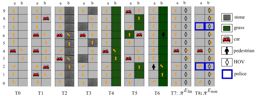
Fig. 2 illustrates a car driving simulator environment consisting of 999 different lane types (henceforth referred to as tasks), denoted as T0, T1, \ldots, T8. Each of these tasks is associated with different driving skills. For instance, task T0 corresponds to a basic setup representing a traffic-free highway—it has a very small probability of the presence of another car. However, task T1 represents a crowded highway with 0.250.250.25 probability of encountering a car. Task T2 has stones on the right lane, whereas task T3 has a mix of both cars and stones. Similarly, tasks T4 has grass on the right lane, and T5 has a mix of both grass and cars. Tasks T6, T7, and T8 introduce more complex features such as pedestrians, HOV, and police.
Refer to caption
Figure 1: Car environment with 999 different lane types (tasks). In any given lane, an agent starts from the bottom-left corner and the goal is to reach the top of the lane. Arrows represent the path taken by the teacher’s policy.
ϕ(s)italic-ϕ𝑠\phi(s) w𝑤w
stone -1
grass -0.5
car -5
ped -10
HOV -1
police 0
car-in-f -2
ped-in-f -5
Figure 2: ϕ(s)italic-ϕ𝑠\phi\left({s}\right) represents 888 features for a state s𝑠s. Weight vector w𝑤w is used to define the teacher’s reward function RElinsuperscript𝑅subscript𝐸linR^{E_{\mathrm{lin}}}.
Refer to caption
(a)
Refer to caption
(b)
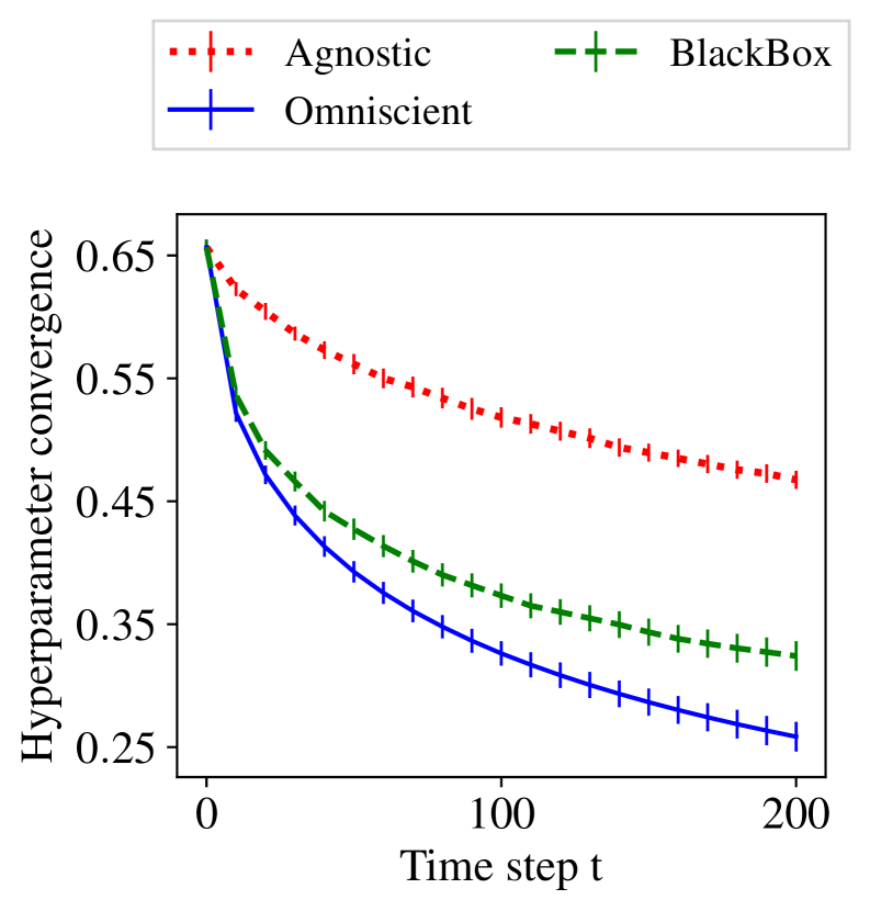
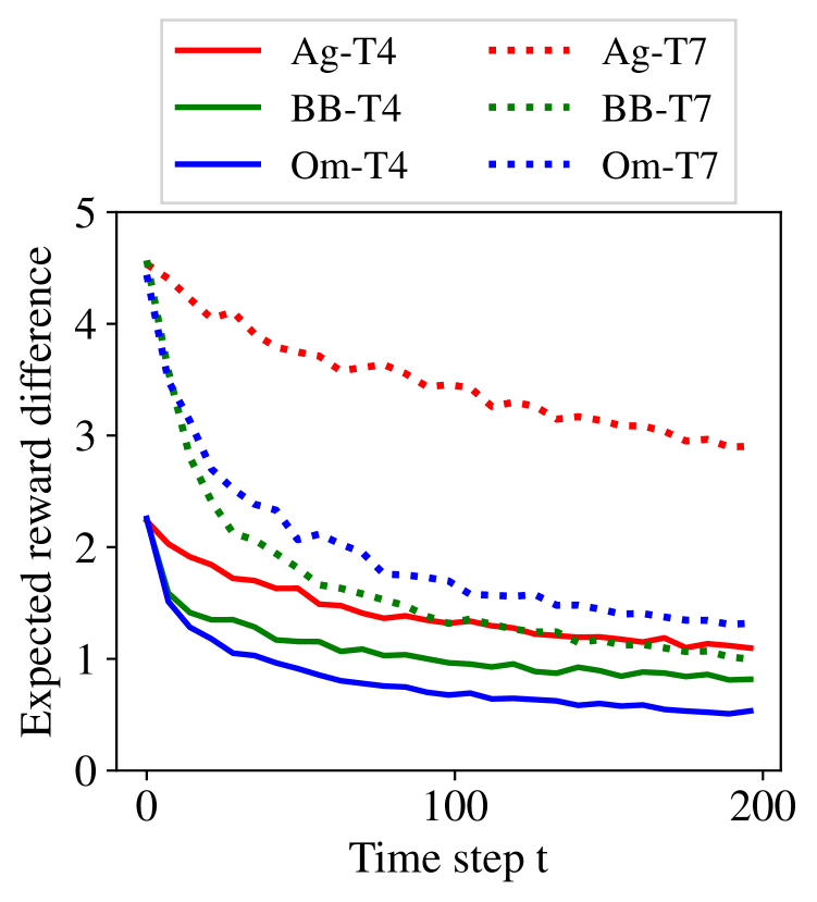
Figure 3: Linear setting of Section 6.1. (a) Convergence of the learner’s λtsubscript𝜆𝑡\lambda_{t} to the target λsuperscript𝜆\lambda^{*}. (b) Difference of total expected reward ν𝜈\nu of learner’s policy w.r.t. teacher’s policy in different tasks.
Refer to caption
(c)
Refer to caption
(d)
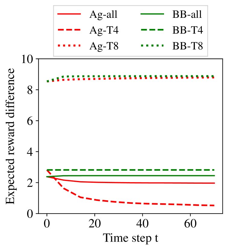
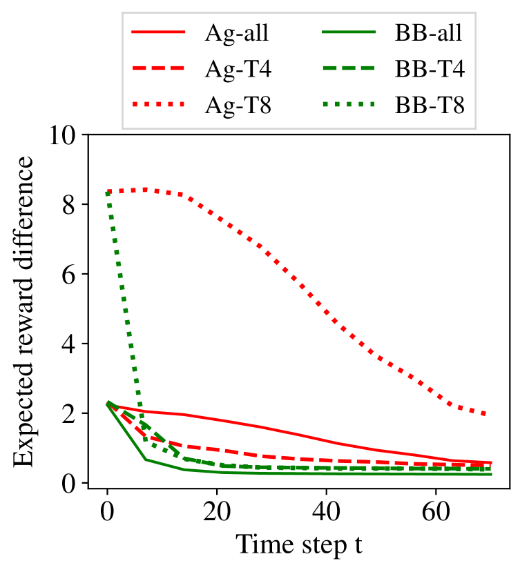
Figure 4: Non-linear setting of Section 6.2. (a) Results for a learner model with linear function RλLsubscriptsuperscript𝑅𝐿𝜆R^{L}_{\lambda} unable to represent the teacher’s reward. (b) Results for a learner model with non-linear function RλLsubscriptsuperscript𝑅𝐿𝜆R^{L}_{\lambda}.

The agent’s goal is to navigate starting from an initial state at the bottom left to the top of the lane. The agent can take three different actions given by 𝒜=𝒜absent\mathcal{A}= {left, straight, right}. Action left steers the agent to the left of the current lane. If agent is already in the leftmost lane when taking action left, then the lane is randomly chosen with probability 0.50.50.5. We define similar dynamics for taking action right; action straight means no change in the lane. Irrespective of the action taken, the agent always moves forward. W.l.o.g., we consider that only the agent moves in the environment.

6.1 Linear Reward Setting

First, we study a linear reward setting, and use the notation of linlin\mathrm{lin} in subscript to denote the MDP linsubscriptlin\mathcal{M}_{\mathrm{lin}}, the teacher’s reward RElinsuperscript𝑅subscript𝐸linR^{E_{\mathrm{lin}}}, and the teacher’s policy πElinsuperscript𝜋subscript𝐸lin\pi^{E_{\mathrm{lin}}}.

MDP.

We consider lanes corresponding to the first 888 tasks in the environment, namely T0, T1, \ldots, T7. We have n𝑛n number of lanes of a given task, each generated randomly according to the tasks’ characteristics described above. Hence, the total number of states |𝒮|𝒮\left|\mathcal{S}\right| in our MDP linsubscriptlin\mathcal{M}_{\mathrm{lin}} is n×8×20𝑛820n\times 8\times 20 where each cell represents a state, and each lane is associated with 202020 states (see Fig. 2). There is one initial state for each lane corresponding to the bottom left cell of that lane.

Teacher’s reward and policy.

Next, we define the reward function RElinsuperscript𝑅subscript𝐸linR^{E_{\mathrm{lin}}} (i.e., the teacher’s reward function). We consider a state-dependent reward that depends on the underlying features of a state s𝑠s given by the vector ϕ(s)italic-ϕ𝑠\phi\left({s}\right) as follows:

  • features indicating the type of the current grid cell as stone, grass, car, ped, HOV, and police.

  • features providing some look-ahead information such as whether there is a car or pedestrian in the immediate front cell (denoted as car-in-f and ped-in-f).

Given this, we define the teacher’s reward function of linear form as RElin(s)=w,ϕ(s)superscript𝑅subscript𝐸lin𝑠𝑤italic-ϕ𝑠R^{E_{\mathrm{lin}}}\left({s}\right)=\left\langle{w},{\phi\left({s}\right)}\right\rangle, where the w𝑤w values are given in Fig. 2. Teacher’s policy πElinsuperscript𝜋subscript𝐸lin\pi^{E_{\mathrm{lin}}} is then computed as the optimal policy w.r.t. this reward function and is illustrated via arrows in Fig. 2 (T0 to T7) representing the path taken by the teacher when driving in this environment.

Learner model.

We consider the learner model with linear reward function that depends only on state, i.e., RλL(s)=λ,ϕL(s)subscriptsuperscript𝑅𝐿𝜆𝑠𝜆superscriptitalic-ϕ𝐿𝑠R^{L}_{\lambda}\left({s}\right)=\left\langle{\lambda},{\phi^{L}\left({s}\right)}\right\rangle, where ϕL(s)=ϕ(s)superscriptitalic-ϕ𝐿𝑠italic-ϕ𝑠\phi^{L}\left({s}\right)=\phi\left({s}\right) as given in Fig. 2. The learner is implementing the sequential MCE-IRL in Algorithm 2, where the learner’s prior knowledge is captured by the initial policy π1Lsubscriptsuperscript𝜋𝐿1\pi^{L}_{1} (corresponding to hyperparameter λ1subscript𝜆1\lambda_{1}).

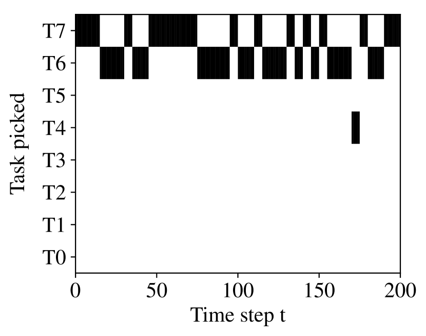
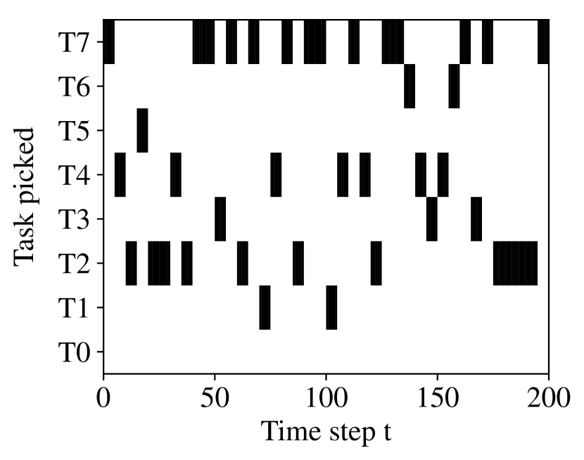
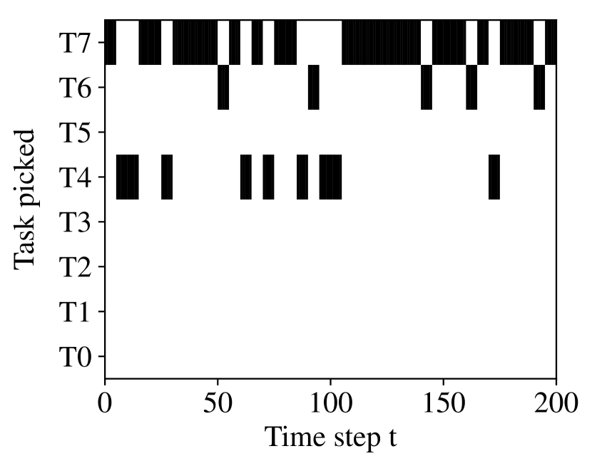
In the experiments, we consider the following prior knowledge of the learner: π1Lsubscriptsuperscript𝜋𝐿1\pi^{L}_{1} is initially trained based on demonstrations of πElinsuperscript𝜋subscript𝐸lin\pi^{E_{\mathrm{lin}}} sampled only from the lanes associated with the tasks T0, T1, T2, and T3. Intuitively, the learner initially possesses skills to avoid collisions with cars and to avoid hitting stones while driving. We expect to teach three major skills to the learner, i.e., avoiding grass while driving (task T4, T5, and T6), maintaining distance to pedestrians (task T6), and not to drive on HOV (task T7).
Refer to caption
(a) Learner’s initial skills: T0
Refer to caption
(b) Learner’s initial skills: T0T3
Refer to caption
(c) Learner’s inital skills: T0T5
Figure 5: Teaching curriculum (i.e., the task associated with the picked state st,0subscript𝑠𝑡0s_{t,0} by BboxTeacher in Algorithm 4) for three different settings depending on the learner’s initial skills trained on (a) T0, (b) T0T3, and (c) T0T5.

Experimental results.

We evaluate the performance of different teaching algorithms, and report the results by averaging over 101010 runs. We use n=5𝑛5n=5 lanes of each task (i.e., 404040 lanes in total). OmniTeacher in Algorithm 3 computes the target hyperparameter λsuperscript𝜆\lambda^{*} as per Footnote 5. For BboxTeacher in Algorithm 4, we use B=5𝐵5B=5 and k=5𝑘5k=5.

Fig. 3(a) shows the convergence of λtλ2subscriptdelimited-∥∥subscript𝜆𝑡superscript𝜆2\left\lVert\lambda_{t}-\lambda^{*}\right\rVert_{2}, where λsuperscript𝜆\lambda^{*} is computed by OmniTeacher. As expected, OmniTeacher outperforms other teaching algorithms (BboxTeacher and Agnostic teacher) that do not have knowledge of the learner’s dynamics and are not directly focusing on teaching this hyperparameter λsuperscript𝜆\lambda^{*}. Interestingly, the convergence of BboxTeacher is still significantly faster than Agnostic teacher. In Fig. 3(b), we consider the teaching objective of total expected reward difference |νπElinνπtL|superscript𝜈superscript𝜋subscript𝐸linsuperscript𝜈subscriptsuperscript𝜋𝐿𝑡|\nu^{\pi^{E_{\mathrm{lin}}}}-\nu^{\pi^{L}_{t}}|. We separately plot this objective with starting states limited to task T4 and task T7. The results suggest that convergence to target λsuperscript𝜆\lambda^{*} leads to reduction in expected reward difference (one of the teaching objective). The performance of BboxTeacher (BB-T7) is even better than OmniTeacher (Om-T7) for task T7. This is because BboxTeacher (Eq. (8)) picks tasks on which the learner’s total expected reward difference is highest.

Teaching curriculum.

In Fig. 5, we compare the teaching curriculum of BboxTeacher for three different settings, where the learner’s initial policy π1Lsubscriptsuperscript𝜋𝐿1\pi^{L}_{1} is trained based on demonstrations of πElinsuperscript𝜋subscript𝐸lin\pi^{E_{\mathrm{lin}}} sampled only from the lanes associated with the tasks (a) T0, (b) T0T3, and (c) T0T5. The curriculum here refers to the task associated with the state st,0subscript𝑠𝑡0s_{t,0} picked by the teacher at time t𝑡t to provide the demonstration. In these plots, we can see specific structures and temporal patterns emerging in the curriculum. In particular, we can see that the teaching curriculum focuses on tasks that help the learner acquire new skills. For instance, in Fig. 5(b), the teacher primarily picks tasks that provide new skills corresponding to the features grass, HOV, and ped. Recall that, for BboxTeacher (Algorithm 4), we use B=5𝐵5B=5 and k=5𝑘5k=5 for our experiments. As a result, the curriculum plots show blocks of length B=5𝐵5B=5 as the algorithm ends up picking the same task until new tests are performed to get a fresh estimate of the learner’s policy.

6.2 Non-linear Reward Setting

Here, we study a non-linear reward setting, and use the notation of nonnon\mathrm{non} in subscript for nonsubscriptnon\mathcal{M}_{\mathrm{non}}, REnonsuperscript𝑅subscript𝐸nonR^{E_{\mathrm{non}}}, and πEnonsuperscript𝜋subscript𝐸non\pi^{E_{\mathrm{non}}}.

MDP.

We consider the MDP nonsubscriptnon\mathcal{M}_{\mathrm{non}} which consists of lanes corresponding to 555 tasks: T0, T1, T2, T4, and T8 with the total number of states being n×5×20𝑛520n\times 5\times 20 as described above.

Teacher’s reward and policy.

Here, we define the teacher’s reward function REnonsuperscript𝑅subscript𝐸nonR^{E_{\mathrm{non}}}. The key difference between REnonsuperscript𝑅subscript𝐸nonR^{E_{\mathrm{non}}} and RElinsuperscript𝑅subscript𝐸linR^{E_{\mathrm{lin}}} is that the teacher in this setting prefers to drive on HOV (gets a +11+1 reward instead of 11-1 reward). However, if police is present while driving on HOV, there is a penalty of 55-5. Teacher’s optimal policy πEnonsuperscript𝜋subscript𝐸non\pi^{E_{\mathrm{non}}} for T8 is given in Fig. 2. For other tasks (apart from T7 and T8), the teacher’s optimal policy πEnonsuperscript𝜋subscript𝐸non\pi^{E_{\mathrm{non}}} is the same as πElinsuperscript𝜋subscript𝐸lin\pi^{E_{\mathrm{lin}}}.

Learner model.

We consider two different learner models: (i) with linear reward function RλL(s)=λ,ϕL(s)subscriptsuperscript𝑅𝐿𝜆𝑠𝜆superscriptitalic-ϕ𝐿𝑠R^{L}_{\lambda}\left({s}\right)=\left\langle{\lambda},{\phi^{L}\left({s}\right)}\right\rangle, and (ii) with non-linear reward function RλL(s)=λ1:d,ϕL(s)+λd+1:2d,ϕL(s)2subscriptsuperscript𝑅𝐿𝜆𝑠subscript𝜆:1superscript𝑑superscriptitalic-ϕ𝐿𝑠superscriptsubscript𝜆:superscript𝑑12superscript𝑑superscriptitalic-ϕ𝐿𝑠2R^{L}_{\lambda}\left({s}\right)=\left\langle{\lambda_{1:d^{\prime}}},{\phi^{L}\left({s}\right)}\right\rangle+{\left\langle{\lambda_{d^{\prime}+1:2d^{\prime}}},{\phi^{L}\left({s}\right)}\right\rangle}^{2}. Here, ϕL(s)=ϕ(s)superscriptitalic-ϕ𝐿𝑠italic-ϕ𝑠\phi^{L}\left({s}\right)=\phi\left({s}\right) as in Section 6.1 and d=8superscript𝑑8d^{\prime}=8 is the dimension of ϕ(s)italic-ϕ𝑠\phi\left({s}\right). As a prior knowledge to get π1Lsubscriptsuperscript𝜋𝐿1\pi^{L}_{1} at time t=1𝑡1t=1, we train the learner initially based on demonstrations of πEnonsuperscript𝜋subscript𝐸non\pi^{E_{\mathrm{non}}} sampled only from the lanes associated with the tasks T0, T1, and T2.

Experimental results.

We use similar experimental settings as in Section 6.1 (i.e., n=5𝑛5n=5, averaging 101010 runs, etc.). We separately report results for teaching a learner with linear RλLsubscriptsuperscript𝑅𝐿𝜆R^{L}_{\lambda} (see Fig. 3(c)) and non-linear RλLsubscriptsuperscript𝑅𝐿𝜆R^{L}_{\lambda} (see Fig. 3(d)).

Fig. 3(c) shows that both BboxTeacher and Agnostic teacher are unable to make progress in teaching task T8 to the learner. Interestingly, the overall performance measuring the total expected reward difference on the whole MDP for BboxTeacher (BB-all) is worse compared to Agnostic (Ag-all): This is an artifact of BboxTeacher’s strategy in Eq. (8) being stuck in always picking task T8 (even though the learner is not making any progress). Fig. 3(d) illustrates that the above mentioned limitations are gone when teaching a learner using a non-linear reward function. Here, the rate of reduction in total expected reward difference is significantly faster for BboxTeacher as compared to Agnostic, as was also observed in Fig. 3(b).

These results demonstrate that the learning progress can be sped up significantly by an adaptive teacher even with limited knowledge about the learner, as compared to an uninformative teacher. These results also signify the importance that the learner’s representation of feature space and reward function should be powerful enough to learn the desired behavior.

7 Related Work

Imitation learning.

The two popular approaches for imitation learning include (i) behavioral cloning, which directly replicates the desired behavior Bain and Sommut (1999), and (ii) inverse reinforcement learning (IRL) which infers the reward function explaining the desired behavior Russell (1998). We refer the reader to a recent survey by Osa et al. (2018) on imitation learning.

Amin et al. (2017) have studied interactive IRL algorithms that actively request the teacher to provide suitable demonstrations with the goal of reducing the number of interactions. However, the key difference in our approach is that we take the viewpoint of a teacher in how to best assist the learning agent by providing an optimal sequence of demonstrations. Our approach is inspired by real-life pedagogical settings where carefully choosing the teaching demonstrations and tasks can accelerate the learning progress Ho et al. (2016). Hadfield-Menell et al. (2016) have studied the value alignment problem in a game-theoretic setup, and provided an approximate scheme to generate instructive demonstrations for an IRL agent. In our work, we devise a systematic procedure (with convergence guarantees for the omniscient setting) to choose an optimal sequence of demonstrations, by taking into account the learner’s dynamics.

Steering and teaching in reinforcement learning.

A somewhat different but related problem setting is that of reward shaping and environment design where the goal is to modify/design the reward function to guide/steer the behavior of a learning agent Ng et al. (1999); Zhang et al. (2009); Sorg et al. (2010). Another related problem setting is considered in the advice-based interaction framework (e.g., Torrey and Taylor (2013); Amir et al. (2016)), where the goal is to communicate advice to a suboptimal agent on how to act in the world.

Algorithmic teaching.

Another line of research relevant to our work is that of algorithmic teaching. Here, one studies the interaction between a teacher and a learner where the teacher’s objective is to find an optimal training sequence to steer the learner towards a desired goal Goldman and Kearns (1995); Liu et al. (2017); Zhu et al. (2018). Algorithmic teaching provides a rigorous formalism for a number of real-world applications such as personalized education and intelligent tutoring systems Patil et al. (2014); Rafferty et al. (2016); Hunziker et al. (2018), social robotics Cakmak and Thomaz (2014), and human-in-the-loop systems Singla et al. (2014, 2013). Most of the work in machine teaching is in a batch setting where the teacher provides a batch of teaching examples at once without any adaptation. The question of how a teacher should adaptively select teaching examples for a learner has been addressed recently but only in the supervised learning setting Melo et al. (2018); Liu et al. (2018); Chen et al. (2018); Yeo et al. (2019).

Teaching sequential tasks.

Walsh and Goschin (2012); Cakmak and Lopes (2012) have studied algorithmic teaching for sequential decision-making tasks. Cakmak and Lopes (2012) studied the problem of teaching an IRL agent in the batch setting, i.e., the teacher has to provide a near-optimal set of demonstrations at once. They considered the IRL algorithm by Ng and Russell (2000), which could only result in inferring an equivalent class of reward weight parameters for which the observed behavior is optimal. In recent work, Brown and Niekum (2019) have extended the previous work of Cakmak and Lopes (2012) by showing that the teaching problem can be formulated as a set cover problem. However, their teaching strategy does not take into account how the learner progresses (i.e., it is non-interactive). In contrast, we study interactive teaching setting to teach a sequential MCE-IRL algorithm Ziebart et al. (2008); Rhinehart and Kitani (2017). This interactive setting, in turn, allows the teacher to design a personalized and adaptive curriculum important for efficient learning Tadepalli (2008). Haug et al. (2018) have studied the problem of teaching an IRL agent adaptively; however, they consider a very different setting where the teacher and the learner have a mismatch in their worldviews.

8 Conclusions

We studied the problem of designing interactive teaching algorithms to provide an informative sequence of demonstrations to a sequential IRL learner. In an omniscient teaching setting, we presented OmniTeacher which achieves the teaching objective with 𝒪(log1ϵ)𝒪1italic-ϵ\mathcal{O}\left({\log\frac{1}{\epsilon}}\right) demonstrations. Then, utilizing the insights from OmniTeacher, we proposed BboxTeacher for a more practical blackbox setting. We showed the effectiveness of our algorithms via extensive experiments in a learning environment inspired by a car driving simulator.

As future work, we will investigate extensions of our ideas to more complex environments; we hope that, ultimately, such extensions will provide a basis for designing teaching strategies for intelligent tutoring systems (see Footnote 1 and Footnote 2). It would also be interesting to benchmark active imitation methods for MCE-IRL learner using our omniscient teacher (see, e.g., Brown and Niekum (2019)). Our results are also important in getting a better understanding of the robustness of MCE-IRL learner against adversarial training-set poisoning attacks. Our fast convergence results in Theorem 1 suggests that the MCE-IRL learner is actually brittle to adversarial attacks, and designing a robust MCE-IRL is an important direction of future work.

Acknowledgments. This work was supported in part by the Swiss National Science Foundation (SNSF) under grant number 407540_167319.

References

  • Abbeel and Ng (2004) Pieter Abbeel and Andrew Y Ng. Apprenticeship learning via inverse reinforcement learning. In ICML, 2004.
  • Amin et al. (2017) Kareem Amin, Nan Jiang, and Satinder P. Singh. Repeated inverse reinforcement learning. In NIPS, pages 1813–1822, 2017.
  • Amir et al. (2016) Ofra Amir, Ece Kamar, Andrey Kolobov, and Barbara J. Grosz. Interactive teaching strategies for agent training. In IJCAI, pages 804–811, 2016.
  • Argall et al. (2009) Brenna D Argall, Sonia Chernova, Manuela Veloso, and Brett Browning. A survey of robot learning from demonstration. Robotics and autonomous systems, 2009.
  • Bain and Sommut (1999) Michael Bain and Claude Sommut. A framework for hehavioural claning. Machine Intelligence 15, 15:103, 1999.
  • Billard et al. (2008) Aude Billard, Sylvain Calinon, Ruediger Dillmann, and Stefan Schaal. Robot programming by demonstration. In Springer handbook of robotics. 2008.
  • Boularias et al. (2011) Abdeslam Boularias, Jens Kober, and Jan Peters. Relative entropy inverse reinforcement learning. In AISTATS, pages 182–189, 2011.
  • Brown and Niekum (2019) Daniel S. Brown and Scott Niekum. Machine teaching for inverse reinforcement learning: Algorithms and applications. In AAAI, 2019.
  • Buchsbaum et al. (2011) Daphna Buchsbaum, Alison Gopnik, Thomas L Griffiths, and Patrick Shafto. Children’s imitation of causal action sequences is influenced by statistical and pedagogical evidence. Cognition, 2011.
  • Cakmak and Lopes (2012) Maya Cakmak and Manuel Lopes. Algorithmic and human teaching of sequential decision tasks. In AAAI, 2012.
  • Cakmak and Thomaz (2014) Maya Cakmak and Andrea L Thomaz. Eliciting good teaching from humans for machine learners. Artificial Intelligence, 217:198–215, 2014.
  • Chen et al. (2018) Yuxin Chen, Adish Singla, Oisin Mac Aodha, Pietro Perona, and Yisong Yue. Understanding the role of adaptivity in machine teaching: The case of version space learners. In NeurIPS, 2018.
  • Chernova and Thomaz (2014) Sonia Chernova and Andrea L Thomaz. Robot learning from human teachers. Synthesis Lectures on Artificial Intelligence and Machine Learning, 2014.
  • Dorsa Sadigh et al. (2017) Anca D Dragan Dorsa Sadigh, Shankar Sastry, and Sanjit A Seshia. Active preference-based learning of reward functions. In RSS, 2017.
  • Finn et al. (2016) Chelsea Finn, Sergey Levine, and Pieter Abbeel. Guided cost learning: Deep inverse optimal control via policy optimization. In ICML, pages 49–58, 2016.
  • Goldman and Kearns (1995) Sally A Goldman and Michael J Kearns. On the complexity of teaching. Journal of Computer and System Sciences, 50(1):20–31, 1995.
  • Hadfield-Menell et al. (2016) Dylan Hadfield-Menell, Stuart J Russell, Pieter Abbeel, and Anca Dragan. Cooperative inverse reinforcement learning. In NIPS, 2016.
  • Haug et al. (2018) Luis Haug, Sebastian Tschiatschek, and Adish Singla. Teaching Inverse Reinforcement Learners via Features and Demonstrations. In NeurIPS, 2018.
  • Ho and Ermon (2016) Jonathan Ho and Stefano Ermon. Generative adversarial imitation learning. In NIPS, 2016.
  • Ho et al. (2016) Mark K Ho, Michael Littman, James MacGlashan, Fiery Cushman, and Joseph L Austerweil. Showing versus doing: Teaching by demonstration. In NIPS, 2016.
  • Hunziker et al. (2018) Anette Hunziker, Yuxin Chen, Oisin Mac Aodha, Manuel Gomez-Rodriguez, Andreas Krause, Pietro Perona, Yisong Yue, and Adish Singla. Teaching multiple concepts to a forgetful learner. CoRR, abs/1805.08322, 2018.
  • Levine et al. (2010) Sergey Levine, Zoran Popovic, and Vladlen Koltun. Feature construction for inverse reinforcement learning. In NIPS, pages 1342–1350, 2010.
  • Liu et al. (2017) Weiyang Liu, Bo Dai, Ahmad Humayun, Charlene Tay, Chen Yu, Linda B. Smith, James M. Rehg, and Le Song. Iterative machine teaching. In ICML, 2017.
  • Liu et al. (2018) Weiyang Liu, Bo Dai, Xingguo Li, Zhen Liu, James Rehg, and Le Song. Towards black-box iterative machine teaching. In ICML, 2018.
  • Melo et al. (2018) Francisco S Melo, Carla Guerra, and Manuel Lopes. Interactive optimal teaching with unknown learners. In IJCAI, pages 2567–2573, 2018.
  • Ng and Russell (2000) Andrew Y Ng and Stuart J Russell. Algorithms for inverse reinforcement learning. In ICML, 2000.
  • Ng et al. (1999) Andrew Y Ng, Daishi Harada, and Stuart Russell. Policy invariance under reward transformations: Theory and application to reward shaping. In ICML, 1999.
  • Osa et al. (2018) Takayuki Osa, Joni Pajarinen, Gerhard Neumann, J Andrew Bagnell, Pieter Abbeel, Jan Peters, et al. An algorithmic perspective on imitation learning. Foundations and Trends® in Robotics, 7(1-2):1–179, 2018.
  • Patil et al. (2014) Kaustubh R Patil, Xiaojin Zhu, Łukasz Kopeć, and Bradley C Love. Optimal teaching for limited-capacity human learners. In NIPS, pages 2465–2473, 2014.
  • Rafferty et al. (2016) Anna N Rafferty, Emma Brunskill, Thomas L Griffiths, and Patrick Shafto. Faster teaching via pomdp planning. Cognitive science, 2016.
  • Ratliff et al. (2006) Nathan D Ratliff, J Andrew Bagnell, and Martin A Zinkevich. Maximum margin planning. In ICML, pages 729–736, 2006.
  • Rhinehart and Kitani (2017) Nicholas Rhinehart and Kris M Kitani. First-person activity forecasting with online inverse reinforcement learning. In ICCV, pages 3696–3705, 2017.
  • Russell (1998) Stuart Russell. Learning agents for uncertain environments. In COLT, pages 101–103, 1998.
  • Schaal (1997) Stefan Schaal. Learning from demonstration. In NIPS, pages 1040–1046, 1997.
  • Shafto et al. (2014) Patrick Shafto, Noah D Goodman, and Thomas L Griffiths. A rational account of pedagogical reasoning: Teaching by, and learning from, examples. Cognitive psychology, 71:55–89, 2014.
  • Singla et al. (2013) Adish Singla, Ilija Bogunovic, G Bartók, A Karbasi, and A Krause. On actively teaching the crowd to classify. In NIPS Workshop on Data Driven Education, 2013.
  • Singla et al. (2014) Adish Singla, Ilija Bogunovic, Gábor Bartók, Amin Karbasi, and Andreas Krause. Near-optimally teaching the crowd to classify. In ICML, 2014.
  • Sorg et al. (2010) Jonathan Sorg, Satinder P. Singh, and Richard L. Lewis. Reward design via online gradient ascent. In NIPS, pages 2190–2198, 2010.
  • Sun et al. (2018) Wen Sun, Geoffrey J Gordon, Byron Boots, and J Andrew Bagnell. Dual policy iteration. arXiv:1805.10755, 2018.
  • Tadepalli (2008) Prasad Tadepalli. Learning to solve problems from exercises. Computational Intelligence, 2008.
  • Torrey and Taylor (2013) Lisa Torrey and Matthew Taylor. Teaching on a budget: Agents advising agents in reinforcement learning. In AAMAS, pages 1053–1060, 2013.
  • Walsh and Goschin (2012) Thomas J. Walsh and Sergiu Goschin. Dynamic teaching in sequential decision making environments. In UAI, 2012.
  • Wulfmeier et al. (2015) Markus Wulfmeier, Peter Ondruska, and Ingmar Posner. Maximum entropy deep inverse reinforcement learning. CoRR, abs/1507.04888, 2015.
  • Yeo et al. (2019) Teresa Yeo, Parameswaran Kamalaruban, Adish Singla, Arpit Merchant, Thibault Asselborn, Louis Faucon, Pierre Dillenbourg, and Volkan Cevher. Iterative classroom teaching. In AAAI, 2019.
  • Zhang et al. (2009) Haoqi Zhang, David C Parkes, and Yiling Chen. Policy teaching through reward function learning. In EC, pages 295–304, 2009.
  • Zhou et al. (2018) Zhengyuan Zhou, Michael Bloem, and Nicholas Bambos. Infinite time horizon maximum causal entropy inverse reinforcement learning. IEEE Trans. Automat. Contr., 63(9):2787–2802, 2018.
  • Zhu et al. (2018) Xiaojin Zhu, Adish Singla, Sandra Zilles, and Anna N. Rafferty. An overview of machine teaching. CoRR, abs/1801.05927, 2018.
  • Ziebart et al. (2008) Brian D Ziebart, Andrew L Maas, J Andrew Bagnell, and Anind K Dey. Maximum entropy inverse reinforcement learning. In AAAI, 2008.
  • Ziebart (2010) Brian D Ziebart. Modeling purposeful adaptive behavior with the principle of maximum causal entropy. Carnegie Mellon University, 2010.

Appendix A Gradient for Sequential MCE-IRL

In this section, we show that gtsubscript𝑔𝑡g_{t} can be seen as an empirical counterpart of the gradient of the following loss function:

c(λ;πE)=𝔼{(sτ,aτ)}τ(πE,)[τγτlogπλL(aτsτ)]𝑐𝜆superscript𝜋𝐸similar-tosubscriptsubscript𝑠𝜏subscript𝑎𝜏𝜏superscript𝜋𝐸𝔼delimited-[]subscript𝜏superscript𝛾𝜏subscriptsuperscript𝜋𝐿𝜆conditionalsubscript𝑎𝜏subscript𝑠𝜏c\left({\lambda;\pi^{E}}\right)~{}=~{}\underset{\left\{{\left({s_{\tau},a_{\tau}}\right)}\right\}_{\tau}\sim\left({\pi^{E},\mathcal{M}}\right)}{\mathbb{E}}\left[{-\sum_{\tau}\gamma^{\tau}\log\pi^{L}_{\lambda}\left({a_{\tau}\mid s_{\tau}}\right)}\right]

capturing the discounted negative log-likelihood of teacher’s demonstrations. In Proposition 1, we show that gradient λc(λ;πE)subscript𝜆𝑐𝜆superscript𝜋𝐸\nabla_{\lambda}c\left({\lambda;\pi^{E}}\right) is given by s,a[ρπλL(s,a)ρπE(s,a)]λRλL(s,a)subscript𝑠𝑎delimited-[]superscript𝜌subscriptsuperscript𝜋𝐿𝜆𝑠𝑎superscript𝜌superscript𝜋𝐸𝑠𝑎subscript𝜆subscriptsuperscript𝑅𝐿𝜆𝑠𝑎\sum_{s,a}\left[{\rho^{\pi^{L}_{\lambda}}\left({s,a}\right)-\rho^{\pi^{E}}\left({s,a}\right)}\right]\nabla_{\lambda}R^{L}_{\lambda}\left({s,a}\right) (see Eq. (9)).

Given the teacher’s demonstration ξtsubscript𝜉𝑡\xi_{t} with starting state st,0subscript𝑠𝑡0s_{t,0}, we compute gtsubscript𝑔𝑡g_{t} as follows:

  • In Eq. (9), consider the gradient component corresponding to teacher’s policy, i.e., s,aρπE(s,a)λRλL(s,a)subscript𝑠𝑎superscript𝜌superscript𝜋𝐸𝑠𝑎subscript𝜆subscriptsuperscript𝑅𝐿𝜆𝑠𝑎-\sum_{s,a}\rho^{\pi^{E}}\left({s,a}\right)\nabla_{\lambda}R^{L}_{\lambda}\left({s,a}\right). We replace ρπE(s,a)superscript𝜌superscript𝜋𝐸𝑠𝑎\rho^{\pi^{E}}\left({s,a}\right) with it’s empirical counterpart using ξtsubscript𝜉𝑡\xi_{t}. This results in the following component in gtsubscript𝑔𝑡g_{t}:

    s,aρξt(s,a)λRλL(s,a)|λ=λtevaluated-atsubscript𝑠𝑎superscript𝜌subscript𝜉𝑡𝑠𝑎subscript𝜆subscriptsuperscript𝑅𝐿𝜆𝑠𝑎𝜆subscript𝜆𝑡-\sum_{s,a}\rho^{\xi_{t}}\left({s,a}\right)\nabla_{\lambda}R^{L}_{\lambda}\left({s,a}\right)\big{|}_{\lambda=\lambda_{t}}
  • In Eq. (9), consider the gradient component corresponding to learner’s policy, i.e., s,aρπλL(s,a)λRλL(s,a)subscript𝑠𝑎superscript𝜌subscriptsuperscript𝜋𝐿𝜆𝑠𝑎subscript𝜆subscriptsuperscript𝑅𝐿𝜆𝑠𝑎\sum_{s,a}\rho^{\pi^{L}_{\lambda}}\left({s,a}\right)\nabla_{\lambda}R^{L}_{\lambda}\left({s,a}\right). We compute ρπλL(s,a)superscript𝜌subscriptsuperscript𝜋𝐿𝜆𝑠𝑎\rho^{\pi^{L}_{\lambda}}\left({s,a}\right) with st,0subscript𝑠𝑡0s_{t,0} as the only initial state, i.e., P0(st,0)=1subscript𝑃0subscript𝑠𝑡01P_{0}(s_{t,0})=1. This results in the following component in gtsubscript𝑔𝑡g_{t}:

    s,aρπtL,st,0(s,a)λRλL(s,a)|λ=λtevaluated-atsubscript𝑠𝑎superscript𝜌subscriptsuperscript𝜋𝐿𝑡subscript𝑠𝑡0𝑠𝑎subscript𝜆subscriptsuperscript𝑅𝐿𝜆𝑠𝑎𝜆subscript𝜆𝑡\sum_{s,a}\rho^{\pi^{L}_{t},s_{t,0}}\left({s,a}\right)\nabla_{\lambda}R^{L}_{\lambda}\left({s,a}\right)\big{|}_{\lambda=\lambda_{t}}

Hence, gtsubscript𝑔𝑡g_{t} given by

gt=s,a[ρπtL,st,0(s,a)ρξt(s,a)]λRλL(s,a)|λ=λt.subscript𝑔𝑡evaluated-atsubscript𝑠𝑎delimited-[]superscript𝜌subscriptsuperscript𝜋𝐿𝑡subscript𝑠𝑡0𝑠𝑎superscript𝜌subscript𝜉𝑡𝑠𝑎subscript𝜆subscriptsuperscript𝑅𝐿𝜆𝑠𝑎𝜆subscript𝜆𝑡g_{t}~{}=~{}\sum_{s,a}\left[{\rho^{\pi^{L}_{t},s_{t,0}}\left({s,a}\right)-\rho^{\xi_{t}}\left({s,a}\right)}\right]\nabla_{\lambda}R^{L}_{\lambda}\left({s,a}\right)\big{|}_{\lambda=\lambda_{t}}.
Proposition 1.

Consider the loss function defined as follows:

c(λ;πE):=𝔼{(sτ,aτ)}τ(πE,)[τγτlogπλL(aτsτ)].assign𝑐𝜆superscript𝜋𝐸similar-tosubscriptsubscript𝑠𝜏subscript𝑎𝜏𝜏superscript𝜋𝐸𝔼delimited-[]subscript𝜏superscript𝛾𝜏subscriptsuperscript𝜋𝐿𝜆conditionalsubscript𝑎𝜏subscript𝑠𝜏c\left({\lambda;\pi^{E}}\right)~{}:=~{}\underset{\left\{{\left({s_{\tau},a_{\tau}}\right)}\right\}_{\tau}\sim\left({\pi^{E},\mathcal{M}}\right)}{\mathbb{E}}\left[{-\sum_{\tau}\gamma^{\tau}\log\pi^{L}_{\lambda}\left({a_{\tau}\mid s_{\tau}}\right)}\right].

Then the gradient of c(λ;πE)𝑐𝜆superscript𝜋𝐸c\left({\lambda;\pi^{E}}\right) w.r.t. λ𝜆\lambda is given by

λc(λ;πE)=s,a[ρπλL(s,a)ρπE(s,a)]λRλL(s,a).subscript𝜆𝑐𝜆superscript𝜋𝐸subscript𝑠𝑎delimited-[]superscript𝜌subscriptsuperscript𝜋𝐿𝜆𝑠𝑎superscript𝜌superscript𝜋𝐸𝑠𝑎subscript𝜆subscriptsuperscript𝑅𝐿𝜆𝑠𝑎\nabla_{\lambda}c\left({\lambda;\pi^{E}}\right)~{}=~{}\sum_{s,a}\left[{\rho^{\pi^{L}_{\lambda}}\left({s,a}\right)-\rho^{\pi^{E}}\left({s,a}\right)}\right]\nabla_{\lambda}R^{L}_{\lambda}\left({s,a}\right). (9)
Proof.

We will make use of the following quantities as part of the proof:

  • PτL(s)subscriptsuperscript𝑃𝐿𝜏𝑠P^{L}_{\tau}\left({s}\right) is defined as the probability of visiting state s𝑠s at time τ𝜏\tau by the policy πλLsubscriptsuperscript𝜋𝐿𝜆\pi^{L}_{\lambda}.

  • PτL(s,a)subscriptsuperscript𝑃𝐿𝜏𝑠𝑎P^{L}_{\tau}\left({s,a}\right) is defined as the probability of taking action a𝑎a from state s𝑠s at time τ𝜏\tau by the policy πλLsubscriptsuperscript𝜋𝐿𝜆\pi^{L}_{\lambda}.

  • PτE(s)subscriptsuperscript𝑃𝐸𝜏𝑠P^{E}_{\tau}\left({s}\right) is defined as the probability of visiting state s𝑠s at time τ𝜏\tau by the policy πEsuperscript𝜋𝐸\pi^{E}.

  • PτE(s,a)subscriptsuperscript𝑃𝐸𝜏𝑠𝑎P^{E}_{\tau}\left({s,a}\right) is defined as the probability of taking action a𝑎a from state s𝑠s at time τ𝜏\tau by the policy πEsuperscript𝜋𝐸\pi^{E}.

First, we rewrite c(λ;πE)𝑐𝜆superscript𝜋𝐸c\left({\lambda;\pi^{E}}\right) as follows:

c(λ;πE)=𝑐𝜆superscript𝜋𝐸absent\displaystyle c\left({\lambda;\pi^{E}}\right)~{}=~{} τ=0s,aPτE(s)PτE(as)γτ[Qλ(s,a)Vλ(s)]superscriptsubscript𝜏0subscript𝑠𝑎subscriptsuperscript𝑃𝐸𝜏𝑠subscriptsuperscript𝑃𝐸𝜏conditional𝑎𝑠superscript𝛾𝜏delimited-[]subscript𝑄𝜆𝑠𝑎subscript𝑉𝜆𝑠\displaystyle-\sum_{\tau=0}^{\infty}\sum_{s,a}P^{E}_{\tau}\left({s}\right)P^{E}_{\tau}\left({a\mid s}\right)\gamma^{\tau}\left[{Q_{\lambda}\left({s,a}\right)-V_{\lambda}\left({s}\right)}\right]
=\displaystyle~{}=~{} s,aP0(s)P0E(as)[Qλ(s,a)Vλ(s)]subscript𝑠𝑎subscript𝑃0𝑠subscriptsuperscript𝑃𝐸0conditional𝑎𝑠delimited-[]subscript𝑄𝜆𝑠𝑎subscript𝑉𝜆𝑠\displaystyle-\sum_{s,a}P_{0}\left({s}\right)P^{E}_{0}\left({a\mid s}\right)\left[{Q_{\lambda}\left({s,a}\right)-V_{\lambda}\left({s}\right)}\right]
s,aP1E(s)P1E(as)γ[Qλ(s,a)Vλ(s)]subscript𝑠𝑎subscriptsuperscript𝑃𝐸1𝑠subscriptsuperscript𝑃𝐸1conditional𝑎𝑠𝛾delimited-[]subscript𝑄𝜆𝑠𝑎subscript𝑉𝜆𝑠\displaystyle-\sum_{s,a}P^{E}_{1}\left({s}\right)P^{E}_{1}\left({a\mid s}\right)\gamma\left[{Q_{\lambda}\left({s,a}\right)-V_{\lambda}\left({s}\right)}\right]
s,aP2E(s)P2E(as)γ2[Qλ(s,a)Vλ(s)]subscript𝑠𝑎subscriptsuperscript𝑃𝐸2𝑠subscriptsuperscript𝑃𝐸2conditional𝑎𝑠superscript𝛾2delimited-[]subscript𝑄𝜆𝑠𝑎subscript𝑉𝜆𝑠\displaystyle-\sum_{s,a}P^{E}_{2}\left({s}\right)P^{E}_{2}\left({a\mid s}\right)\gamma^{2}\left[{Q_{\lambda}\left({s,a}\right)-V_{\lambda}\left({s}\right)}\right]
s,aP3E(s)P3E(as)γ3[Qλ(s,a)Vλ(s)]subscript𝑠𝑎subscriptsuperscript𝑃𝐸3𝑠subscriptsuperscript𝑃𝐸3conditional𝑎𝑠superscript𝛾3delimited-[]subscript𝑄𝜆𝑠𝑎subscript𝑉𝜆𝑠\displaystyle-\sum_{s,a}P^{E}_{3}\left({s}\right)P^{E}_{3}\left({a\mid s}\right)\gamma^{3}\left[{Q_{\lambda}\left({s,a}\right)-V_{\lambda}\left({s}\right)}\right]
\displaystyle\dots
=\displaystyle~{}=~{} s,aP0(s)P0E(as)Vλ(s)subscript𝑠𝑎subscript𝑃0𝑠subscriptsuperscript𝑃𝐸0conditional𝑎𝑠subscript𝑉𝜆𝑠\displaystyle\sum_{s,a}P_{0}\left({s}\right)P^{E}_{0}\left({a\mid s}\right)V_{\lambda}\left({s}\right)
s,aP0(s)P0E(as)Qλ(s,a)+γs,aP1E(s)P1E(as)Vλ(s)subscript𝑠𝑎subscript𝑃0𝑠subscriptsuperscript𝑃𝐸0conditional𝑎𝑠subscript𝑄𝜆𝑠𝑎𝛾subscript𝑠𝑎subscriptsuperscript𝑃𝐸1𝑠subscriptsuperscript𝑃𝐸1conditional𝑎𝑠subscript𝑉𝜆𝑠\displaystyle-\sum_{s,a}P_{0}\left({s}\right)P^{E}_{0}\left({a\mid s}\right)Q_{\lambda}\left({s,a}\right)+\gamma\sum_{s,a}P^{E}_{1}\left({s}\right)P^{E}_{1}\left({a\mid s}\right)V_{\lambda}\left({s}\right)
γs,aP1E(s)P1E(as)Qλ(s,a)+γ2s,aP2E(s)P2E(as)Vλ(s)𝛾subscript𝑠𝑎subscriptsuperscript𝑃𝐸1𝑠subscriptsuperscript𝑃𝐸1conditional𝑎𝑠subscript𝑄𝜆𝑠𝑎superscript𝛾2subscript𝑠𝑎subscriptsuperscript𝑃𝐸2𝑠subscriptsuperscript𝑃𝐸2conditional𝑎𝑠subscript𝑉𝜆𝑠\displaystyle-\gamma\sum_{s,a}P^{E}_{1}\left({s}\right)P^{E}_{1}\left({a\mid s}\right)Q_{\lambda}\left({s,a}\right)+\gamma^{2}\sum_{s,a}P^{E}_{2}\left({s}\right)P^{E}_{2}\left({a\mid s}\right)V_{\lambda}\left({s}\right)
γ2s,aP2E(s)P2E(as)Qλ(s,a)+γ3s,aP3E(s)P3E(as)Vλ(s)superscript𝛾2subscript𝑠𝑎subscriptsuperscript𝑃𝐸2𝑠subscriptsuperscript𝑃𝐸2conditional𝑎𝑠subscript𝑄𝜆𝑠𝑎superscript𝛾3subscript𝑠𝑎subscriptsuperscript𝑃𝐸3𝑠subscriptsuperscript𝑃𝐸3conditional𝑎𝑠subscript𝑉𝜆𝑠\displaystyle-\gamma^{2}\sum_{s,a}P^{E}_{2}\left({s}\right)P^{E}_{2}\left({a\mid s}\right)Q_{\lambda}\left({s,a}\right)+\gamma^{3}\sum_{s,a}P^{E}_{3}\left({s}\right)P^{E}_{3}\left({a\mid s}\right)V_{\lambda}\left({s}\right)
\displaystyle\dots
=\displaystyle~{}=~{} sP0(s)Vλ(s)subscript𝑠subscript𝑃0𝑠subscript𝑉𝜆𝑠\displaystyle{\color[rgb]{1,0,0}\definecolor[named]{pgfstrokecolor}{rgb}{1,0,0}\sum_{s}P_{0}\left({s}\right)V_{\lambda}\left({s}\right)}
s,aP0E(s,a)Qλ(s,a)+γsP1E(s)Vλ(s)subscript𝑠𝑎subscriptsuperscript𝑃𝐸0𝑠𝑎subscript𝑄𝜆𝑠𝑎𝛾subscript𝑠subscriptsuperscript𝑃𝐸1𝑠subscript𝑉𝜆𝑠\displaystyle{\color[rgb]{0,0,1}\definecolor[named]{pgfstrokecolor}{rgb}{0,0,1}-\sum_{s,a}P^{E}_{0}\left({s,a}\right)Q_{\lambda}\left({s,a}\right)+\gamma\sum_{s}P^{E}_{1}\left({s}\right)V_{\lambda}\left({s}\right)}
γs,aP1E(s,a)Qλ(s,a)+γ2sP2E(s)Vλ(s)𝛾subscript𝑠𝑎subscriptsuperscript𝑃𝐸1𝑠𝑎subscript𝑄𝜆𝑠𝑎superscript𝛾2subscript𝑠subscriptsuperscript𝑃𝐸2𝑠subscript𝑉𝜆𝑠\displaystyle{\color[rgb]{1,0,1}\definecolor[named]{pgfstrokecolor}{rgb}{1,0,1}\pgfsys@color@cmyk@stroke{0}{1}{0}{0}\pgfsys@color@cmyk@fill{0}{1}{0}{0}-\gamma\sum_{s,a}P^{E}_{1}\left({s,a}\right)Q_{\lambda}\left({s,a}\right)+\gamma^{2}\sum_{s}P^{E}_{2}\left({s}\right)V_{\lambda}\left({s}\right)}
γ2s,aP2E(s,a)Qλ(s,a)+γ3sP3E(s)Vλ(s)superscript𝛾2subscript𝑠𝑎subscriptsuperscript𝑃𝐸2𝑠𝑎subscript𝑄𝜆𝑠𝑎superscript𝛾3subscript𝑠subscriptsuperscript𝑃𝐸3𝑠subscript𝑉𝜆𝑠\displaystyle{\color[rgb]{.5,0,.5}\definecolor[named]{pgfstrokecolor}{rgb}{.5,0,.5}-\gamma^{2}\sum_{s,a}P^{E}_{2}\left({s,a}\right)Q_{\lambda}\left({s,a}\right)+\gamma^{3}\sum_{s}P^{E}_{3}\left({s}\right)V_{\lambda}\left({s}\right)}
\displaystyle\dots

Now, we compute the gradient of the first term:

λsP0(s)Vλ(s)=subscript𝜆subscript𝑠subscript𝑃0𝑠subscript𝑉𝜆𝑠absent\displaystyle\nabla_{\lambda}\sum_{s}P_{0}\left({s}\right)V_{\lambda}\left({s}\right)~{}=~{} sP0(s)λVλ(s)subscript𝑠subscript𝑃0𝑠subscript𝜆subscript𝑉𝜆𝑠\displaystyle\sum_{s}P_{0}\left({s}\right)\nabla_{\lambda}V_{\lambda}\left({s}\right)
=\displaystyle~{}=~{} sP0(s)λlogaexp(Qλ(s,a))subscript𝑠subscript𝑃0𝑠subscript𝜆subscript𝑎subscript𝑄𝜆𝑠𝑎\displaystyle\sum_{s}P_{0}\left({s}\right)\nabla_{\lambda}\log\sum_{a}{\exp\left({Q_{\lambda}\left({s,a}\right)}\right)}
=\displaystyle~{}=~{} sP0(s)aexp(Qλ(s,a))λQλ(s,a)aexp(Qλ(s,a))subscript𝑠subscript𝑃0𝑠subscript𝑎subscript𝑄𝜆𝑠𝑎subscript𝜆subscript𝑄𝜆𝑠𝑎subscript𝑎subscript𝑄𝜆𝑠𝑎\displaystyle\sum_{s}P_{0}\left({s}\right)\frac{\sum_{a}{\exp\left({Q_{\lambda}\left({s,a}\right)}\right)\nabla_{\lambda}Q_{\lambda}\left({s,a}\right)}}{\sum_{a}{\exp\left({Q_{\lambda}\left({s,a}\right)}\right)}}
=\displaystyle~{}=~{} sP0(s)aπλL(as)λQλ(s,a)subscript𝑠subscript𝑃0𝑠subscript𝑎subscriptsuperscript𝜋𝐿𝜆conditional𝑎𝑠subscript𝜆subscript𝑄𝜆𝑠𝑎\displaystyle\sum_{s}P_{0}\left({s}\right)\sum_{a}\pi^{L}_{\lambda}(a\mid s)\nabla_{\lambda}Q_{\lambda}\left({s,a}\right)
=\displaystyle~{}=~{} s,aP0L(s,a)[λRλL(s,a)+γsT(ss,a)λVλ(s)]subscript𝑠𝑎subscriptsuperscript𝑃𝐿0𝑠𝑎delimited-[]subscript𝜆subscriptsuperscript𝑅𝐿𝜆𝑠𝑎𝛾subscriptsuperscript𝑠𝑇conditionalsuperscript𝑠𝑠𝑎subscript𝜆subscript𝑉𝜆superscript𝑠\displaystyle\sum_{s,a}P^{L}_{0}\left({s,a}\right)\left[{\nabla_{\lambda}R^{L}_{\lambda}\left({s,a}\right)+\gamma\sum_{s^{\prime}}{T(s^{\prime}\mid s,a)\nabla_{\lambda}V_{\lambda}\left({s^{\prime}}\right)}}\right]
=\displaystyle~{}=~{} s,aP0L(s,a)λRλL(s,a)+ss,aP0L(s,a)T(ss,a)γλVλ(s)subscript𝑠𝑎subscriptsuperscript𝑃𝐿0𝑠𝑎subscript𝜆subscriptsuperscript𝑅𝐿𝜆𝑠𝑎subscriptsuperscript𝑠subscript𝑠𝑎subscriptsuperscript𝑃𝐿0𝑠𝑎𝑇conditionalsuperscript𝑠𝑠𝑎𝛾subscript𝜆subscript𝑉𝜆superscript𝑠\displaystyle\sum_{s,a}P^{L}_{0}\left({s,a}\right)\nabla_{\lambda}R^{L}_{\lambda}\left({s,a}\right)+\sum_{s^{\prime}}\sum_{s,a}P^{L}_{0}\left({s,a}\right)T(s^{\prime}\mid s,a)\gamma\nabla_{\lambda}V_{\lambda}\left({s^{\prime}}\right)
=\displaystyle~{}=~{} s,aP0L(s,a)λRλL(s,a)+sP1L(s)γλVλ(s)subscript𝑠𝑎subscriptsuperscript𝑃𝐿0𝑠𝑎subscript𝜆subscriptsuperscript𝑅𝐿𝜆𝑠𝑎subscriptsuperscript𝑠subscriptsuperscript𝑃𝐿1superscript𝑠𝛾subscript𝜆subscript𝑉𝜆superscript𝑠\displaystyle\sum_{s,a}P^{L}_{0}\left({s,a}\right)\nabla_{\lambda}R^{L}_{\lambda}\left({s,a}\right)+\sum_{s^{\prime}}P^{L}_{1}\left({s^{\prime}}\right)\gamma\nabla_{\lambda}V_{\lambda}\left({s^{\prime}}\right)
=\displaystyle~{}=~{} s,aP0L(s,a)λRλL(s,a)+s,aP1L(s,a)γλRλL(s,a)+sP2L(s)γ2λVλ(s)subscript𝑠𝑎subscriptsuperscript𝑃𝐿0𝑠𝑎subscript𝜆subscriptsuperscript𝑅𝐿𝜆𝑠𝑎subscript𝑠𝑎subscriptsuperscript𝑃𝐿1𝑠𝑎𝛾subscript𝜆subscriptsuperscript𝑅𝐿𝜆𝑠𝑎subscriptsuperscript𝑠subscriptsuperscript𝑃𝐿2superscript𝑠superscript𝛾2subscript𝜆subscript𝑉𝜆superscript𝑠\displaystyle\sum_{s,a}P^{L}_{0}\left({s,a}\right)\nabla_{\lambda}R^{L}_{\lambda}\left({s,a}\right)+\sum_{s,a}P^{L}_{1}\left({s,a}\right)\gamma\nabla_{\lambda}R^{L}_{\lambda}\left({s,a}\right)+\sum_{s^{\prime}}P^{L}_{2}\left({s^{\prime}}\right)\gamma^{2}\nabla_{\lambda}V_{\lambda}\left({s^{\prime}}\right)
\displaystyle\vdots
=\displaystyle~{}=~{} s,aρπλL(s,a)λRλL(s,a).subscript𝑠𝑎superscript𝜌subscriptsuperscript𝜋𝐿𝜆𝑠𝑎subscript𝜆subscriptsuperscript𝑅𝐿𝜆𝑠𝑎\displaystyle\sum_{s,a}\rho^{\pi^{L}_{\lambda}}\left({s,a}\right)\nabla_{\lambda}R^{L}_{\lambda}\left({s,a}\right).

Now, we compute the gradient of the second term:

s,aP0E(s,a)λQλ(s,a)+γsP1E(s)λVλ(s)subscript𝑠𝑎subscriptsuperscript𝑃𝐸0𝑠𝑎subscript𝜆subscript𝑄𝜆𝑠𝑎𝛾subscript𝑠subscriptsuperscript𝑃𝐸1𝑠subscript𝜆subscript𝑉𝜆𝑠\displaystyle-\sum_{s,a}P^{E}_{0}\left({s,a}\right)\nabla_{\lambda}Q_{\lambda}\left({s,a}\right)+\gamma\sum_{s}P^{E}_{1}\left({s}\right)\nabla_{\lambda}V_{\lambda}\left({s}\right)
=\displaystyle~{}=~{} s,aP0E(s,a)[λRλL(s,a)+γsT(ss,a)λVλ(s)]+γsP1E(s)λVλ(s)subscript𝑠𝑎subscriptsuperscript𝑃𝐸0𝑠𝑎delimited-[]subscript𝜆subscriptsuperscript𝑅𝐿𝜆𝑠𝑎𝛾subscriptsuperscript𝑠𝑇conditionalsuperscript𝑠𝑠𝑎subscript𝜆subscript𝑉𝜆superscript𝑠𝛾subscript𝑠subscriptsuperscript𝑃𝐸1𝑠subscript𝜆subscript𝑉𝜆𝑠\displaystyle-\sum_{s,a}P^{E}_{0}\left({s,a}\right)\left[{\nabla_{\lambda}R^{L}_{\lambda}\left({s,a}\right)+\gamma\sum_{s^{\prime}}{T(s^{\prime}\mid s,a)\nabla_{\lambda}V_{\lambda}\left({s^{\prime}}\right)}}\right]+\gamma\sum_{s}P^{E}_{1}\left({s}\right)\nabla_{\lambda}V_{\lambda}\left({s}\right)
=\displaystyle~{}=~{} s,aP0E(s,a)λRλL(s,a)γss,aP0E(s,a)T(ss,a)λVλ(s)+γsP1E(s)λVλ(s)subscript𝑠𝑎subscriptsuperscript𝑃𝐸0𝑠𝑎subscript𝜆subscriptsuperscript𝑅𝐿𝜆𝑠𝑎𝛾subscriptsuperscript𝑠subscript𝑠𝑎subscriptsuperscript𝑃𝐸0𝑠𝑎𝑇conditionalsuperscript𝑠𝑠𝑎subscript𝜆subscript𝑉𝜆superscript𝑠𝛾subscript𝑠subscriptsuperscript𝑃𝐸1𝑠subscript𝜆subscript𝑉𝜆𝑠\displaystyle-\sum_{s,a}P^{E}_{0}\left({s,a}\right)\nabla_{\lambda}R^{L}_{\lambda}\left({s,a}\right)-\gamma\sum_{s^{\prime}}\sum_{s,a}P^{E}_{0}\left({s,a}\right)T(s^{\prime}\mid s,a)\nabla_{\lambda}V_{\lambda}\left({s^{\prime}}\right)+\gamma\sum_{s}P^{E}_{1}\left({s}\right)\nabla_{\lambda}V_{\lambda}\left({s}\right)
=\displaystyle~{}=~{} s,aP0E(s,a)λRλL(s,a)γsP1E(s)λVλ(s)+γsP1E(s)λVλ(s)subscript𝑠𝑎subscriptsuperscript𝑃𝐸0𝑠𝑎subscript𝜆subscriptsuperscript𝑅𝐿𝜆𝑠𝑎𝛾subscriptsuperscript𝑠subscriptsuperscript𝑃𝐸1superscript𝑠subscript𝜆subscript𝑉𝜆superscript𝑠𝛾subscript𝑠subscriptsuperscript𝑃𝐸1𝑠subscript𝜆subscript𝑉𝜆𝑠\displaystyle-\sum_{s,a}P^{E}_{0}\left({s,a}\right)\nabla_{\lambda}R^{L}_{\lambda}\left({s,a}\right)-\gamma\sum_{s^{\prime}}P^{E}_{1}\left({s^{\prime}}\right)\nabla_{\lambda}V_{\lambda}\left({s^{\prime}}\right)+\gamma\sum_{s}P^{E}_{1}\left({s}\right)\nabla_{\lambda}V_{\lambda}\left({s}\right)
=\displaystyle~{}=~{} s,aP0E(s,a)λRλL(s,a).subscript𝑠𝑎subscriptsuperscript𝑃𝐸0𝑠𝑎subscript𝜆subscriptsuperscript𝑅𝐿𝜆𝑠𝑎\displaystyle-\sum_{s,a}P^{E}_{0}\left({s,a}\right)\nabla_{\lambda}R^{L}_{\lambda}\left({s,a}\right).

By following similar steps, the gradient of all the terms except the first term is given by

τ=0s,aPτE(s,a)γτλRλL(s,a)=s,aρπE(s,a)λRλL(s,a).superscriptsubscript𝜏0subscript𝑠𝑎subscriptsuperscript𝑃𝐸𝜏𝑠𝑎superscript𝛾𝜏subscript𝜆subscriptsuperscript𝑅𝐿𝜆𝑠𝑎subscript𝑠𝑎superscript𝜌superscript𝜋𝐸𝑠𝑎subscript𝜆subscriptsuperscript𝑅𝐿𝜆𝑠𝑎-\sum_{\tau=0}^{\infty}\sum_{s,a}P^{E}_{\tau}\left({s,a}\right)\gamma^{\tau}\nabla_{\lambda}R^{L}_{\lambda}\left({s,a}\right)~{}=~{}-\sum_{s,a}\rho^{\pi^{E}}\left({s,a}\right)\nabla_{\lambda}R^{L}_{\lambda}\left({s,a}\right).

Thus the full gradient is given by

λc(λ;πE)=s,a[ρπλL(s,a)ρπE(s,a)]λRλL(s,a).subscript𝜆𝑐𝜆superscript𝜋𝐸subscript𝑠𝑎delimited-[]superscript𝜌subscriptsuperscript𝜋𝐿𝜆𝑠𝑎superscript𝜌superscript𝜋𝐸𝑠𝑎subscript𝜆subscriptsuperscript𝑅𝐿𝜆𝑠𝑎\nabla_{\lambda}c\left({\lambda;\pi^{E}}\right)~{}=~{}\sum_{s,a}\left[{\rho^{\pi^{L}_{\lambda}}\left({s,a}\right)-\rho^{\pi^{E}}\left({s,a}\right)}\right]\nabla_{\lambda}R^{L}_{\lambda}\left({s,a}\right).

Appendix B Proofs

In this section, we provide proofs of Lemma 1 and Lemma 2.

B.1 Proof of Lemma 1

Proof.

The demonstration ξtsubscript𝜉𝑡\xi_{t} (starting from st,0subscript𝑠𝑡0s_{t,0}) provided by the teacher at time t𝑡t satisfies the following:

μξt=μπtL,st,0βt(λtλ)+δt,superscript𝜇subscript𝜉𝑡superscript𝜇subscriptsuperscript𝜋𝐿𝑡subscript𝑠𝑡0subscript𝛽𝑡subscript𝜆𝑡superscript𝜆subscript𝛿𝑡\mu^{\xi_{t}}~{}=~{}\mu^{\pi^{L}_{t},s_{t,0}}-\beta_{t}\left({\lambda_{t}-\lambda^{*}}\right)+\delta_{t}, (10)

for some δtsubscript𝛿𝑡\delta_{t} s.t. δt2Δmaxsubscriptdelimited-∥∥subscript𝛿𝑡2subscriptΔmax\left\lVert\delta_{t}\right\rVert_{2}\leq\Delta_{\mathrm{max}}, and βt[0,1ηt]subscript𝛽𝑡01subscript𝜂𝑡\beta_{t}\in\left[{0,\frac{1}{\eta_{t}}}\right]. Consider:

λt+1λ2=superscriptdelimited-∥∥subscript𝜆𝑡1superscript𝜆2absent\displaystyle\left\lVert\lambda_{t+1}-\lambda^{*}\right\rVert^{2}~{}=~{} ΠΩ[λtηt(μπtL,st,0μξt)]λ2superscriptdelimited-∥∥subscriptΠΩdelimited-[]subscript𝜆𝑡subscript𝜂𝑡superscript𝜇subscriptsuperscript𝜋𝐿𝑡subscript𝑠𝑡0superscript𝜇subscript𝜉𝑡superscript𝜆2\displaystyle\left\lVert\Pi_{\Omega}\left[{\lambda_{t}-\eta_{t}(\mu^{\pi^{L}_{t},s_{t,0}}-\mu^{\xi_{t}})}\right]-\lambda^{*}\right\rVert^{2}
(i)𝑖\displaystyle~{}\overset{(i)}{\leq}~{} λtηt(μπtL,st,0μξt)λ2superscriptdelimited-∥∥subscript𝜆𝑡subscript𝜂𝑡superscript𝜇subscriptsuperscript𝜋𝐿𝑡subscript𝑠𝑡0superscript𝜇subscript𝜉𝑡superscript𝜆2\displaystyle\left\lVert\lambda_{t}-\eta_{t}\left({\mu^{\pi^{L}_{t},s_{t,0}}-\mu^{\xi_{t}}}\right)-\lambda^{*}\right\rVert^{2}
=\displaystyle~{}=~{} λtλ22ηtλtλ,μπtL,st,0μξt+ηt2μπtL,st,0μξt2superscriptdelimited-∥∥subscript𝜆𝑡superscript𝜆22subscript𝜂𝑡subscript𝜆𝑡superscript𝜆superscript𝜇subscriptsuperscript𝜋𝐿𝑡subscript𝑠𝑡0superscript𝜇subscript𝜉𝑡superscriptsubscript𝜂𝑡2superscriptdelimited-∥∥superscript𝜇subscriptsuperscript𝜋𝐿𝑡subscript𝑠𝑡0superscript𝜇subscript𝜉𝑡2\displaystyle\left\lVert\lambda_{t}-\lambda^{*}\right\rVert^{2}-2\eta_{t}\left\langle{\lambda_{t}-\lambda^{*}},{\mu^{\pi^{L}_{t},s_{t,0}}-\mu^{\xi_{t}}}\right\rangle+\eta_{t}^{2}\left\lVert\mu^{\pi^{L}_{t},s_{t,0}}-\mu^{\xi_{t}}\right\rVert^{2}
=(ii)𝑖𝑖\displaystyle~{}\overset{(ii)}{=}~{} λtλ22ηtλtλ,βt(λtλ)δt+ηt2βt(λtλ)δt2superscriptdelimited-∥∥subscript𝜆𝑡superscript𝜆22subscript𝜂𝑡subscript𝜆𝑡superscript𝜆subscript𝛽𝑡subscript𝜆𝑡superscript𝜆subscript𝛿𝑡superscriptsubscript𝜂𝑡2superscriptdelimited-∥∥subscript𝛽𝑡subscript𝜆𝑡superscript𝜆subscript𝛿𝑡2\displaystyle\left\lVert\lambda_{t}-\lambda^{*}\right\rVert^{2}-2\eta_{t}\left\langle{\lambda_{t}-\lambda^{*}},{\beta_{t}\left({\lambda_{t}-\lambda^{*}}\right)-\delta_{t}}\right\rangle+\eta_{t}^{2}\left\lVert\beta_{t}\left({\lambda_{t}-\lambda^{*}}\right)-\delta_{t}\right\rVert^{2}
=\displaystyle~{}=~{} λtλ22ηtβtλtλ,λtλ+ηt2βt2λtλ2superscriptdelimited-∥∥subscript𝜆𝑡superscript𝜆22subscript𝜂𝑡subscript𝛽𝑡subscript𝜆𝑡superscript𝜆subscript𝜆𝑡superscript𝜆superscriptsubscript𝜂𝑡2superscriptsubscript𝛽𝑡2superscriptdelimited-∥∥subscript𝜆𝑡superscript𝜆2\displaystyle\left\lVert\lambda_{t}-\lambda^{*}\right\rVert^{2}-2\eta_{t}\beta_{t}\left\langle{\lambda_{t}-\lambda^{*}},{\lambda_{t}-\lambda^{*}}\right\rangle+\eta_{t}^{2}\beta_{t}^{2}\left\lVert\lambda_{t}-\lambda^{*}\right\rVert^{2}
+2ηtλtλ,δt+ηt2δt22ηt2βtλtλ,δt2subscript𝜂𝑡subscript𝜆𝑡superscript𝜆subscript𝛿𝑡superscriptsubscript𝜂𝑡2superscriptdelimited-∥∥subscript𝛿𝑡22superscriptsubscript𝜂𝑡2subscript𝛽𝑡subscript𝜆𝑡superscript𝜆subscript𝛿𝑡\displaystyle+2\eta_{t}\left\langle{\lambda_{t}-\lambda^{*}},{\delta_{t}}\right\rangle+\eta_{t}^{2}\left\lVert\delta_{t}\right\rVert^{2}-2\eta_{t}^{2}\beta_{t}\left\langle{\lambda_{t}-\lambda^{*}},{\delta_{t}}\right\rangle
=\displaystyle~{}=~{} (1ηtβt)2λtλ2+2ηt(1ηtβt)λtλ,δt+ηt2δt2superscript1subscript𝜂𝑡subscript𝛽𝑡2superscriptdelimited-∥∥subscript𝜆𝑡superscript𝜆22subscript𝜂𝑡1subscript𝜂𝑡subscript𝛽𝑡subscript𝜆𝑡superscript𝜆subscript𝛿𝑡superscriptsubscript𝜂𝑡2superscriptdelimited-∥∥subscript𝛿𝑡2\displaystyle\left({1-\eta_{t}\beta_{t}}\right)^{2}\left\lVert\lambda_{t}-\lambda^{*}\right\rVert^{2}+2\eta_{t}(1-\eta_{t}\beta_{t})\left\langle{\lambda_{t}-\lambda^{*}},{\delta_{t}}\right\rangle+\eta_{t}^{2}\left\lVert\delta_{t}\right\rVert^{2}
(iii)𝑖𝑖𝑖\displaystyle~{}\overset{(iii)}{\leq}~{} (1ηtβt)2λtλ2+2ηt(1ηtβt)λtλδt+ηt2δt2superscript1subscript𝜂𝑡subscript𝛽𝑡2superscriptdelimited-∥∥subscript𝜆𝑡superscript𝜆22subscript𝜂𝑡1subscript𝜂𝑡subscript𝛽𝑡delimited-∥∥subscript𝜆𝑡superscript𝜆delimited-∥∥subscript𝛿𝑡superscriptsubscript𝜂𝑡2superscriptdelimited-∥∥subscript𝛿𝑡2\displaystyle\left({1-\eta_{t}\beta_{t}}\right)^{2}\left\lVert\lambda_{t}-\lambda^{*}\right\rVert^{2}+2\eta_{t}(1-\eta_{t}\beta_{t})\left\lVert\lambda_{t}-\lambda^{*}\right\rVert\left\lVert\delta_{t}\right\rVert+\eta_{t}^{2}\left\lVert\delta_{t}\right\rVert^{2}
(iv)𝑖𝑣\displaystyle~{}\overset{(iv)}{\leq}~{} (1β)2λtλ2+2ηt(1β)λtλδt+ηtδtsuperscript1𝛽2superscriptdelimited-∥∥subscript𝜆𝑡superscript𝜆22subscript𝜂𝑡1𝛽delimited-∥∥subscript𝜆𝑡superscript𝜆delimited-∥∥subscript𝛿𝑡subscript𝜂𝑡delimited-∥∥subscript𝛿𝑡\displaystyle\left({1-\beta}\right)^{2}\left\lVert\lambda_{t}-\lambda^{*}\right\rVert^{2}+2\eta_{t}(1-\beta)\left\lVert\lambda_{t}-\lambda^{*}\right\rVert\left\lVert\delta_{t}\right\rVert+\eta_{t}\left\lVert\delta_{t}\right\rVert
(v)𝑣\displaystyle~{}\overset{(v)}{\leq}~{} (1β)2λtλ2+4ηt(1β)zδt+ηtδtsuperscript1𝛽2superscriptdelimited-∥∥subscript𝜆𝑡superscript𝜆24subscript𝜂𝑡1𝛽𝑧delimited-∥∥subscript𝛿𝑡subscript𝜂𝑡delimited-∥∥subscript𝛿𝑡\displaystyle\left({1-\beta}\right)^{2}\left\lVert\lambda_{t}-\lambda^{*}\right\rVert^{2}+4\eta_{t}(1-\beta)z\left\lVert\delta_{t}\right\rVert+\eta_{t}\left\lVert\delta_{t}\right\rVert
\displaystyle~{}\leq~{} (1β)2λtλ2+ηmax[4(1β)z+1]Δmax,superscript1𝛽2superscriptdelimited-∥∥subscript𝜆𝑡superscript𝜆2subscript𝜂maxdelimited-[]41𝛽𝑧1subscriptΔmax\displaystyle\left({1-\beta}\right)^{2}\left\lVert\lambda_{t}-\lambda^{*}\right\rVert^{2}+\eta_{\mathrm{max}}\left[{4(1-\beta)z+1}\right]\Delta_{\mathrm{max}},

where (i)𝑖(i) is by the property of projection, (ii)𝑖𝑖(ii) is by applying Eq. (10), (iii)𝑖𝑖𝑖(iii) is due to Cauchy–Schwarz inequality, (iv)𝑖𝑣(iv) is by definition β=mintηtβt𝛽subscript𝑡subscript𝜂𝑡subscript𝛽𝑡\beta=\min_{t}\eta_{t}\beta_{t}, and (v)𝑣(v) is due to the fact λΩ={λ:λ2z}𝜆Ωconditional-set𝜆subscriptdelimited-∥∥𝜆2𝑧\lambda\in\Omega=\left\{{\lambda:\left\lVert\lambda\right\rVert_{2}\leq z}\right\}.

By using the fact that a+ba+b𝑎𝑏𝑎𝑏\sqrt{a+b}\leq\sqrt{a}+\sqrt{b} for all positive a,b𝑎𝑏a,b (and by recurrence), we have:

λt+1λdelimited-∥∥subscript𝜆𝑡1superscript𝜆absent\displaystyle\left\lVert\lambda_{t+1}-\lambda^{*}\right\rVert~{}\leq~{} (1β)λtλ+ηmax[4(1β)z+1]Δmax1𝛽delimited-∥∥subscript𝜆𝑡superscript𝜆subscript𝜂maxdelimited-[]41𝛽𝑧1subscriptΔmax\displaystyle\left({1-\beta}\right)\left\lVert\lambda_{t}-\lambda^{*}\right\rVert+\sqrt{\eta_{\mathrm{max}}\left[{4(1-\beta)z+1}\right]\Delta_{\mathrm{max}}}
\displaystyle~{}\leq~{} (1β)tλ1λ+ηmax[4(1β)z+1]Δmaxs=0(1β)ssuperscript1𝛽𝑡delimited-∥∥subscript𝜆1superscript𝜆subscript𝜂maxdelimited-[]41𝛽𝑧1subscriptΔmaxsuperscriptsubscript𝑠0superscript1𝛽𝑠\displaystyle\left({1-\beta}\right)^{t}\left\lVert\lambda_{1}-\lambda^{*}\right\rVert+\sqrt{\eta_{\mathrm{max}}\left[{4(1-\beta)z+1}\right]\Delta_{\mathrm{max}}}\sum_{s=0}^{\infty}{\left({1-\beta}\right)^{s}}
\displaystyle~{}\leq~{} (1β)tλ1λ+ηmax[4(1β)z+1]Δmax1βsuperscript1𝛽𝑡delimited-∥∥subscript𝜆1superscript𝜆subscript𝜂maxdelimited-[]41𝛽𝑧1subscriptΔmax1𝛽\displaystyle\left({1-\beta}\right)^{t}\left\lVert\lambda_{1}-\lambda^{*}\right\rVert+\sqrt{\eta_{\mathrm{max}}\left[{4(1-\beta)z+1}\right]\Delta_{\mathrm{max}}}\cdot\frac{1}{\beta}
\displaystyle~{}\leq~{} ϵ2+ϵ2=ϵ,superscriptitalic-ϵ2superscriptitalic-ϵ2superscriptitalic-ϵ\displaystyle\frac{\epsilon^{\prime}}{2}+\frac{\epsilon^{\prime}}{2}~{}=~{}\epsilon^{\prime},

for t=(log11β)1log2λ1λϵ𝑡superscript11𝛽12delimited-∥∥subscript𝜆1superscript𝜆superscriptitalic-ϵt=\left({\log\frac{1}{1-\beta}}\right)^{-1}\log\frac{2\left\lVert\lambda_{1}-\lambda^{*}\right\rVert}{\epsilon^{\prime}}, and Δmax=ϵ2β24ηmax[4(1β)z+1]subscriptΔmaxsuperscriptsuperscriptitalic-ϵ2superscript𝛽24subscript𝜂maxdelimited-[]41𝛽𝑧1\Delta_{\mathrm{max}}=\frac{{\epsilon^{\prime}}^{2}\beta^{2}}{4\eta_{\mathrm{max}}\left[{4(1-\beta)z+1}\right]}. ∎

B.2 Proof of Lemma 2

Proof.

We use the following inequalities in the proof:

  • Pinsker’s inequality: If P𝑃P and Q𝑄Q are two probability distributions on a measurable space, then

    DTV(P,Q)2DKL(P,Q)subscript𝐷TV𝑃𝑄2subscript𝐷KL𝑃𝑄D_{\mathrm{TV}}(P,Q)~{}\leq~{}\sqrt{2D_{\mathrm{KL}}(P,Q)} (11)
  • Log-sum inequality: For non-negative a1,a2,ansubscript𝑎1subscript𝑎2subscript𝑎𝑛a_{1},a_{2}...,a_{n} and b1,b2,bnsubscript𝑏1subscript𝑏2subscript𝑏𝑛b_{1},b_{2}...,b_{n} we have:

    i=1nailogaibi(i=1nai)logi=1naii=1nbisuperscriptsubscript𝑖1𝑛subscript𝑎𝑖subscript𝑎𝑖subscript𝑏𝑖superscriptsubscript𝑖1𝑛subscript𝑎𝑖superscriptsubscript𝑖1𝑛subscript𝑎𝑖superscriptsubscript𝑖1𝑛subscript𝑏𝑖\sum_{i=1}^{n}a_{i}\log\frac{a_{i}}{b_{i}}~{}\geq~{}\left(\sum_{i=1}^{n}a_{i}\right)\log\frac{\sum_{i=1}^{n}a_{i}}{\sum_{i=1}^{n}b_{i}} (12)
  • For any two policy π𝜋\pi and πsuperscript𝜋\pi^{\prime} (acting in the MDP \mathcal{M}), we have [Sun et al., 2018, Lemma A.1]:

    DTV(ρπ,ρπ)21γmaxsDTV(π(|s),π(|s)),D_{\mathrm{TV}}(\rho^{\pi},\rho^{\pi^{\prime}})~{}\leq~{}\frac{2}{1-\gamma}\cdot\max_{s}D_{\mathrm{TV}}(\pi(\cdot|s),\pi^{\prime}(\cdot|s)), (13)

    where DTV(p,q):=x|p(x)q(x)|assignsubscript𝐷TV𝑝𝑞subscript𝑥𝑝𝑥𝑞𝑥D_{\mathrm{TV}}(p,q):=\sum_{x}\left|p(x)-q(x)\right| is the TV-divergence between two distributions p𝑝p and q𝑞q. This implies that “similar" policies behave “similarly" in the MDP.

Then due to (13), and Pinsker’s inequality (11), we have:

DTV(ρπλL,ρπλL)subscript𝐷TVsuperscript𝜌subscriptsuperscript𝜋𝐿𝜆superscript𝜌subscriptsuperscript𝜋𝐿superscript𝜆absent\displaystyle D_{\mathrm{TV}}\left({\rho^{\pi^{L}_{\lambda}},\rho^{\pi^{L}_{\lambda^{\prime}}}}\right)~{}\leq~{} 21γmaxsDTV(πλL(|s),πλL(|s))\displaystyle\frac{2}{1-\gamma}\cdot\max_{s}D_{\mathrm{TV}}\left({\pi^{L}_{\lambda}(\cdot|s),\pi^{L}_{\lambda^{\prime}}(\cdot|s)}\right)
\displaystyle~{}\leq~{} 21γ2maxsDKL(πλL(|s),πλL(|s)).\displaystyle\frac{2}{1-\gamma}\cdot\sqrt{2\max_{s}D_{\mathrm{KL}}\left({\pi^{L}_{\lambda}(\cdot|s),\pi^{L}_{\lambda^{\prime}}(\cdot|s)}\right)}. (14)

The soft Bellman policy associated with the parameter λ𝜆\lambda is given by:

πλL(as)=subscriptsuperscript𝜋𝐿𝜆conditional𝑎𝑠absent\displaystyle\pi^{L}_{\lambda}(a\mid s)~{}=~{} Zas,λZs,λsubscript𝑍conditional𝑎𝑠𝜆subscript𝑍𝑠𝜆\displaystyle\frac{Z_{a\mid s,\lambda}}{Z_{s,\lambda}}
logZs,λ=subscript𝑍𝑠𝜆absent\displaystyle\log Z_{s,\lambda}~{}=~{} logaZas,λsubscript𝑎subscript𝑍conditional𝑎𝑠𝜆\displaystyle\log\sum_{a}{Z_{a\mid s,\lambda}}
logZas,λ=subscript𝑍conditional𝑎𝑠𝜆absent\displaystyle\log Z_{a\mid s,\lambda}~{}=~{} RλL(s,a)+γsT(ss,a)logZs,λ.subscriptsuperscript𝑅𝐿𝜆𝑠𝑎𝛾subscriptsuperscript𝑠𝑇conditionalsuperscript𝑠𝑠𝑎subscript𝑍superscript𝑠𝜆\displaystyle R^{L}_{\lambda}\left({s,a}\right)+\gamma\sum_{s^{\prime}}{T(s^{\prime}\mid s,a)\log Z_{s^{\prime},\lambda}}. (15)

Consider for any state s𝑠s:

DKL(πλL(|s),πλL(|s))=aπλL(a|s){logZas,λZas,λ+logZs,λZs,λ}\displaystyle D_{\mathrm{KL}}(\pi^{L}_{\lambda}(\cdot|s),\pi^{L}_{\lambda^{\prime}}(\cdot|s))=\sum_{a}{\pi^{L}_{\lambda}(a|s)\left\{{\log\frac{Z_{a\mid s,\lambda}}{Z_{a\mid s,\lambda^{\prime}}}+\log\frac{Z_{s,\lambda^{\prime}}}{Z_{s,\lambda}}}\right\}}
=(aπλL(a|s)logZas,λZas,λ)+logZs,λZs,λ,absentsubscript𝑎subscriptsuperscript𝜋𝐿𝜆conditional𝑎𝑠subscript𝑍conditional𝑎𝑠𝜆subscript𝑍conditional𝑎𝑠superscript𝜆subscript𝑍𝑠superscript𝜆subscript𝑍𝑠𝜆\displaystyle=\left(\sum_{a}\pi^{L}_{\lambda}(a|s)\log\frac{Z_{a\mid s,\lambda}}{Z_{a\mid s,\lambda^{\prime}}}\right)+\log\frac{Z_{s,\lambda^{\prime}}}{Z_{s,\lambda}}, (16)

where the first equation is by the definition of DKLsubscript𝐷KLD_{\mathrm{KL}}, and second is due to the fact that aπλL(a|s)=1subscript𝑎subscriptsuperscript𝜋𝐿𝜆conditional𝑎𝑠1\sum_{a}\pi^{L}_{\lambda}(a|s)=1. By using log-sum inequality (12) we have:

logZs,λZs,λ=subscript𝑍𝑠superscript𝜆subscript𝑍𝑠𝜆absent\displaystyle\log\frac{Z_{s,\lambda^{\prime}}}{Z_{s,\lambda}}~{}=~{} 1Zs,λaZa|s,λ=1logaZa|s,λaZa|s,λ\displaystyle\underbrace{\frac{1}{Z_{s,\lambda^{\prime}}}\cdot\sum_{a}{Z_{a|s,\lambda^{\prime}}\cdot}}_{=1}\log\frac{\sum_{a}Z_{a|s,\lambda^{\prime}}}{\sum_{a}Z_{a|s,\lambda}}
\displaystyle~{}\leq~{} 1Zs,λaZa|s,λlogZa|s,λZa|s,λ1subscript𝑍𝑠superscript𝜆subscript𝑎subscript𝑍conditional𝑎𝑠superscript𝜆subscript𝑍conditional𝑎𝑠superscript𝜆subscript𝑍conditional𝑎𝑠𝜆\displaystyle\frac{1}{Z_{s,\lambda^{\prime}}}\sum_{a}{Z_{a|s,\lambda^{\prime}}\log\frac{Z_{a|s,\lambda^{\prime}}}{Z_{a|s,\lambda}}}
=\displaystyle~{}=~{} aπλL(a|s)logZa|s,λZa|s,λsubscript𝑎subscriptsuperscript𝜋𝐿superscript𝜆conditional𝑎𝑠subscript𝑍conditional𝑎𝑠superscript𝜆subscript𝑍conditional𝑎𝑠𝜆\displaystyle\sum_{a}\pi^{L}_{\lambda^{\prime}}(a|s)\log\frac{Z_{a|s,\lambda^{\prime}}}{Z_{a|s,\lambda}} (17)

From (16) and (17) we have:

DKL(πλL(|s),πλL(|s))\displaystyle D_{\mathrm{KL}}(\pi^{L}_{\lambda}(\cdot|s),\pi^{L}_{\lambda^{\prime}}(\cdot|s))~{}\leq~{} a(πλL(a|s)πλL(a|s))logZas,λZas,λsubscript𝑎subscriptsuperscript𝜋𝐿𝜆conditional𝑎𝑠subscriptsuperscript𝜋𝐿superscript𝜆conditional𝑎𝑠subscript𝑍conditional𝑎𝑠𝜆subscript𝑍conditional𝑎𝑠superscript𝜆\displaystyle\sum_{a}\left(\pi^{L}_{\lambda}(a|s)-\pi^{L}_{\lambda^{\prime}}(a|s)\right)\log\frac{Z_{a\mid s,\lambda}}{Z_{a\mid s,\lambda^{\prime}}}
\displaystyle~{}\leq~{} a|πλL(a|s)πλL(a|s)||logZas,λZas,λ|\displaystyle\sum_{a}\left|\pi^{L}_{\lambda}(a|s)-\pi^{L}_{\lambda^{\prime}}(a|s)\right|\cdot\left|\log\frac{Z_{a\mid s,\lambda}}{Z_{a\mid s,\lambda^{\prime}}}\right|
\displaystyle~{}\leq~{} a|πλL(a|s)πλL(a|s)|maxa|logZas,λZas,λ|\displaystyle\sum_{a}\left|\pi^{L}_{\lambda}(a|s)-\pi^{L}_{\lambda^{\prime}}(a|s)\right|\cdot\max_{a}\left|\log\frac{Z_{a\mid s,\lambda}}{Z_{a\mid s,\lambda^{\prime}}}\right|
\displaystyle~{}\leq~{} maxa|logZas,λZas,λ|DTV(πλL(|s),πλL(|s))\displaystyle\max_{a}\left|\log\frac{Z_{a\mid s,\lambda}}{Z_{a\mid s,\lambda^{\prime}}}\right|D_{\mathrm{TV}}(\pi^{L}_{\lambda}(\cdot|s),\pi^{L}_{\lambda^{\prime}}(\cdot|s))
\displaystyle~{}\leq~{} maxa|logZas,λZas,λ|,subscript𝑎subscript𝑍conditional𝑎𝑠𝜆subscript𝑍conditional𝑎𝑠superscript𝜆\displaystyle\max_{a}\left|\log\frac{Z_{a\mid s,\lambda}}{Z_{a\mid s,\lambda^{\prime}}}\right|, (18)

where the last inequality is due to the fact that DTV(πλL(|s),πλL(|s))1D_{\mathrm{TV}}(\pi^{L}_{\lambda}(\cdot|s),\pi^{L}_{\lambda^{\prime}}(\cdot|s))\leq 1. Let

(a,s):=argmaxa,s|logZa|s,λZa|s,λ|assignsuperscript𝑎superscript𝑠subscriptargmax𝑎𝑠subscript𝑍conditional𝑎𝑠𝜆subscript𝑍conditional𝑎𝑠superscript𝜆(a^{*},s^{*})~{}:=~{}\mathop{\rm arg\,max}_{a,s}\left|\log\frac{Z_{a|s,\lambda}}{Z_{a|s,\lambda^{\prime}}}\right|

Then we have

logZa|s,λZa|s,λ=subscript𝑍conditionalsuperscript𝑎superscript𝑠𝜆subscript𝑍conditionalsuperscript𝑎superscript𝑠superscript𝜆absent\displaystyle\log\frac{Z_{a^{*}|s^{*},\lambda}}{Z_{a^{*}|s^{*},\lambda^{\prime}}}~{}=~{} logZa|s,λlogZa|s,λsubscript𝑍conditionalsuperscript𝑎superscript𝑠𝜆subscript𝑍conditionalsuperscript𝑎superscript𝑠superscript𝜆\displaystyle\log{Z_{a^{*}|s^{*},\lambda}}-\log{Z_{a^{*}|s^{*},\lambda^{\prime}}}
=\displaystyle~{}=~{} RλL(s,a)RλL(s,a)+γsT(s|s,a)logZs,λZs,λsubscriptsuperscript𝑅𝐿𝜆superscript𝑠superscript𝑎subscriptsuperscript𝑅𝐿superscript𝜆superscript𝑠superscript𝑎𝛾subscriptsuperscript𝑠𝑇conditionalsuperscript𝑠superscript𝑠superscript𝑎subscript𝑍superscript𝑠𝜆subscript𝑍superscript𝑠superscript𝜆\displaystyle R^{L}_{\lambda}\left({s^{*},a^{*}}\right)-R^{L}_{\lambda^{\prime}}\left({s^{*},a^{*}}\right)+\gamma\sum_{s^{\prime}}{T(s^{\prime}|s^{*},a^{*})\log\frac{Z_{s^{\prime},\lambda}}{Z_{s^{\prime},\lambda^{\prime}}}}
\displaystyle~{}\leq~{} RλL(s,a)RλL(s,a)+γsT(s|s,a)aπλL(a|s)logZa|s,λZa|s,λ,subscriptsuperscript𝑅𝐿𝜆superscript𝑠superscript𝑎subscriptsuperscript𝑅𝐿superscript𝜆superscript𝑠superscript𝑎𝛾subscriptsuperscript𝑠𝑇conditionalsuperscript𝑠superscript𝑠superscript𝑎subscript𝑎subscriptsuperscript𝜋𝐿𝜆conditional𝑎superscript𝑠subscript𝑍conditional𝑎superscript𝑠𝜆subscript𝑍conditional𝑎superscript𝑠superscript𝜆\displaystyle R^{L}_{\lambda}\left({s^{*},a^{*}}\right)-R^{L}_{\lambda^{\prime}}\left({s^{*},a^{*}}\right)+\gamma\sum_{s^{\prime}}{T(s^{\prime}|s^{*},a^{*})\sum_{a}{\pi^{L}_{\lambda}(a|s^{\prime})\log\frac{Z_{a|s^{\prime},\lambda}}{Z_{a|s^{\prime},\lambda^{\prime}}}}}, (19)

where the last inequality follows by argument similar to (17). Now consider:

|logZa|s,λZa|s,λ|subscript𝑍conditionalsuperscript𝑎superscript𝑠𝜆subscript𝑍conditionalsuperscript𝑎superscript𝑠superscript𝜆absent\displaystyle\left|\log\frac{Z_{a^{*}|s^{*},\lambda}}{Z_{a^{*}|s^{*},\lambda^{\prime}}}\right|~{}\leq~{} |RλL(s,a)RλL(s,a)+γsT(s|s,a)aπλL(a|s)logZa|s,λZa|s,λ|\displaystyle\left|R^{L}_{\lambda}\left({s^{*},a^{*}}\right)-R^{L}_{\lambda^{\prime}}\left({s^{*},a^{*}}\right)+\gamma\sum_{s^{\prime}}{T(s^{\prime}|s^{*},a^{*})\sum_{a}{\pi^{L}_{\lambda}(a|s^{\prime})\log\frac{Z_{a|s^{\prime},\lambda}}{Z_{a|s^{\prime},\lambda^{\prime}}}}}\right|
\displaystyle~{}\leq~{} |RλL(s,a)RλL(s,a)|+γsT(s|s,a)aπλL(a|s)|logZa|s,λZa|s,λ|subscriptsuperscript𝑅𝐿𝜆superscript𝑠superscript𝑎subscriptsuperscript𝑅𝐿superscript𝜆superscript𝑠superscript𝑎𝛾subscriptsuperscript𝑠𝑇conditionalsuperscript𝑠superscript𝑠superscript𝑎subscript𝑎subscriptsuperscript𝜋𝐿𝜆conditional𝑎superscript𝑠subscript𝑍conditional𝑎superscript𝑠𝜆subscript𝑍conditional𝑎superscript𝑠superscript𝜆\displaystyle\left|R^{L}_{\lambda}\left({s^{*},a^{*}}\right)-R^{L}_{\lambda^{\prime}}\left({s^{*},a^{*}}\right)\right|+\gamma\sum_{s^{\prime}}{T(s^{\prime}|s^{*},a^{*})\sum_{a}{\pi^{L}_{\lambda}(a|s^{\prime})\left|\log\frac{Z_{a|s^{\prime},\lambda}}{Z_{a|s^{\prime},\lambda^{\prime}}}\right|}}
\displaystyle~{}\leq~{} |RλL(s,a)RλL(s,a)|+γsT(s|s,a)aπλL(a|s)|logZa|s,λZa|s,λ|subscriptsuperscript𝑅𝐿𝜆superscript𝑠superscript𝑎subscriptsuperscript𝑅𝐿superscript𝜆superscript𝑠superscript𝑎𝛾subscriptsuperscript𝑠𝑇conditionalsuperscript𝑠superscript𝑠superscript𝑎subscript𝑎subscriptsuperscript𝜋𝐿𝜆conditional𝑎superscript𝑠subscript𝑍conditionalsuperscript𝑎superscript𝑠𝜆subscript𝑍conditionalsuperscript𝑎superscript𝑠superscript𝜆\displaystyle\left|R^{L}_{\lambda}\left({s^{*},a^{*}}\right)-R^{L}_{\lambda^{\prime}}\left({s^{*},a^{*}}\right)\right|+\gamma\sum_{s^{\prime}}{T(s^{\prime}|s^{*},a^{*})\sum_{a}{\pi^{L}_{\lambda}(a|s^{\prime})\left|\log\frac{Z_{a^{*}|s^{*},\lambda}}{Z_{a^{*}|s^{*},\lambda^{\prime}}}\right|}}
=\displaystyle~{}=~{} |RλL(s,a)RλL(s,a)|+γ|logZa|s,λZa|s,λ|sT(s|s,a)aπλL(a|s)subscriptsuperscript𝑅𝐿𝜆superscript𝑠superscript𝑎subscriptsuperscript𝑅𝐿superscript𝜆superscript𝑠superscript𝑎𝛾subscript𝑍conditionalsuperscript𝑎superscript𝑠𝜆subscript𝑍conditionalsuperscript𝑎superscript𝑠superscript𝜆subscriptsuperscript𝑠𝑇conditionalsuperscript𝑠superscript𝑠superscript𝑎subscript𝑎subscriptsuperscript𝜋𝐿𝜆conditional𝑎superscript𝑠\displaystyle\left|R^{L}_{\lambda}\left({s^{*},a^{*}}\right)-R^{L}_{\lambda^{\prime}}\left({s^{*},a^{*}}\right)\right|+\gamma\left|\log\frac{Z_{a^{*}|s^{*},\lambda}}{Z_{a^{*}|s^{*},\lambda^{\prime}}}\right|\sum_{s^{\prime}}{T(s^{\prime}|s^{*},a^{*})\sum_{a}{\pi^{L}_{\lambda}(a|s^{\prime})}}
=\displaystyle~{}=~{} |RλL(s,a)RλL(s,a)|+γ|logZa|s,λZa|s,λ|subscriptsuperscript𝑅𝐿𝜆superscript𝑠superscript𝑎subscriptsuperscript𝑅𝐿superscript𝜆superscript𝑠superscript𝑎𝛾subscript𝑍conditionalsuperscript𝑎superscript𝑠𝜆subscript𝑍conditionalsuperscript𝑎superscript𝑠superscript𝜆\displaystyle\left|R^{L}_{\lambda}\left({s^{*},a^{*}}\right)-R^{L}_{\lambda^{\prime}}\left({s^{*},a^{*}}\right)\right|+\gamma\left|\log\frac{Z_{a^{*}|s^{*},\lambda}}{Z_{a^{*}|s^{*},\lambda^{\prime}}}\right|
\displaystyle~{}\leq~{} maxs,a|RλL(s,a)RλL(s,a)|+γ|logZa|s,λZa|s,λ|subscript𝑠𝑎subscriptsuperscript𝑅𝐿𝜆𝑠𝑎subscriptsuperscript𝑅𝐿superscript𝜆𝑠𝑎𝛾subscript𝑍conditionalsuperscript𝑎superscript𝑠𝜆subscript𝑍conditionalsuperscript𝑎superscript𝑠superscript𝜆\displaystyle\max_{s,a}\left|R^{L}_{\lambda}\left({s,a}\right)-R^{L}_{\lambda^{\prime}}\left({s,a}\right)\right|+\gamma\left|\log\frac{Z_{a^{*}|s^{*},\lambda}}{Z_{a^{*}|s^{*},\lambda^{\prime}}}\right|

Hence,

(1γ)|logZa|s,λZa|s,λ|1𝛾subscript𝑍conditionalsuperscript𝑎superscript𝑠𝜆subscript𝑍conditionalsuperscript𝑎superscript𝑠superscript𝜆absent\displaystyle(1-\gamma)\left|\log\frac{Z_{a^{*}|s^{*},\lambda}}{Z_{a^{*}|s^{*},\lambda^{\prime}}}\right|~{}\leq~{} maxs,a|RλL(s,a)RλL(s,a)|.subscript𝑠𝑎subscriptsuperscript𝑅𝐿𝜆𝑠𝑎subscriptsuperscript𝑅𝐿superscript𝜆𝑠𝑎\displaystyle\max_{s,a}\left|R^{L}_{\lambda}\left({s,a}\right)-R^{L}_{\lambda^{\prime}}\left({s,a}\right)\right|. (20)

Considering (18) and (20) we have:

maxsDKL(πλL(|s),πλL(|s))\displaystyle\max_{s}D_{\mathrm{KL}}(\pi^{L}_{\lambda}(\cdot|s),\pi^{L}_{\lambda^{\prime}}(\cdot|s))~{}\leq~{} 11γmaxs,a|RλL(s,a)RλL(s,a)|.11𝛾subscript𝑠𝑎subscriptsuperscript𝑅𝐿𝜆𝑠𝑎subscriptsuperscript𝑅𝐿superscript𝜆𝑠𝑎\displaystyle\frac{1}{1-\gamma}\max_{s,a}\left|R^{L}_{\lambda}\left({s,a}\right)-R^{L}_{\lambda^{\prime}}\left({s,a}\right)\right|. (21)

Combining (7), (14), and (21) completes the proof. The second bound follows directly from the following inequality:

|νπλLνπλL|=superscript𝜈subscriptsuperscript𝜋𝐿𝜆superscript𝜈subscriptsuperscript𝜋𝐿superscript𝜆absent\displaystyle\left|\nu^{\pi^{L}_{\lambda}}-\nu^{\pi^{L}_{\lambda^{\prime}}}\right|~{}=~{} 11γ|s,a{ρπλL(s,a)ρπλL(s,a)}RE(s,a)|11𝛾subscript𝑠𝑎superscript𝜌subscriptsuperscript𝜋𝐿𝜆𝑠𝑎superscript𝜌subscriptsuperscript𝜋𝐿superscript𝜆𝑠𝑎superscript𝑅𝐸𝑠𝑎\displaystyle\frac{1}{1-\gamma}\left|\sum_{s,a}{\left\{{\rho^{\pi^{L}_{\lambda}}(s,a)-\rho^{\pi^{L}_{\lambda^{\prime}}}(s,a)}\right\}R^{E}(s,a)}\right|
\displaystyle~{}\leq~{} 11γs,a|ρπλL(s,a)ρπλL(s,a)||RE(s,a)|11𝛾subscript𝑠𝑎superscript𝜌subscriptsuperscript𝜋𝐿𝜆𝑠𝑎superscript𝜌subscriptsuperscript𝜋𝐿superscript𝜆𝑠𝑎superscript𝑅𝐸𝑠𝑎\displaystyle\frac{1}{1-\gamma}\sum_{s,a}{\left|\rho^{\pi^{L}_{\lambda}}(s,a)-\rho^{\pi^{L}_{\lambda^{\prime}}}(s,a)\right|\left|R^{E}(s,a)\right|}
\displaystyle~{}\leq~{} 11γs,a|ρπλL(s,a)ρπλL(s,a)|RmaxE11𝛾subscript𝑠𝑎superscript𝜌subscriptsuperscript𝜋𝐿𝜆𝑠𝑎superscript𝜌subscriptsuperscript𝜋𝐿superscript𝜆𝑠𝑎subscriptsuperscript𝑅𝐸max\displaystyle\frac{1}{1-\gamma}\sum_{s,a}{\left|\rho^{\pi^{L}_{\lambda}}(s,a)-\rho^{\pi^{L}_{\lambda^{\prime}}}(s,a)\right|R^{E}_{\mathrm{max}}}
=\displaystyle~{}=~{} RmaxE1γDTV(ρπλL,ρπλL)subscriptsuperscript𝑅𝐸max1𝛾subscript𝐷TVsuperscript𝜌subscriptsuperscript𝜋𝐿𝜆superscript𝜌subscriptsuperscript𝜋𝐿superscript𝜆\displaystyle\frac{R^{E}_{\mathrm{max}}}{1-\gamma}D_{\mathrm{TV}}(\rho^{\pi^{L}_{\lambda}},\rho^{\pi^{L}_{\lambda^{\prime}}})

Appendix C Computing Target Hyperparameter λsuperscript𝜆\lambda^{*} for Linear Reward Function

In this section, we consider a learner model with linear reward function RλL(s,a)=λ,ϕL(s,a)subscriptsuperscript𝑅𝐿𝜆𝑠𝑎𝜆superscriptitalic-ϕ𝐿𝑠𝑎R^{L}_{\lambda}(s,a)=\left\langle{\lambda},{\phi^{L}(s,a)}\right\rangle, and teacher with linear reward function RE(s,a)=wE,ϕL(s,a)superscript𝑅𝐸𝑠𝑎superscript𝑤𝐸superscriptitalic-ϕ𝐿𝑠𝑎R^{E}(s,a)=\left\langle{w^{E}},{\phi^{L}(s,a)}\right\rangle. For this case, we show that there exists a λsuperscript𝜆\lambda^{*} such that |νπλLνπE|ϵ2superscript𝜈subscriptsuperscript𝜋𝐿superscript𝜆superscript𝜈superscript𝜋𝐸italic-ϵ2\left|\nu^{\pi^{L}_{\lambda^{*}}}-\nu^{\pi^{E}}\right|~{}\leq~{}\frac{\epsilon}{2}, and that λsuperscript𝜆\lambda^{*} can be computed efficiently.666Note that the learner uses soft Bellman policy, and using λ=wE𝜆superscript𝑤𝐸\lambda=w^{E} might not satisfy |νπλLνπE|ϵ2superscript𝜈subscriptsuperscript𝜋𝐿𝜆superscript𝜈superscript𝜋𝐸italic-ϵ2\left|\nu^{\pi^{L}_{\lambda}}-\nu^{\pi^{E}}\right|~{}\leq~{}\frac{\epsilon}{2}.

Existence of λsuperscript𝜆\lambda^{*}

Consider the following optimization problem:

maxλ𝔼{(sτ,aτ)}τ(πE,)[τγτlogπλL(aτsτ)]subscript𝜆similar-tosubscriptsubscript𝑠𝜏subscript𝑎𝜏𝜏superscript𝜋𝐸𝔼delimited-[]subscript𝜏superscript𝛾𝜏subscriptsuperscript𝜋𝐿𝜆conditionalsubscript𝑎𝜏subscript𝑠𝜏\max_{\lambda}~{}\underset{\left\{{\left({s_{\tau},a_{\tau}}\right)}\right\}_{\tau}\sim\left({\pi^{E},\mathcal{M}}\right)}{\mathbb{E}}\left[{\sum_{\tau}\gamma^{\tau}\log\pi^{L}_{\lambda}\left({a_{\tau}\mid s_{\tau}}\right)}\right]

Ziebart [2010] have shown that the above optimization problem has a unique solution λoptsuperscript𝜆opt\lambda^{\mathrm{opt}}, and it satisfies νπλoptL=νπEsuperscript𝜈subscriptsuperscript𝜋𝐿superscript𝜆optsuperscript𝜈superscript𝜋𝐸\nu^{\pi^{L}_{\lambda^{\mathrm{opt}}}}=\nu^{\pi^{E}}.

Computation of λsuperscript𝜆\lambda^{*}

Proposition 2 provides a constructive way of obtaining such λsuperscript𝜆\lambda^{*} with high probability. By invoking the Proposition 2 with ϵ~=(1γ)ϵ2wE~italic-ϵ1𝛾italic-ϵ2delimited-∥∥superscript𝑤𝐸\tilde{\epsilon}=\frac{(1-\gamma)\epsilon}{2\left\lVert w^{E}\right\rVert}, with probability at least 1δ1𝛿1-\delta, we get the following:

|νπλLνπE|wE1γϵ~=ϵ2.superscript𝜈subscriptsuperscript𝜋𝐿superscript𝜆superscript𝜈superscript𝜋𝐸delimited-∥∥superscript𝑤𝐸1𝛾~italic-ϵitalic-ϵ2\left|\nu^{\pi^{L}_{\lambda^{*}}}-\nu^{\pi^{E}}\right|~{}\leq~{}\frac{\left\lVert w^{E}\right\rVert}{1-\gamma}\cdot\tilde{\epsilon}~{}=~{}\frac{\epsilon}{2}. (22)
Proposition 2.

Given ϵ~>0~italic-ϵ0\tilde{\epsilon}>0 and δ>0𝛿0\delta>0, let ΞE={ξt}t=1,2,,msuperscriptΞ𝐸subscriptsubscript𝜉𝑡𝑡12𝑚\Xi^{E}=\left\{{\xi_{t}}\right\}_{t=1,2,\dots,m} (where ξt={(st,τ,at,τ)}τ=0,1,subscript𝜉𝑡subscriptsubscript𝑠𝑡𝜏subscript𝑎𝑡𝜏𝜏01\xi_{t}=\left\{{\left({s_{t,\tau},a_{t,\tau}}\right)}\right\}_{\tau=0,1,\dots}) be a collection of m𝑚m demonstrations generated by following the policy πEsuperscript𝜋𝐸\pi^{E} in the MDP \mathcal{M} starting from sP0similar-to𝑠subscript𝑃0s\sim P_{0}. Here m2dϵ~2log2dδ𝑚2𝑑superscript~italic-ϵ22𝑑𝛿m\geq\frac{2d}{\tilde{\epsilon}^{2}}\log\frac{2d}{\delta}, and the demonstrations are truncated at length H=logγ[ϵ~2d]𝐻subscript𝛾~italic-ϵ2𝑑H=\log_{\gamma}\left[{\frac{\tilde{\epsilon}}{2\sqrt{d}}}\right]. Define

λ=argmaxλt=1mτγτlogπλL(at,τst,τ).superscript𝜆subscriptargmax𝜆superscriptsubscript𝑡1𝑚subscript𝜏superscript𝛾𝜏subscriptsuperscript𝜋𝐿𝜆conditionalsubscript𝑎𝑡𝜏subscript𝑠𝑡𝜏\lambda^{*}~{}=~{}\mathop{\rm arg\,max}_{\lambda}~{}~{}\sum_{t=1}^{m}\sum_{\tau}\gamma^{\tau}\log\pi^{L}_{\lambda}\left({a_{t,\tau}\mid s_{t,\tau}}\right). (23)

Then with probability at least 1δ1𝛿1-\delta, we have:

|νπλLνπE|wE1γϵ~.superscript𝜈subscriptsuperscript𝜋𝐿superscript𝜆superscript𝜈superscript𝜋𝐸delimited-∥∥superscript𝑤𝐸1𝛾~italic-ϵ\left|\nu^{\pi^{L}_{\lambda^{*}}}-\nu^{\pi^{E}}\right|~{}\leq~{}\frac{\left\lVert w^{E}\right\rVert}{1-\gamma}\cdot\tilde{\epsilon}.
Proof.

First note that

μπλLμπEμπλLμΞE+μΞEμπE,delimited-∥∥superscript𝜇subscriptsuperscript𝜋𝐿superscript𝜆superscript𝜇superscript𝜋𝐸delimited-∥∥superscript𝜇subscriptsuperscript𝜋𝐿superscript𝜆superscript𝜇superscriptΞ𝐸delimited-∥∥superscript𝜇superscriptΞ𝐸superscript𝜇superscript𝜋𝐸\left\lVert\mu^{\pi^{L}_{\lambda^{*}}}-\mu^{\pi^{E}}\right\rVert~{}\leq~{}\left\lVert\mu^{\pi^{L}_{\lambda^{*}}}-\mu^{\Xi^{E}}\right\rVert+\left\lVert\mu^{\Xi^{E}}-\mu^{\pi^{E}}\right\rVert,

where μπ=s,aρπ(s,a)ϕL(s,a)superscript𝜇𝜋subscript𝑠𝑎superscript𝜌𝜋𝑠𝑎superscriptitalic-ϕ𝐿𝑠𝑎\mu^{\pi}=\sum_{s,a}\rho^{\pi}(s,a)\cdot\phi^{L}(s,a), and μΞE=s,aρΞE(s,a)ϕL(s,a)superscript𝜇superscriptΞ𝐸subscript𝑠𝑎superscript𝜌superscriptΞ𝐸𝑠𝑎superscriptitalic-ϕ𝐿𝑠𝑎\mu^{\Xi^{E}}=\sum_{s,a}\rho^{\Xi^{E}}(s,a)\cdot\phi^{L}(s,a). The proof completes by combining the following results:

  1. (i)

    Ziebart [2010] have shown that λsuperscript𝜆\lambda^{*} given in Eq. (23) exists, and that λsuperscript𝜆\lambda^{*} satisfies μπλL=μΞEsuperscript𝜇subscriptsuperscript𝜋𝐿superscript𝜆superscript𝜇superscriptΞ𝐸\mu^{\pi^{L}_{\lambda^{*}}}=\mu^{\Xi^{E}}.

  2. (ii)

    Abbeel and Ng [2004] have shown that the construction scheme of the demonstration set ΞEsuperscriptΞ𝐸\Xi^{E} satisfies μΞEμπEϵ~delimited-∥∥superscript𝜇superscriptΞ𝐸superscript𝜇superscript𝜋𝐸~italic-ϵ\left\lVert\mu^{\Xi^{E}}-\mu^{\pi^{E}}\right\rVert\leq\tilde{\epsilon}.

  3. (iii)

    |νπλLνπE|11γwEμπλLμπEsuperscript𝜈subscriptsuperscript𝜋𝐿superscript𝜆superscript𝜈superscript𝜋𝐸11𝛾delimited-∥∥superscript𝑤𝐸delimited-∥∥superscript𝜇subscriptsuperscript𝜋𝐿superscript𝜆superscript𝜇superscript𝜋𝐸\left|\nu^{\pi^{L}_{\lambda^{*}}}-\nu^{\pi^{E}}\right|\leq\frac{1}{1-\gamma}\cdot\left\lVert w^{E}\right\rVert\cdot\left\lVert\mu^{\pi^{L}_{\lambda^{*}}}-\mu^{\pi^{E}}\right\rVert.