Asynchronous Optimization Methods for Efficient Training of Deep Neural Networks with Guarantees

Abstract

Asynchronous distributed algorithms are a popular way to reduce synchronization costs in large-scale optimization, and in particular for neural network training. However, for nonsmooth and nonconvex objectives, few convergence guarantees exist beyond cases where closed-form proximal operator solutions are available. As most popular contemporary deep neural networks lead to nonsmooth and nonconvex objectives, there is now a pressing need for such convergence guarantees. In this paper, we analyze for the first time the convergence of stochastic asynchronous optimization for this general class of objectives. In particular, we focus on stochastic subgradient methods allowing for block variable partitioning, where the shared-memory-based model is asynchronously updated by concurrent processes. To this end, we first introduce a probabilistic model which captures key features of real asynchronous scheduling between concurrent processes; under this model, we establish convergence with probability one to an invariant set for stochastic subgradient methods with momentum.

From the practical perspective, one issue with the family of methods we consider is that it is not efficiently supported by machine learning frameworks, as they mostly focus on distributed data-parallel strategies. To address this, we propose a new implementation strategy for shared-memory based training of deep neural networks, whereby concurrent parameter servers are utilized to train a partitioned but shared model in single- and multi-GPU settings. Based on this implementation, we achieve on average ${\sim}1.2$x speed-up in comparison to state-of-the-art training methods for popular image classification tasks without compromising accuracy.

1 Introduction

Training deep neural networks is a difficult problem in several respects [12]. First, with multiple layers and nonlinear activation functions such as sigmoid and softmax functions, the resulting optimization problems are nonconvex. Second, ReLU activation functions and max-pooling in convolutional networks induce nonsmoothness, i.e., the objective is not differentiable everywhere. Finally, in applications it is often unreasonable to store entire data sets in memory in order to compute the objective or subgradients. As such, it is necessary to exploit stochastic methods.

Machine learning applications, including training deep neural networks, have also motivated optimization algorithms that use high performance computing parallel architectures. In this paper, we focus on the shared-memory paradigm, although, as we show, our results can be efficiently extended to realistic distributed settings. Recent interest in this topic was sparked by [28], although precursors exist. Later work in [23, 22] refined this analysis and generalised to nonconvex smooth problems, under restricted scheduling models. Subsequently, [5] introduced a more general and realistic probabilistic model of asynchronous computation on shared memory architectures, and analyzed an algorithm based on successive convex approximation and coordinate-wise updates.

Asynchronous proximal gradient methods have been studied in [35, 21] for problems of the form $f(x)+g(x)$, where $f(x)$ is smooth and nonconvex, and $g(x)$ is nonsmooth but with an easily computable closed form prox expression. In particular, expected rates of convergence were established. This class of problems is only relevant for training deep neural networks with neither ReLU activation functions nor max-pooling. That is, every activation function must be smooth. However, current popular deep neural network architectures make extensive use of nonsmooth activations, and thus all of the previous literature on convergence, speedup, etc. on asynchronous parallel SGD does not apply to these objectives, when considered from the standpoint of mathematical rigor. This leaves a clear gap between practical methods and their convergence guarantees.

This gap is understandable, given that the general problem of nonsmooth and nonconvex stochastic optimisation is notoriously difficult [1]. A standard framework to establish convergence of stochastic algorithms in the centralized sequential setting is stochastic approximation, with early work in [10, 30] and comprehensive surveys in [19] and [3]. In [6, 24], stochastic approximation for (sequential) nonsmooth and nonconvex problems has been recently developed, motivated by training deep neural networks.

In this paper, we take a first step towards bridging the gap and establish the convergence of stochastic subgradient descent for nonsmooth and nonconvex problems in a realistic asynchronous computation framework. In particular, we show that generic asynchronous stochastic subgradient methods converge with probability one for a general class of nonsmooth and nonconvex problems. Aside from the limited discussion in [19, Chapter 12], this is the first result for this class of algorithms, combining the state of the art in stochastic approximation with that in asynchronous computation. In addition, inspired by the success of momentum methods [33], we also establish for the first time convergence of stochastic subgradient descent with momentum in the context of asynchronous computation.

Algorithm	Val top-1 Accuracy	Time (Sec)	Val top-1 Accuracy	Time (Sec)
	CIFAR10		CIFAR100
ASSM	92.44$\pm$0.3	1803	68.66$\pm$0.2	1807
PASSM	91.03$\pm$0.3	992	61.26$\pm$0.5	1258
PASSM$+$	92.7$\pm$0.1	1526	69.28$\pm$0.3	1541
SGD	92.76	2024	69.02	2022
SGD (BS:1024)	92.57	1908	68.51	1762

Figure 1: Resnet20 training for 300 epochs on a Nvidia GeForce RTX 2080 Ti. Batch-size of 256 was taken. For large-batch training, we follow [13]. Asynchronous training uses 4 concurrent processes. Standard hyperparameter values [16] were applied.

We complement the convergence analysis with a new efficient implementation strategy. Specifically, our main convergence result applies to an Asynchronous Stochastic Subgradient Method (ASSM), where each process updates all of the model parameters, and each partition is protected from concurrent updates by a lock. A variation is to assign non-overlapping partitions of the model to processes, which we call Partitioned ASSM (PASSM). This prevents overwrites, and allows us to update the model in a lock-free manner. In practice, ASSM updates the entire model, thus has an equivalent computation cost to the sequential minibatch SGD. By contrast, PASSM needs to compute block-partitioned stochastic subgradients. To implement this efficiently, we perform “restricted” backpropagation (see details in Section 4), which can provide savings proportional to the size of subgradients.

Although PASSM is fast, in practice, it does not always recover validation (generalization) accuracy. To address this, we propose another specialization of ASSM which interleaves PASSM and ASSM steps, which we call PASSM$+$. From a technical perspective, the novelty of PASSM$+$ is to exploit concurrency to save on the cost of computation and synchronization without compromising convergence and generalization performance. A sample of our performance results for our Pytorch-based implementation [27] is given in Figure 1. PASSM$+$ matches the baseline in terms of generalization and yet provides on average ${\sim}1.35$x speed-up for identical minibatch size. At the same time, it achieves ${\sim}1.2$x speed-up against a large-batch training method [13], with better generalization. The method is applicable to both shared-memory (where multiple processes can be spawned inside the same GPU up to its computational saturation) as well as in the standard multi-GPU settings.

2 Problem Formulation

Consider the minimization problem

$$\min_{x\in\mathbb{R}^{n}}f(x),$$ (1)

where $f:\mathbb{R}^{n}\to\mathbb{R}$ is locally Lipschitz continuous (but potentially nonconvex and nonsmooth) and furthermore, it is computationally infeasible to evaluate $f(x)$ or an element of the Clarke subdifferential $\partial f(x)$.

In the machine learning context, $f(x)$ corresponds to a loss function evaluated on a model with parameters denoted by $x\in\mathbb{R}^{n}$, dependant on input data $A\in\mathbb{R}^{n\times m}$ and target values $y\in\mathbb{R}^{m}$ of high dimension. That is, $f(x)=f(x;(A,y))$, where $x$ is a parameter to optimize with respect to a loss function $\ell:\mathbb{R}^{m}\times\mathbb{R}^{m}\to\mathbb{R}$. Neural network training is then achieved by miminizing the empirical risk, where $f$ admits the decomposition

$$f(x)=\frac{1}{M}\sum_{i=1}^{M}\ell(m(x;A_{i});y_{i})$$

and $\{(A_{i},y_{i})\}_{i=1}^{M}$ is a partition of $(A,y)$.

We are concerned with algorithms that solve the general problem in (1) in a distributed fashion over shared-memory; i.e., using multiple concurrent processes. Typically, a process uses a CPU core for computation over the CPU itself or to have a client connection with an accelerator such as a GPU. Hereinafter, we shall be using the terms core and process interchangeably.

In particular, we focus on the general inconsistent read scenario: before computation begins, each core $c\in\{1,\ldots,\overline{c}\}$ is allocated a block of variables $I^{c}\subset\{1,2,\ldots,n\}$, for which it is responsible to update. At each iteration the core modifies a block of variables $i^{k}$, chosen randomly among $I^{c}$. Immediately after core $c$ completes its $k$-th iteration, it updates the model parameters over shared memory. The shared memory allows concurrent-read-concurrent-write access. The shared-memory system also offers word-sized atomic read and fetch-and-add (faa) primitives. Processes use faa to update the components of the model.

A lock on updating the shared memory is only placed when a core writes to it, and hence the process of reading may result in computations based on variable values that never existed in memory. Such a scenario arises when block $1$ is read by core $1$, then core $3$ updates block $2$ while core $1$ reads block $2$. In this case, core $1$ computes an update with the values in blocks $1$ and $2$ that are inconsistent with the local cache of core $3$.

We index iterations based on when a core writes a new set of variable values into memory. Let $\mathbf{d}^{k_{c}}=\{d^{k_{c}}_{1},...,d^{k_{c}}_{n}\}$ be the vector of delays for each component of the variable used by core $c$ to evaluate a subgradient estimate, thus the $j$-th component of $x^{k_{c}}=(x_{1}^{d_{1}^{k_{c}}},\ldots,x_{n}^{d_{n}^{k_{c}}})$ that is used in the computation of the update at $k$ may be associated with a different delay than the $j^{\prime}$-th component.

In this paper, we study stochastic approximation methods, of which the classic stochastic gradient descent forms a special case. Since $f$ in (1) is in general nonsmooth and nonconvex, we exploit generalized subgradient methods. Denote by $\xi^{k_{c}}$ the mini-batches (i.e., a subset of the data $\{(A_{i},y_{i})\}_{i=1}^{M}$) used by core $c$ to compute an element of the subgradient $g_{i^{k}}(x^{k_{c}};\xi^{k_{c}})$. Consistent with standard empirical risk minimization methods [4], the set of mini-batches $\xi^{k_{c}}$ is chosen uniformly at random from $(A,y)$, independently at each iteration.

Consider the general stochastic subgradient algorithm under asynchronous updating and momentum in Algorithm 1, presented from the perspective of the individual cores. We remark that stochastic subgradient methods with momentum have been widely utilized due to their improved performance [25, 33]. In the update of the $k_{c}$-th iterate by core $c$, we let $0<m<1$ be the momentum constant, $\gamma^{k_{c}}$ is the step-size and $g_{i^{k}}(x^{k_{c}};\xi^{k_{c}})$ is an unbiased estimate of the Clarke subgradient at the point $x_{i^{k_{c}}}^{k_{c}}$. The variable $u_{i^{k_{c}}}^{k_{c}}$ is the weighted sum of subgradient estimates needed to introduce momentum.

We make the following assumptions on the delays and the stochastic subgradient estimates.

Assumption 2.1.

There exists a $\delta$ such that $d^{k_{c}}_{j}\leq\delta$ for all $j$ and $k$. Thus each $d^{k_{c}}_{j}\in\mathcal{D}\triangleq\{0,...,\delta\}^{n}$.

Assumption 2.2.

The stochastic subgradient estimates $g(x,\xi)$ satisfy

1. $\mathbb{E}_{\xi}\left[g(x;\xi)\right]\in\partial f(x)+\beta(x)$

2. $\mathbb{E}_{\xi}\left[\text{dist}(g(x;\xi),\partial f(x))^{2}\right]\leq\sigma^{2}$

3. $\|g(x;\xi)\|\leq B_{g}$ w.p.1.

The term $\beta(x)$ in (ii) of Assumption 2.2 can be interpreted as a bias term, which can arise when the Clarke subgradient is not a singleton; e.g., when $f(x)=|x|,~{}x=0$. In general, $\beta(x)$ is zero if $f(\cdot)$ is continuously differentiable at $x$.

Algorithm 1 Asynchronous Stochastic Subgradient Method for an Individual Core

1:  Input: $x_{0}$, core $c$.

2:  while Not converged do

3:     Sample $i^{k_{c}}$ from the variables $I_{c}$ corresponding to core $c$.

4:     Sample $\xi^{k_{c}}$ from the data $(A,y)$.

5:     Read $x_{i^{k_{c}}}^{k_{c}}$ from the shared memory.

6:     Compute the subgradient estimate $g_{i^{k}}(x^{k_{c}};\xi^{k_{c}})$.

7:     Write to the momentum vector $u^{k_{c}+1}_{i^{k_{c}}}\leftarrow mu^{k_{c}}_{i^{k_{c}}}+g_{i^{k}}(x^{k_{c}};\xi^{k_{c}})$ in private memory.

8:     Write, with a lock, to the shared memory vector partition $x_{i^{k_{c}}}^{k_{c}+1}\leftarrow x_{i^{k_{c}}}^{k_{c}}-(1-m)\gamma^{k_{c}}u_{i^{k_{c}}}$.

9:     $k_{c}\leftarrow k_{c}+1$.

10:  end while

2.1 Continuous-Time Reformulation

Any realistic asynchronous system operates in continuous-time, and furthermore the Stochastic Approximation framework relies on discrete iterates converging to some continuous flow. As such, we now sketch the key assumptions on the continuous-time delays of core updates. Consider Algorithm 1, dropping the core label $k_{c}$, considering a particular block $i$ and using a global iteration counter $k$. More details on the reformulation are given in Appendix Section A.3. We write,

$$x_{i^{k+1}}^{k+1}=x_{i^{k}}^{k+1}+(1-m)\gamma^{k,i}\sum_{j=1}^{k}m^{k-j}Y_{j,i},$$ (2)

where $Y_{j,i}$ is based on an estimate of the partial subgradient with respect to block variables indexed by $i$ at local iteration $j$.

In the context of Algorithm 1, the step size is defined to be the subsequence $\{\gamma^{k,i}\}=\{\gamma^{\nu(c(i),l)}:i=i^{l}\}$ where $l$ is the iteration index for the core corresponding to block $i$. That is, the step size sequence forms the subsequence of $\gamma^{k}$ for which $i^{k}=i$ is the block of variables being modified.

The term $Y_{k,i}$ corresponds to $g(x_{k},\xi)$ and satisfies,

$$Y_{k,i}=g_{i}((x_{k-[d^{k}_{i}]_{1},1},...,x_{k-[d^{k}_{i}]_{j},j},...,x_{k-[d^{k}_{i}]_{n},n}))+\beta_{k,i}+\delta M_{k,i},$$

where $g_{i}(x)$ denotes a selection of an element of the subgradient, with respect to block $i$, of $f(x)$. The quantity $\delta M_{k,i}$ is a martingale difference sequence.

In order to translate the discrete-time updates into real-time updates, we now consider an interpolation of the updates. This is a standard approach [19], which provides a means of establishing that the sequence of iterates converges to the flow of a differential inclusion.

Define $\delta\tau_{k,i}$ to be the real elapsed time between iterations $k$ and $k+1$ for block $i$. Let $T_{k,i}=\sum_{j=0}^{k-1}\delta\tau_{j,i}$ and define for $\sigma\geq 0$, $p_{l}(\sigma)=\min\{j:T_{j,i}\geq\sigma\}$ to be the first iteration at or after $\sigma$. We assume that the step-size sequence comes from an underlying real function; i.e.,

$$\gamma^{k,i}=\frac{1}{\delta\tau_{k,i}}\int_{T_{k,i}}^{T_{k,i}+\delta\tau_{k,i}}\gamma(s)\mathrm{d}s,\,\,\,\,\text{satisfying,}$$

$$\begin{array}[]{l}\int_{0}^{\infty}\gamma(s)\mathrm{d}s=\infty,\text{ where }0<\gamma(s)\to 0\text{ as }s\to\infty,\\ \text{There are }T(s)\to\infty\text{ as }s\to\infty\text{ such that }\lim_{s\to\infty}\sup_{0\leq t\leq T(s)}\left|\frac{\gamma(s)}{\gamma(s+t)}-1\right|=0\end{array}$$ (3)

We now define two $\sigma$-algebras $\mathcal{F}_{k,i}$ and $\mathcal{F}^{+}_{k,i}$, which measure the random variables

$$\begin{array}[]{l}\left\{\{x_{0}\},\{Y_{j-1,i}:j,i\text{ with }T_{j,i}<T_{k+1,i}\},\{T_{j,i}:j,i\text{ with }T_{j,i}\leq T_{k+1,i}\}\right\},\text{ and,}\\ \left\{\{x_{0}\},\{Y_{j-1,i}:j,i\text{ with }T_{j,i}\leq T_{k+1,i}\},\{T_{j,i}:j,i\text{ with }T_{j,i}\leq T_{k+1,i}\}\right\},\end{array}$$

indicating the set of events up to, and up to and including the computed noisy update at $k$, respectively.

For any sequence $Z_{k,i}$, we write $Z^{\sigma}_{k,i}=Z_{p_{i}(\sigma)+k,i}$, where $p_{i}(\sigma)$ is the least integer greater than or equal to $\sigma$. Thus, let $\delta\tau_{k,i}^{\sigma}$ denote the inter-update times for block $i$ starting at the first update at or after $\sigma$, and $\gamma_{k,i}^{\sigma}$ the associated step sizes. Now let $x^{\sigma}_{0,i}=x_{p_{i}(\sigma),i}$ and for $k\geq 0$, $x^{\sigma}_{k+1,i}=x^{\sigma}_{k,i}+(1-m)\gamma^{\sigma}_{k,i}\sum_{j=1}^{k}m^{k-j}Y^{\sigma}_{j,i}$. Define $t^{\sigma}_{k,i}=\sum_{j=0}^{k-1}\gamma^{\sigma}_{j,i}$ and $\tau^{\sigma}_{k,i}=\sum_{j=0}^{k-1}\gamma^{\sigma}_{j,i}\delta\tau^{\sigma}_{j,i}$. Piece-wise constant interpolations of the vectors in real-time are then given by

$$x^{\sigma}_{i}(t)=x^{\sigma}_{k,i},\quad t\in[t^{\sigma}_{k,i},t^{\sigma}_{k+1,i}],\quad N^{\sigma}_{i}(t)=t^{\sigma}_{k,i},\quad t\in[\tau^{\sigma}_{k,i},\tau^{\sigma}_{k+1,i})$$

and $\tau^{\sigma}_{i}(t)=\tau^{\sigma}_{k,i}$ for $t\in[t^{\sigma}_{k,i},t^{\sigma}_{k+1,i}]$. We also define,

$$\hat{x}^{\sigma}_{i}(t)=x^{\sigma}_{i}(N^{\sigma}_{i}(t)),~{}~{}~{}t\in[\tau^{\sigma}_{k,i},\tau^{\sigma}_{k+1,i}).$$ (4)

Note that

$$N^{\sigma}_{i}(\tau^{\sigma}_{i}(t))=t^{\sigma}_{k,i},\,t\in[t^{\sigma}_{k,i},t^{\sigma}_{k+1,i}].$$

We now detail the assumptions on the real delay times, which ensure that the real-time delays do not grow without bound, either on average, or with substantial probability.

Assumption 2.3.

$\{\delta\tau^{\sigma}_{k,i};k,i\}$ is uniformly integrable.

Assumption 2.4.

There exists a function $u^{\sigma}_{k+1,i}$ and random variables $\Delta^{\sigma,+}_{k+1,i}$ and a random sequence $\{\psi^{\sigma}_{k+1,i}\}$ such that

$$\mathbb{E}^{+}_{k,i}[\delta\tau^{\sigma}_{k+1,i}]=u^{\sigma}_{k+1,i}(\hat{x}_{i}^{\sigma}(\tau^{\sigma}_{k+1,i}-\Delta^{\sigma,+}_{k+1,i}),\psi^{\sigma}_{k+1,i})$$

and there is a $\bar{u}$ such that for any compact set $A$,

$$\lim_{m,k,\sigma}\frac{1}{m}\sum_{j=k}^{k+m-1}\mathbb{E}^{\sigma}_{k,i}[u^{\sigma}_{j,i}(x,\psi^{\sigma}_{k+1,i})-\bar{u}_{i}(x)]I_{\{\psi^{\sigma}_{k+1,i}\in A\}}=0$$

Assumption 2.5.

$$\lim_{m,k,\sigma}\frac{1}{m}\sum_{j=k}^{k+m-1}\mathbb{E}_{k,i}^{\sigma}[\beta_{j,i}^{\sigma}]=0~{}\text{in mean.}$$ (5)

Under the other assumptions in this section, we note that Assumption 2.5 holds if the set of $x$ for which $f(\cdot)$ is not continuously differentiable at $x$ is of measure zero. This is the case for objectives arising from a wide range of deep neural network architectures [6].

3 Main Convergence Results

We now present our main convergence result. The proof is available in Appendix Section C.

Theorem 3.1.

Suppose Assumptions B.1, 2.2, 2.3, 2.4, 2.5 hold.

Then, the following system of differential inclusions,

$$\tau_{i}(t)=\int_{0}^{t}\bar{u}_{i}(\hat{x}(\tau_{i}(s)))\mathrm{d}s,\quad\dot{x}_{i}(t)\in\partial_{i}f(\hat{x}(\tau_{i}(t))),\quad\dot{\hat{x}}_{i}(t)\bar{u}_{i}(\hat{x})\in\partial_{i}f(\hat{x}(t))$$ (6)

holds for any $\overline{u}$ satisfying 2.4. On large intervals $[0,T]$, $\hat{x}^{\sigma}(\cdot)$ spends nearly all of its time, with the fraction going to one as $T\to\infty$ and $\sigma\to\infty$ in a small neighborhood of a bounded invariant set of

$$\dot{\hat{x}}_{i}(t)\in\partial_{i}f(x(t))$$ (7)

Theorem 3.1 provides conditions under which the time-shifted interpolated sequence of iterates converges weakly to an invariant set of a DI. This result can be strengthened to convergence with probability one to a block-wise stationary point via modification of the methods in [9]. Details of the proof are available in Appendix Section C.3 along with further discussion on properties of the limit point in Appendix Section C.4.

We now discuss this result. Consider three variations of stochastic subgradient methods discussed in the introduction: 1) standard sequential SGD with momentum, 2) PASSM, where each core updates only a block subset $i$ of $x$ and is lock-free, and 3) ASSM, which defines the standard parallel asynchronous implementation in which every core updates the entire vector $x$, using a write lock to prevent simultaneous modification of the vectors.

SGD only has asymptotic convergence theory (i.e., as opposed to convergence rates) to stationary points for general nonconvex nonsmooth objectives, in particular those characterizing deep neural network architectures. All previous works considering asynchronous convergence for such objectives assume that the objective is either continuously differentiable, or the nonsmooth term is simple, e.g., an added $\ell_{1}$ regularization, and thus not truly modeling DNN architectures. While these results shed insight into variations of SGD, the focus of this paper is to attempt to expand the state of the art to realistic DNNs under complete mathematical rigor.

By simply taking the block $i$ to be the entire vector, ASSM can be taken to a special case of PASSM, and thus Theorem 3.1 proves asymptotic convergence for both schemes. The Theorem points to their comparative advantages and disadvantages: 1) in order for indeed Theorem 3.1 to apply to ASSM, write locks are necessary, thus limiting the potential time-to-epoch speedup, however, 2) whereas if $i$ is the entire vector the limit point of ASSM is a stationary point, i.e., a point wherein zero is in the Clarke subdifferential of the limit, in the case of PASSM, the limit point is only coordinate-wise stationary, zero is only in the $i$ component subdifferential of $f$. In the smooth case, these are identical, however, this is not necessarily the case in the nonsmooth case. Thus PASSM, relative to ASSM can exhibit faster speedup allowing a greater advantage of HPC hardware, however, may converge to a weaker notion of stationarity and thus in practice a higher value of the objective.

4 Numerical Results

In this section we describe the implementation and experimental results of the specialized variants, called ASSM, PASSM, and PASSM$+$, of the shared-memory-based distributed Algorithm 1.

Experiment Setting.

Our implementations use the Pytorch library [27] and the multi-processing framework of Python. We implemented the presented methods on two settings: (S1) a machine with a single Nvidia GeForce GTX 2080 Ti GPU, and (S2) a machine with 10 Nvidia GeForce GTX 1080 Ti GPUs on the same board. These GPUs allow concurrent launch of CUDA kernels by multiple processes using Nvidia’s multi-process service (MPS). MPS utilizes Hyper-Q capabilities of the Turing architecture based GPUs GeForce GTX 1080/2080 Ti. It allocates parallel compute resources – the streaming multiprocessors (SMs) – to concurrent CPU-GPU connections based on their availability. The system CPUs (detail in Appendix Section D) have enough cores to support non-blocking data transfer between main-memory and GPUs via independent CPU threads.

Scalable Asynchronous Shared-memory Implementation.

On a single GeForce GTX 2080 Ti, we can allocate up to 11 GB of memory on device, whereas, GeForce GTX 1080 Ti allows allocation of up to 12 GB on device. Typically, the memory footprint of Resnet20 [16] over CIFAR10 [18] for the standard minibatch-size (BS) of 256 is roughly 1.1 GB. However, as the memory footprint of a training instance grows, for example, DenseNet121 [17] on CIFAR10 requires around 6.2 GB on device for training with a minibatch size of 128, which can prevent single GPU based concurrent or large-batch training. Notwithstanding, a multi-GPU implementation provides a basis for scalability.

Parameter server (PS) [20] is an immediate approach for data-parallel synchronous distributed SGD. Alternatively, the decentralized approaches are becoming increasingly popular for their superior scalability. Pytorch provides a state-of-the-art implementation of this method in the nn.parallel.DistributedDataParallel() module. For our purposes, we implement concurrent parameter server as described below:

• A single GPU hosts multiple concurrent processes working as asynchronous PSs. Each PS can have multiple slaves hosted on independent GPUs. More specifically, with an availability of $n$ GPUs, we can spawn $c$ PSs each having $s$ slaves as long as $cs+1\leq n$. For instance, in our setting S2, we spawn 3 PSs on the first GPU and assign 3 slaves to each, thus populating the array of 10 GPUs.

• The PSs and their slaves have access to the entire dataset. For each minibatch they decide on a common permutation of length as the sum of their assigned minibatch sizes and partition the permutation to draw non-overlapping samples from the dataset. They shuffle the permutation on a new epoch (a full pass over the entire dataset). This ensures I.I.D. access to the dataset by each PS and its slaves. Typically, the minibatch size for a PS is smaller than that of its slaves to ensure load-balancing over the shared GPU hosting multiple concurrent PSs.

Notice that our implementation has a reduced synchronization overhead at the master GPU in comparison to a PS based synchronous training. Furthermore, as a byproduct of this implementation, we are able to train with a much smaller "large" minibatch size compared to a synchronous decentralized or PS implementation, which faces issues with generalization performance [14]. In summary, our implementation applies to two experimental settings:

1. A single GPU is sufficient for the training: instead of increasing the baseline minibatch size, use multiple concurrent processes with the same minibatch size.

2. A single GPU can not process a larger minibatch and therefore multiple GPUs are necessary for scalability: instead of a single PS synchronizing across all the GPUs, use concurrent PSs synchronizing only subsets thereof.

Block Partitioned Subgradients.

Subgradient computation for a NN model via backpropagation is provided by the autograd module of Pytorch. Having generated a computation graph during the forward pass, we can specify the weights and biases of the layers along which we need to generate a subgradient in a call to torch.autograd.grad(). We utilize this functionality in order to implement "restricted" backpropagation in PASSM. Notice that, computing the subgradient with respect to the farthest layer from the output incurs the cost of a full backpropagation. We assign the layers to concurrent processes according to roughly equal division of weights. With this approach, on average we save $F\frac{(c-1)(c-2)}{c}$ floating point operations (flops) in subgradient computation with $c$ processes in the system, where $F$ is the flops requirement for backpropagation on one minibatch processing iteration. At a high level, our subgradient partitioning may give semblance to model partitioning, however note that, most commonly model partitioning relies on pipeline parallelism [15] , whereas we compute subgradients as well as perform forward pass independently and concurrently.

PASSM$+$ Heuristic.

As described above, PASSM effectively saves on computation, which we observe in practice as well, see Figure 1. However, as discussed in the analysis, PASSM converges to a block-wise stationary point as opposed to a potential stationary point that ASSM or SGD would converge to, after processing an identical amount of samples. Obviously we aim to avoid compromising on the quality of optimization.

	Algo	Train Loss	Train Acc@1	Test Loss	Test Acc@1	Time (Sec)
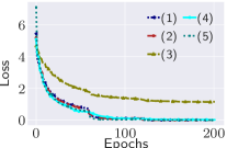
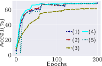
(1)	SGD	0.012	99.91	1.405	68.57	4262
(2)	ASSM	0.010	99.95	1.390	68.12	3545
(3)	PASSM	1.146	69.88	1.414	61.40	1773
(4)	PASSM$+$	0.030	99.63	1.224	68.59	2668
(5)	SGD (BS=1024)	0.006	99.97	1.533	68.15	3179

(a) Performance Summary.

(b) Train Loss.

(c) Top1 Val Accuracy.

Figure 2: First, we take the case of a relatively small architecture, Shufflenet [34] with 1012108 parameters, training over CIFAR100 on the setting S1. The memory footprint for baseline SGD with BS=128 is $\sim$2.1 GB. The asynchronous methods use BS=128 and train with 4 processes. The large-batch training gets LR warm-up. The initial LR, weight-decay, momentum are identical across the methods. PASSM$+$ provides 1.2x speed-up compared to the large-batch method and 1.6x compared to the baseline with a superior validation accuracy.

	Algo	Train Loss	Train Acc@1	Test Loss	Test Acc@1	Time (Sec)
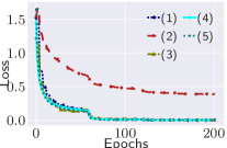
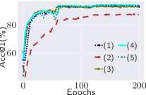
(1)	ASSM	0.001	99.99	0.287	93.45	17570
(2)	PASSM	0.383	92.75	0.391	87.41	9659
(3)	PASSM$+$	0.002	99.99	0.324	94.07	13047
(4)	SGD	0.002	99.99	0.273	94.36	16199
(5)	SGD (BS=512)	0.001	99.99	0.297	93.93	15314

(a) Performance Summary.

(b) Train Loss.

(c) Top1 Val Accuracy.

Figure 3: Now, we consider WideResnet16x8 [34] with 11012036 parameters training over CIFAR10 on the setting S1. The initial LR, weight-decay, momentum are identical across the methods. The memory footprint for SGD with BS=64 is $\sim$2 GB. Here we compute subgradients with BS=64 and update the model at BS=128 for the baseline SGD and the asynchronous methods, which spawn 4 concurrent processes for training. The large-batch SGD computes subgradients with BS=256, and updates the model with BS=512, and is given LR warm-up. Notice that as the model size grows, we face memory constraints and higher training time, which clearly needs scaling. In this set of experiments, PASSM$+$ achieves 1.25x speed-up in comparison to baseline and 1.17x in comparison to a large-batch method, with a generalization performance at par.

Algo	Dataset	Train Loss	Train Acc@1	Test Loss	Test Acc@1	Time (Sec)
(1) SGD	C100	0.005	99.97	1.355	74.31	4478
(2) SGD	C10	0.002	99.99	0.290	93.35	3751
(3) PASSM$+$	C100	0.004	100.00	1.402	74.67	3827
(4) PASSM$+$	C10	0.002	99.99	0.302	93.33	3307

(a) Performance Summary.

(b) Train Loss.

(c) Top1 Val Accuracy.

Figure 4: Finally we consider an architecture with even bigger memory requirement, Densenet121 [17] with 7048548 parameters, training over CIFAR10/100 (C10/100). Its memory footprint of $\sim$6.2 GB with BS=128 for SGD makes it practical to train on the distributed setting S2. Here SGD is decentralized over 10 GPUs and is implemented by a state-of-the-art (SOTA) framework DistributedDataParallel of Pytorch. PASSM$+$ spawns 3 concurrent PSs. Here SGD is a large-batch implementation, which computes subgradients at BS=128 and updates the model at BS=1280 on aggregation. On the other hand, the slaves of each PS compute subgradient at BS=128 and the PSs themselves compute subgradient at BS=32 in order for load-balancing at the shared GPU. We do LR warm-up for both the methods. Because the updates by PSs and SGD have different BSs, we use different LR for them, essentially in the ratio of their BSs: $\frac{416}{1280}$. The weight-decay and momentum are identical across the methods. Compared to the SOTA implementation, PASSM$+$ provides speed-up of 1.17x for CIFAR100 and 1.13x for CIFAR10 with matching validation accuracy. We can explain the speed-up in terms of (a) reduced flops during backpropagation, (b) reduced communication cost for partitioned subgradients across GPUs, and (c) potentially reduced synchronization cost in a distributed setting.

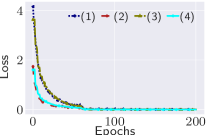
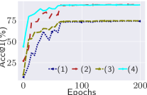
During the course of an end-to-end training, a standard diminishing learning rate (LR) scheme is the following: the LR is dampened by a constant factor $\gamma$ when a fixed portion of the sample-processing budget is consumed. A common practice is to dampen LR when 50% and 75% samples are processed. Some practitioners also prefer dampening LR when 30%, 60% and 80% samples are processed [14].

Now, an immediate clue to improve the optimization by PASSM would be to spend some floating point operations saved by partitioned subgradient computation. We observed that during the initial phase of training, doing full subgradient updates helps. However, on further exploration we noticed that even if we perform full subgradient updates during the first 50% number of epochs, it was insufficient for PASSM to recover the same level of train and validation accuracy. Furthermore, we noticed that doing the full subgradient updates during a small number of epochs around LR dampening steps would improve the convergence results.

Based on these observations, we developed the following heuristic. We perform roughly 25% ASSM iterations initially. After that we switch to PASSM iterations. Further down the course of optimization, we throw in roughly 10% ASSM iterations around the LR dampening phase, thus in total performing roughly 50% ASSM and 50% PASSM iterations. On top of this, we marginally dampen the LR by a factor of $(1-1/c)$, where $c>1$ is the number of concurrent processes, when switching from ASSM to PASSM. Our experiments show that this heuristic was good enough to almost always recover the optimization quality that full subgradient computation methods would achieve.

Experimental Observations, Discussions and Summary.

We present detailed observations and discussions thereof for a number of well-known CNN architectures for image classification in Figures 2, 3, and 4. Each of the experimental runs is seeded, however, there is always a system-dependent randomization in asynchronous updates due to multiprocessing. Therefore, we take the average of three runs.

Hyperparameter tuning for optimization of neural networks is a challenging task for practitioners [31]. Many existing work particularly suggest tuning other hyperparameters such as momentum [32, 33]. Yet others tune the learning rate adapted to the performance on dev set [7]. In comparison to these methods, our heuristic is simple enough, yet we believe that on further tuning the hyperparameters PASSM$+$ would be an extremely efficient method that would save on computation with a quality solution for neural network training. In the experiments, we followed the well-accepted strategies with respect to the system components, such as number of CPU threads to load data, to run the baseline; it is especially encouraging to see that PASSM$+$ outperforms SOTA on this count.

5 Conclusion

In this paper we analyzed the convergence theory of asynchronous parallel stochastic subgradient descent. Under a realistic probabilistic model of asynchronous parallel architecture applied to the stochastic subgradient method with momentum, we showed asymptotic convergence to a stationary point of general nonconvex nonsmooth objectives.

We presented numerical results that indicate that the theory suggests an efficient implementation strategy for this class of optimization methods to train deep neural networks.

Appendix A The Probabilistic Computation Model

A.1 Motivation

Classical convergence analysis for parallel asynchronous optimization using shared memory has been based on a simplistic model of asynchronous computation. In particular, it is assumed that every block of the parameter vector has an equal probability of being updated at every iteration. Moreover, the delay between the the age of each block at each core and the shared memory is fixed. As a consequence, each core reads and updates each block in a symmetric fashion.

The simplistic model of asynchronous computation in [35, 21] is also not consistent with standard practice in real processing architectures. For example, in the common Non-Uniform Memory Access (NUMA) architecture, experiments have shown that it can be more effective for each core to update only a subset of blocks. As such, the block that is updated at each iteration depends on the previous iterates and the last core to update. This induces a probabilistic dependence between delays and the block to be updated.

To account for these realistic features of asynchronous computation, we consider the model given in [5] and apply it to the stochastic approximation scheme. In this work, an algorithm based on successive convex approximation and coordinate-wise updates was also proposed and analysed.

A.2 Algorithm from the “Global" Perspective

We first reformulate Algorithm 1 from the perspective of a global counter, indicating sequential updates of any variable block by any core. In iteration $k$, the updated iterate $x_{i^{k}}^{k+1}$ depends on a random vector $\zeta^{k}\overset{\triangle}{=}(i^{k},d^{k},\xi^{k})$, where $i^{k}$ is the variable block to be updated, while $d^{k}$ and $\xi^{k}$ are the vector of delays for the variables and the set of mini-batches, respectively, for the core performing the update. With this notation, Algorithm 1 in the main text can be rewritten from the global perspective as given in Algorithm 2 here.

Algorithm 2 Asynchronous Stochastic Subgradient Method with a Global Counter

1:  Input: $x_{0}$.

2:  for $k=1,2,\ldots$ do

3:     Sample $\zeta^{k}=(i^{k},d^{k},\xi^{k})$.

4:     Update $u_{i^{k}}\leftarrow mu_{i^{k}}+g_{i^{k}}(x^{k},\xi^{k})$

5:     Update $x^{k+1}_{i^{k}}\leftarrow x^{k}_{i^{k}}-(1-m)\gamma^{\nu(k)}u_{i^{k}}$

6:     $k\leftarrow k+1$

7:  end for

In order to obtain global convergence, we require a diminishing step size. However, as synchronization is not feasible, each core does not necessarily have access to a global counter to inform the step size decrease. Instead, each core has its own local step size $\gamma^{\nu(c^{k},k)}$, where $c^{k}$ is the core in the $k$-th global iteration. We also define the random variable $Z^{k}$ as the element of $\{1,\ldots,\overline{c}\}$ that is active in global iteration $k$. The random variable $\nu(c^{k},k)\overset{\triangle}{=}\sum_{j=0}^{k}I(Z^{j}=c^{k})$ denotes the number of updates performed by core $c^{k}$ before the $k$-th iteration.

In practice, it has been observed that it is more efficient to partition variable blocks over the cores, rather than allowing every processor to update any variable block [23]. Using this approach, $c^{k}$ is uniquely defined by $i^{k}$, the block variable index updated in iteration $k$.

A.3 Continuous-Time Reformulation of the Probabilistic Model

Recall the update mechanism for the Algorithm

$$x_{i^{k+1}}^{k+1}=x_{i^{k}}^{k+1}+(1-m)\gamma^{k,i}\sum_{j=1}^{k}m^{k-j}Y_{j,i},$$ (8)

where $Y_{j,i}$ is based on an estimate of the partial subgradient with respect to block variables indexed by $i$ at local iteration $j$.

In the context of Algorithm 1, the step size is defined to be the subsequence $\{\gamma^{k,i}\}=\{\gamma^{\nu(c(i),l)}:i=i^{l}\}$ where $l$ is the iteration index for the core corresponding to block $i$. That is, the step size sequence forms the subsequence of $\gamma^{k}$ for which $i^{k}=i$ is the block of variables being modified.

The term $Y_{k,i}$ corresponds to $g(x_{k},\xi)$ and satisfies,

$$Y_{k,i}=g_{i}((x_{k-[d^{k}_{i}]_{1},1},...,x_{k-[d^{k}_{i}]_{j},j},...,x_{k-[d^{k}_{i}]_{n},n}))+\beta_{k,i}+\delta M_{k,i},$$

where $g_{i}(x)$ denotes a selection of an element of the subgradient, with respect to block $i$, of $f(x)$. The quantity $\delta M_{k,i}$ is a martingale difference sequence, satisfying $\delta M_{k,i}=M_{k+1,i}-M_{k,i}$ for a martingale $M_{k}$, a sequence of random variables which satisfies $\mathbb{E}[M_{k,i}]<\infty$ and $\mathbb{E}[M_{k+1,i}|M_{j,i},j\leq k]=M_{k,i}$ with probability $1$ for all $k$. It then holds that $\mathbb{E}[|M_{k,i}|^{2}]<\infty$ and $\mathbb{E}[M_{k+1,i}-M_{k,i}][M_{j+1,i}-M_{j,i}]^{\prime}=0$. As a consequence, $\mathbb{E}_{k,i}[\delta M_{k,i}]=0$.

The assumption that $\delta M_{k,i}$ forms a martingale difference sequence is a common condition, which was introduced by the original Robbins-Monro method [29]. In particular, the martingale difference sequence assumption holds when the stochastic gradient estimate is obtained from a subset $\xi\subseteq\{1,...,M\}$ of mini-batches sampled uniformly from the set of size $|\xi|$ of subsets of $\{1,...,M\}$, independently at each iteration. This results in independent noise at each iteration being applied to the stochastic subgradient term. From these mini-batches $\xi$, a subgradient is taken for each $j\in\xi$ and averaged; i.e.,

$$g(x,\xi)=\frac{1}{|\xi|}\sum_{j\in\xi}g^{j}(x)$$ (9)

where $g^{j}(x)\in\partial f_{j}(x)$.

Appendix B Relationship to the Probabilistic Model of Asynchronous Computation

We now relate the assumptions we have presented so far to this model for inconsistent read given in [5].

To this end, define $\underline{\zeta}^{0:t}\triangleq(\underline{\zeta}^{0},\underline{\zeta}^{1},...,\underline{\zeta}^{t})$ to be a sequence of the blocks and minibatches used, as well as the iterate delays. To measure this process, define the sample space $\Omega$ of all sequences $\{\underline{\zeta}^{k}\}_{k}$. To define a $\sigma$-algebra on $\Omega$, for every $k\geq 0$ and every $\underline{\zeta}^{0:k}$, consider the cylinder

$$C^{k}(\underline{\zeta}^{0:k})\overset{\triangle}{=}\{\omega\in\Omega:\omega_{0:k}=\underline{\zeta}^{0:k}\},$$ (10)

where $\omega_{0:k}$ is the first $k+1$ elements of $\omega$. Denote $\mathcal{C}^{k}$ as the set of $C^{k}(\underline{\zeta}^{0:k})$ for all possible values of $\underline{\zeta}^{0:k}$. Let $\sigma(\mathcal{C}^{k})$ be the cylinder $\sigma$-algebra generated by $\mathcal{C}^{k}$, and define for all $k$,

$$\mathcal{F}_{k}=\sigma(\mathcal{C}^{k}),~{}~{}~{}\mathcal{F}\overset{\triangle}{=}\sigma(\cup_{t=0}^{\infty}\mathcal{C}^{t}).$$ (11)

With a probability measure $\mathbb{P}(C^{k}(\underline{\zeta}^{0:k}))$ satisfying standard assumptions (detailed in [5]), induces a probability measure $P$ such that $(\Omega,\mathcal{F},P)$ forms a probability space. This provides a means of formalizing the discrete-time stochastic process $\zeta$ where $\underline{\zeta}$ is a sample path of the process.

The conditional probabilities $\mathbb{P}(\zeta^{k+1}=\omega^{k+1}|\zeta^{0:k}=\omega^{0:k})$ are then defined by

$$p(\zeta^{k+1}|\zeta^{0:k})=\mathbb{P}(\zeta^{k+1}=\omega^{k+1}|\zeta^{0:k}=\omega^{0:k})=\frac{\mathbb{P}(C^{k+1}(\zeta^{0:k+1}))}{\mathbb{P}(C^{k}(\zeta^{0:k}))}$$ (12)

In [5], the following assumptions were introduced for the probabilities of block selection and the delays.

Assumption B.1.

The process $\{\zeta^{k}\}_{k}$ satisfies,

1. There exists a $\delta$ such that $d^{k}_{j}\leq\delta$ for all $j$ and $k$. Thus each $d^{k}_{j}\in\mathcal{D}\triangleq\{0,...,\delta\}^{n}$.

2. For all $i$ and $\zeta^{0:k-1}$ such that $p_{\zeta^{0:k-1}}(\zeta^{0:k-1})>0$, it holds that,

   $$\sum_{d\in\mathcal{D}}p((i,d,\xi)|\zeta^{0:k-1})\geq p_{min}$$

   for some $p_{min}>0$.

3. It holds that,

   $$\mathbb{P}\left(\left\{\zeta\in\Omega:\liminf_{k\to\infty}p(\zeta|\zeta^{0:k-1})>0\right\}\right)=1$$

The first condition is an irreducibility condition that there is a positive probability for any block or minibatch to be chosen, given any state of previous realizations of $\{\zeta^{k}\}$. The second assumption indicates that the set of events in $\Omega$ that asymptotically go to zero in conditional probability are of measure zero.

We note that $\liminf_{k\to\infty}\frac{\gamma^{\nu(c^{k},k)}}{k}=0$ in probability is implied by

$$\sum_{i\in c^{k},d\in\mathcal{D},\xi\subseteq\{1,...,M\}}Pr((i,d,\xi)|\zeta^{0:k-1}))\to 0$$

for some subsequence, which is antithetical to Assumption B.1(i). Thus, the step-sizes $\gamma^{\nu(c^{k},k)}$ satisfy

$$\liminf_{k\to\infty}\frac{\gamma^{\nu(c^{k},k)}}{k}>0,$$ (13)

where the limit of the sequence is taken in probability. This is also an assumption for the analysis of stochastic asynchronous parallel algorithms in the simplified model developed in [3].

Appendix C Proofs of the Theoretical Results

C.1 Preliminaries

Lemma C.1.

It holds that $\{Y_{k,i},Y^{\sigma}_{k,i};k,i\}$ is uniformly integrable. Thus, so is

$$\left\{\sum_{j=1}^{k}m^{k-j}Y_{j,i},\sum_{j=1}^{k}m^{k-j}Y^{\sigma}_{j,i};k,i\right\}$$

Proof.

Uniform integrability of $\{Y_{k,i},Y^{\sigma}_{k,i};k,i\}$ follows from Assumption 3.2, part 3. The uniform integrability of $\left\{\sum_{j=1}^{k}m^{k-j}Y_{j,i},\sum_{j=1}^{k}m^{k-j}Y^{\sigma}_{j,i};k,i\right\}$ follows from $0<m<1$ and the fact that a geometric sum of a uniformly integrable sequence is uniformly integrable. ∎

Lemma C.2.

It holds that, for any $K>0$, and all $l$,

$$\sup_{k<K}\sum_{j=k-[d^{k}_{i}]_{l}}^{k}\gamma^{\sigma}_{j,i}\to 0$$

in probability as $\sigma\to\infty$.

Proof.

As $\sigma\to\infty$, by the definition of $\gamma^{\sigma}_{k,i}$, $\gamma^{\sigma}_{k,i}\to 0$ and since by Assumption 3.1 $\max d^{k}_{i}\leq\delta$, for all $k<K$, $\sum_{j=k-[d^{k}_{i}]_{l}}^{k}\gamma^{\sigma}_{j,i}\leq\delta\gamma^{\sigma}_{k-\delta,i}\to 0$. ∎

Our main convergence result establishes weak convergence of trajectories to an invariant set. Weak convergence is defined in terms of the Skorohod topology, a technical topology weaker than the topology of uniform convergence on bounded intervals, defined in [8]. Convergence of a function $f_{n}(\cdot)$ to $f(\cdot)$ in the Skorohod topology is equivalent to uniform convergence on each bounded time interval. We denote by $D^{j}(-\infty,\infty)$ the $j$-fold product space of real-valued functions on the interval $(-\infty,\infty)$ that are right continuous with left-hand limits, with the Skorohod topology forming a complete and separable metric space.

We present a result indicating sufficient conditions for tightness of a set of paths in $D^{j}(-\infty,\infty)$.

Theorem C.1.

[19, Theorem 7.3.3] Consider a sequence of processes $\{A_{k}(\cdot)\}$ with paths in $D^{j}(-\infty,\infty)$ such that for all $\delta>0$ and each $t$ in a dense set of $(-\infty,\infty)^{j}$ there is a compact set $K_{\delta,t}$ such that,

$$\inf_{n}\mathbb{P}\left[A_{n}(t)|\in K_{\delta,t}\right]\geq 1-\delta,$$

and for any $T>0$,

$$\lim_{\delta\to 0}\limsup_{n}\sup_{|\tau|\leq T}\sup_{s\leq\delta}\mathbb{E}\left[\min\left[|A_{n}(\tau+s)-A_{n}(\tau)|,1\right]\right]=0$$

then $\{A_{n}(\cdot)\}$ is tight in $D^{j}(-\infty,\infty)$.

If a sequence is tight then every weak sense limit process is also a continuous time process. We say that $A_{k}(t)$ converges weakly to $A$ if,

$$\mathbb{E}\left[F(A_{k}(t))\right]\to\mathbb{E}\left[F(A(t))\right]$$

for any bounded and continuous real-valued function $F(\cdot)$ on $\mathbb{R}^{j}$.

Finally, an invariant set for a differential inclusion (DI) is defined as follows.

Definition C.1.

A set $\Lambda\subset\mathbb{R}^{n}$ is an invariant set for a DI $\dot{x}\in g(x)$ if for all $x_{0}\in\Lambda$, there is a solution $x(t)$, $-\infty<t<\infty$ that lies entirely in $\Lambda$ and satisfies $x(0)=x_{0}$.

C.2 Proof of Theorem 3.1

Remark C.1.

The proof of Theorem 3.1 largely follows an analogous result in Chapter 12 of [19], which considers a particular model of asynchronous stochastic approximation. As we focus on a different model for asynchronous updates, some of the details of the proof are now different. We have also modified the proof to account for momentum.

By [11, Theorem 8.6, Chapter 3], a sufficient condition for tightness of a sequence $\{A_{n}(\cdot)\}$ is that for each $\delta>0$ and each $t$ in a dense set in $(-\infty,\infty)$, there is a compact set $K_{\delta,t}$ such that $\inf_{n}\mathbb{P}[A_{n}(t)\in K_{\delta,t}]\geq 1-\delta$ and for each positive $T$,

$$\lim_{\delta\to 0}\limsup_{n}\sup_{|\tau|\leq T,\,s\leq\delta}\mathbb{E}\left[|A_{n}(\tau+s)-A_{n}(\tau)|\right]=0.$$

Now since $Y_{k,i}$ is uniformly bounded, and $Y^{\sigma}_{k,i}(\cdot)$ is its interpolation with jumps only at $t$ being equal to some $T_{k,i}$, it holds that for all $i$,

$$\lim_{\delta\to 0}\limsup_{\sigma}\mathbb{P}\left[\sup_{t\leq T,\,s\leq\delta}|Y^{\sigma}_{k,i}(t+s)-Y^{\sigma}_{k,i}(t)|\geq\eta\right]=0$$

and so by the definition of the algorithm,

$$\lim_{\delta\to 0}\limsup_{\sigma}\mathbb{P}\left[\sup_{t\leq T,\,s\leq\delta}|x^{\sigma}_{k,i}(t+s)-x^{\sigma}_{k,i}(t)|\geq\eta\right]=0$$

which implies,

$$\lim_{\delta\to 0}\limsup_{\sigma}\mathbb{E}\left[\sup_{t\leq T,\,s\leq\delta}|x^{\sigma}_{k,i}(t+s)-x^{\sigma}_{k,i}(t)|\right]=0$$

and the same argument implies tightness for $\{\tau^{\sigma}_{i}(\cdot),N^{\sigma}_{i}(\cdot)\}$ by the uniform boundedness of $\{\delta\tau^{\sigma}_{i,k}\}$ and bounded, decreasing $\gamma^{\sigma}_{k,i}$ and positive $u^{\sigma}_{k,i}(x,\psi^{\sigma}_{k+1,i})$, along with Assumption 2.4. Lipschitz continuity follows from the properties of the interpolation functions. Specifically, the Lipschitz constant of $x^{\sigma}_{i}(\cdot)$ is $B_{g}$.

All of these together imply tightness of $\hat{x}^{\sigma}_{i}(\cdot)$ as well. Thus,

$$\{x^{\sigma}_{i}(\cdot),\tau^{\sigma}_{i}(\cdot),\hat{x}^{\sigma}_{i}(\cdot),N^{\sigma}_{i}(\cdot);\sigma\}$$

is tight in $D^{4n}[0,\infty)$. This implies the Lipschitz continuity of the subsequence limits with probability one, which exist in the weak sense by Prohorov’s Theorem, Theorems 6.1 and 6.2 [2].

As $\sigma\to\infty$ we denote the limit of the weakly convergent subsequence by,

$$(x_{i}(\cdot),\tau_{i}(\cdot),\hat{x}_{i}(\cdot),N_{i}(\cdot))$$

Note that,

$$\begin{array}[]{l}x_{i}(t)=\hat{x}_{i}(\tau_{i}(t)),\\ \hat{x}_{i}(t)=x_{i}(N_{i}(t)),\\ N_{i}(\tau_{i}(t))=t.\end{array}$$

For more details, see the proof of  [19, Theorem 8.2.1].

Let,

$$\begin{array}[]{l}M^{\sigma}_{i}(t)=\sum_{k=0}^{k=p(\sigma)}(1-m)\delta\tau_{k,i}\left(\sum_{j=0}^{k}m^{j}\delta M^{\sigma}_{k-j,i}\right)\\ \tilde{G}_{i}^{\sigma}(t)=\sum_{k=0}^{k=p(\sigma)}\delta\tau_{k,i}\left[(1-m)\sum_{j=0}^{k}m^{j}g_{i}((x^{\sigma}_{{k-j}-[d^{k-j}_{i}]_{1},1}(t),...,\right.\\ \qquad\qquad\left.x^{\sigma}_{{k-j}-[d^{k-j}_{i}]_{j},j}(t),...,x_{{k-j}-[d^{k-j}_{i}]_{N},N}))(t)-g_{i}(\hat{x}^{\sigma}_{i}(t))\right]\\ \bar{G}_{i}^{\sigma}(t)=\sum_{k=0}^{k=p(\sigma)}\delta\tau_{k,i}g_{i}(\hat{x}^{\sigma}(t))\\ B_{i}^{\sigma}(t)=\sum_{k=0}^{\rho(\sigma)}(1-m)\delta\tau_{k,i}\left(\sum_{j=0}^{k}m^{j}\beta_{k-j,i}^{\sigma}\right)\\ W^{\sigma}_{i}(t)=\hat{x}^{\sigma}_{i}(\tau^{\sigma}_{i}(t))-x^{\sigma}_{i,0}-\bar{G}_{i}^{\sigma}(t)=\tilde{G}_{i}^{\sigma}(t)+M^{\sigma}_{i}(t)\end{array}$$

Now for any bounded continuous and real-valued function $h(\cdot)$, an arbitrary integer $p$, and $t$ and $\tau$, and $s_{j}\geq t$ real, we have

$$\begin{array}[]{l}\mathbb{E}\left[h(\tau^{\sigma}_{i}(s_{j}),\hat{x}^{\sigma}(\tau^{\sigma}_{i}(s_{j}))\left(W^{\sigma}_{i}(t+\tau)-W^{\sigma}_{i}(t)\right)\right]\\ \qquad-\mathbb{E}\left[h(\tau^{\sigma}_{i}(s_{j}),\hat{x}^{\sigma}(\tau^{\sigma}_{i}(s_{j}))\left(\tilde{G}^{\sigma}_{i}(t+\tau)-\tilde{G}^{\sigma}_{i}(t)\right)\right]\\ \qquad-\mathbb{E}\left[h(\tau^{\sigma}_{i}(s_{j}),\hat{x}^{\sigma}(\tau^{\sigma}_{i}(s_{j}))\left(M^{\sigma}_{i}(t+\tau)-M^{\sigma}_{i}(t)\right)\right]\\ \qquad-\mathbb{E}[h(\tau_{i}^{\sigma}(s_{j}),\hat{x}^{\sigma}(\tau_{i}^{\sigma}(s_{j})))(B_{i}^{\sigma}(t+\tau)-B_{i}^{\sigma}(t))]=0.\end{array}$$

Now the term involving $M^{\sigma}$ equals zero from the Martingale property. The term involving $B^{\sigma}$ is zero due to Assumption 2.5.

We now claim that the term involving $\tilde{G}^{\sigma}_{i}$ goes to zero as well. Since $x^{\sigma}_{k,i}\to x^{\sigma}_{i}$ it holds that, by Lemma C.2, $(x^{\sigma}_{k-[d^{k}_{i}]_{1},1}(t),...,x^{\sigma}_{k-[d^{k}_{i}]_{j},j}(t),...,x^{\sigma}_{k-[d^{k}_{i}]_{N},N})\to\hat{x}^{\sigma}(t)$ as well. By the upper semicontinuity of the subgradient, it holds that there exists a $g_{i}(\hat{x}^{\sigma}_{i}(t))\in\partial_{i}f(\hat{x}^{\sigma}_{i}(t))$ such that

$$g_{i}((x^{\sigma}_{k-[d^{k}_{i}]_{1},1}(t),...,x^{\sigma}_{k-[d^{k}_{i}]_{j},j}(t),...,x_{k-[d^{k}_{i}]_{N},N}))(t)\to g_{i}(\hat{x}^{\sigma}_{k}(t))$$

as $\sigma\to\infty$. Thus each term in the sum converges to $g_{i}(\hat{x}^{\sigma}_{k-j}(t))$. Now, given $j$, as $k\to\infty$, the boundedness assumptions and stepsize rules imply that $g_{i}(\hat{x}^{\sigma}_{k-j}(t))\to g_{i}(\hat{x}^{\sigma}_{k}(t))$. On the other hand as $k\to\infty$ and $j\to\infty$, $m^{j}g_{i}(\hat{x}^{\sigma}_{k-j}(t))\to 0$. Thus

$$\sum_{j=0}^{k}m^{j}g_{i}(\hat{x}^{\sigma}_{k-j}(t))\to\frac{1-m^{k}}{1-m}g_{i}(\hat{x}^{\sigma}_{k}(t))\to\frac{1}{1-m}g_{i}(\hat{x}^{\sigma}_{k}(t))$$

and the claim has been shown.

So the weak sense limit of $\lim_{\sigma\to\infty}W^{\sigma}_{i}(\cdot)=W_{i}(\cdot)$ satisfies

$$\mathbb{E}\left[h(\tau_{i}(s_{j}),\hat{x}(\tau_{i}(s_{j}))\left(W_{i}(t+\tau)-W_{i}(t)\right)\right]$$

and by  [19, Theorem 7.4.1] is a martingale and is furthermore a constant with probability one by the Lipschitz continuity of $x$ by  [19, Theorem 4.1.1]. Thus,

$$W(t)=\hat{x}(t)-\hat{x}(0)-\int_{0}^{t}g(\hat{x}(s))ds=0,$$

where $g(\hat{x}(s))\in\partial f(\hat{x}(s))$, and the conclusion holds.

C.3 Convergence with Probability One

Theorem C.2.

There exists a functional $\overline{S}(x,T,\phi)$ defined for $x\in\mathbb{R}^{n},T>0,\phi(\cdot)\in C[0,T]$ satisfying:

1. There exists $\overline{b}(x)$ such that $\overline{S}(x,T,\phi)=0$ if and only if $\dot{\phi}\in\overline{b}(\phi)$ almost surely, $\phi(0)=x$.

2. $\overline{S}(x,T,\phi)\geq 0$.

3. Given compact $F\subset\mathbb{R}^{n}$, $T>0$, and $s\in[0,\infty)$, the set $\{\phi:\phi(0)\in F,\overline{S}(\phi(0),T,\phi)\leq s\}$ is compact.

4. Given compact $F\subset\mathbb{R}^{n}$, $T>0$, $h>0$ and $s\in[0,\infty)$,

   $$\limsup_{\sigma\rightarrow\infty}\gamma_{p_{i}(\sigma),i}\log P(\hat{x}_{i}^{\sigma}(\cdot))\not\in N_{h}(\Phi(\hat{x}_{i}^{\sigma}(0),T,s))|\mathcal{F}_{p_{i}(\sigma),i})\leq-s$$ (14)

   uniformly in $\hat{x}_{i}^{\sigma}(0)\in F$

Proof.

Since the noise is bounded by Assumption 2.2, [9, Theorem 4.1] and [9, Theorem 5.3] hold without any changes. ∎

The next step is to modify [9, Theorem 3.1]. The main change is to replace [9, Assumption 2.2] with the existence of a solution to the DI in Theorem 3.1 and an invariant set. The impact of this change on the proof is to replace any mention of the trajectory lying in a ball around a limit point with a ball around the invariant set. The result of this modification is then that for each $i$ under Theorem 3.1 as $\sigma\rightarrow\infty$, $\hat{x}_{i}^{\sigma}(\cdot)$ converges to an invariant set of the DI in Theorem 3.1 with probability one.

C.4 Properties of the Limit Point

Finally, we wish to characterize the properties of this invariant set. Training neural networks induces optimization problems with an objective of the form $f(x)=\ell(y_{j},a_{L})$, where $\ell(\cdot)$ is a standard loss function, and $a_{L}$—depending on the activation functions from each layer $a_{i},~{}i=1,\ldots,L$—is obtained recursively via $a_{i}=\rho_{i}(V_{i}(x)a_{i-1}),~{}i=1,\ldots,L$. These activation functions are typically defined to be piece-wise continuous functions constructed from $\log x$, $e^{x}$, $\max\{0,x\}$ or $\log(1+e^{x})$. In this case, it follows from [6, Corollary 5.11] that the set of invariants $\{x^{*}\}$ satisfy $0\in\partial f(x^{*})$. Moreover, for any iterative algorithm generating $\{x^{k}\}$ such that $x^{k}\rightarrow x^{*}$, the values $f(x^{k})$ converge to $f(x^{*})$.

Theorem 3.1 and Theorem 3.2 provide guarantees on convergence to block-wise stationary points; i.e., for each $i$, $0\in\partial_{i}f(x)$. As such, every stationary point is also block-wise stationary, which implies that $0\in\partial f(x)$ implies $0\in\partial_{i}f(x)$ for all $i$.

To ensure convergence to a stationary point, a variant of Algorithm 2 can be used, in particular ASSM, where every core updates the entire vector (no block partitioning), but locks the shared memory whenever the core either reads or writes. The analysis in this Section also applies to this case. In particular, $i^{k}=\{1,...,n\}$ for all $k$ and every limit of $x^{\sigma}(t)$ as either $\sigma\to\infty$ or $t\to\infty$ is a critical point of $f(x)$ and, with probability one, asymptotically the algorithm converges to a critical point of $f(x)$ (i.e., $x$ such that $0\in\partial f(x)$).

Appendix D Experiment Description and Additional Numerical Results

System Detail.

Referring to the settings S1 and S2 as in Section 4 of the main submission, the following detail apply:

• : A workstation with a single socket Intel(R) Xeon(R) CPU E5-1650 v4 running @ 3.60 GHz with 6 physical cores amounting to 12 logical cores with hyperthreading. A single Nvidia GeForce RTX 2080 Ti GPU is connected to the motherboard via a PCIe GEN 1@16x interface which allows data transfer speed up to 4 GB/s. We use 4 concurrent processes with 3 threads each to fetch data from the main-memory to the GPU in SGD and for asynchronous methods each process uses 3 threads and no multiprocessing for data transfer. Clearly, the CPU resources are optimally allocated, which we check before starting the experiments. The system has 64 GB main memory sufficient to buffer the entire dataset for CIFAR10/CIFAR100/SVHN. It runs on Ubuntu 18.04.4, Linux 4.15.0-101-generic operating system.

• : A NUMA workstation with two sockets containing Intel(R) Xeon(R) CPU E5-2650 v4 running @ 2.20 GHz with 12 physical cores amounting to 24 logical cores apiece with hyperthreading. 10 Nvidia GeForce RTX 1080 Ti GPUs are connected to the same motherboard via PCIe GEN 3@16x interfaces which can enable data transfer between the main-memory and GPU up to 16 GB/s. We use 2 concurrent processes with 2 threads each to fetch data from the main-memory to the GPU by decentralized SGD processes running on each of the GPUs; for asynchronous methods each parameter server process uses 2 threads and no multiprocessing for data transfer, whereas its slaves utilize 2 concurrent processes with 2 threads each for the same. The system has 256 GB main memory. It runs on Debian GNU/Linux 9.12 operating system.

Restricted Backpropagation.

Consider the shared-memory system with $c$ concurrent processes and a model of size $w$ with requirement of $F$ flops for a backpropagation over its computation graph. As described before, we distribute roughly $w/c$ parameters as in a partition to each of the processes. Now, the process assigned with the partition that includes the input layer, has to pay the cost of full backpropagation i.e. $F$. Traversing from the partition that includes the input layer to the one that includes the output layer, the saving by the processes would be $0,\frac{F}{c},\frac{2F}{c},\ldots,\frac{(c-1)F}{c}$ flops per backpropagation. Summing it up, we have total savings of $F\frac{(c-1)}{2}$ flops in $c$ concurrent backpropagation steps by $c$ processes. It is imperative that on average PASSM saves roughly $\frac{3F}{8}$ flops per backpropagation carried out by 4 concurrent processes in our experiments.

Additional Experiment.

Now, we present an example in which even PASSM itself recovers the classification accuracy achieved by the baseline, see Figure 5 and the description thereof.

	Algo	Train Loss	Train Acc@1	Test Loss	Test Acc@1	Time (Sec)
(1)	ASSM	0.001	100.00	0.234	93.95	1332
(2)	PASSM	0.029	99.47	0.221	93.75	726
(3)	SGD	0.001	100.00	0.267	93.30	964
(4)	SGD (BS:1024)	0.001	100.00	0.246	93.83	1366

(a) Performance Summary.

(b) Train Loss.

(c) Top1 Val Accuracy.

Figure 5: We consider Resnet34 [16] with 21289802 parameters, training over SVHN [26] dataset. This training experiment has a relatively small memory footprint of $\sim$1.3 GB with BS=256 for SGD. We train it on the setting S1, see Section 4 in the main submission. The asynchronous methods train with 4 concurrent processes and compute subgradients at BS=256. The baseline minibatch SGD too computes subgradients at BS=256, whereas the large minibatch method computes subgradients at BS=1024. We give LR warm-up to the large minibatch method. The initial LR, weight-decay and momentum are identical across the methods. Each of the training instances are run for 90 epochs. The LR is dampened by $\frac{1}{10}$ at 30, 60 and 80 epochs and no other variation. In this case, PASSM itself was sufficient to recover the generalization accuracy at par with the baseline and outperforming the large minibatch training. Compared to the large minibatch method, PASSM provides speed-up of 1.33x, whereas compared to the baseline its speed-up is 1.88x. This example shows that in those cases, where we have a relatively deeper model and relatively smaller image sizes – SVHN dataset contains 73257 training images and 26032 test images of small cropped digits of size 32x32, PASSM itself is sufficient to train the model with classification accuracy at par with the baseline without applying the heuristic approach.

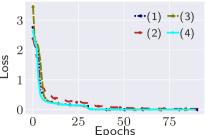
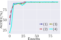
Hyperparameters’ Details.

We had already mentioned the minibatch-size and the number of processes or parameter-servers used in the experiments before. The remaining hyperparameters of the experiments are provided in Table 1.

Experiment	Epochs	Init. LR	$\gamma$	Dampening at	Weight decay	PASSM$+$ switch at
S1: ResNet20/CIFAR10/100	300	0.1	0.1	150, 225	0.0005	75, 135, 165, 210, 225
S1: Shufflenet/CIFAR100	200	0.1	0.2	60, 120, 160	0.0001	30, 50, 70, 110, 130, 150, 170
S1: WideResNet16x8/CIFAR10	200	0.1	0.2	60, 120, 160	0.0001	30, 50, 70, 110, 130, 150, 170
S2: Densenet121/CIFAR100	200	0.1	0.2	60, 120, 160	0.0001	30, 50, 70, 110, 130, 150, 170
S1: ResNet34/SVHN	90	0.1	0.1	30, 60, 80	0.0005	–

Table 1: Hyperparameters used in the experiments.

In each of the experiments, we have a constant momentum of 0.9. PASSM$+$ starts with ASSM iterations i.e. computes and applies full subgradient updates, thereafter switches to PASSM and back to ASSM at the epoch counts as mentioned in Table 1. In large minibatch training, the warm-up procedure starts the learning rate as the initial learning rate, say $\alpha$, of the baseline and gradually increments it to $K\times\alpha$, where $K=\frac{large~{}minibatch-size}{baseline~{}minibatch-size}$.

References

- [1] Adil Bagirov, Napsu Karmitsa, and Marko M Mäkelä. Introduction to Nonsmooth Optimization: theory, practice and software. Springer, 2014.
- [2] Patrick Billingsley. Convergence of probability measures. John Wiley & Sons, 2013.
- [3] Vivek S Borkar. Stochastic approximation: a dynamical systems viewpoint. Springer, 2009.
- [4] L. Bottou, F.E. Curtis, and J. Nocedal. Optimization methods for large-scale machine learning. SIAM Review, 60(2):223–311, 2018.
- [5] Loris Cannelli, Francisco Facchinei, Vyacheslav Kungurtsev, and Gesualdo Scutari. Asynchronous parallel algorithms for nonconvex optimization. Mathematical Programming, pages 1–34, 2019.
- [6] Damek Davis, Dmitriy Drusvyatskiy, Sham Kakade, and Jason D Lee. Stochastic subgradient method converges on tame functions. arXiv preprint arXiv:1804.07795, 2018.
- [7] John C. Duchi, Elad Hazan, and Yoram Singer. Adaptive subgradient methods for online learning and stochastic optimization. J. Mach. Learn. Res., 12:2121–2159, 2011.
- [8] Richard M Dudley. Central limit theorems for empirical measures. The Annals of Probability, pages 899–929, 1978.
- [9] Paul Dupuis and Harold J Kushner. Stochastic approximation and large deviations: Upper bounds and wp 1 convergence. SIAM Journal on Control and Optimization, 27(5):1108–1135, 1989.
- [10] Yu M Ermol’ev and VI Norkin. Stochastic generalized gradient method for nonconvex nonsmooth stochastic optimization. Cybernetics and Systems Analysis, 34(2):196–215, 1998.
- [11] Stewart N Ethier and Thomas G Kurtz. Markov processes: characterization and convergence, volume 282. John Wiley & Sons, 2009.
- [12] Ian Goodfellow, Yoshua Bengio, Aaron Courville, and Yoshua Bengio. Deep learning, volume 1. MIT press Cambridge, 2016.
- [13] Priya Goyal, Piotr Dollár, Ross Girshick, Pieter Noordhuis, Lukasz Wesolowski, Aapo Kyrola, Andrew Tulloch, Yangqing Jia, and Kaiming He. Accurate, large minibatch sgd: Training imagenet in 1 hour. arXiv preprint arXiv:1706.02677, 2017.
- [14] Priya Goyal, Piotr Dollár, Ross B. Girshick, Pieter Noordhuis, Lukasz Wesolowski, Aapo Kyrola, Andrew Tulloch, Yangqing Jia, and Kaiming He. Accurate, large minibatch SGD: training imagenet in 1 hour. CoRR, abs/1706.02677, 2017.
- [15] Aaron Harlap, Deepak Narayanan, Amar Phanishayee, Vivek Seshadri, Nikhil R. Devanur, Gregory R. Ganger, and Phillip B. Gibbons. Pipedream: Fast and efficient pipeline parallel DNN training. CoRR, abs/1806.03377, 2018.
- [16] Kaiming He, Xiangyu Zhang, Shaoqing Ren, and Jian Sun. Deep residual learning for image recognition. In Proceedings of the IEEE conference on computer vision and pattern recognition, pages 770–778, 2016.
- [17] Gao Huang, Zhuang Liu, Laurens van der Maaten, and Kilian Q. Weinberger. Densely connected convolutional networks. In CVPR, pages 2261–2269, 2017.
- [18] Alex Krizhevsky and Geoffrey Hinton. Learning multiple layers of features from tiny images. 2009.
- [19] Harold Kushner and G George Yin. Stochastic approximation and recursive algorithms and applications, volume 35. Springer Science & Business Media, 2003.
- [20] Mu Li, David G. Andersen, Jun Woo Park, Alexander J. Smola, Amr Ahmed, Vanja Josifovski, James Long, Eugene J. Shekita, and Bor-Yiing Su. Scaling distributed machine learning with the parameter server. In OSDI, pages 583–598, 2014.
- [21] Zhize Li and Jian Li. A simple proximal stochastic gradient method for nonsmooth nonconvex optimization. In Advances in Neural Information Processing Systems, pages 5564–5574, 2018.
- [22] Xiangru Lian, Yijun Huang, Yuncheng Li, and Ji Liu. Asynchronous parallel stochastic gradient for nonconvex optimization. In Advances in Neural Information Processing Systems, pages 2737–2745, 2015.
- [23] Ji Liu and Stephen J Wright. Asynchronous stochastic coordinate descent: Parallelism and convergence properties. SIAM Journal on Optimization, 25(1):351–376, 2015.
- [24] Szymon Majewski, Błażej Miasojedow, and Eric Moulines. Analysis of nonsmooth stochastic approximation: the differential inclusion approach. arXiv preprint arXiv:1805.01916, 2018.
- [25] Ioannis Mitliagkas, Ce Zhang, Stefan Hadjis, and Christopher Ré. Asynchrony begets momentum, with an application to deep learning. In 2016 54th Annual Allerton Conference on Communication, Control, and Computing (Allerton), pages 997–1004, 2016.
- [26] Yuval Netzer, Tao Wang, Adam Coates, Alessandro Bissacco, Bo Wu, and Andrew Y Ng. Reading digits in natural images with unsupervised feature learning. 2011.
- [27] Adam Paszke, Sam Gross, Soumith Chintala, Gregory Chanan, Edward Yang, Zachary DeVito, Zeming Lin, Alban Desmaison, Luca Antiga, and Adam Lerer. Automatic differentiation in pytorch. 2017.
- [28] Benjamin Recht, Christopher Re, Stephen Wright, and Feng Niu. Hogwild: A lock-free approach to parallelizing stochastic gradient descent. In Advances in neural information processing systems, pages 693–701, 2011.
- [29] Herbert Robbins and Sutton Monro. A stochastic approximation method. In Herbert Robbins Selected Papers, pages 102–109. Springer, 1985.
- [30] Andrzej Ruszczyński. A linearization method for nonsmooth stochastic programming problems. Mathematics of Operations Research, 12(1):32–49, 1987.
- [31] Prabhu Teja Sivaprasad, Florian Mai, Thijs Vogels, Martin Jaggi, and François Fleuret. On the tunability of optimizers in deep learning. CoRR, abs/1910.11758, 2019.
- [32] Ilya Sutskever, James Martens, George E. Dahl, and Geoffrey E. Hinton. On the importance of initialization and momentum in deep learning. In ICML, pages 1139–1147, 2013.
- [33] Jian Zhang, Ioannis Mitliagkas, and Christopher Ré. Yellowfin and the art of momentum tuning. CoRR, abs/1706.03471, 2017.
- [34] Xiangyu Zhang, Xinyu Zhou, Mengxiao Lin, and Jian Sun. Shufflenet: An extremely efficient convolutional neural network for mobile devices. In CVPR, pages 6848–6856, 2018.
- [35] Rui Zhu, Di Niu, and Zongpeng Li. Asynchronous stochastic proximal methods for nonconvex nonsmooth optimization. arXiv preprint arXiv:1802.08880, 2018.