Graph-based era segmentation of international financial integration
Abstract
Assessing world-wide financial integration constitutes a recurrent challenge in macroeconometrics, often addressed by visual inspections searching for data patterns. Econophysics literature enables us to build complementary, data-driven measures of financial integration using graphs. The present contribution investigates the potential and interests of a novel 3-step approach that combines several state-of-the-art procedures to i) compute graph-based representations of the multivariate dependence structure of asset prices time series representing the financial states of 32 countries world-wide (1955-2015); ii) compute time series of 5 graph-based indices that characterize the time evolution of the topologies of the graph; iii) segment these time evolutions in piece-wise constant eras, using an optimization framework constructed on a multivariate multi-norm total variation penalized functional. The method shows first that it is possible to find endogenous stable eras of world-wide financial integration. Then, our results suggest that the most relevant globalization eras would be based on the historical patterns of global capital flows, while the major regulatory events of the 1970s would only appear as a cause of sub-segmentation.
keywords:
Financial integration; Graph topology; Time segmentation; Multivariate time series; Econophysics1 Introduction
The scope of the present work is to combine data processing methods and graph-based representation of dependences in economic time series, in order to assess international financial integration in a historical perspective. Financial integration means that the indices of equity markets of different countries should be highly correlated time series, because, economically speaking, it would mean that the law of one price holds well from one country to another. While the classical view in macroeconomics about international financial integration is based on the search for, and the interpretation of, a “U-shaped curve” (e.g., [1, 2]), it remains a challenge to determine relevant eras of stable financial integration.
Indeed, the facts and the dynamics of financial integration differs from one country to another. For instance, there are two possible hypotheses as regards of the relevant causes and periodization of the history of international financial integration: a periodization based mainly on the institutional framework of international capital markets vs. an alternative periodization based on private (or maket) decisions, associated to actual changes in capital flows between countries, hence modifying the dependences between price series). To make the matter more complex, delays between the possible causes and the change in financial integration may differ significantly from one country to another, and, obviously, regulatory shocks do not take place at the same date in different countries.
In this context, the present work aims to achieve an endogenous determination of periods, or eras, of international financial integration, delineated by critical changes in the dependence structure of global equity markets. Alternatively to the existing proposed chronologies of financial integration (following either hypotheses), this determination can be obtained directly from the indices of equity markets of different countries. For that, we estimate first what is the structure of dependences between these. Stable eras of financial integration should appear as periods were the dependences are not changing too much. Still, assessing local stationarity directly on the sliding estimates of the covariance structure would result into a too stringent procedure requesting that correlations between all pairs of countries remain constant along time. Elaborating on ideas in [3, 4], we propose to keep only a global description of the financial integration by using a time-dependent graph representation of financial networks. Indeed, it was shown first in the seminal work [3] that correlations between financial markets can be studied by keeping only the Minimum Spanning Tree on the correlation distance matrix, because it contains a meaningful economic taxonomy of the markets. It was used with great interest in more recent works, eg. [5, 6, 7]. This econophysics literature aims to study and manage portfolios, while here we consider equity markets at country level, in order to study international financial integration. From the graph-based representation of the evolving dependences between equity markets, a graph-based segmentation procedure is developed, which puts the focus on the global and topological structure of the graph, rather than on pairwise relations. This procedure will leverage the multivariate segmentation methods studied in [8], applied simultaneously to time-dependant features extracted from the graph representations of the dependences between equity markets.
1.1 Related works
1.1.1 Graph representation of dependences of financial networks
The dependences between price indicators will be studied in the present work using a dependency graph. The starting point is the econophysics literature on securities portfolios, based on the groundbreaking contribution by Mantegna [3, 9], where he develops such an approach by computing a topological representation of financial networks, based on the common component of asset prices dynamics. The underlying principle is very close to the law of the one price of financial integration price indicators. From this representation, it is possible to study, e.g., the correlation structure of stock return time series [5], the various time-scales in correlation and correlation-based graphs of worldwide stock markets [6], or even cointegration or Granger causality [7]. However, while the econophysics literature aims to quantify risk diversification in portfolio management over various periods of time, the objective in the present work is, as in [4], the assessment of international financial integration in a historical perspective. For that, a different point of view is adopted and most importantly a segmentation method that works globally over a long time span, will be needed.
1.1.2 Data-driven based segmentation.
Alternative to the proposed approach, inspired by econophysics and macroeconomics, data-driven signal processing approaches have been proposed to segment times series into stationary periods. Also, segmentation of multivariate times-series according to their covariance structure is a topic that is recurrent in multivariate signal processing, be it, e.g., for measurements in sensor network (e.g., weathers sensors), for analysis of financial data [10], for internet traffic data [11], or even for car sensors [12]. The generic strategy consists in first the estimation of multivariate covariance structures from data (e.g., see classical methods in [13]) followed by an a posteriori segmentation into periods where the covariance structure can be regarded as stable, or locally stationary. Such covariance (or graphical models) segmentation can be achieved either using Bayesian frameworks (e.g., [10]) or specific optimization procedures designed to penalize changes in covariance structures (e.g., [14]). Also, change point detection procedures in estimates of covariance dependencies can be used, e.g. [15, 16, 17, 11]. A more exhaustive and recent list of references can be found for instance in [18, 19].
The present work departs from these approaches because the full covariance structure is not required to stationary. Indeed, for interpretation in macroeconomics, only the global dominant structure needs to be constant and not all pair-wise correlations. Hence, we first extract a global structure by extracting features from the correlation-based graphs (as proposed in econophysics) before using multivariate time series segmentations, leveraging here the methods from [8].
1.1.3 Financial Integration in classical Macroeconomics
For studying international financial integration, finding relevant eras of stable financial integration is an important task, yet one that is difficult. For instance, it was shown in [20, 21, 22] that critical thresholds between isolation and integration may be crossed several years after the facts causing a change of integration. In [1, 2], international financial integration is assessed using price and volume indicators at the country level and based on the search for a “U-shaped curve”: The first era of high integration runs from the Industrial Revolution to the First World War, and the second era begins in the early 1980s. The bottom of this U-shaped curve lies from the Great Depression to the 1950s. An issue in such analysis is precisely to determine the extent to which all countries converge [23, 24], as well as to fix the thresholds between segmentation and integration (cf. e.g., [21] and [22]).
On a theoretical level, two possible hypotheses are accepted to build a relevant periodization of the history of international financial integration. The first hypothesis, which is the most commonly accepted, is that of a periodization based mainly on the institutional framework of international capital markets. The alternative hypothesis is a periodization based on private decisions (or market decision if one thinks about the aggregate effects created by private decisions in front of the market), leading to massive changes in the pattern of international capital flows and therefore to networks’ structural changes.
Institutional framework hypothesis
The history of international monetary relations proposes a canonical chronology of the stages of international financial integration after World War II. This well-established periodization involves 3 major eras during our study period: the break-up of the so-called Bretton-Woods fixed exchange system in 1971; a period of turbulence between 1971 and 1975; then the affirmation, with the Kingston agreements and the introduction of flexible exchange rates in 1976, of a new era in international monetary and financial relations.
Private decisions hypothesis
Alternatively, the history of capital movements identifies four distinct periods: a first period until the end of the 1960s when capital movements are dominated by a North-North pattern, a second period until the beginning of the 1980s with massive North-South capital flows, a third period until the middle of the 1990s with a return to a North-North pattern, and a fourth period of new gradual and selective rise of North-South capital flows with the advent of emerging markets. The different periods are mainly determined by the growth differential between advanced and developing economies. Additional factors in these four periods are: i) international lending / borrowing activities in foreign currency, particularly in dollars, which are growing (+ 380% between 1973 and 1980); ii) oil shocks in the 1970s which exacerbate excess liquidity, and hence the need to lend of international banks, but also the need to borrow of non-oil developing countries; iii) awareness of the unbearable nature of the accumulated indebtedness which reduces the North-South capital flows after 1980, and iv) the long-lasting slowdown caused by the Global financial crisis of 2008 that increases foreign direct investments in developing (especially emerging) economies, which exceed those to advanced economies.
Summary
The economist is then confronted to various possible interpretations and periodization of financial integration. The assessment of what are relevant eras of stable global financial integration, in historical perspective, is thus a challenging task that can be complemented by a data-driven segmentation, as is proposed here. We show here that it is possible to escape arbitrary decisions by looking globally at the structure of dependences between price indicators.
1.2 Contributions and outline
The contribution is to propose a procedure to study correlations between equity markets with the objective of finding relevant stable eras of financial integration. The study is conducted over asset price time series like in most econometric literature (e.g. [25]). The dataset used is detailed in Section 2): it consists in a collection of national equity market indices from (up to) 32 different countries for the years 1955 to 2015.
The procedure consists of three steps that are sketched in Fig. 1 and detailed in Section 3. The first step constructs, from the empirical estimation of the covariance structure, a graph of relations between countries, based on a minimal spanning tree (MST) from the correlation distance; it gives a time-dependent graph thanks to doing this analysis on (long) sliding windows of several years (with overlaps). The second step computes a set of 5 topological indicators, quantifying the distances and connectivities in the constructed MST graphs along the time. It thus replaces the analysis of the 32 asset price times with that of 5 time series representing the global covariance graph structure evolution along time. In a third step (illustrated in Fig. 2), a multivariate piece-wise constant signal denoising procedure, based on functional optimization [8], is applied to these topological index time series to detect change points in the structure of the graph. The whole procedure allows to identify globalization eras characterized by locally stationary network structures. Our results are presented and discussed in relation to macroeconomic data in Section 4.
2 Data
2.1 Dataset.
The dataset used comprises equity market price indices for up to 32 countries world-wide, compiled by the Monthly Monetary and Financial Statistics of the OECD, a reference institution for economic history data. These indices are representative at national levels, including the closing daily values of all listed shares or a broad coverage, normally expressed as simple arithmetic averages. Data are collected monthly, from Jan. 1955 to 2015 and available at the FRED database (<https://fred.stlouisfed.org/>). In the fist years, only 13 countries are documented, the maximum number of 32 being attained from 2005 on. We have consistently checked that, with the exception of the 1960s where there is a jump from 13 to 18 countries, there is no correlation between this increase and the evolutions reported hereafter.
2.2 Multivariate time series.
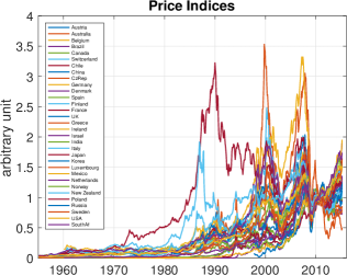
Choice has been made here to work with price indices in level, as illustrated in Fig. 1 (left). Indeed, the standard economic theory of assets prices states that all agents in equity markets have rational expectations and that markets follow random walks around trends [26]. A complementary literature further states that there is also a second category of agents whose expectations are not (or only partially) rational and thus that asset prices are affected by additional noises [27] or bubble mechanisms, i.e., temporary deviations of asset prices from fundamental values, due, for example, to liquidity trading or to waves of optimism or pessimism [28]. Thus the correlations matrices derived from long term price series in level describe the economic fundamental dimension of the integration of global equity markets, rather than its purely speculative dimension.
(a) 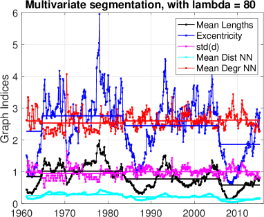 (c)
(c) 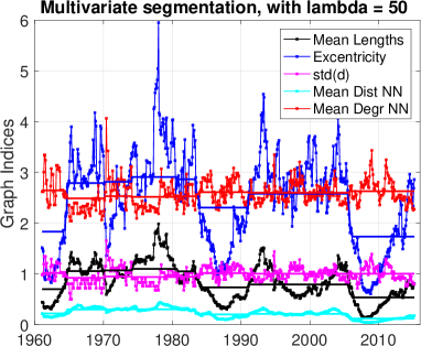
(b) 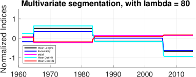 (d)
(d) 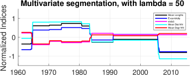
3 Method: Graph-based segmentation in eras
3.1 Step 1: Graph construction.
Instead of using directly the multivariate asset price time series or their covariance, it has been chosen to rely on the topological graph structure that accounts for the global dependence structure of multivariate data [3]. To that end, from the signed pairwise correlations between two countries and in a sliding window, the distance is computed and then used to construct a Minimal Spanning Tree (MST) on the covariance structure. This MST offers a global topological representation of the covariance, as was originally proposed in econophysics for portfolio studies [3]. It is associated with the subdominant ultrametric, providing intuitive economic interpretations because of the tree structure. An independent MST is obtained for each sliding window.
3.2 Step 2: Graph Indices.
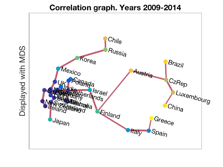
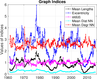
To characterize the structure of the graphs, features or indices are computed from the MST, quantifying its topology. To quantify distances, three indices are used. The mean distance to the nearest neighbors (NN) is the most basic measure. The mean length of paths (from each node to all the other nodes of the network) is a most sophisticated distance measure. The eccentricity (i.e., maximal path length) is a convenient way to display how the less integrated nodes converge. To measure connectivity, two indices are added: the standard deviation of degrees, and the mean of the degree of the nearest neighbors in the MST. Both indices are expected to increase when the structure of the network changes from a linear to a star network. All together, these indices describe if a graph is large, and if it looks more like a star or a linear structure. The complete structure can also be examined by looking at a representation of the MST (see Fig. 1 (b)).
3.3 Step 3: Multivariate joint piece-wise constant denoising.
The denoising of the time series indices is achieved by minimizing a functional form consisting of a data fidelity term balanced by a penalization term aiming to suppress spurious changes while preserving actual ones:
| (1) |
The use of total variation (or -norm) in the penalization term favors piece-wise constant solution . Its combination with a norm across components permits to favor the detection of change-point jointly across components, i.e., at the same time location. The parameter mitigates the number of change points actually produced. Intuitively, this mixed-norm penalization procedure performs a non-linear smoothing of the data, ideally smoothing when no change occur hence denoising data, while preserving actual changes. The minimization of that convex but non differentiable functional is achieved by means of proximal based primal-dual algorithms. For more details on the employed algorithm, readers are referred to [8, 29].
3.4 Visualisation of financial networks.
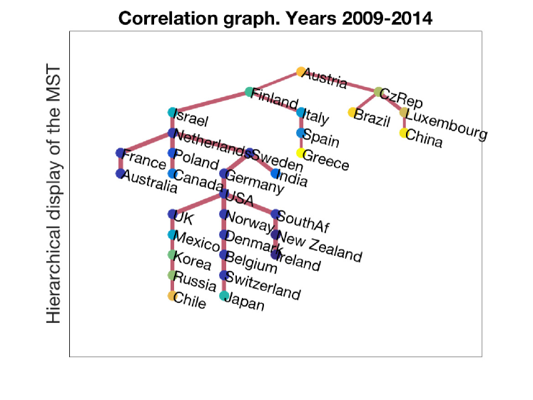
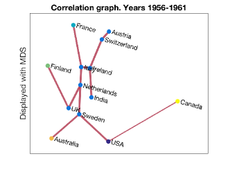
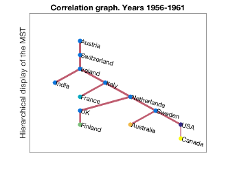
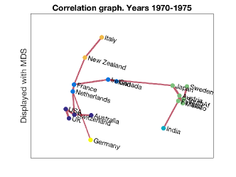
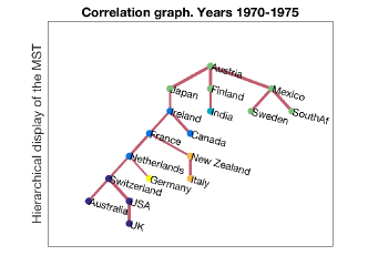
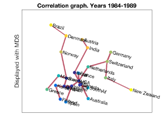
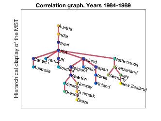
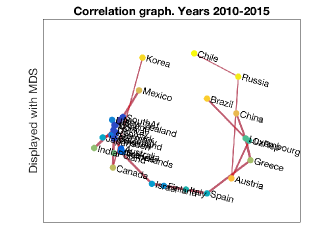
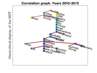
For visualisation and inspection of the results, we display in Fig. 1 (b) and later on in Fig. 3 the MST with two different techniques: first, we use classical MDS (Multi-Dimensional Scaling) [30] of the correlation distance , to embed in two dimensions the nodes of the MST. This visualization keeps all the covariance structure and reveals the distances behind the financial integration measured here. Second, we show a hierarchical view of the MST as a tree, to emphasize the relative positions of the countries. This highlights the opposition between the tree/star structure of the MST. The colors used on the nodes are derived from a hierarchical clustering using a complete linkage algorithm (as in [4]). We do not use this clustering for interpretation in the present work, as it mostly shows that classes group together neighboring nodes in the MST, as expected. The widths of the graph edges are proportional to the unsigned correlation.
(a)
(b)
(c)
(d)
4 Results and discussions
4.1 Parameter setting.
Analysis are conducted in 6-year long sliding window, chosen as a trade-off: Long enough windows ensure estimation of covariance with sufficient quality, while short windows allow for a more precise detection of change. For countries whose data is not available from the beginning, correlation is computed if data exist for at least half of the window. For the optimization involved in Step 3, no attempt to automatically tune to an optimal value has been used. Rather, has been manually adjusted to match the intuition that over the 60 years spanned by data, there should be, by nature or even definition, only a few era of stable financial integration, ranging from at least up to, say, . Still, neither the exact number of eras nor the location of the change points are chosen a priori. They constitute the outputs of the 3-step analysis procedure.
4.2 A 4-era segmentation.
A first segmentation, achieved for a large value , yields a 4-era segmentation in the time evolution of the structures of the graphs, as illustrated in Fig. 2 (a) and (b), with change points located around years: 1964, 1983 and 2007.
The change point located in 1983 is caused by a joint decrease in distance indices and increase in connectivity ones, cf. Fig. 2 (b).
From a historical economics perspective, the end of 1982 corresponds to the onset of the developing countries debt crisis.
This crisis is recognized as one of the largest financial crises of the 20th century,
resulting from the unprecedented increase in international capital flows along with the historical rise in assets prices volatility in the 1970s.
As a consequence, North-North capital flows became dominant for the next three decades, while large North-South flows were observed before 1983.
This is consistent with the lower decrease in the eccentricity of graph after the first change point, in comparison with the other distance indices.
This suggests that the convergence of developing economies is slow during the 1982-2007 subperiod.
It is also consistent with the USA becoming central in MST observed after 1983 (see Fig. 3 (c)), having then 6 edges,
as opposed to the structure of the graph observed before 1983 (Fig. 3 (a) and (b)) where it has only 2 edges and is less central, especially before 1964.
Globally, before 1983, the MST in the MDS plane (Fig. 3 (a) and (b) top) show a core of advanced economies showing moderate integration that becomes, after 1983 (Fig. 3 (c) and (d)) much more integrated in a compact core, as compared to developing or emerging economies. Indeed the distribution of the distance matrix evolves over the study period. In the beginning it is highly negatively skewed, with a predominance of distances of 0.9 to 1. Over time it becomes nearly symmetrical, with a mode of about 0.6 for the distances in the post 2000.
The change point located in 2007 is also characterized by a decrease in distance and an increase in connectivity in the graph topologies.
Eccentricity however decreases here as much as the other distance indicators (Fig. 2 (b)).
A possible economic interpretation for the date of this change may be related to the beginning of the financial crisis.
Another less trivial interpretation is that the crisis also corresponds to a return of North-South capital flows.
This return precisely results from low capital returns in advanced economies in the context of a long-lasting economic slowdown.
This economic interpretation is notably consistent with the large decrease of the eccentricity after the 2007 change point (as opposed to the 1983 change point), highlighting that the joint convergence of developing and advanced economies accelerates in the post 2007 period. MST representations also show that the USA do not maintain their 1984-89 central position (Fig. 3 (c)), and that the global structure seen in Fig. 3 (d) is a core of highly integrated nodes, with a ring
of emerging economies that are mainly located (with MDS) in the same peripheral area – whereas in the previous representation they are located in the peripheral areas of several advanced economies.
The change point located in 1964 is, we believe, mostly related to the structure of the data. Data are missing for a large number of countries before 1964, and it is thus likely that this change in the graph structures is mostly driven by the incorporation in the analysis of several new countries.
4.3 Refined segmentation.
Decreasing regularization parameter to 50 produces a segmentation in a larger number of eras, as expected. Fig. 2 right indicates that decreasing results into a further splitting of the 4-era obtained with a larger , hence yielding a hierarchical segmentation, a satisfactory outcome, not a priori imposed or induced by the analysis procedure, hence really associated to the very structure of the data. The 1964-1983 period is split into 4 different subperiods. This can be related to the large number of major economic and financial events occurring during the 1970s, such as the end of the dollar/gold convertibility in 1971, the first and second oil shocks in 1973 and 1979, the end of the Bretton Woods system in 1976 and the radical shift in the monetary policy stance of the United States in 1979. For 1983-2007, it is interesting to observe that the sub-segmentation highlights a local increase in the eccentricity measure in 1991 while the overall trend of distance indicators is decreasing over the whole study period. This is consistent with this peculiarity of the subperiod, when developing economies were left outside of international capital flows.
5 Conclusions and perspectives
The present contribution has shown a segmentation methodology, combining covariance graph constructions and analysis and state-of-the-art optimization based segmentation along time. It allows to delineate international financial integration eras using network indicators which is, to the best of our knowledge, an original contribution to the literature.
An important finding is that the analysis suggests that the main cause of the segmentation is the pattern of international capital flows. The existence or not of truly globalized capital flows, i.e., including large North-South flows, seems crucial. Regulatory shocks, in particular the end of the Bretton Woods system in 1976, appear as secondary changes in subperiod quasi-hierarchical segmentation, achieved by decreasing the penalization parameter . This result is particularly interesting insofar as the segmentation method does not necessarily induce a re-segmentation of the main segmentation when the penalization parameter decreases. Moreover, the re-segmentation precisely occurs in the 70s, where the two possible periodizations of globalization eras are superimposed.
Finally this original result is also interesting as the regulatory environment of international monetary relationships is usually considered as the most relevant delimitation of globalization eras, while the key role of the patterns of international capital flows is under-estimated. This suggests initial responses to a set of outstanding issues. Among these outstanding issues is whether the deep changes in monetary and financial institutional regimes would be the product of the changes in the structure of international capital movements. In other words, have the major institutional changes in the world since 1960 around the key break dates (1971, 1973, 1976) been dictated by changes in the structure of global financial networks? Is international financial integration the driving force of institutional change?
In future work, we plan to test the robustness of our conclusions by using various correlations measures, network representations, and indices of the graph topology.
6 Acknowledgment
This work was conducted in the CAC (Cliometrics & Complexity group) at IXXI (Institut Rhônalpin des Systèmes Complexes), and supported by the GRAPHSIP project ANR-14-CE27-0001-02, and by the ACADEMICS Grant given by the IDEXLYON project of the Université de Lyon, as part of the “Programme Investissements d’Avenir” ANR-16-IDEX-0005.
References
- [1] K. H. O’Rourke, J. G. Williamson, Globalization and history (1999).
- [2] M. Obstfeld, A. M. Taylor, Global capital markets: integration, crisis, and growth, Cambridge University Press, 2004.
- [3] R. N. Mantegna, Hierarchical structure in financial markets, The European Physical Journal B-Condensed Matter and Complex Systems 11 (1) (1999) 193–197.
- [4] C. Bastidon, A. Parent, What form did global financial integration take from 1960 to 2015? a topological analysis, Available at SSRN: https://ssrn.com/abstract=2902547 (2016).
-
[5]
M. Tumminello, F. Lillo, R. N. Mantegna,
Correlation,
hierarchies, and networks in financial markets, Journal of Economic Behavior
& Organization 75 (1) (2010) 40 – 58, transdisciplinary Perspectives on
Economic Complexity.
doi:https://doi.org/10.1016/j.jebo.2010.01.004.
URL http://www.sciencedirect.com/science/article/pii/S0167268110000077 -
[6]
D.-M. Song, M. Tumminello, W.-X. Zhou, R. N. Mantegna,
Evolution of
worldwide stock markets, correlation structure, and correlation-based
graphs, Phys. Rev. E 84 (2011) 026108.
doi:10.1103/PhysRevE.84.026108.
URL https://link.aps.org/doi/10.1103/PhysRevE.84.026108 -
[7]
Y. Chen, R. N. Mantegna, A. A. Pantelous, K. M. Zuev,
A dynamic analysis of
s&p 500, ftse 100 and euro stoxx 50 indices under different exchange rates,
PLOS ONE 13 (3) (2018) 1–40.
doi:10.1371/journal.pone.0194067.
URL https://doi.org/10.1371/journal.pone.0194067 - [8] J. Frecon, N. Pustelnik, P. Abry, L. Condat, Fast and on-the-fly approximation of multivariate total variation minimization, IEEE Transactions on Signal Processing 64 (9) (2016) 2355–2364.
-
[9]
G. Bonanno, N. Vandewalle, R. N. Mantegna,
Taxonomy of stock
market indices, Phys. Rev. E 62 (2000) R7615–R7618.
doi:10.1103/PhysRevE.62.R7615.
URL https://link.aps.org/doi/10.1103/PhysRevE.62.R7615 -
[10]
X. Xuan, K. Murphy, Modeling
changing dependency structure in multivariate time series, in: Proceedings
of the 24th International Conference on Machine Learning, ICML ’07, ACM, New
York, NY, USA, 2007, pp. 1055–1062.
doi:10.1145/1273496.1273629.
URL http://doi.acm.org/10.1145/1273496.1273629 - [11] A. J. Gibberd, J. D. B. Nelson, High dimensional changepoint detection with a dynamic graphical lasso, in: 2014 IEEE International Conference on Acoustics, Speech and Signal Processing (ICASSP), 2014, pp. 2684–2688. doi:10.1109/ICASSP.2014.6854087.
-
[12]
D. Hallac, S. Vare, S. P. Boyd, J. Leskovec,
Toeplitz inverse covariance-based
clustering of multivariate time series data, CoRR abs/1706.03161.
arXiv:1706.03161.
URL http://arxiv.org/abs/1706.03161 - [13] T. Hastie, R. Tibshirani, J. Friedman, et al., The elements of statistical learning: data mining, inference, and prediction, Springer New York, 2001.
- [14] D. Angelosante, G. B. Giannakis, Sparse graphical modeling of piecewise-stationary time series, in: 2011 IEEE International Conference on Acoustics, Speech and Signal Processing (ICASSP), 2011, pp. 1960–1963. doi:10.1109/ICASSP.2011.5946893.
-
[15]
J. G. D. Gooijer,
Detecting
change-points in multidimensional stochastic processes, Computational
Statistics & Data Analysis 51 (3) (2006) 1892 – 1903.
doi:https://doi.org/10.1016/j.csda.2005.12.004.
URL http://www.sciencedirect.com/science/article/pii/S0167947305003191 -
[16]
P. Galeano, D. Wied,
Multiple
break detection in the correlation structure of random variables,
Computational Statistics & Data Analysis 76 (Supplement C) (2014) 262 –
282, cFEnetwork: The Annals of Computational and Financial Econometrics.
doi:https://doi.org/10.1016/j.csda.2013.02.031.
URL http://www.sciencedirect.com/science/article/pii/S016794731300087X - [17] H. Yu, C. Li, J. Dauwels, Network inference and change point detection for piecewise-stationary time series, in: 2014 IEEE International Conference on Acoustics, Speech and Signal Processing (ICASSP), 2014, pp. 4498–4502. doi:10.1109/ICASSP.2014.6854453.
- [18] A. Gibberd, N. J.D.B, Estimating dynamic graphical models from multivariate time-series data: Recent methods and results, in: A. Douzal-Chouakria, J. Vilar, P. Marteau (Eds.), Advanced Analysis and Learning on Temporal Data. AALTD 2015. Lecture Notes in Computer Science, Vol. 9785, Springer, Cham, 2016.
- [19] D. Hallac, P. Nystrup, S. Boyd, Greedy Gaussian Segmentation of Multivariate Time Series, ArXiv e-printsarXiv:1610.07435.
- [20] G. Bekaert, C. R. Harvey, Capital flows and the behavior of emerging market equity returns, Tech. rep., National bureau of economic research (1998).
- [21] G. Bekaert, C. R. Harvey, R. L. Lumsdaine, Dating the integration of world equity markets, Journal of Financial Economics 65 (2) (2002) 203–247.
- [22] G. Bekaert, C. R. Harvey, C. T. Lundblad, S. Siegel, What segments equity markets?, The Review of Financial Studies 24 (12) (2011) 3841–3890.
- [23] R. E. Lucas, Why doesn’t capital flow from rich to poor countries?, The American Economic Review 80 (2) (1990) 92–96.
- [24] J. G. Williamson, Global capital markets in the long run: A review of maurice obstfeld and alan taylor’s global capital markets, Journal of economic literature 45 (2) (2007) 400–409.
- [25] R. Engle, Dynamic conditional correlation: A simple class of multivariate generalized autoregressive conditional heteroskedasticity models, Journal of Business & Economic Statistics 20 (3) (2002) 339–350.
- [26] P. A. Samuelson, Proof that properly anticipated prices fluctuate randomly, IMR; Industrial Management Review (pre-1986) 6 (2) (1965) 41.
- [27] A. Shleifer, L. H. Summers, The noise trader approach to finance, The Journal of Economic Perspectives 4 (2) (1990) 19–33.
- [28] B. Bernanke, M. Gertler, Monetary policy and asset price volatility, Tech. rep., National bureau of economic research (2000).
- [29] L. Condat, A direct algorithm for 1D total variation denoising, IEEE Signal Proc. Letters 20 (11) (2013) 1054–1057.
- [30] I. Borg, P. Groenen, Modern Multidimensional Scaling: Theory and Applications, Springer, 2005.