The nonlinear Schrödinger equation with white noise dispersion on quantum graphs

Iulian Cîmpean and Andreea Grecu ^,1

Abstract. We show that the nonlinear Schrödinger equation (NLSE) with white noise dispersion on quantum graphs is globally well-posed in $L^{2}$ once the free deterministic Schrödinger group satisfies a natural $L^{1}-L^{\infty}$ decay, which is verified in many examples. Also, we investigate the well-posedness in the energy domain in general and in concrete situations, as well as the fact that the solution with white noise dispersion is the scaling limit of the solution to the NLSE with random dispersion.

Keywords. Quantum graphs, Schrödinger operator, white noise dispersion, Strichartz estimates, nonlinear Schrödinger equation, stochastic partial differential equations, spectral theory, nonlinear fiber optics.

2010 Mathematics Subject Classification. 35J10, 34B45, 81U30, 60H15 (primary), 81Q35, 35P05, 35Q55 (secondary).

1 Introduction

The aim of this paper is to study well-posedeness results for nonlinear Schrödinger equation (NLSE) on quantum graphs, of the type

$$\mathrm{i}\dfrac{\partial u}{\partial t}+m(t)\dfrac{\partial^{2}u}{\partial x^{2}}+f(|u|^{2})u=0,$$ (1.1)

where the dispersion coefficient $m$ is randomly varying. In order to give a precise description of the goals of this work we need some preliminaries on quantum graphs, so let us postpone these to the beginning of Section 2, and discuss here some more or less general aspects concerning (1.1) that are relevant to the present work. First of all, recall that on $\mathbb{R}^{d}$, equation (1.1) is generically used to model the evolution of nonlinear dispersive waves in inhomogeneous media. It is important to mention that depending on the physical interpretation, the usual time variable $t$ and space variable $x$ can have reversed meaning. For example, when equation (1.1) describes the wave function of a particle in a Bose-Einstein condensate (also known as Gross-Pitaevskii equation), or stands as a model for superconductivity (known as Ginzburg-Landau equation), the variables $t$ and $x$ denote time and space, respectively; see [9], but also the introduction of [3] and the references therein. In contrast, when modeling the propagation of a signal in an optical fiber ($d=1$), $t$ denotes the distance along the fiber, whilst $x$ corresponds to the retarded time; see e.g. [4].

In fact, the present work is inspired by the one developed in [24] and [15] which concerns the latter physical model, so let us give more details in this direction: The following nonlinear Schrödinger equation on $\mathbb{R}$

$$\mathrm{i}\dfrac{\partial v}{\partial t}+\varepsilon m(t)\dfrac{\partial^{2}v}{\partial x^{2}}+\varepsilon^{2}|v|^{2}v=0,\quad x\in\mathbb{R},\ t>0$$ (1.2)

was considered in [24] and [15] as a model for the propagation of a signal in an optical fiber with randomly varying dispersion, where $(m(t))_{t\geq 0}$ is a centered stationary stochastic process which models the fluctuations of the dispersion, while $\varepsilon\ll 1$ controls its amplitude.

In order to understand the diffusion approximation for (1.2), i.e. the limiting case $\varepsilon\to 0$, it is convenient to consider the scaling $X(t,x)=v(\frac{t}{\varepsilon^{2}},x)$, which leads to

$$\mathrm{i}\dfrac{\partial X}{\partial t}+\dfrac{1}{\varepsilon}m(\dfrac{t}{\varepsilon^{2}})\dfrac{\partial^{2}X}{\partial x^{2}}+|X|^{2}X=0,\quad x\in\mathbb{R},\ t>0$$ (1.3)

If the following invariance principle is in force

1. $\bigg{(}\mathop{{\int_{0}^{t}}}\dfrac{1}{\varepsilon}m\bigg{(}\dfrac{s}{\varepsilon^{2}}\bigg{)}\ ds\bigg{)}_{t\geq 0}$ converges in law to a Brownian motion $(\beta(t))_{t\geq 0}$ when $\varepsilon\to 0$,

then the limit equation reads

$$dX(t)=\mathrm{i}\Delta X(t)\circ d\beta(t)+\mathrm{i}|X|^{2}X(t)\;dt,\quad t\geq 0$$ (1.4)

or in Itô form

$$dX(t)=-\frac{1}{2}\Delta^{2}X(t)\;dt+\mathrm{i}\Delta X(t)\;d\beta(t)+\mathrm{i}|X|^{2}X(t)\;dt,\quad t\geq 0$$ (1.5)

In fact, this model was first studied in [24] with a truncated nonlinearity $f(|v|^{2})v$ instead of the cubic one, where $f$ is a smooth cutoff of the identity. More precisely, it was shown that in the case of such a truncation, a contraction argument works out smoothly to prove that equations (1.3) are well posed in $L^{2}(\mathbb{R})$ and $H^{2}(\mathbb{R})$, and their solutions converge in distribution to the $L^{2}$-solution of the (truncated) limit equation (1.5), when $\varepsilon\to 0$. Also, a numerical splitting scheme was developed to simulate these solutions.

The case of full nonlinearity is much more involved, and it was treated a few years later in [15] and then in [16], for quintic nonlinearity. First of all, the varying dispersion makes the Hamiltonians associated to equations (1.2) or (1.5) to be no longer preserved, hence there are no a priori energy estimates for the solutions. Fortunately, the $L^{2}$-norm of the solution is preserved, and an $L^{2}$-approach turned out to be suitable, yet much more delicate than in the truncated case. More precisely, the key ingredient from [15], [16] consists of Strichartz type estimates obtained for the solution to the linear version of equation (1.5) (i.e. when the nonlinear term is discarded). These estimates are then employed to solve the nonlinear equation (1.5) in mild form on $L^{2}(\mathbb{R})$ (even on $H^{1}$), through a fixed point argument. We emphasize that the Strichartz estimates were obtained in [15], [16] for white noise dispersion only. They are not available for the (linear) equations (1.3) with random dispersion in general, and for this reason, for full nonlinearity, equations (1.3) can be solved only locally, up to some stopping time $\tau_{\varepsilon}$. However, it was shown in [15], [16] that these local solutions converge in law to the global solution of equation (1.5), when $\varepsilon\to 0$.

Recently, in [13] and [12], global well-posedness of nonlinear PDEs with modulated dispersion have been extended to a larger class of ”sufficiently irregular” noises. Although the results obtained in the present paper could be reconsidered under such more general noises, for simplicity we shall treat only the case of white noise dispersion.

Concerning the motivation of this paper, let us mention that in recent years there has been a growing interest in studying nonlinear Schrodinger equations on ramified structures, with different applications: condensed matter physics, nonlinear fiber optics, hydrodynamics, fluid transport, or neural networks. Such ramified structures are modeled by quantum graphs, i.e. metric graphs endowed with a self-adjoint differential operator; see e.g. [10] and the references therein. For example, in the standard case of propagation of waves in one dimensional domains, the presence of spatial point defects lead to boundary conditions and hence to a quantum graph model; see [19, 3, 22, 7] for details and further applications. Returning to the original applications of equations (1.3)-(1.5) to optical fibers as considered in [24] and [15], recall that the time and space variables $t$ and $x$ have reversed meanings. Nevertheless, in the typical situation of bimodal optical fibers where two solitons (one narrower and one wider) are coupled by two corresponding NLS equations, it is convenient to reduce the system to a single NLS equation in which the narrow soliton in the mate mode will be represented by a perturbation of a one dimensional NLS equation with an effective delta potential in the (temporal) $x$ variable; see [11, eq.(1)] and the refences therein. In this way, we are once again lead to boundary conditions at $x=0$, hence to a quantum graph model where $t$ is the distance along the fiber while $x$ corresponds to the delayed time. More complex optical networks have been recently considered in [17] or [2].

The goal of this paper is to investigate the well-posedeness of equation (1.4) (or (1.5) in equivalent Ito form), as well as the convergence of the solutions of (1.3) when $\varepsilon\to 0$, on general quantum graphs, denoted further by $\Gamma$. In the spirit of the previously mentioned applications, we emphasize that the modulation of the dispersion coefficient $(m(t))_{t\geq 0}$ in (1.4) or $(\beta(t))_{t\geq 0}$ in (1.5) may have either temporal or spatial meaning, depending on the physical system under consideration.

The rest of this paper is structured in two sections: in Section 2 we start with an overview on quantum graphs, and state the precise goals of this work. The rest and most consistent part of this section is a systematic exposition of the main results of the paper, trying to point out the specific difficulties which we deal with, in contrast to the work in [24], [15], or [16]; we structure this exposition in four subsections, as follows: Subsection 2.1 is devoted to the well-posedness of the linear equation (2.6) (Proposition 2.4) and the corresponding Strichartz estimates (Theorem 2.7); in Subsection 2.2 we obtain the well-posedness of equation (2.3) on $L^{2}(\Gamma)$ (Theorem 2.10); in Subsection 2.3, Theorems 2.11 and 2.13, we state the well posedness in the energy domain and convergence of the approximate solutions when $\varepsilon\to 0$, for truncated nonlinearities; the extension of these last two results to full nonlinearities is much more delicate, and we restrict our study to the case of star-graphs, with the mention that our strategy is general and can be applied to other situations (see Subsection 2.4, Theorems 2.17, 2.18, and 2.21). Section 3 contains the proofs of the results presented in Section 2.

2 Preliminaries on quantum graphs and the main results

First, let us give a brief overview on quantum graphs, following mainly [21] and [10]. A finite graph $\Gamma$ is a triplet $\Gamma=(V,E,\partial)$, where $V=\{v_{i}\}_{i}$ is a finite set of vertices, $E=\{e_{j}\}_{j}=:I\cup\mathcal{E}$ is a finite set of (internal, respectively external) edges that connect the vertices, and $\partial$ is a map (called orientation) which assigns to an internal edge $e\in I$ an ordered pair of vertices $\partial(e)=\{\partial^{-}(e),\partial^{+}(e)\}$, and to an external edge $e\in\mathcal{E}$ its single vertex. $\partial^{-}(e)$ and $\partial^{+}(e)$ are called the initial and the terminal vertex of the edge $e$, respectively. The graph $\Gamma$ is assumed to be connected, i.e. any two vertices can be connected by an edge w.r.t. the order given by $\partial$.

We endow the graph $\Gamma$ with the following metric structure: each internal edge $e$ is identified with an interval $[0,l_{e}]$ where zero corresponds to $\partial^{-}(e)$; similarly, an external edge corresponds to a semi line $[0,\infty)$. Based on this identification, each edge is endowed with the euclidean metric on the corresponding interval, and, in general, the distance between two points on $\Gamma$ is taken to be the length of the shortest path between them.

Function spaces on $\Gamma$. A complex valued function $f:\Gamma\to\mathbb{C}$ is regarded as a collection $f=(f_{e})_{e\in E}$, where $f_{e}:I_{e}\to\mathbb{C}$; $I_{e}=[0,l_{e}]$ or $[0,\infty)$, for all $e\in E$. We denote by $L^{p}(\Gamma)$, $1\leq p\leq\infty$, the space of all elements $f=(f_{e})_{e\in E}$ where $f_{e}\in L^{p}(I_{e})$ for all $e\in E$. $L^{p}(\Gamma)$ becomes a Banach space with respect to the norm

$$||f||^{p}_{L^{p}(\Gamma)}=\sum\limits_{e\in E}||f_{e}||^{p}_{L^{p}(I_{e})}\quad{\rm if}\quad p<\infty,\quad||f||_{L^{\infty}(\Gamma)}=\sup\limits_{e\in E}||f_{e}||_{L^{\infty}(I_{e})},$$

i.e. $L^{p}(\Gamma)=\bigoplus\limits_{e\in E}L^{p}(I_{e})$. Similarly, we consider the Sobolev spaces $W^{k,p}(\Gamma)=\bigoplus W^{k,p}(I_{e})$, $k\in\mathbb{N}^{\ast},1\leq p\leq\infty$ with the norm

$$||f||^{p}_{W^{k,p}(\Gamma)}=\sum\limits_{e\in E}||f_{e}||^{p}_{W^{k,p}(I_{e})}.$$

Remark 2.1.

Since $\Gamma$ is one dimensional, every element $f\in W^{k,p}(\Gamma)$ possesses a continuous version on each interval $I_{e}$, but there is no a priori information on how the values of $f$ at the vertices are coupled. The coupling conditions are provided by (the domain of) the heat operator, which we describe in the sequel.

Let us first consider the space of test functions $D_{0}=\bigoplus\limits_{e\in E}C_{0}^{\infty}(I_{e})$, where $C_{0}^{\infty}$ consists of infinitely differentiable functions with compact support on $\mathring{I_{e}}$, and the operator $\Delta_{\Gamma}^{0}:D_{0}\subset L^{2}(\Gamma)\to L^{2}(\Gamma)$, given by

$$(\Delta_{\Gamma}^{0}f)_{e}(x)=\dfrac{d^{2}}{dx^{2}}f_{e}(x),\;\;e\in E,x\in I_{e}.$$

By symmetry, $(\Delta_{\Gamma}^{0},D_{0})$ is a closable operator on $L^{2}(\Gamma)$, and its minimal domain, i.e. the domain of its closure, is given by $D(\Delta_{\Gamma}^{0}):=\{f\in W^{2,2}(\Gamma):f_{e}(0)=f_{e}(l_{e})=f^{\prime}_{e}(0)=f^{\prime}_{e}(l_{e})=0,\ e\in E\}$. However, the interest is to consider other coupling conditions, especially those that correspond to self-adjoint extensions of $(\Delta_{\Gamma}^{0},D_{0})$, which clearly is not the case of $(\Delta_{\Gamma}^{0},D(\Delta_{\Gamma}^{0}))$. Fortunately, the self-adjoint extensions of $(\Delta_{\Gamma}^{0},D_{0})$ can be completely characterized in terms of the coupling conditions, as follows: let $\{A_{v},B_{v}\}_{v\in V}$ be a family of matrices from $\mathbb{C}^{n_{v}\times n_{v}}$, where $n_{v}$ denotes the number of edges with common vertex $v\in V$. Let us consider the extension $\Delta_{\Gamma}$ of $(\Delta_{\Gamma}^{0},D_{0})$, with domain

$$D(\Delta_{\Gamma}):=\{f\in H^{2}(\Gamma):\ A_{v}\overline{f_{v}}+B_{v}\overline{f^{\prime}_{v}}=0,\ v\in V\}$$

where $\overline{f_{v}}=(f_{e}(v))_{e\in E}$ and $\overline{f^{\prime}_{v}}=(f^{\prime}_{e}(v))_{e\in E}$ are column vectors.

Now we can recall the following well known characterization.

Theorem 2.2 (cf. [21]).

$(\Delta_{\Gamma},D(\Delta_{\Gamma}))$ is self-adjoint if and only if the following conditions are satisfied:

1. The concatenated matrix $(A_{v},B_{v})$ has maximal rank, $n_{v}$;

2. $A_{v}B^{{\dagger}}_{v}$ is self-adjoint, where $B^{{\dagger}_{v}}$ is the adjoint transpose of $B_{v}$.

We emphasize that the coupling matrices $A_{v},B_{v}$ are not unique (but merely modulo an invertible matrix). There is another characterization due to [10, Theorem 1.4.4], according to which the operator $\Delta_{\Gamma}$ is self-adjoint if and only if for every vertex $v$ of degree $d_{v}$, there are three unique orthogonal (and mutually orthogonal) projectors $P_{D,v},P_{N,v}$, and $P_{R,v}=I-P_{D,v}-P_{N,v}$ acting on $\mathbb{C}^{d_{v}}$, and $\Lambda_{v}$ invertible and self-adjoint acting on $P_{R,v}\mathbb{C}^{d_{v}}$, such that the boundary values of $f$ satisfy

$$\begin{cases}P_{D,v}\overline{f_{v}}=0,&"Dirichlet\,Part"\\ P_{N,v}\overline{f^{{}^{\prime}}_{v}}=0,&"Neumann\,Part"\\ P_{R,v}\overline{f^{{}^{\prime}}_{v}}=\Lambda_{v}P_{R,v}\overline{f_{v}},&"Robin\,Part"\\ \end{cases}.$$

The quadratic form $\mathcal{E}$ associated to $\Delta_{\Gamma}$ is given by

$$\mathcal{E}(f,f)=\sum_{j=1}^{|E|}\int_{e_{j}}|f^{\prime}_{j}(x)|^{2}\,dx+\sum_{v\in V}<\Lambda_{v}P_{R,v}f(v),P_{R,v}f(v)>\;\;\mbox{for all }f\in D(\mathcal{E});$$

$$D(\mathcal{E}):=\{f\in W^{1,2}(\Gamma)\,:\,P_{D,v}f(v)=0\;\mbox{ for all }v\in V\}.$$ (2.1)

We will frequently employ the following equivalence of norms.

Proposition 2.3 (cf. [10], p. 23).

There exists $M>0$ such that for any $f\in D(\mathcal{E})$, the norm $\|\cdot\|_{D(\mathcal{E})}$ given by

$$\|f\|_{D(\mathcal{E})}:=\sqrt{M\|f\|^{2}_{L^{2}(\Gamma)}+\mathcal{E}(f,f)}$$ (2.2)

is well defined and equivalent to $\|\cdot\|_{W^{1,2}(\Gamma)}$. In particular, $(D(\mathcal{E}),\|\cdot\|_{D(\mathcal{E})})$ is a Hilbert space.

From now on we assume that $(\Delta_{\Gamma},D(\Delta_{\Gamma})$ is a self-adjoint extension of $(\Delta^{0}_{\Gamma},D(\Delta^{0}_{\Gamma})))$ with local coupling conditions $\{A_{v},B_{v}\}_{v\in V}$. By $\mathrm{e}^{\mathrm{i}t\Delta_{\Gamma}}$ we denote the strongly continuous group of izometries on $L^{2}(\Gamma)$ generated by $\mathrm{i\Delta_{\Gamma}}$.

Main goals. For the rest of the paper, $\beta:=(\beta(t))_{t\geq 0}$ denotes a standard 1-dimensional Brownian motion on a filtered probability space $(\Omega,\mathcal{F},\mathcal{F}_{t},\mathbb{P})$ which satisfies the usual hypotheses. We point out that throughout, $(\beta(t))_{t\geq 0}$ could be replaced by $(\beta(t)+\mu t)_{t\geq 0}$ for some constant $\mu\in\mathbb{R}$.

The first main aim is to investigate the well-posedeness in $L^{2}(\Gamma)$ and $D(\mathcal{E})$ of the following nonlinear Schrödinger equation with white noise dispersion, on $\Gamma$:

$$\left\{\begin{array}[]{lll}dX(t)=-\frac{1}{2}\Delta_{\Gamma}^{2}X(t)\;dt+i\Delta_{\Gamma}X(t)\;d\beta(t)+i|X|^{2\sigma}X(t)\;dt,&t\in[0,\infty)\\[5.0pt] X(0)=X_{0}.\\ \end{array}\right.$$ (2.3)

In fact, as in [15], the strategy is to tackle (2.3) in mild form:

$$X(t)=S_{\beta}(t,0)X_{0}+\mathrm{i}\int_{0}^{t}S_{\beta}(t,s)|X(s)|^{2\sigma}X(s)\;ds,\quad t\geq 0,\ \mathbb{P}\mbox{-a.s.}$$ (2.4)

where $S_{\beta}(\cdot,s)$ (see Subsection 2.1) gives the solution to the linear equation, starting at time $s\geq 0$. We emphasize that the sign in front of the nonlinearity is not important, since $-\beta$ is still a Brownian motion.

The second aim is to study the convergence of the (local) solutions of

$$\begin{cases}\dfrac{dX(t)}{dt}=\mathrm{i}\dfrac{1}{\varepsilon}m\bigg{(}\dfrac{t}{\varepsilon^{2}}\bigg{)}\Delta_{\Gamma}X(t)+\mathrm{i}|X|^{2\sigma}X(t)=0,&t>0,\ \mbox{ on }\Gamma\\ X(0)=X_{0}\end{cases},$$ (2.5)

to the solution of (2.3), when $\varepsilon\to 0$, provided that the process $m$ satisfies (H.0).

2.1 The linear stochastic equation and Strichartz type estimates

As in [15], the key ingredient to prove the well-posedness of (2.4) is the Strichartz type estimates for the solution to the linear Schrödinger equation with white noise dispersion:

$$\left\{\begin{array}[]{lll}dX(t)=-\frac{1}{2}\Delta_{\Gamma}^{2}X(t)\;dt+\mathrm{i}\Delta_{\Gamma}X\;d\beta(t),&t\geq s\\[5.0pt] X(s)=X_{s}\\ \end{array}\right.$$ (2.6)

Recall that on $\mathbb{R}$, the solution to (2.6) can be explicitly obtained by Fourier transform (see [24] and [15]), and it is given by

$$S_{\beta}(t,s)X_{s}(\omega):={\mathrm{e}^{\mathrm{i}[\beta(t)-\beta(s)](\omega)\Delta_{\Gamma}}}X_{s}(\omega)\;\;\mbox{ for }s\leq t,\omega\in\Omega.$$ (2.7)

Although Fourier transform is no longer available on $\Gamma$, we can use spectral arguments to rigorously show that $S_{\beta}(t,s)$ is well-defined and gives the solution to (2.6). More precisely, we have:

Proposition 2.4.

Let $s\geq 0$ and assume that $X_{s}\in D(\Delta_{\Gamma}^{2})$ $\mathbb{P}$-a.s. Then $(S_{\beta}(t,s)X_{s})_{t\geq s}$ given by (2.7) is the (pathwise) unique strong solution to (2.6), with paths in $C([s,\infty),D(\Delta_{\Gamma}^{2}))$ a.s. In particular, $|S_{\beta}(t,s)X_{s}|_{L^{2}}=|X_{s}|_{L^{2}}\ for\ all\ t\geq s\mbox{ a.s.}$

Remark 2.5.

In the previous proposition, if $X_{s}\in D(\Delta_{\Gamma}^{2})$ is deterministic, then the fact that $S(\cdot,s)X_{s}$ is a solution would follow directly by Itô formula on Hilbert spaces (see e.g. [14, 23]), since $F:\mathbb{R}\rightarrow L^{2}(\Gamma)$, $F(t)={\mathrm{e}^{\mathrm{i}t\Delta_{\Gamma}}X_{s}}$ is twice Frechet differentiable. However, for the sake of the mild formulation (2.4), it is necessary to allow random initial data $X_{s}$, and we do this rigorously in Proposition 2.4 is to do this rigorously. ensures that $S(\cdot,s)X_{s}$ remains the solution to (2.6) also for random initial data.

In orther to get the desired Strichartz estimates, we point out that in the case $\Gamma=\mathbb{R}$, the key starting point in [15] is the dispersive estimate $|e^{it\Delta}|_{L^{1}(\mathbb{R})\to L^{\infty}(\mathbb{R})}\lesssim|t|^{-1/2},t\in\mathbb{R}^{\ast}$. Such an estimate on $\Gamma$ is verified in few situations, mainly because of the presence of nonempty point spectrum, and it turns out that the following general hypothesis is much more convenient:

1. The number of eigenvalues of $-\Delta_{\Gamma}$, counting their multiplicities, is at most finite, and there exists a constant $C>0$ such that

   $$\|{\mathrm{e}^{\mathrm{i}t\Delta_{\Gamma}}P_{c}}u_{0}\|_{L^{\infty}(\Gamma)}\leq C\dfrac{1}{\sqrt{|t|}}\ \|u_{0}\|_{L^{1}(\Gamma)},\quad\text{for all }u_{0}\in L^{1}(\Gamma)\cap L^{2}(\Gamma)\text{ and }t\neq 0,$$ (2.8)

   where $P_{c}=I-P_{p}$, and $P_{p}$ is the orthogonal projection onto the linear span of the eigenfunctions, in $L^{2}(\Gamma)$.

In subsections 2.4 and 2.5 we discuss general and concrete situations when hypothesis (H.1) is fulfilled.

Definition 2.6.

Following [15], an exponent pair $(r,p)$ is called admissible if $r=\infty,p=2$ or $2\leq r,p<\infty$ and $\frac{2}{r}+\frac{1}{p}>\frac{1}{2}$.

In the sequel, in order to lighten the notations, we shall often write $L^{r}_{\omega}L^{r}_{[s,s+T]}L^{p}_{x}$ instead of $L^{r}(\Omega;L^{r}([s,s+T];L^{p}(\Gamma)))$.

Extending [15, Propositions 3.10 and 3.11], we get the following Strichartz estimates.

Theorem 2.7.

Assume that (H.1) is satisfied. Let $T>0$, $s\geq 0$, and $(r,p)$ an admissible exponent pair. Then

(i)

$${\big{\|}S_{\beta}(\cdot,s)X_{s}\big{\|}_{L^{r}_{\omega}L^{r}_{[s,s+T]}L^{p}_{x}}\leq c_{r,p}\;T^{\beta/2}\;\|X_{s}\|_{L^{r}_{\omega}L^{2}_{x}}},\ \text{ with }\beta=\tfrac{2}{r}-\tfrac{1}{2}(\tfrac{1}{2}-\tfrac{1}{p});$$

(ii) Let $(\gamma,\delta)$ be another admissible pair such that $\frac{1}{\gamma}=\frac{1-\lambda}{r},\frac{1}{\delta}=\frac{\lambda}{2}+\frac{1-\lambda}{p}$ for some $\lambda\in[0,1]$.

(ii.1) If $\max\{\rho,\rho^{\prime}\}\leq r$, $\overline{\beta}=\beta(1-\frac{\lambda}{2})$, and $f$ is predictable, then

$$\qquad\qquad\qquad\bigg{\|}\int_{s}^{\cdot}S_{\beta}(\cdot,\sigma)f(\sigma)d\sigma\bigg{\|}_{L^{\rho}_{\omega}L^{r}_{[s,s+T]}L^{p}_{x}}\leq c_{r,p,\gamma,\delta,\rho}\;T^{\overline{\beta}}\;\big{\|}f\big{\|}_{L^{\rho}_{\omega}L^{\gamma^{\prime}}_{[s,s+T]}L^{\delta^{\prime}}_{x}};$$

(ii.2) If $r^{\prime}\leq\rho\leq r$, then

$$\qquad\qquad\qquad\bigg{\|}\int_{s}^{\cdot}S_{\beta}(\cdot,\sigma)f(\sigma)d\sigma\bigg{\|}_{L^{\rho}_{\omega}L^{\gamma}_{[s,s+T]}L^{\delta}_{x}}\leq c_{r,p,\gamma,\delta,\rho}\;T^{\overline{\beta}}\;\big{\|}f\big{\|}_{L^{\rho}_{\omega}L^{r^{\prime}}_{[s,s+T]}L^{p^{\prime}}_{x}},$$

2.2 Well-posedeness of equation (2.4) on $L^{2}(\Gamma)$

As already mentioned, the idea to solve (2.4) on $L^{2}(\Gamma)$ is to apply the Banach fixed point theorem on some convenient space, based on the estimates obtained in Theorem 2.7. However, looking at these estimates, one can notice that the smoothing effect is present in space-time, but not in $\Omega$. For this reason, as in [15], we first need to consider a truncation in the $L^{r}_{[s,s+t]}L^{p}_{x}$-spaces, as follows: let $\theta\in C_{0}^{\infty}(\mathbb{R})$ such that $\theta=1$ on $[0,1]$ and $\theta=0$ on $[2,\infty)$. For $X\in L^{r}_{\rm loc}([s,\infty),L^{p}_{x})$ a.s., $R\geq 1$ and $t\geq 0$, we set

$$\theta_{R}^{s}(X)(t):=\theta\bigg{(}\frac{|X|_{L^{r}_{[s,s+t]}L^{p}_{x}}}{R}\bigg{)}.$$ (2.9)

For $s=0$, we set $\theta_{R}:=\theta^{0}_{R}$.

We consider the following truncated version of (2.6)

$$\left\{\begin{array}[]{lll}dX^{R}=-\frac{1}{2}\Delta_{\Gamma}^{2}X^{R}\;dt+\mathrm{i}\Delta_{\Gamma}X^{R}\;d\beta(t)+\mathrm{i}\theta_{R}(X^{R})|X^{R}|^{2\sigma}X^{R}\;dt,&t\in[0,T]\\[5.0pt] X^{R}(0)=X_{0}\\ \end{array}\right.$$ (2.10)

or in mild form:

$$X^{R}(t)=S_{\beta}(t,0)X_{0}+\mathrm{i}\int_{0}^{t}S_{\beta}(t,s)\theta_{R}(X^{R})(s)|X^{R}(s)|^{2\sigma}X^{R}(s)\;ds,\quad t\in[0,T]\;a.s.$$ (2.11)

Throughout, by $L^{r}_{\mathcal{P}}(\Omega\times[0,T];L^{p}_{x})$ we denote the predictable processes from $L^{r}(\Omega\times[0,T];L^{p}_{x})$.

Theorem 2.8.

Assume that (H.1) is satisfied and let $\sigma<2$, $p=2\sigma+2$ and $(r,p)$ be an admissible exponent pair. Then for any $\mathcal{F}_{0}$-measurable $X_{0}\in L^{r}_{\omega}L^{2}_{x}$ there exists a unique solution $X^{R}$ to (2.11) such that $X^{R}\in L^{r}_{\mathcal{P}}(\Omega\times[0,T];L^{p}_{x})$ for any $T>0$, and has paths in $C(\mathbb{R}_{+},L^{2}_{x})$ a.s. Moreover, a.s. $|X^{R}(t)|_{L^{2}_{x}}=|X_{0}|_{L^{2}_{x}},\;t\geq 0$ and $X^{R}\in L^{\rho}_{[0,T]}L^{q}_{x}$ a.s. for any $T>0$, $\rho\leq r$ and $(\rho,q)$ admissible.

Remark 2.9.

In [15], where $\Gamma=\mathbb{R}$, the proof of Theorem 2.8 is based on a regularization of the solution to (2.10) obtained at a first stage by a fixed point argument on $L^{r}_{\mathcal{P}}(\Omega\times[0,T];L^{p}_{x})$, using a cutoff in the Fourier space. Since such a regularization cannot be performed on $\Gamma$, we have to use different arguments for the proof, which turn out to be simpler and more general; see Section 3.

Based on Theorem 2.8, the arguments from [15], Section 5, work without any change to get the $L^{2}(\Gamma)$-well-posedness of (2.4). Although we resume only to the statement (see Theorem 2.10 below) and skip its proof, let us briefly explain how it can be worked out. First of all, uniqueness follows by Theorem 2.8. Then, using again Theorem 2.8, let $X^{R}_{n}$, $n\geq 0$ be the global solutions to (2.11), obtained recursively for initial data $X_{\tau_{R}^{n}}$ where $\tau_{R}^{0}=0$ and

$$\tau_{R}^{n}:=\inf\{t\geq 0:|X^{R}_{n}|_{L^{r}_{[0,t]}L^{p}_{x}}\geq R\}\;\;\mbox{ for all }n\geq 0.$$

By superposing $X_{\tau_{R}^{n}}1_{[0,\tau_{R}^{n}]}$ for all $n\geq 0$, we get a strong Markov solution to (2.4) on $[0,\tau)$ where $\tau=\sum\limits_{n=0}^{\infty}\tau_{R}^{n}$. To make sure that $\tau=\infty$ a.s., it is sufficient to show that there exists $\varepsilon>0$ s.t. $\lim\limits_{N}\lim\limits_{M}\mathbb{P}(\tau_{R}^{n}\leq\varepsilon\mbox{ for all }N\leq n\leq M)=0$. But $\mathbb{P}(\tau_{R}^{n}\leq\varepsilon\mbox{ for all }N\leq n\leq M)=\mathbb{E}\big{\{}[\prod\limits_{n=N}^{M-1}1_{\tau_{R}^{n}\leq\varepsilon}]\;\mathbb{P}(\tau_{R}^{M}\leq\varepsilon|\mathcal{F}_{\tau_{R}^{0}+\cdots+\tau_{R}^{M-1}})\big{\}}$. Hence, it is sufficient to show that there exist $\varepsilon,R>0$ s.t. $\mathbb{P}(\tau_{R}^{M}\leq\varepsilon|\mathcal{F}_{\tau_{R}^{0}+\cdots+\tau_{R}^{M-1}})\leq\frac{1}{2}$ for all $M$, and this can indeed be obtained by the Strichartz estimates in Theorem 2.7, the conservation of the $L^{2}$-norm obtained in Theorem 2.8, and the strong Markov property; for more details see [15, Lemma 5.1] and the discussion right after.

Consequently, we obtain:

Theorem 2.10.

Assume that (H.1) is satisfied, and let $\sigma<2$ and $r$ such that $2\sigma+2\leq r<\frac{4(\sigma+1)}{\sigma}$. Then for any $X_{0}\in L^{2}(\Gamma)$, there exists a unique solution to (2.4) which has paths in $C([0,\infty),L^{2}(\Gamma))\,a.s.$. In addition, $|X(t)|_{L^{2}_{x}}=|X_{0}|_{L^{2}_{x}},\;t\geq 0$ and $X\in L^{\rho}_{[0,T]}L^{q}_{x}$ a.s. for any $T>0$, $\rho\leq r$ and $(\rho,q)$ admissible.

2.3 Well-posedeness of (2.5) for truncated nonlinearities and convergence when $\varepsilon\to 0$

In this section our aim is to extend the results from [24] to quantum graphs. More precisely, let $\theta$ be the function from the beginning of Subsection 2.2, $\sigma\geq\frac{1}{2},R>0$ and consider the function $F:\mathbb{C}\rightarrow\mathbb{C}$ given by

$$F(x):=|x|^{2\sigma}x\theta(|x|^{2}/R),$$

which is from $C^{1}_{c}$ with Lipschitz derivative. Then, the equations we deal with in this subsection are the truncated versions of (2.5), namely

$$\begin{cases}\mathrm{i}\dfrac{du}{dt}+\dfrac{1}{\varepsilon}m\bigg{(}\dfrac{t}{\varepsilon^{2}}\bigg{)}\Delta_{\Gamma}u+F(u)=0,&x\in\Gamma,\ t>0\\ u(0)=u_{0},&x\in\Gamma\end{cases},$$ (2.12)

with the corresponding limiting equation

$$\begin{cases}udt=\mathrm{i}\Delta_{\Gamma}ud\beta-\dfrac{1}{2}\Delta^{2}_{\Gamma}udt+\mathrm{i}F(u)dt,&x\in\Gamma,\ t>0\\ u(0)=u_{0},&x\in\Gamma\end{cases},$$ (2.13)

We recall that we perform such a truncation because there are no Strichartz estimates available for general varying dispersion as for the white noise case from Subsection 2.1; as a consequence, (2.5) will be solved only locally.

First, we prove well-posedness in $C([0,T],L^{2}(\Gamma))$ and in $C([0,T],D(\mathcal{E}))$ for the equation in mild form

$$u_{n}(t)=S_{n}(t,0)u_{0}+\mathrm{i}\int_{0}^{t}S_{n}(t,s)F(u_{n})(s)\,ds,$$ (2.14)

for any $n\in C([0,T],\mathbb{R})$, where $S_{n}(t,s):=\mathrm{e}^{\mathrm{i}[n(t)-n(s)]\Delta_{\Gamma}}$.

We need to consider the following stability of $D(\mathcal{E})$ under nonlinearity:

1. $\!\begin{aligned} \text{If }u\in D(\mathcal{E}),\text{ then }F(u)\in D(\mathcal{E}).\end{aligned}$

Theorem 2.11.

Let $T>0$ and $n\in C([0,T],\mathbb{R})$. Then, for any initial data $u_{0}\in L^{2}(\Gamma)$, there exists a unique solution $u_{n}\in C([0,T],L^{2}(\Gamma))$ to (2.14).

Moreover, if $u_{0}\in D(\mathcal{E})$ and $F$ satisfies (H.2), then $u_{n}\in C([0,T],D(\mathcal{E}))$.

Remark 2.12.

In particular, Theorem 2.11 applies to (2.12) and (2.13) for $n(t)=\int_{0}^{t}\frac{1}{\varepsilon}m\big{(}\frac{s}{\varepsilon^{2}}\big{)}\,ds$, and for $n(t)=\beta(t)$, respectively, $t\geq 0$.

The main result of this section is the following.

Theorem 2.13.

If (H.0) and (H.2) hold, then the mild solutions $(u_{\varepsilon})_{\varepsilon>0}$ of (2.12) converge in law to the mild solution $u$ of (2.13) when $\varepsilon\to 0$, on $C([0,T],D(\mathcal{E}))$.

2.4 Well-posedness in $D(\mathcal{E}_{\star})$ for full nonlinearity and convergence of the approximate solutions: the case of star-graphs

Concerning the well-posedeness of (2.4) in the energy domain $D(\mathcal{E})$ given by (2), let us mention once again that the dispersion destroys the conservation in time of the energy $\mathcal{E}(X(t),X(t))-\frac{1}{2\sigma+2}\|X(t)\|^{2\sigma+2}_{L^{2\sigma+2}(\Gamma)}$, hence an approach as in e.g. [18, Theorem C] (more precisely, see Proposition 3.7) or [3] is not suitable. On $\mathbb{R}$, the well-posedeness in $W^{1,2}(\mathbb{R})$ has been obtained in [15] based on the Strichartz estimates and the fact that the first derivate operator commutes with the deterministic Schrödinger group, i.e. $\frac{d}{dx}e^{it\Delta}=e^{it\Delta}\frac{d}{dx}$. However, the situation changes drastically in our case because such a commuting property simply does not hold. To overcome this problem, the strategy is to employ spectral arguments and explicit heat kernels formulas in order to be able to partially commute $\frac{d}{dx}$ with $e^{it\Delta_{\Gamma}}$, with the price of a reminder part which hopefully is also smoothing. Since it may be too difficult to get such formulas for quantum graphs in general, we restrict our analysis to the case of star graphs, with the emphasis that our strategy is a general one and could be applied to other types of graphs. So, our main concern in this section is to prove well-posedness of equation (2.4) in the energy domain $D(\mathcal{E}_{\star})$ described in (2), where $\mathcal{E}_{\star}$ denotes the form associated to a self-adjoint Hamiltonian on a star-graph, as well as the convergence of the solutions of (2.5), when $\varepsilon\to 0$. We recall that a star-graph $\Gamma_{\star}$, is a metric graph that consists of a finite number $n\in\mathbb{N}^{*}$ of infinite length edges attached to a single common vertex, with each edge being identified with a copy of the positive real axis, $[0,\infty)$.

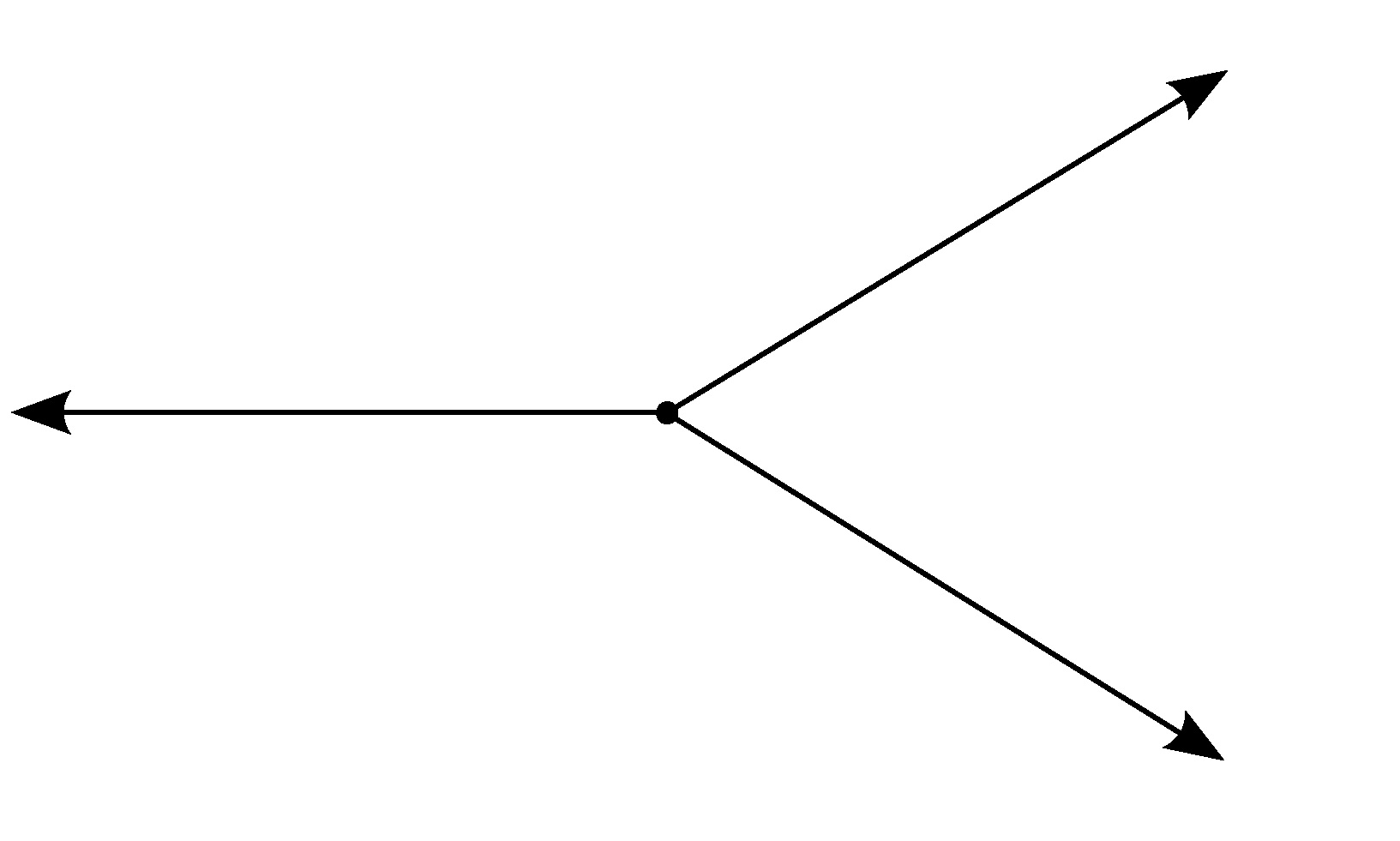
Figure 1: Star-graph, $\Gamma_{\star}$.

We denote by $H_{\star}:=-\Delta_{\Gamma_{\star}}(A,B)$ the Hamiltonian on $\Gamma_{\star}$, with $A$ and $B$ satisfying the hypotheses of Theorem 2.2.

Proposition 2.14.

Condition (H.1) is fulfilled for $H_{\star}$. In particular, Theorem 2.10 applies.

Proof.

The estimate (2.8) is one of the main results in [18], more precisely, Theorem A. The second part of (H.1) follows by [21, Identity (3.1) and Theorem 3.7], according to which there are no positive eigenvalues of $H_{\star}$ and the number of negative ones is finite counting their multiplicities and equals precisely the number of positive eigenvalues of $AB^{{\dagger}}$, denoted further by $n_{+}(AB^{{\dagger}})$. ∎

In fact, the work from [18] extends to general coupling conditions the dispersive properties obtained in [1] for the following three particular couplings (see [10] for details and physical meaning):

1. The Kirchhoff Hamiltonian $\Delta^{K}_{\Gamma}$ with domain

$$\mathcal{D}(\Delta_{\Gamma})=\big{\{}\psi\in H^{2}(\Gamma):\ \psi_{i}(0)=\psi_{j}(0),\ 1\leq i,j\leq n,\ \sum_{j=1}^{n}\psi^{\prime}_{j}(0_{+})=0\big{\}};$$

2. The $\delta$ (Delta) Hamiltonian $\Delta^{\delta}_{\Gamma}$ with domain

$$\mathcal{D}(\Delta^{\delta}_{\Gamma})=\big{\{}\psi\in H^{2}(\Gamma):\ \psi_{i}(0)=\psi_{j}(0),\ 1\leq i,j\leq n,\ \sum_{j=1}^{n}\psi^{\prime}_{j}(0_{+})=\alpha\psi_{1}(0)\big{\}},\alpha\in\mathbb{R};$$

3. The $\delta^{\prime}$ (Delta-prime) Hamiltonian $\Delta^{\delta^{\prime}}_{\Gamma}$ with domain

$$\mathcal{D}(\Delta^{\delta^{\prime}}_{\Gamma})=\big{\{}\psi\in H^{2}(\Gamma):\ \psi^{\prime}_{i}(0_{+})=\psi^{\prime}_{j}(0_{+}),\ 1\leq i,j\leq n,\ \sum_{j=1}^{n}\psi_{j}(0)=\beta\psi_{1}(0)\big{\}},\beta\in\mathbb{R}.$$

To be more precise, in [1] $\alpha$ and $\beta$ are assumed to be strictly positive, and in these cases, (H.1) is satisfied for $\mathrm{e}^{\mathrm{i}t\Delta}$ instead of $\mathrm{e}^{\mathrm{i}t\Delta}P_{c}$.

Proposition 2.15.

For Kirchhoff and $\delta-$couplings, condition (H.2) is also satisfied. In particular, Theorems 2.11 and 2.13 also apply.

Proof.

It is clear since $D(\mathcal{E}_{\star}):=\{\psi\in W^{1,2}(\Gamma)\,:\,\psi_{i}(0)=\psi_{j}(0),\ 1\leq i,j\leq n\}$ in both cases. ∎

Coupling conditions with no Robin part.

The following commuting formula will be crucially used and it could be itself of general interest.

Proposition 2.16.

If $P_{R}=0$, i.e. there is no Robin coupling, and $v\in D(\mathcal{E}_{\star})$, then

$$\partial_{x}(\mathrm{e}^{-\mathrm{i}tH_{\star}}v(x))=\mathrm{e}^{-\mathrm{i}tH_{\star}}P_{c}v^{\prime}(x)+2\mathrm{e}^{\mathrm{i}t\Delta_{\mathbb{R}}}\widetilde{v^{\prime}}(x)+\sum_{l=1}^{n_{+}(AB^{{\dagger}})}\langle v,\varphi_{l}\rangle\mathrm{e}^{-\mathrm{i}t\lambda_{l}}\varphi_{l}^{\prime}(x),$$ (2.15)

where $\mathrm{e}^{\mathrm{i}t\Delta_{\mathbb{R}}}$ is the unitary group generated by the free Schrödinger operator on $\mathbb{R}$, $\{(\lambda_{l},\varphi_{l})\}_{l}$ are the eigencouples of $H_{\star}$ and $\widetilde{v^{\prime}}=(v^{\prime}_{1},v^{\prime}_{2},\dots,v^{\prime}_{n})^{T}$, with

$$\widetilde{v^{\prime}_{j}}(x)=\begin{cases}v^{\prime}_{j}(x),&x\in[0,\infty)\\ 0,&x\in(-\infty,0)\end{cases}.$$ (2.16)

We have the following well-posedness result.

Theorem 2.17.

Let $\sigma<2$, $p=2\sigma+2$ and $(r,p)$ an admissible exponent pair. If (H.2) holds and $P_{R}=0$, then, for any $\mathcal{F}_{0}$-measurable $X_{0}\in L^{r}_{\omega}D(\mathcal{E}_{\star})$ there exists a unique solution $X$ to (2.4) with $a.s$ paths in $C(\mathbb{R_{+}},D(\mathcal{E_{\star}}))$.

Finally, let us consider the approximate equations (2.5), for which we emphasize that merely local solutions can be obtained, due to Theorem 2.11. Nevertheless, as in [16], the global well-posedness in the energy domain of the limiting equation (2.3) allows us to prove that the local solutions of (2.5) converge to the desired limit. More precisely, we have:

Theorem 2.18.

Let $\sigma\in[1/2,2)$ and assume that (H.2) holds and $P_{R}=0$. If $X_{0}\in D(\mathcal{E}_{\star})$, then for every $\varepsilon>0$ there exists a unique (mild) solution $X_{\varepsilon}$ to (2.5) with continuous paths in $D(\mathcal{E}_{\star})$, which is defined on a random time interval $[0,\tau_{\varepsilon})$. Moreover, for any $T>0$

$$\lim\limits_{\varepsilon\to 0}\mathbb{P}([\tau_{\varepsilon}<T])=0$$

and the process $X_{\varepsilon}\mathbbm{1}_{[0,\tau_{\varepsilon})}$ converges in law to the solution $X$ of (2.4) when $\varepsilon\to 0$, on $C([0,T];D(\mathcal{E}_{\star}))$.

Remark 2.19.

In the cases of Kirchhoff and Dirichlet boundary conditions, (H.2) holds and $P_{R}=0$, hence Theorems 2.17 and 2.18 apply.

A case of non-zero Robin part: $\delta-$type condition. If $P_{R}\neq 0$, we do not know if $\mathrm{e}^{\mathrm{i}t\Delta_{\Gamma}}$ has smoothing effect on $L^{r}_{t}W^{1,p}_{x}$ spaces in general. Nevertheless, we have at least one example of interest where $P_{R}=0$, namely $\delta-$ coupling conditions, for which a formula similar to (2.15) holds, and it ensures the desired smoothing effect.

Proposition 2.20.

For $\delta-$coupling conditions, the following holds for all $v\in D(\mathcal{E}_{\star})$:

$$\partial_{x}(\mathrm{e}^{-\mathrm{i}tH_{\star}}v(x))=\mathrm{e}^{-\mathrm{i}tH_{\star}}P_{c}v^{\prime}(x)+2\mathrm{e}^{\mathrm{i}t\Delta_{\mathbb{R}}}\widetilde{v^{\prime}}(x)+\sum_{l=1}^{n_{+}(AB^{{\dagger}})}\langle v,\varphi_{l}\rangle\mathrm{e}^{-\mathrm{i}t\lambda_{l}}\varphi_{l}^{\prime}(x)+\dfrac{2\alpha v_{1}(0)}{n}\mathrm{e}^{\mathrm{i}t\Delta_{\mathbb{R}}}\varphi(x),$$ (2.17)

with $\{(\lambda_{l},\varphi_{l})\}_{l}$ the eigencouples of $H_{\star}$, $\psi(y):=\mathrm{e}^{\frac{\alpha}{3}y}\mathbbm{1}_{(-\infty,0]}(y)$ and $\widetilde{v^{\prime}}$ as in (2.16).

Since $D(\mathcal{E})$ is continuously embedded in $L^{\infty}(\Gamma)$, we can bound $|u_{0,1}(0)|$ with $\|u_{0}\|_{D(\mathcal{E})}$,and the proofs of Theorems 2.17 and 2.18 can be easily adjusted to get:

Theorem 2.21.

The conclusions of Theorems 2.17 and 2.18 are valid for $\delta-$coupling conditions.

2.5 Further examples

First of all, we would like to emphasize that the results from Subsection 2.2 hold for self-adjoint operators which satisfy (H.1), on any $L^{2}-$space, i.e. the metric graph structure was not crucial for those results. For example, in [8, Theorem 1.2] it was shown that (H.1) is satisfied with $P_{c}=Id$ for $H=\frac{\partial}{\partial x}(a(x)\frac{\partial}{\partial x})$ on $L^{2}(\mathbb{R})$, with $a\in BV(\mathbb{R})$, bounded, such that $Var(log(a))<2\pi$. In particular, Theorem 2.10 applies to prove well-posedness on $L^{2}(\mathbb{R})$ for equation (2.4) with $\Delta_{\Gamma}$ replaced by $H$.

In the sequel, we present several examples of coupling conditions which induce self-adjoint extensions of the Laplacian $\Delta_{\Gamma}$ on different types of metric graphs $\Gamma$, for which the $L^{1}-L^{\infty}$ dispersive estimate (H.1) and stability condition (H.2) hold, other than star-graphs, the latter being already extensively studied in Subsection 2.4.

2.5.1 Simple graphs with internal edges

We include here the case of the Schrödinger group on the real line with several point defects, which can be regarded as simple graphs with a finite number $n\in\mathbb{N}^{*}$ of edges, with particular self-adjoint coupling conditions at each vertex.

Figure 2: Simple graph with $n$ edges: $n-2$ internal ones and $2$ external ones.

In [3], the real line setting with a single point defect was considered. More precisely, dispersive estimates (H.1) are fulfilled in the case of all self-adjoint extensions, which can be described in one of the following ways:

$$\mathcal{D}(H_{U})=\big{\{}\psi\in H^{2}(\mathbb{R}\setminus\{0\}):\ \left[\begin{array}[]{c}\psi(0_{+})\\ \psi^{\prime}(0_{+})\end{array}\right]=U\left[\begin{array}[]{c}\psi(0_{-})\\ \psi^{\prime}(0_{-})\end{array}\right]\big{\}},$$

where $U=\omega\begin{bmatrix}a&b\\ c&d\end{bmatrix}$ is given, with $|\omega|=1$ and $ad-bc=1$, or

$$\mathcal{D}(H_{p,q})=\big{\{}\psi\in H^{2}(\mathbb{R}\setminus\{0\}):\ \psi(0_{+})=p\psi^{\prime}(0_{+}),\psi(0_{-})=q\psi^{\prime}(0_{-})\big{\}},$$

with given $p,q\in\mathbb{R}\cup\{\infty\}$. Moreover, by [3, Proposition 2.1], we can immediately deduce that the form domain stability condition (H.2) is satisfied for all $H_{p,q}$. In the case of $H_{U}$, if $b\neq 0$, than (H.2) is fulfilled. Otherwise, (H.2) is satisfied provided that $\omega\alpha=1$. Note that these can also be viewed in the framework of star-shaped graphs with two infinite length edges attached to a common vertex.

In [22], the case of two symmetric Delta Dirac potentials placed at points $\pm a\in\mathbb{R}$ was considered. The Hamiltonian $\Delta_{\alpha}$ taken into consideration has domain:

$$\mathcal{D}(\Delta_{\alpha})=\big{\{}\psi\in H^{2}(\mathbb{R}\setminus\{\pm a\}): \ \psi(\pm a+0)=\psi(\pm a-0),$$

$$\psi^{\prime}(\pm a+0)-\psi^{\prime}(\pm a-0)=\alpha\psi(\pm a+0),\ \alpha\in\mathbb{R}\big{\}}.$$

They proved that the corresponding group $\mathrm{e}^{\mathrm{i}t\Delta_{\alpha}}P_{c}$ satisfies (H.1) provided that $a\alpha\neq-1$. We remark that for $\alpha\geq 0$ the discrete spectrum of $-\Delta_{\alpha}$ is empty and thus the dispersive estimate (H.1) holds true for $\mathrm{e}^{\mathrm{i}t\Delta_{\alpha}}$. Furthermore, (H.2) holds since the form domain is $H^{1}(\mathbb{R}_{-})\oplus H^{1}(\mathbb{R}_{+})$ with continuity at the points $\pm a$.

The dispersive results in [22] were extended in [7] to several Dirac Deltas located at finitely many points $\{x_{j}\}_{j=1}^{p}$, $p\in\mathbb{N}^{*}$, on the real line, with the associated strengths $\{\alpha_{j}\}_{j=1}^{p}$. More precisely, the domain of this Hamiltonian is

$$\mathcal{D}(\Delta_{\alpha,p})=\big{\{}\psi\in H^{2}(\mathbb{R}\setminus \{\{x_{j}\}_{j=1}^{p}\}):\ \psi(x_{j}+0)=\psi(x_{j}-0),$$

$$\psi^{\prime}(x_{j}+0)-\psi^{\prime}(x_{j}-0)=\alpha_{j}\psi(x_{j}+0),\ \alpha_{j}\in\mathbb{R},\ j=1,\cdots,p\big{\}}.$$

The strengths $\{\alpha_{j}\}_{j=1}^{p}$ and the points $\{x_{j}\}_{j=1}^{p}$ are assumed to satisfy some technical condition which excludes only a few explicit situations. We mention that in the case of positive strengths $\alpha_{j}>0$, $j=1\cdots p$, this condition is fulfilled and, moreover, (H.1) is satisfied by $\mathrm{e}^{\mathrm{i}t\Delta_{\alpha,p}}$. Clearly, (H.2) is again satisfied.

2.5.2 Trees

In this subsection we place ourselves in the framework of trees, more precisely, a particular case of regular trees (Figure 4) and slightly more general ones (Figure 4). A tree is a graph which has each two vertices connected by a single path of edges, and we say that the tree is regular if all the vertices of the same generation have equal number of descendants, and all edges from the same generation are of the same length (for more details, we refer to [27, 25]).

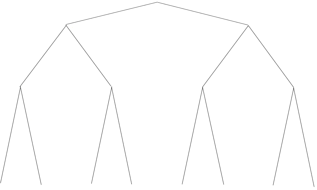
Figure 3: Regular tree, $\Gamma_{r}$, with the last generation formed by infinite edges.

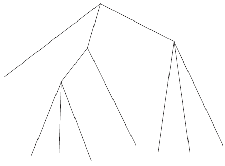
Figure 4: A more general tree, $\Gamma_{t}$, with vertices of degree greater or equal three.

In both cases, $\Gamma_{r}$ and $\Gamma_{t}$, we denote by $E_{v}$ the set of edges adjacent to the vertex $v$. For each vertex $v$ and $E_{v}$, we set, if the edge $e$ is of finite length,

$$i(v,e)=\left\{\begin{array}[]{lll}0,&v=\partial^{-}(e)\\ l_{e},&v=\partial^{+}(e)\end{array},\right.$$

otherwise $i(v,e)=0.$ The normal derivative of the restriction of $\psi$ on the edge $e\in E_{v}$ evaluated at the endpoints is

$$\dfrac{\partial\psi_{e}}{\partial n_{e}}(i(v,e))=\left\{\begin{array}[]{lll}-\psi^{\prime}_{e}(0_{+}),&i(v,e)=0\\ \psi^{\prime}_{e}({l_{e}}_{-}),&i(v,e)=l_{e}\\ \end{array}.\right.$$

Consider now the Laplacian with Kirchhoff coupling conditions at each vertex of the tree

$$\mathcal{D}(\Delta_{\Gamma})=\big{\{}\psi\in H^{2}(\Gamma):\ \psi_{e}(i(v,e))=\psi_{e^{\prime}}(i(v,e^{\prime})),e,e^{\prime}\in E_{v},\sum_{e\in E_{v}}\dfrac{\partial\psi_{e}}{\partial n_{e}}(i(v,e))=0,\ v\in V\big{\}},$$

where $\Gamma=\Gamma_{r}$ or $\Gamma=\Gamma_{t}$. In [20] (for $\Gamma_{r}$) and in [6] (for $\Gamma_{t}$), it was shown that the dispersive estimate (H.1) holds. Moreover, (H.2) is satisfied in both cases, since the form domain consists of $H^{1}(\Gamma)$ functions with continuity at the vertices.

3 Proofs of the main results

3.1 Proofs of results from Subsection 2.1

Proof of Proposition 2.4.

The fact that a.s. $(S_{\beta}(t,s)X_{s})_{t\geq s}$ has paths in $C([s,\infty),D(\Delta_{\Gamma}^{2}))$ and $|X(t)|_{L^{2}}=|X(s)|_{L^{2}},t\geq s$ follows directly from (2.7) and the properties of the deterministic Schrödinger group $(e^{it\Delta_{\Gamma}})_{t\in\mathbb{R}}$. To show that $S_{\beta}$ is the unique solution to (2.6), we rely on the following well known spectral representation of $f(-\Delta_{\Gamma})$ which holds for any continuous function $f:\mathbb{R}\rightarrow\mathbb{C}$:

$$f(-\Delta_{\Gamma})u_{0}=\lim\limits_{n}\lim\limits_{\varepsilon\to 0}\int_{-n}^{n}f(\lambda)[R_{\lambda+\mathrm{i}\varepsilon}-R_{\lambda-\mathrm{i}\varepsilon}]u_{0}\;d\lambda,\quad\forall u_{0}\in D(f(\Delta_{\Gamma})),$$ (3.1)

where $R(z):=(-\Delta_{\Gamma}-z)^{-1}$, for $z$ in the resolvent set of $-\Delta_{\Gamma}$. The limits are in $L^{2}(\Gamma)$, and their order cannot be reversed.

Let $X_{s}\in D(\Delta_{\Gamma}^{2})\ \mathbb{P}\mbox{-.a.s.}$ By (3.1), we have

$$S_{\beta}(t,s)X_{s}=\lim\limits_{n}\lim\limits_{\varepsilon\to 0}\int_{-n}^{n}{\mathrm{e}^{\mathrm{i}[\beta(t)-\beta(s)]\lambda}}[R_{\lambda+\mathrm{i}\varepsilon}-R_{\lambda-\mathrm{i}\varepsilon}]X_{s}\;d\lambda,$$ (3.2)

hence $(S_{\beta}(t,s)X_{s})_{t\geq s}$ is $(\mathcal{F}_{t})_{t\geq s}$-adapted. Using Itô formula for $\mathrm{e}^{\mathrm{i}[\beta(\cdot)-\beta(s)]\lambda}$ in (3.2), we easily arrive at

$$S_{\beta}(t,s)X_{s} =X_{s}+\mathrm{i}\lim\limits_{n}\lim\limits_{\varepsilon\to 0}\int_{-n}^{n}\int_{s}^{t}{\lambda}{\mathrm{e}^{\mathrm{i}[\beta(r)-\beta(s)]\lambda}}[R_{\lambda+\mathrm{i}\varepsilon}-R_{\lambda-\mathrm{i}\varepsilon}]X_{s}\;d\beta(r)\;d\lambda\qquad\qquad\qquad$$

$$\quad-{\frac{1}{2}}\lim\limits_{n}\lim\limits_{\varepsilon\to 0}\int_{-n}^{n}\int_{s}^{t}\lambda^{2}{\mathrm{e}^{\mathrm{i}[\beta(r)-\beta(s)]\lambda}}[R_{\lambda+\mathrm{i}\varepsilon}-R_{\lambda-\mathrm{i}\varepsilon}]X_{s}\;dr\;d\lambda.$$

By Fubini and dominated convergence theorems (classical and stochastic versions, see e.g. [14], [23]), but also (3.1), we get a.s.

$$S_{\beta}(t,s)X_{s} =X_{s}+\mathrm{i}\int_{s}^{t}\lim\limits_{n}\lim\limits_{\varepsilon\to 0}\int_{-n}^{n}{\lambda}{\mathrm{e}^{\mathrm{i}[\beta(r)-\beta(s)]\lambda}}[R_{\lambda+\mathrm{i}\varepsilon}-R_{\lambda-\mathrm{i}\varepsilon}]X_{s}\;d\lambda\;d\beta(r)$$

$$\ \ \qquad-{\frac{1}{2}}\int_{s}^{t}\lim\limits_{n}\lim\limits_{\varepsilon\to 0}\int_{-n}^{n}\lambda^{2}{\mathrm{e}^{\mathrm{i}[\beta(r)-\beta(s)]\lambda}}[R_{\lambda+\mathrm{i}\varepsilon}-R_{\lambda-\mathrm{i}\varepsilon}]X_{s}\;d\lambda\;dr$$

$$=X_{s}-{\frac{1}{2}}\int_{s}^{t}\Delta_{\Gamma}^{2}X(r)\;dr+\mathrm{i}\int_{s}^{t}\Delta_{\Gamma}X(r)\;d\beta(r)\;\quad\mbox{ for all }t\geq s.$$

Finally, if $(Z(t))_{t\geq 0}$ is another solution to (2.6), by similar spectral arguments and stochastic calculus as above, one can easily check that ${\mathrm{e}^{-\mathrm{i}[\beta(t)-\beta(s)]\Delta_{\Gamma}}}Z(t)=X_{s}\ \mathbb{P}\mbox{-a.s.}$ for all $t\geq 0$. But this clearly completes the proof since both $Y$ and $S_{\beta}(\cdot,s)$ have continuous paths, and by the group property of $({\mathrm{e}^{\mathrm{i}t\Delta_{\Gamma}}})_{t\in\mathbb{R}}$ we obtain

$$Z(t)={\mathrm{e}^{\mathrm{i}[\beta(t)-\beta(s)]\Delta_{\Gamma}}}X_{s}=S_{\beta}(t,s)\ \mathbb{P}\mbox{-.a.s.},\mbox{ for all }t\geq 0.\qed$$

Proof of Theorem 2.7.

Let us set for all $s$ and $t\in\mathbb{R}_{+}$,

$$S^{c}_{\beta}(t,s):=S_{\beta}(t,s)P_{c}\text{ and }S^{p}_{\beta}(t,s):=S_{\beta}(t,s)P_{p}.$$ (3.3)

Clearly, it is sufficient to prove the desired estimates for $S^{c}_{\beta}$ and $S^{p}_{\beta}$ separately. Concerning $S^{c}_{\beta}$, note first that from (H.1) and the fact that the deterministic group $(S(t))_{t\in\mathbb{R}}$ is an isometry on $L^{2}(\Gamma)$, by Riesz-Thorin interpolation theorem we get

$$\|S^{c}(t-s)X_{s}\|_{L^{p}(\Gamma)}\lesssim{|t-s|^{\frac{1}{p}-\frac{1}{2}}}\|X_{s}\|_{L^{p^{\prime}}(\Gamma)},\quad\text{for all }X_{s}\in L^{p^{\prime}}(\Gamma),$$

hence,

$$\|S^{c}_{\beta}(t,s)X_{s}\|_{L^{p}(\Gamma)}\lesssim{|\beta(t)-\beta(s)|^{\frac{1}{p}-\frac{1}{2}}}\|X_{s}\|_{L^{p^{\prime}}(\Gamma)},\quad\text{for all }X_{s}\in L^{p^{\prime}}(\Gamma)\ \mathbb{P}\mbox{-a.s.}$$

Then, the proofs of Propositions 3.7, 3.10 and 3.11 in [15] work without any change to get the estimates for $S^{c}_{\beta}$. In the case of $S^{p}_{\beta}$, for all $t\in\mathbb{R_{+}}$,

$$S^{p}_{\beta}(t)X_{s}=\sum_{j=1}^{|\sigma_{p}(-\Delta_{\Gamma})|}\mathrm{e}^{-\mathrm{i}\beta(t)\lambda_{j}}\langle X_{s},\varphi_{j}\rangle_{L^{2}(\Gamma)}\varphi_{j},$$

where $\lambda_{j}\in\mathbb{R}$ are the eigenvalues of $-\Delta_{\Gamma}$ and $\varphi_{j}$ the corresponding eigenfunctions, which by [21, Section 3], belong to $L^{\alpha}(\Gamma)$, for all $1\leq\alpha\leq\infty$. Let $(r,p)$ be an admissible pair. For every $\alpha\geq 1$, similarly to [18, Proof of Corollary 1] we get

$$\|S^{p}_{\beta}(t)X_{s}\|_{L^{p}(\Gamma)}\leq\Bigg{(}\sum_{j=1}^{|\sigma_{p}(-\Delta_{\Gamma})|}\|\varphi_{j}\|_{L^{\alpha^{\prime}}(\Gamma)}\|\varphi_{j}\|_{L^{p}(\Gamma)}\Bigg{)}\|X_{s}\|_{L^{\alpha}(\Gamma)},$$

$$\|S^{p}_{\beta}(\cdot,s)X_{s}\|_{L^{r}_{\omega}L^{r}_{[s,s+T]}L^{p}_{x}}\leq\Bigg{(}\sum_{j=1}^{|\sigma_{p}(-\Delta_{\Gamma})|}\|\varphi_{j}\|_{L^{\alpha^{\prime}}(\Gamma)}\|\varphi_{j}\|_{L^{p}(\Gamma)}\Bigg{)}T^{1/r}\|X_{s}\|_{L^{r}_{\omega}L^{\alpha}_{x}},$$ (3.4)

$$\Big{\|}\int_{s}^{\cdot}S^{p}_{\beta}(\cdot,\sigma)f(\sigma)\,d\sigma\Big{\|}_{L^{r}_{\omega}L^{r}_{[s,s+T]}L^{p}_{x}}\leq\Bigg{(}\sum_{j=1}^{|\sigma_{p}(-\Delta_{\Gamma})|}\|\varphi_{j}\|_{L^{\alpha^{\prime}}(\Gamma)}\|\varphi_{j}\|_{L^{p}(\Gamma)}\Bigg{)}T^{1/r}\|f\|_{L^{r}_{\omega}L^{1}_{[s,s+T]},L^{\alpha}_{x}},$$ (3.5)

which conclude the desired estimates. ∎

3.2 Proofs of results from Subsection 2.2

Proof of Theorem 2.8.

Denoting by $\mathcal{T}X^{R}$ the right hand side of (2.11), the latter becomes $X^{R}=\mathcal{T}X^{R}$. The proof which relies on the Strichartz type estimates obtained in Theorem 2.7, will be split in four steps.

Step 1. $\mathcal{T}$ is a contraction on the ”space-time-omega” balls:

$$E(T,a):=\{X\;\mathcal{F}_{t}-adapted:\;{\left|\kern-1.07639pt\left|\kern-1.07639pt\left|X\right|\kern-1.07639pt\right|\kern-1.07639pt\right|}:=|X|_{L^{r}_{\omega}L^{\infty}_{[0,T]}L_{x}^{2}}+|X|_{L^{r}_{\mathcal{P}}(\Omega\times[0,T];L^{p}_{x})}\leq a\}$$

for some convenient $a$ and $T$, where $T$ does not depend on the initial data so that this procedure can be iterated to obtain a global solution.

Step 2. The solution $X^{R}$ from Step 1 possesses extra integrability properties: for any $T>0$, $\rho\leq r$ and $(\rho,q)$ admissible,

$$X^{R}\in L^{\rho}_{[0,T]}L^{q}_{x}\;\;\;\mathbb{P}\mbox{-a.s.}$$

Step 3. $X^{R}$ has a version with trajectories in $C([0,T];L^{2}_{x})\;\;\;\mathbb{P}\mbox{-a.s.}$.

Step 4. For any $t>0$,

$$|X^{R}(t)|_{L^{2}_{x}}=|X_{0}|_{L^{2}_{x}}\;\;\;\mathbb{P}\mbox{-a.s.}$$

Proof of Step 1. Note that $E(T,a)$ is a complete metric space. First we find $T$ and $a$ such that $\mathcal{T}:E(T,a)\to E(T,a)$ is well-defined. To do this, for any $t\in[0,T]$, by the Strichartz type estimates from Theorem 2.7, we have

$$|\mathcal{T}X^{R}|_{L^{r}_{\omega}L^{\infty}_{[0,T]}L_{x}^{2}} \leq|X_{0}|_{L^{r}_{\omega}L_{x}^{2}}+\bigg{|}\int_{0}^{t}S_{\beta}(t,s)\theta_{R}(X^{R})(s)|X^{R}(s)|^{2\sigma}X^{R}(s)\;ds\bigg{|}_{L^{r}_{\omega}L^{\infty}_{[0,T]}L_{x}^{2}}$$

$$\leq|X_{0}|_{L^{r}_{\omega}L_{x}^{2}}+c_{r,p}\;T^{\overline{\beta}}\;\big{|}\theta_{R}(X^{R})|X^{R}|^{2\sigma+1}\;\big{|}_{L^{r}_{\omega}L^{r^{\prime}}_{[0,T]}L^{p^{\prime}}_{x}}$$

$$=|X_{0}|_{L^{r}_{\omega}L_{x}^{2}}+c_{r,p}\;T^{\overline{\beta}}\;\bigg{|}\bigg{[}\int_{0}^{T}\theta_{R}(X^{R})^{r^{\prime}}(t)\bigg{(}\int_{\Gamma}|X^{R}(t)|^{(2\sigma+1)p^{\prime}}\;dx\bigg{)}^{\frac{r^{\prime}}{p^{\prime}}}\;dt\bigg{]}^{1/r^{\prime}}\;\bigg{|}_{L^{r}_{\omega}}$$

Since $$p^{\prime}=\frac{2\sigma+2}{2\sigma+1}$$, the right hand side equals

$$=|X_{0}|_{L^{r}_{\omega}L_{x}^{2}}+c_{r,p}\;T^{\overline{\beta}}\;\bigg{|}\bigg{(}\int_{0}^{T}\theta_{R}(X^{R})^{r^{\prime}}(t)|X^{R}(t)|^{(2\sigma+1)r^{\prime}}_{L_{x}^{p}}\;dt\bigg{)}^{\frac{1}{r^{\prime}}}\;\bigg{|}_{L^{r}_{\omega}}$$

Since $$r\geq p=2\sigma+2$$, we can apply Hölder’s inequality to get

$$\leq|X_{0}|_{L^{r}_{\omega}L_{x}^{2}}+c_{r,p}\;T^{\overline{\beta}}\;\bigg{|}\bigg{(}\int_{0}^{T}[\theta_{R}(X^{R})(t)]^{r/(2\sigma+1)}|X^{R}(t)|^{r}_{L_{x}^{p}}\;dt\bigg{)}^{\frac{2\sigma+1}{r}}T^{\frac{r-r^{\prime}(2\sigma+1)}{rr^{\prime}}}\;\bigg{|}_{L^{r}_{\omega}}$$

Letting $$\widetilde{t}(\omega):=\inf\{s:\,|X^{R}(\omega)|_{L^{r}([0,s];L^{p}_{x})}\geq 2R\} \theta_{R}$$, from definition of in (2.9), we have

$$=|X_{0}|_{L^{r}_{\omega}L_{x}^{2}}+c_{r,p}\;T^{\tilde{\beta}}\;\bigg{|}\bigg{(}\int_{0}^{\widetilde{t}}[\theta_{R}(X^{R})(t)]^{r/(2\sigma+1)}|X^{R}(t)|^{r}_{L_{x}^{p}}\;dt\bigg{)}^{\frac{2\sigma+1}{r}}\;\bigg{|}_{L^{r}_{\omega}}$$

where $$\tilde{\beta}=\overline{\beta}+{\frac{r-r^{\prime}(2\sigma+1)}{rr^{\prime}}}>0$$. Furthermore,

$$\leq|X_{0}|_{L^{r}_{\omega}L_{x}^{2}}+c_{r,p}\;T^{\tilde{\beta}}\;\bigg{|}\bigg{(}\int_{0}^{\widetilde{t}}|X^{R}(t)|^{r}_{L_{x}^{p}}\;dt\bigg{)}^{\frac{2\sigma+1}{r}}\;\bigg{|}_{L^{r}_{\omega}}$$

$$\leq|X_{0}|_{L^{r}_{\omega}L_{x}^{2}}+c_{r,p}\;T^{\tilde{\beta}}\;(2R)^{2\sigma}\;\big{|}X^{R}\big{|}_{L^{r}_{\omega}L^{r}_{[0,T]}L_{x}^{p}}.$$

Similarly, using again the Strichartz type estimates,

$$|\mathcal{T}X^{R} |_{L^{r}_{\omega}L^{r}_{[0,T]}L_{x}^{p}}$$

$$\leq|S_{\beta}(t,0)X_{0}|_{L^{r}_{\omega}L^{r}_{[0,T]}L_{x}^{p}}+\bigg{|}\int_{0}^{t}S_{\beta}(t,s)\theta_{R}(X^{R})(s)|X^{R}(s)|^{2\sigma}X^{R}(s)\;ds\bigg{|}_{L^{r}_{\omega}L^{r}_{[0,T]}L_{x}^{p}}$$

$$\leq c_{r,p}\;T^{\beta/2}\;|X_{0}|_{L^{r}_{\omega}L_{x}^{2}}+c_{r,p}\;T^{\overline{\beta}}\;\big{|}\theta_{R}(X^{R})|X^{R}|^{2\sigma+1}\;\big{|}_{L^{r}_{\omega}L^{r^{\prime}}_{[0,T]}L_{x}^{p^{\prime}}}$$

$$\leq c_{r,p}\;T^{\beta/2}\;|X_{0}|_{L^{r}_{\omega}L_{x}^{2}}+c_{r,p}\;T^{\tilde{\beta}}\;(2R)^{2\sigma}\;\big{|}X^{R}\big{|}_{L^{r}_{\omega}L^{r}_{[0,T]}L_{x}^{p}}.$$ (3.6)

Hence,

$${\left|\kern-1.07639pt\left|\kern-1.07639pt\left|\mathcal{T}X^{R}\right|\kern-1.07639pt\right|\kern-1.07639pt\right|}\leq(1+c_{r,p}\;T^{\beta/2})\;|X_{0}|_{L^{r}_{\omega}L_{x}^{2}}+2\;c_{r,p}\;T^{\tilde{\beta}}\;(2R)^{2\sigma}\;\big{|}X^{R}\big{|}_{L^{r}_{\omega}L^{r}_{[0,T]}L_{x}^{p}}.$$

Letting $a:=2\;(1+c_{r,p}\;T^{\beta/2})\;|X_{0}|_{L^{r}_{\omega}L_{x}^{2}}$, there exists $T\leq 1$ which depends only on $R,r,p$ s.t. $c_{r,p}\;T^{\tilde{\beta}}\;(2R)^{2\sigma}<\dfrac{1}{4}$, so that ${\left|\kern-1.07639pt\left|\kern-1.07639pt\left|\mathcal{T}X^{R}\right|\kern-1.07639pt\right|\kern-1.07639pt\right|}\leq a$.

Now we prove that $\mathcal{T}$ is a contraction on $E(T,a)$. If $X$ and $Y$ $\in E(T,a)$, then by Strichartz estimates in Theorem 2.7,

$${\left|\kern-1.07639pt\left|\kern-1.07639pt\left|\mathcal{T}X-\mathcal{T}Y\right|\kern-1.07639pt\right|\kern-1.07639pt\right|} =\bigg{|}\int_{0}^{t}S_{\beta}(t,s)\bigg{[}\theta_{R}(X)(s)|X(s)|^{2\sigma}X(s)-\theta_{R}(Y)(s)|Y(s)|^{2\sigma}Y(s)\bigg{]}\;ds\bigg{|}_{L^{r}_{\omega}L^{\infty}_{[0,T]}L_{x}^{2}}$$

$$+\bigg{|}\int_{0}^{t}S_{\beta}(t,s)\bigg{[}\theta_{R}(X)(s)|X(s)|^{2\sigma}X(s)-\theta_{R}(Y)(s)|Y(s)|^{2\sigma}Y(s)\bigg{]}\;ds\bigg{|}_{L^{r}_{\omega}L^{r}_{[0,T]}L_{x}^{p}}$$

$$\leq c_{r,p}\;T^{\overline{\beta}}\;\big{|}\theta_{R}(X)|X|^{2\sigma}X-\theta_{R}(Y)|Y|^{2\sigma}Y\big{|}_{L^{r}_{\omega}L^{r^{\prime}}_{[0,T]}L_{x}^{p^{\prime}}}.$$

By [15, Proof of Theorem 4.1] we have that

$$\big{|}\theta_{R}(X)|X|^{2\sigma}X-\theta_{R}(Y)|Y|^{2\sigma}Y\big{|}_{L^{r}_{\omega}L^{r^{\prime}}_{[0,T]}L_{x}^{p^{\prime}}}\leq C\;T^{\gamma}\;|X-Y|_{L^{r}_{\omega}L^{r}_{[0,T]}L_{x}^{p}}$$

with $\gamma=1-\frac{2\sigma+2}{r}$, hence

$${\left|\kern-1.07639pt\left|\kern-1.07639pt\left|\mathcal{T}X-\mathcal{T}Y\right|\kern-1.07639pt\right|\kern-1.07639pt\right|}\leq c_{r,p}\;C\;T^{\tilde{\beta}+\gamma}\;{\left|\kern-1.07639pt\left|\kern-1.07639pt\left|X-Y\right|\kern-1.07639pt\right|\kern-1.07639pt\right|},$$

which means that if $T\leq T_{0}$ for some sufficiently small $T_{0}$, then $\mathcal{T}$ is a strict contraction on $E(T,a)$. Since $T_{0}$ does not depend on the initial data, we can iterate the construction and obtain a global solution for the truncated equation.

Proof of Step 2. If $\rho\leq r$ and $(\rho,q)$ is an admissible pair, by Theorem 2.7 (i) and (ii.2) we get

$$|X^{R}|_{L^{\rho}_{\omega}L^{\rho}_{[0,T]}L_{x}^{q}} \leq c_{\rho,q}T^{\beta/2}|X_{0}|_{L^{\rho}_{\omega}L^{2}_{x}}+\tilde{c}_{\rho,q}T^{\overline{\beta}}\big{|}\theta_{R}(X^{R})|X^{R}|^{2\sigma+1}\;\big{|}_{L^{\rho}_{\omega}L^{r^{\prime}}_{[0,T]}L^{p^{\prime}}_{x}}$$

$$\leq c_{\rho,q}T^{\beta/2}|X_{0}|_{L^{\rho}_{\omega}L^{2}_{x}}+\tilde{c}_{\rho,q}T^{\overline{\beta}}\big{|}\theta_{R}(X^{R})|X^{R}|^{2\sigma+1}\;\big{|}_{L^{r}_{\omega}L^{r^{\prime}}_{[0,T]}L_{x}^{p^{\prime}}}$$

$$\leq c_{\rho,q}T^{\beta/2}|X_{0}|_{L^{\rho}_{\omega}L^{2}_{x}}+\tilde{c}_{\rho,q}T^{\overline{\beta}}(2R)^{2\sigma}\;\big{|}X^{R}\big{|}_{L^{r}_{\omega}L^{r}_{[0,T]}L_{x}^{p}}<\infty.$$

Proof of Step 3. We claim that

$$X^{R}(t)=S_{\beta}(t,0)X_{0}+\mathrm{i}S_{\beta}(t,0)\int_{0}^{t}S_{\beta}(0,s)\theta_{R}(X^{R})|X^{R}|^{2\sigma}X^{R}(s)\,ds.$$ (3.7)

Note that since $S_{\beta}(t,0)\in\mathcal{L}(L^{2}_{x},L^{2}_{x})$, it is sufficient to check the Bochner integrability of the integrand. Indeed,

$$\int_{0}^{T}\big{|}S_{\beta}(0,s)\theta_{R}(X^{R})|X^{R}|^{2\sigma}X^{R}(s)\big{|}_{L^{2}_{x}}\,ds =\int_{0}^{T}\big{|}\theta_{R}(X^{R})|X^{R}|^{2\sigma}X^{R}(s)\big{|}_{L^{2}_{x}}\,ds$$

$$\leq\int_{0}^{T}\big{|}|X^{R}|^{2\sigma+1}\big{|}_{L^{2}_{x}}\,ds=\int_{0}^{T}\Big{[}\int_{\Gamma}|X^{r}|^{2(2\sigma+1)}\,dx\Big{]}^{1/2}\,ds$$

$$=|X^{R}|^{2\sigma+1}_{L^{2\sigma+1}_{[0,T]}L^{2(2\sigma+1)}_{x}}$$

Since $\sigma<2$, the exponent pair $(2\sigma+1,2(2\sigma+1))$ is admissible and hence, by the additional integrability obtained at Step 2,

$$|X^{R}|_{L^{2\sigma+1}_{\omega}L^{2\sigma+1}_{[0,T]}L^{2(2\sigma+1)}_{x}}<\infty\text{ and hence }|X^{R}|_{L^{2\sigma+1}_{[0,T]}L^{2(2\sigma+1)}_{x}}<\infty\;\;\;\mathbb{P}\mbox{-a.s.}$$

So,

$$\int_{0}^{T}\big{|}S_{\beta}(0,s)\theta_{R}(X^{R})|X^{R}|^{2\sigma}X^{R}(s)\big{|}_{L^{2}_{x}}\,ds\leq|X^{R}|^{2\sigma+1}_{L^{2\sigma+1}_{[0,T]}L^{2(2\sigma+1)}_{x}}<\infty.$$ (3.8)

Let now $Y(t):=S_{\beta}(0,t)X^{R}(t)$. Then, by (3.7)

$$Y(t)=X_{0}+\mathrm{i}\int_{0}^{t}S_{\beta}(0,s)\theta_{R}(X^{R})|X^{R}|^{2\sigma}X^{R}(s)\,ds\;\;\;\mathbb{P}\mbox{-a.s.}\,for\ all\ t\in[0,T].$$

Since the integrand belongs to $L^{1}([0,T];L^{2}_{x})$, it follows that $(Y(t))_{t\in[0,T]}$ has a version with absolutely continuous trajectories in $[0,T]$ with values in $L^{2}_{x}$, which we again denote by $Y$. We show now that $(S_{\beta}(t,0)Y(t))_{t\in[0,T]}$, which is a version of $(X^{R}(t))_{t\in[0,T]}$, has continuous trajectories with values in $L^{2}_{x}$. We have that

$$\big{|}S_{\beta}(t,0)Y(t) -S_{\beta}(s,0)Y(s)\big{|}_{L^{2}_{x}}$$

$$\leq\big{|}S_{\beta}(t,0)Y(t)-S_{\beta}(s,0)Y(t)\big{|}_{L^{2}_{x}}+\big{|}S_{\beta}(s,0)Y(t)-S_{\beta}(s,0)Y(s)\big{|}_{L^{2}_{x}}$$

$$=\big{|}[S_{\beta}(t,0)-S_{\beta}(s,0)]Y(t)\big{|}_{L^{2}_{x}}+\big{|}Y(t)-Y(s)\big{|}_{L^{2}_{x}}.$$

So, by the continuity of the group and the fact that $(Y(t))_{t\in[0,T]}$ is with absolutely continuous trajectories, we get the desired result.

Proof of Step 4. Note that since $S(t)$ is an isometry on $L^{2}_{x}$, the conservation of the $L^{2}_{x}$–norm of $X^{R}$ is equivalent with the $L^{2}_{x}$-norm conservation of $Y(t)$. Clearly, $\phi:[0,T]\to\mathbb{R}_{+}$ defined as $\phi(t):=|Y(t)|_{L^{2}_{x}}$ is absolutely continuous, hence it is sufficient to show that $\phi^{\prime}=0\,\,\lambda-\mbox{a.e.}$ This holds true because

$$\frac{d}{dt}|Y(t)|_{L^{2}_{x}}^{2} =2\Re\{\langle\frac{d}{dt}Y(t),Y(t)\rangle_{L^{2}_{x}}\}$$

$$=2\Re\{\mathrm{i}\langle S_{\beta}(0,t)\theta_{R}(X^{R})|X^{R}|^{2\sigma}X^{R}(t),S_{\beta}(0,t)X^{R}(t)\rangle_{L^{2}_{x}}\}$$

$$=2\Re\{\mathrm{i}\langle\theta_{R}(X^{R})|X^{R}|^{2\sigma}X^{R}(t),X^{R}(t)\rangle_{L^{2}_{x}}\}=0.$$

Hence, $\phi(t)=\phi(0)$ for all $t\in[0,T],$ which completes our proof. ∎

3.3 Proofs of results from Subsection 2.3

Proof of Theorem 2.11.

Well-posedness in $\bm{C([0,T],L^{2}(\Gamma))}$. Consider the complete metric function space

$$E(T,a)=\{u\in C([0,T],L^{2}(\Gamma)):\|u\|_{C([0,T],L^{2}(\Gamma))}:=\sup_{t\in[0,T]}\|u(t)\|_{L^{2}(\Gamma)}\leq a\},$$

where $T,a\in\mathbb{R}_{+}$ will be chosen later. Denote by $\uptau(u_{n})(t)$ the right hand side of (2.14).

First of all, note that if $u_{n}\in C([0,T];L^{2}(\Gamma))$ then $F(u_{n})\in L^{\infty}([0,T];L^{2}(\Gamma))$. Hence, we can use the same argument as in Step 3 of the proof of Theorem 2.8 to deduce that $\uptau(u_{n})\in C([0,T];L^{2}(\Gamma))$. Moreover,

$$\|\uptau(u_{n})\|_{C([0,T],L^{2}(\Gamma))}\leq\|u_{0}\|_{L^{2}(\Gamma)}+(2R^{\sigma})\,T\,\|u_{n}\|_{C([0,T],L^{2}(\Gamma))}.$$

Hence, taking for instance $a=2\|u_{0}\|_{L^{2}(\Gamma)}$ and $T\leq\dfrac{1}{2(2R)^{\sigma}}$, $\uptau:E(T,a)\to E(T,a)$ is well-defined.

Let now $u,v\in E(T,a)$, with $T$ and $a$ as before. Then,

$$\|\uptau(u)(t)-\uptau(v)(t)\|_{L^{2}(\Gamma)} \leq\int_{0}^{t}\|F(u)-F(v)\|_{L^{2}(\Gamma)}\,ds\leq C(R,\sigma)\int_{0}^{t}\|u(s)-v(s)\|_{L^{2}(\Gamma})\,ds,$$

Therefore,

$$\|\uptau(u)-\uptau(v)\|_{C([0,T],L^{2}(\Gamma))}\leq C(R,\sigma)\,T\,\|u-v\|_{C([0,T],L^{2}(\Gamma))}.$$

Taking now $T\leq\min\bigg{(}\dfrac{1}{2(2R)^{\sigma}},\dfrac{1}{C(R,\sigma)}\bigg{)}$, we deduce that $\uptau:E(T,a)\to E(T,a)$ is a strict contraction, hence, there exists a unique solution $u_{n}\in C([0,T],L^{2}(\Gamma))$ to (2.14). Since $T$ does depend only on the nonlinearity $F$, we can reiterate to get a global solution.

Well-posedness in $\bm{C([0,T],D(\mathcal{E}))}$. By the properties of $F$,

$$\|F(u_{n})\|_{D(\mathcal{E})}\leq C(R,\sigma)\|u_{n}\|_{D(\mathcal{E})}.$$ (3.9)

Since $u_{0}\in D(\mathcal{E})\subset L^{2}(\Gamma)$, by the first part we have a unique solution $u_{n}\in C([0,T],L^{2}(\Gamma))$.

We show that $u_{n}$ belongs to $C([0,T],D(\mathcal{E}))$. To this end, note that $u_{n}$ is the limit in $C([0,T];L^{2}(\Gamma))$ of the sequence $(u_{n}^{k})_{k}$ constructed as follows:

$$u_{n}^{0}=u_{0}$$

$$u_{n}^{k+1}(\cdot)=\uptau(u_{n}^{k})(\cdot)=S_{n}(\cdot,0))u^{0}+\mathrm{i}\int_{0}^{\cdot}S_{n}(\cdot,s)F(u_{n}^{k})(s)\,ds,\quad\text{for all }k\geq 0.$$

So, using (3.9) we get

$$\|u_{n}^{k+1}(t)\|_{D(\mathcal{E})} \leq\|u^{0}\|_{D(\mathcal{E})}+\int_{0}^{t}\|F(u_{n}^{k}(s))\|_{D(\mathcal{E})}\,ds\leq\|u_{n}^{0}\|_{D(\mathcal{E})}+C(R,\sigma)\int_{0}^{t}\|u_{n}^{k}(s)\|_{D(\mathcal{E})}\,ds.$$

Hence, if $v^{k}(t):=\|u_{n}^{k}(t)\|_{D(\mathcal{E})}$, we have for all $t\geq 0$ and $k\geq 0$

$$v^{k+1}(t)\leq v^{0}+C\int_{0}^{t}v^{k}(s)\,ds.$$

Hence, by [15, Lemma 3.2 (i)],

$$\|u_{n}^{k}(t)\|_{D(\mathcal{E})}\leq\|u_{0}\|_{D(\mathcal{E})}\mathrm{e}^{C(R,\sigma)T},\quad\forall t\leq T.$$

Thus, for each fixed $t$, $(u_{n}^{k}(t))_{k}$ is a bounded sequence in the Hilbert space $D(\mathcal{E})$, hence there exists a subsequence $(u_{n}^{k_{l}})_{l}$ which is weakly convergent to some limit in $D(\mathcal{E})$. Since

$$u_{n}^{k}(t)\underset{k\to\infty}{\longrightarrow}u_{n}(t)\in L^{2}(\Gamma),$$

we get that $u_{n}(t)\in D(\mathcal{E})$ for all $t\in[0,T]$. Since the norm on $D(\mathcal{E})$ is lower semi-continuous w.r.t. the weak topology, we also get

$$\|u_{n}(t)\|_{D(\mathcal{E})}\leq\|u_{0}\|_{D(\mathcal{E})}\mathrm{e}^{C(R,\sigma)T},\quad\forall t\leq T.$$ (3.10)

To show that $u_{n}\in C([0,T],D(\mathcal{E}))$, note first that $(S(t))_{t\in\mathbb{R}}$ is a continuous group on $D(\mathcal{E})$, since for all $u_{0}\in D(\mathcal{E})$ and $t_{k}\to 0$, by the spectral representation and the spectral measure property (3.16),

$$\|S(t_{k})u_{0}-S(t)u_{0}\|^{2}_{D(\mathcal{E})}=\int_{\sigma(-\Delta_{\Gamma})}(\lambda+M)|1-cos[(t_{k}-t)\lambda]|\,d\mu_{u_{0},u_{0}}(\lambda)$$

converges to $0$ when $k\to\infty$ by dominated convergence, since $\lambda+M\in L^{1}(\sigma(-\Delta_{\Gamma}),d\mu_{u_{0},u_{0}})$ because $u_{0}\in D(\mathcal{E})$.

Then, the desired continuity follows by dominated convergence theorem and (3.9), since

$$\|S(t_{n}-s)F(u(s))\|_{D(\mathcal{E})} \leq\|F(u(s))\|_{D(\mathcal{E})}\leq C(R,\sigma)\|u_{0}\|_{D(\mathcal{E})}\mathrm{e}^{C(R,\sigma)T}$$

$$\leq C(R,\sigma)\|u_{0}\|_{D(\mathcal{E})}\mathrm{e}^{C(R,\sigma)T}\in L^{1}([0,T]).\qed$$

Proof of Theorem 2.13.

Denote by $\beta_{\varepsilon}(\cdot):=\int_{0}^{\cdot}\frac{1}{\varepsilon}m\big{(}\frac{s}{\varepsilon^{2}}\big{)}\,ds$, with the process $m$ as in (H.0). Since by hypothesis, $\beta_{\varepsilon}$ converges to $\beta$ converges in distribution on $C([0,T];\mathbb{R})$ for all $T>0$ it is sufficient to show that the mapping

$$C([0,T];\mathbb{R})\ni n\longmapsto u_{n}\in C([0,T];D(\mathcal{E}))$$

is continuous, where $u_{n}$ is the solution of (2.14). First of all, since $\|\cdot\|_{D(\mathcal{E})}$ is equivalent with $\|\cdot\|_{H^{1}}$ (2.3), one can easily check that

$$\|F(v)-F(w)\|_{D(\mathcal{E})}\leq C(R,\sigma)(1+\|w\|_{D(\mathcal{E})})\|v-w\|_{D(\mathcal{E})},$$

for all $v$ and $w$ in $D(\mathcal{E})$. Consequently, if $n_{k}\underset{k\to\infty}{\longrightarrow}n\in C([0,T];\mathbb{R})$, using also the fact that $S(t)$ is an isometry on $D(\mathcal{E})$,

$$\|u_{n_{k}}(t)-u_{n}(t)\|_{D(\mathcal{E})} \leq\int_{0}^{t}\Big{\|}[S_{n_{k}}(t,s)-S_{n}(t,s)]F(u_{n})(s)\Big{\|}_{D(\mathcal{E})}\,ds$$

$$\quad+\int_{0}^{t}\Big{\|}S_{n_{k}}(t,s)[F(u_{n_{k}})(s)-F(u_{n})(s)]\Big{\|}_{D(\mathcal{E})}\,ds$$

$$\leq\int_{0}^{T}\Big{\|}[S_{n_{k}}(\cdot,s)-S_{n}(\cdot,s)]F(u_{n})(s)\Big{\|}_{C([0,T];D(\mathcal{E}))}\,ds$$

$$\quad+C(R,\sigma)[1+\|u_{n}\|_{C([0,T];D(\mathcal{E}))}]\int_{0}^{t}\|u_{n_{k}}(s)-u_{n}(s)\|_{D(\mathcal{E})}\,ds.$$

If we denote the first term in r.h.s. of the last inequality by $a_{k}$, we get by Grönwall lemma

$$\|u_{n_{k}}-u_{n}\|_{C([0,T];D(\mathcal{E}))}\leq a_{k}\mathrm{e}^{C(R,\sigma)[1+\|u_{n}\|_{C([0,T];D(\mathcal{E}))}]T}.$$

But $a_{k}\mathop{\longrightarrow}\limits_{k\to\infty}0$ by dominated convergence, since

$$\Big{\|}[S_{n_{k}}(\cdot,s)-S_{n}(\cdot,s)]F(u_{n})(s)\Big{\|}_{C([0,T];D(\mathcal{E}))}\leq 2\|F(u_{n})(s)\|_{D(\mathcal{E})}\leq 2|f|_{\infty}\|u_{n}\|_{C([0,T];D(\mathcal{E}))}$$

and

$$\Big{\|}[S_{n_{k}}(\cdot,s) -S_{n}(\cdot,s)]F(u_{n})(s)\Big{\|}^{2}_{C([0,T];D(\mathcal{E}))}$$

$$\leq 2\int_{\sigma(-\Delta_{\Gamma})}(\lambda+M)[2\wedge|\lambda||n_{k}(\cdot)-n_{k}(s)-(n(\cdot)-n(s))|]\,d\mu_{F(u_{n}),F(u_{n})}(\lambda)$$

which converges to $0$ for all $s\in[0,T]$, again by dominated convergence since $F(u_{n})\in D(\mathcal{E})$. ∎

3.4 Proofs of results from Subsection 2.4

Proof of Proposition 2.16.

We need the following claim whose proof is postponed right after the proof of Proposition 2.16.

Claim 1.

If $u_{0}\in D(\mathcal{E}_{\star})$, then $\lim_{\varepsilon\to 0}\mathrm{e}^{-(\mathrm{i}t+\varepsilon)H_{\star}}u_{0}=\mathrm{e}^{-\mathrm{i}tH_{\star}}u_{0}\ \text{ in }H^{1}(\Gamma).$

As in the proof of Proposition 2.14, let $n_{+}(AB^{{\dagger}})$ be the number of (negative) eigenvalues $(\lambda_{l})_{l}$ of $H_{\star}$ and denote by $(\varphi_{l})_{l}$ the corresponding eigenfunctions. By [18, Proposition 3.2] and e.g. [26, Theorem VII.11], the continuous spectrum of $H_{\star}$ is $[0,\infty)$. Consequently, we have the following representation:

$$\mathrm{e}^{-(\mathrm{i}t+\varepsilon)H_{\star}}u_{0}(x)=\frac{1}{2\pi\mathrm{i}}\lim_{\delta\to 0}\int_{0}^{\infty}\mathrm{e}^{-(\mathrm{i}t+\varepsilon)\lambda}[R_{\lambda+\mathrm{i}\delta}-R_{\lambda-\mathrm{i}\delta}]u_{0}(x)\,d\lambda+\sum_{l=1}^{n_{+}(AB^{{\dagger}})}\langle u_{0},\varphi_{l}\rangle\mathrm{e}^{-(\mathrm{i}t+\varepsilon)\lambda_{l}}\varphi_{l}$$

and the limit is in $L^{2}(\Gamma_{\star})$, where $R_{z}:=(H_{\star}-z)^{-1}$. Taking into account the explicit kernel obtained in [21, Lemma 4.2], we arrive at:

$$\mathrm{e}^{-(\mathrm{i}t+\varepsilon)H_{\star}}u_{0}(x_{i})$$

$$=\dfrac{1}{2\pi\mathrm{i}}\lim_{\delta\to 0}\int_{0}^{\infty}\mathrm{e}^{-(\mathrm{i}t+\varepsilon)\lambda}\Big{\{}\sum_{j=1}^{n}\int_{I_{j}}[r(\sqrt{\lambda+\mathrm{i}\delta};x_{i},y_{j})-r(\sqrt{\lambda-\mathrm{i}\delta};x_{i},y_{j})]u_{0}(y_{j})\,dy_{j}\Big{\}}\,d\lambda$$

$$+\sum_{l=1}^{n_{+}(AB^{{\dagger}})}\langle u_{0},\varphi_{l}\rangle\mathrm{e}^{-(\mathrm{i}t+\varepsilon)\lambda_{l}}\varphi_{l}(x),$$

with the matrix kernel $r(z;x;y)$ s.t. $r(z;x_{i},y_{j})=\dfrac{\mathrm{i}}{2z}\mathrm{e}^{\mathrm{i}z|x_{i}-y_{j}|}\delta_{ij}+\dfrac{\mathrm{i}}{2z}\mathrm{e}^{\mathrm{i}zx_{i}}[G(z;A,B)]_{i,j}\mathrm{e}^{\mathrm{i}zy_{j}}$,

where $z^{2}\in\mathbb{C}\setminus\sigma(H_{\star})$, $x_{i}$ and $y_{j}$ belong to the edges $I_{i}$ and $I_{j}$ respectively, $i,j=\overline{1,n}$ and the matrix $G$ is given by $G(z;A,B)=-(A+\mathrm{i}zB)^{-1}(A-\mathrm{i}zB)$.

Claim 2.

If $u_{0}\in D(\mathcal{E}_{\star})$, then for all $1\leq i\leq n$,

$$\partial_{x_{i}}(\mathrm{e}^{-(\mathrm{i}t+\varepsilon)H_{\star}}u_{0}(x_{i}))$$

$$=\dfrac{1}{2\pi\mathrm{i}}\lim_{\delta\to 0}\partial_{x_{i}}\int_{0}^{\infty}\mathrm{e^{-(\mathrm{i}t+\varepsilon)\lambda}}\Big{\{}\sum_{j=1}^{n}\int_{I_{j}}[r(\sqrt{\lambda+\mathrm{i}\delta};x_{i},y_{j})-r(\sqrt{\lambda-\mathrm{i}\delta};x_{i},y_{j})]u_{0}(y_{j})\,dy_{j}\Big{\}}\,d\lambda$$

$$+\sum_{l=1}^{n_{+}(AB^{{\dagger}}}\langle u_{0},\varphi_{l}\rangle\mathrm{e}^{-(\mathrm{i}t+\varepsilon)\lambda_{l}}\varphi^{\prime}_{l}(x_{i}).$$

Let us now deal with the first term in the above r.h.s. and notice that

$$\partial_{x_{i}} \int_{0}^{\infty}\mathrm{e^{-(\mathrm{i}t+\varepsilon)\lambda}}\Big{\{}\sum_{j=1}^{n}\int_{I_{j}}[r(\sqrt{\lambda+\mathrm{i}\lambda};x_{i},y_{j})-r(\sqrt{\lambda-\mathrm{i}\delta};x_{i},y_{j})]u_{0}(y_{j})\,dy_{j}\Big{\}}\,d\lambda$$

$$=\int_{0}^{\infty}\mathrm{e^{-(\mathrm{i}t+\varepsilon)\lambda}}\Big{\{}\sum_{j=1}^{n}\int_{I_{j}}\partial_{x_{i}}[r(\sqrt{\lambda+\mathrm{i}\delta};x_{i},y_{j})-r(\sqrt{\lambda-\mathrm{i}\delta};x_{i},y_{j})]u_{0}(y_{j})\,dy_{j}\Big{\}}\,d\lambda$$

$$=:\int_{0}^{\infty}\mathrm{e^{-(\mathrm{i}t+\varepsilon)\lambda}}\sum_{j=1}^{n}[I_{(j)}(\sqrt{\lambda+\mathrm{i}\delta};x_{i})-I_{(j)}(\sqrt{\lambda-\mathrm{i}\delta};x_{i})]\,d\lambda.$$ (3.11)

We treat now the integrands $I_{(j)}(\sqrt{\lambda\pm\mathrm{i}\delta};x_{i})$:

$$I_{(j)}(\sqrt{\lambda\pm\mathrm{i}\delta};x_{i})=\int_{I_{j}}\partial_{x}r(\sqrt{\lambda\pm\mathrm{i}\delta};x_{i},y_{j})u_{0}(y_{j})\,dy_{j}$$

$$=\int_{I_{j}}\partial_{x_{i}}\Bigg{[}\frac{\mathrm{i}}{2\sqrt{\lambda\pm\mathrm{i}\delta}}\mathrm{e}^{\mathrm{i}\sqrt{\lambda\pm\mathrm{i}\delta}|x_{i}-y_{j}|}\delta_{ij}+\dfrac{\mathrm{i}}{2\sqrt{\lambda\pm\mathrm{i}\delta}}\mathrm{e}^{\mathrm{i}\sqrt{\lambda\pm\mathrm{i}\delta}x_{i}}[G(\sqrt{\lambda\pm\mathrm{i}\delta};A,B)]_{i,j}\mathrm{e}^{\mathrm{i}\sqrt{\lambda\pm\mathrm{i}\delta}y_{j}}\Bigg{]}u_{0}(y_{j})\,dy_{j}$$

$$=\int_{I_{j}}\Bigg{[}\frac{\mathrm{i}}{2\sqrt{\lambda\pm\mathrm{i}\delta}}\mathrm{i}\sqrt{\lambda\pm\mathrm{i}\delta}\operatorname{sign}(x_{i}-y_{j})\mathrm{e}^{\mathrm{i}\sqrt{\lambda\pm\mathrm{i}\delta}|x_{i}-y_{j}|}\delta_{ij}$$

$$\qquad+\dfrac{\mathrm{i}}{2\sqrt{\lambda\pm\mathrm{i}\delta}}\mathrm{i}\sqrt{\lambda\pm\mathrm{i}\delta}\mathrm{e}^{\mathrm{i}\sqrt{\lambda\pm\mathrm{i}\delta}x_{i}}[G(\sqrt{\lambda\pm\mathrm{i}\delta};A,B)]_{i,j}\mathrm{e}^{\mathrm{i}\sqrt{\lambda\pm\mathrm{i}\delta}y_{j}}\Bigg{]}u_{0}(y_{j})\,dy_{j}$$

$$=\int_{I_{j}}\partial_{y_{j}}\Bigg{[}\frac{-\mathrm{i}}{2\sqrt{\lambda\pm\mathrm{i}\delta}}\mathrm{e}^{\mathrm{i}\sqrt{\lambda\pm\mathrm{i}\delta}|x_{i}-y_{j}|}\delta_{ij}+\dfrac{\mathrm{i}}{2\sqrt{\lambda\pm\mathrm{i}\delta}}\mathrm{e}^{\mathrm{i}\sqrt{\lambda\pm\mathrm{i}\delta}x_{i}}[G(\sqrt{\lambda\pm\mathrm{i}\delta};A,B)]_{i,j}\mathrm{e}^{\mathrm{i}\sqrt{\lambda\pm\mathrm{i}\delta}y_{j}}\Bigg{]}u_{0}(y_{j})\,dy_{j}.$$

Integrating by parts, we continue with

$$=\dfrac{\mathrm{i}}{2\sqrt{\lambda\pm\mathrm{i}\delta}}\mathrm{e}^{\mathrm{i}\sqrt{\lambda\pm\mathrm{i}\delta}x_{i}}\Big{[}\delta_{ij}-[G(\sqrt{\lambda\pm\mathrm{i}\delta};A,B)]_{i,j}\Big{]}u_{0,j}(0)$$

$$-\int_{I_{j}}\Bigg{[}\frac{-\mathrm{i}}{2\sqrt{\lambda\pm\mathrm{i}\delta}}\mathrm{e}^{\mathrm{i}\sqrt{\lambda\pm\mathrm{i}\delta}|x_{i}-y_{j}|}\delta_{ij}+\dfrac{\mathrm{i}}{2\sqrt{\lambda\pm\mathrm{i}\delta}}\mathrm{e}^{\mathrm{i}\sqrt{\lambda\pm\mathrm{i}\delta}x_{i}}[G(\sqrt{\lambda\pm\mathrm{i}\delta};A,B)]_{i,j}\mathrm{e}^{\mathrm{i}\sqrt{\lambda\pm\mathrm{i}\delta}y_{j}}\Bigg{]}u^{\prime}_{0,j}(y_{j})\,dy_{j}$$

Hence,

$$I_{(j)}(\sqrt{\lambda+\mathrm{i}\delta}; x_{i})-I_{(j)}(\sqrt{\lambda-\mathrm{i}\delta};x_{i})=\dfrac{\mathrm{i}}{2\sqrt{\lambda+\mathrm{i}\delta}}\mathrm{e}^{\mathrm{i}\sqrt{\lambda+\mathrm{i}\delta}x_{i}}\Big{[}\delta_{ij}-[G(\sqrt{\lambda+\mathrm{i}\delta};A,B)]_{i,j}\Big{]}u_{0,j}(0)$$

$$\quad\qquad\qquad\qquad\qquad-\dfrac{\mathrm{i}}{2\sqrt{\lambda-\mathrm{i}\delta}}\mathrm{e}^{\mathrm{i}\sqrt{\lambda-\mathrm{i}\delta}x_{i}}\Big{[}\delta_{ij}-[G(\sqrt{\lambda-\mathrm{i}\delta};A,B)]_{i,j}\Big{]}u_{0,j}(0)$$

$$-\int_{I_{j}}[r(\sqrt{\lambda+\mathrm{i}\delta};x_{i},y_{j})-r(\sqrt{\lambda-\mathrm{i}\delta};x_{i},y_{j})]u^{\prime}_{0,j}(y_{j})\,dy_{j}$$

$$+2\int_{I_{j}}\frac{\mathrm{i}}{2\sqrt{\lambda+\mathrm{i}\delta}}\mathrm{e}^{\mathrm{i}\sqrt{\lambda+\mathrm{i}\delta}|x_{i}-y_{j}|}\delta_{ij}u^{\prime}_{0,j}(y_{j})-\dfrac{\mathrm{i}}{2\sqrt{\lambda-\mathrm{i}\delta}}\mathrm{e}^{\mathrm{i}\sqrt{\lambda-\mathrm{i}\delta}|x_{i}-y_{j}|}\delta_{ij}u^{\prime}_{0,j}(y_{j})\,dy_{j}.$$

Substituting this back in (3.4), we get that

$$\partial_{x_{i}}(\mathrm{e}^{-(\mathrm{i}t+\varepsilon)H_{\star}}u_{0}(x_{i}))=\dfrac{1}{2\pi\mathrm{i}}\lim_{\delta\to 0}\int_{0}^{\infty}\mathrm{e}^{-(\mathrm{i}t+\varepsilon)\lambda}\sum_{j=1}^{n}\Big{\{}\dfrac{\mathrm{i}}{2\sqrt{\lambda+\mathrm{i}\delta}}\mathrm{e}^{\mathrm{i}\sqrt{\lambda+\mathrm{i}\delta}x_{i}}[\delta_{ij}-[G(\sqrt{\lambda+\mathrm{i}\delta};A,B)]_{i,j}]$$

$$\qquad\qquad\qquad\qquad\qquad-\dfrac{\mathrm{i}}{2\sqrt{\lambda-\mathrm{i}\delta}}\mathrm{e}^{\mathrm{i}\sqrt{\lambda-\mathrm{i}\delta}x_{i}}[\delta_{ij}-[G(\sqrt{\lambda-\mathrm{i}\delta};A,B)]_{i,j}]\Big{\}}u_{0,j}(0)\,d\lambda$$

$$-\dfrac{1}{2\pi\mathrm{i}}\lim_{\delta\to 0}\int_{0}^{\infty}\mathrm{e}^{-(\mathrm{i}t+\varepsilon)\lambda}\sum_{j=1}^{n}\int_{I_{j}}[r(\sqrt{\lambda+\mathrm{i}\delta};x_{i},y_{j})-r(\sqrt{\lambda-\mathrm{i}\delta};x_{i},y_{j})]u^{\prime}_{0,j}(y_{j})\,dy_{j}\,d\lambda$$

$$+\dfrac{1}{2\pi\mathrm{i}}\lim_{\delta\to 0}\int_{0}^{\infty}2\mathrm{e}^{-(\mathrm{i}t+\varepsilon)\lambda}\int_{I_{i}}\frac{\mathrm{i}}{2\sqrt{\lambda+\mathrm{i}\delta}}\mathrm{e}^{\mathrm{i}\sqrt{\lambda+\mathrm{i}\delta}|x_{i}-y_{i}|}u^{\prime}_{0,i}(y_{i})-\dfrac{\mathrm{i}}{2\sqrt{\lambda-\mathrm{i}\delta}}\mathrm{e}^{\mathrm{i}\sqrt{\lambda-\mathrm{i}\delta}|x_{i}-y_{i}|}u^{\prime}_{0,i}(y_{i})\,dy_{i}\,d\lambda$$

$$=:J_{1}+J_{2}+J_{3}$$ (3.12)

By the spectral theorem, $J_{2}=\mathrm{e}^{-(\mathrm{i}t+\varepsilon)H_{\star}}P_{c}u^{\prime}_{0}(x_{i})$. By (2.16),

$$J_{3}=\dfrac{1}{2\pi\mathrm{i}}\lim_{\delta\to 0}\int_{0}^{\infty}2\mathrm{e}^{-(\mathrm{i}t+\varepsilon)\lambda}\int_{\mathbb{R}}\frac{\mathrm{i}}{2\sqrt{\lambda+\mathrm{i}\delta}}\mathrm{e}^{\mathrm{i}\sqrt{\lambda+\mathrm{i}\delta}|x_{i}-y_{i}|}\widetilde{u^{\prime}}_{0,i}(y_{i})-\dfrac{\mathrm{i}}{2\sqrt{\lambda-\mathrm{i}\delta}}\mathrm{e}^{\mathrm{i}\sqrt{\lambda-\mathrm{i}\delta}|x_{i}-y_{i}|}\widetilde{u^{\prime}}_{0,i}(y_{i})\,dy_{i}\,d\lambda.$$

Making the change of variable $k=\sqrt{\lambda}$ and $k=-\sqrt{\lambda}$ in the first and second integral, respectively, and taking into account that $\lim_{\delta\to 0}\sqrt{k^{2}\pm\mathrm{i}\delta}=\pm|k|$, by the dominated convergence theorem we get

$$J_{3}=\dfrac{1}{\pi}\int_{\mathbb{R}}\mathrm{e}^{-(\mathrm{i}t+\varepsilon)k^{2}}\int_{\mathbb{R}}\mathrm{e}^{\mathrm{i}k|x_{i}-y_{i}|}\widetilde{u^{\prime}}_{0,i}(y_{i})\,dy_{i}\,dk.\qquad\qquad\qquad\qquad\qquad\qquad\qquad\qquad\quad$$

Note that letting $\varepsilon$ go to zero, we recover precisely $2\mathrm{e}^{\mathrm{i}t\Delta_{\mathbb{R}}}\widetilde{u^{\prime}}_{0}$ [5, (3.6)-(3.7)].

Proceeding with the same changes of variables in the case of the first term in (3.4), from the properties of the matrix $G$ in [18, Proof of Lemma 3.3], again by the dominated convergence theorem we have

$$J_{1} =\dfrac{1}{2\pi}\int_{\mathbb{R}}\mathrm{e}^{-(\mathrm{i}t+\varepsilon)k^{2}}\mathrm{e}^{\mathrm{i}kx_{i}}\sum_{j=1}^{n}[\delta_{ij}-[G(k;A,B)]_{i,j}]u_{0,j}(0)\,dk$$ (3.13)

$$=\dfrac{1}{2\pi}\int_{\mathbb{R}}\mathrm{e}^{-(\mathrm{i}t+\varepsilon)k^{2}}\mathrm{e}^{\mathrm{i}kx_{i}}\{[\mathbb{I}_{n}-G(k;A,B)]u_{0}(0)\}_{i}\,dk.$$

Thus, letting $\varepsilon$ tend to $0$, we obtain

$$\partial_{x_{i}}(\mathrm{e}^{-\mathrm{i}tH_{\star}}u_{0}(x_{i})) =\mathrm{e}^{-\mathrm{i}tH_{\star}}P_{c}u^{\prime}_{0}(x_{i})+2\mathrm{e}^{-\mathrm{i}t\Delta_{\mathbb{R}}}\widetilde{u^{\prime}_{0}}(x_{i})+\sum_{l=1}^{n_{+}(AB^{{\dagger}})}\langle u_{0},\varphi_{l}\rangle\mathrm{e}^{-(\mathrm{i}t+\varepsilon)\lambda_{l}}\varphi_{l}^{\prime}(x_{i})$$ (3.14)

$$\quad+\lim_{\varepsilon\to 0}\dfrac{1}{2\pi}\int_{\mathbb{R}}\mathrm{e}^{-(\mathrm{i}t+\varepsilon)k^{2}}\mathrm{e}^{\mathrm{i}kx_{i}}\{[\mathbb{I}_{n}-G(k;A,B)]u_{0}(0)\}_{i}\,dk.$$

By [10, Lemma 2.1.3] we can write

$$G(k;A,B)=-P_{D}+P_{N}-(\Lambda+\mathrm{i}k)^{-1}(\Lambda-\mathrm{i}k)P_{R},$$ (3.15)

with $P_{D},P_{N},P_{R}$ and $\Lambda$ as in Theorem 2.2. Now we use that by hypothesis there is no Robin part, i.e.$P_{R}=0$, so plugging (3.15) into (3.13), we get that

$$J_{1}=\dfrac{1}{2\pi}\int_{\mathbb{R}}\mathrm{e}^{-(\mathrm{i}t+\varepsilon)k^{2}}\mathrm{e}^{\mathrm{i}kx_{i}}[P_{D}u_{0}(0)]_{i}\,dk=0,$$

since $u_{0}\in D(\mathcal{E}_{\star})$, hence $P_{D}u_{0}(0)=0$. ∎

Proof of Claim 1.

From the equivalence of $H^{1}$ and $D(\mathcal{E_{\star}})-$norms by Proposition 2.3, the proof resumes to show that $\lim_{\varepsilon\to 0}\,\|\mathrm{e}^{-(\mathrm{i}t+\varepsilon)H_{\star}}u_{0}-\mathrm{e}^{-\mathrm{i}tH_{\star}}u_{0}\|_{D(\mathcal{E}_{\star})}=0$. Indeed, letting $h_{\varepsilon}(\lambda):=\mathrm{e}^{-(\mathrm{i}t+\varepsilon)\lambda}-\mathrm{e}^{-\mathrm{i}t\lambda}$, by the spectral representation of the form we have

$$\|h_{\varepsilon}(H_{\star})u_{0}\|_{D(\mathcal{E}_{\star})}=\int_{\sigma(H_{\star})}(\lambda+M)\,d\mu_{h_{\varepsilon}(H_{\star})u_{0},h_{\varepsilon}(H_{\star})u_{0}}(\lambda).$$

By [28, Theorem 3.1], for any self-adjoint operator $H$ and for every two bounded measurable functions $f$ and $g$ on $\mathbb{R}$, the spectral measure has the property

$$d\mu_{f(H)u,g(H)v}=f\bar{g}d\mu_{u,v}.$$ (3.16)

Thus,

$$\|h_{\varepsilon}(H_{\star})u_{0}\|_{D(\mathcal{E}_{\star})}=\int_{\sigma(H_{\star})}(\lambda+M)|h_{\varepsilon}(\lambda)|^{2}\,d\mu_{u_{0},u_{0}}(\lambda)=\int_{\sigma(H_{\star})}(\lambda+M)|\mathrm{e}^{-\varepsilon\lambda}-1|^{2}\,d\mu_{u_{0},u_{0}}(\lambda)\longrightarrow 0,$$

by dominated convergence, since $\lambda\mapsto\lambda+M\in L^{1}(\sigma(H),d\mu_{u_{0},u_{0}})$, because $u_{0}\in D(\mathcal{E})$. ∎

Proof of Claim 2.

Let $\varepsilon>0$ and $u_{0}\in D(\mathcal{E}_{\star})$. By the same equivalence of norms invoked in the proof of Claim 1, it sufficient to show that

$$\lim_{\delta\to 0}\dfrac{1}{2\pi\mathrm{i}}\int_{\sigma(H_{\star})}\mathrm{e}^{-(\mathrm{i}t+\varepsilon)\lambda}[R_{\lambda+\mathrm{i}\delta}-R_{\lambda-\mathrm{i}\delta}]u_{0}\,d\lambda=\mathrm{e}^{-(\mathrm{i}t+\varepsilon)H_{\star}}u_{0}\quad\text{in}\ D(\mathcal{E}_{\star}).$$ (3.17)

Since $\sigma(H_{\star})\subset[-M,\infty)$, and setting for $z\in[-M,\infty)$,

$$g^{\varepsilon}_{\delta}(z):=\dfrac{1}{2\pi\mathrm{i}}\int_{-M}^{\infty}\mathrm{e}^{-(\mathrm{i}t+\varepsilon)\lambda}\Big{[}\dfrac{1}{z-(\lambda+\mathrm{i}\delta)}-\dfrac{1}{z-(\lambda-\mathrm{i}\delta)}\Big{]}\,d\lambda$$

$$g^{\varepsilon}(z):=\mathrm{e}^{-(\mathrm{i}t+\varepsilon)z}.$$

(3.17) rewrites as $\lim_{\delta\to 0}g^{\varepsilon}_{\delta}(H_{\star})u_{0}=g^{\varepsilon}(H_{\star})u_{0}\quad\text{in}\ D(\mathcal{E}_{\star})$.

But,by (3.16), $\|g^{\varepsilon}_{\delta}(H_{\star})u_{0}-g^{\varepsilon}(H_{\star})u_{0}\|_{D(\mathcal{E}_{\star})}=\int_{-M}^{\infty}(\lambda+M)|g^{\varepsilon}_{\delta}(\lambda)-g^{\varepsilon}(\lambda)|\,d\mu_{u_{0},u_{0}}(\lambda)$

which converges to $0$ by dominated convergence, since it is easy to check that $g^{\varepsilon}_{\delta}\xrightarrow[\delta\to 0]{}g^{\varepsilon}$ pointwise and boundedly on $[-M,\infty)$. ∎

Proof of Theorem 2.17.

Let us first consider equation (2.10) for $R>0$, and let

$$\widetilde{E}(T,a):=\{X^{R}\;(\mathcal{F}_{t})\mbox{-adapted }:\;{\left|\kern-1.07639pt\left|\kern-1.07639pt\left|X\right|\kern-1.07639pt\right|\kern-1.07639pt\right|}:=|X^{R}|_{L^{r}_{\omega}(C([0,T];D(\mathcal{E}_{\star})))}+|X^{R}|_{L^{r}_{\mathcal{P}}(\Omega\times[0,T];W^{1,p}_{x})}\leq a\}$$

Keeping the same notations as in the proof of Theorem 2.8, and using the fact that $S(t)$ is an isometry on $D(\mathcal{E}_{\star})$, but also that $\|\cdot\|_{D(\mathcal{E}_{\star})}\sim\|\cdot\|_{H^{1}}$, we get

$$|\mathcal{T}(X^{R})|_{L^{r}_{\omega}(C([0,T];D(\mathcal{E}_{\star})))}$$

$$\leq|S_{\beta}(\cdot,0)X_{0}|_{L^{r}_{\omega}(C([0,T];D(\mathcal{E}_{\star})))}+\Big{|}\int_{0}^{t}S_{\beta}(t,s)\theta_{R}(X^{R}(s))|X^{R}|^{2\sigma}X^{R}(s)\,ds\Big{|}_{L^{r}_{\omega}(C([0,T];D(\mathcal{E}_{\star}))))}$$

$$=|X_{0}|_{L^{r}_{\omega}(D(\mathcal{E}_{\star}))}+c_{1}\Big{|}\int_{0}^{t}S_{\beta}(t,s)\theta_{R}(X^{R}(s))|X^{R}|^{2\sigma}X^{R}(s)\,ds\Big{|}_{L^{r}_{\omega}(C([0,T];L^{2}_{x}))}$$

$$\qquad\qquad\qquad\ +c_{1}\Big{|}\int_{0}^{t}\dfrac{\partial}{\partial x}S_{\beta}(t,s)\theta_{R}(X^{R}(s))|X^{R}|^{2\sigma}X^{R}(s)\,ds\Big{|}_{L^{r}_{\omega}(C([0,T];L^{2}_{x}))}$$

By Proposition 2.16,

$$|\mathcal{T}(X^{R}) |_{L^{r}_{\omega}(C([0,T];D(\mathcal{E}_{\star}))}$$

$$=|X_{0}|_{L^{r}_{\omega}(D(\mathcal{E}_{\star}))}+c_{1}\Big{|}\int_{0}^{t}S_{\beta}(t,s)\theta_{R}(X^{R}(s))|X^{R}|^{2\sigma}X^{R}(s)\,ds\Big{|}_{L^{r}_{\omega}(C([0,T];L^{2}_{x}))}$$

$$+c_{1}(2\sigma+1)\Big{|}\int_{0}^{t}S_{\beta}(t,s)\theta_{R}(X^{R}(s))|X^{R}|^{2\sigma}\dfrac{\partial X^{R}}{\partial x}(s)\,ds\Big{|}_{L^{r}_{\omega}(C([0,T];L^{2}_{x}))}$$

$$+2c_{1}(2\sigma+1)\Big{|}\int_{0}^{t}S_{\mathbb{R}}(t-s)\theta_{R}(X^{R}(s))|X^{R}|^{2\sigma}\dfrac{\partial\widetilde{X}^{R}}{\partial x}(s)\,ds\Big{|}_{L^{r}_{\omega}(C([0,T];L^{2}_{x}))}$$

$$+c_{1}\Big{|}\int_{0}^{t}|\theta_{R}(X^{R}(s))|\sum_{l=1}^{n_{+}(AB^{{\dagger}})}\big{\{}\langle|X^{R}|^{2\sigma}X^{R}(s),\varphi_{l}\rangle\mathrm{e}^{-\mathrm{i}[\beta(t)-\beta(s)]\lambda_{l}}\varphi^{\prime}_{l}\big{\}}\,ds\Big{|}_{L^{r}_{\omega}(C([0,T];L^{2}_{x}))}$$

where $\dfrac{\partial\widetilde{X}^{R}}{\partial x}(s)$ is understood in the sense of (2.16), $S_{\mathbb{R}}(t-s):=\mathrm{e}^{-\mathrm{i}[\beta(t)-\beta(s)]\Delta_{\mathbb{R}}}$ and $\{(\lambda_{l},\varphi_{l})\}_{l}$ are the eigencouples of $H_{\star}$. Applying the Strichartz-type estimates in Theorem 2.7, which also hold for $S_{\mathbb{R}}$ [15], we get

$$|\mathcal{T}(X^{R}) |_{L^{r}_{\omega}(C([0,T];D(\mathcal{E}_{\star}))}$$

$$\leq|X_{0}|_{L^{r}_{\omega}(D(\mathcal{E}_{\star}))}+C(c_{1},r,p)T^{\overline{\beta}}\Big{|}\theta_{R}(X^{R})|X^{R}|^{2\sigma}X^{R}\Big{|}_{L^{r}_{\omega}L^{r^{\prime}}_{[0,T]}L^{p^{\prime}}_{x}}$$

$$+3(2\sigma+1)C(c_{1},r,p)T^{\overline{\beta}}\Big{|}\theta_{R}(X^{R})|X^{R}|^{2\sigma}\dfrac{\partial X^{R}}{\partial x}\Big{|}_{L^{r}_{\omega}L^{r^{\prime}}_{[0,T]}L^{p^{\prime}}_{x}}$$

$$+\Big{(}\sum_{l=1}^{n_{+}(AB^{{\dagger}})}\|\varphi_{l}\|_{L^{p}_{x}}\|\varphi_{l}\|_{L^{2}_{x}}\Big{)}T^{1/r^{\prime}}\Big{|}\theta_{R}(X^{R})|X^{R}|^{2\sigma}X^{R}\Big{|}_{L^{r}_{\omega}L^{r^{\prime}}_{[0,T]}L^{p^{\prime}}_{x}}$$

$$\leq|X_{0}|_{L^{r}_{\omega}(D(\mathcal{E}_{\star}))}+C\Big{(}c_{1},r,p,\sum_{l=1}^{n_{+}(AB^{{\dagger}})}\|\varphi_{l}\|_{L^{p}_{x}}\|\varphi_{l}\|_{L^{2}_{x}}\Big{)}T^{\hat{\beta}}(2R)^{2\sigma}|X^{R}|_{L^{r}_{\omega}L^{r}_{[0,T]}L_{x}^{p}}$$

$$+3(2\sigma+1)C(c_{1},r,p)T^{\overline{\beta}}\Big{|}\theta_{R}(X^{R})|X^{R}|^{2\sigma}\dfrac{\partial X^{R}}{\partial x}\Big{|}_{L^{r}_{\omega}L^{r^{\prime}}_{[0,T]}L^{p^{\prime}}_{x}},$$

for some $\hat{\beta}\geq 0$, where for the last inequality we used a similar estimate as (3.2) from the proof of Theorem 2.8.

Taking into account the definition of $\theta_{R}$ in (2.9) and the fact that $p=2\sigma+2$, in the case of the last term we get

$$\Big{|}\theta_{R}(X^{R})|X^{R}|^{2\sigma}\dfrac{\partial X^{R}}{\partial x}\Big{|}_{L^{r}_{\omega}L^{r^{\prime}}_{[0,T]}L^{p^{\prime}}_{x}} =\Big{|}\theta_{R}(X^{R})\bigg{(}\int_{\Gamma_{\star}}|X^{R}|^{(p-2)p/(p-1)}\bigg{|}\dfrac{\partial X^{R}}{\partial x}\bigg{|}^{p/(p-1)}\,dx\bigg{)}^{(p-1)/p}\Big{|}_{L^{r}_{\omega}L^{r^{\prime}}_{[0,T]}}.$$

Applying Hölder inequality for the integral w.r.t. $x$, the above is less or equal

$$\leq\bigg{|}\theta_{R}(X^{R})\bigg{(}\bigg{|}|X^{R}|^{(p-2)p/(p-1)}\bigg{|}_{L^{\frac{p-1}{p-2}}_{x}}\times\bigg{|}\big{|}\dfrac{\partial X^{R}}{\partial x}\big{|}^{p/(p-1)}\bigg{|}_{L^{p-1}_{x}}\bigg{)}^{(p-1/p)}\bigg{|}_{L^{r}_{\omega}L^{r^{\prime}}_{[0,T]}}$$

$$=\bigg{|}\theta_{R}(X^{R})|X^{R}|^{p-2}_{L^{p}_{x}}\times\big{|}\dfrac{\partial X^{R}}{\partial x}\big{|}_{L^{p}_{x}}\bigg{|}_{L^{r}_{\omega}L^{r^{\prime}}_{[0,T]}}$$

$$=\bigg{|}\bigg{[}\int_{0}^{T}\bigg{(}\theta_{R}(X^{R}(s))|X^{R}(s)|^{p-2}_{L^{p}_{x}}\bigg{)}^{\frac{r}{r-1}}\bigg{|}\dfrac{\partial X^{R}}{\partial x}(s)\bigg{|}^{\frac{r}{r-1}}_{L^{p}_{x}}\,ds\bigg{]}^{1/r^{\prime}}\bigg{|}_{L^{r}_{\omega}}$$

Applying now Hölder inequality for the integral w.r.t. $t$,

$$\leq\bigg{|}\bigg{[}\,\Big{|}\Big{(}\theta_{R}(X^{R})|X^{R}|^{p-2}_{L^{p}_{x}}\Big{)}^{\frac{r}{r-1}}\Big{|}_{L^{\frac{r-1}{r-2}}[0,T]}\times\bigg{|}\Big{|}\dfrac{\partial X^{R}}{\partial x}\Big{|}^{\frac{r}{r-1}}_{L^{p}_{x}}\bigg{|}_{L^{r-1}[0,T]}\bigg{]}^{\frac{r-1}{r}}\bigg{|}_{L^{r}_{\omega}}$$

$$=\bigg{|}\,\bigg{[}\int_{0}^{T}\Big{(}\theta_{R}(X^{R}(s))\Big{)}^{\frac{r}{r-2}}|X^{R}(s)|^{\frac{(p-2)r}{r-2}}_{L^{p}_{x}}\,ds\bigg{]}^{\frac{r-2}{r}}\times\Big{|}\dfrac{\partial X^{R}}{\partial x}\Big{|}_{L^{r}([0,T];L^{p}_{x})}\bigg{|}_{L^{r}_{\omega}}.$$

Since $p-2\leq r-2$, and setting $\widetilde{t}(\omega):=\inf\{s:\,|X^{R}(\omega)|_{L^{r}([0,s];L^{p}_{x})}\geq 2R\}$, we get

$$\leq\bigg{|}\,\bigg{[}\int_{0}^{T}\Big{(}\theta_{R}(X^{R}(s))\Big{)}^{\frac{r}{r-2}}|X^{R}(s)|^{r}_{L^{p}_{x}}\,ds\bigg{]}^{\frac{r-2}{r}}\times\Big{|}\dfrac{\partial X^{R}}{\partial x}\Big{|}_{L^{r}([0,T];L^{p}_{x})}\bigg{|}_{L^{r}_{\omega}}$$

$$\leq\bigg{|}\,\bigg{[}\int_{0}^{\widetilde{t}}|X^{R}(s)|^{r}_{L^{p}_{x}}\,ds\bigg{]}^{\frac{r-2}{r}}\times\Big{|}\dfrac{\partial X^{R}}{\partial x}\Big{|}_{L^{r}([0,T];L^{p}_{x})}\bigg{|}_{L^{r}_{\omega}}$$

$$=\bigg{|}\,|X^{R}|^{r-2}_{L^{r}([0,\widetilde{t}];L^{p}_{x})}\times\Big{|}\dfrac{\partial X^{R}}{\partial x}\Big{|}_{L^{r}([0,T];L^{p}_{x})}\bigg{|}_{L^{r}_{\omega}}=(2R)^{r-2}\Big{|}\dfrac{\partial X^{R}}{\partial x}\Big{|}_{L^{r}_{\omega}(L^{r}([0,T];L^{p}_{x}))}.$$ (3.18)

Hence,

$$|\mathcal{T}(X^{R})|_{L^{r}_{\omega}(C([0,T];D(\mathcal{E}_{\star})))} \leq|X_{0}|_{L^{r}_{\omega}(D(\mathcal{E}_{\star})))}+C\Big{(}c_{1},r,p,\sum_{l=1}^{n_{+}(AB^{{\dagger}})}\|\varphi_{l}\|_{L^{p}_{x}}\|\varphi_{l}\|_{L^{2}_{x}}\Big{)}T^{\hat{\beta}}(2R)^{2\sigma}|X^{R}|_{L^{r}_{\omega}L^{r}_{[0,T]}L^{p}_{x}}$$

$$+3(2\sigma+1)C(c_{1},r,p)T^{\overline{\beta}}(2R)^{r-2}\Big{|}\dfrac{\partial X^{R}}{\partial x}\Big{|}_{L^{r}_{\omega}(L^{r}([0,T];L^{p}_{x}))}.$$ (3.19)

We proceed now with the ${L^{r}_{\omega}(L^{r}([0,T];W^{1,p}_{x}))}$–norm:

$$|\mathcal{T}(X^{R}) |_{L^{r}_{\omega}L^{r}_{[0,T]}W^{1,p}_{x}}$$

$$\leq|S_{\beta}(\cdot)X_{0}|_{L^{r}_{\omega}L^{r}_{[0,T]}W^{1,p}_{x}}+\Big{|}\int_{0}^{t}S_{\beta}(t-s)\theta_{R}(X^{R}(s))|X^{R}|^{2\sigma}X^{R}(s)\,ds\Big{|}_{L^{r}_{\omega}L^{r}_{[0,T]}W^{1,p}_{x}}$$

$$=|S_{\beta}(\cdot)X_{0}|_{L^{r}_{\omega}(L^{r}([0,T];L^{p}_{x}))}+\Big{|}\dfrac{\partial}{\partial x}S_{\beta}(\cdot)X_{0}\Big{|}_{L^{r}_{\omega}L^{r}_{[0,T]}L^{p}_{x}}$$

$$\quad+\Big{|}\int_{0}^{t}S_{\beta}(t,s)\theta_{R}(X^{R}(s))|X^{R}|^{2\sigma}X^{R}(s)\,ds\Big{|}_{L^{r}_{\omega}L^{r}_{[0,T]}L^{p}_{x}}$$

$$\quad+\Big{|}\dfrac{\partial}{\partial x}\int_{0}^{t}S_{\beta}(t,s)\theta_{R}(X^{R}(s))|X^{R}|^{2\sigma}X^{R}(s)\,ds\Big{|}_{L^{r}_{\omega}L^{r}_{[0,T]}L^{p}_{x}}=:I_{1}+\widetilde{I_{1}}+I_{2}+\widetilde{I_{2}}$$

For the first and the third term, by (3.2) we already have that

$$I_{1}+I_{2}\leq c_{r,p}\;T^{\beta/2}\;|X_{0}|_{L^{r}_{\omega}L_{x}^{2}}+c_{r,p}\;T^{\tilde{\beta}}\;(2R)^{2\sigma}\;\big{|}X^{R}\big{|}_{L^{r}_{\omega}L^{r}_{[0,T]}L^{p}_{x}}.$$

In view of Proposition 2.16, Theorem 2.7 (i) and [15, Prop 3.10], and the estimate (3.4)

$$\widetilde{I_{1}} \leq C\Big{(}c_{1},r,p,\sum_{l=1}^{n_{+}(AB^{{\dagger}})}\|\varphi_{l}\|_{L^{2}_{x}}\|\varphi^{\prime}_{l}\|_{L^{p}_{x}}\Big{)}T^{\beta/2}|X_{0}|_{L^{r}_{\omega}(D(\mathcal{E}_{\star}))}.$$

In the case of the last term, by Proposition 2.16, Theorem 2.7 (ii) and [15, Prop 3.10], and the estimates (3.2) and (3.4), we get

$$\widetilde{I_{2}} \leq 3(2\sigma+1)c_{r,p}T^{\overline{\beta}}(2R)^{r-2}\Big{|}\dfrac{\partial X^{R}}{\partial x}\Big{|}_{L^{r}_{\omega}L^{r}_{[0,T]}L^{p}_{x}}+\sum_{l=1}^{n_{+}(AB^{{\dagger}})}\|\varphi_{l}\|_{L^{p}_{x}}\|\varphi^{\prime}_{l}\|_{L^{p}_{x}}T^{2/r}(2R)^{2\sigma}|X^{R}|_{L^{r}_{\omega}L^{r}_{[0,T]}L^{p}_{x}}$$

Thus, we have that

$$|\mathcal{T} (X^{R})|_{L^{r}_{\omega}L^{r}_{[0,T]}W^{1,p}_{x}}\leq C\Big{(}c_{1},r,p,\sum_{l=1}^{n_{+}(AB^{{\dagger}})}\|\varphi_{l}\|_{L^{2}_{x}}\|\varphi^{\prime}_{l}\|_{L^{p}_{x}}\Big{)}T^{\beta/2}|X_{0}|_{L^{r}_{\omega}(D(\mathcal{E}_{\star}))}$$

$$+c_{r,p}\max\Big{[}T^{\tilde{\beta}}(2R)^{2\sigma},3(2\sigma+1)T^{\overline{\beta}}(2R)^{r-2},\sum_{l=1}^{n_{+}(AB^{{\dagger}})}\|\varphi_{l}\|_{L^{p}_{x}}\|\varphi^{\prime}_{l}\|_{L^{p}_{x}}T^{2/r}(2R)^{2\sigma}\Big{]}|X^{R}|_{L^{r}_{\omega}L^{r}_{[0,T]}W^{1,p}_{x}}$$

Corroborating this with (3.4), we finally obtain

$${\left|\kern-1.07639pt\left|\kern-1.07639pt\left|\mathcal{T}(X^{R})\right|\kern-1.07639pt\right|\kern-1.07639pt\right|}\leq\bigg{[}1+C\Big{(}c_{1},r,p,\sum_{l=1}^{n_{+}(AB^{{\dagger}})}\|\varphi_{l}\|_{L^{2}_{x}}\|\varphi^{\prime}_{l}\|_{L^{p}_{x}}\Big{)}T^{\beta/2}\bigg{]}|X_{0}|_{L^{r}_{\omega}(D(\mathcal{E}_{\star})))}+c_{r,p}\max\Big{[}T^{\tilde{\beta}}(2R)^{2\sigma},$$

$$3(2\sigma+1)T^{\overline{\beta}}(2R)^{r-2},\sum_{l=1}^{n_{+}(AB^{{\dagger}})}\|\varphi_{l}\|_{L^{p}_{x}}\|\varphi^{\prime}_{l}\|_{L^{p}_{x}}T^{2/r}(2R)^{2\sigma},\sum_{l=1}^{n_{+}(AB^{{\dagger}})}\|\varphi_{l}\|_{L^{p}_{x}}\|\varphi_{l}\|_{L^{2}_{x}}T^{\hat{\beta}}(2R)^{2\sigma}\Big{]}|X^{R}|_{L^{r}_{\omega}L^{r}_{[0,T]}W^{1,p}_{x}}$$

Choosing now $a$ to be twice of the first term of the r.h.s. of the previous inequality, there exists $T\leq 1$ not depending on $|X_{0}|_{L^{2}_{\omega};D(\mathcal{E}_{\star})}$ s.t. the coefficient of $|X^{R}|_{L^{r}_{\omega}(L^{r}([0,T];W^{1,p}_{x}))}$ is less than $1/2$, and hence $\mathcal{T}$ is well-defined from $\widetilde{E}(T,a)$ to $\widetilde{E}(T,a)$. Since closed balls of $L^{r}_{\omega}(C([0,T];D(\mathcal{E}_{\star})))\cap L^{r}_{\mathcal{P}}(\Omega\times[0,T];W^{1,p}_{x})$ are closed in $L^{r}_{\mathcal{P}}(\Omega\times[0,T];L^{p}_{x})$, the fixed point of $\mathcal{T}$ obtained in Theorem 2.8 belongs in fact to $L^{r}_{\omega}(C([0,T];D(\mathcal{E}_{\star})))\cap L^{r}_{\mathcal{P}}(\Omega\times[0,T];W^{1,p}_{x})$. By iteration, we get that $X^{R}$ has a.s. paths in $C(\mathbb{R_{+};D(\mathcal{E}_{\star})})$.

To get the desired result for $X$ knowing it holds for $X^{R}$, we use localization: let $T_{R}:=\inf\{t\geq 0:\ |X|_{L^{r}([0,t];L^{p}_{x})}\geq R\}$, where $X$ is the $L^{2}-$solution to (2.4) given by Theorem 2.10, in particular $T_{R}\underset{k\to\infty}{\longrightarrow}\infty\mbox{a.s.}$. Now the result follows since on $[0,T_{R}]$ we have $X=X^{R}$. ∎

Proof of Theorem 2.18.

First of all, for each $\varepsilon,R>0$, let $X_{\varepsilon}^{R}$ be the solution to (2.12), given by Theorem 2.11. By Theorem 2.13, for each $R$, $(X_{\varepsilon}^{R})_{\varepsilon>0}$ converges in distribution to the solution $X^{R}$ of (2.13) when $\varepsilon\to 0$, in $C([0,T];D(\mathcal{E}_{\star}))$, and by Skorohod Theorem, after a change of probability, there is no loss if we assume that the convergence holds $\mathbb{P}$-a.s. Set

$$\tau_{\varepsilon}^{R}:=\inf\{t>0:|X_{\varepsilon}^{R}|_{L^{\infty}(\Gamma_{\star})}\geq\sqrt{R}\}$$

$$\tau^{R}:=\inf\{t>0:|X^{R}|_{L^{\infty}(\Gamma_{\star})}\geq\sqrt{R}\}$$

$$\tau_{\varepsilon}=\lim\limits_{R\to\infty}\tau_{\varepsilon}^{R}.$$

Now, for each $\varepsilon>0$, $(X_{\varepsilon}^{R})_{R>0}$ can be superposed to obtain a unique local solution $X_{\varepsilon}$ to (2.5) in $C([0,T];D(\mathcal{E}_{\star}))$, on $[0,\tau_{\varepsilon})$. Also, by Theorem 2.17, equation (2.4) has a unique solution $X$ with paths a.s. in $C([0,T];D(\mathcal{E}_{\ast}))$, hence it must coincide with $X^{R}$ on $[0,\tau^{R})$, a.s. In particular

$$\lim\limits_{R\to\infty}\mathbb{P}([\tau^{R}<T])=0.$$ (3.20)

Further, since $|\cdot|_{D(\mathcal{E}_{\ast})}$ is equivalent with the $H^{1}$-norm on $\Gamma_{\star}$, we have the continuous embedding $D(\mathcal{E}_{\ast})\subset L^{\infty}(\Gamma_{\star})$. Hence $(X_{\varepsilon}^{R})_{\varepsilon>0}$ converges a.s. to $X^{R}$ in $C([0,T];L^{\infty}(\Gamma_{\star}))$, and consequently, for all $R\geq 0$ there exists $\varepsilon_{R}$ s.t.

$$\tau_{\varepsilon}\geq\tau_{\varepsilon}^{R+1}\geq\tau^{R}\mbox{ for all }\varepsilon\geq\varepsilon_{R}.$$

By (3.20) we get $\lim\limits_{\varepsilon\to 0}\mathbb{P}([\tau_{\varepsilon}<T])=0,$ and finally,

$$\lim\limits_{\varepsilon\to 0}\mathbb{P}( |X_{\varepsilon}1_{[0,\tau_{\varepsilon})}-X|_{C([0,T];D(\mathcal{E}_{\star}))}\geq\delta)$$

$$\leq\lim\limits_{\varepsilon\to 0}\mathbb{P}(\tau^{R}\geq T,\;|X_{\varepsilon}1_{[0,\tau_{\varepsilon})}-X|_{C([0,T];D(\mathcal{E}_{\star}))}\geq\delta)+\mathbb{P}(\tau^{R}<T)$$

$$=\lim\limits_{\varepsilon\to 0}\mathbb{P}(\tau^{R}\geq T,\;|X^{R}_{\varepsilon}1_{[0,\tau_{\varepsilon})}-X^{R}|_{C([0,T];D(\mathcal{E}_{\star}))}\geq\delta)+\mathbb{P}(\tau^{R}<T)$$

$$=\mathbb{P}(\tau^{R}<T)\mathop{\longrightarrow}\limits_{R\to\infty}0.\qed$$

Proof of Proposition 2.20.

In the case of $\delta-$type condition (2.4), there is non-zero Robin part. More precisely, by [10, Subsection 1.4.4], $P_{R}=\mathbb{I}_{n}-P_{D}$ which is the orthogonal projection onto the space of vectors with equal coordinates, and $\Lambda$ acts as the multiplication with $\alpha/n$. Then, by (3.15),

$$\{[\mathbb{I}_{n}-G(k;A,B)]u_{0}(0)\}_{i}=\dfrac{2\alpha}{\alpha-\mathrm{i}nk}u_{0,1}(0).$$

Hence, by [1, Identity (2.15)], the last term in (3.14) equals

$$\lim_{\varepsilon\to 0}\dfrac{1}{2\pi}\int_{\mathbb{R}}\mathrm{e}^{-(\mathrm{i}t+\varepsilon)k^{2}}\mathrm{e}^{\mathrm{i}kx_{i}}\{[\mathbb{I}_{n}-G(k;A,B)]u_{0}(0)\}_{i}\,dk=2\alpha u_{0,1}(0)\lim_{\varepsilon\to 0}\dfrac{1}{2\pi}\int_{\mathbb{R}}\dfrac{\mathrm{e}^{-(\mathrm{i}t+\varepsilon)k^{2}}\mathrm{e}^{\mathrm{i}kx_{i}}}{\alpha-\mathrm{i}nk}\,dk$$

$$=\dfrac{2\alpha}{n}u_{0,1}(0)\int_{0}^{\infty}\mathrm{e}^{-\frac{\alpha}{n}u}\dfrac{e^{\mathrm{i\frac{(x_{i}+u)^{2}}{4t}}}}{\sqrt{4\pi\mathrm{i}t}}\,du=\dfrac{2\alpha}{n}u_{0,1}(0)(\mathrm{e}^{-\mathrm{i}t\Delta_{\mathbb{R}}}\psi)(x_{i}).\qed$$

References

- [1] R. Adami, C. Cacciapuoti, D. Finco, and D. Noja. Fast solitons on star graphs. Rev. Math. Phys., 23(4):409–451, 2011.
- [2] R. Adami, C. Cacciapuoti, D. Finco, and D. Noja. On the structure of critical energy levels for the cubic focusing NLS on star graphs. J. Phys. A, 45(19):192001, 7, 2012.
- [3] R. Adami and D. Noja. Existence of dynamics for a 1D NLS equation perturbed with a generalized point defect. J. Phys. A, 42(49):495302, 19, 2009.
- [4] G. P. Agrawal. Nonlinear fiber optics. In Nonlinear Science at the Dawn of the 21st Century, pages 195–211. Springer, 2000.
- [5] J. Angulo Pava and N. Goloshchapova. Extension theory approach in the stability of the standing waves for the NLS equation with point interactions on a star graph. Adv. Differential Equations, 23(11-12):793–846, 2018.
- [6] V. Banica and L. I. Ignat. Dispersion for the Schrödinger equation on networks. J. Math. Phys., 52(8):083703, 14, 2011.
- [7] V. Banica and L. I. Ignat. Dispersion for the Schrödinger equation on the line with multiple Dirac delta potentials and on delta trees. Anal. PDE, 7(4):903–927, 2014.
- [8] C. N. Beli, L. I. Ignat, and E. Zuazua. Dispersion for 1-D Schrödinger and wave equations with BV coefficients. Ann. Inst. H. Poincaré Anal. Non Linéaire, 33(6):1473–1495, 2016.
- [9] L. Bergé. Wave collapse in physics: principles and applications to light and plasma waves. Phys. Rep., 303(5-6):259–370, 1998.
- [10] G. Berkolaiko and P. Kuchment. Introduction to quantum graphs, volume 186 of Mathematical Surveys and Monographs. American Mathematical Society, Providence, RI, 2013.
- [11] X. D. Cao and B. A. Malomed. Soliton-defect collisions in the nonlinear Schrödinger equation. Phys. Lett. A, 206(3-4):177–182, 1995.
- [12] K. Chouk and M. Gubinelli. Nonlinear PDEs with modulated dispersion II: Korteweg–de Vries equation. arXiv preprint arXiv:1406.7675, 2014.
- [13] K. Chouk and M. Gubinelli. Nonlinear PDEs with modulated dispersion I: Nonlinear Schrödinger equations. Comm. Partial Differential Equations, 40(11):2047–2081, 2015.
- [14] G. Da Prato and J. Zabczyk. Stochastic equations in infinite dimensions, volume 152 of Encyclopedia of Mathematics and its Applications. Cambridge University Press, Cambridge, second edition, 2014.
- [15] A. de Bouard and A. Debussche. The nonlinear Schrödinger equation with white noise dispersion. J. Funct. Anal., 259(5):1300–1321, 2010.
- [16] A. Debussche and Y. Tsutsumi. 1D quintic nonlinear Schrödinger equation with white noise dispersion. J. Math. Pures Appl. (9), 96(4):363–376, 2011.
- [17] S. Gnutzmann, U. Smilansky, and S. Derevyanko. Stationary scattering from a nonlinear network. Phys. Rev. A, 83:033831, 03 2011.
- [18] A. Grecu and L. I. Ignat. The Schrödinger equation on a star-shaped graph under general coupling conditions. J. Phys. A, 52(3):035202, 26, 2019.
- [19] J. Holmer, J. Marzuola, and M. Zworski. Fast soliton scattering by delta impurities. Comm. Math. Phys., 274(1):187–216, 2007.
- [20] L. I. Ignat. Strichartz estimates for the Schrödinger equation on a tree and applications. SIAM J. Math. Anal., 42(5):2041–2057, 2010.
- [21] V. Kostrykin and R. Schrader. Laplacians on metric graphs: eigenvalues, resolvents and semigroups. In Quantum graphs and their applications, volume 415 of Contemp. Math., pages 201–225. Amer. Math. Soc., Providence, RI, 2006.
- [22] H. Kovařík and A. Sacchetti. A nonlinear Schrödinger equation with two symmetric point interactions in one dimension. J. Phys. A, 43(15):155205, 16, 2010.
- [23] W. Liu and M. Röckner. Stochastic partial differential equations: an introduction. Universitext. Springer, 2015.
- [24] R. Marty. On a splitting scheme for the nonlinear Schrödinger equation in a random medium. Commun. Math. Sci., 4(4):679–705, 2006.
- [25] D. Mugnolo. Semigroup methods for evolution equations on networks. Understanding Complex Systems. Springer, Cham, 2014.
- [26] M. Reed and B. Simon. Methods of modern mathematical physics. vol. 1. Functional analysis. Academic New York, 1980.
- [27] M. Solomyak. Laplace and Schrödinger operators on regular metric trees: the discrete spectrum case. In Function spaces, differential operators and nonlinear analysis (Teistungen, 2001), pages 161–181. Birkhäuser, Basel, 2003.
- [28] G. Teschl. Mathematical methods in quantum mechanics, volume 157 of Graduate Studies in Mathematics. American Mathematical Society, Providence, RI, 2014.