Privacy Vulnerabilities of Dataset Anonymization Techniques

Abstract

Vast amounts of information of all types are collected daily about people by governments, corporations and individuals. The information is collected, for example, when users register to or use on-line applications, receive health related services, use their mobile phones, utilize search engines, or perform common daily activities. As a result, there is an enormous quantity of privately-owned records that describe individuals’ finances, interests, activities, and demographics. These records often include sensitive data and may violate the privacy of the users if published. The common approach to safeguarding user information, or data in general, is to limit access to the storage (usually a database) by using and authentication and authorization protocol. This way, only users with legitimate permissions can access the user data. However in many cases the publication of user data for statistical analysis and research can be extremely beneficial for both academic and commercial uses, such as statistical research and recommendation systems. To maintain user privacy when such a publication occurs many databases employ anonymization techniques, either on the query results or the data itself (Adam and Worthmann [1]). In this paper we examine variants of $2$ such techniques, “data perturbation” and “query-set-size control”, and discuss their vulnerabilities. The data perturbation method deals with changing the values of records in the dataset while maintaining a level of accuracy over the resulting queries. We focus on a relatively new data perturbation method called NeNDS [2] and show a possible partial knowledge privacy attack on this method. The query-set-size control allows publication of a query result dependent on having a minimum set size, $k$, of records satisfying the query parameters. We show some query types relying on this method may still be used to extract hidden information, and prove others maintain privacy even when using multiple queries.

1 Introduction

In today’s world many organizations and individuals constantly gather information about people, whether directly or indirectly. This leads to enormous databases storing private information regarding individuals’ personal and professional life. Commonly, access to these records is limited and safeguarded using authorization and authentication protocols. Only authorized users may query the system for data. There are however instances in today’s global network of organizational connections, the growing demand to disseminate and share this information is motivated by various academic, commercial and other benefits. This information is becoming a very important resource for many systems and corporations that may analyze the data in order to enhance and improve their services and performance. The problem of privacy-preserving data analysis has a long history spanning multiple disciplines. As electronic data about individuals becomes increasingly detailed, and as technology enables ever more powerful collection and curation of these data, the need increases for a robust, meaningful, and mathematically rigorous definition of privacy, together with a computationally rich class of algorithms that satisfy this definition. A comparative analysis and discussion of such algorithms with regards to statistical databases can be found in [1]. One common practice for publishing such data without violating privacy is applying regulations, policies and guiding principles for the use of the data. Such regulations usually entail data distortion for the sake of anonymizing the data. In recent years, there has been a growing use of anonymization algorithms based on differential privacy introduced by Dwork et al. [3]. Differential privacy is a mathematical definition of how to measure the privacy risk of an individual when they participate in a database. To construct a data collection or data querying algorithm which constitutes differential privacy, one must add some level of noise to the collected or returned data respectively. While ensuring some level of privacy, these methods still have several issues with regards to implementation and data usability. Sarwate and Chaudhuri [4] discuss the challenges of differential privacy with regards to continuous data, as well as the trade-off between privacy and utility. In some cases, the data may become unusable after distortion. Lee and Clifton [5] discuss the difficulty of correctly implementing differential privacy with regards to the choice of $\epsilon$ as the differential privacy factor. Due to these issues and restrictions, other privacy preserving algorithms are still in prevalent in many databases and statistical data querying systems. In this paper, we address vulnerabilities of several implementations of such privacy preserving algorithms.
The vulnerability of databases, and hence the potential avenues of attack, depend among other things on the underlying data structure (and query behavior). The information stored in databases also comes in many forms, such as plain text, spatial coordinates, numeric values, and others. Each combination of structure and data format allows for its own specific attack and requires its own unique handling of privacy protection. Another factor when handling privacy in databases is the type of queries allowed (which may be dictated by the previously mentioned structure and data format). For example, datasets with timestamp values may only allow min/max and grouping queries, while those containing sequential numeric values may also allow queries regarding averages, sums, and other mathematical formulas. In Section 2 we analyze the effectiveness of different queries using the $k$-query-set-size limitation over aggregate functions in maintaining individual user privacy in a vehicular network.
Another field where privacy concerns are a growing issue is the field of recommendation systems. Many of these systems use the collaborative filtering technique, in which users are required to reveal their preferences in order to benefit from the recommendations. Su et al. [6] survey these techniques in depth. Several methods aimed at hiding and anonymizing user data have been proposed and studied in an attempt to reduce the privacy issues of collaborative filtering. These methods include data obfuscation, random perturbation, data suppression and others [2, 7, 8, 9]. Most of these methods rely on experimental results alone to show effectiveness, and some have already been shown to have weaknesses that can be exploited in order to recover the original user data [10, 11]. Parameswaran and Blough [2] propose a new data obfuscation technique dubbed “Nearest Neighbor Data Substitution” (NeNDS). In Section 3 we detail a privacy attack on NeNDS based on partial prior information, as well as address shortcomings in the NeNDS algorithm and propose avenues of research for its improvement. Finally, we conclude in Section 4.

2 Combining Queries with $k$-Limited Results

The underlying data structure of a database is one of the factors in determining the querying methods used over the database. The database logic itself may further restrict queries, in some cases allowing for querying a specific key and in others only returning aggregate results over a set of values. The data type stored may also be a factor when discerning which querying methods may be used. Numeric values can allow for mathematical queries such as sums, averages and medians. Text fields may allow for string operations such as “contains”, “starts-with”, or even regular expressions. In the same manner, these queries may also be prohibited as they may convey information that is meant to remain private. Other limitations may be placed on queries as well, such as the query-set-size limitation, blocking query results in cases where a predefined number ($k$) of record look-ups have not been reached (i.e. the number of users/items taken into consideration by the query are less than $k$). Venkatadri et al. [12] recently demonstrated a Privacy attack on Facebook users by utilizing an exploit in Facebook’s targeted advertising API which similarly restricted query results containing too few users. Using a combination of multiple queries which returned aggregate results (or no results due to a low number of users matching the query), the researchers were able to narrow down personally identifiable information which was regarded as private by the users. In this section we look at such cases and attempt to determine whether an attacker can use a combination of allowed queries in order to extract information which the prohibited queries mean to block. This may be done using multiple queries of the same type, or a combination of several query types.

2.1 Dataset and Query Models

We attempt to show privacy attacks on data gathered from vehicular networks. The gathered data is stored in a centralized database which allows a set of queries that are designed to return meaningful information without compromising that privacy of the users. A privacy attack is defined as access to any information gathered from the user that was not made available from standard queries on the database.

2.1.1 Graph Datasets Model

A vehicular network is comprised of $n$ unique units distributed in the real world and are displayed on a graph $G$ as a set of vertices $V$ such that each vertex $v_{i},i=(1,2,3,\ldots,n)$ represents one vehicle at a single (discrete) point in time $t_{j}$. The timestamps are measured as incremental time steps from the system’s initial measurement designated $t_{0}=0$. We consider three different graph models:

• A linear graph $G_{L}$ with vehicles distributed along discrete coordinates on the $X$ axis between $-\infty,\infty$.

• A two-dimensional planar graph $G_{P}$ with vehicles distributed along discrete coordinates on the $X$ and $Y$ axis between $-\infty,\infty$.

• A three-dimensional cubic graph $G_{C}$ with vehicles distributed along discrete coordinates on the $X$, $Y$ and $Z$ axis between $-\infty,\infty$.

For each vehicle $v_{i}$ at each timestamp, the speed is measured. We denote this $S_{i,t}$ with $t$ being a discrete value timestamp.

2.1.2 Query Model

Following are the set of queries allowed over the database.

• $F_{avg}=f(R,\tau)\to S_{avg}$: given a range $R$ a timestamp $\tau$, return the average speed $S_{avg}$ over all vehicles in the given range at the given time.

• $F_{max}=f(R,\tau)\to S_{max}$ given a range $R$ a timestamp $\tau$, return the max speed $S_{avg}$ over all vehicles in the given range at the given time.

• $F_{min}=f(R,\tau)\to S_{min}$ given a range $R$ a timestamp $\tau$, return the min speed $S_{min}$ over all vehicles in the given range at the given time.

• $F_{med}=f(R,\tau)\to S_{med}$ given a range $R$ a timestamp $\tau$, return the median speed $S_{med}$ over all vehicles in the given range at the given time.

The range $R$ is defined by a set of boundaries over the relevant graph:

• $R^{L}$ in $G_{L}$: A starting coordinate $x_{start}$ and end coordinate $x_{end}$.

• $R^{P}$ in $G_{P}$: A rectangle with corners $(x_{1},y_{1}),(x_{2},y_{2})$.

• $R^{C}$ in $G_{C}$: A box with corners $(x_{1},y_{1},z_{1}),(x_{2},y_{2},z_{2})$.

In order to protect user privacy, all queries deal with measurements over aggregated data so as not to indicate a single user’s information. As such, the queries only return a result if at least $k$ unique values have been recorded for the scope over which the query has been run, where $k<n$. The value $k$ is known to the attacker, however the number of records which were a part of each query result is not (i.e. the attacker only knows that if a result returned there are at least $k$ records in the requested scope $R,\tau$, but not the exact number).

2.2 Analysis of $F_{avg}$

In this section we present privacy attack problems over different graphs and queries.

2.2.1 Linear vehicular placement

Model: A linear graph $G_{L}$ with $n$ vehicles.
Queries: $F_{avg}$.
Attack: find the speed of a single vehicle $v_{target}$ at a given time $\tau$.

It is easy to see that a single query will not constitute an attack. The attack can be performed using the following algorithm:

• Select a range $R^{L}_{1}$ with $x_{start_{1}}=x_{v_{target}},x_{end_{1}}=\infty$.

• Run query $F(R^{L}_{1},\tau)$ and denote the result $S_{avg1}$.

• Select a new range $R_{2}$ with $x_{start_{2}}=x_{v_{target}}+1,x_{end_{2}}=\infty$.

• Run query $F(R^{L}_{2},\tau)$ and denote the result $S_{avg2}$.

• Continue querying over ranges, each time incrementing $x_{start_{i}},1<i<n$ until a result isn’t returned. Mark the last coordinate which returned a result as $x_{end}$ and the result returned as $S_{avg(k)}$. Note that there were $k$ records in this scope.

• You can now backtrack over all results and calculate the speed of each vehicle between $x_{s_{1}}$ and $x_{end}$.

Denote this algorithm $ALG_{S_{L}}$. We can see that the runtime for this algorithm is the number of query iterations required to find a section with $k-1$ vehicles.

2.2.2 2D vehicular placement

Model: A two-dimensional planar graph $G_{P}$ with $n$ vehicles distributed along discrete coordinates on the $X$ and $Y$ axis between $-\infty,\infty$.
Queries: $F_{avg}$.
Attack(1): find the speed of a single vehicle $v_{target}$ at a given time $\tau$.
Attack(2): find the average speed of a set $U$ of vehicles, with the size of $U$ smaller than $k$, $|U|<k$ at a given time $\tau$.
Assumptions: The values of $n$ and $k$ are known, where $n>>k$. We first select some value $y$ on the $Y$ axis, denote this value $Y_{mid}$, and split $G_{P}$ into 3 ranges (the section above $Y_{mid}$, the section below $Y_{mid}$, and the section containing only $Y_{mid}$):

• $R^{P}_{top}$: $(-\infty,Y_{mid}),(\infty,\infty)$.

• $R^{P}_{bot}$: $(-\infty,Y_{mid}),(\infty,-\infty)$.

• $R^{P}_{mid}$: $(-\infty,Y_{mid}),(\infty,Y_{mid})$.

Note that both $R^{P}_{top}$ and $R^{P}_{bot}$ contain $R^{P}_{mid}$, and the union of $R^{P}_{top}$ and $R^{P}_{bot}$ is the entire graph containing all vehicles ($R^{P}_{n}=R^{P}_{G_{P}}=R^{P}_{top}\cup R^{P}_{bot}$). We define $\hat{R}^{P}_{top}$ $\hat{R}^{P}_{bot}$ to be $R^{P}_{top}\cap R^{P}_{mid}$ and $R^{P}_{bot}\cap R^{P}_{mid}$ respectively. See partition example in Figure 1. It is important to note that due to symmetry, this partition can also be done around some value $x$ on the $X$ axis, with the sections built around this value $X_{mid}$.

We now perform 5 $F_{avg}$ queries on $G_{P}$:
$S_{top}=F_{avg}(R^{P}_{top},\tau)$, $S_{bot}=F_{avg}(R^{P}_{bot},\tau)$, $\hat{S}_{top}=F_{avg}(\hat{R}^{P}_{top},\tau)$, $\hat{S}_{bot}=F_{avg}(\hat{R}^{P}_{bot},\tau)$, $S_{n}=F_{avg}(R^{P}_{n},\tau)$.

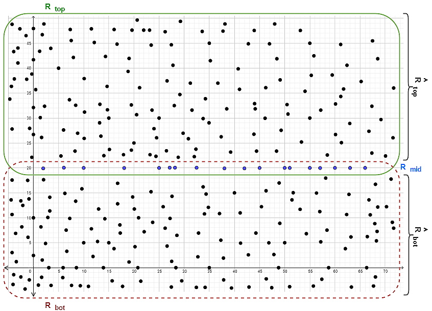
Figure 1: Vehicular network $G^{P}$ range partition around $Y_{mid}=20$

If one of the selected queries does not return a response (i.e. it contains less than $k$ vehicles), we re-select $Y_{mid}$ and repeat the process until all 5 queries are answered (such a value $Y_{mid}$ should exists due to the size of $n$ and the probable distribution of vehicles).

Using the results $S_{top},S_{bot},\hat{S}_{top},\hat{S}_{bot},S_{n}$ we wish to find the average speed of vehicles in section $S_{mid}=F_{avg}(R^{P}_{mid},T)$, and the number of vehicles in each section: $R^{P}_{top},R^{P}_{bot},\hat{R}^{P}_{top},\hat{R}^{P}_{bot},R^{P}_{mid}$. The number of vehicles in each section is a function of the section range and a given timestamp: $C(R,\tau)$. We denote the number of vehicles in each section as follows:

1. $T=C(R^{P}_{top},\tau)$.

2. $B=C(R^{P}_{bot},\tau)$.

3. $M=C(R^{P}_{mid},\tau)$.

4. $\hat{T}=C(\hat{R}^{P}_{top},\tau)=T-M$.

5. $\hat{B}=C(\hat{R}^{P}_{bot},\tau)=B-M$.

To do so, we solve the following equation system:

• $n\cdot S_{n}=B\cdot S_{bot}+T\cdot S_{top}-M\cdot S_{mid}$.

• $B+T-M=n$.

• $T\cdot S_{top}=\hat{T}\cdot\hat{S}_{top}+M\cdot S_{mid}=(T-M)\cdot\hat{S}_{top}+M\cdot S_{mid}$.

• $B\cdot S_{bot}=\hat{B}\cdot\hat{S}_{bot}+M\cdot S_{mid}=(B-M)\cdot B\cdot\hat{S}_{bot}+M\cdot S_{mid}$.

Solving this system gives us the following:

• $B=\frac{n\cdot(S_{n}-\hat{S}_{top})}{S_{bot}-\hat{S}_{top}}$.

• $T=\frac{n\cdot(S_{n}-\hat{S}_{bot})}{S_{top}-\hat{S}_{bot}}$.

• $M=\frac{n\cdot[S_{n}\cdot(\hat{S}_{top}+\hat{S}_{bot}-S_{bot}-S_{top})+S_{bot}\cdot S_{top}-\hat{S}_{bot}\cdot\hat{S}_{top}]}{(\hat{S}_{bot}-S_{top})\cdot S_{bot}+(S_{top}-\hat{S}_{bot})\cdot\hat{S}_{bot}}$.

• $S_{mid}=\frac{(\hat{S}_{bot}\cdot\hat{S}_{top}-S_{bot}\cdot S_{top})\cdot S_{n}}{S_{bot}\cdot S_{top}+(\hat{S}_{top}+\hat{S}_{bot}-S_{top}-S_{bot})\cdot S_{n}-\hat{S}_{bot}\cdot\hat{S}_{top}}+\\ \frac{(S_{top}-\hat{S}_{top})\cdot S_{bot}\cdot\hat{S}_{bot}+(S_{bot}-\hat{S}_{bot})\cdot S_{top}\cdot\hat{S}_{top})}{S_{bot}\cdot S_{top}+(\hat{S}_{top}+\hat{S}_{bot}-S_{top}-S_{bot})\cdot S_{n}-\hat{S}_{bot}\cdot\hat{S}_{top}}$.

Denote this process $ALG_{S_{P}}$. The runtime for this algorithm is the equivalent to running 5 queries on the dataset, with the addition of solving above equation system.

With these values we can now attempt Attack(1) and Attack(2): If $M<k$, we have succeeded in Attack(2). If $M>k$, we can run $ALG_{S_{L}}$ on $R^{P}_{mid}$ which represents the boundaries of a linear graph, we can select on any vehicle with $k$ vehicles on either side of it as the target vehicle $v_{target}$ and perform Attack(1). If $M=k$, we cannot complete either attack, so we select a new value $Y_{mid}$ and run $ALG_{S_{P}}$ again. There exists an edge case of graphs where for all values of $y$ that we can choose as $Y_{mid}$, the number of vehicles $M$ will be equal to $k$, in which case we will be unable to perform any attack. This scenario is, however, unlikely in the case of vehicular networks. In addition, since we have the number of vehicles $T$ and $B$ in $R^{P}_{top}$ and $R^{P}_{bot}$ respectively, if these values are sufficiently large in relation to $n$, we can look at these ranges as sub-graphs of $G_{P}$ and run $ALG_{S_{P}}$ on them with $n_{T}=T$ and $n_{B}=B$.
It is easy to see that we can apply the same method used on the two dimensional graph $G_{P}$ on the three dimensional graph $G_{C}$ with some minor modifications as follows. We again select some value $y$ on the $Y$ axis, denote this value $Y_{mid}$, and split $G_{C}$ into 3 ranges (the section above $Y_{mid}$, the section below $Y_{mid}$, and the section containing only $Y_{mid}$). In this instance, these sections are represented as cubes in the following manner:

• $R^{C}_{top}$: $(-\infty,Y_{mid},-\infty),(\infty,\infty,\infty)$.

• $R^{C}_{bot}$: $(-\infty,Y_{mid},-\infty),(\infty,-\infty,\infty)$.

• $R^{C}_{mid}$: $(-\infty,Y_{mid},-\infty),(\infty,Y_{mid},\infty)$.

Similarly, we define $\hat{R}^{C}_{top}$, $\hat{R}^{C}_{bot}$ to be $R^{C}_{top}\cap R^{C}_{mid}$ and $R^{C}_{bot}\cap R^{C}_{mid}$ respectively. Note that after running our five queries on the five sections, we achieve the same linear equations as in the two dimensional case. Solving these equations now leaves us with the average speed over the plane defined by $R^{C}_{mid}$, and the number of vehicles $M$ in this plane. As in the two dimensional case, if $M<k$ we have succeeded in Attack(2). If $M>k$ we now have a sub-graph of $G^{C}$ which constitutes a two dimensional graph $G_{P}$ on which we may be able to perform $ALG_{S_{P}}$. The minimum size $M$ for this to be possible is $M=2k+1k$.
While our results, given as $ALG_{S_{L}},ALG_{S_{P}}$ and $ALG_{S_{C}}$, refer to the average speeds of vehicles in their respective graph placements, they are not limited to speed values. The same methods can be used for any numeric value that can be averaged over a set of vehicles in this manner, such as number of traffic violations a vehicle has accumulated, number of accidents the vehicle has been involved in, and so on. Any of these, when given as averages over a set of vehicles may appear innocent and maintain high level of privacy for an individual in the system. However, as we have shown, an individual’s data can be inferred with minimal effort by employing our methods. Of course, we are also not limited to vehicular networks. Any data set with the same structure of node placement in a graph will yield the same results.

2.3 Analysis of $F_{min},F_{max}$ and $F_{med}$

In this section we look at possible attacks using the minimum, maximum and median value queries over ranges in the graph as defined previously by $F_{min},F_{max}$ and $F_{med}$ respectively. Similar to the case of $F_{avg}$, we define that the queries will not return a result if the target Range $R$ at time $\tau$ contains less than $k$ individual values. In addition, our analysis of potential attacks rests on the following set of assumptions:

• The data set consists of $n$ unique values.

• The value $k$ is known to the attacker.

• In case a result is returned, the number of actual values in $(R,\tau)$ is not known to the attacker.

• If $(R,\tau)$ contains an even number of values, $F_{med}$ returns the lower of the $2$ median values.

• The attacker is limited only to the $F_{min},F_{max}$ and $F_{med}$ queries, but can perform any number of queries over the data set.

For simplicity, we will treat the data set as in the previous section - a linear graph $G_{L}$ representing a snapshot in time $\tau$ of recorded speeds of vehicles in a specified area. A query of type $q$ ($q$ being $min,max$ or $med$) at time $\tau$ over a range beginning at $x_{i}$ and ending at $x_{j}$ (inclusive) will be denoted $F_{q}([x_{i},x_{j}])$.

We note that there are several special cases in which a trivial attack can be performed. We will address these cases before moving on to the general case.

2.3.1 Case 1: Global Min/Max

Since there exist a unique global minimum and global maximum in the graph, it is easy to see that by querying over the entire graph and iteratively decreasing the range until a new minimum/maximum is found, the vehicle with the minimum and maximum speeds can be discovered.

2.3.2 Case 2: $k-local$ Min/Max

Similar to the case of a global min/max, if a vehicle has the local minimum or maximum value with regards to his $k$ nearest neighbors then their speed can be discovered. This is done using the same method as stated for the global min/max. A range consisting of $k+1$ vehicles, with the outer vehicle having a min (max) speed in that group must be found. Once found, decrease the range until a group of size $k$ remains in its bounds. By our $k-local$ definition, the min (max) value now changes, and the attacker knows that the previous value belongs to the vehicle that has been removed from the range. Note that if a such a $k-local$ min/max vehicle exists in the graph, the attacker can find it given enough queries.

2.3.3 Case 3: $k=3$

In this case, since all values are defined to be unique, querying $F_{min},F_{max},F_{med}$ on a range containing exactly $3$ vehicles return $3$ values, each belonging to a specific vehicle. An attacker can query over a single coordinate at the left-most side of the graph and increase the range until a result is returned. The first time a result is returned, the minimum $k=3$ group size has been reached, and the attacker has the speed of each of the $3$ vehicles. Each speed cannot be attributed to a specific vehicle, but we will denote these $3$ values $s_{1},s_{2},s_{3}$. The attacker now decreases the range’s size from the left until no result is returned, this indicates the range now only contains $2$ vehicles. Increasing the range to the right until a result is returned indicates that a new vehicle has been added to the range. Since all values are unique, one of the values $s_{1},s_{2},s_{3}$ will be missing from the results. This belongs to the left-most vehicle from the previous query results. Continuing this method until the entire graph has been scanned will reveal the speeds of each vehicle in the graph.

2.3.4 The General Case: $k\geq 4$

We show that for the general case, there exists a linear placement of vehicles such that at least $1$ vehicle will have a speed whose value will remain hidden from an attacker. Note that if a combination of $F_{min},F_{max},F_{med}$ queries can be used to attain the same results as the query $F_{avg}$, then a privacy attack can be performed in the manner detailed in Section 2.2.1. Hozo et al. [13] devise a method to estimate the average value and variance of a group using knowledge of only the minimum, maximum and median values. However, for the attack described in $ALG_{S_{L}}$ to succeed, the actual average value is required and not just an estimate. We use an adversarial model and show that for any number $n$ of vehicles and any minimal query size $k$, a vehicle arrangement can be created in which the attacker, using any combination of the above mentioned queries, lacks the ability to discover the speed of at least $1$ vehicle. For any value of $k\geq 4$ and $n\geq k$ we prove this for a specific vehicle $v_{1}$ placed at the leftmost occupied coordinate on the $X$ axis (denoted $x_{1}$). For any value of $k\geq 4$ and $n\geq 2k$ we prove this vehicle may be at any coordinate.

Lemma 2.1.

Let $V$ be a set of $n$ vehicles $v_{1},v_{2},\ldots,v_{n}$ positioned along a linear graph at coordinates $x_{1},x_{2},\ldots,x_{n}$ at time $\tau$. If $k\geq 4$, for any value $n\geq k$ there exists a corresponding assignment of speeds $s1,s2,\ldots,s_{n}$, such that the speed $s_{1}$ of $v_{1}$ cannot be determined by any attacker with access to the $F_{min},F_{max}$ and $F_{med}$ queries over the graph.

Proof.

We prove by induction for $k=4$ and $n\geq k$, then extrapolate for $k\geq 4$ and $n\geq k$.

Show Correctness for $k=4,n=4$

With vehicles $v_{1},v_{2},v_{3},v_{4}$ positioned at $x_{1},x_{2},x_{3},x_{4}$, set the values of $s_{1},s_{2},s_{3},s_{4}$ such that $s_{2}>s_{1}>s_{3}>s_{4}$. Since $k=n=4$ the queries will only return results when the range queried contains the range $[x_{1},x_{n}]$. It is easy to see that:

• $F_{min}([x_{1},x_{n}])=s_{4}$.

• $F_{max}([x_{1},x_{n}])=s_{2}$.

• $F_{med}([x_{1},x_{n}])=s_{3}$.

As such, the value $s_{1}$ of $v_{1}$ is never revealed.

Assume Correctness for $k=4,n=N$

Given a set of vehicles $v_{1},v_{2},v_{3},\ldots,v_{N}$ positioned at coordinates $x_{1},x_{2},x_{3},\ldots,x_{N}$, assume there exists an assignment of corresponding speeds $s_{1},s_{2},s_{3},\ldots,s_{N}$ such that $s_{1}$ cannot be determined by an attacker with access to any number of $F_{min},F_{max},F_{med}$ queries with a $k=4$ limitation.

Prove for $k=4,n=N+1$

We assign $s_{1},s_{2},s_{3},\ldots,s_{N}$ such that for the subgraph $[x_{1},x_{N}]$, for $k=4$, the value of $s_{1}$ is never revealed by any query $F_{min},F_{max},F_{med}$. We note $2$ properties regarding $s_{N+1}$ of the node $v_{N+1}$, placed at $(x_{N+1}\mid x_{N+1}>x_{N})$:

1. There exists only $1$ queryable range, $[x_{1},x_{N+1}]$, for which any query will take both $s_{1}$ and $s_{N+1}$ into consideration.

2. Regardless of the value of $s_{N+1}$, the queries $F_{min}([x_{1},x_{N+1}])$ and $F_{max}([x_{1},x_{N+1}])$ cannot return $s_{1}$ as a result. (Otherwise, $s_{1}$ would have been a result of one of the queries over the subgraph $[x_{1},x_{N}]$)

Due to these properties, we must only ensure that the query
$F_{med}([x_{1},x_{N+1}])$ does not return $s_{1}$ as it’s result. Denote $s_{{med}_{N}}$ to be the result of $F_{med}([x_{1},x_{N}])$. If $s_{{med}_{N}}>s_{1}$ then we set $(s_{N+1}\mid s_{N+1}>s_{{med}_{N}})$ so that $F_{med}([x_{1},x_{N+1}])\geq s_{{med}_{N}}>s_{1}$. Conversely, if $s_{{med}_{N}}<s_{1}$ then we set $(s_{N+1}\mid s_{N+1}<s_{{med}_{N}})$ so that $F_{med}([x_{1},x_{N+1}])\leq s_{{med}_{N}}<s_{1}$. We now have an assignment $s_{1},s_{2},s_{3},\ldots,s_{N},s_{N+1}$ such that the value $s_{1}$ cannot be discovered by an attacker.

Extrapolate for $k\geq 4,n\geq k$

The parameter $k$ is defined as the minimum number of vehicles required to be in a range in order for a result to be returned. For any value of $(n\mid n>k)$ increasing the value of $k$ only reduces the number of available queries that will return a result. Since it holds that there exists an assignment $s_{1},s_{2},s_{3},\ldots,s_{n}$ such that $s_{1}$ cannot be discovered for $k=4$, then setting $k=5$ for the same assignment will not give any new information to the attacker and $s_{1}$ will remain unknown. It can be seen that this is true for any value $k$ such that $n\geq k\geq 4$. ∎ While Lemma 2.1 holds for any value of $k\geq 4$ and $n\geq k$, such an assignment, where a specific node is deterministically undiscoverable, is susceptible to prior knowledge attacks. In addition, in most real world cases, the value of $k$ is chosen to be on a level of magnitude lower than $n$ as to allow for many queries. We show that for these cases, specifically any case where $k\geq 4$ and $n\geq 2k$, the vehicle whose speed is never returned by any query can be chosen as any vehicle by the adversary.

Lemma 2.2.

Let $V$ be a set of $n$ vehicles $v_{1},v_{2},\ldots,v_{n}$ positioned along a linear graph at coordinates $x_{1},x_{2},\ldots,x_{n}$ at time $\tau$. If $k\geq 4$, for any value $n\geq 2k$ there exists a corresponding assignment of speeds $s1,s2,\ldots,s_{n}$, such that there exists a node $v_{j}$ with speed $s_{j}$ which cannot be determined by any attacker with access to the $F_{min},F_{max}$ and $F_{med}$ queries over the graph.

Proof.

We prove by induction for $k=4$ and $n\geq 2k$, then extrapolate for $k\geq 4$ and $n\geq 2k$.

Show Correctness for $k=4,n=8$

With vehicles $v_{1},v_{2},v_{3},\ldots,v_{8}$ positioned at $x_{1},x_{2},x_{3},\ldots,x_{8}$, set the values of $s_{1},s_{2},s_{3},\ldots,s_{8}$ such that $s_{8}>s_{4}>s_{3}>s_{7}>s_{6}>s_{1}>s_{2}>s_{5}$. The value of $s_{3}$ cannot be determined by an attacker even by running all possible query combinations on the graph. The results of all such possible queries can be see in Table 1.

Table 1: All Possible Results of $F_{min},F_{max}$ and $F_{mid}$ with $k=4$ and $n=8$.

	Range Containing $4$ Vehicles
	$[x_{1},x_{4}]$	$[x_{2},x_{5}]$	$[x_{3},x_{6}]$	$[x_{4},x_{7}]$	$[x_{5},x_{8}]$
$F_{min}$	$s_{2}$	$s_{5}$	$s_{5}$	$s_{5}$	$s_{5}$
$F_{max}$	$s_{4}$	$s_{4}$	$s_{4}$	$s_{4}$	$s_{8}$
$F_{med}$	$s_{1}$	$s_{2}$	$s_{6}$	$s_{6}$	$s_{6}$

	Range Containing $5$ Vehicles
	$[x_{1},x_{5}]$	$[x_{2},x_{6}]$	$[x_{3},x_{7}]$	$[x_{4},x_{8}]$
$F_{min}$	$s_{5}$	$s_{5}$	$s_{5}$	$s_{5}$
$F_{max}$	$s_{4}$	$s_{4}$	$s_{4}$	$s_{8}$
$F_{med}$	$s_{1}$	$s_{6}$	$s_{7}$	$s_{7}$

	Range Containing $6$ Vehicles
	$[x_{1},x_{6}]$	$[x_{2},x_{7}]$	$[x_{3},x_{8}]$
$F_{min}$	$s_{5}$	$s_{5}$	$s_{5}$
$F_{max}$	$s_{4}$	$s_{4}$	$s_{8}$
$F_{med}$	$s_{1}$	$s_{6}$	$s_{7}$

	Range Containing $7$ Vehicles
	$[x_{1},x_{7}]$	$[x_{2},x_{8}]$
$F_{min}$	$s_{5}$	$s_{5}$
$F_{max}$	$s_{4}$	$s_{8}$
$F_{med}$	$s_{6}$	$s_{7}$

	Range Containing $8$ Vehicles
	$[x_{1},x_{8}]$
$F_{min}$	$s_{5}$
$F_{max}$	$s_{8}$
$F_{med}$	$s_{6}$

Assume Correctness for $k=4,n=(N\mid N\geq 2k$)

Given a set of vehicles $v_{1},v_{2},v_{3},\ldots,v_{N}$ positioned at coordinates $x_{1},x_{2},x_{3},\ldots,x_{N}$, assume there exists an assignment of corresponding speeds $s_{1},s_{2},s_{3},\ldots,s_{N}$ such that there exists some value $s_{j}$ belonging to some vehicle $v_{j}$ at position $x_{j}$, which cannot be determined by an attacker with access to any number of $F_{min},F_{max},F_{med}$ queries under a $k=4$ limitation.

Prove for $k=4,n=(N+1\mid N\geq 2k)$

We assign $s_{1},s_{2},s_{3},\ldots,s_{N}$ such that for the subgraph $[x_{1},x_{N}]$, for $k=4$, there exists some value of $s_{j}$ which is never revealed by any query $F_{min},F_{max},F_{med}$. Assume $s_{j}\in(s_{1},s_{2},s_{3},\ldots,s_{N-3})$. We note $2$ properties regarding $s_{N+1}$ of the node $v_{N+1}$, placed at $(x_{N+1}\mid x_{N+1}>x_{N})$:

1. Regardless of the value of $s_{N+1}$: $\forall x_{i}\mid x_{i}\in[x_{1},x_{j}]\Rightarrow F_{min}([x_{i},x_{N+1}])<s_{j}$. (i.e. $s_{j}$ cannot be the result of any $F_{min}$ query in the range $[x_{1},x_{N+1}]$)

2. regardless of the value of $s_{N+1}$ : $\forall x_{i}\mid x_{i}\in[x_{1},x_{j}]\Rightarrow F_{max}([x_{i},x_{N+1}])>s_{j}$. (i.e. $s_{j}$ cannot be the result of any $F_{max}$ query in the range $[x_{1},x_{N+1}]$)

Therefore, we must only assign $s_{N+1}$ such that it does not cause $s_{j}$ to be the result of any $F_{med}$ query. Define $s_{{med}_{i}}$ to be the result of $F_{med}([x_{i},x_{N}])$. Due to the properties of $F_{med}$, if $med_{1}>s_{j}$ then $\forall i\mid 1\leq i\leq j\Rightarrow med_{i}>s_{j}$. Conversely, if $med_{1}<s_{j}$ then $\forall i\mid 1\leq i\leq j\Rightarrow med_{i}<s_{j}$. Otherwise at least one of those queries would have returned $s_{j}$ as a result, which contradicts the induction assumption. Define $s_{med}^{\prime}$ to be the closest median value to $s_{j}$ from the previously stated queries.

$$s_{med}^{\prime}=F_{med}([x_{y},x_{N}])\mid\forall i,1\leq i\leq j\Rightarrow|s_{j}-s_{{med}_{i}}|\geq|s_{j}-s_{y}|$$

We set $s_{N+1}$ to be some uniformly distributed random value between $s_{med}^{\prime}$ and $s_{j}$. We now look at $F_{med}([x_{i},x_{N+1}])$ and note that for any value $i\mid 1\leq i\leq j$, the results of $F_{med}([x_{i},x_{N}])$ and $F_{med}([x_{i},x_{N+1}])$ are either the same value or adjacent values, as the speeds in the range differ by exactly $1$ value. Since no value $s_{{med}_{i}}$ is adjacent to $s_{j}$, then $s_{j}$ cannot be the result of any value $F_{med}([x_{i},x_{N+1}],1\leq i\leq j)$. There exist no other queries of the type $f_{med}$ which contain both $x_{j}$ and $x_{N+1}$, therefore we now have an assignment $s_{1},s_{2},s_{3},\ldots,s_{N},s_{N+1}$ such that the value $s_{j}$ cannot be discovered by an attacker.
The above holds for the assumption $s_{j}\in(s_{1},s_{2},s_{3},\ldots,s_{N-3})$. It is easy to see that due to symmetry, the case where $s_{j}\in(s_{4},s_{5},s_{6},\ldots,s_{N})$ allows us to shift all values of $S$ one vehicle to the right, and assign the random value between $s_{med}^{\prime}$ and $s_{j}$ to $s_{1}$. This completes correctness for all positions of $v_{j}$.

Extrapolate for $k\geq 4,n\geq 2k$

Similar to 2.1, increasing $k$ for a given value of $n$ only reduces the amount of information available to the attacker. Therefore, if a value $s_{j}$ exists for an assignment in a graph with $n$ vehicles under the $k=4$ limitation (with $n\geq 2k$), it will exist for any value of $k$ such that $4\leq k\leq\frac{n}{2}$.

∎

3 Collaborative Filtering

Collaborative filtering (CF) is a technique commonly used to build personalized recommendations on the Web. In collaborative filtering, algorithms are used to make automatic predictions about a user’s interests by compiling preferences from several users. In order to provide personalized information to a user, the CF system needs to be provided with sufficient information regarding his or her preferences, behavioral characteristics, as well as demographic information of the individual. The accuracy of the recommendations is dependent largely on how much of this information is known to the CF system. However, this information can prove to be extremely dangerous if it falls in the wrong hands. Several methods aimed at hiding and anonymizing user data have been proposed and studied in an attempt to reduce the privacy issues of collaborative filtering. Among these methods is the data obfuscation technique “Nearest Neighbor Data Substitution” (NeNDS) proposed by Parameswaran and Blough in [2]. Using this approach, items in each column of the database are clustered into groups by closeness of their values, and a substitution algorithm is applied to each group. The algorithm gives each item a new location within the group such that each item now corresponds to a new row in the original database. The relative closeness in values of the substituted items allows for the recommendation system to maintain a good degree of approximation when the CF algorithm is applied to obtain recommendations, while the substitution itself offers a level of privacy by hiding the original values associated with each individual user. In this section, we show the possibility of a privacy attack on the substituted database by an attacker with partial knowledge of the original data.

3.1 The NeNDS Algorithm

The Nearest Neighbor Data Substitution (NeNDS) technique is a lossless data obfuscation technique that preserves the privacy of individual data elements by substituting them with one of their Euclidean space neighbors. NeNDS uses a permutation-based approach in which groups of similar items undergo permutation. The permutation approach hides the original value of a data item by substituting it with another data item that is similar to it but not the same. NeNDs treats each column in the database as a separate dataset. The first step in NeNDS is the creation of similar sets of items called neighborhoods. These items contained in each neighborhood are selected in a manner that maintains Euclidean closeness between neighbors using some distance measuring function suited to the data. Each data set is divided into a pre-specified number of neighborhoods. The items in each neighborhood are then permuted in such a way that each item is displaced from its original position, no two items undergo swapping, and the difference between the values of the original and the obfuscated items is minimal. The number of neighbors in each neighborhood is denoted $NH_{size}$, with $3\leq NH_{size}\leq N$ where $N$ is the number of items in the dataset (this is due to the fact that $NH_{size}=1$ does not allow any permutation and $NH_{size}=2$ is the trivial case of swapping between 2 items and easily reversible).
The substitution process is performed by determining the optimal permutation set subject to the following conditions:

• No two elements in the neighborhood undergo swapping.

• The elements are displaced from their original position.

• Substitution is not performed between duplicate elements.

The permutation mapping is done by creating a tree depicting all possible permutation paths and selecting the path with the minimal maximum distance between any 2 substitutions. For example, we look at the case of the neighborhood $[75,77,82,70]$. The optimal path for substitution would be $70\rightarrow 77\rightarrow 82\rightarrow 75\rightarrow 70$ with the new neighborhood order being $[82,70,77,75]$ and the maximal difference between any 2 substituted items being $(70\rightarrow 77$ and $82\rightarrow 75)$. Once the substitutions in each neighborhood is complete, the column of the original database is replaced with column containing the new item positions. The detailed algorithm can be found in [2]. Note that this algorithm is deterministic for any given value of $NH_{size}$, and will yield the same permutations given any original order of the original dataset.

3.2 Privacy Attack on NeNDS

In this section we will show an attack on a NeNDS permutated database by an attacker with partial knowledge of the original database, specifically the attacker knows the original position of at least $NH_{size}-2$ items in each neighborhood. The attack is performed under the following assumptions:

• The attacker has complete knowledge of the NeNDS algorithm.

• The attacker knows the neighborhood size, $NH_{size}$ used by the algorithm.

• The attacker can measure the Euclidean distance between the items in the database.

• The attacker has access to the output permutated database (i.e. the new positions of all items).

We will show the attack for a single dataset (column), however since the algorithm is performed independently for each dataset, this can be extended to the entire database. For a given dataset of size $n$, we define the following notations:

• Let $X$ be the original dataset $[x_{1},x_{2},\ldots,x_{n}]$.

• Let $Y$ be the NeNDS obfuscated dataset $[y_{1},y_{2},\ldots,y_{n}]$.

• Let $X_{p}$ be the original data items in the $p^{th}$ neighborhood, $[x_{p1},x_{p2},\ldots,x_{pn}]$.

• Let $Y_{p}$ be the obfuscated data items in the $p^{th}$ neighborhood, $[y_{p1},y_{p2},\ldots,y_{pn}]$.

• Let $u_{p1},u_{p2}$ be the 2 items in $X_{p}$ whose original position is unknown to the attacker.

The attack is successful if the attacker can determine the original position in $X$ of $u_{p1}$ and $u_{p2}$ for all values of $p,1\leq p\leq\frac{n}{NH_{size}}$.

3.2.1 The Case of $NH_{size}=3$

We look at the simple case of the minimal neighborhood size, $NH_{size}=3$. In this case, we have for each value of $p$ the neighborhood $[x_{p1},x_{p2},x_{p3}]$. The attacker can only know the location of 1 of these items. Assume, without loss of generality, that the attacker knows the position of $x_{p1}$, and as such the original dataset to be $[x_{p1},u_{p1},u_{p2}]$ where both $u_{p1}$ and $u_{p2}$ could be the original positions of $x_{p2}$ and $x_{p3}$. We now look at the output neighborhood after the NeNDS algorithm. Due to the restrictions of the NeNDS algorithm which require each item to be relocated and do not allow swapping between 2 items, the resulting neighborhood $Y_{p}$ can only be one of the following permutations:

1. $[y_{p1},y_{p2},y_{p3}]=[x_{p2},x_{p3},x_{p1}]$.

2. $[y_{p1},y_{p2},y_{p3}]=[x_{p3},x_{p1},x_{p2}]$.

Any other permutation would entail leaving an item in its original position. Assume permutation (1). The attacker can determine that the value $y_{p1}$ could not have originally been in position $u_{p2}$ since this is the current position of $x_{p1}$ and the algorithm does not allow swapping between 2 items. Therefore, $u_{p2}=x_{p3}$ and $u_{p1}=x_{p2}$. Assume permutation (2). The attacker can determine that the value $y_{p1}$ could not have originally been in position $u_{p1}$ for the same reason, and reaches the same conclusion - the original order for the neighborhood $p$ is $[x_{p1},x_{p2},x_{p3}]$.

3.2.2 The General Case of any $NH_{size}$

In this section we will show that the knowledge of $NH_{size}-2$ original value positions is enough for an attacker to learn the original positions of all $NH_{size}$ values in a neighborhood. We define $L_{o}(x)$ and $L_{n}(x)$ for any value $x\in X$ to be the original and new location (row) of that value respectively. Taking some neighborhood $X_{p}$ in $X$, the attacker knows the position $L_{o}(x_{pi})$ for $NH_{size}-2$ values in $X_{p}$. For 2 values, $u_{p1},u_{p2}$, positions $L_{o}(u_{p1}),L_{o}(u_{p2})$ remain unknown. After obfuscation, all new positions $L_{n}(y_{pi})$ are known to the attacker. With this knowledge, since the values in the neighborhood $X_{p}$ are chosen by their Euclidean closeness, the attacker learns the 2 values $[u_{p1},u_{p2}]$ and their new positions $[L_{n}(u_{p1}),L_{n}(u_{p2})]$. There remain 2 possible original positions $L_{o}(u_{p1}),L_{o}(u_{p2})$ between which the attacker cannot distinguish (i.e. each one of the values could have been at each one of the possible positions originally).
We now examine the new values in $L_{o}(u_{p1}),L_{o}(u_{p2})$. There are 2 cases: either 1 of the values is $u_{p1}$ or $u_{p2}$, or both values are from the other values in $X_{p}$ whose original position is known to the attacker. Note that the case $L_{o}(u_{p1})=L_{n}(u_{p2}),L_{o}(u_{p2})=L_{n}(u_{p1})$ cannot exist since by definition of the algorithm, no 2 items undergo swapping. We now show the attack for both cases, resulting in the discovery of the original positions for $u_{p1},u_{p2}$.

Case 1

Assume, without loss of generality, that $u_{p1}$ resides in a position whose original value is unknown, meaning was either $u_{p1}$ or $u_{p2}$. It is easy to see that $L_{n}(u_{p1})=L_{o}(u_{p2})$ since no item remains in the same position after obfuscation. In addition, the remaining unknown position is $L_{o}(u_{p}1)$. The attacker now knows the original position of both previously unknown values.

Case 2

In this case, both $L_{o}(u_{p1})$ and $L_{o}(u_{p2})$ now contain values whose original position were known to the attacker. We arbitrarily define those positions to be $L_{1}$ and $L_{2}$ and their original values $u_{1}$ and $u_{2}$ respectively. The attacker can know use the following method to backtrack the obfuscation path and find the original positions of $u_{p1}$ and $u_{p2}$. We look at the value currently in $L_{1}$ and denote this value $y_{p1}$. This was the item in the obfuscation path immediately before $u_{1}$. $L_{o}(y_{p1})$ is known to the attacker and contains the value that was in the obfuscation path before $y_{p1}$. Denote this value $y_{p2}$. We now continue this backtracking of the path by examining the value in $L_{o}(y_{p2})$ and so on until we reach on of the values $u_{p1},u_{p2}$. Since the path is created using a tree structure which contains no cycles, the first unknown value we will find must correspond to $u_{2}$ (as $u_{1}$ will be that last item found in our backtracking and complete the path). Assume, without loss of generality, that $u_{2}=u_{p1}$. The attacker now knows that $L_{2}=L_{o}(u_{p1})$ and vice versa.

3.3 NeNDS Shortcomings

In addition to being susceptible to partial knowledge reconstruction, the NeNDS algorithm has an exponential runtime which is not suitable for real world applications. It can be shown the NeNDS algorithm solves the Bottleneck Traveling Salesman problem (BTSP), which is known to be NP-Complete in the general case. For some cases of a defined distance function between values in the database, such as in the case of one dimensional Euclidean distance, there exists a polynomial time solution producing the same results as the NeNDS algorithm (see Figure 2 and Table 2).

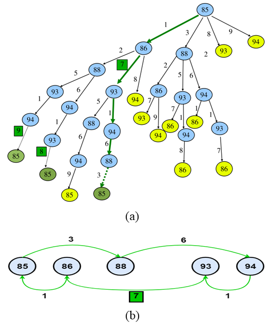
Figure 2: Comparison of NeNDS original algorithm to bottleneck TSP for linear networks. (a) NeNDS tree algorithm - exponential runtime. (b) Bottleneck TSP on linear graph - linear runtime.

Table 2: NeNDS transformation result table - same for both algorithms.

Row	Original Value	Transformed Value
$1$	$86$	$93$
$2$	$88$	$85$
$3$	$93$	$94$
$4$	$85$	$86$
$5$	$94$	$88$

In the general case, there are approximation algorithms for BTSP, such as given by Kao and Sanghi [14] that can be adapted for the case of NeNDS-like perturbation, giving the same level of privacy while achieving an approximate level of accuracy.

4 Conclusions

With more and more user data being stored by companies and organizations, and a growing demand to disseminate and share this data, the risks to security and privacy rise greatly. While some of these issues have been addressed with encryption and authorization protocols, the potential for misuse of access still exists. The need for protecting user privacy while still maintaining utility of databases has given birth to a wide variety of data anonymization techniques. In this research we have analyzed the behavior, vulnerabilities and shortcomings of instances of the data perturbation and the query-set-size control methods. For query-set-size control over a vehicular network (graph based dataset) we have shown the aggregate average query function to be vulnerable to private data leakage. On the other hand, the amalgamation of the minimum, maximum and median query functions allow for user privacy under the examined model. For the case of data perturbation we have presented a partial knowledge attack on the NeNDS algorithm. In addition, we prove the exponential runtime of this algorithm and offer an alternative for the linear coordinate case.
We plan on continued exploration of the privacy attacks described in Section 2. We look to find an upper limit on the number of allowed queries that will reduce the possibility of leaking private information. Other directions in this area include analyzing this query behavior with regards to different data structures, data types and query types. With regards to the attack described in Section 3.2, we intend to look for possibilities of adding randomness to the base permutation of the original data, in order to improve the privacy afforded by NeNDS. This may entail selecting different random values for each $NH_{size}$ and using a non-deterministic, non-optimal permutation algorithm for column transformation, and could come at the cost of a minor loss of data accuracy.

References

- [1] Nabil R. Adam and John C. Worthmann. Security-control methods for statistical databases: A comparative study. ACM Comput. Surv., 21(4):515–556, December 1989.
- [2] Rupa Parameswaran and Douglas M. Blough. Privacy preserving collaborative filtering using data obfuscation. In Proceedings of the 2007 IEEE International Conference on Granular Computing, GRC ’07, pages 380–386, Washington, DC, USA, 2007. IEEE Computer Society.
- [3] Cynthia Dwork, Frank McSherry, Kobbi Nissim, and Adam Smith. Calibrating noise to sensitivity in private data analysis. In Shai Halevi and Tal Rabin, editors, Theory of Cryptography, pages 265–284, Berlin, Heidelberg, 2006. Springer Berlin Heidelberg.
- [4] A. D. Sarwate and K. Chaudhuri. Signal processing and machine learning with differential privacy: Algorithms and challenges for continuous data. IEEE Signal Processing Magazine, 30(5):86–94, Sep. 2013.
- [5] Jaewoo Lee and Chris Clifton. How much is enough? choosing for differential privacy. In Xuejia Lai, Jianying Zhou, and Hui Li, editors, Information Security, pages 325–340, Berlin, Heidelberg, 2011. Springer Berlin Heidelberg.
- [6] Xiaoyuan Su and Taghi M. Khoshgoftaar. A survey of collaborative filtering techniques. Adv. in Artif. Intell., 2009:421425:1–421425:19, January 2009.
- [7] Huseyin Polat and Wenliang Du. Privacy-preserving collaborative filtering using randomized perturbation techniques. In Proceedings of the Third IEEE International Conference on Data Mining, ICDM ’03, pages 625–628, Washington, DC, USA, 2003. IEEE Computer Society.
- [8] Javier Parra-Arnau, David Rebollo-Monedero, and Jordi Forné. A Privacy-Protecting Architecture for Collaborative Filtering via Forgery and Suppression of Ratings, pages 42–57. Springer Berlin Heidelberg, Berlin, Heidelberg, 2012.
- [9] John Canny. Collaborative filtering with privacy via factor analysis. In Proceedings of the 25th Annual International ACM SIGIR Conference on Research and Development in Information Retrieval, SIGIR ’02, pages 238–245, New York, NY, USA, 2002. ACM.
- [10] Zhengli Huang, Wenliang Du, and Biao Chen. Deriving private information from randomized data. In Proceedings of the 2005 ACM SIGMOD International Conference on Management of Data, SIGMOD ’05, pages 37–48, New York, NY, USA, 2005. ACM.
- [11] Hillol Kargupta, Souptik Datta, Qi Wang, and Krishnamoorthy Sivakumar. On the privacy preserving properties of random data perturbation techniques. In Proceedings of the Third IEEE International Conference on Data Mining, ICDM ’03, pages 99–106, Washington, DC, USA, 2003. IEEE Computer Society.
- [12] Giridhair Venkatadri, Athanasios Andreou, Yabing Liu, Alan Mislove, Krishna P. Gummadi, Patrick Loiseau, and Oana Goga. Privacy risks with facebook’s pii-based targeting: Auditing a data brokers advertising interface. In 2018 IEEE Symposium on Security and Privacy (SP), volume 00, pages 89–197, 2018.
- [13] Stela Pudar Hozo, Benjamin Djulbegovic, and Iztok Hozo. Estimating the mean and variance from the median, range, and the size of a sample. BMC Medical Research Methodology, 5(1):13, Apr 2005.
- [14] Ming-Yang Kao and Manan Sanghi. An approximation algorithm for a bottleneck traveling salesman problem. In Tiziana Calamoneri, Irene Finocchi, and Giuseppe F. Italiano, editors, Algorithms and Complexity, pages 223–235, Berlin, Heidelberg, 2006. Springer Berlin Heidelberg.