Article Effect of Inertia on Linear Viscoelasticity
of Harmonic Dumbbell Model

Abstract

The overdamped (inertialess) dumbbell model is widely utilized to study rheological properties of polymers or other soft matters. In most cases, the effect of inertia is merely neglected because the momentum relaxation is much faster than the bond relaxation. We theoretically analyze the effect of inertia on the linear viscoelasticity of the harmonic dumbbell model. We show that the momentum and bond relaxation modes are kinetically coupled and the inertia can affect the bond relaxation if the momentum relaxation is not sufficiently fast. We derive an overdamped Langevin equation for the dumbbell model, which incorporates the weak inertia effect. Our model predicts the bond relaxation dynamics with the weak inertia effect correctly. We discuss how the weak inertia affects the linear viscoelasticity of a simple harmonic dumbbell model and the Rouse model.

1 Introduction

To study molecular-level dynamics of polymers or other soft matters, simple Langevin equation models are useful. From the viewpoint of rheology, the dynamics of molecular-level microscopic degrees of freedom can be related to the macroscopic rheological functions such as the shear relaxation modulus. For example, simple models such as the Rouse model and the reptation model[1] can reproduce experimentally obtained shear relaxation modulus data, and provide the insights on the dynamics of polymers which cannot be directly observed by microscopes.

In many cases, the overdamped Langevin equations without the inertia terms are employed as the dynamic equations for polymers or soft matters. This treatment is reasonable because the dynamical modes related to the inertia (momentum relaxation modes) relax rapidly. If we are interested in relatively long-time scales, we can assume that the inertia effect is not important, and simply take the overdamped (or inertialess) limit. For example, the mean-square displacement (MSD) of a Brownian particle (which obeys the Ornstein-Uhlenbeck process[2]) shows ballistic behavior at the short-time scale. But except the short-time scale region, the MSD can be well approximated by a simple diffusion motion without inertia. However, the effect of the inertia on the dynamics is generally not so simple[3, 4]. The underdamped Langevin equations with the inertia terms are the second order differential equations whereas the overdamped Langevin equations are first order ones. The difference of the differential orders qualitatively affects some properties of the model. Therefore it is important to understand the effect of the inertia on the dynamics.

Here we limit ourselves to one of the simplest model, so-called the dumbbell model[5, 6]. Some researchers have investigated the effects of the inertia on rheological properties of the dumbbell model[7, 8, 9, 10, 11]. Roughly speaking, the overdamped Langevin equations are justified when the inertia effect is very weak. Fortunately, this condition is satisfied for many of polymeric solutions[8, 11], and thus the overdamped Langevin equations can be safely utilized to describe the dynamics. However, this does not mean that the overdamped Langevin equations are always justified. For example, if we model the relaxation process of relatively small objects such as segments, or if we consider the higher order Rouse modes (which essentially behave as statistically independent multiple dumbbell models), the inertia effect may not be simply neglected.

In this work, we investigate the effect of the inertia on the linear viscoelasticity of a simple dumbbell type model. We first derive the approximate Langevin equation for the dumbbell model which is valid for the weak (but non-zero) inertia case. Starting from the underdamped Langevin equation with the inertia term, we show that an overdamped Langevin equation with the lowest order correction by the inertia can be obtained. The dynamics is slightly accelerated by the inertia. Then we apply the obtained approximate dynamic equation to the harmonic dumbbell for which we can obtain analytic solutions. We calculate the shear relaxation modulus and the longest relaxation time, with and without approximations, and discuss how the inertia affects the linear viscoelasticity. We also discuss how the inertia effect accelerates the Rouse model, and a similar acceleration effect by the memory effect in the generalized Langevin equation.

2 Theory

2.1 Model

We start from a dumbbell model[5, 6] with an arbitrary bond potential and the inertial terms. We assume that a dumbbell consists of two beads with the same mass, $M$. We describe the positions and momentum of two beads as $\bm{R}_{1}$ and $\bm{R}_{2}$, and $\bm{P}_{1}$ and $\bm{P}_{2}$, respectively. The Hamiltonian is

$$\mathcal{H}=\frac{1}{2M}(\bm{P}_{1}^{2}+\bm{P}_{2}^{2})+U(\bm{R}_{1}-\bm{R}_{2}),$$ (1)

where $U(\bm{R}_{1}-\bm{R}_{2})$ is the bond potential (which is a harmonic function in the case of the harmonic dumbbell model). If we employ the Langevin thermostat to control the temperature of the system, the dynamic equations for the dumbbell is given as:

$$\frac{d\bm{R}_{i}(t)}{dt} =\frac{1}{M}\bm{P}_{i}(t),$$ (2)

$$\frac{d\bm{P}_{i}(t)}{dt} =-\frac{\partial U(\bm{R}_{1}-\bm{R}_{2}(t))}{\partial\bm{R}_{i}(t)}-\frac{Z}{M}\bm{P}_{i}(t)+\sqrt{2Zk_{B}T}\bm{W}_{i}(t),$$ (3)

for $i=1$ and $2$. Here, $Z$ is the friction coefficient for a bead, $k_{B}$ is the Boltzmann constant, $T$ is the temperature, and $\bm{W}_{i}(t)$ is a Gaussian white noise. The first and second moments of the noise is given as follows:

$$\langle\bm{W}_{i}(t)\rangle=0,\qquad\langle\bm{W}_{i}(t)\bm{W}_{j}(t^{\prime})\rangle=\delta_{ij}\bm{1}\delta(t-t^{\prime}),\qquad$$ (4)

where $\langle\dots\rangle$ represents the statistical average and $\bm{1}$ is the unit tensor.

We may rewrite the dynamic equation by introducing the center of mass $\bar{\bm{R}}\equiv(\bm{R}_{1}+\bm{R}_{2})/2$ and the bond vector $\bm{r}\equiv\bm{R}_{2}-\bm{R}_{1}$. We describe the momenta for the center of mass and the bond vector as $\bar{\bm{P}}\equiv\bm{P}_{1}+\bm{P}_{2}$ and $\bm{p}\equiv(\bm{P}_{2}-\bm{P}_{1})/2$. The Hamiltonian (1) can be rewritten as

$$\mathcal{H}=\frac{1}{2\bar{M}}\bar{\bm{P}}^{2}+\frac{1}{2m}\bm{p}^{2}+U(\bm{r}),$$ (5)

with the total mass $\bar{M}\equiv 2M$ and the reduced mass $m\equiv M/2$. Then we have statistically independent two set of dynamic equations:

$$\frac{d\bar{\bm{R}}(t)}{dt} =\frac{1}{\bar{M}}\bar{\bm{P}}(t),$$ (6)

$$\frac{d\bar{\bm{P}}(t)}{dt} =-\frac{\bar{Z}}{\bar{M}}\bar{\bm{P}}(t)+\sqrt{2\bar{Z}k_{B}T}\bar{\bm{W}}(t),$$ (7)

and

$$\frac{d\bm{r}(t)}{dt} =\frac{1}{m}\bar{\bm{p}}(t),$$ (8)

$$\frac{d\bm{p}(t)}{dt} =-\frac{\partial U(\bm{r}(t))}{\partial\bm{r}(t)}-\frac{\zeta}{m}\bm{p}(t)+\sqrt{2\zeta k_{B}T}\bm{w}(t),$$ (9)

where $\bar{Z}\equiv 2Z$, $\zeta=Z/2$, $\bar{\bm{W}}(t)\equiv(\bm{W}_{1}(t)+\bm{W}_{2}(t))/\sqrt{2}$ and $\bm{w}(t)\equiv(\bm{W}_{2}(t)-\bm{W}_{1}(t))/\sqrt{2}$. Here, it should be noticed that $\bar{\bm{W}}(t)$ and $\bm{w}(t)$ are statistically independent Gaussian white noises, and both of them have the zero mean and unit variance (in the same way as eq (4)).

At the overdamped limit, we set $d\bar{\bm{P}}/dt=0$ and $d\bm{p}/dt$ = 0 in eqs (7) and (9). Then eqs (6)-(9) reduce to the well-known dynamic equations for the fully overdamped dumbbell model:

$$\frac{d\bar{\bm{R}}(t)}{dt} =\sqrt{\frac{2k_{B}T}{\bar{Z}}}\bar{\bm{W}}(t),$$ (10)

$$\frac{d\bm{r}(t)}{dt} =-\frac{1}{\zeta}\frac{\partial U(\bm{r}(t))}{\partial\bm{r}(t)}+\sqrt{\frac{2k_{B}T}{\zeta}}\bm{w}(t).$$ (11)

This approximation is usually justified due to the fact that the characteristic relaxation time of the inertia, $\tau_{m}\equiv m/\zeta=\bar{M}/\bar{Z}$, is much faster than that of the bond (by the competition between the restoring force and the friction force). The momentum relaxation time is common for the center of mass and the bond. Various properties including the linear viscoelasticity of eqs (10) and (11) have been studied, and can be found in literates[5, 6]. The center of mass motion does not contribute to the linear viscoelasticity, and the linear viscoelasticity is fully determined by eq (11). The properties of the overdamped dumbbell model with various bond potential models such as the finitely extensible nonlinear elasticity (FENE) model have been studied extensively[5, 6].

2.2 Approximation for Weak Inertia Case

To investigate the effect of the inertia, we consider an approximate dynamic equation which is valid for small $\tau_{m}=m/\zeta$. We rewrite eqs (8) and (9) as the second order stochastic differential equation for $\bm{r}$:

$$m\frac{d^{2}\bm{r}(t)}{dt^{2}}=-\frac{\partial U(\bm{r}(t))}{\partial\bm{r}(t)}-\zeta\frac{d\bm{r}(t)}{dt}+\sqrt{2\zeta k_{B}T}\bm{w}(t).$$ (12)

We want a first order stochastic differential equation as an approximate form for eq (12). For this purpose, we further rewrite eq (12) as

$$\frac{d\bm{r}(t)}{dt}=\left(1+\tau_{m}\frac{d}{dt}\right)^{-1}\left[-\frac{1}{\zeta}\frac{\partial U(\bm{r}(t))}{\partial\bm{r}(t)}+\sqrt{\frac{2k_{B}T}{\zeta}}\bm{w}(t)\right],$$ (13)

where $(1+\tau_{m}d/dt)^{-1}$ is the inverse operator of $(1+\tau_{m}d/dt)$, and is defined via the following relation for a given function $f(t)$:

$$\left(1+\tau_{m}\frac{d}{dt}\right)^{-1}\left[\left(1+\tau_{m}\frac{d}{dt}\right)f(t)\right]=f(t).$$ (14)

For small $\tau_{m}$, the operator can be expanded into the power series of $\tau_{m}$, and thus we have a simple approximate form, $(1+\tau_{m}d/dt)^{-1}\approx 1-\tau_{m}d/dt$. (We retain only the first order term in $\tau_{m}$.) Then we have the approximate form for the dynamic equation (13) as

$$\begin{split}\frac{d\bm{r}(t)}{dt}&\approx-\frac{1}{\zeta}\frac{\partial U(\bm{r}(t))}{\partial\bm{r}(t)}+\sqrt{\frac{2k_{B}T}{\zeta}}\left(1+\tau_{m}\frac{d}{dt}\right)^{-1}\bm{w}(t)\\ &\qquad+\frac{\tau_{m}}{\zeta}\left[\bm{K}(\bm{r}(t))\cdot\frac{d\bm{r}(t)}{dt}+\frac{k_{B}T}{\zeta}\frac{\partial}{\partial\bm{r}(t)}\cdot\bm{K}(\bm{r}(t))\right],\end{split}$$ (15)

where $\bm{K}(\bm{r})$ is the potential curvature tensor defined as

$$\bm{K}(\bm{r})\equiv\frac{\partial^{2}U(\bm{r})}{\partial\bm{r}\partial\bm{r}},$$ (16)

and we have utilized the Ito formula[12] to calculate $(d/dt)\partial U(\bm{r}(t))/\partial\bm{r}(t)$. In eq (15), we have terms which contain $d\bm{r}(t)/dt$ in both sides. Rearranging these terms and we have

$$\begin{split}\frac{d\bm{r}(t)}{dt}&\approx-\frac{\bm{\Lambda}(\bm{r}(t))}{\zeta}\cdot\frac{\partial U(\bm{r}(t))}{\partial\bm{r}(t)}+\frac{k_{B}T}{\zeta}\frac{\partial}{\partial\bm{r}(t)}\cdot\bm{\Lambda}(\bm{r}(t))\\ &\qquad+\sqrt{\frac{2k_{B}T}{\zeta}}\bm{\Lambda}(\bm{r}(t))\cdot\left(1+\tau_{m}\frac{d}{dt}\right)^{-1}\bm{w}(t),\end{split}$$ (17)

with the effective (dimensionless) mobility tensor defined as

$$\bm{\Lambda}(\bm{r})\equiv\bm{1}+\frac{\tau_{m}}{\zeta}\bm{K}(\bm{r})=\bm{1}+\frac{\tau_{m}}{\zeta}\frac{\partial^{2}U(\bm{r})}{\partial\bm{r}\partial\bm{r}}.$$ (18)

The third term in the right-hand side of eq (17) can be interpreted as the random noise. This noise is not well-defined (due to the fact that time derivative of the noise $\bm{w}(t)$ is not well-defined) and the fluctuation-dissipation relation seems not to be satisfied. It would be natural for us to require the thermodynamic equilibrium state can be correctly realized by the approximate dynamic equation. This requirement can be achieved by modifying the noise term in eq (17) to recover the fluctuation-dissipation relation. (Here, it should be noticed that such an ad-hoc modification cannot be fully justified in general. For the case of the harmonic dumbbell, however, the noise property does not directly affect the linear viscoelasticity. Thus this approximation is not bad for the analyses in what follows.) Finally, we have the following overdamped Langevin equation as an approximate dynamic equation:

$$\frac{d\bm{r}(t)}{dt}=-\frac{\bm{\Lambda}(\bm{r}(t))}{\zeta}\cdot\frac{\partial U(\bm{r}(t))}{\partial\bm{r}(t)}+\frac{k_{B}T}{\zeta}\frac{\partial}{\partial\bm{r}(t)}\cdot\bm{\Lambda}(\bm{r}(t))+\sqrt{\frac{2k_{B}T}{\zeta}}\bm{B}(\bm{r}(t))\cdot\bm{w}(t),$$ (19)

with $\bm{B}(\bm{r})$ being the noise coefficient matrix which satisfies $\bm{B}(\bm{r})\cdot\bm{B}^{\mathrm{T}}(\bm{r})=\bm{\Lambda}(\bm{r})$. Eq (19) is the approximate dynamic equation where the inertia effect is weak, but not absent. Even at the long-time scale, eq (19) does not reduce to eq (11). Only at the fully overdamped case where $\tau_{m}=0$ (or $m=0$), the mobility tensor simply becomes the unit tensor ($\bm{\Lambda}(\bm{r})=\bm{1}$) and eq (19) reduces to eq (11). The fact that the overdamped limit corresponds to the inertialess case ($m=0$) is consistent with the result obtained by Schieber and Öttinger[9].

2.3 Harmonic Dumbbell Model

Here we consider the linear viscoelasticity of the harmonic dumbbell model with the inertia effect and study how the inertia affects the linear viscoelasticity. We set $U(\bm{r})=k\bm{r}^{2}/2$ and assume that the spring constant $k$ satisfies $4km<\zeta^{2}$. (This condition is required to suppress the oscillatory behavior, which is out of the scope of the current work.) At the fully overdamped case where $m=0$, the shear relaxation modulus simply reduces to the single-mode Maxwell model:

$$G(t)=\nu k_{B}Te^{-2t/\tau_{b}},$$ (20)

where $\nu$ is the number density of the dumbbell and $\tau_{b}\equiv\zeta/k$ is the bond relaxation time. In this subsection, we consider how the shear relaxation modulus deviates from eq (20) in the presence of the inertia effect.

We start from the exact solution for the case of the underdamped dumbbell model. The stress of the single harmonic dumbbell can be expressed as the Kramers form:

$$\begin{split}\hat{\bm{\sigma}}(\{\bm{R}_{i}\},\{\bm{P}_{i}\})&\equiv k(\bm{R}_{2}-\bm{R}_{1})(\bm{R}_{2}-\bm{R}_{1})-\frac{1}{M}(\bm{P}_{1}\bm{P}_{1}+\bm{P}_{2}\bm{P}_{2})\\ &=k\bm{r}\bm{r}-\frac{1}{\bar{M}}\bar{\bm{P}}\bar{\bm{P}}-\frac{1}{m}\bm{p}\bm{p}.\end{split}$$ (21)

Then, the shear relaxation modulus is given by the auto-correlation function of the stress tensor, by the Green-Kubo formula[13]:

$$G(t)=\frac{\nu}{k_{B}T}\left\langle\hat{\sigma}_{xy}(t)\hat{\sigma}_{xy}(0)\right\rangle.$$ (22)

Here $\hat{\sigma}_{xy}(t)$ represents the $xy$ component of the stress tensor (21) at time $t$. From eqs (21) and (22), the shear relaxation modulus for the harmonic dumbbell can be expressed in terms of correlation functions. Because $\bar{\bm{P}}$ is statistically independent of $\bm{r}$ and $\bm{p}$, and the system is isotropic, the expression for the relaxation modulus can be simplified as

$$\begin{split}G(t)&=\frac{\nu}{k_{B}T}\bigg{[}\frac{1}{\bar{M}^{2}}\langle\bar{P}_{x}(t)\bar{P}_{x}(0)\rangle^{2}+\frac{1}{m^{2}}\langle p_{x}(t)p_{x}(0)\rangle^{2}+k^{2}\langle r_{x}(t)r_{x}(0)\rangle^{2}\\ &\qquad-\frac{k}{m}\left[\langle r_{x}(t)p_{x}(0)\rangle^{2}+\langle p_{x}(t)r_{x}(0)\rangle^{2}\right]\bigg{]}.\end{split}$$ (23)

Here we have utilized some relations for correlation functions such as $\langle r_{y}(t)r_{y}(0)\rangle=\langle r_{x}(t)r_{x}(0)\rangle$ and $\langle r_{x}(t)r_{y}(0)\rangle=0$.

The correlation function for $\bar{\bm{P}}$ can be easily obtained. From eq (7), we have

$$\langle\bar{\bm{P}}(t)\bar{\bm{P}}(0)\rangle=\bar{M}k_{B}Te^{-t/\tau_{m}}\bm{1},$$ (24)

with $\tau_{m}=\bar{M}/\bar{Z}$ being the momentum relaxation time. Also, the correlation functions for $\bm{r}$ and $\bm{p}$ can be calculated from eqs (8) and (9). For the harmonic potential, the restoring force $-k\bm{r}$ is linear in $\bm{r}$, and we can rewrite eqs (8) and (9) as

$$\frac{d}{dt}\begin{bmatrix}\bm{r}(t)\\ \bm{p}(t)\end{bmatrix}=-\begin{bmatrix}0&-1/m\\ k&\zeta/m\end{bmatrix}\cdot\begin{bmatrix}\bm{r}(t)\\ \bm{p}(t)\end{bmatrix}+\begin{bmatrix}0\\ \sqrt{2\zeta k_{B}T}\bm{w}(t)\end{bmatrix}.$$ (25)

Since eq (25) is linear in $[\bm{r},\bm{p}]^{\mathrm{T}}$, we can solve it by diagonalizing the coefficient matrix. To calculate the linear viscoelasticity, we need the two time correlation functions. The result is:

$$\langle\bm{r}(t)\bm{r}(0)\rangle =\frac{k_{B}T}{k(\lambda_{+}-\lambda_{-})}(\lambda_{+}e^{-\lambda_{-}t}-\lambda_{-}e^{-\lambda_{+}t})\bm{1},$$ (26)

$$\langle\bm{p}(t)\bm{p}(0)\rangle =\frac{mk_{B}T}{\lambda_{+}-\lambda_{-}}(\lambda_{+}e^{-\lambda_{+}t}-\lambda_{-}e^{-\lambda_{-}t})\bm{1},$$ (27)

$$\langle\bm{r}(t)\bm{p}(0)\rangle =-\langle\bm{p}(t)\bm{r}(0)\rangle=\frac{k_{B}T}{\lambda_{+}-\lambda_{-}}(e^{-\lambda_{-}t}-e^{-\lambda_{+}t})\bm{1},$$ (28)

with the eigenvalues of the coefficient matrix defined as

$$\lambda_{\pm}\equiv\frac{\zeta\pm\sqrt{\zeta^{2}-4km}}{2m}.$$ (29)

See Appendix A for the detailed calculations. Eq (29) can be rewritten in terms of the momentum relaxation time $\tau_{m}=m/\zeta$ and the bond relaxation time $\tau_{b}=\zeta/k$:

$$\lambda_{\pm}=\frac{1\pm\sqrt{1-4\tau_{m}/\tau_{b}}}{2\tau_{m}},$$ (30)

and if two relaxation times are well separated, $\tau_{b}\gg\tau_{m}$, we can approximate eigenvalues as $\lambda_{+}\approx 1/\tau_{m}$ and $\lambda_{-}\approx(1+\tau_{m}/\tau_{b})/\tau_{b}$.

By substituting eqs (24) and (26)-(28) into eq (23), we finally have the explicit expression for the relaxation modulus:

$$G(t)=\nu k_{B}T\left[e^{-2t/\tau_{m}}+e^{-(1+\sqrt{1-4\tau_{m}/\tau_{b}})\,t/\tau_{m}}+e^{-(1-\sqrt{1-4\tau_{m}/\tau_{b}})\,t/\tau_{m}}\right].$$ (31)

The detailed calculations are shown in Appendix A. From eq (31), the relaxation modulus consists of three Maxwell models. At the long-time region, only the longest relaxation mode in eq (31) survives. In addition, if the momentum relaxation is sufficiently fast, $\tau_{b}\gg\tau_{m}$, the relaxation time can be approximated as a simple form. Thus we have the following approximate form:

$$G(t)\approx\nu k_{B}Te^{-2(1+\tau_{m}/\tau_{b})\,t/\tau_{b}}.$$ (32)

Eq (32) is similar to eq (20) but the relaxation time is slightly different. The relaxation time of eq (32) is $\bar{\tau}\equiv\tau_{b}/2(1+\tau_{m}/\tau_{b})$. This relaxation time $\bar{\tau}$ coincides to $\tau_{b}/2$ if $\tau_{m}/\tau_{b}=0$, but it is generally different from $\tau_{b}/2$. Therefore, we conclude that the overdamped limit cannot be justified unless $\tau_{m}/\tau_{b}$ is sufficiently small.

Now we apply the approximate dynamic equation (19) to the harmonic dumbbell case. By substituting $U(\bm{r})=k\bm{r}^{2}/2$ to eqs (16) and (18), we have

$$\bm{K}(\bm{r})=k\bm{1},\qquad\bm{\Lambda}(\bm{r})=\left(1+\frac{\tau_{m}}{\tau_{b}}\right)\bm{1}.$$ (33)

From eq (33), we find that for the harmonic dumbbell model, the mobility tensor is independent of the bond vector $\bm{r}$. Therefore, eq (19) becomes the following overdamped Langevin equation with the additive noise:

$$\frac{d\bm{r}(t)}{dt}=-\frac{1}{\tau_{b}}\left(1+\frac{\tau_{m}}{\tau_{b}}\right)\bm{r}(t)+\sqrt{\frac{2k_{B}T}{\zeta}\left(1+\frac{\tau_{m}}{\tau_{b}}\right)}\bm{w}(t).$$ (34)

Eq (34) is a simple linear Langevin equation (or the Ornstein-Uhlenbeck process[2]), and can be solved easily. From eq (34), we have the correlation function as

$$\langle\bm{r}(t)\bm{r}(0)\rangle=\frac{k_{B}T}{k}e^{-(1+\tau_{m}/\tau_{b})\,t/\tau_{b}}\bm{1}.$$ (35)

The single dumbbell stress tensor is given as the partial average over the momenta for eq (21):

$$\hat{\bm{\sigma}}(\bm{r})=k\bm{r}\bm{r}-2k_{B}T\bm{1},$$ (36)

and the Green-Kubo formula (22) gives the following expression for the relaxation modulus:

$$G(t)=\frac{\nu k^{2}}{k_{B}T}\langle r_{x}(t)r_{x}(0)\rangle^{2}.$$ (37)

Finally, from eqs (35) and (37), we have the following explicit expression for the relaxation modulus:

$$G(t)=\nu k_{B}Te^{-2(1+\tau_{m}/\tau_{b})\,t/\tau_{b}}.$$ (38)

Eq (38) has the same form as eq (32). Therefore, from the approximate dynamic equation (19), we can successfully reproduce the relaxation time $\bar{\tau}=\tau_{b}/2(1+\tau_{m}/\tau_{b})$.

3 Discussions

3.1 Relaxation of Harmonic Dumbbell Model

The long-time dynamics of a Brownian particle with inertia can be well approximated by that without inertia. The diffusion coefficients calculated from the mean square displacement the long-time region, with and without inertia, are exactly the same. Thus for a diffusion process, we can reasonably approximate the underdamped Langevin equation by the overdamped one at the long-time region where $t\gtrsim\tau_{m}$. In contrast, the long-time dynamics of a dumbbell model with inertia does not reduce to that without inertia. The exact expression for the relaxation modulus with inertia (eq (31)) has three relaxation modes: The center of mass momentum relaxation model, the bond momentum relaxation mode, and the bond relaxation mode. The degrees of freedom of the center of mass ($\bar{\bm{R}}$ and $\bar{\bm{P}}$) give only a single mode, which is essentially the same as the relaxation mode of a single Brownian particle. On the other hand, the degrees of freedom of the bond ($\bm{r}$ and $\bm{p}$) have two relaxation modes, unlike the case of the center of mass. The relaxation times of these two modes depend both on the momentum relaxation time $\tau_{m}$ and the bond relaxation $\tau_{b}$. We may interpret that these two modes are kinetically coupled. Thus even at the long-time region, the relaxation time $\bar{\tau}$ depends on both $\tau_{b}$ and $\tau_{m}$.

We show the relaxation modulus of the harmonic dumbbell with the inertia effect ($\tau_{m}/\tau_{b}=0.1$) in Figure 1. At the short-time scale ($t\lesssim\tau_{m}$), we observe the momentum relaxation modes. The modulus at the overdamped limit (eq (20)) deviates from the exact one (eq (31)) even at the long-time region ($t\gtrsim\tau_{b}$). (The deviation seems not large at the logarithmic scale for $\tau_{m}/\tau_{b}=0.1$.) In contrast to the overdamped limit, the approximate form for weak inertia (eq (38)) agrees reasonably with the exact one. Thus we find that the approximate dynamic equation (19) derived in this work is a reasonable approximation where the inertia effect is small but not fully negligible.

To study the effect of the inertia, we consider how the zero shear viscosity $\eta_{0}$ and the longest relaxation time $\tau_{d}$ depend on the ratio $\tau_{m}/\tau_{b}$. From eq (31), the longest relaxation time is $\tau_{d}=\tau_{m}/(1-\sqrt{1-4\tau_{m}/\tau_{b}})$ (for $\tau_{m}/\tau_{b}<1/4$). The zero shear viscosity at the overdamped limit is simply given as $\nu k_{B}T\tau_{b}/2$. On the other hand, from eq (31), the zero shear viscosity with the inertia effet becomes

$$\frac{\eta_{0}}{\nu k_{B}T\tau_{b}/2}=\frac{2\tau_{m}}{\tau_{b}}\left[\frac{1}{2}+\frac{1}{1+\sqrt{1-4\tau_{m}/\tau_{b}}}+\frac{1}{1-\sqrt{1-4\tau_{m}/\tau_{b}}}\right].$$ (39)

Figure 2 shows the $\tau_{m}/\tau_{b}$ dependence of the zero shear viscosity $\eta_{0}$ and the longset relaxation time $\tau_{d}$. (For convenience, $\eta_{0}$ and $\tau_{d}$ are normalized by their overdamped limits.) As $\tau_{m}/\tau_{b}$ increases, the zero shear viscosity increases wheareas the longest relaxation time decreases. The increase of the viscosity is due to two relatively fast relaxation modes (the momentum relxation modes) which disappear at the overdamped limit.

We can understand the effect of the inertia term on the dynamics via the Langevin equation (19). In eq (19), inertia term modulates the the mobility tensor from $\bm{1}$ to $\bm{\Lambda}(\bm{r})$. Intuitively, this can be interpreted as the acceleration effect. The acceleration depends on the curvature tensor $\bm{K}(\bm{r})$ which generally depends on the bond vector $\bm{r}$. In the case of the harmonic potential, the curvature is isotropic and given as a positive constant $k$, and therefore all the dynamics is simply accelerated by the factor $(1+\tau_{m}/\tau_{b})$. This acceleration factor is consistent with the fact that the ratio of the relaxation time $\bar{\tau}$ to one at the overdamped limit $\tau_{b}/2$ is $\bar{\tau}/(\tau_{b}/2)=(1+\tau_{m}/\tau_{b})^{-1}$. If the potential is not harmonic, the acceleration depends on the bond vector. In such a case, the relaxation will be much more complex compared with the harmonic dumbbell model. However, any bond potential potentials will exhibit the acceleration effect on the bond dynamics, on average. Thus we expect that the acceleration of the viscoelastic relaxation time will be common and independent of the details of the bond potential.

3.2 Rouse Model with Inertia Effect

The acceleration effect by the inertia term will be non-negligible if we study relatively small scale relaxation modes. A simple yet nontrivial example is the Rouse model[1]. Usually, the Rouse model is defined as the the overdamped Langevin equation with the free energy for an ideal chain which consists of $N$ beads. For simplicity, we assume that $N$ is sufficiently large. We employ the underdamped Langevin equation instead of the overdamped one:

$$m\frac{d^{2}\bm{R}_{k}(t)}{dt^{2}}=-\frac{\partial\mathcal{F}(\{\bm{R}_{k}(t)\})}{\partial\bm{R}_{k}(t)}-\zeta\frac{d\bm{R}_{k}(t)}{dt}+\sqrt{2\zeta k_{B}T}\bm{w}_{k}(t),$$ (40)

where $\bm{R}_{k}$ represents the position of the $k$-th bead ($k=1,2,\dots,N$), $m$ is the mass of a bead, $\zeta$ is the friction coefficient for a bead, $\mathcal{F}(\{\bm{R}_{k}\})$ is the free energy for an ideal chain, and $\bm{w}_{k}(t)$ is the Gaussian white noise. The free energy is given as

$$\mathcal{F}(\{\bm{R}_{k}\})=\frac{3k_{B}T}{2b^{2}}\sum_{k=1}^{N-1}(\bm{R}_{k+1}-\bm{R}_{k})^{2},$$ (41)

with $b$ being the segment size, and the noise satisfies the following relations:

$$\langle\bm{w}_{k}(t)\rangle=0,\qquad\langle\bm{w}_{k}(t)\bm{w}_{l}(t^{\prime})\rangle=\delta_{kl}\bm{1}\delta(t-t^{\prime}).$$ (42)

By using the Rouse mode defined as $\bm{X}_{p}\equiv\sqrt{2/N}\sum_{k}\cos(p\pi k/N)\bm{R}_{k}$ ($p=1,2,3,\dots$), we can rewrite the dynamic equation (40) as

$$m\frac{d^{2}\bm{X}_{p}(t)}{dt^{2}}=-\frac{\zeta p^{2}}{\tau_{R}}\bm{X}_{p}(t)-\zeta\frac{d\bm{X}_{p}(t)}{dt}+\sqrt{2\zeta k_{B}T}\bm{W}_{p}(t),$$ (43)

where $\tau_{R}\equiv N^{2}b^{2}\zeta/3\pi^{2}k_{B}T$ is the Rouse time and $p=1,2,3,\dots$ is the mode index (we ignore the zeroth mode $p=0$, because it does not contribute to the stress for the weak inertia case). $\bm{W}_{p}(t)$ is the Gaussian white noise which satisfies

$$\langle\bm{W}_{p}(t)\rangle=0,\qquad\langle\bm{W}_{p}(t)\bm{W}_{q}(t^{\prime})\rangle=\delta_{pq}\bm{1}\delta(t-t^{\prime}).$$ (44)

We apply eq (19) to the Rouse model, eq (43). Then, the approximate dynamic equation becomes

$$\frac{d\bm{X}_{p}(t)}{dt}=-\frac{p^{2}}{\tau_{R}}\left(1+\frac{\tau_{m}p^{2}}{\tau_{R}}\right)\bm{X}_{p}(t)+\sqrt{\frac{2k_{B}T}{\zeta}\left(1+\frac{\tau_{m}p^{2}}{\tau_{R}}\right)}\bm{W}_{p}(t),$$ (45)

where $\tau_{m}=m/\zeta$ is the momentum relaxation time. Eq (45) is valid only when the inertia effect is weak. Roughly, this condition is estimated as $p\lesssim p^{*}$, where $p^{*}$ is given as $p^{*}=\sqrt{\tau_{R}/\tau_{m}}=Nb\zeta/(\pi\sqrt{3mk_{B}T})$.

The discussions above implies that we should introduce the cutoff for the index $p$ unless the inertia effect is not fully negligible. In molecular dynamics simulations such as the Kremer-Grest model[14], we usually employ the unit where the mass, energy, and the bead size becomes unity. Other quantities such as the friction coefficient $\zeta$ and the temperature $k_{B}T$ are typically of the order of unity. Then the maximum index $p^{*}$ can be estimated as $p^{*}\approx N/(\pi\sqrt{3})\approx 0.18N$. Thus, we find that only less than $20\%$ of the Rouse modes work as naively expected. (Higher order modes will largely deviate from the prediction of the simple Rouse model.)

Even if the cutoff effect is minor and thus not important, the acceleration by the inertia effect depends on the index $p$. The shear relaxation modulus can deviate from the simple Rouse type behavior. From eq (45), the relaxation modulus becomes

$$G(t)=\nu k_{B}T\sum_{p=1}^{\infty}\exp\left[-\frac{2p^{2}}{\tau_{R}}\left(1+\frac{\tau_{m}p^{2}}{\tau_{R}}\right)t\right],$$ (46)

where $\nu$ is the chain density. Therefore, the longest relaxation time is given as $\bar{\tau}=\tau_{R}/2(1+\tau_{m}/\tau_{R})$. As the case of the harmonic dumbbell, the relaxation is accelerated by the factor of $1+\tau_{m}/\tau_{R}$. For the intermediate time region where $\tau_{m}\lesssim t\lesssim\tau_{R}$, we may replace the discrete sum over $p$ by a continuum integral (as the usual approximation for the Rouse model[1]), we have

$$\begin{split}G(t)&\approx\nu k_{B}T\int_{0}^{\infty}dp\,\exp\left[-\frac{2p^{2}}{\tau_{R}}\left(1+\frac{\tau_{m}p^{2}}{\tau_{R}}\right)t\right]\\ &=\frac{\nu k_{B}T}{4}\sqrt{\frac{\tau_{R}}{\tau_{m}}}e^{t/4\tau_{m}}K_{1/4}\left(\frac{t}{4\tau_{m}}\right)\end{split}$$ (47)

where $K_{1/4}(x)$ is the modified Bessel function of the second kind with the order $1/4$[15]. (The summation over $p$ for $p\geq 1$ in eq (46) is replaced by the integral for $p\geq 0$, not for $p\geq 1$, in eq (47). The integral over the range $0\leq p\leq 1$ is much smaller than that over the range $p\geq 1$, and thus we simply neglected it.) We can analytically calculate the complex modulus of the model based on eq (46) or eq (47). The complex moduli given by eqs (46) and (47) show reasonable agreement, and thus we find that eq (47) works as a good approximation. The detailed calculations are shown in Appendix B. At relatively long-time scale ($\tau_{m}\ll t\lesssim\tau_{R}$), the asymptotic expansion[15] can be utilized and eq (47) can be simplified as

$$G(t)\approx\nu k_{B}T\sqrt{\frac{\pi\tau_{R}}{2t}}\left(1-\frac{3\tau_{m}}{8t}\right).$$ (48)

The first term in the parenthesis in the right-hand side of eq (48) corresponds to the usual (inertialess) Rouse type terms[1], and the second term can be interpreted as the correction. Eqs (47) and (48) imply that the shear relaxation modulus could slightly deviate from the well-known Rouse type behavior $G(t)\propto t^{-1/2}$, if the inertia effect is not sufficiently weak. We show the relaxation modulus by eq (47) (with $\tau_{m}/\tau_{R}=0.01$) together with the usual expression at the fully overdamped limit in Figure 3. For comparison, we show the relaxation modulus data directly calculated with the discrete sum expression, eq (46), with $\tau_{m}/\tau_{R}=0.01$ and $0$. With this parameter setting, the longest relaxation time $\bar{\tau}$ is almost the same as that at the overdamped limit $\tau_{R}/2$ ($\bar{\tau}/(\tau_{R}/2)\approx 0.99$ for $\tau_{m}/\tau_{R}=0.01$). The relaxation modulus by eq (47) looks almost the same as that at the overdamped limit at the relatively long-time region in Figure 3. However, we observe a clear deviation between eq (47) and the overdamped limit at the relatively short-time region. We observe a similar discrepancy for moduli calculated with the discrete sum expression. As the case of the dumbbell model, the inertia effect accelerates the relaxation.

Apparently, these results seem not to be consistent with the fact that the experimental and simulation data of shear relaxation modulus for unentangled polymer melts can be fitted well to the Rouse model[16, 17]. However, we should recall that the polymer chains in melts are strongly interacting with each other by the short-range repulsive interaction between segments, even if they are not entangled. From this point of view, it is not plausible for unentangled polymer melts to obey the simple Rouse model. Also, a recent study on the Langevin equation with a fluctuating diffusivity suggested that the Rouse type relaxation can emerge if the diffusivity (or the friction coefficient) is heterogeneous and fluctuates in time[18]. Therefore, even if the shear relaxation modulus exhibits the Rouse type behavior, we cannot conclude that the molecular level dynamics fully obeys the simple Rouse model. Careful and detailed analyses would be required to further investigate the molecular level dynamics of polymers.

3.3 Memory Effect

To model complex relaxation behavior, the generalized Langevin equation[3, 19, 20] is widely employed. In the generalized Langevin equation, the memory effect is expressed by using a memory kernel. Formally, the generalized Langevin equation is obtained by eliminating the microscopic fast degrees of freedom, and the projection operator formalism[19] gives the expression of the memory kernel. Although, in principle, the memory kernel for a specific system can be determined by the dynamics of the fast degrees of freedom in the system, we cannot calculate its explicit form in most of practical cases. Thus rather phenomoenolgical and simple memory functions such as a single exponential form are employed in some cases. In addition, if the relaxation time of fast degrees of freedom, $\tau_{f}$, is much faster than the characteristic time scale of the slow degrees of freedom, the memory effect may be neglected. (This relaxation time $\tau_{f}$ can be interpreted as the memory relaxation time.) Then the usual Langevin equation can be used as an approximate dynamic equation (the Markovian approximation).

In some aspects, the Markovian approximation explained above is similar to the overdamped limit for the Langevin equation with the inertia effect. Thus it would be informative to discuss how the memory kernel affects the relaxation time of the dumbbell model. Actually, the Langevin equation (12) can be rewritten as the generalized Langevin equation, and thus we can interpret our approximation method as an approximation for the generalized Langevin equation. We introduce the Green function $\Gamma(t)$ for the operator $(1+\tau_{m}d/dt)$:

$$\left(1+\tau_{m}\frac{d}{dt}\right)\Gamma(t)=\delta(t).$$ (49)

It is straightforward to see the following function $\Gamma(t)$ satisfies eq (49) and thus is the Green function:

$$\Gamma(t)=\frac{1}{\tau_{m}}e^{-t/\tau_{m}}\Theta(t),$$ (50)

where $\Theta(t)$ is the Heaviside step function. The application of the operator $(1+\tau_{m}d/dt)^{-1}$ to a given function $f(t)$ can be interpreted as the convolution of $\Gamma(t)$ and $f(t)$:

$$\left(1+\tau_{m}\frac{d}{dt}\right)^{-1}f(t)=\int_{-\infty}^{t}dt^{\prime}\,\Gamma(t-t^{\prime})f(t^{\prime}).$$ (51)

Then eq (12) (or eq (13)) can be exactly rewritten as

$$\frac{d\bm{r}(t)}{dt}=-\frac{1}{\zeta}\int_{-\infty}^{t}dt^{\prime}\,\Gamma(t-t^{\prime})\frac{\partial U(\bm{r}(t^{\prime}))}{\partial\bm{r}(t^{\prime})}+\sqrt{\frac{k_{B}T}{\zeta}}\bm{\xi}(t),$$ (52)

where $\bm{\xi}(t)$ is a Gaussian colored noise which is defined as

$$\bm{\xi}(t)\equiv\sqrt{2}\int_{-\infty}^{t}dt^{\prime}\,\Gamma(t-t^{\prime})\bm{w}(t^{\prime}).$$ (53)

Clearly, the first moment of $\bm{\xi}(t)$ is zero, $\langle\bm{\xi}(t)\rangle=0$. The second moment reduces to a simple form:

$$\begin{split}\langle\bm{\xi}(t)\bm{\xi}(t^{\prime})\rangle&=2\int_{-\infty}^{t}ds\int_{-\infty}^{t^{\prime}}ds^{\prime}\,\Gamma(t-s)\Gamma(t^{\prime}-s^{\prime})\bm{1}\delta(s-s^{\prime})\\ &=\frac{1}{\tau_{m}}\bm{1}e^{-|t-t^{\prime}|/\tau_{m}}=\bm{1}\Gamma(|t|).\end{split}$$ (54)

Eq (54) is nothing but the fluctuation-dissipation relation, and thus we can interpret eq (52) as the generalized Langevin equation with the memory kernel $\Gamma(t)$ given by eq (50).

As we discussed, the inertia effect accelerates the relaxation. This acceleration effect is also caused in the case of the generalized Langevin equation. Therefore, in general, the memory effect may not be fully neglected even if we consider relatively long-time scale dynamics. To reproduce the correct relaxation behavior, we should employ the effective mobility tensor. We expect that the analyses for the weak inertia cases can be used to analyze the dumbbell model with a weak memory effect, by replacing the momentum relaxation time $\tau_{m}$ by the memory relaxation time $\tau_{f}$.

4 Conclusions

In this work, we studied the effect of the inertia on the dynamics of the dumbbell model. We derived the approximate dynamic equation to describe the dynamics for the weak inertia case. The inertia effects modulate the mobility tensor, and thus the dynamics is slightly accelerated. As a result, the dynamical properties such as the shear relaxation modulus deviates from those at the overdamped limit.

As an example, we analyzed the harmonic dumbbell model which can be solved analytically. We calculated the exact expression for the shear relaxation modulus and showed that there are three relaxation modes. One mode is the momentum relaxation of the center of mass, and the other two modes are the momentum relaxation of the bond and the bond relaxation. The relaxation times of two modes for the bond depend both on the momentum relaxation time $\tau_{m}$ and the bond relaxation time $\tau_{b}$. The longest relaxation time is approximated as $\bar{\tau}\approx\tau_{b}/2(1+\tau_{m}/\tau_{b})$, which is different from that at the overdamped limit, $\tau_{b}/2$. On the other hand, the approximate dynamic equation (19) gives the correct long relaxation time. Although the inertia effect may not be important in many practical cases, it can be non-negligible for some limited cases. We consider that the analyses based on the approximate dynamic equation and the detailed and careful analyses of the experimental data will be required when the inertia effect becomes non-negligible.

Appendix

Appendix A Detailed Calculations for Harmonic Dumbbell Model

In this appendix, we show detailed calculations for the harmonic dumbbell model with inertia effect, without approximations. The dynamic equation is given as eq (25) in the main text. We describe the coefficient matrix as

$$\bm{C}\equiv\begin{bmatrix}0&-1/m\\ k&\zeta/m\end{bmatrix}.$$ (55)

$\bm{C}$ has the eigenvalues $\lambda_{\pm}$ in eq (29) and the corresponding eigenvectors are

$$\bm{\psi}_{\pm}\equiv\begin{bmatrix}1\\ -m\lambda_{\pm}\end{bmatrix}.$$ (56)

Then we can diagonalize eq (25) with the transformation matrix $\bm{V}\equiv[\bm{\psi}_{+}\,\bm{\psi}_{-}]$ and its inverse $\bm{V}^{-1}$. Multiplying $\bm{V}^{-1}$ from the left side to eq (25) gives

$$\frac{d}{dt}\bm{V}^{-1}\cdot\begin{bmatrix}\bm{r}(t)\\ \bm{p}(t)\end{bmatrix}=-\begin{bmatrix}\lambda_{+}&0\\ 0&\lambda_{-}\end{bmatrix}\cdot\bm{V}^{-1}\cdot\begin{bmatrix}\bm{r}(t)\\ \bm{p}(t)\end{bmatrix}+\bm{V}^{-1}\cdot\begin{bmatrix}0\\ \sqrt{2\zeta k_{B}T}\bm{w}(t)\end{bmatrix}.$$ (57)

After integrating eq (57) from $0$ to $t$, we multiply $\bm{V}$ to both sides and have

$$\begin{split}\begin{bmatrix}\bm{r}(t)\\ \bm{p}(t)\end{bmatrix}&=\bm{V}\cdot\begin{bmatrix}e^{-\lambda_{+}t}&0\\ 0&e^{-\lambda_{-}t}\end{bmatrix}\cdot\bm{V}^{-1}\cdot\begin{bmatrix}\bm{r}(0)\\ \bm{p}(0)\end{bmatrix}\\ &\qquad+\int_{0}^{t}dt^{\prime}\,\bm{V}\cdot\begin{bmatrix}e^{-\lambda_{+}(t-t^{\prime})}&0\\ 0&e^{-\lambda_{-}(t-t^{\prime})}\end{bmatrix}\cdot\bm{V}^{-1}\cdot\begin{bmatrix}0\\ \sqrt{2\zeta k_{B}T}\bm{w}(t^{\prime})\end{bmatrix}.\end{split}$$ (58)

Now, $\bm{r}(0)$ and $\bm{p}(0)$ are statistically independent of the noise $\bm{w}(t)$ for $t>0$. In addition, in equilibrium, $\bm{r}(0)$ and $\bm{p}(0)$ obey the Boltzmann distribution with the Hamiltonian (5). Thus the averages over $\bm{r}(0),\bm{p}(0)$, and $\bm{w}(t)$ can be took separately. The two time correlation functions for $\bm{r}$ and $\bm{p}$ can be obtained as

$$\begin{split}\left\langle\begin{bmatrix}\bm{r}(t)\bm{r}(0)&\bm{r}(t)\bm{p}(0)\\ \bm{p}(t)\bm{r}(0)&\bm{p}(t)\bm{p}(0)\end{bmatrix}\right\rangle&=\bm{V}\cdot\begin{bmatrix}e^{-\lambda_{+}t}&0\\ 0&e^{-\lambda_{-}t}\end{bmatrix}\cdot\bm{V}^{-1}\cdot\begin{bmatrix}(k_{B}T/k)\bm{1}&0\\ 0&mk_{B}T\bm{1}\end{bmatrix}\\ &=\frac{k_{B}T}{\lambda_{+}-\lambda_{-}}\begin{bmatrix}(\lambda_{+}e^{-\lambda_{-}t}-\lambda_{-}e^{-\lambda_{+}t})/k&e^{-\lambda_{-}t}-e^{-\lambda_{+}t}\\ e^{-\lambda_{+}t}-e^{-\lambda_{-}t}&m(\lambda_{+}e^{-\lambda_{+}t}-\lambda_{-}e^{-\lambda_{-}t})\end{bmatrix}\bm{1},\end{split}$$ (59)

where we have utilized the relation for the eigenvalues, $\lambda_{+}\lambda_{-}=k/m$. Eq (59) gives eqs (26)-(28) in the main text.

The relaxation modulus $G(t)$ can be calculated by eqs (23), (24) and (26)-(28):

$$\begin{split}G(t)&=\nu k_{B}T\bigg{[}e^{-2t/\tau_{m}}+\left(\frac{\lambda_{+}e^{-\lambda_{+}t}-\lambda_{-}e^{-\lambda_{-}t}}{\lambda_{+}-\lambda_{-}}\right)^{2}+\left(\frac{\lambda_{+}e^{-\lambda_{-}t}-\lambda_{-}e^{-\lambda_{+}t}}{\lambda_{+}-\lambda_{-}}\right)^{2}\\ &\qquad-\frac{2}{\tau_{b}\tau_{m}}\left(\frac{e^{-\lambda_{-}t}-e^{-\lambda_{+}t}}{\lambda_{+}-\lambda_{-}}\right)^{2}\bigg{]},\end{split}$$ (60)

where we have utilized the relation $k/m=(k/\zeta)(\zeta/m)=1/\tau_{b}\tau_{m}$. Some factors in eq (60) can be simplified as follows:

$$\frac{1}{(\lambda_{+}-\lambda_{-})^{2}}=\frac{m^{2}}{\zeta^{2}-4km}=\frac{\tau_{m}^{2}}{1-4\tau_{m}/\tau_{b}},$$ (61)

$$\begin{split}&(\lambda_{+}e^{-\lambda_{+}t}-\lambda_{-}e^{-t\lambda_{-}})^{2}+(\lambda_{+}e^{-\lambda_{-}t}-\lambda_{-}e^{-t\lambda_{+}})^{2}\\ &=\frac{1}{\tau_{m}^{2}}\left[\left(1-\frac{2\tau_{m}}{\tau_{b}}\right)(e^{-2\lambda_{+}t}+e^{-2t\lambda_{-}})-\frac{4\tau_{m}}{\tau_{b}}e^{-(\lambda_{+}+\lambda_{-})t}\right],\end{split}$$ (62)

$$\frac{2}{\tau_{b}\tau_{m}}(e^{-\lambda_{-}t}-e^{-\lambda_{+}t})^{2}\\ =\frac{1}{\tau_{m}^{2}}\left[\frac{2\tau_{m}}{\tau_{b}}(e^{-2\lambda_{+}t}+e^{-2\lambda_{-}t})-\frac{4\tau_{m}}{\tau_{b}}e^{-(\lambda_{+}+\lambda_{-})t}\right].$$ (63)

Thus we have

$$G(t)=\nu k_{B}T\left(e^{-2t/\tau_{m}}+e^{-2\lambda_{+}t}+e^{-2\lambda_{-}t}\right).$$ (64)

Eq (64) together with eq (29) gives eq (31) in the main text.

Appendix B Complex Modulus of Rouse Model

In this appendix, we calculate the complex modulus $G^{*}(\omega)$ of the Rouse model with inertia effect. The complex modulus is obtained as the Fourier transform of the relaxation modulus $G(t)$. From the view point of experiment, the complex modulus is much easier to measure and thus it would be informative to show some explicit expressions for the complex modulus.

Firstly we start from eq (46). The complex modulus $G^{*}(\omega)$ is calculated as

$$\begin{split}G^{*}(\omega)&=i\omega\int_{0}^{\infty}dt\,G(t)e^{-i\omega t}\\ &=\nu k_{B}T\sum_{p=1}^{\infty}\frac{i\omega\tau_{R}^{2}/2\tau_{m}}{p^{4}+(\tau_{R}/\tau_{m})p^{2}+i\omega\tau_{R}^{2}/2\tau_{m}}\\ &=\nu k_{B}T\sum_{p=1}^{\infty}\frac{\alpha_{+}\alpha_{-}}{(p^{2}+\alpha_{+})(p^{2}+\alpha_{-})}\\ &=\nu k_{B}T\frac{\alpha_{+}\alpha_{-}}{\alpha_{+}-\alpha_{-}}\sum_{p=1}^{\infty}\left[\frac{1}{p^{2}+\alpha_{-}}-\frac{1}{p^{2}+\alpha_{+}}\right],\end{split}$$ (65)

where we have defined $\alpha_{\pm}$ as

$$\alpha_{\pm}\equiv\frac{\tau_{R}}{2\tau_{m}}(1\pm\sqrt{1-2i\omega\tau_{m}}).$$ (66)

The sums over $p$ in eq (65) can be rewritten by utilizing the partial fraction expansion for $\coth z$[15]:

$$\coth z=\frac{1}{z}+2z\sum_{p=1}^{\infty}\frac{1}{z^{2}+\pi^{2}p^{2}}.$$ (67)

By combining eqs (65) and (67), we have

$$\begin{split}G^{*}(\omega)&=\nu k_{B}T\frac{\alpha_{+}\alpha_{-}}{\alpha_{+}-\alpha_{-}}\left[\frac{\pi\sqrt{\alpha_{-}}\coth(\pi\sqrt{\alpha_{-}})-1}{2\alpha_{-}}-\frac{\pi\sqrt{\alpha_{+}}\coth(\pi\sqrt{\alpha_{+}})-1}{2\alpha_{+}}\right]\\ &=\frac{\nu k_{B}T}{2}\left[\frac{\pi\alpha_{+}\alpha_{-}}{\alpha_{+}-\alpha_{-}}\left[\frac{\coth(\pi\sqrt{\alpha_{-}})}{\sqrt{\alpha_{-}}}-\frac{\coth(\pi\sqrt{\alpha_{+}})}{\sqrt{\alpha_{+}}}\right]-1\right].\end{split}$$ (68)

Eq (68) cannot be reduced to simpler form in general. At the intermediate angular frequency range where $\tau_{R}^{-1}\ll\omega\ll\tau_{m}^{-1}$, we can approximate $\alpha_{\pm}$ as

$$\alpha_{+}\approx\frac{\tau_{R}}{\tau_{m}}(1-i\omega\tau_{m}/2),\qquad\alpha_{-}\approx i\omega\tau_{R}/2.$$ (69)

$\cosh(z)$ can be approximated as $\cosh(z)\approx 1$ for $\mathrm{Re}(z)\gg 1$. Then the complex modulus can be approximated as follows:

$$\begin{split}G^{*}(\omega)&\approx\frac{\nu k_{B}T}{2}\left[\pi(i\omega\tau_{R}/2)\left[\frac{1}{\sqrt{i\omega\tau_{R}/2}}-\frac{1}{\sqrt{(\tau_{R}/\tau_{m})(1-i\omega\tau_{m}/2)}}\right]-1\right]\\ &\approx\frac{\pi\nu k_{B}T}{4}\left[(1+i)\sqrt{\omega\tau_{R}}-\left(\frac{\pi}{2}+i\omega\sqrt{\tau_{R}\tau_{m}}\right)\right].\end{split}$$ (70)

The first term in the parenthesis in the last line of eq (70) corresponds to the complex modulus of the fully overdamped Rouse model. Eq (70) means that the complex modulus is decreased (or the relaxation is accelerated) by the inertia effect, and this behavior is consistent with one for the relaxation modulus.

Although eq (68) is justified only for $\omega\tau_{m}\lesssim 1$, it would be informative to see how it behave at the high frequency region ($\omega\tau_{m}\gg 1$). $\alpha_{\pm}$ can be approximated as

$$\alpha_{\pm}\approx\pm\frac{\tau_{R}}{2\tau_{m}}\sqrt{-2i\omega\tau_{m}}=\pm\frac{\tau_{R}}{2\tau_{m}}(1-i)\sqrt{\omega\tau_{m}}.$$ (71)

We can approximate eq (68) as

$$\begin{split}G^{*}(\omega)&\approx\frac{\pi\nu k_{B}T}{2}\sqrt{\frac{\tau_{R}}{2\tau_{m}}(1-i)\sqrt{\omega\tau_{m}}}\\ &\approx\frac{\pi\nu k_{B}T}{4}\sqrt{1+2^{-1/2}}[1+(\sqrt{2}-1)i](\omega\tau_{R}^{2}/\tau_{m})^{1/4}.\end{split}$$ (72)

Thus, for large $\omega$, the complex modulus depends on the angular frequency as $G^{*}(\omega)\propto\omega^{1/4}$. (However, this behavior cannot be observed, because we have momentum relaxation modes in such a region.)

Secondly, we use the approximate expression for the relaxation modulus, eq (47). The approximate expression for the complex modulus becomes

$$\begin{split}G^{*}(\omega)&\approx\frac{\nu k_{B}T}{4}\sqrt{\frac{\tau_{R}}{\tau_{m}}}i\omega\int_{0}^{\infty}dt\,e^{(1/4\tau_{m}-i\omega)t}K_{1/4}\left(\frac{t}{4\tau_{m}}\right)\\ &=\frac{\nu k_{B}T}{4}\sqrt{\frac{\tau_{R}}{\tau_{m}}}(1-\beta)\int_{0}^{\infty}du\,e^{\beta u}K_{1/4}(u),\end{split}$$ (73)

where we have defined $u\equiv t/4\tau_{m}$ and $\beta\equiv 1-0-4i\omega\tau_{m}$ (we introduced $-0$ to satisfy the condition $\mathrm{Re}(\beta)<1$). The integral over $u$ in eq (65) can be simplyfied by utilizing the following formula[21] for $\mathrm{Re}(s)>-1$:

$$\int_{0}^{\infty}dt\,e^{-st}K_{n}(t)=\frac{\pi\csc(n\pi)}{2}\frac{(s+\sqrt{s^{2}-1})^{n}-(s+\sqrt{s^{2}-1})^{-n}}{\sqrt{s^{2}-1}}.$$ (74)

From eqs (73) and (74), we have

$$\begin{split}G^{*}(\omega)&=\frac{\pi\nu k_{B}T}{4}\sqrt{\frac{\tau_{R}}{\tau_{m}}}(1-\beta)\frac{(\sqrt{\beta^{2}-1}-\beta)^{1/4}-(\sqrt{\beta^{2}-1}-\beta)^{-1/4}}{\sqrt{2}\sqrt{\beta^{2}-1}}\\ &=\frac{\pi\nu k_{B}T}{4}\sqrt{\frac{\tau_{R}}{2\tau_{m}}}\frac{1-\beta}{\sqrt{\beta^{2}-1}}\left[(\sqrt{\beta^{2}-1}-\beta)^{1/4}-(\sqrt{\beta^{2}-1}-\beta)^{-1/4}\right].\end{split}$$ (75)

Eqs (68) and (75) look rather different, at least apparently. As before, we consider the case where $\tau_{R}^{-1}\ll\omega\ll\tau_{m}^{-1}$. For $\omega\tau_{m}\ll 1$, we have

$$\frac{1-\beta}{\sqrt{\beta^{2}-1}} \approx(-1+i)\sqrt{\omega\tau_{m}},$$ (76)

$$(\sqrt{\beta^{2}-1}-\beta)^{1/4} \approx\frac{1-i}{\sqrt{2}}+\frac{i}{2}\sqrt{\omega\tau_{m}},$$ (77)

$$(\sqrt{\beta^{2}-1}-\beta)^{-1/4} \approx\frac{1+i}{\sqrt{2}}-\frac{1}{2}\sqrt{\omega\tau_{m}}.$$ (78)

and we can approximate eq (75) as

$$\begin{split}G^{*}(\omega)&\approx\frac{\pi\nu k_{B}T}{4}\sqrt{\frac{\tau_{R}}{2\tau_{m}}}(-1+i)\sqrt{\omega\tau_{m}}\left[-\sqrt{2}i+\frac{-1+i}{\sqrt{2}}\sqrt{\omega\tau_{m}}\right]\\ &\approx\frac{\pi\nu k_{B}T}{4}\left[(1+i)\sqrt{\omega\tau_{R}}-i\omega\sqrt{\tau_{R}\tau_{m}}\right].\end{split}$$ (79)

Eq (79) has the same form as eq (70), except an $\omega$-independent constant term. For the case of $\omega\tau_{m}\gg 1$, we can approximate

$$\frac{\beta-1}{\sqrt{\beta^{2}-1}}\approx-1,$$ (80)

$$\sqrt{\beta^{2}-1}-\beta\approx-\frac{1}{2\beta}\approx\frac{1}{8i\omega\tau_{m}},$$ (81)

and thus

$$\begin{split}G^{*}(\omega)&\approx\frac{\pi\nu k_{B}T}{4}\sqrt{\frac{\tau_{R}}{2\tau_{m}}}(8i\omega\tau_{m})^{1/4}\\ &\approx\frac{\pi\nu k_{B}T}{4}2^{-1/4}\sqrt{1+2^{-1/2}}[1+(\sqrt{2}-1)i](\omega\tau_{R}^{2}/\tau_{m})^{1/4}.\end{split}$$ (82)

Eq (82) has the same angular frequency dependence as eq (72) (although the absolute value is slightly different by the numerical factor $2^{-1/4}\approx 0.8409$.). Therefore, we conclude that the approximation employed to calculate eq (47) is reasonable.

Figure Captions

Figure 1: The shear relaxation modulus of a harmonic dumbbell with the inertia effect. The momentum relaxation time is $\tau_{m}/\tau_{b}=0.1$. The dashed black curve is the exact result by eq (31). The solid black curve and the dotted gray curve are the approximations for weak inertia (eq (38)) and the fully overdamped limit (eq (20)), respectively.

Figure 2: The zero shear viscosity $\eta_{0}$ and the longest relaxation time $\tau_{d}$ of a harmonic dumbbell with the inertia effect. Both $\eta_{0}$ and $\tau_{d}$ are normalized by their overdampled limits ($\nu k_{B}T\tau_{b}/2$ and $\tau_{b}/2$, respectively).

Figure 3: The shear relaxation modulus of the Rouse dumbbell with the inertia effect, at the intermediate time region $\tau_{m}\lesssim t\lesssim\tau_{R}$. The momentum relaxation time is $\tau_{m}/\tau_{R}=0.01$. The solid black curve is the approximation for weak inertia (eq (47)), and the dotted gray curve is modulus at the fully overdamped limit $G(t)=\nu k_{B}T\sqrt{\pi\tau_{R}/2t}$. Black circles are results of the direct numerical calculations of the discrete sum without the integral approximation (eq (46)). Gray diamonds are the results for the discrete sum at the fully overdamped limit (eq (46) with $\tau_{m}/\tau_{R}=0$).

Figures

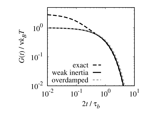
Figure 1:

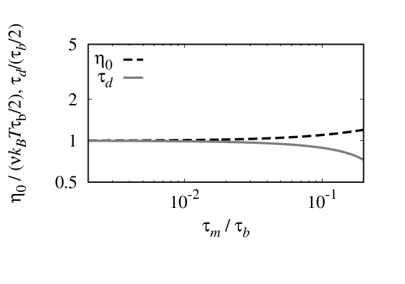
Figure 2:

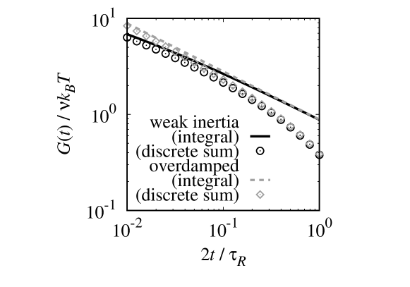
Figure 3:

References

- [1] Doi M, Edwards SF, “The Theory of Polymer Dynamics”, (1986), Oxford University Press, Oxford.
- [2] van Kampen NG, “Stochastic Processes in Physics and Chemistry”, 3rd ed, (2007), Elsevier, Amsterdam.
- [3] Sekimoto K, J Phys Soc Jpn, 68, 1448 (1999).
- [4] Matsuo M, Sasa S, Physica A, 276, 188 (2000).
- [5] Öttinger HC, “Stochastic Processes in Polymeric Fluids: Tools and Examples for Developing Simulation Algorithms”, (1996), Springer, Berlin.
- [6] Kröger M, Phys Rep, 390, 453 (2004).
- [7] Booij HC, J Rheol, 32, 47 (1988).
- [8] Grassia P, Hinch EJ, J Fluid Mech, 308, 255 (1996).
- [9] Schieber JD, Öttinger HC, J Chem Phys, 89, 6972 (1998).
- [10] Degond P, Liu H, Netw Heterog Media, 4, 625 (2009).
- [11] Wuttke J, arXiv:1103.4238.
- [12] Gardiner CW, Handbook of Stochastic Methods (Springer, Berlin, 2004), 3rd ed.
- [13] Evans DJ, Morris GP, “Statistical Mechanics of Nonequilibrium Liquids”, 2nd ed., (2008), Cambridge University Press, Cambridge.
- [14] Kremer K, Grest GS, J Chem Phys, 92, 5057 (1990).
- [15] Olver FWJ, Lozier DW, Boisvert RF, Clark CW eds., “NIST Handbook of Mathematical Functions”, (2010), Cambridge University Press, New York.
- [16] Likhtman AE, Sukumaran SK, Ramirez J, Macromolecules, 40, 6748 (2007).
- [17] Masubuchi Y, Takata H, Amamoto Y, Yamamoto T, Nihon Reoroji Gakkaishi (J Soc Rheol Jpn), 46, 171 (2018).
- [18] Uneyama T, Miyaguchi T, Akimoto T, Phys Rev E, 99, 032127 (2019).
- [19] Kawasaki K, J Phys A: Math Nucl Gen, 6, 1289 (1973).
- [20] Fox RF, J Math Phys, 18, 2331 (1977).
- [21] Bateman H, “Tables of Integral Transforms”, vol. 1, (1954), McGraw-Hill, New York.