Polynomial Tensor Sketch for Element-wise Function of Low-Rank Matrix

Supplementary Material:
Polynomial Tensor Sketch for Element-wise Function of Low-Rank Matrix

Abstract

This paper studies how to sketch element-wise functions of low-rank matrices. Formally, given low-rank matrix $A=[A_{ij}]$ and scalar non-linear function $f$, we aim for finding an approximated low-rank representation of the (possibly high-rank) matrix $[f(A_{ij})]$. To this end, we propose an efficient sketching-based algorithm whose complexity is significantly lower than the number of entries of $A$, i.e., it runs without accessing all entries of $[f(A_{ij})]$ explicitly. The main idea underlying our method is to combine a polynomial approximation of $f$ with the existing tensor sketch scheme for approximating monomials of entries of $A$. To balance the errors of the two approximation components in an optimal manner, we propose a novel regression formula to find polynomial coefficients given $A$ and $f$. In particular, we utilize a coreset-based regression with a rigorous approximation guarantee. Finally, we demonstrate the applicability and superiority of the proposed scheme under various machine learning tasks.

1 Introduction

Given a low-rank matrix $A=[A_{ij}]\in\mathbb{R}^{n\times n}$ with $A=UV^{\top}$ for some matrices $U,V\in\mathbb{R}^{n\times d}$ with $d\ll n$ and a scalar non-linear function $f:\mathbb{R}\rightarrow\mathbb{R}$, we are interested in the following element-wise matrix function:

$$f^{\odot}({A})\in\mathbb{R}^{n\times n},\quad\text{where }\ f^{\odot}({A})_{ij}:=\left[f(A_{ij})\right].$$

Our goal is to design a fast algorithm for computing tall-and-thin matrices $T_{U},T_{V}$ in time $o(n^{2})$such that $f^{\odot}({A})\approx T_{U}T_{V}^{\top}$. In particular, our algorithm should run without computing all entries of $A$ or $f^{\odot}({A})$ explicitly. As an side, we obtain a $o(n^{2})$-time approximation scheme of $f^{\odot}({A})\boldsymbol{x}\approx T_{U}T_{V}^{\top}\boldsymbol{x}$ for an arbitrary vector $\boldsymbol{x}\in\mathbb{R}^{n}$ due to the associative property of matrix multiplication, where the exact computation of $f^{\odot}({A})\boldsymbol{x}$ requires the complexity of $\Theta(n^{2})$.

The matrix-vector multiplication $f^{\odot}({A})\boldsymbol{x}$ or the low-rank decomposition $f^{\odot}({A})\approx T_{U}T_{V}^{\top}$ is useful in many machine learning algorithms. For example, the Gram matrices of certain kernel functions, e.g., polynomial and radial basis function (RBF), are element-wise matrix functions where the rank is the dimension of the underlying data. Such matrices are the cornerstone of so-called kernel methods and the ability to multiply the Gram matrix to a vector suffices for most kernel learning. The Sinkhorn-Knopp algorithm is a powerful, yet simple, tool for computing optimal transport distances (Cuturi, 2013; Altschuler et al., 2017) and also involves the matrix-vector multiplication $f^{\odot}({A})\boldsymbol{x}$ with $f(x)=\exp(x)$. Finally, $f^{\odot}({UV^{\top}})$ can also describe the non-linear computation of activation in a layer of deep neural networks (Goodfellow et al., 2016), where $U$, $V$ and $f$ correspond to input, weight and activation function (e.g., sigmoid or ReLU) of the previous layer, respectively.

Unlike the element-wise matrix function $f^{\odot}({A})$, a traditional matrix function $f(A)$ is defined on their eigenvalues (Higham, 2008) and possesses clean algebraic properties, i.e., it preserves eigenvectors. For example, given a diagonalizable matrix $A=PDP^{-1}$, it is defined that $f(A)=Pf^{\odot}(D)P^{-1}$. A classical problem addressed in the literature is of approximating the trace of $f(A)$ (or $f(A)\boldsymbol{x}$) efficiently (Han et al., 2017; Ubaru et al., 2017). However, these methods are not applicable to our problem because element-wise matrix functions are fundamentally different from the traditional function of matrices, e.g., they do not guarantee the spectral property. We are unaware of any approximation algorithm that targets general element-wise matrix functions. The special case of element-wise kernel functions such as $f(x)=\exp(x)$ and $f(x)=x^{k}$, as been address in the literature, e.g., using random Fourier features (RFF) (Rahimi & Recht, 2008; Pennington et al., 2015), Nyström method (Williams & Seeger, 2001), sparse greedy approximation (Smola & Schökopf, 2000) and sketch-based methods (Pham & Pagh, 2013; Avron et al., 2014; Meister et al., 2019; Ahle et al., 2020), just to name a few examples. We aim for not only designing an approximation framework for general $f$, but also outperforming the previous approximations (e.g., RFF) even for the special case $f(x)=\exp(x)$.

The high-level idea underlying our method is to combine two approximation schemes: TensorSketch approximating the element-wise matrix function of monomial $x^{k}$ and a degree-$r$ polynomial approximation $p_{r}(x)=\sum_{j=0}^{r}c_{j}x^{j}$ of function $f$, e.g., $f(x)=\exp(x)\approx p_{r}(x)=\sum_{j=0}^{r}\frac{1}{j!}x^{j}$. More formally, we consider the following approximation:

$$f^{\odot}({A}) ~{}\overset{\text{(a)}}{\approx}~{}\sum_{j=0}^{r}c_{j}\cdot(x^{j})^{\odot}(A)$$

$$~{}\overset{\text{(b)}}{\approx}~{}\sum_{j=0}^{r}c_{j}\cdot\text{{\sc TensorSketch }}\left((x^{j})^{\odot}(A)\right),$$

which we call Poly-TensorSketch. This is a linear-time approximation scheme with respect to $n$ under the choice of $r=\mathcal{O}(1)$. Here, a non-trivial challenge occurs: a larger degree $r$ is required to approximate an arbitrary function $f$ better, while the approximation error of TensorSketch is known to increase exponentially with respect to $r$ (Pham & Pagh, 2013; Avron et al., 2014). Hence, it is important to choose good $c_{j}$’s for balancing two approximation errors in both (a) and (b). The known (truncated) polynomial expansions such as Taylor or Chebyshev (Mason & Handscomb, 2002) are far from being optimal for this purpose (see Section 3.2 and 4.1 for more details).

To address this challenge, we formulate an optimization problem on the polynomial coefficients (the $c_{j}$s) by relating them to the approximation error of Poly-TensorSketch. However, this optimization problem is intractable since the objective involves an expectation taken over random variables whose supports are exponentially large. Thus, we derive a novel tractable alternative optimization problem based on an upper bound the approximation error of Poly-TensorSketch. This problem turns out to be an instance of generalized ridge regression (Hemmerle, 1975), and as such has a closed-form solution. Furthermore, we observe that the regularization term effectively forces the coefficients to be exponentially decaying, and this compensates the exponentially growing errors of TensorSketch with respect to the rank, while simultaneously maintaining a good polynomial approximation to the scalar function $f$ given entries of $A$. We further reduce its complexity by regressing only a subset of the matrix entries found by an efficient coreset clustering algorithm (Har-Peledx, 2008): if matrix entries are close to the selected coreset, then the resulting coefficient is provably close to the optimal one. Finally, we construct the regression with respect to Chebyshev polynomial basis (instead of monomials), i.e., $p_{r}(x)=\sum_{j=0}^{r}{c}_{j}t_{j}(x)$ for the Chebyshev polynomial $t_{j}(x)$ of degree $j$, in order to resolve numerical issues arising for large degrees.

We evaluate the approximation quality of our algorithm under the RBF kernels of synthetic and real-world datasets. Then, we apply the proposed method to classification using kernel SVM (Cristianini et al., 2000; Scholkopf & Smola, 2001) and computation of optimal transport distances (Cuturi, 2013) which require to compute element-wise matrix functions with $f(x)=\exp(x)$. Our experimental results confirm that our scheme is at the order of magnitude faster than the exact method with a marginal loss on accuracy. Furthermore, our scheme also significantly outperforms a state-of-the-art approximation method, RFF for the aforementioned applications. Finally, we demonstrate a wide applicability of our method by applying it to the linearization of neural networks, which requires to compute element-wise matrix functions with $f(x)=\mathtt{sigmoid}(x)$.

2 Preliminaries

In this section, we provide backgrounds on the randomized sketching algorithms CountSketch and TensorSketch that are crucial components of the proposed scheme.

First, CountSketch (Charikar et al., 2002; Weinberger et al., 2009) was proposed for an effective dimensionality reduction of high-dimensional vector $\boldsymbol{u}\in\mathbb{R}^{d}$. Formally, consider a random hash function $h:[d]\rightarrow[m]$ and a random sign function $s:[d]\rightarrow\{-1,+1\}$, where $[d]:=\{1,\dots,d\}$. Then, CountSketch transforms $\boldsymbol{u}$ into $C_{\boldsymbol{u}}\in\mathbb{R}^{m}$ such that $[C_{\boldsymbol{u}}]_{j}:=\sum_{i:h(i)=j}s(i){u}_{i}$ for $j\in[m]$. The algorithm takes $\mathcal{O}(d)$ time to run since it requires a single pass over the input. It is known that applying the same CountSketch transform on two vectors preserves the dot-product, i.e., $\left\langle{\boldsymbol{u},\boldsymbol{v}}\right\rangle=\mathbf{E}\left[\left\langle{C_{\boldsymbol{u}},C_{\boldsymbol{v}}}\right\rangle\right]$.

TensorSketch (Pham & Pagh, 2013) was proposed as a generalization of CountSketch to tensor products of vectors. Given $\boldsymbol{u}\in\mathbb{R}^{d}$ and a degree $k$, consider i.i.d. random hash functions $h_{1},\dots,h_{k}:[d]\rightarrow[m]$ and i.i.d. random sign functions $s_{1},\dots,s_{k}:[d]\rightarrow\{-1,+1\}$, TensorSketch applied to $\boldsymbol{u}$ is defined as the $m$-dimensional vector $T_{\boldsymbol{u}}\in\mathbb{R}^{m}$ such that $j\in[m]$,

$$[T_{\boldsymbol{u}}^{(k)}]_{j}:=\sum_{H(i_{1},\dots,i_{k})=j}s_{1}(i_{1})\dots s_{k}(i_{k}){u}_{i_{1}}\dots u_{i_{k}},$$

where $H(i_{1},\dots,i_{k})\equiv h_{1}(i_{1})+\dots+h_{k}(i_{k})\ \ \text{(mod }\ m).$ In (Pham & Pagh, 2013; Avron et al., 2014; Pennington et al., 2015; Meister et al., 2019), TensorSketch was used for approximating of the power of dot-product between vectors. In other words, let $T_{\boldsymbol{u}}^{(k)},T_{\boldsymbol{v}}^{(k)}$ be the same TensorSketch on $\boldsymbol{u},\boldsymbol{v}\in\mathbb{R}^{d}$ with degree $k$. Then, it holds that

$$\left\langle{\boldsymbol{u},\boldsymbol{v}}\right\rangle^{k}=\left\langle{\boldsymbol{u}^{\otimes k},\boldsymbol{v}^{\otimes k}}\right\rangle=\mathbf{E}\left[\left\langle{T_{\boldsymbol{u}}^{(k)},T_{\boldsymbol{v}}^{(k)}}\right\rangle\right],$$

where $\otimes$ denotes the tensor product (or outer-product) and $\boldsymbol{u}^{\otimes k}:=\boldsymbol{u}\otimes\dots\otimes\boldsymbol{u}\in\mathbb{R}^{d^{k}}$ ($k-1$ times). This can be naturally extended to matrices $U,V\in\mathbb{R}^{n\times d}$. Suppose $T_{U}^{(k)},T_{V}^{(k)}\in\mathbb{R}^{n\times m}$ are the same TensorSketch on each row of $U,V$, and it follows that $(UV^{\top})^{\odot k}=\mathbf{E}\left[T_{U}^{(k)}T_{V}^{(k)\top}\right]$ where $A^{\odot k}:=[A^{k}_{ij}]$. Pham & Pagh (2013) devised a fast way to compute TensorSketch using the Fast Fourier Transform (FFT) as described in Algorithm 1.

Algorithm 1 TensorSketch (Pham & Pagh, 2013)

1:  Input: $U\in\mathbb{R}^{n\times d}$, degree $k$, sketch dimension $m$

2:  Draw $k$ i.i.d. random hash functions $h_{1},\dots,h_{k}:[d]\rightarrow[m]$

3:  Draw $k$ i.i.d. random sign functions $s_{1},\dots,s_{k}:[d]\rightarrow\{+1,-1\}$

4:  $C_{U}^{(i)}$ $\leftarrow$ CountSketch on each row of $U$ using $h_{i}$ and $s_{i}$ for $i=1,\dots,k$.

5:  $T_{U}^{(k)}\leftarrow\text{\sc FFT}^{-1}\left(\text{\sc FFT}(C_{U}^{(1)})\odot\cdots\odot\text{\sc FFT}(C_{U}^{(k)})\right)$

6:  Output : $T_{U}^{(k)}$

In Algorithm 1, $\odot$ is the element-wise multiplication (also called the Hadamard product) between two matrices of the same dimension and $\text{\sc FFT}(C),\text{\sc FFT}^{-1}(C)$ are the Fast Fourier Transform and its inverse applied to each row of a matrix $C\in\mathbb{R}^{n\times m}$, respectively. The cost of the FFTs is $\mathcal{O}(nm\log m)$ and so the total cost of Algorithm 1 is $\mathcal{O}(nk(d+m\log m))$ time since it runs FFT and CountSketch $k$ times. Avron et al. (2014) proved a tight bound on the variance (or error) of TensorSketch as follows.

Theorem 1 (Avron et al. (2014))

Given $U,V\in\mathbb{R}^{n\times d}$, let $T_{U}^{(k)},T_{V}^{(k)}\in\mathbb{R}^{n\times m}$ be the same TensorSketch of $U,V$ with degree $k\geq 0$ and sketch dimension $m$. Then, it holds

$$\mathbf{E}\left[\left\|\left(UV^{\top}\right)^{\odot k}-T_{U}^{(k)}{T_{V}^{(k)}}^{\top}\right\|_{F}^{2}\right]$$

$$\leq\frac{(2+3^{k})\left(\sum_{i}(\sum_{j}U_{ij}^{2})^{k}\right)\left(\sum_{i}(\sum_{j}V_{ij}^{2})^{k}\right)}{m}.$$ (2.1)

The above theorem implies the error of TensorSketch becomes small for large sketch dimension $m$, but can grow fast with respect to degree $k$. Recently, Ahle et al. (2020) proposed another method whose error bound is tighter with respect to $k$, but can be worse with respect to another factor so-called statistical dimension (Avron et al., 2017).

3 Linear-time Approximation of Element-wise Matrix Functions

Given a scalar function $f:\mathbb{R}\rightarrow\mathbb{R}$ and matrices $U,V\in\mathbb{R}^{n\times d}$ with $d\ll n$, our goal is to design an efficient algorithm to find $T_{U},T_{V}\in\mathbb{R}^{n\times d^{\prime}}$ with $d^{\prime}\ll n$ in $o(n^{2})$ time such that

$$f^{\odot}(UV^{\top})\approx T_{U}T_{V}^{\top}\in\mathbb{R}^{n\times n}.$$

Namely, we aim for finding a low-rank approximation of $f^{\odot}(UV^{\top})$ without computing all $n^{2}$ entries of $UV^{\top}$. We first describe the proposed approximation scheme in Section 3.1 and provide further ideas for minimizing the approximation gap in Section 3.2.

Algorithm 2 Poly-TensorSketch

1:  Input:  $U,V\in\mathbb{R}^{n\times d}$, degree $r$, coefficient $c_{0},\dots,c_{r}$, sketch dimension $m$

2:  Draw $r$ i.i.d. random hash functions $h_{1},\dots,h_{r}:[d]\rightarrow[m]$

3:  Draw $r$ i.i.d. random sign functions $s_{1},\dots,s_{r}:[d]\rightarrow\{+1,-1\}$

4:  $T_{U}^{(1)},T_{V}^{(1)}\leftarrow$ CountSketch of $U,V$ using $h_{1}$ and $s_{1}$, respectively.

5:  $F_{U},F_{V}\leftarrow$ ${\textsc{FFT}}(T_{U}^{(1)})$,  ${\textsc{FFT}}(T_{V}^{(1)})$

6:  $\Gamma\leftarrow c_{0}T_{U}^{(0)}T_{V}^{(0)\top}+c_{1}T_{U}^{(1)}T_{V}^{(1)\top}$

7:  for $j=2$ to $r$ do

8:     $C_{U},C_{V}\leftarrow$ CountSketch of $U,V$ using $h_{j}$ and $s_{j}$, respectively.

9:     $F_{U},F_{V}\leftarrow{\textsc{FFT}}(C_{U})\odot F_{U},\ {\textsc{FFT}}(C_{V})\odot F_{V}$

10:     $T_{U}^{(j)},T_{V}^{(j)}\leftarrow{\textsc{FFT}}^{-1}\left(F_{U}\right),\ {\textsc{FFT}}^{-1}\left(F_{V}\right)$

11:     $\Gamma\leftarrow\Gamma+c_{j}T_{U}^{(j)}{T_{V}^{(j)\top}}$

12:  end for

13:  Output : $\Gamma$

3.1 Poly-TensorSketch Transform

Suppose we have a polynomial $p_{r}(x)=\sum_{j=0}^{r}c_{j}x^{j}$ approximating $f(x)$, e.g., $f(x)=\exp(x)$ and its (truncated) Taylor series $p_{r}(x)=\sum_{j=0}^{r}\frac{1}{j!}x^{j}$. Then, we consider the following approximation scheme, coined Poly-TensorSketch :

$$f^{\odot}({UV^{\top}}) ~{}\overset{\text{(a)}}{\approx}~{}\sum_{j=0}^{r}c_{j}(UV^{\top})^{\odot j}~{}\overset{\text{(b)}}{\approx}~{}\sum_{j=0}^{r}c_{j}T_{U}^{(j)}T_{V}^{(j)\top},$$ (3.1)

where $T_{U}^{(j)},T_{V}^{(j)}\in\mathbb{R}^{n\times m}$ are the same TensorSketch of $U,V$ with degree $j$ and sketch dimension $m$, respectively. Namely, our main idea is to combine (a) a polynomial approximation of a scalar function with (b) the randomized tensor sketch of a matrix. Instead of running Algorithm 1 independently for each $j\in[r]$, we utilize the following recursive relation to amortize operations:

$$T_{U}^{(j)}={\textsc{FFT}}^{-1}\left({\textsc{FFT}}(C_{U})\odot{\textsc{FFT}}(T_{U}^{(j-1)})\right),$$

where $C_{U}$ is the CountSketch on each row of $U$ whose randomness is independently drawn from that of $T_{U}^{(j-1)}$. Since each recursive step can be computed in $\mathcal{O}(n(d+m\log m))$ time, computing all $T_{U}^{(j)}$ for $j\in[r]$ requires $\mathcal{O}(nr(d+m\log m))$ operations. Hence, the overall complexity of Poly-TensorSketch, formally described in Algorithm 2, is $\mathcal{O}(n)$ if $r,d,m=\mathcal{O}(1)$.

Observe that multiplication of $\Gamma$ (i.e., the output of Algorithm 2) and an arbitrary vector $\boldsymbol{x}\in\mathbb{R}^{d}$ can be done in $\mathcal{O}(nmr)$ time due to $\Gamma\boldsymbol{x}=\sum_{j=0}^{r}c_{j}T_{U}^{(j)}T_{V}^{(j)\top}\boldsymbol{x}$. Hence, for $r,m,d=\mathcal{O}(1)$, Poly-TensorSketch can approximate $f^{\odot}(UV^{\top})\boldsymbol{x}$ in $\mathcal{O}(nr(d+m\log m))=\mathcal{O}(n)$ time. As for the error, we prove the following error bound.

Proposition 2

Given $U,V\in\mathbb{R}^{n\times d}$, $f:\mathbb{R}\rightarrow\mathbb{R}$, suppose that $|f(x)-\sum_{j=0}^{r}c_{j}x^{j}|\leq\varepsilon$ in a closed interval containing all entries of $UV^{\top}$ for some $\varepsilon>0$. Then, it holds that

$$\mathbf{E}\left[\left\|f^{\odot}(UV^{\top})-\Gamma\right\|_{F}^{2}\right]\leq 2n^{2}\varepsilon^{2}$$

$$+\sum_{j=1}^{r}\frac{2rc_{j}^{2}(2+3^{j})\left(\sum_{i}(\sum_{k}U_{ik}^{2})^{j}\right)\left(\sum_{i}(\sum_{k}V_{ik}^{2})^{j}\right)}{m},$$ (3.2)

where $\Gamma$ is the output of Algorithm 2.

The proof of Proposition 2 is given in the supplementary material. Note that even when $\varepsilon$ is close to $0$, the error bound (2) may increase exponentially with respect to the degree $r$. This is because the approximation error of TensorSketch grows exponentially with respect to the degree (see Theorem 1). Therefore, in order to compensate, it is desirable to use exponentially decaying (or even truncated) coefficient $\{c_{j}\}$. However, we are now faced with the challenge of finding exponentially decaying coefficients, while not hurting the approximation quality of $f$. Namely, we want to balance the two approximation components of Poly-TensorSketch: TensorSketch and a polynomial approximation for $f$. In the following section, we propose a novel approach to find the optimal coefficients minimizing the approximation error of Poly-TensorSketch.

3.2 Optimal Coefficient via Ridge Regression

A natural choice for the coefficients is to utilize a polynomial series such as Taylor, Chebyshev (Mason & Handscomb, 2002) or other orthogonal basis expansions (see Szego (1939)). However, constructing the coefficient in this way focuses on the error of the polynomial approximation of $f$, and ignores the error of TensorSketch which depends on the decay of the coefficient, as reflected in the error bound (2). To address the issue, we study the following optimization to find the optimal coefficient:

$$\min_{\boldsymbol{c}\in\mathbb{R}^{r+1}}\mathbf{E}\left[\left\lVert f^{\odot}(UV^{\top})-\Gamma\right\rVert_{F}^{2}\right],$$ (3.3)

where $\Gamma$ is the output of Poly-TensorSketch and $\boldsymbol{c}=[c_{0},\dots,c_{r}]$ is a vector of the coefficient. However, it is not easy to solve the above optimization directly as its objective involves an expectation over random variables with a huge support, i.e., uniform hash and binary sign functions. Instead, we aim for minimizing an upper bound of the approximation error (3.3). To this end, we define the following notation.

Definition 3

Let $X\in\mathbb{R}^{n^{2}\times(r+1)}$ be the matrix whose $k$-th column corresponds to the vectorization of $(UV^{\top})_{ij}^{k-1}$ for all $i,j\in[n]$, $\boldsymbol{f}\in\mathbb{R}^{n^{2}}$ be the vectorization of $f^{\odot}({UV^{\top}})$ and $W\in\mathbb{R}^{(r+1)\times(r+1)}$ be a diagonal matrix such that $W_{11}=0$ and for $i=2,\dots,r+1$

$$W_{ii}=\sqrt{\frac{r(2+3^{i})(\sum_{j}(\sum_{k}U_{jk}^{2})^{i})(\sum_{j}(\sum_{k}V_{jk}^{2})^{i})}{m}}.$$

Using the above notation, we establish the following error bound.

Lemma 4

Given $U,V\in\mathbb{R}^{n\times d}$ and $f:\mathbb{R}\rightarrow\mathbb{R}$, consider $X,\boldsymbol{f}$ and $W$ defined in Definition 3. Then, it holds

$$\mathbf{E}\left[\left\lVert f^{\odot}(UV^{\top})-\Gamma\right\rVert_{F}^{2}\right]\leq 2\|X\boldsymbol{c}-\boldsymbol{f}\|_{2}^{2}+2\|W\boldsymbol{c}\|_{2}^{2},$$ (3.4)

where $\Gamma$ is the output of Algorithm 2.

The proof of Lemma 4 is given in the supplementary material. Observe that the error bound (3.4) is a quadratic form of $\boldsymbol{c}\in\mathbb{R}^{r+1}$, where it is straightforward to obtain a closed-form solution for minimizing (3.4):

$$\boldsymbol{c}^{*} :=\operatorname*{arg\,min}_{\boldsymbol{c}\in\mathbb{R}^{r+1}}\|X\boldsymbol{c}-\boldsymbol{f}\|_{2}^{2}+\|W\boldsymbol{c}\|_{2}^{2}$$

$$=\left(X^{\top}X+W^{2}\right)^{-1}X^{\top}\boldsymbol{f}.$$ (3.5)

This optimization task is also known as generalized ridge regression (Hemmerle, 1975). The solution (3.2) minimizes the regression error (i.e., the error of polynomial), while it is regularized by $W$, i.e., $W_{ii}$ is a regularizer of $c_{i}$. Namely, if $W_{ii}$ grows exponentially with respect to $i$, then $c_{i}^{*}$ may decay exponentially (this compensates the error of TensorSketch with degree $i$). By substituting $\boldsymbol{c}^{*}$ into the error bound (3.4), we obtain the following multiplicative error bound of Poly-TensorSketch.

Theorem 5

Given $U,V\in\mathbb{R}^{n\times d}$ and $f:\mathbb{R}\rightarrow\mathbb{R}$, consider $X$ defined in Definition 3. Then, it holds

$$\mathbf{E}\left[\left\lVert f^{\odot}(UV^{\top})-\Gamma\right\rVert_{F}^{2}\right]\leq\left(\frac{2}{1+\frac{m{\sigma}^{2}}{rC}}\right)\|f^{\odot}(UV^{\top})\|_{F}^{2},$$ (3.6)

where $\Gamma$ is the output of Algorithm 2 with the coefficient $\boldsymbol{c}^{*}$ in (3.2), $\sigma\geq 0$ is the smallest singular value of $X$ and $C=\max(5\|U\|_{F}^{2}\|V\|_{F}^{2},(2+3^{r})(\sum_{j}(\sum_{k}U_{jk}^{2})^{r})(\sum_{j}(\sum_{k}V_{jk}^{2})^{r}))$.

The proof of Theorem 5 is given in the supplementary material. Observe that the error bound (3.6) is bounded by 2$\|f^{\odot}(UV^{\top})\|_{F}^{2}$ since $m,r,\sigma,C\geq 0$. On the other hand, we recall that the error bound (2), i.e., Poly-TensorSketch without using the optimal coefficient $\boldsymbol{c}^{*}$, can grow exponentially with respect to $r$. We indeed observe that $\boldsymbol{c}^{*}$ is empirically superior to the coefficient of the popular Taylor and Chebyshev series expansions with respect to the error of Poly-TensorSketch (see Section 4.1 for more details). We also remark that the error bound (3.6) of Poly-TensorSketch is even better than that (1) of TensorSketch even for the case of monomial $f(x)=x^{k}$. This is primarily because the former is achievable by paying an additional cost for computing the optimal coefficient vector (3.2). In what follows, we discuss the extra cost.

3.3 Reducing Complexity via Coreset Regression

To obtain the optimal coefficient $\boldsymbol{c}^{*}$ in (3.2), one can check that $\mathcal{O}(r^{2}n^{2}+r^{3})$ operations are required because of computing $X^{\top}X$ for $X\in\mathbb{R}^{n^{2}\times(r+1)}$ (see Definition 3). This hurts the overall complexity of Poly-TensorSketch. Instead, we choose a subset of entries in $UV^{\top}$ and approximately find the coefficient $\boldsymbol{c}^{*}$ based on the selected entries.

Algorithm 3 Greedy $k$-center

1:  Input: $\boldsymbol{u}_{1},\dots,\boldsymbol{u}_{n}\in\mathbb{R}^{d}$, number of clusters $k$

2:  $a\leftarrow$ uniformly random in $\{1,2,\dots,n\}$ and $S\leftarrow\{a\}$

3:  $\Delta_{i}\leftarrow\left\lVert\boldsymbol{u}_{i}-\boldsymbol{u}_{a}\right\rVert_{2}$ for all $i\in[n]$

4:  for $i=2$ to $k$  do

5:     $a\leftarrow\arg\max_{i}\Delta_{i}$ and $S\leftarrow S\cup\{a\}$

6:     $\Delta_{i}\leftarrow\min(\Delta_{i},\left\lVert\boldsymbol{u}_{i}-\boldsymbol{u}_{a}\right\rVert_{2})$ for all $i$

7:  end for

8:  $P(i)\leftarrow\arg\min_{j\in S}\left\lVert\boldsymbol{u}_{i}-\boldsymbol{u}_{j}\right\rVert_{2}$ for all $i$

9:  Output: $\{\boldsymbol{u}_{i}:i\in S\},\ P$

Algorithm 4 Coefficient approximation via coreset

1:  Input:  $U,V\in\mathbb{R}^{n\times d}$, a function $f$, number of clusters $k$, degree $r$

2:  $\{\overline{\boldsymbol{u}}_{i}\}_{i=1}^{k},P_{1}\leftarrow$ Algorithm 3 with rows in $U$ and $k$

3:  $\{\overline{\boldsymbol{v}}_{i}\}_{i=1}^{k},P_{2}\leftarrow$ Algorithm 3 with rows in $V$ and $k$

4:  $\varepsilon_{U}\leftarrow\sum_{i}\left\lVert\boldsymbol{u}_{i}-\overline{\boldsymbol{u}}_{P_{1}(i)}\right\rVert_{2}$, $\varepsilon_{V}\leftarrow\sum_{i}\left\lVert\boldsymbol{v}_{i}-\overline{\boldsymbol{v}}_{P_{2}(i)}\right\rVert_{2}$

5:  if $\varepsilon_{U}\sum_{i}\left\lVert\boldsymbol{v}_{i}\right\rVert_{2}<\varepsilon_{V}\sum_{j}\left\lVert\boldsymbol{u}_{j}\right\rVert_{2}$ then

6:     $\overline{X},D$ and $\overline{\boldsymbol{f}}\leftarrow$ matrices and vector defined in Definition 6 with $\overline{U},V$ and $P_{1}$

7:  else

8:     $\overline{X},D$ and $\overline{\boldsymbol{f}}\leftarrow$ matrices and vector defined in Definition 6 with $U,\overline{V}$ and $P_{2}$

9:  end if

10:  Output : $\left(\overline{X}^{\top}D\overline{X}+W^{2}\right)^{-1}\overline{X}^{\top}D\overline{\boldsymbol{f}}$

More formally, suppose $\overline{U}\in\mathbb{R}^{k\times d}$ is a matrix containing certain $k$ rows of $U\in\mathbb{R}^{n\times d}$ and we use the following approximation:

$$\boldsymbol{c}^{*} =\left(X^{\top}X+W^{2}\right)^{-1}X^{\top}\boldsymbol{f}$$

$$\approx\left(\overline{X}^{\top}D\overline{X}+W^{2}\right)^{-1}\overline{X}^{\top}D\overline{\boldsymbol{f}},$$ (3.7)

where $\overline{X},D$ and $\overline{\boldsymbol{f}}$ are defined as follows.

Definition 6

Let $\overline{X}\in\mathbb{R}^{kn\times(r+1)}$ be the matrix whose $\ell$-th column is the vectorization of $(\overline{U}V^{\top})_{ij}^{\ell-1}$ for $i\in[k],j\in[n]$ and $\overline{\boldsymbol{f}}\in\mathbb{R}^{kn}$ be the vectorization of $f^{\odot}(\overline{U}V^{\top})$. Given a mapping $P:[n]\rightarrow[k]$, let $D\in\mathbb{R}^{kn\times kn}$ be a diagonal matrix where $D_{ii}=\left|\{s:P(s)=\lceil i/n\rceil\}\right|$.

Computing (3.3) requires $\mathcal{O}(r^{2}kn+r^{3})=\mathcal{O}(n)$ for $r,k=\mathcal{O}(1)$. In what follows, we show that if rows of $U$ are close to those of $\overline{U}$ under the mapping $P$, then the approximation (3.3) becomes tighter. To this end, we say $\overline{U}$ is a $\varepsilon$-coreset of $U$ for some $\varepsilon>0$ if there exists a mapping $P:[n]\rightarrow[k]$ such that $\sum_{i=1}^{n}\left\lVert\boldsymbol{u}_{i}-\overline{\boldsymbol{u}}_{P(i)}\right\rVert_{2}\leq\varepsilon,$ where $\boldsymbol{u}_{i},\overline{\boldsymbol{u}}_{i}$ are the $i$-th rows of $U,\overline{U}$, respectively. Using the notation, we now present the following error bound of Poly-TensorSketch under the approximated coefficient vector in (3.3).

Theorem 7

Given $U,V\in\mathbb{R}^{n\times d}$ and $f:\mathbb{R}\rightarrow\mathbb{R}$, consider $\varepsilon$-coreset $\overline{U}\in\mathbb{R}^{k\times d}$ of $U$ with $\overline{X},D,\overline{\boldsymbol{f}}$ and $P$ defined in Definition 6. For the approximated coefficient vector $\boldsymbol{c}$ in (3.3), assume that $(f(x)-\sum_{j=0}^{r}c_{j}x^{j})^{2}$ is a $L$-Lipschitz function. Then, it holds

$$\mathbf{E}\left[\left\lVert f^{\odot}(UV^{\top})-\Gamma\right\rVert_{2}^{2}\right]$$

$$\leq\frac{2}{\left(1+\frac{m\overline{\sigma}^{2}}{r{C}}\right)}\left\lVert\overline{\boldsymbol{f}}\right\rVert_{2}^{2}+2\varepsilon L\left(\sum_{i=1}^{n}\left\lVert\boldsymbol{v}_{i}\right\rVert_{2}\right),$$ (3.8)

where $\Gamma$ is the output of Algorithm 2 with $\boldsymbol{c}$, $\boldsymbol{v}_{i}$ is the $i$-th row of $V$, $\overline{\sigma}$ is the smallest singular value of $D^{1/2}\overline{X}$ and ${C}:=\max(5\|{U}\|_{F}^{2}\|V\|_{F}^{2},(2+3^{r})(\sum_{j}(\sum_{k}{U}_{jk}^{2})^{r})(\sum_{j}(\sum_{k}V_{jk}^{2})^{r}))$.

The proof of Theorem 7 is given in the supplementary material. Observe that when $\varepsilon$ is small, the error bound (7) becomes closer to that under the optimal coefficient (3.6). To find a coreset with small $\varepsilon$, we use the greedy $k$-center algorithm (Har-Peledx, 2008) described in Algorithm 3. We remark that the greedy $k$-center runs in $\mathcal{O}(ndk)$ time and it marginally increases the overall complexity of Poly-TensorSketch in our experiments. Moreover, we indeed observe that various real-world datasets used in our experiments are well-clustered, which leads to a small $\varepsilon$ (see supplementary material for details).

Algorithm 4 summarizes the proposed scheme for computing the approximated coefficient vector $\boldsymbol{c}$ in (3.3) with the greedy $k$-center algorithm. Here, we run the greedy $k$-center on both rows in $U$ and $V$, and choose the one with a smaller value in the second term in (7), i.e., $\varepsilon_{U}\sum_{i}\left\lVert\boldsymbol{v}_{i}\right\rVert_{2}$ or $\varepsilon_{V}\sum_{i}\left\lVert\boldsymbol{u}_{i}\right\rVert_{2}$ (see also line 4-8 in Algorithm 4). We remark that Algorithm 4 requires $\mathcal{O}(nk(d+r^{2})+r^{3})$ operations, hence, applying this to Poly-TensorSketch results in $\mathcal{O}(nk(d+r^{2})+r^{3})+\mathcal{O}(nr(d+m\log m))$ time in total. If one chooses $m,k,r=\mathcal{O}(1)$, the overall running time becomes $\mathcal{O}(nd)$ which is linear in the size of input matrix. For example, we choose $r,k,m=10$ in our experiments.

Chebyshev polynomial regression for avoiding a numerical issue. Recall that $X$ contains $(UV^{\top})_{ij}^{r}$ (see Definition 3). If entries in $UV^{\top}$ are greater (or smaller) than $1$ and degree $r$ is large, $X$ can have huge (or negligible) values. This can cause a numerical issue for computing the optimal coefficient (3.2) (or (3.3)) using $X$. To alleviate the issue, we suggest to construct a matrix $X^{\prime}\in\mathbb{R}^{n^{2}\times(r+1)}$ whose entries are the output of the Chebyshev polynomials: $(X^{\prime})_{ij}=t_{j}((UV^{\top})_{k\ell})$ where $k,\ell\in[n]$ corresponds to index $i\in[n^{2}]$, $j\in[r+1]$ and $t_{j}(x)$ is the Chebyshev polynomial of degree $j$ (Mason & Handscomb, 2002). Now, the value of $t_{j}(x)$ is always in $[-1,1]$ and does not monotonically increase or decrease with respect to the degree $j$. Then, we find the optimal coefficient $\boldsymbol{c}^{\prime}\in\mathbb{R}^{r+1}$ based on Chebyshev polynomials as follows:

$${\boldsymbol{c}^{\prime}}=\left({X^{\prime}}^{\top}X^{\prime}+R^{\top}W^{\top}WR\right)^{-1}{X^{\prime}}^{\top}\boldsymbol{f},$$ (3.9)

where $R\in\mathbb{R}^{(r+1)\times(r+1)}$ satisfies that $\boldsymbol{c}^{*}=R\boldsymbol{c}^{\prime}$ and can be easily computed. Specifically, it converts $\boldsymbol{c}^{\prime}\in\mathbb{R}^{r+1}$ into the coefficient based on monomials, i.e., $\sum_{j=0}^{r}c_{j}^{*}x^{j}=\sum_{j=0}^{r}c_{j}^{\prime}t_{j}(x)$. We finally remark that to find $t_{j}$, one needs to find a closed interval containing all $(UV^{\top})_{ij}$. To this end, we use the interval $[-a,a]$ where $a=\left(\max_{i}\|\boldsymbol{u}_{i}\|_{2}\right)\left(\max_{j}\|\boldsymbol{v}_{j}\|_{2}\right)$ and $\boldsymbol{u}_{i}$ is the $i$-row of the matrix $U$. It takes $\mathcal{O}(nd)$ time and contributes marginally to the overall complexity of Poly-TensorSketch.

4 Experiments

In this section, we report the empirical results of Poly-TensorSketch for the element-wise matrix functions under various machine learning applications. All results are reported by averaging over $100$ and $10$ independent trials for the experiments in Section 4.1 and those in other sections, respectively. Our implementation and experiments are available at https://github.com/insuhan/polytensorsketch.

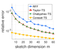
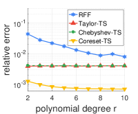
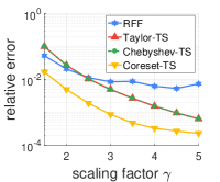
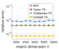
(a) synthetic dataset

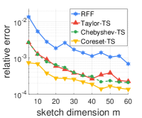
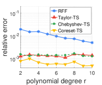
(b)  $\mathtt{segment}$ dataset

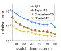
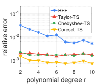
(c)  $\mathtt{usps}$ dataset

Figure 1: Kernel approximation under (a) synthetic, (b)  $\mathtt{segment}$ and (c)  $\mathtt{usps}$ dataset. We set sketch dimension $m=10$, polynomial degree $r=10$ and coreset size $k=10$ unless stated otherwise. All test methods have comparable running times.

Table 1: Classification error, kernel approximation error and speedup for classification (training time) with kernel SVM under various real-world datasets.

Dataset	Statistics		Classification error (%)			Kernel approximation error		Speedup
	$n$	$d$	Exact	RFF	Coreset-TS	RFF	Coreset-TS	Coreset-TS
$\mathtt{segment}$	$2{,}310$	$19$	$3.20$	$3.28$	$3.22$	$1.7\times 10^{-3}$	$3.21\times 10^{-4}$	$8.26$
$\mathtt{satimage}$	$4{,}335$	$36$	$23.54$	$24.11$	$23.74$	$6.5\times 10^{-3}$	$3.54\times 10^{-3}$	$10.06$
$\mathtt{anuran}$	$7{,}195$	$22$	$37.26$	$40.33$	$37.36$	$6.1\times 10^{-3}$	$3.1\times 10^{-4}$	$49.45$
$\mathtt{usps}$	$7{,}291$	$256$	$2.11$	$6.50$	$5.36$	$1.2\times 10^{-3}$	$1.61\times 10^{-4}$	$27.15$
$\mathtt{grid}$	$10{,}000$	$12$	$3.66$	$18.27$	$15.99$	$2.34\times 10^{-3}$	$1.02\times 10^{-3}$	$4.23$
$\mathtt{mapping}$	$10{,}845$	$28$	$15.04$	$18.57$	$17.35$	$6.09\times 10^{-3}$	$2.84\times 10^{-4}$	$4.17$
$\mathtt{letter}$	$20{,}000$	$16$	$2.62$	$11.38$	$10.30$	$3.06\times 10^{3}$	$1.29$	$40.60$

4.1 RBF Kernel Approximation

Given $U=[\boldsymbol{u}_{1},\dots,\boldsymbol{u}_{n}]^{\top}\in\mathbb{R}^{n\times d}$, the RBF kernel $K=[K_{ij}]$ is defined as $K_{ij}:=\exp(-\|\boldsymbol{u}_{i}-\boldsymbol{u}_{j}\|_{2}^{2}/\gamma)$ for $i,j\in[n]$ and $\gamma>0$. It can be represented using the element-wise matrix exponential function:

$$K=Z\exp^{\odot}(2UU^{\top}/\gamma)Z,$$ (4.1)

where $Z$ is the $n$-by-$n$ diagonal matrix with $Z_{ii}=\exp(-\left\lVert\boldsymbol{u}_{i}\right\rVert_{2}^{2}/\gamma)$. One can approximate the element-wise matrix function $\exp^{\odot}(2UU^{\top}/\gamma)\approx\Gamma$ where $\Gamma$ is the output of Poly-TensorSketch with $f(x)=\exp(2x/\gamma)$ and $K\approx Z\Gamma Z$. The RBF kernel has been used in many applications including classification (Pennington et al., 2015), covariance estimation (Wang et al., 2015), Gaussian process (Rasmussen, 2003), determinantal point processes (Affandi et al., 2014) where they commonly require multiplications between the kernel matrix and vectors.

For synthetic kernels, we generate random matrices $U\in\mathbb{R}^{1{,}000\times 50}$ whose entries are drawn from the normal distribution $\mathcal{N}(0,1/{50})$. For real-world kernels, we use  $\mathtt{segment}$ and  $\mathtt{usps}$ datasets. We report the average of relative error for $n^{2}$ entries of $K$ under varying parameters, i.e., sketch dimension $m$ and polynomial degree $r$. We choose $m=10$, $r=10$ and $k=10$ as the default configuration. We compare our algorithm, denoted by Coreset-TS, (i.e., Poly-TensorSketch using the coefficient computed as described in Section 3.3) with the random Fourier feature (RFF) (Rahimi & Recht, 2008) of the same computational complexity, i.e., its embedding dimension is chosen to $mr$ so that the rank of their approximated kernels is the same and their running times are comparable. We also benchmark Poly-TensorSketch using coefficients from Taylor and Chebyshev series expansions which are denoted by Taylor-TS and Chebyshev-TS, respectively. As reported in Figure 1, we observe that Coreset-TS consistently outperforms the competitors under all tested settings and datasets, where its error is often at orders of magnitude smaller than that of RFF. In particular, observe that the error of Coreset-TS tends to decreases with respect to the polynomial degree $r$, which is not the case for Taylor-TS and Chebyshev-TS (suboptimal versions of our algorithm). We additionally perform the Poly-TensorSketch using the optimal coefficient and compare it with Coreset-TS in the supplementary material.

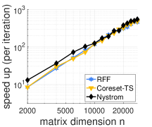
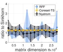
Figure 2: Speedup per iteration (a) and the ratio to Sinkhorn objective (b) of our algorithm, RFF and Nystrom approximation averaged over $3$ tested images in (c). The Sinkhorn algorithm transforms the color information of source images to targets.

4.2 Classification with Kernel SVM

Next, we aim for applying our algorithm (Coreset-TS) to classification tasks using the support vector machine (SVM) based on RBF kernel. Given the input data $U\in\mathbb{R}^{n\times d}$, our algorithm can find a feature $T_{U}\in\mathbb{R}^{n\times m^{\prime}}$ such that $K\approx T_{U}T_{U}^{\top}$ where $K$ is the RBF kernel of $U$ (see Section 4.1). One can expect that a linear SVM using $T_{U}$ shows a similar performance compared to the kernel SVM using $K$. However, for $m^{\prime}\ll n$, the complexity of a linear SVM is much cheaper than that of the kernel method both for training and testing. In order to utilize our algorithm, we construct $T_{U}=\left[\sqrt{c_{0}}T_{U}^{(0)}\dots\sqrt{c_{r}}T_{U}^{(r)}\right]$ where $T_{U}^{(0)},\dots,T_{U}^{(r)}$ are the TensorSketchs of $U$ in Algorithm 2. Here, the coefficient $c_{j}$ should be positive and one can compute the optimal coefficient (3.2) by adding non-negativity condition, which is solvable using simple quadratic programming with marginal additional cost.

We use the open-source SVM package (LIBSVM) (Chang & Lin, 2011) and compare our algorithm with the kernel SVM using the exact RBF and the linear SVM using the embedded feature from RFF of the same running time with ours. We run all experiments with $10$ cross-validations and report the average of the classification error on the validation dataset. We set $m=20$ for the dimension of sketches and $r=3$ for the degree of the polynomial. Table 1 summarizes the results of classification errors, kernel approximation errors and speedups of our algorithm under various real-world datasets. Ours (Coreset-TS) shows better classification errors compared to RFF of comparable running time and runs up to $50$ times faster than the exact method. We also observe that large $m$ can improve the performance (see the supplementary material).

4.3 Sinkhorn Algorithm for Optimal Transport

We apply Coreset-TS to the Sinkhorn algorithm for computing the optimal transport distance (Cuturi, 2013). The algorithm is the entropic regularization for approximating the distance of two discrete probability density. It is a fixed-point algorithm where each iteration requires multiplication of an element-wise matrix exponential function with a vector. More formally, given $\boldsymbol{a},\boldsymbol{b}\in\mathbb{R}^{n}$, and two distinct data points of the same dimension $\{\boldsymbol{x}_{i}\}_{i=1}^{n}$, $\{\boldsymbol{y}_{j}\}_{j=1}^{n}$, the algorithm iteratively computes $\boldsymbol{u}=\boldsymbol{a}\oslash\left(\exp^{\odot}(-\gamma D)\boldsymbol{v}\right)$ and $\boldsymbol{v}=\boldsymbol{b}\oslash\left(\exp^{\odot}(-\gamma D)^{\top}\boldsymbol{u}\right)$ for some initial $\boldsymbol{v}$ where $D_{ij}:=\|\boldsymbol{x}_{i}-\boldsymbol{y}_{j}\|_{2}^{2}$ and $\oslash$ denotes the element-wise division. Hence, the computation can be efficiently approximated using our algorithm or RFF. We also perform the Nyström approximation (Williams & Seeger, 2001) which was recently used for developing a scalable Sinkhorn algorithm (Altschuler et al., 2019). We provide all the details in the supplementary materials.

Given a pair of source and target images as shown in Figure 2 (c), we randomly sample $\{\boldsymbol{x}_{i}\}_{i=1}^{n}$ from RGB pixels in the source image and $\{\boldsymbol{y}_{j}\}_{j=1}^{n}$ from those in the target image. We set $m=20,d=3,r=3$ and $\gamma=1$. Figure 2 (a) reports the speedup per iteration of the tested approximation algorithms over the exact computation and Figure 2 (b) shows the ratios the objective value of the approximated Sinkhorn algorithm to the exact one after $10$ iterations. As reported in Figure 2 (a), all algorithms run at orders of magnitude faster than the exact Sinkhorn algorithm. Furthermore, the approximation ratio of ours is much more stable, while both RFF and Nyström have huge variances without any tendency on the dimension $n$.

Table 2: Test errors on MNIST of linearization of $2$-layer neural network, i.e., $W_{2}\mathtt{sigmoid}^{\odot}(W_{1}\boldsymbol{x})\approx(W_{2}T_{W_{1}})T_{\boldsymbol{x}}$ where the input and hidden dimensions are $d=784$, $d_{h}=800$, respectively, and the degree $r=3$.

Model	Complexity	$m$	Error ($\%$)
$W\boldsymbol{x}$	$\mathcal{O}(d)$	$-$	$9.13$
$(W_{2}T_{W_{1}})T_{\boldsymbol{x}}$	${\mathcal{O}}(r(d+m\log m))$	$100$	$11.45$
		$200$	$9.07$
		$400$	$8.08$
		$800$	$7.62$
$W_{2}\mathtt{sigmoid}^{\odot}(W_{1}\boldsymbol{x})$	$\mathcal{O}(d_{h}d)$	$-$	$2.29$

4.4 Linearization of Neural Networks

Finally, we demonstrate that our method has a potential to obtain a low-complexity model by linearization of a neural network. To this end, we consider $2$ fully-connected layers in AlexNet (Krizhevsky et al., 2012) where each has $1{,}024$ hidden nodes and it is trained on CIFAR100 dataset (Krizhevsky et al., 2009). Formally, given an input $\boldsymbol{x}\in\mathbb{R}^{1{,}024}$, its predictive class corresponds to $\arg\max_{i}\left[W_{2}\ \mathtt{sigmoid}^{\odot}(W_{1}\boldsymbol{x})\right]_{i}$ where $W_{1}\in\mathbb{R}^{1{,}024\times 1{,}024},W_{2}\in\mathbb{R}^{1{,}024\times 100}$ are model parameters. We first train the model for $300$ epochs using ADAM optimizer (Kingma & Ba, 2015) with $0.0005$ learning rate. Then, we approximate $\mathtt{sigmoid}^{\odot}(W_{1}\boldsymbol{x})\approx T_{W_{1}}T_{\boldsymbol{x}}$ for $T_{W_{1}}\in\mathbb{R}^{800\times mr},T_{\boldsymbol{x}}\in\mathbb{R}^{mr}$ using Coreset-TS. After that, we fine-tune the parameters $T_{W_{1}},W_{2}$ for $200$ epochs and evaluate the final test error as reported in Table 2. We choose $r=3$ and explore various $m\in\{100,200,400,800\}$. Observe that the obtained model $(W_{2}T_{W_{1}})T_{\boldsymbol{x}}$ is linear with respect to $T_{\boldsymbol{x}}$ and its complexity (i.e., inference time) is much smaller than that of the original neural network. Moreover, by choosing the sketch dimension $m$ appropriately, its performance is better than that of the vanilla linear model $W\boldsymbol{x}$ as reported in Table 2. The results shed a broad applicability our generic approximation scheme and more exploration on this line would be an interesting direction in the future.

5 Conclusion

In this paper, we design a fast algorithm for sketching element-wise matrix functions. Our method is based on combining (a) a polynomial approximation with (b) the randomized matrix tensor sketch. Our main novelty is on finding the optimal polynomial coefficients for minimizing the overall approximation error bound by balancing the errors of (a) and (b). We expect that the generic scheme would enjoy a broader usage in the future.

Appendix A Greedy $k$-center Algorithm

We recall greedy $k$-center algorithm runs in $\mathcal{O}(ndk)$ time given $\boldsymbol{u}_{1},\dots,\boldsymbol{u}_{n}\in\mathbb{R}^{d}$ since it computes the distances between the inputs and the selected coreset $k$ times. The greedy $k$-center was originally studied for set cover problem with $2$-approximation ratio (Vazirani, 2013). Beyond the set cover problem, it has been reported to be useful in many clustering applications. Due to its simple yet efficient clustering performance, we adopt this to approximate the optimal coefficient (3.2) (see Section 3.3).

Appendix B t-SNE plots of Real-world Datasets

The error analysis in Theorem 7 depends on the upper bound of the distortion of input matrix, i.e., $\varepsilon$ of $\varepsilon$-coreset (see Section 3.3). We recall that a smaller $\varepsilon$ gives tighter the error bound (Theorem 7) and this indeed occurs in read-world settings. To verify this, we empirically investigate the t-SNE plot (Maaten & Hinton, 2008) for real-world datasets including  $\mathtt{segment}$ ,  $\mathtt{satimage}$ and  $\mathtt{usps}$ in Figure 3. Observe that data points in t-SNE are well-clustered and it is expected that the distortion $\varepsilon$ are small. This can justify to utilize our coreset-based coefficient construction (Algorithm 3 and 4) for real-world problems.

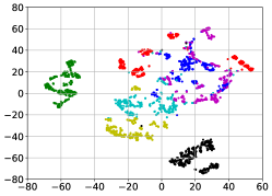
(a)  $\mathtt{segment}$ 

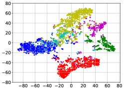
(b)  $\mathtt{satimage}$ 

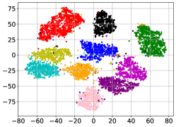
(c)  $\mathtt{usps}$ 

Figure 3: t-SNE plot of (a)  $\mathtt{segment}$ , (b)  $\mathtt{satimage}$ and (c)  $\mathtt{usps}$ datasets. Different colors represent distinguish clusters.

Appendix C Scalable Sinkhorn Algorithm via Nyström Method

Recently, Altschuler et al. (2019) proposed a scalable Sinkhorn algorithm based on Nyström approximation. Motivated by their work, we compare our Coreset-TS to the Nyström method as fast Sinkhorn approximations. In a nutshell, the Nyström method randomly samples a subset $S\subseteq[n]$ such that $|S|=s$ and approximates the kernel matrix $K\in\mathbb{R}^{n\times n}$ as

$$K~{}\approx~{}\widetilde{K}:=K_{[n],S}(K_{S,S})^{\dagger}K_{S,[n]}$$

where $K_{A,B}\in\mathbb{R}^{n\times s}$ is defined as the sub-matrix of $K$ whose rows and columns are indexed by $A,B\subseteq[n]$, respectively, and $K^{\dagger}$ is the pseudo-inverse of a matrix $K$. Observe that given $K_{[n],S}$ and $(K_{S,S})^{\dagger}$ multiplications $\widetilde{K}$ with vectors can be computed efficiently in $\mathcal{O}(ns)$ time for $|S|=s$. It is easy to check that the approximation takes $\mathcal{O}(nds+ns^{2}+s^{3})$ time and remind that ours is $\mathcal{O}(nk(d+r^{2})+r^{3}+nr(d+m\log m))$. Thus, for comparable complexity, we choose $s=\lceil\max(\sqrt{rm},r)\rceil$ for the Nyström method and report the results in Section 4.3.

Appendix D Comparison between Coreset-based Estimation and Optimal Coefficient

The optimal coefficients $\boldsymbol{c}^{*}$ (3.2) can provide a smaller approximation error than that computed using the coreset $\boldsymbol{c}^{\prime}$ (3.3), where a larger $k$ (number of clusters) guarantees a smaller gap, i.e., $\left\lVert\boldsymbol{c}^{*}-\boldsymbol{c}^{\prime}\right\rVert_{2}$. We additionally evaluate the coefficient gap and their kernel approximation errors under the  $\mathtt{segment}$ data, varying $k$ from $5$ to $30$ as reported in Table 3. Observe that a larger $k$ reduces not only the coefficient gap but also kernel error of the coreset. We use $k=10$ for all reported experiments in our paper since the improvement on the kernel error for $k>10$ tends to be marginal.

Table 3: Kernel approximation error between the optimal coefficient and the coreset-based estimation under  $\mathtt{segment}$ data. The optimal coefficient achieves the kernel approximation error of $5.17\times 10^{-4}$ .

$k$	Coefficient gap	Kernel approximation error by coreset
$5$	$3.28\times 10^{-1}$	$5.52\times 10^{-4}$
$10$	$1.72\times 10^{-1}$	$5.39\times 10^{-4}$
$15$	$1.31\times 10^{-1}$	$5.33\times 10^{-4}$
$20$	$1.15\times 10^{-1}$	$5.34\times 10^{-4}$
$25$	$9.07\times 10^{-2}$	$5.28\times 10^{-4}$
$30$	$8.01\times 10^{-2}$	$5.23\times 10^{-4}$

Appendix E Classification with Kernel SVM using Other Parameters

In Section 4.2, we use the sketch dimension $m=20$ but a larger $m$ can reduce the classification error of both Random Fourier Features (RFF) and Coreset-TS, while it increases both time and memory complexity. We additionally conduct experiments with $m=50$ under the last $4$ datasets in Table 1 and report the result in Table 4.

Table 4: Classification error of kernel SVM with $m=20$ and $50$ under $4$ real-world datasets. A larger $m$ shows better classification errors for both RFF and Coreset-TS.

Dataset	Classification error (%)
	RFF		Coreset-TS
	$m=20$	$m=50$	$m=20$	$m=50$
$\mathtt{usps}$	$6.50$	$3.55$	$5.36$	$3.33$
$\mathtt{grid}$	$18.27$	$11.78$	$15.99$	$11.17$
$\mathtt{mapping}$	$18.57$	$17.64$	$17.35$	$17.11$
$\mathtt{letter}$	$11.38$	$5.31$	$10.30$	$5.13$

Appendix F Proofs

F.1 Proof of Proposition 2

Proof. Let $p_{r}(x)=\sum_{j=0}^{r}c_{j}x^{r}$ and $[p_{r}^{\odot}(A)]_{ij}=p_{r}(A_{ij})$. Consider the approximation error into the error from (1) polynomial approximation and (2) tensor sketch:

$$\mathbf{E}\left[\left\lVert f^{\odot}(UV^{\top})-\Gamma\right\rVert_{F}^{2}\right] \leq\mathbf{E}\left[2\left\lVert f^{\odot}(UV^{\top})-p_{r}^{\odot}(UV^{\top})\right\rVert_{F}^{2}+2\left\lVert p_{r}^{\odot}(UV^{\top})-\Gamma\right\rVert_{F}^{2}\right]$$

$$=2\left\lVert f^{\odot}(UV^{\top})-p_{r}^{\odot}(UV^{\top})\right\rVert_{F}^{2}+2\mathbf{E}\left[\left\lVert p_{r}^{\odot}(UV^{\top})-\Gamma\right\rVert_{F}^{2},\right]$$

where the inequality comes from that $(a+b)^{2}\leq 2(a^{2}+b^{2})$ for $a,b\in\mathbb{R}$. The first error is straightforward from the assumption:

$$\left\lVert f^{\odot}(UV^{\top})-\Gamma\right\rVert_{F}^{2} =\sum_{i,j}\left(f\left((UV^{\top})_{ij}\right)-p_{r}\left((UV^{\top})_{ij}\right)\right)^{2}\leq n^{2}\varepsilon^{2}$$

For the second error, we use Theorem 1 to have

$$\mathbf{E}\left[\left\|p_{r}^{\odot}(UV^{\top})-\Gamma\right\|_{F}^{2}\right] \leq r\sum_{j=1}^{r}c_{j}^{2}\ \mathbf{E}\left[\left\|(UV^{\top})^{\odot j}-T_{U}^{(j)}{T_{V}^{(j)}}^{\top}\right\|_{F}^{2}\right]$$

$$\leq r\sum_{j=1}^{r}c_{j}^{2}\frac{(2+3^{j})\left(\sum_{i}(\sum_{k}U_{ik}^{2})^{j}\right)\left(\sum_{i}(\sum_{k}V_{ik}^{2})^{j}\right)}{m}$$

Putting all together, we conclude the result and this completes the proof of Proposition 2.  

F.2 Proof of Lemma 4

Proof. We recall that $\Gamma=\sum_{j=0}^{r}c_{j}T_{U}^{(j)}T_{V}^{(j)\top}.$ and similar to the proof of Proposition 2 we have

$$\mathbf{E}\left[\left\lVert f^{\odot}(UV^{\top})-\Gamma\right\rVert_{F}^{2}\right] \leq 2\left\lVert f^{\odot}(UV^{\top})-p_{r}^{\odot}(UV^{\top})\right\rVert_{F}^{2}+2\mathbf{E}\left[\left\lVert p_{r}^{\odot}(UV^{\top})-\Gamma\right\rVert_{F}^{2},\right]$$

where the inequality comes from that $(a+b)^{2}\leq 2(a^{2}+b^{2})$. The error in the first term can be written as

$$\left\lVert f^{\odot}(UV^{\top})-p_{r}^{\odot}(UV^{\top})\right\rVert_{F}^{2} =\sum_{i,j}\left(f\left((UV^{\top})_{ij}\right)-p_{r}\left((UV^{\top})_{ij}\right)\right)^{2}=\left\|X\mathbf{c}-\mathbf{f}\right\|_{2}^{2}$$

where we recall the Definition 3, that is,

$$X:=\begin{bmatrix}1&[UV^{\top}]_{11}&[UV^{\top}]_{11}^{2}&\dots&[UV^{\top}]_{11}^{r}\\ 1&[UV^{\top}]_{12}&[UV^{\top}]_{12}^{2}&\dots&[UV^{\top}]_{12}^{r}\\ \vdots&\vdots&\vdots&\ddots&\vdots\\ 1&[UV^{\top}]_{nn}&[UV^{\top}]_{nn}^{2}&\dots&[UV^{\top}]_{nn}^{r}\end{bmatrix}\in\mathbb{R}^{n^{2}\times(1+r)}$$

(i.e., also known as the Vandermonde matrix) and $\mathbf{f}\in\mathbb{R}^{n^{2}}$ is the vectorization $f\left((UV^{\top})_{ij}\right)$. For the second error, we use Theorem 1 to have

$$\mathbf{E}\left[\left\|p_{r}^{\odot}(UV^{\top})-\Gamma\right\|_{F}^{2}\right] \leq r\sum_{j=1}^{r}c_{j}^{2}\ \mathbf{E}\left[\left\|(UV^{\top})^{\odot j}-T_{U}^{(j)}{T_{V}^{(j)}}^{\top}\right\|_{F}^{2}\right]$$

$$\leq r\sum_{j=1}^{r}c_{j}^{2}\frac{(2+3^{k})\left(\sum_{i}(\sum_{k}U_{ik}^{2})^{j}\right)\left(\sum_{i}(\sum_{k}V_{ik}^{2})^{j}\right)}{m}=\|W\mathbf{c}\|_{2}^{2}$$

where $W\in\mathbb{R}^{(r+1)\times(r+1)}$ is defined as a diagonal matrix with (see Definition 3)

$$W_{ii}=\begin{dcases}\sqrt{\frac{r(2+3^{k})}{m}\left(\sum_{j}(\sum_{k}U_{jk}^{2})^{i}\right)\left(\sum_{j}(\sum_{k}V_{jk}^{2})^{i}\right)}\quad&i=2,\dots,r+1\\ 0,&i=1.\end{dcases}$$

Putting all together, we have the results, that is,

$$\mathbf{E}\left[\left\lVert f^{\odot}(UV^{\top})-\Gamma\right\rVert_{F}^{2}\right] \leq 2\left(\left\lVert X\boldsymbol{c}-\boldsymbol{f}\right\rVert_{2}^{2}+\left\lVert W\boldsymbol{c}\right\rVert_{2}^{2}\right).$$

This completes the proof of Lemma 4.  

F.3 Proof of Theorem 5

Proof. We denote that

$$g(\boldsymbol{c}):=\|X\boldsymbol{c}-\boldsymbol{f}\|_{2}^{2}+\|W\boldsymbol{c}\|_{2}^{2}=\boldsymbol{c}^{\top}(X^{\top}X+W^{\top}W)\boldsymbol{c}-2\boldsymbol{f}^{\top}X\boldsymbol{c}+\boldsymbol{f}^{\top}\boldsymbol{f}$$

for $\boldsymbol{c}\in\mathbb{R}^{r+1}$ and substituting ${\boldsymbol{c}^{*}}=(X^{\top}X+W^{\top}W)^{-1}X^{\top}\boldsymbol{f}$ into the above, we have

$$g(\boldsymbol{c}^{*}) =\boldsymbol{f}^{\top}\left(I-X(X^{\top}X+W^{\top}W)^{-1}X^{\top}\right)\boldsymbol{f}$$

$$\leq\|I-X(X^{\top}X+W^{\top}W)^{-1}X^{\top}\|_{2}\|\boldsymbol{f}\|_{2}^{2}$$ (F.1)

Since $X^{\top}X$ is positive semi-definite, it has eigendecomposition as $X^{\top}X=V\Sigma V^{\top}$ and $X=\Sigma^{1/2}V^{\top}$. Then, we have

$$X(X^{\top}X+W^{\top}W)^{-1}X^{\top} =\Sigma^{1/2}V^{\top}\left(V\Sigma V^{\top}+W^{\top}W\right)^{-1}V^{\top}\Sigma^{1/2}$$

$$=\left(I+\Sigma^{-1/2}V^{\top}W^{\top}WV\Sigma^{-1/2}\right)^{-1}.$$

For simplicity, let $M:=\Sigma^{-1/2}V^{\top}W^{\top}WV\Sigma^{-1/2}$ and observe that $M$ is symmetric and positive semi-defnite because $W$ is a diagonal and $W_{ii}\geq 0$ for all $i$ (see Definition 3). Then, we have

$$\left\lVert I-(I+M)^{-1}\right\rVert_{2}=\left\lVert M(I+M)^{-1}\right\rVert_{2}=\frac{\left\lVert M\right\rVert_{2}}{1+\left\lVert M\right\rVert_{2}}=\left(1+\left\lVert M\right\rVert_{2}^{-1}\right)^{-1}$$ (F.2)

since $x/(1+x)$ is a increasing function. From the submultiplicativity of $\left\lVert\cdot\right\rVert_{2}$, we have

$$\left\lVert M\right\rVert_{2} =\left\lVert\Sigma^{-1/2}V^{\top}W^{\top}WV\Sigma^{-1/2}\right\rVert_{2}$$

$$\leq\left\lVert\Sigma^{-1/2}\right\rVert_{2}\left\lVert V^{\top}\right\rVert_{2}\left\lVert W^{\top}W\right\rVert_{2}\left\lVert V\right\rVert_{2}\left\lVert\Sigma^{-1/2}\right\rVert_{2}$$

$$=\left\lVert\Sigma^{-1}\right\rVert_{2}\left\lVert W^{\top}W\right\rVert_{2}.$$ (F.3)

where the last equality is from $\left\lVert V\right\rVert_{2}=1$. We remind that

$$W_{ii}=\sqrt{\frac{r(2+3^{i})(\sum_{j}(\sum_{k}U_{jk}^{2})^{i})(\sum_{j}(\sum_{k}V_{jk}^{2})^{i})}{m}}$$

for $i\in 2,\dots,r+1$ and $W_{1,1}=0$. Therefore,

$$\left\lVert W^{\top}W\right\rVert_{2} =\max_{i}W_{ii}^{2}$$

$$=\frac{r}{m}\underbrace{\max\left(5\|U\|_{F}^{2}\|V\|_{F}^{2},(2+3^{r})\left(\sum_{j}\left(\sum_{k}U_{jk}^{2}\right)^{r}\right)\left(\sum_{j}\left(\sum_{k}V_{jk}^{2}\right)^{r}\right)\right)}_{:=C}=\frac{rC}{m}$$

and recall that $\sigma\geq 0$ is denoted by the smallest singular value of $X$. Then, $\|\Sigma^{-1}\|_{2}\leq 1/\sigma^{2}$. Substituting the above bounds on $\left\lVert W^{\top}W\right\rVert_{2},\left\lVert\Sigma^{-1}\right\rVert_{2}$ into (F.3), we have

$$\|M\|_{2}\leq\frac{rC}{m\sigma^{2}}$$

and putting this bound and (F.2) into (F.3), we have that

$$g(\boldsymbol{c}^{*})\leq\left(1+\frac{m\sigma^{2}}{rC}\right)^{-1}\left\lVert\boldsymbol{f}\right\rVert_{2}^{2}=\left(1+\frac{m\sigma^{2}}{rC}\right)^{-1}\left\lVert f^{\odot}(UV^{\top})\right\rVert_{F}^{2}.$$

Combining this with Lemma 4, we obtained the proposed bound. This completes the proof of Theorem 5.  

F.4 Proof of Theorem 7

Recall that $P:[n]\rightarrow[k]$ is a mapping that satisfies with

$$\sum_{i=1}^{n}\left\lVert\boldsymbol{u}_{i}-\boldsymbol{u}_{P(i)}\right\rVert_{2}\leq\varepsilon,$$

for some $\varepsilon>0$ where $\boldsymbol{u}_{i},\boldsymbol{v}_{i}$ are the $i$-th row of $U,V$, respectively. Let $r(x):=f(x)-\sum_{i=0}^{r}c_{i}x^{i}$. Then,

$$\left|{\left\lVert X\boldsymbol{c}-\boldsymbol{f}\right\rVert_{2}^{2}-\left\lVert D^{1/2}(\overline{X}\boldsymbol{c}-{\overline{\boldsymbol{f}}})\right\rVert_{2}^{2}}\right| =\left|{\sum_{i,j=1}^{n}r(\boldsymbol{u}_{i}^{\top}\boldsymbol{v}_{j})^{2}-\sum_{\ell=1}^{k}\sum_{j=1}^{n}|P_{\ell}|\cdot r(\boldsymbol{u}_{\ell}^{\top}\boldsymbol{v}_{j})^{2}}\right|$$ (F.4)

$$=\left|{\sum_{i,j=1}^{n}r(\boldsymbol{u}_{i}^{\top}\boldsymbol{v}_{j})^{2}-r(\boldsymbol{u}_{P(i)}^{\top}\boldsymbol{v}_{j})^{2}}\right|$$ (F.5)

$$\leq\sum_{i,j=1}^{n}\left|{r(\boldsymbol{u}_{i}^{\top}\boldsymbol{v}_{j})^{2}-r(\boldsymbol{u}_{P(i)}^{\top}\boldsymbol{v}_{j})^{2}}\right|$$ (F.6)

$$\leq\sum_{i,j}L\left|{\boldsymbol{u}_{i}^{\top}\boldsymbol{v}_{j}-\boldsymbol{u}_{P(i)}^{\top}\boldsymbol{v}_{j}}\right|$$ (F.7)

$$\leq L\left(\sum_{i=1}^{n}\left\lVert\boldsymbol{u}_{i}-\boldsymbol{u}_{P(i)}\right\rVert_{2}\right)\left(\sum_{j=1}^{n}\left\lVert\boldsymbol{v}_{j}\right\rVert_{2}\right)$$ (F.8)

$$\leq L\varepsilon\left(\sum_{j=1}^{n}\left\lVert\boldsymbol{v}_{j}\right\rVert_{2}\right)$$ (F.9)

From Lemma 4 and Theorem 5, we have that

$$\mathbf{E}\left[\left\lVert f^{\odot}(UV^{\top})-\Gamma\right\rVert_{F}^{2}\right] \leq 2\left(\left\lVert X\boldsymbol{c}-\boldsymbol{f}\right\rVert_{2}^{2}+\left\lVert W\boldsymbol{c}\right\rVert{2}\right)$$

$$\leq 2\left(\left\lVert D^{1/2}(\overline{X}\boldsymbol{c}-{\overline{\boldsymbol{f}}})\right\rVert_{2}^{2}+\left\lVert W\boldsymbol{c}\right\rVert{2}\right)+2L\varepsilon\left(\sum_{j=1}^{n}\left\lVert\boldsymbol{v}_{j}\right\rVert_{2}\right)$$

$$\leq\left(\frac{2}{1+\frac{m\overline{\sigma}}{r\overline{C}}}\right)\left\lVert\overline{\boldsymbol{f}}\right\rVert_{2}^{2}+2L\varepsilon\left(\sum_{j=1}^{n}\left\lVert\boldsymbol{v}_{j}\right\rVert_{2}\right).$$

where $\Gamma$ is the output of Algorithm 2 with the approximated coefficient in (3.3), $\boldsymbol{v}_{i}$ is the $i$-th row of $V$, $\overline{\sigma}$ is the smallest singular value of $D^{1/2}\overline{X}$ and ${C}:=\max(5\|{U}\|_{F}^{2}\|V\|_{F}^{2},(2+3^{r})(\sum_{j}(\sum_{k}{U}_{jk}^{2})^{r})(\sum_{j}(\sum_{k}V_{jk}^{2})^{r}))$. This complete the proof of Theorem 7.