Differentiable Algorithm Networks for
Composable Robot Learning

Abstract

This paper introduces the Differentiable Algorithm Network (DAN), a composable architecture for robot learning systems. A DAN is composed of neural network modules, each encoding a differentiable robot algorithm and an associated model; and it is trained end-to-end from data. DAN combines the strengths of model-driven modular system design and data-driven end-to-end learning. The algorithms and models act as structural assumptions to reduce the data requirements for learning; end-to-end learning allows the modules to adapt to one another and compensate for imperfect models and algorithms, in order to achieve the best overall system performance. We illustrate the DAN methodology through a case study on a simulated robot system, which learns to navigate in complex 3-D environments with only local visual observations and an image of a partially correct 2-D floor map.

I Introduction

There is an essential tension between the model-based and the model-free approaches to robot system design. Robotics research has provided a wealth of powerful models for capabilities including perception, state estimation, planning, and control. Put together, they form the basis of many successful robot systems, from Shakey [36] to Stanley [47]. At the same time, the data-driven, model-free approach, particularly, deep learning, has recently produced exciting results in areas such as vision and object manipulation (see, e.g.,  [6, 30, 34]), tasks in which the model-based approach faces much difficulty despite decades of research. Can we reconcile the seemingly conflicting assumptions of model-based and model-free approaches and integrate the two into a single unified framework?

While the two approaches appear antithetical, they in fact focus on different aspects of robot system design. The model-based approach focuses on the structured, modular representation. We decompose a robotic task into well-understood, interpretable sub-tasks. For each sub-task, we construct a model manually from prior knowledge or learn it from data. We then develop algorithms to infer solutions given the model. Finally, we compose the components into an overall system. The performance of the system may be suboptimal because of imperfect models, approximate algorithms, or a poorly chosen decomposition. In contrast, the model-free approach relies on end-to-end training with powerful function approximators. We approximate the robot policy or controller with a rich parameterized function; we learn all parameters jointly from data, and optimize for the overall objective. A key issue here is to choose the approximating function class. We need the right prior, or bias, to moderate the data requirements for learning. We want to combine the strengths of the model-based and model-free approaches by performing end-to-end learning over a structured, modular system representation. Our objectives are (i) to compensate for imperfections in models, algorithms, and decomposition and (ii) achieve strong performance with limited training data.

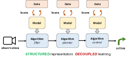
(a)

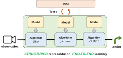
(b)

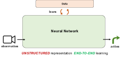
(c)

Figure 1: Three general architectures of robot learning systems. (a) Model-based: structured representation, decoupled learning. (b) DAN: structured representation and end-to-end training. (c) Model-free: unstructured representation, end-to-end learning.

To this end, we introduce the Differentiable Algorithm Network (DAN), a composable architecture for robot learning systems. A DAN is composed of neural network modules encoding differentiable robot algorithms and associated models; and it is trained end-to-end from data. The network architecture is constrained by the algorithms, which act as a structured prior. The network parameters encode the model parameters and tunable algorithm parameters. In contrast with the conventional model-based approach, which learns a model to match the underlying system dynamics, DAN trains the network end-to-end to optimize the overall task objective by allowing network modules, including both models and algorithms, to adapt and compensate for each others’ imperfections. The idea of embedding algorithms in neural networks has appeared many times before (e.g., [4, 3, 15, 18, 19, 20, 25, 26, 27, 28, 29, 39, 40, 43, 37, 38, 45]). Recent studies suggest that even biological nervous systems encode model and algorithm structures, e.g., the Bloom filter [9] in the fruit fly [12]. However, earlier work all focuses on individual algorithm modules rather than composing them for an overall system.

DAN provides a general methodology for composing flexible, robust robot learning systems. We illustrate this methodology through a case study of building a simulated robot system that navigates in complex 3-D environments with only local visual observations and an image of a partially correct 2-D floor map. The architecture of this system includes DAN modules for visual perception, state filtering, planning, and local control. We experiment with several learning strategies and use the results to highlight three main advantages of the DAN methodology.

1. Robustness against imperfect models and algorithms. Strong priors, in this case, model-based algorithms, speed up learning. However, poorly chosen priors may ultimately limit the performance of the learned system. DAN learning systems are robust. Even when the underlying algorithm of a DAN makes simplifying assumptions that are not fully satisfied, such as the Markov property or perfect observations, the overall system can learn a model that compensates for the mismatch between the algorithm’s assumptions and the physical reality.

2. Robustness against imperfect system decomposition. The venerable modularity principle of system design requires us to specify well-defined interfaces to decompose a system into self-contained components. Imperfect independence assumptions may result in suboptimal interface choices. By relaxing the interfaces between modules through learning, DAN improves overall system performance, sometimes significantly.

3. Flexible module representation. Neural networks, treated as computational graphs, provide a rich, flexible representation. While some system modules are naturally represented as an algorithm together with a model, others are more easily represented as a linear feedback controller, finite-state machine, or a recurrent neural network. DAN provides a uniform representation for them all and a standard interface for composing them.

II Related work

The DAN compensates for imperfect model assumptions in a robotic system through end-to-end training. Imperfect models are common in robotic systems. They have been studied widely in various contexts, e.g., to account for uncertainty in the planning model [13, 16, 23, 49, 44] or to directly learn strategies that are robust against imperfections in environment models [11, 2], policies [24, 42], or approximate algorithms [40]. Unlike the earlier work, the DAN commits to the algorithm choices, but adapts the models to compensate for imperfections through end-to-end training from data.

Learning models adapted to a task or an algorithm has been also explored in the past. In the context of MDPs, Farahmand [17] learns transition models adapted to value iteration to compensate for a mis-specified model class. In the context of manipulation, Agrawal et al. [1] learns inaccurate, “intuitive” models that still allow good task performance. In the context of control, Bansal et al. [7] applies Bayesian optimization to learn a transition model directly for the policy. DAN builds on a differentiable representation of algorithms, which scales to learning complex models in large, modular systems jointly.

The idea of encoding algorithms in neural networks has been proposed in various contexts, including state estimation [20, 25, 26, 28], planning [18, 19, 27, 37, 45] and control [4, 15, 38, 39]. DAN generalizes these ideas: it encodes the entire solution structure of a system including multiple model and algorithm components. In this paper we investigate the opportunities the DAN approach opens up in robot system design, where incorrect modelling assumptions are compensated for by using end-to-end learning from data. While prior work shows potential in this direction [27], general DANs with multiple components have not yet been explored.

We study DAN in a visual localization and navigation domain, a challenging robotic task of real importance [14, 5]. While our primary objective is to illustrate the DAN approach, our work can also be seen as a contribution to the state of the art in constructing robust visual navigation systems. Our problem setting features important challenges that are generally not present in related work, e.g., [35, 51]. Specifically, the goal is specified on a map, which requires localizing and planning with respect to the map. The combination of uncertain location, partial map, and visual input makes this a difficult partially observable decision-making problem, which is challenging for both model-based and model-free approaches.

III Differentiable algorithm networks

III-A General Architectures for Robot Learning Systems

There is a broad spectrum of different architectures for robot learning systems, with the purely model-based approach and the purely model-free approach sitting at the extremes (Fig. 1). DAN aims to combine the strengths of both.

The model-based modular system design decomposes a system into well-understood components, such as filters, planners, and controllers, with well-defined interfaces between them (Fig. 1a). There is a clear separation between models and algorithms. Each model is designed or trained independently to match the underlying physical reality. For example, we may learn a probabilistic state-transition model $p(s^{\prime}|s,a)$ for state $s$, action $a$, and next state $s^{\prime}$, given supervised training data $(s_{i},a_{i},s_{i+1}),i=0,1,2,\ldots$ , or learn an observation model $p(o|s)$ for state $s$ and observation $o$, given the data $(s_{i},o_{i}),i=0,1,2,\ldots$ . We learn these models by maximizing the model likelihood of the training data. The model-based approach relies on well-understood, generally correct “independence” assumptions to decompose a system into modules and interfaces. It has produced many successful robot systems.

However, some robot tasks are poorly understood. Identifying the right assumptions for modeling or decomposition is difficult. Consider, for example, folding clothes. We may not know a good representation of latent states. Standard modeling assumptions, such as Markovian state transitions or Gaussian noise, may break down. Large observation spaces, such as camera images, make learning a complete probabilistic distributional model infeasible. In reaction to these difficulties, the model-free, end-to-end approach abandons models completely; instead, it exploits the strong approximation capabilities of a general function approximator, such as a deep neural network, and uses large amounts of data to train end-to-end on the task of interest (Fig. 1c). For example, it may train a neural network policy that directly maps camera images to robot actions for manipulating clothes. The lack of assumptions, however, often comes at the cost of large amounts of training data, reflecting the fundamental trade-off between model assumptions and data.

DAN fuses the model-based and model-free approaches (Fig. 1b). Like the model-based approach, it exploits domain knowledge to design the overall system structure: it embeds model-based algorithms for filtering, planning, and control in a neural network and also maintains the separation between models and algorithms. These structural assumptions provide a strong and useful bias, which reduces the required amount of training data. At the same time, like the model-free approach, DAN trains the entire system end-to-end, thus allowing modules to modify themselves cooperatively to optimize overall task performance and to compensate for any incorrect model assumptions. Further, the uniform neural network representation makes it easy to mix model-based and model-free elements within a single system. For example, we can replace a model-predictive control module with an LSTM [21] or vice versa. inline,color=blue!10]pk: skip last two/one sentences if need space

III-B Differentiable Algorithms

DAN is based on the idea of differentiable algorithms. We view a robot system as a policy $\pi$ that maps observation histories to robot actions. Ultimately we desire a system that performs well according to a suitable metric $\mathcal{J}({\pi})$, e.g., expected total reward. We may obtain $\pi$ by applying an algorithm $\mathcal{A}$ to a model $M$, so that $\pi=\mathcal{A}(M)$. The model $M$ often takes on a parametric form $M(\theta)$ and is learned from data. To construct a DAN, we start with the same conceptual structure, but design a representation of $M(\theta)$ and a neural network function ${F}$, so that ${F}(\theta)\approx\mathcal{A}\bigl{(}M(\theta)\bigr{)}$. Most importantly, $F(\theta)$ is differentiable with respect to $\theta$.

What is the benefit of a differentiable representation of $F(\theta)$? The conventional model learning objective is a form of predictive likelihood $\ell\bigl{(}M(\theta)\bigr{)}$, which is independent of the algorithm $\mathcal{A}$. It is only indirectly connected to the end objective $\mathcal{J}(\pi)$ through $\pi=\mathcal{A}\bigl{(}M(\theta)\bigr{)}$. In contrast, DAN learns by directly optimizing $\mathcal{J}(\pi)=\mathcal{J}\bigl{(}F(\theta)\bigr{)}$. This end-to-end optimization is generally difficult, because it involves $\mathcal{A}$. The differentiable representation of $F(\theta)$ allows for efficient first-order methods, e.g., gradient descent, which back-propagate gradients through the steps of $\mathcal{A}$ encoded in $F(\theta)$.

The premise of the DAN methodology is that many key robot algorithms admit differentiable representations. Prior work has addressed this important question for filtering, planning, and control (see Section II).

A differentiable representation is straightforward if the algorithm contains only differentiable operations. For example, the histogram filter only uses matrix multiplications and summations, which are clearly differentiable. Other algorithms involve non-differentiable operations, such as discrete maximization, sampling, and indexing. One strategy is to replace non-differentiable operations by a differentiable approximation, e.g., replace max by soft-max, sampling by soft-sampling [28], indexing by soft-indexing [27]. A drawback of these new operations is a possible reduction of algorithmic efficiency. Another strategy is to keep non-differentiable nodes in the computation graph, and approximate the gradients, e.g. through sampling methods. An example is the implementation of Monte-Carlo tree search in [19]. Schulman et al. [41] provides a generic framework for optimizing computation graphs with non-differentiable nodes, although gradient estimates can have high variance. Generic variance-reduction techniques are actively being investigated [50]. inline,color=blue!10]pk: remove prev sentence for space Finally, a fundamentally different strategy is to derive analytic gradients around a fixed point output of the algorithm. The idea has been explored in the context of control algorithms [4] and for generic optimization [3, 10]. inline,color=blue!10]pk: shorten for space When applicable, the analytic approach is appealing for its computational efficiency.

III-C Compensating for Approximations: Illustrative Examples

We begin with two simple examples that illustrate DAN’s ability to compensate for imperfect models and algorithms.

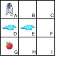
(a)

(b)

Figure 2: Simple illustrative problems.

Puddle-MDP  Consider a tiny grid navigation problem, Puddle-MDP, in Fig. 2a. Actions are to move right, left, up, or down. Reaching the apple ($G$) or a puddle ($D$ and $E$) yields positive and negative rewards, respectively. Starting in state $A$, the best strategy is to move along path $ABCFIHG$, reaching the apple while avoiding puddles. In a model-based approach we may learn transition and reward models, and plan with the value iteration algorithm. If the planning horizon is 6 or greater, we get the optimal policy. However, what if the planning horizon is 4? Value iteration with the perfectly accurate transition and reward models cannot find a way around the puddles. We train a DAN, encoding the horizon-4 value iteration algorithm, and get a surprising result: the learned transition model encodes actions as if they were “macro-actions,” predicting that moving right from state $A$ will land in state $C$, etc.. inline,color=blue!10]pk: evidence While this model is predictively incorrect, it allows value iteration to find the optimal path around the puddles even with a horizon of 4. Similar algorithm approximations are common. As illustrated by this example, DAN may compensate for an approximate algorithm by training models end-to-end.

Puddle-POMDP  We also consider a related problem, shown in Fig. 2b. The robot starts in state $A$, but it does not observe the state afterwards; and actions may fail ($p_{\textrm{fail}}=0.4$), in which case the robot remains in place. The optimal solution is non-trivial. If the robot moves right and down, it will often end up in the puddle due to the transition noise. The optimal policy is to take the right action multiple times, until the state uncertainty is sufficiently reduced, and only then move down. Again, when we learn the “correct” transition and observation models, and use a POMDP-solution method, the optimal strategy is found. POMDP solvers are computationally expensive. Robot systems often decouple state-estimation, and plan with the most likely state. In this problem, having the “correct” models, the decoupled strategy performs poorly: after moving one step to the right, the most likely state is $B$, in which the robot should move down—but there is a substantial chance the robot will have stayed in $A$ and moved into the puddle. We encode the same system, state estimator and planner, in a DAN, and train the models end-to-end, to generate good behaviour instead of accurate predictions. The optimal behavior is recovered. How? The “failure” probability is increased over $0.5$, inline,color=blue!10]pk: evidence so that after moving to the right, the most likely state is still $A$, which causes additional rightward motions before moving down. Similar situations occur in practice: for example, Monte-Carlo localization is known to work better when the transition noise is overestimated [46, p. 118], [26]. Through end-to-end training, DAN may learn similar strategies for compensating modelling approximations. inline,color=blue!10]pk: cut down for space

IV Case study: Learning visual navigation under uncertainty

We investigate the DAN approach in a simulated visual navigation domain. The domain highlights important challenges of robot decision making: acting under state uncertainty, environment uncertainty, and processing rich sensory input. Because of the combination of these challenges, an adequate model-based system design is not immediately available—modelling approximations are necessary. Our case study reveals various ways DAN training may compensate for modelling approximations, even in a moderately large modular system, enabling substantially improved performance.

IV-A Domain Description

A robot is tasked to navigate to a goal in a previously unseen, visually rich 3D environment, using a 2D floor map, and images from an onboard camera. Each environment has different layout and visual appearance. Examples are shown in Fig. 3. The domain involves challenging partial observability: the location of the robot is unknown, and the environment is uncertain, i.e., the map indicates walls, but not other objects, like furniture. Since the goal is specified on the map, the robot must localize, which involves matching features from rich camera images and the 2D map. It must then find a path to the goal, potentially far from its current location, and navigate while detecting and avoiding unknown objects in the environment. We have access to a set of training environments for learning. After learning, the system is evaluated in new, previously unseen environments.

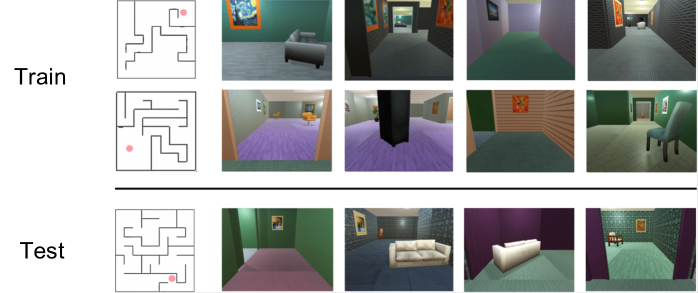
Figure 3: 3D simulation environments for navigation. The location of the robot is not observed. Maps do not indicate objects to be avoided.

We develop a custom-built simulator with the Unity 3D Engine [48] for controlled experiments. The simulator captures the critical challenges in terms of uncertainties and rich visual appearance; however, it does not aim to simulate all aspects of the real-world, such as dynamics. The simulator generates randomized 3-D environments. First, a random $19\times 19$ grid maze is generated that defines the placement of walls in the 3-D environment. Second, additional objects are placed at random locations, but without fully blocking passages. Objects are chosen from a set of 23 common household furniture: chairs, tables, beds, etc. The visual appearance is randomized, including pictures on the walls, textures, colors and lighting. The motion of the robot is simplified: robot states are discrete 2-D coordinates with orientation, and transitions are deterministic. There are a total of 1444 states corresponding to the $19\times 19$ grid and 4 orientations. The robot does not observe the state. It is given a set of possible initial states: in some episodes this includes all states, in some episodes a random subset of all states. Collisions with objects are evaluated based on the robot bounding box of size $0.8\times 0.8$ grid cells. In the event of a collision the state remains unchanged. The actions are: move forward, turn left, turn right, stay. Rewards are $+20$ for reaching the goal; $-10$ for a collision; $-0.1$ for every other action. The discount factor is $0.99$.

We consider variants of the domain with increasing difficulty, as shown in Table I. In Task A, the robot location is directly observed, and the map given to the robot fully describes the environment, including walls and furniture. In Task B, the location is not observed. Instead, the robot receives local (but noise-free) observations indicating the presence of walls or objects in the 3 grid squares in front of the robot. In Task C, the noise-free binary observation vectors are replaced with images from an onboard camera. Finally, Task D is the full domain that involves vision, uncertain location and uncertain environment. The map given to the robot only partially describes the environment: it indicates walls but not the furniture.

IV-B Architecture Description

We experiment with different architectures for systems that learn in this domain. The systems are built by composing up to four generic modules: vision, filtering, planning, and local control (Fig. 4). We explore different implementations and training strategies for each module and combinations of modules. The different versions of the modules appear as entries in our results table (Table II). Details are in the appendix.

	Task A	Task B	Task C	Task D
Map input	full	full	full	without furniture
Observation input	location	vector	image	image
Uncertain robot location		x	x	x
Visual input			x	x
Partially correct map				x

TABLE I: Task variants and challenges involved

Vision  The vision module takes high-dimensional, $80\times 40\times 3$ images as inputs, and outputs a low-dimensional vector representation. We consider two implementations (denoted CNN and CNN-f) to explore the effect of relaxing the interfaces between modules. CNN is a convolutional network [32] with a length-3 binary vector output that indicates the presence of walls and objects in the 3 grid squares in front of the robot; this output is compatible with the observations provided as input in Task B. CNN-f is a similar network that outputs length-16 embedding with no pre-specified semantics.

In Task D, where the map is partial, we use two vision modules: one for estimating location in the map (filtering) and one for local control. The output observation vector in the first case is trained to only indicate walls. In the second case it is expected to indicate all obstacles, both walls and objects. The neural network weights in the two modules are shared except for the last fully-connected layer.

Filtering  The filtering module is a histogram (Bayes) filter [46, 25] that maintains a belief, a probability distribution over the states of the robot, which will be the input to the planner. The default implementation (HF-bel) takes a length-3 observation vector, the action, and previous belief as inputs, and outputs an updated belief (probabilities over states). We also experiment with a version of the filter module (HF-ml) that outputs a one-hot encoding of the most-likely state. In the DAN setting, we use the notation HF to indicate that the semantics of filter output is not enforced. A version that has the richer length-16 feature vectors as input is denoted as f-HF.

The histogram filter uses two parameterized models: an observation model, $Z(o_{t}|s_{t})$, that defines the probability of observations given the state; and a transition model $T(s_{t+1}|s_{t},a_{t})$ that defines the probability of next states given the current state and an action. We represent these models by small neural networks conditioned on the map. Specifically, the observation model combines features from the $19\times 19$ map and the observation vector, and outputs a $1444$-dimensional vector, estimates of the observation likelihood for each state.

The transition model defines $3\times 3\times 4$ local transition probabilities for each state and action pair. We consider two implementations: a heterogeneous model, where local transition probabilities are estimated from the map using a convolution layer; and a homogeneous model that is independent of the map and the states. The parameters in the latter case are the local transition probabilities for each action; this is used in the DAN setting. In the independently learned settings, the transitions are heterogeneous, giving more accurate models.

Planning  We use two planning algorithms: value iteration (VI), a simple method for solving MDPs [8, 45], and SARSOP, a state-of-the-art POMDP planner [31]. Both planners take in a belief vector and output an action. The planners require transition and reward models. Transition models are identical to the histogram filter, alternatively homogeneous or heterogeneous. The reward model, $R(s,a)$, defines rewards for each state action pair. We assume rewards are unknown. The reward model is learned using a two-layer CNN that takes in the map and outputs a $1444$-dimensional reward vector for each action.

VI planning is done by applying Bellman updates for $H$ (horizon) iterations, which provide approximate Q values for each state-action pair. The length-4 action-value outputs are obtained by weighting the Q values for each action with the belief vector. When the belief vector is a one-hot encoded state, this corresponds to taking the Q values for the current state. When the belief vector is a distribution, this strategy is known as the QMDP approximation [33, 27].

We explore a number of variations on VI: long and short horizon, and heterogeneous and homogeneous transition models. We denote them VI-short, VI-hom, and VI-short-hom.

Local control  The local control module takes in an observation vector from the vision module, an action-value vector from the planner, and outputs a new action. We experiment with a hand-built state machine policy (SM) and learned policies, based either on the 3-vector vision output (LSTM) or the richer feature output (f-LSTM).

An alternative to a local control policy is to update the map based on the observations and replan. We denote that case as VI-repl for the planning module, although it can also be thought of as a local-control strategy.

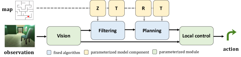
Figure 4: System architecture for visual navigation.

IV-C Training Regimes

We consider two main approaches for training modules: independent, conventional model learning that optimizes for model accuracy; and joint learning that optimizes for the final policy objective end-to-end, using DAN. Both approaches use trajectories from $10,000$ random environments for training, 5 trajectories from each environment.

For independent model learning we use appropriately labelled data tuples: $(o_{t},v_{t})_{i}$ for a vision module, where $o_{t}$ is an image and $v_{t}$ is a local observation vector; $(s_{t},v_{t},M)_{i}$ tuples for an observation model where $M$ is a map; $(s_{t},a_{t},s_{t+1},M)_{i}$ tuples for a transition model; and $(s_{t},a_{t},r_{t},M)_{i}$ tuples for a reward model. The training loss is defined by the appropriate negative log-likelihood of the output.

For end-to-end learning we use expert demonstrations in the form of observation-action trajectories and a map, $(o_{0},a_{0},o_{1},a_{1},...,o_{t},a_{t},M)_{i}$. Expert trajectories are obtained by near-optimal, clairvoyant SARSOP policies that have full knowledge of the underlying environment model. The expert has access to more information than the robot: it uses ground-truth vector observations in Task C and D, and it uses the underlying location of the robot to build a map in Task D. The training loss is the imitation learning objective, i.e., the negative log-likelihood of the expert action for each step along the trajectories. To account for critical but rare events in Task D, we inflated the loss by a factor of 10 when the expert policy had to avoid an unexpected obstacle. We train DANs in a curriculum of increasingly difficult task variants; and pre-train the vision module independently. Details are in Appendix A.

V Experimental results

Quantitative results on different combinations of modules, training strategies and tasks are shown in Table II. Each row corresponds to one experiment. The first two columns characterize the task. The third column describes the architecture and training regime: it lists some subset of the modules V (vision), F (filter), P (planning), and C (local control); the notation DAN(X) means that the modules inside the parentheses are jointly trained to optimize task performance; modules not inside a DAN grouping are either fixed, or have models trained to optimize a predictive objective. The next columns indicate the particular implementation of the component (a detailed list is in Appendix B). Finally, we report the performance of the trained system: the percentage of trials the goal is reached (within 238 steps), the average number of time steps to the goal (only including the successful trials), the percentage of trials that involved one or more collisions, and the total discounted reward averaged over trials. Evaluation is in $500$ randomly generated environments that were not seen during training.

A video is available at https://youtu.be/4jcYlTSJF4Y.

In the following we walk through the experiments, pointing out the most salient results and illustrating a number of ways in which the DAN approach facilitates robot system design. A summary of our findings is in Section V-F.

V-A Task A: Discrete MDP

We begin with a value-iteration algorithm and model representation that are complete for this task (VI*). Whether we train the models independently (A1) or via DAN (A2), the system performs nearly optimally.

We then consider reducing the horizon of value iteration to 25. In this scenario, using independently trained models (A3) performs poorly, because most problem instances require more than 25 steps. Using DAN training (A4), we recover near-optimal performance. As in the Puddle-MDP, DAN learns models that compensate for the weakness of the algorithm: we find that the learned transition model predicts that actions move farther than they actually do.

Learning a transition model that can be different for each state in the domain is costly in space, computation time, and training examples. In many domains, a spatially homogeneous model, which predicts transitions relative to the robot’s current location, will suffice; such models have a relatively small number of parameters and are insensitive to the size of the domain. In our domain, the dynamics are similar in all parts of the space, but do in fact differ locally because of the presence of walls. Experiment A5 illustrates that learning the maximum-likelihood homogeneous transition model and planning with it as if it were exactly correct yields very poor performance. However, applying DAN training to this model (A6) recovers near-optimal performance. Examining the learned models, we see that the penalty for collisions is inflated, causing the robot to select actions that will keep it farther away from obstacles. inline,color=blue!10]pk: evidence

In experiments A7 and A8 we both plan with a shortened horizon and learn a homogeneous transition model, with the now expected poor performance of independently trained models and significant improvement by DAN. We find that, among other things, DAN discovers that it is rarely necessary to take two turn actions in a row; instead, the learned transition model combines the effects of a turn and subsequent move, thus shortening the necessary planning horizon. inline,color=blue!10]pk: evidence

	Map	Observation	Architecture	Vision	Filter	Planner	Control	Success	Time	Collision	Reward
				V	F	P	C	rate	steps	rate
A1	full	state	P			VI*		100%	32.80	0%	12.693
A2	full	state	DAN(P)			VI*		100%	32.80	0%	12.692
A3	full	state	P			VI-short		59.0%	19.50	0%	5.459
A4	full	state	DAN(P)			VI-short		97.8%	34.13	0%	12.049
A5	full	state	P			VI-hom		34.2%	13.88	65.8%	-554.3
A6	full	state	DAN(P)			VI-hom		100%	32.83	0%	12.686
A7	full	state	P			VI-short-hom		33.2%	13.59	60.4%	-510.8
A8	full	state	DAN(P)			VI-short-hom		95.0%	35.82	0%	11.241
B1	full	vector	P			SARSOP		100%	36.12	0%	11.97
B2	full	vector	F + P		HF-ml	VI		94.4%	36.13	11.4%	2.83
B3	full	vector	F + P		HF-bel	VI		63.8%	36.81	0%	4.27
B4	full	vector	DAN(F + P)		HF	VI		99.6%	36.49	0%	11.85
C1	full	image	V+P	CNN		SARSOP		98.4%	38.07	0.6%	11.21
C2	full	image	V+F+P	CNN	HF-ml	VI		95.2%	37.63	13.2%	3.10
C3	full	image	V+F+P	CNN	HF-bel	VI		61.8%	36.18	0.4%	3.89
C4	full	image	V+DAN(F+P)	CNN	HF	VI		97.4%	40.04	0.0%	10.80
C5	full	image	DAN(V+F+P)	CNN	HF	VI		98.8%	36.30	0.8%	11.03
C6	full	image	DAN(V+F+P)	CNN-f	f-HF	VI		99.0%	34.35	0.4%	12.09
D1	partial	image	V+F+P	CNN	HF-ml	VI-repl		89.6%	39.81	7.0%	-29.40
D2	partial	image	V+F+P	CNN	HF-bel	VI-repl		58.4%	36.47	5.4%	-15.64
D3	partial	image	V+F+P+C	CNN	HF-ml	VI	SM	41.4%	29.96	1.8%	-11.18
D4	partial	image	V+F+P+C	CNN	HF-bel	VI	SM	40.0%	29.72	0.8%	-5.42
D5	partial	image	V+F+P+C	CNN	HF-bel	VI	LSTM	66.0%	43.18	4.4%	-15.87
D6	partial	image	V+F+P+C*	CNN	HF-bel	VI	LSTM	76.6%	40.53	3.0%	-12.14
D7	partial	image	V+DAN(F+P)+C	CNN	HF	VI	LSTM	96.4%	45.17	3.6%	8.11
D8	partial	image	V+DAN(F+P)+C*	CNN	HF	VI	LSTM	70.2%	42.34	3.2%	3.60
D9	partial	image	V+DAN(F+P+C)	CNN	HF	VI	LSTM	98.6%	40.55	4.0%	4.12
D10	partial	image	DAN(V+F+P+C)	CNN	HF	VI	LSTM	99.4%	39.60	0.2%	11.09
D11	partial	image	DAN(V+F+P+C)	CNN-f	f-HF	VI	f-LSTM	99.8%	38.05	0.8%	11.43

TABLE II: Main results

V-B Task B: Discrete POMDP

In this setting the robot’s location is not observed. Instead it receives local (but noise-less) length-3 observation vectors. The task can be perfectly modelled by a parameterized POMDP, conditioned on the map. We begin by using a model-class that can represent the domain exactly, learn models independently, and apply SARSOP [31], a near-optimal POMDP solver to the learned models, which yields near-optimal behavior (B1). However, solving a POMDP is expensive (in our case sometimes over $5$ minutes) and it tends to grow doubly exponentially with the horizon. We explore lower-cost, decomposed solutions.

We consider a modular system that decomposes partially observable planning into state estimation with a histogram filter, HF, plus fully observable planning with value iteration, VI. The HF depends on observation and transition models, and VI on transition and reward models. We consider two different fixed interfaces between the modules. In B2, we extract the most likely state and perform VI as if the robot were certain it was in that state. The robot tends to reach the goal, but at a cost of frequent collisions. In B3, we initialize the state-occupancy distribution for VI to be the current belief: this corresponds to the QMDP approximation [33], which accounts for current uncertainty, but ignores future uncertainty. We first train the models independently (B3) and find that the system performs poorly. It often gets stuck, oscillating or taking a stay action, because the approximation assumes that state uncertainty will be dispelled after any action, which is not true in this domain.

Using DAN training to jointly optimize models both in the filter and the planner, directly for task performance, can compensate for the strong approximation in the decoupled system, resulting in near-optimal behavior (B4). Because the filter and planner modules are trained jointly, the system is free to adapt the models in a way to optimize the combined system. We observe that the learned reward model has a large cost for the stay action, and the learned transition model differs from the true model in ways that break symmetry, hence gathering information and preventing oscillatory behavior. inline,color=blue!10]pk: evidence

V-C Task C: POMDP with Image Input

In this setting, instead of three-bit noise-free observations, the robot receives images. A full POMDP model that operates in the space of images is intractable. Hence, we add a vision module, in the form of a CNN. In most experiments in this section, its output is a vector of 3 binary classifications with the same expected semantics as inputs in Task B.

We begin with a classic architecture, in which the vision module is trained via supervised learning, and the observation, transition, and reward models from B1 are used to generate a near-optimal POMDP policy, mapping sequences of outputs from the vision module into actions. C1 shows that reasonable performance can be obtained this way, although a large amount of computation is needed to solve for the policy, and there are failures due to imperfect vision.

We attempt to reduce computational complexity by combining the independently trained vision module with both a most-likely-state, and a QMDP approximation, based on independently trained models (C2 and C3). We obtain performance similar to B2 and B3. Applying DAN training to just the F and P modules (C4) improves performance. Applying DAN to the whole composition of V, F, and P (C5) further improves performance. In each case, we have relaxed the semantics of the interfaces between modules. In C5, we believe the DAN learns to capture the prediction confidence of vision in the observation model allowing increased robustness.

Finally, we relax the constraint on the interface between vision and state estimation. Instead of going through a binary classification vector, we allow the DAN to learn an observation model for state estimation directly using features extracted from images. Performance further improves, even beyond C1. In particular, the goal is reached in fewer steps. This implies that, by removing the interface constraint, the DAN learns to extract more information from images for faster localization—the images, in fact, contain more information than just the occupancy of the three cells in front of the robot.

V-D Task D: POMDP with Image and Partial Map Input

In this setting the maps given to the robot no longer perfectly describe the environment: they indicate walls, but not the furniture. Even without the problems of image processing, the partially observable decision-making problem is intractable: both the robot state and the environment are partially observed, resulting in an $N\times 2^{N}$-dimensional belief space for $N$ grid cells. It is also not clear how the problem can be decomposed.

One simple strategy is to try the same architectures as for Task C. Unmodified, they fail disastrously, as the robot repeatedly attempts to move through unmodeled obstacles. A simple idea is to put newly encountered obstacles into the map—but this solution presupposes that the robot is localized! D1 and D2 show the results of updating the map as if the robot were at the most likely location and replanning whenever an obstacle is encountered. There is some success with this approach, but with many collisions.

A better strategy is to add a local controller to avoid obstacles, which would select alternative actions if the nominally commanded action would result in collision. We begin by using a simple hand-coded strategy in D3 and D4: it largely avoids collisions, but at the cost of often not reaching the goal. Next, we replace the fixed local controller with an LSTM network that maps the commanded action and the current inputs to an updated action. In D5, we train the LSTM in isolation, with the same distribution of objects, but in a fully observed setting (C). In D6, we train the LSTM in a partially observable setting, with the HF and VI modules from system D3, still in isolation (C*). The learning objective is the same as for training DAN, but only the LSTM is trained. Performance remains poor.

In experiments D7 through D11, we apply the DAN methodology to different groups of subsystems of the full architecture. We find that allowing the system to adapt all of the models and to choose interfaces between the modules gives the best performance. The overall reward very closely rivals the optimal solution in a completely observable version of the problem, even when challenged by image interpretation and incorrect maps.

V-E Unstructured Learning Systems

We have reported on extensive experiments that illustrate how the DAN learning can improve significantly over classical model-learning. In addition, we experimented with standard neural-networks on the same tasks, with the same end-to-end objective and training data as for the DAN systems. We used simple combinations of CNN and LSTM components, and performed a basic search over hyper-parameters. Details are in Appendix C. We report the best achieved results for each task in Table III, which are generally quite poor.

These results are consistent with those from prior work on learning map-based navigation, but in much simpler settings, e.g., [45, 27]. It is, of course, entirely possible that a greater investment in the search over neural network architectures and hyper-parameters, as well as the acquisition of more training data, would result in significantly better performance.

The important message of the DAN approach is that it allows robotics experts to use their prior understanding of the problem, in the form of model-based algorithms, to effectively structure a learning system that has the appropriate bias. Learning is more efficient, both in terms of the engineer’s time to set up the problem, and in terms of robot time to gather data. At the same time flexibility and performance can significantly increase over the traditional model-based learning approach.

[1.0] Map Observation Success Time Collision Reward rate steps rate A full state 92.6% 39.79 9.2% -20.65 B full vector 22.2% 50.40 1.6% -4.86 C full image 38.2% 74.50 82.8% -103.59 D partial image 38.4% 75.97 11.4% -8.94

TABLE III: Results for unstructured neural-network learning

V-F Summary

The experimental results point to several strengths of DAN.

Compensate for approximate algorithms.  In Task A, the state-transition model learns “macro actions” to compensate for an approximate planner with short horizon (A3-A4, A7-A8).

Compensate for model mis-specification.  In Task A, the reward model learns inflated collision penalty to compensate for a transition model assumed to be homogeneous incorrectly (A5-A6, A7-A8).

Compensate for approximate decomposition.  In Task B, the reward model learns to penalize the stay action to compensate for the approximate decomposition of partially observable planning into state estimation and fully observable planning system (B3-B4). Further, in Task C and Task D, the vision model possibly learns to encode uncertainty in its output, and the observation model of the filter learns to take the uncertainty into account. This improves the overall performance of state estimation (C5-C6, D10-D11).

Unify model-based and model-free representations.  In Task D, the model-free LSTM controller module, integrated into and trained jointly with a model-based modular system, learns to select actions that compensate for the incompleteness of the map based on perceptual input (D5-D10).

Together the experimental results suggest that through end-to-end learning, DAN compensates for imperfections in models, algorithms, and system decomposition. Further, DAN substantially outperforms unstructured neural networks on the evaluation tasks, demonstrating the benefits of structured priors through models, algorithms, and system decomposition.

VI Conclusion

DAN represents a first step towards a general methodology for designing and implementing robot learning systems. It combines well-understood structures—models, algorithms, interfaces—with end-to-end learning. This enables DAN to achieve strong performance in the presence of modeling errors, while using only limited training data. Our case study suggests that DAN scales up to moderately complex robotic systems involving multiple common components.

DAN adapts the models to compensate for various imperfections in manually specified structures. The improved task performance comes at the cost of reduced model reusability. This is, however, acceptable, when no alternative better structures are known.

Scalability is a major challenge in applying the DAN methodology in practice. A complex systems results in a large network. Further, the optimization landscape of DANs may be more challenging than that of over-parameterized, unstructured neural networks. To alleviate the difficulty of training, one may add “skip” connections or improve credit assignment [50]. Another interesting direction is to combine classical local model learning with end-to-end learning, possibly in a training curriculum. Related ideas in reinforcement learning are promising [22].

Appendix A Implementation details

We implement DAN modules in Tensorflow. The DAN implementation of HF and VI are based on [27] and [45] with the following differences. In VI we use soft-max for performing Bellman updates; the computed Q values are directly used without an additional fully-connected layer; and our transition, reward and observation models have a different form depending on the task variant and experiment setting, as discussed in the paper.

We train DAN systems end-to-end using expert demonstration data. We use backpropagation through time (BPTT) with gradient clipping. In the partially observable domains the latent belief in DAN is initialized with the true underlying initial belief; however, we do not have access to ground-truth beliefs after the first step.

For more complex tasks we found it necessary to train DANs in multiple stages of curriculum. In each stage DAN is trained end-to-end with expert demonstrations, in increasingly difficult task settings. Specifically, in Task B, we start with a training stage where initial beliefs are set to be certain at the true underlying state (while the true state is still not observed after the first step). The second training stage corresponds to the full Task B setting, i.e., initial beliefs are uniformly distributed across a random subset of the state space. In Task C we use three training stages. We first replace image inputs with binary observations and follow the two training stages of Task B. We then add the vision module to DAN and train further with image observations. In Task D we follow the same training stages as in Task C (but now map inputs are only partially correct).

The vision models in Task C and Task D are pre-trained independently with ground-truth binary observation vectors. CNN-f is obtained by replacing the last, fully-connected layer of a pre-trained CNN model and initializing the new weights randomly. We use L2 regularization for the convolutional layers of CNN and CNN-f.

In each training stage we follow an early stopping with patience strategy. Specifically, we decay the learning rate by factors of 0.8 in multiple steps. The first decay step is executed when the validation loss is not decreasing for 15 consecutive epochs. Four more decay steps are executed when the validation loss is not decreasing for 5 consecutive epochs. Training terminates when the next decay step would be triggered. The model with lowest validation loss is chosen for evaluation.

We use the RMSProp optimizer with 0.9 decay rate. The batch size is set to 100. The initial learning rate is set to 0.001. In Task B and Task C we truncate BPTT at 4 time steps. In Task D the initial learning rate is 0.0005 and we truncate BPPT at 8 time steps. Longer sequences did not improve performance.

We use NVidia GTX1080Ti GPUs. Training required approximately 1–8 GB GPU memory and 6–48 hours depending on the task and training setting.

Appendix B Detailed Module Descriptions

Vision

1. CNN. A convolutional neural network with a length-3 binary vector output that indicates the presence of walls and objects in the 3 grid squares in front of the robot. This output is compatible with the observations provided as input in Task B. The CNN has 3 convolutional layers (3-3-1 kernels and 128-128-1 filters) connected to a fully connected layer that maps to the output vector.

2. CNN-f. A similar network as CNN, but with 16-dimensional feature vector outputs that have no pre-determined semantics.

Filtering

1. HF-bel. Histogram filter that takes in 3-dimensional observation vectors, the last action of the robot, and the previous belief distribution represented by a 1444-dimensional vector. The output is the updated belief distribution. At the beginning of a trajectory the belief is initialized to the true initial belief. The transition model in the DAN implementation is homogeneous, in the independently learned implementation it is heterogeneous.

2. HF-ml. The same histogram filter as above, but with the output transformed into a one-hot vector representing the most likely state.

3. HF. The same histogram filter as HF-bel but when used as a DAN, the output is only constrained to be a distribution, i.e., the vector is normalized, but it is not directly enforced to represent the true belief.

4. f-HF. The same filter as HF with a different observation model that takes in 16 dimensional observation features with undetermined semantics.

Planning

1. VI. The default setting of value iteration. When implemented as a DAN we use the homogeneous transition model, and H=76. When learned independently, we use the heterogeneous transition model and plan until convergence.

2. VI*. Value iteration with a sufficiently long planning horizon (H=200) to guarantee finding the optimal path and an environment-dependent, heterogeneous transition model. The same setting is used in the independent implementation and in DAN.

3. VI-short. Value iteration with a short planning horizon (H=25).

4. VI-hom. Value iteration with a homogeneous transition model and long planning horizon.

5. VI-short-hom. Value iteration with short planning horizon and homogeneous transition model.

6. VI-repl. In this implementation when an obstacle is detected by the vision module it is added to the map according to the current most likely state. Whenever the map is updated we replan, i.e., the $Q$ values are recomputed.

7. SARSOP. The SARSOP planner embodies its own Bayes filter. It directly takes in a length-3 binary observation vector and outputs an action. It uses the same transition and reward models as VI, and the same observation model as HF.

Local control

1. SM. Simple, hand-coded state machine for obstacle avoidance. When the action with the highest value would lead to a collision, it picks one of the turn actions with the higher value. Further, to prevent oscillation, consecutive left-right turns are replaced by a forward action if it does not lead to collision.

2. LSTM. A parameterized module using LSTM. We concatenate the observation vector, the action-value vector and the last action vector, and input them to an LSTM layer with 64 hidden units. The output of the LSTM is combined with the input action-values to produce new action values. The action with the highest value is chosen.

3. f-LSTM. Same as LSTM, but takes in observation vectors with undetermined semantics from the CNN-f vision module.

Appendix C Unstructured learning systems

The unstructured learning systems all use similar recurrent neural network architectures, which are adapted to the different set of inputs for each task variant. First, features are extracted from the inputs. The map, goal and initial belief inputs are encoded as $19\times 19\times x$ images, and processed by $N$ convolutional layers with $3\times 3$ kernels and 256 convolutional filters. Observations are different for each task. In Task A observations are robot locations. They are represented as one-hot beliefs, and processed together with the map and goal for each time step. In Task B observations are binary vectors. They are processed by two fully connected layers, with 128 and 32 hidden units. In Task C and Task D observations are images. They are processed by the same CNN-f network module as in the model-based systems, which is pre-trained independently with ground-truth binary observation vectors. The features extracted from all inputs are concatenated, and along with the one-hot encoding of the last action, they are fed to an LSTM layer with $L$ hidden dimensions. The output of the LSTM layer is led to a fully connected layer with $D$ hidden dimensions, which maps to the action output.

We perform a basic search over hyper-parameters independently for each task. We search the number of convolutional layers, $N=\{3,4,5\}$; the LSTM hidden dimensions, $L=\{128,256,512\}$, and the fully-connected layer hidden dimensions $D=\{512,1024,2048\}$. We train in the same imitation learning setup as for DAN systems. We use a learning rate of 0.0005, batch size of 64, BPTT truncated to 8 time steps. We explored varying these training parameters but we found them to have little impact on the final performance. We report the policy performance for the network architecture that achieved the lowest loss on a validation set. During the hyper-parameter search we terminated training slightly earlier than for DANs; however, after the search we have re-trained with the best hyper-parameter, using the same training schedule and stopping criteria as for DANs.

References

- Agrawal et al. [2016] Pulkit Agrawal, Ashvin V Nair, Pieter Abbeel, Jitendra Malik, and Sergey Levine. Learning to poke by poking: Experiential learning of intuitive physics. In Advances in Neural Information Processing Systems, pages 5074–5082, 2016.
- Ajay et al. [2018] Anurag Ajay, Jiajun Wu, Nima Fazeli, Maria Bauza, Leslie P Kaelbling, Joshua B Tenenbaum, and Alberto Rodriguez. Augmenting physical simulators with stochastic neural networks: Case study of planar pushing and bouncing. In International Conference on Intelligent Robots and Systems, pages 3066–3073, 2018.
- Amos and Kolter [2017] Brandon Amos and J Zico Kolter. Optnet: Differentiable optimization as a layer in neural networks. In International Conference on Machine Learning, pages 136–145, 2017.
- Amos et al. [2018] Brandon Amos, Ivan Jimenez, Jacob Sacks, Byron Boots, and J Zico Kolter. Differentiable MPC for end-to-end planning and control. In Advances in Neural Information Processing Systems, pages 8299–8310, 2018.
- Anderson et al. [2018] Peter Anderson, Angel Chang, Devendra Singh Chaplot, Alexey Dosovitskiy, Saurabh Gupta, Vladlen Koltun, Jana Kosecka, Jitendra Malik, Roozbeh Mottaghi, Manolis Savva, et al. On evaluation of embodied navigation agents. arXiv preprint arXiv:1807.06757, 2018.
- Andrychowicz et al. [2018] Marcin Andrychowicz, Bowen Baker, Maciek Chociej, Rafal Jozefowicz, Bob McGrew, Jakub Pachocki, Arthur Petron, Matthias Plappert, Glenn Powell, Alex Ray, et al. Learning dexterous in-hand manipulation. arXiv preprint arXiv:1808.00177, 2018.
- Bansal et al. [2017] Somil Bansal, Roberto Calandra, Ted Xiao, Sergey Levine, and Claire J Tomiin. Goal-driven dynamics learning via bayesian optimization. In IEEE 56th Annual Conference on Decision and Control, pages 5168–5173, 2017.
- Bellman [2013] Richard Bellman. Dynamic programming. Courier Corporation, 2013.
- Bloom [1970] Burton H Bloom. Space/time trade-offs in hash coding with allowable errors. Communications of the ACM, 13(7):422–426, 1970.
- Chen et al. [2018] Tian Qi Chen, Yulia Rubanova, Jesse Bettencourt, and David K Duvenaud. Neural ordinary differential equations. In Advances in Neural Information Processing Systems, pages 6572–6583, 2018.
- Cutler et al. [2015] Mark Cutler, Thomas J Walsh, and Jonathan P How. Real-world reinforcement learning via multifidelity simulators. IEEE Transactions on Robotics, 31(3):655–671, 2015.
- Dasgupta et al. [2018] Sanjoy Dasgupta, Timothy C Sheehan, Charles F Stevens, and Saket Navlakha. A neural data structure for novelty detection. Proceedings of the National Academy of Sciences, 115(51):13093–13098, 2018.
- Deisenroth and Rasmussen [2011] Marc Deisenroth and Carl E Rasmussen. PILCO: A model-based and data-efficient approach to policy search. In International Conference on Machine Learning, pages 465–472, 2011.
- DeSouza and Kak [2002] Guilherme N DeSouza and Avinash C Kak. Vision for mobile robot navigation: A survey. IEEE transactions on pattern analysis and machine intelligence, 24(2):237–267, 2002.
- Donti et al. [2017] Priya Donti, Brandon Amos, and J Zico Kolter. Task-based end-to-end model learning in stochastic optimization. In Advances in Neural Information Processing Systems, pages 5484–5494, 2017.
- Doshi-Velez et al. [2012] Finale Doshi-Velez, Joelle Pineau, and Nicholas Roy. Reinforcement learning with limited reinforcement: Using bayes risk for active learning in pomdps. Artificial Intelligence, 187:115–132, 2012.
- Farahmand [2018] Amir-Massoud Farahmand. Iterative value-aware model learning. In Advances in Neural Information Processing Systems, pages 9090–9101, 2018.
- Farquhar et al. [2018] Gregory Farquhar, Tim Rocktäschel, Maximilian Igl, and Shimon Whiteson. TreeQN and ATreeC: Differentiable tree planning for deep reinforcement learning. In Proceedings of the International Conference on Learning Representations (ICLR), 2018.
- Guez et al. [2018] Arthur Guez, Théophane Weber, Ioannis Antonoglou, Karen Simonyan, Oriol Vinyals, Daan Wierstra, Rémi Munos, and David Silver. Learning to search with MCTSnets. In International Conference on Machine Learning, pages 1822–1831, 2018.
- Haarnoja et al. [2016] Tuomas Haarnoja, Anurag Ajay, Sergey Levine, and Pieter Abbeel. Backprop KF: Learning discriminative deterministic state estimators. In Advances in Neural Information Processing Systems, pages 4376–4384, 2016.
- Hochreiter and Schmidhuber [1997] Sepp Hochreiter and Jürgen Schmidhuber. Long short-term memory. Neural Computation, 9(8):1735–1780, 1997.
- Jaderberg et al. [2016] Max Jaderberg, Volodymyr Mnih, Wojciech Marian Czarnecki, Tom Schaul, Joel Z Leibo, David Silver, and Koray Kavukcuoglu. Reinforcement learning with unsupervised auxiliary tasks. arXiv preprint arXiv:1611.05397, 2016.
- Jiang et al. [2015] Nan Jiang, Alex Kulesza, Satinder Singh, and Richard Lewis. The dependence of effective planning horizon on model accuracy. In Proceedings of the International Conference on Autonomous Agents and Multiagent Systems, pages 1181–1189, 2015.
- Johannink et al. [2018] Tobias Johannink, Shikhar Bahl, Ashvin Nair, Jianlan Luo, Avinash Kumar, Matthias Loskyll, Juan Aparicio Ojea, Eugen Solowjow, and Sergey Levine. Residual reinforcement learning for robot control. arXiv preprint arXiv:1812.03201, 2018.
- Jonschkowski and Brock [2016] Rico Jonschkowski and Oliver Brock. End-to-end learnable histogram filters. In NeurIPS Workshop on Deep Learning for Action and Interaction, 2016.
- Jonschkowski et al. [2018] Rico Jonschkowski, Divyam Rastogi, and Oliver Brock. Differentiable particle filters: End-to-end learning with algorithmic priors. Proceedings of Robotics: Science and Systems, 2018.
- Karkus et al. [2017] Peter Karkus, David Hsu, and Wee Sun Lee. QMDP-net: Deep learning for planning under partial observability. In Advances in Neural Information Processing Systems, pages 4697–4707, 2017.
- Karkus et al. [2018] Peter Karkus, David Hsu, and Wee Sun Lee. Particle filter networks with application to visual localization. In Proceedings of the Conference on Robot Learning, pages 169–178, 2018.
- Kloss and Bohg [2019] Alina Kloss and Jeannette Bohg. On learning heteroscedastic noise models within differentiable bayes filters, 2019. URL https://openreview.net/forum?id=BylBns0qtX.
- Krizhevsky et al. [2012] Alex Krizhevsky, Ilya Sutskever, and Geoffrey E Hinton. Imagenet classification with deep convolutional neural networks. In Advances in Neural Information Processing Systems, pages 1097–1105, 2012.
- Kurniawati et al. [2008] Hanna Kurniawati, David Hsu, and Wee Sun Lee. SARSOP: Efficient point-based POMDP planning by approximating optimally reachable belief spaces. Proceedings of Robotics: Science and Systems, 2008.
- LeCun et al. [1998] Yann LeCun, Léon Bottou, Yoshua Bengio, Patrick Haffner, et al. Gradient-based learning applied to document recognition. Proceedings of the IEEE, 86(11):2278–2324, 1998.
- Littman et al. [1995] Michael L Littman, Anthony R Cassandra, and Leslie P Kaelbling. Learning policies for partially observable environments: Scaling up. In International Conference on Machine Learning, pages 362–370, 1995.
- Mahler et al. [2017] Jeffrey Mahler, Jacky Liang, Sherdil Niyaz, Michael Laskey, Richard Doan, Xinyu Liu, Juan Aparicio Ojea, and Ken Goldberg. Dex-net 2.0: Deep learning to plan robust grasps with synthetic point clouds and analytic grasp metrics. Proceedings of Robotics: Science and Systems, 2017.
- Mirowski et al. [2016] Piotr Mirowski, Razvan Pascanu, Fabio Viola, Hubert Soyer, Andy Ballard, Andrea Banino, Misha Denil, Ross Goroshin, Laurent Sifre, Koray Kavukcuoglu, et al. Learning to navigate in complex environments. arXiv preprint arXiv:1611.03673, 2016.
- Nilsson [1984] Nils J Nilsson. Shakey the robot. Technical report, SRI AI Center Menlo Park CA, 1984.
- Oh et al. [2017] Junhyuk Oh, Satinder Singh, and Honglak Lee. Value prediction network. In Advances in Neural Information Processing Systems, pages 6120–6130, 2017.
- Okada et al. [2017] Masashi Okada, Luca Rigazio, and Takenobu Aoshima. Path integral networks: End-to-end differentiable optimal control. arXiv preprint arXiv:1706.09597, 2017.
- Pereira et al. [2018] Marcus Pereira, David D Fan, Gabriel Nakajima An, and Evangelos Theodorou. MPC-inspired neural network policies for sequential decision making. arXiv preprint arXiv:1802.05803, 2018.
- Racanière et al. [2017] Sébastien Racanière, Théophane Weber, David Reichert, Lars Buesing, Arthur Guez, Danilo Jimenez Rezende, Adria Puigdomenech Badia, Oriol Vinyals, Nicolas Heess, Yujia Li, et al. Imagination-augmented agents for deep reinforcement learning. In Advances in Neural Information Processing Systems, pages 5690–5701, 2017.
- Schulman et al. [2015] John Schulman, Nicolas Heess, Theophane Weber, and Pieter Abbeel. Gradient estimation using stochastic computation graphs. In Advances in Neural Information Processing Systems, pages 3528–3536, 2015.
- Silver et al. [2018] Tom Silver, Kelsey Allen, Josh Tenenbaum, and Leslie Kaelbling. Residual policy learning. arXiv preprint arXiv:1812.06298, 2018.
- Srinivas et al. [2018] Aravind Srinivas, Allan Jabri, Pieter Abbeel, Sergey Levine, and Chelsea Finn. Universal planning networks. arXiv preprint arXiv:1804.00645, 2018.
- Talvitie [2014] Erik Talvitie. Model regularization for stable sample rollouts. In UAI, pages 780–789, 2014.
- Tamar et al. [2016] Aviv Tamar, Sergey Levine, Pieter Abbeel, Yi Wu, and Garrett Thomas. Value iteration networks. In Advances in Neural Information Processing Systems, pages 2146–2154, 2016.
- Thrun et al. [2005] Sebastian Thrun, Wolfram Burgard, and Dieter Fox. Probabilistic Robotics. MIT Press, 2005.
- Thrun et al. [2006] Sebastian Thrun, Mike Montemerlo, Hendrik Dahlkamp, David Stavens, Andrei Aron, James Diebel, Philip Fong, John Gale, Morgan Halpenny, Gabriel Hoffmann, et al. Stanley: The robot that won the DARPA Grand Challenge. Journal of field Robotics, 23(9):661–692, 2006.
- [48] Unity 3D. Game engine. URL http://unity3d.com.
- Van Den Berg et al. [2011] Jur Van Den Berg, Pieter Abbeel, and Ken Goldberg. LQG-MP: Optimized path planning for robots with motion uncertainty and imperfect state information. The International Journal of Robotics Research, 30(7):895–913, 2011.
- Weber et al. [2019] Théophane Weber, Nicolas Heess, Lars Buesing, and David Silver. Credit assignment techniques in stochastic computation graphs. arXiv preprint arXiv:1901.01761, 2019.
- Zhu et al. [2017] Yuke Zhu, Roozbeh Mottaghi, Eric Kolve, Joseph J Lim, Abhinav Gupta, Li Fei-Fei, and Ali Farhadi. Target-driven visual navigation in indoor scenes using deep reinforcement learning. In International Conference on Robotics and Automation, pages 3357–3364, 2017.