$\lambda$Opt: Learn to Regularize Recommender Models in Finer Levels

Abstract.

Recommendation models mainly deal with categorical variables, such as user/item ID and attributes. Besides the high-cardinality issue, the interactions among such categorical variables are usually long-tailed, with the head made up of highly frequent values and a long tail of rare ones. This phenomenon results in the data sparsity issue, making it essential to regularize the models to ensure generalization. The common practice is to employ grid search to manually tune regularization hyperparameters based on the validation data. However, it requires non-trivial efforts and large computation resources to search the whole candidate space; even so, it may not lead to the optimal choice, for which different parameters should have different regularization strengths.

In this paper, we propose a hyperparameter optimization method, $\lambda$Opt, which automatically and adaptively enforces regularization during training. Specifically, it updates the regularization coefficients based on the performance of validation data. With $\lambda$Opt, the notorious tuning of regularization hyperparameters can be avoided; more importantly, it allows fine-grained regularization (i.e. each parameter can have an individualized regularization coefficient), leading to better generalized models. We show how to employ $\lambda$Opt on matrix factorization, a classical model that is representative of a large family of recommender models. Extensive experiments on two public benchmarks demonstrate the superiority of our method in boosting the performance of top-K recommendation.

1. Introduction

Recommender systems typically work with a large number of categorical variables, such as user/item ID, user demographics, and item tags. Conventionally, these categorical variables are handled by the techniques of one-hot encoding or embedding. One-hot encoding converts a categorical variable into a set of binary variables, while the embedding technique projects each categorical value into a latent vector space. Since some categorical variables might have high cardinality (like ID features), there may not be sufficient data to learn the feature interactions. As such, recommender models trained with either technique could be prone to overfitting (He et al., 2017). Moreover, the interactions among the categorical features are usually long-tailed (Dyer et al., 2011), with a head made up of highly frequent values and a long tail of rare ones. For example, consider the interaction between user ID and the buy-or-not variable, most (user ID, buy-or-not) pairs appear less than 50 times and there are very few pairs have more than 100 occurrences. The data sparsity issue caused by high-cardinality features and non-uniform occurrences pose practical challenges to train recommender models, making appropriate regularization essential (Agarwal and Chen, 2011). In fact, the performance of many recommender models, even the simple matrix factorization model, varies widely depending on the regularization setting. As a result, manually tuning the regularization hyperparameters could be extremely hard for practitioners with little experience, and even non-trivial for experienced researchers in industry. Methods like grid search might help but at the inevitable cost of large computation resources. Figure 1 shows a motivating example.

Motivating Example. After rounds of interviews, Bob finally gets a job as a machine learning engineer specialized on news recommendation. This week, he plans to experiment the matrix factorization model, which is reported to outperform the production model in literature. However, as experiments go on, he finds the models are large on the company data, with millions of parameters. ”Hmm, I need some regularization!”, he thinks. He then adds $L_{2}$ regularizer on the embedding parameters, but wondering how to choose the regularization coefficient $\lambda$? ”Whatever it is, let me have a try first!”, Bob then randomly chooses some values of $\lambda$. To his surprise, different choices of $\lambda$ lead to more than 30% fluctuation in model performance.

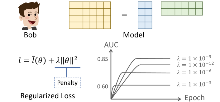
Figure 1. A motivating example of regularization tuning: the model is highly sensitive to the choice of $\lambda$.

The observation of high sensitivity to $\lambda$ motivates Bob to search for more fine-grained $\lambda$, as he believes that good $\lambda$ can substantially boost the performance. Instead of applying a uniform $\lambda$ on all embedding parameters, he considers varying it by the embedding dimensions. However, he has other tasks unfinished so he can’t babysit the tuning process. He decides to employ grid search with 10 candidate values. As the embedding size $K=128$, dimension-wise $\lambda$ would take about $10^{128}$ full training runs! So all Bob can do now is to buy new machines or babysit the tuning process by himself…

Examples similar to the above are not rare in industry. Practitioners like Bob, who often expect a high salary and a fantastic job with great intellectual challenges, would find their expectations clashing with the reality, spending most of the time on the tedious job of hyperparameter tuning. When it comes to recommender systems, tuning the regularization has been a nightmare for many practitioners whenever a new model is to be launched. Despite the high value of regularization tuning, there is relatively little research to conquer this issue. Methods like grid search could alleviate the laborious tuning process, but at a very high cost, especially when we want to tune $\lambda$ in a finer granularity. Other automated hyperparameter selection methods are also computation-expensive, since they typically require multiple full training runs (Shahriari et al., 2016; Snoek et al., 2012). An automatic method that can find appropriate $\lambda$ on the fly with affordable cost would be more than a blessing to practitioners.

Prior work on automatic regularization on recommender models is scarce. The most relevant method is SGDA(Rendle, 2012), which is a dimension-wise adaptive regularization method based on stochastic gradient descent (SGD). However, SGDA is designed for the task of rating prediction rather than personalized ranking, applying it would result in weak top-N recommendation performance (Cremonesi et al., 2010). In addition, we argue that more fine-grained $\lambda$, such as user-wise, is more advantageous than dimension-wise since it can adapt the regularization strength for users of different activity levels. Furthermore, adaptive optimizers like Adam (Kingma and Ba, 2015) and Adagrad (Duchi et al., 2011), are more effective and converge faster than SGD in optimizing recommender models (He and Chua, 2017). As such, we believe that there is an urgent need to develop an adaptive regularization method for top-K recommendation, and more importantly, should support fine-grained tuning with adaptive optimizers, instead of being merely applicable to dimension-wise tuning and plain SGD.

Contributions. In this paper, we explore how to design an automatic method to regularize recommender models. Focusing on the personalized ranking task (Rendle et al., 2009), we propose $\lambda$Opt, a generic regularizer that learns the regularization coefficients during model training based on validation data. The basic idea is to employ Bayesian Personalized Ranking (BPR) loss (Rendle et al., 2009) on validation data as the objective function, treating the regularization coefficients as the variable to the function and optimizing it with gradient descent. We illustrate our approach on matrix factorization, which is representative of a large family of embedding-based recommender models (Bayer et al., 2017). We highlight the elements that distinguish $\lambda$Opt as follows:

• $\lambda$Opt adaptively finds the appropriate $\lambda$. It enjoys substantially lower computation cost compared to other automated methods (Shahriari et al., 2016; Snoek et al., 2012) that require multiple training runs.

• By virtue of automatic differentiation, $\lambda$Opt obviates the complex derivations of gradients. Hence it can be conveniently generalized to a diverse set of recommender models.

• By permitting advanced optimizers with adaptive learning rates, $\lambda$Opt overcomes the issue of limited optimizer choice in (Rendle, 2012), making it more practitioner-friendly.

• Last but not least, our design of $\lambda$Opt facilitates regularization in any granularity. $\lambda$ can be dimension-wise, user-wise, item-wise or any combinations among them. Such fine-grained regularization brings considerable benefits to recommendation performance.

We conduct extensive experiments on $\lambda$Opt to justify its effectiveness in regularizing recommender models. We find that models trained with $\lambda$Opt significantly outperform grid search (fixed $\lambda$) and SGDA  (Rendle, 2012), demonstrating high utility of $\lambda$Opt. To sum up, $\lambda$Opt is a simple yet effective training tool, which not only lowers the barrier for practitioners to launch their recommender models but also boosts the performance with fine-grained regularization.

2. Preliminaries

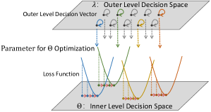
(a) Fixed approach

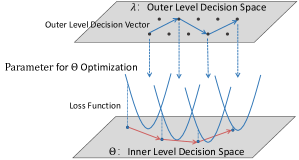
(b) Adaptive approach

Figure 2. $\Lambda$-trajectory for fixed regularization approach and adaptive regularization approach.

2.1. Matrix Factorization

Matrix Factorization (MF) (Koren et al., 2009) plays a dominant role in recommender systems. The basic principle behind MF is that we could project users or items into a latent space so that users’ preferences can be reflected using their proximity to the items. In spite of their prevalence, previous work on such matrix factorization models observes that the choice of the regularization coefficients $\lambda$ has significant influence on the trained models. Actually, this phenomenon stems from the inherent structure of matrix factorization models, — the number of parameters is often much larger than the number of samples, and the characteristics of recommendation datasets, – activity levels of users/items can be extremely diverse. Small $\lambda$ leads to overfitting while large $\lambda$ might cause underfitting. For this reason, it is no surprising that the problem of tuning regularization coefficients has been of extreme importance in practice.

2.2. Bayesian Personalized Ranking

Top-K item recommendation from implicit feedback is a prevalent task in real-world recommender systems (Chen et al., 2017; Yu et al., 2018; Zhang et al., 2017). With Bayesian Personalized Ranking (BPR) (Rendle et al., 2009) as the optimization objective, we study the adaptive regularization for factorization models. Targeting at learning from implicit feedback, BPR assumes that the user $u$ prefers the observed items over all the other unobserved ones. Formally, it aims to minimize the objective function:

(1) $$l_{S_{T}}(\Theta|\lambda) =\tilde{l}_{S_{T}}(\Theta)+\Omega(\Theta|\lambda)$$

(2) $$=-\sum_{(u,i,j)\in S_{T}}\ln(\sigma(\hat{y}_{ui}(\Theta)-\hat{y}_{uj}(\Theta)))+\Omega(\Theta|\lambda),$$

where $\Theta$ denotes the model parameters, $\lambda$ denotes the regularization coefficients, and $\sigma(\cdot)$ denotes the sigmoid function. $S_{T}=\{(u,i,j)|i\in\mathcal{I}_{u}\wedge j\in\mathcal{I}\backslash\mathcal{I}_{u}\}$ denotes the dataset of training triplets, where $\mathcal{I}_{u}$ represents the set of the observed items that user $u$ has interacted with in the past, and $\mathcal{I}$ denotes the set of all items. $\hat{y}_{ui}$ scores $(u,i)$ and can be parameterized using factorization models. $\Omega(\Theta|\lambda)$ is the penalty term indicating regularization on the model. Usually, the objective function is optimized by stochastic gradient descent (SGD). In addition to standard SGD optimizer, advanced optimizers that adapt their learning rate during training, for example, Adam (Kingma and Ba, 2015), can be used to accelerate the training process.

3. Methodology

In conventional regularization tuning, the goal is to find the optimal $\Lambda$ to train a regularized model, which achieves best performance on the validation set. Essentially, this can be formulated as a nested optimization problem (Rendle et al., 2009) or bi-level optimization problem (Sinha et al., 2018):

(3) $$\begin{split}\min_{\Lambda}\sum_{(u^{\prime},i^{\prime},j^{\prime})\in S_{V}}l(u^{\prime},i^{\prime},j^{\prime}|\arg\min_{\Theta}\sum_{(u,i,j)\in S_{T}}l(u,i,j|\Theta,\Lambda)),\end{split}$$

where the inner level attempts to minimize training loss with respect to $\Theta$ while the outer level addresses the minimization of validation loss with respect to $\Lambda$ on validation set $S_{V}$. A naive solution would be exhaustive search, training a regularized model for every possible $\Lambda$ and then choosing the one with the best validation performance. In practice, due to time and resources constraints, people resort to methods like grid-search, sampling $\Lambda$ from a small but reasonable interval. However, as model sizes and dataset volumes increase, grid search might also be unaffordable, particularly for large-scale applications, such as real-world recommendation.

In order to efficientize the search, previous work proposed to alternate the optimization of $\Lambda$ and $\Theta$, between consecutive full training runs (Chapelle et al., 2002; Larsen et al., 1998), or on the fly (Rendle, 2012; Luketina et al., 2016). Compared to grid-search, where $\Lambda$ is fixed during a full training run, the on-the-fly adaptive methods in (Rendle, 2012; Luketina et al., 2016) adjusts $\Lambda$ according to performance on validation sets every training step. Nevertheless, we show here that both approaches can be interpreted as attempting to find a plausible trajectory in the $\Lambda$ space to regularize the model well, and we introduce our proposed method later.

3.1. $\Lambda$-Trajectory

Definition 3.1.

A $\Lambda$-trajectory is the sequence of regularization coefficients for a full training run: $\Lambda=\{\Lambda_{1},...\Lambda_{T}\}$, where $T$ denotes the total steps in the training run.

Figure 2 visualizes $\Lambda$-trajectories for fixed approach and adaptive approach. In the nested optimization problem, there is an outer level decision space ($\Lambda$ space in our case) and an inner level decision space ($\Theta$ space in our case) (Sinha et al., 2018). Once $\Lambda$ is selected, it becomes a fixed parameter in the loss function for $\Theta$ optimization, indicated by the curve between the inner level decision space and outer level decision space in the figure. $\Lambda$-trajectories are represented using arrow lines in $\Lambda$ space with arrows indicating the update directions of $\Lambda$ at each training step.

3.1.1. Fixed $\Lambda$ Approach

In fixed $\Lambda$ approach, such as grid-search, we have the same regularization coefficients for all training steps, which are manually set at the beginning of training: $\Lambda_{1}=\Lambda_{2}=...=\Lambda_{T}$. Generally, grid-search goes as follows. We first select a few candidates from $\Lambda$ space. Then, we accordingly train multiple models and compare their performances on the validation set to choose the best $\Lambda$. The process can be regarded as trying out multiple $\Lambda$-trajectories while all of them are restricted – going around in circles as indicated in Figure 2(a). Due to the constraint on each $\Lambda$-trajectory, we usually need to search over a good number of $\Lambda$ candidates before $\Lambda$ space is explored sufficiently and appropriate regularization is achieved. The search either takes expensive computation or requires prior knowledge about picking suitable $\Lambda$ candidates. Even worse, if we consider regularization in finer levels, the computation of searching over all the selected $\Lambda$ would make grid-search barely feasible.

3.1.2. Adaptive $\Lambda$ Approach

As shown in Figure 2(b), the adaptive approach in (Rendle, 2012; Luketina et al., 2016), instead, employs different regularization coefficients at each training step, allowing faster exploration in $\Lambda$ space. We justify intuitions behind the adaptive approach here, which motivate us to adopt the adaptive paradigm when we design $\lambda$Opt.

• At different training stages, the strength of regularization should be different. For instance, there should be little regularization at the early stages of training since the model has not learned much from the data while strong regularization might be necessary for the late stage after the model sees the data a great many times.

• Assuming we have sufficient validation data, adjusting $\Lambda$ based on the validation performance would cause no obvious overfitting to the validation set.

• Although the resulted $\Lambda$-trajectory might not be optimal, it would be a competent one with substantially lower computation.

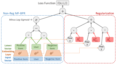
Figure 3. MF-BPR with Fine-grained Regularization.

3.2. $\lambda$Opt: Efficient Exploration over $\Lambda$ Space

In order to generate $\Lambda$-trajectories that steer efficient exploration over $\Lambda$ space, $\lambda$Opt takes into account the two aspects – $\Lambda$ in finer levels and its adaptive update. As we have just explained in Section 3.1, adaptive update of $\Lambda$ accelerates the exploration over $\Lambda$ space due to its flexibility in changing $\Lambda$ in a single training run. In this subsection, we show how fine-grained $\Lambda$ contributes to the exploration and present $\lambda$Opt formally.

3.2.1. Recommender Models with Fine-grained Regularization

As shown in Figure 3, traditional matrix factorization with BPR (MF-BPR) consists of a non-regularized block and a regularized block. Distinguished from common regularization strategies, setting a global $\lambda$ or dimension-wise $\lambda$, we consider regularization in finer levels – the regularized part in our method is user-/item-aware instead of being only dimension-wise. Given the fact that recommender systems interact with heterogeneous users and items, incorporating user-/item-aware regularization into $\lambda$Opt can be vital. Besides, from the perspective of $\Lambda$-trajectories, entailing the same regularization for each user/item, dimension-wise $\lambda$ or global $\lambda$ equivalently forbids exploration in directions related to users/items, thus preventing the discovery of better regularization strategies to train recommender models.

3.2.2. Regularizer Endowed with Adaptive Regularization in Finer Levels

In this subsection, we show how we derive the adaptive update of $\Lambda$ in our method. We choose to implement $\lambda$Opt as neural networks with $\Lambda$ as weights. Such design is more practitioner-friendly compared to SGDA, since it saves them from complex derivations of the gradients and makes $\lambda$Opt easy to generalize across various models, loss functions and model optimizers.

The nested optimization problem in Equation 3 is hard to solve directly. Alternating optimization (Rendle, 2012) reduces it into two simpler ones. To be exact, we perform the following two steps iteratively

• $\Theta$ Update at Step t. We fix $\Lambda_{t}$ while $\Theta$ is optimized using triplets $(u,i,j)$ sampled from train set $S_{T}$. Notice that we employ $\Lambda$ in finer levels to compute the regularized training loss.

• $\Lambda$ Update at Step t. We fix $\Theta_{t}$ while $\Lambda$ is computed by optimizing the expected validation loss with triplets $(u,i,j)$ sampled from validation set $S_{V}$.

Since our goal is to find $\Lambda$ which would achieve the smallest validation loss, we need to figure out the relationship between $\Lambda$ and the validation loss. As pointed out in (Rendle, 2012), while the validation loss for current model $l_{S_{V}}(\Theta_{t})$ has nothing to do with $\Lambda_{t}$, the expected validation loss $l_{S_{V}}(\Theta_{t+1})$ instead depends on $\Lambda_{t}$ if $\Theta_{t+1}$ is obtained using $\Lambda_{t}$. This suggests that we can first obtain the assumed next-step model parameters $\bar{\Theta}_{t+1}$ and then compute the validation loss with $\bar{\Theta}_{t+1}$ and its gradients with respect to $\Lambda$. We use the word ”assumed” because this update is never really performed on the model we finally want. We only use it to obtain the direction to update $\Lambda$ i.e. to move a step in $\Lambda$-trajectory. We use symbols in the format of $\bar{\cdot}$ to distinguish ”assumed” ones from ordinary ones.

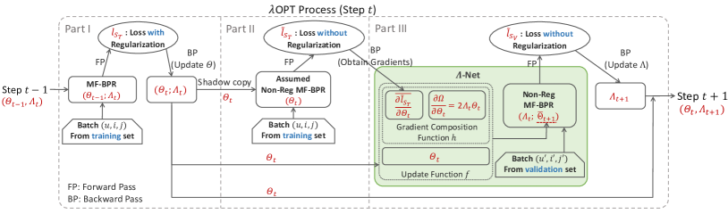
Figure 4. Regularizer Endowed with Adaptive Regularization in Finer Levels.

Obtain Assumed Next-Step Model Parameters $\bar{\Theta}_{t+1}$.

The key to obtain $\bar{\Theta}_{t+1}$ is to compute the gradients of assumed regularized training loss with respect to $\Theta_{t}$. $\lambda$Opt tackles this via splitting the gradients into two terms, one for non-regularized loss and the other for the penalty term:

(4) $$\overline{\frac{\partial{l_{S_{T}}}}{\partial\Theta_{t}}}=h(\overline{\frac{\partial\tilde{l}_{S_{T}}}{\partial\Theta_{t}}},\Theta_{t})=\overline{\frac{\partial\tilde{l}_{S_{T}}}{\partial\Theta_{t}}}+\frac{\partial\Omega}{\Theta_{t}}.$$

We denote as $h$ the function composing non-regularized gradients and regularized gradients. In fine-grained $L_{2}$ regularization, $\Omega(\Theta|\Lambda)=\Lambda||\Theta||_{2}^{2}$, Equation 4 would be

(5) $$\overline{\frac{\partial{l_{S_{T}}}}{\partial\Theta_{t}}}=h(\overline{\frac{\partial\tilde{l}_{S_{T}}}{\partial\Theta_{t}}},\Theta_{t})=\overline{\frac{\partial\tilde{l}_{S_{T}}}{\partial\Theta_{t}}}+2\Lambda\Theta_{t}.$$

As we don’t want assumed gradients to mess around with the ones in MF-BPR, $\lambda$Opt performs a separate forward & backward computation on $S_{T}$ to obtain $\overline{\frac{\partial\tilde{l}_{S_{T}}}{\partial\Theta_{t}}}$ as illustrated in Part II of Figure 4. After composition of assumed regularized gradients using $h$, the assumed next-step model parameters are given by $\bar{\Theta}_{t+1}=f(\Theta_{t},\overline{\frac{\partial l_{S_{T}}}{\partial\Theta_{t}}})$ where $f$ is the update function of $\Theta$, generally determined by the optimizer $\Theta$ update used.

Minimize the Validation Loss

Up to now, we have obtained assumed next-step model parameters $\bar{\Theta}_{t+1}$ and the only remaining job is to find the $\Lambda$ which minimizes validation loss $l_{S_{V}}(\bar{\Theta}_{t+1})$. Note that this is a constrained minimization though treated as unconstrained in SGDA (Rendle, 2012). Mathematically, we want to solve

(6) $$\begin{split}\arg\min_{\Lambda}-\sum_{(u,i,j)\in S_{V}}\ln(\sigma(\hat{y}_{ui}(\bar{\Theta}_{t+1})-\hat{y}_{uj}(\bar{\Theta}_{t+1})),\\ \text{subject to }\Lambda\geq 0.\\ \end{split}$$

Karush-Kuhn-Tucker (KKT) conditions for constrained minimization with non-convex objectives give feasible regions in $\Lambda$ space, which make the search more efficient and stable. The gradients of validation loss with respect to $\Lambda$ are denoted as $G$

(7) $$G=\nabla_{\Lambda}-\sum_{(u,i,j)\in S_{V}}\ln(\sigma(\hat{y}_{ui}(\bar{\Theta}_{t+1})-\hat{y}_{uj}(\bar{\Theta}_{t+1})).$$

Then KKT gives

(8) $$\Lambda G=0,G\geq 0,\Lambda\geq 0.$$

From Equations 8, we can see that feasible solutions of $\Lambda$ require both $G$ and $\Lambda$ to be non-negative with one of them equals to zero. A slack version could be encouraging $G$ to be small and $\Lambda$ to be non-negative.

Part III of Figure 4 shows the computation flow of minimizing validation loss in $\lambda$Opt. We term the entire block in green colour as $\Lambda$-Net because the parameters here are $\Lambda$ rather than $\Theta$. After forward & backward passes over $\Lambda$-Net, we add the slack constraints given by Equation 8: clip the gradients $G$ to a small value and smooth the negative entries in $\Lambda$ as zero. The updated parameters of $\Lambda$-Net serve as the regularization coefficients $\Lambda_{t+1}$ for MF-BPR in next iteration.

Computation Cost

$\lambda$Opt adjusts $\Lambda$ on the fly, which obviates multiple full training runs as grid-search like methods. Since one iteration takes 3 forward passes and backpropagations, the computation cost for a single training run is only 3 times the one for the fixed approach. For practitioners, this is cost-effective because they do not have to search over a great many of $\Lambda$ candidates.

4. Applications

In this section, we show how to apply $\lambda$Opt with various model optimizers and fine-grained regularization. We start from the simple matrix factorization model. Generally, the model parameters, user embedding $\Theta^{U}$ and item embedding $\Theta^{I}$, should be matrices of $|U|\times K$ and $|I|\times K$ respectively, where $K$ stands for number of dimensions. As stated above, we only need to specify the forward pass for the model and optimizer update. For MF, the forward pass to compute non-reg BPR loss is

(9) $$\tilde{l}(u,i,j,\Theta|\Lambda)=-ln(\sigma(\Theta^{U}_{u}\cdot\Theta^{I}_{i}-\Theta^{U}_{u}\cdot\Theta^{I}_{j})).$$

The model parameters are $\Theta=\{\Theta^{U},\Theta^{I}\}$. Correspondingly, the regularization coefficients are $\Lambda=\{\Lambda^{U},\Lambda^{I}\}$.

4.1. Optimizer Choices

When training recommender models, various optimizers can be used. Model parameters update of these optimizers are often different. Unlike SGDA (Rendle, 2012) and (Luketina et al., 2016), $\lambda$Opt can cope with various optimizers as long as the model parameter update function $f$ is derivable with respect to $\Lambda$. For example, if we use a SGD optimizer,

(10) $$\bar{\Theta}_{t+1}=f(\Theta_{t},\overline{\frac{\partial l_{S_{T}}}{\partial\Theta_{t}}})=\Theta_{t}-\eta h(\overline{\frac{\partial{l}_{S_{T}}}{\partial\Theta_{t}}},\Theta_{t}).$$

Substituting Equation 4 and Equation 5 into the above equation, we can obtain

(11) $$\bar{\Theta}_{t+1} =f(\Theta_{t},\overline{\frac{\partial l_{S_{T}}}{\partial\Theta_{t}}})=\Theta_{t}-\eta\overline{\frac{\partial\tilde{l}_{S_{T}}}{\partial\Theta_{t}}}-2\eta\Lambda\Theta_{t}.$$

In order to obtain the validation loss’s gradient with respect to $\Lambda$, we need to compute $\frac{\partial f}{\partial\Lambda}$. For the simple SGD optimizer, this would be easy: $-2\eta\Theta_{t}$. However, it is not the case for complex optimizer like Adam, which is among the off-the-shelf choices when practitioners start to train their factorization models — they would have to derive the gradients themselves! Luckily, in $\lambda$Opt, this step of obtaining gradients would be handled by Automatic Differentiation framework such as TensorFlow (Abadi et al., 2016) and PyTorch. Hence, we don’t need to worried about the complex derivation of $\frac{\partial f}{\partial\Lambda}$. For Adam optimizer, we only need to specify $f$ as follows:

(12) $$\bar{\Theta}_{t+1} =\Theta_{t}-\eta\frac{\sqrt{1-\beta_{2}^{t}}}{\sqrt{1-\beta_{1}^{t}}}\frac{s_{t}}{\sqrt{r_{t}}+\epsilon},$$

(13) $$s_{t} =\beta_{1}s_{t-1}+(1-\beta_{1})\overline{\frac{\partial l_{S_{T}}}{\partial\Theta_{t}}},$$

(14) $$r_{t} =\beta_{1}r_{t-1}+(1-\beta_{1})\overline{\frac{\partial{l_{S_{T}}}}{\partial\Theta_{t}}}\odot\overline{\frac{\partial{l_{S_{T}}}}{\partial\Theta_{t}}}.$$

4.2. Fine-grained Regularization

To our knowledge, no previous work has explored regularization in finer levels, like user-/item-aware regularization. Grid-search fails due to unaffordable computation cost of searching over extremely high-dimensional $\Lambda$ spaces. And SGDA is also not applicable since its derivation only considers dimension-aware regularization but does not adapt with users and items. As stated in Section 3.2.1, our design of $\lambda$Opt naturally lends itself to user/item-aware $\Lambda$. Fine-grained regularization, for example user-wise regularization, could be done by expanding the penalty term and obtaining the gradients as following:

(15) $$\Omega(\Theta^{U},\Theta^{I}|\Lambda^{U},\lambda^{I}) =\sum_{u=1}^{|U|}\Lambda^{U}_{u}\sum_{k=1}^{K}(\Theta^{U}_{u,k})^{2}+\lambda^{I}||\Theta^{I}||_{2}^{2},$$

(16) $$\frac{\partial\Omega}{\partial\Theta^{U}_{u,k}} =2\Lambda_{u}^{U}\Theta_{u,k}^{U},\frac{\partial\Omega}{\partial\Theta^{I}}=2\lambda^{I}\Theta^{I},$$

where $\Lambda^{U}$ is a $|U|\times 1$ vector specifying the user-wise regularization for the user embedding matrix and $\Lambda^{I}$ is a scalar specifying the regularization for item embedding matrix. Similarly, we can use more fine-grained regularization $\Lambda$ that combines dimension-wise, user-wise and item-wise.

(17) $$\!\!\!\!\!\Omega(\Theta^{U},\Theta^{I}|\Lambda^{U},\Lambda^{I})\!=\!\!\sum_{u=1}^{|U|}\!\sum_{k=1}^{K}\!\Lambda^{U}_{u,k}(\Theta_{u,k}^{U})^{2}\!+\!\sum_{i=1}^{|I|}\!\sum_{k=1}^{K}\Lambda^{I}_{i,k}(\Theta_{i,k}^{I})^{2},$$

(18) $$\frac{\partial\Omega}{\partial\Theta^{U}_{u,k}}=2\Lambda_{u,k}^{U}\Theta_{u,k}^{U},~{}~{}~{}~{}~{}\frac{\partial\Omega}{\partial\Theta^{I}_{i,k}}=2\Lambda_{i,k}^{I}\Theta_{i,k}^{I},$$

where $\Lambda^{U}$ and $\Lambda^{I}$ are $|U|\times K$ and $|I|\times K$ matrices respectively.

5. Empirical Study

In this section, we empirically evaluate our methods with the aim of answering the following research questions:

• What is the performance of MF models trained using $\lambda$Opt? The adaptive method can save practitioners a lot time. But does it come at a cost of worse performance compared to other regularization strategies?

• With $\lambda$Opt, practitioners can add fine-grained regularization over MF models conveniently, which is infeasible in grid-search like methods. Will such fine-grained regularization be effective in addressing heterogeneous users and items?

• What are the $\Lambda$ trajectories of $\lambda$Opt like? Does $\lambda$Opt find better trajectories to regularize the model? The $\Lambda$ trajectories can explain the performance difference across users and items with varied frequency, telling us why $\lambda$Opt performs better or worse than the fixed approaches.

5.1. Experimental Settings

5.1.1. Datasets

We experiment with two public datasets: Amazon Food and MovieLens 10M. Table 1 summarizes the statistics of datasets after pre-processing.

- Amazon Food Review. It contains reviews of fine foods from amazon, spanning a period of more than 10 years. We filter the dataset and only keep the users and items with more than 20 records. We omit the exact scores and treat every entry in the dataset as a positive sample.

- MovieLens 10M. It is a widely used benchmark dataset and contains timestamped user-movie ratings ranging from $1$ to $5$. We use the “10M” version, which contains approximately $10$ million ratings drawn from 69,878 users. Each user has at least 20 ratings. We use it as an implicit feedback dataset, where the exact ratings are omitted and each entry is regarded as a positive sample.

Table 1. Statistics of datasets.

Dataset	# User	# Item	# Interaction	Density
Amazon Food	$1,238$	$3,806$	$38,919$	$0.825\%$
MovieLens 10M	$69,878$	$10,677$	$10,000,054$	$1.340\%$

5.1.2. Performance Measures

For both Amazon Food Review and MovieLens 10M, we divide the data according to the time stamp information. Specially, for each user, all the records are divided into training, validation and testing set based on the proportion $60\%$, $20\%$ and $20\%$. To evaluate the performance of our methods, for each (user, item) pair in the test set, we make recommendations by ranking all the items that are not interacted by the user in the training and validation set. Three metrics are evaluated:

- AUC. Area under the Receiver Operating Characteristic or ROC curve (AUC) means the probability to rank a randomly chosen positive item higher than a randomly chosen negative item.

- HR. Hit Ratio (HR) is based on recall. It intuitively measures whether the test item is in the top-K list. We set K, the truncation length of the ranking list, to be $50$ (HR@50) and $100$ (HR@100).

- NDCG. Normalized Discounted Cumulative Gain (NDCG) considers positions of hits in the top-K list, where hits at higher positions get higher scores. K is as stated above.

For HR and NDCG, we report the average score of all the users. The score for each user is averaged over all his/her test items. For all the metrics, higher score is better.

Table 2. Recommendation Performance on Amazon Food Review and MovieLens 10M.

Method		Amazon Food Review					MovieLens 10M
		AUC	​HR@50	​HR@100	​NDCG@50	​NDCG@100	AUC	​HR@50	​HR@100	​NDCG@50	​NDCG@100
SGDA (Rendle, 2012)		0.8130	0.1786	0.3857	0.1002	0.1413	0.9497	0.2401	0.3706	0.0715	0.0934
AMF (He et al., 2018)		0.8197	0.3541	0.4200	0.2646	0.2552	0.9495	0.2625	0.3847	0.0787	0.0985
NeuMF (He et al., 2017)		0.8103	0.3537	0.4127	0.2481	0.2218	0.9435	0.2524	0.3507	0.0760	0.0865
MF-$\lambda$Fix		0.8052	0.3482	0.4163	0.2251	0.2217	0.9497	0.2487	0.3779	0.0727	0.0943
MF-$\lambda$Opt	-D​	0.8109	0.2134	0.3910	0.1292	0.1543	0.9501	0.2365	0.3556	0.0715	0.0909
	-DU	0.8200	0.3694	0.4814	0.2049	0.2570	0.9554	0.2743	0.4109	0.0809	0.1031
	-DI	0.8501	0.2966	0.4476	0.1642	0.2039	0.9516	0.2648	0.3952	0.0804	0.1013
	-DUI	0.8743	0.4470	0.5251	0.2946	0.2920	0.9575	0.3027	0.4367	0.0942	0.1158

5.1.3. Baselines

We compare our methods with the following state-of-the-art methods:

-MF-$\lambda$Fix. For the fixed regularization methods, we use a global $\lambda$ for all latent dimensions, users and items due to limited computation resources. To simulate how the practitioner would select the best $\lambda$, we searched for the best $\lambda$ among $\{10,1,10^{-1}\!,10^{-2}\!,10^{-3}\!,10^{-4},$ $10^{-5},0\}$. For each $\lambda$, we ran a full training of the model and checked its performance on the validation set. The best one is selected for comparison with the model trained by our $\lambda$Opt regularizer.

- SGDA (Rendle, 2012). As mentioned in Section 1, SGDA is an adaptive regularization method based on dimension-wise regularization and SGD, derived for rating prediction task. For top-K recommendation, we have to re-derive it by hand. Luckily, it can be roughly seen as $\lambda$Opt with dimension-wise $\Lambda$ and SGD for MF updates. We find that the implanted SGDA can be very hard to tune due to its limitation in optimizer choices. As SGD doesn’t adjust the learning rate during training, the initial learning rate is crucial to the final performance. Meanwhile, it is pretty hard to tune the learning rate for SGD as small learning rate leads to slow convergence and large learning rate might contribute to bad performance. Here we follow the same tuning flow as we tune the models for our approach. We first find an appropriate learning rate for the fixed SGD MF. And then we add the SGDA regularizer to the SGD MF with this learning rate and tune the hyperparameters for the SGDA regularizer.

- AMF (He et al., 2018). Adversarial Matrix Factorization (AMF) is a state-of-the-art model for recommendation. It employs Adversarial Personalized Ranking (APR) method, which enhances vanilla MF by performing adversarial training. In our experiments, we start adversarial training when the loss of MF-$\lambda$Fix converges and tune the learning rate and $L_{2}$ regularizer, as described in the paper.

- NeuMF (He et al., 2017). Neural Matrix Factorization (NeuMF) is a state-of-the-art neural model for item recommendation, combining MF and Multi-Layer Perceptrons (MLP) to learn user-item interaction. Following (He et al., 2017), we first pretrain the model with MF-$\lambda$Fix, and then tune the depth of MLP, learning rate, and $L_{2}$ regularization.

As for our method, we adopt Adam as the optimizer for MF update. The reason is that, in our experiments, we find the training of recommender models with adaptive regularizers is much more sensitive to the step sizes compared to training with the fixed regularizer. Practitioners of such methods could be eager for optimizers that adapt their learning rates during the training procedure of recommender models. Since SGDA only gives $\lambda$-update solutions to the models optimized by vanilla SGD, our method is more generic in terms of endowing the practitioners more freedom in optimizer choices. For fair comparison, we use the same MF model configurations for MF-$\lambda$Fix, SGDA, AMF and $\lambda$Opt as we want to justify the effect of various regularization strategies.

5.2. Performance of $\lambda$Opt (RQ.1)

Table 2 shows the results. Our methods are named as ”MF-$\lambda$Opt-[regularization granularity]”, with “D”, “U”, “I” and “DUI” standing for dimension-wise, user-wise, item-wise and the three respectively. On both datasets, MF-$\lambda$Opt-DUI outperforms the other methods by a large margin – about 10%-20% in HR and NDCG. The variants of $\lambda$Opt with different regularization granularity also show promising performance, which indicates that $\lambda$Opt lowers down the computation barrier and prerequisite for practitioners without hurting model performance. In fact, it even boosts the recommendation performance if combined with suitable fine-grained regularization.

5.3. Sparseness and Activeness (RQ.2)

Section 5.2 demonstrates $\lambda$Opt’s superiority over others. But where does $\lambda$Opt gain its performance improvements? Do they come from handling the sparse users better than the fixed $\lambda$ approach? Or do they come from addressing active users better? In order to validate $\lambda$Opt’s, to be exact, MF-$\lambda$Opt-DUI’s effectiveness in addressing heterogeneous users/items, we check its performance improvements across users/items with varied frequencies. Due to limited space, we only present figures on Amazon Food Review Dataset. The results on MovieLens 10M are similar.

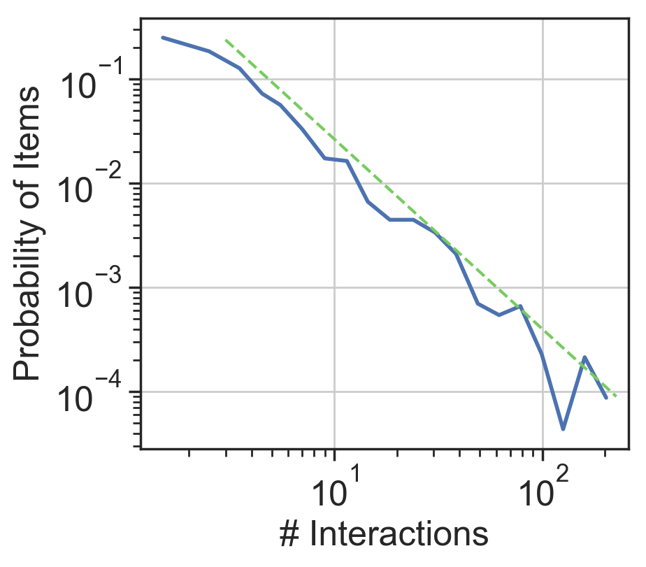
(a) Users on Amazon Food Review

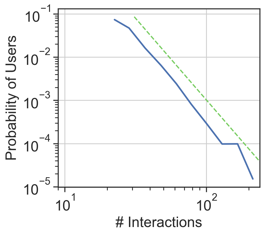
(b) Items on Amazon Food Review

Figure 5. Distributions of user and item frequencies.

Figure 5 shows the distributions of user and item frequencies on Amazon Food Review. We can observe that they are all long-tailed. This poses a great challenge to the recommender model, as it needs to be flexible enough to take care of both the head users/items (sparse) and tail users/items (active). Regularization strategies that set a global $\lambda$ or dimension-wise $\lambda$ for all users/items might not work well as they cannot address both types of users. Choosing an appropriate $\lambda$ via grid-search, in essence, seeks compromise between sparse and active users/items. In contrast, regularization in finer levels, e.g. user-/item-aware regularization, obviates the need to compromise between users/items with diverse frequencies.

MF-$\lambda$Opt-DUI specifies an individual level of regularization strength for each user, item and dimension. We investigate its impact on users/items with varied numbers of interactions. Figure 6 shows its performance improvements (HR@100 and NDCG@100) over the fixed approach on Amazon Food Review. The HR and NDCG for users are defined as stated in the experimental settings. For an item, as it is not convenient to compute item-wise measures in BPR setting, we compute its ”HR” and ”NDCG” as follows: In the test set, we find the users that interact with the item and take the average of their HRs as the ”HR” for the item; we find the users that interact with the item and take the average of their NDCGs as the ”NDCG” for the item. Such measures are useful in making comparisons across different methods.

As we can observe from Figure 6, except ¡15 item group, MF-$\lambda$Opt-DUI lifts performances by about $10\%$ across users/items in varied frequency groups, conforming to our design that $\lambda$Opt can handle both sparseness and activeness better.

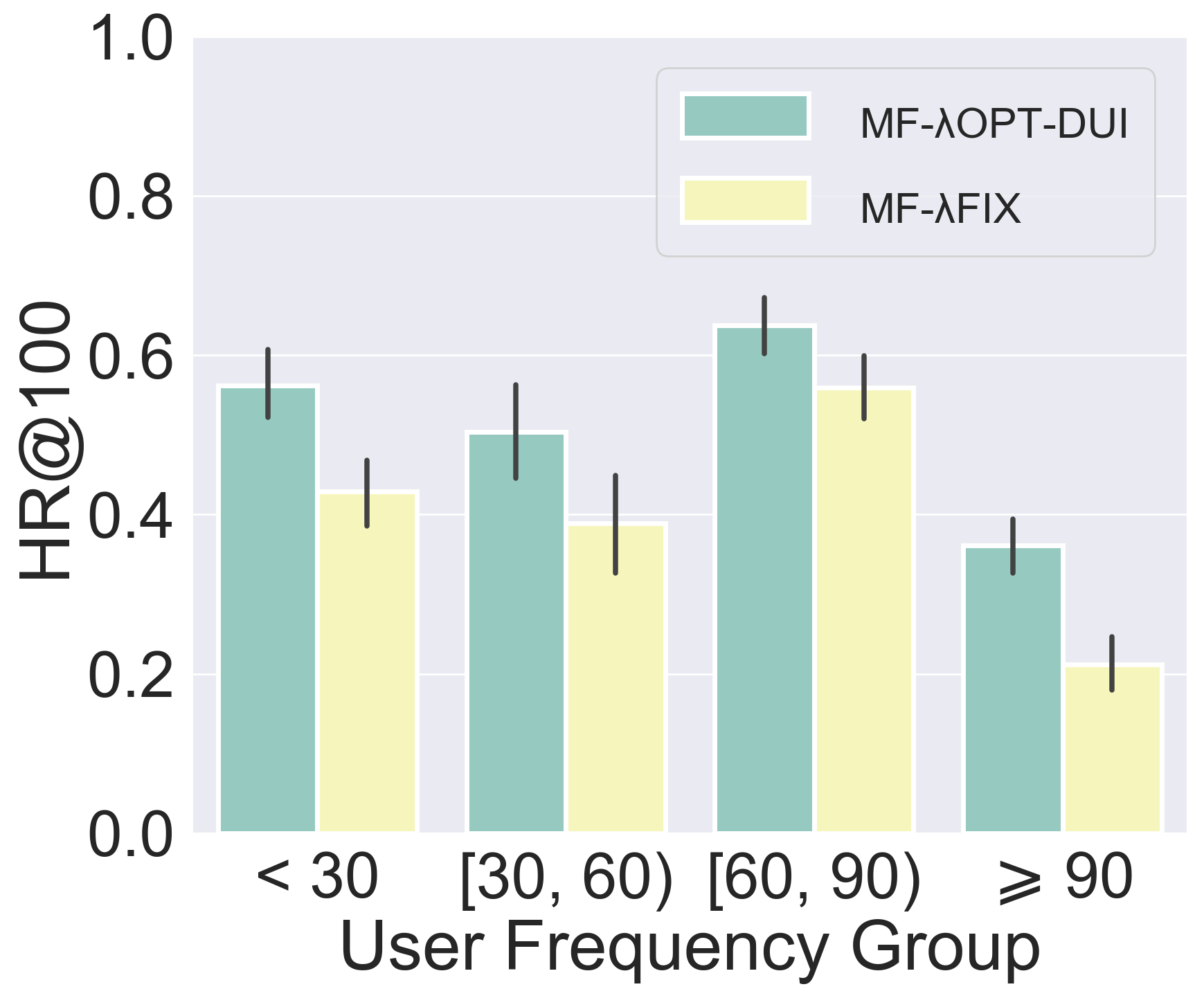
(a) HR@100 for users

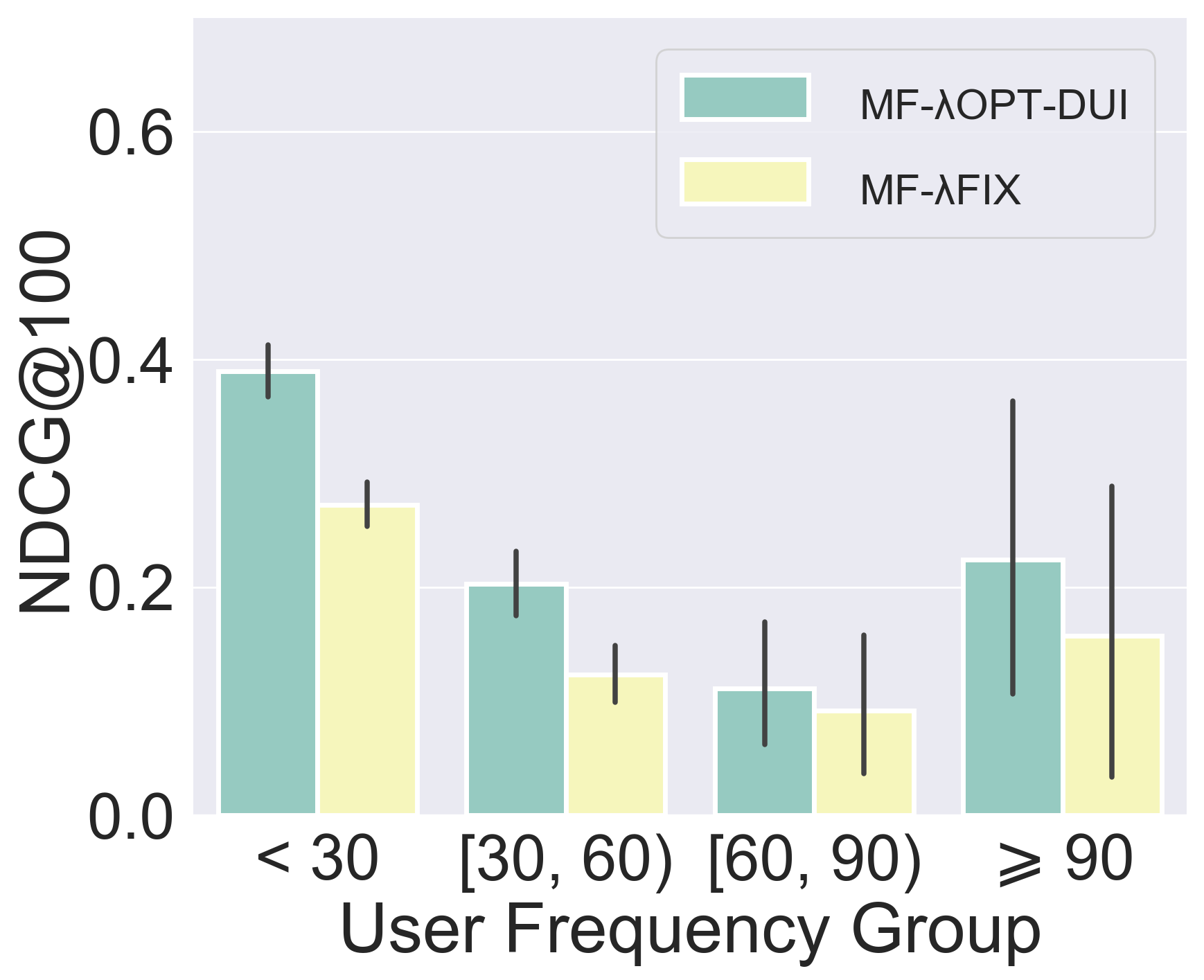
(b) NDCG@100 for users

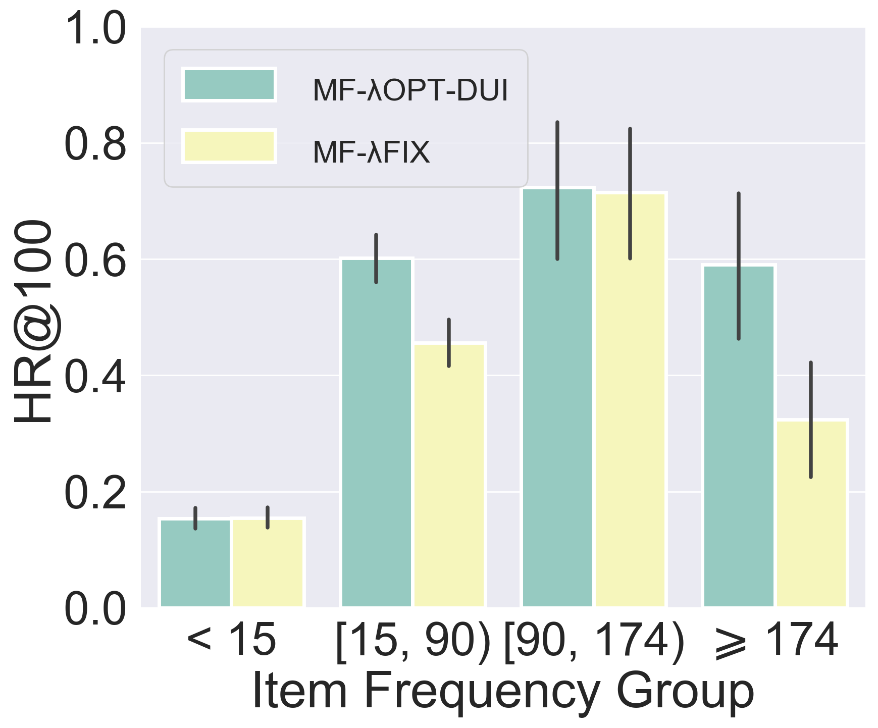
(c) HR@100 for items

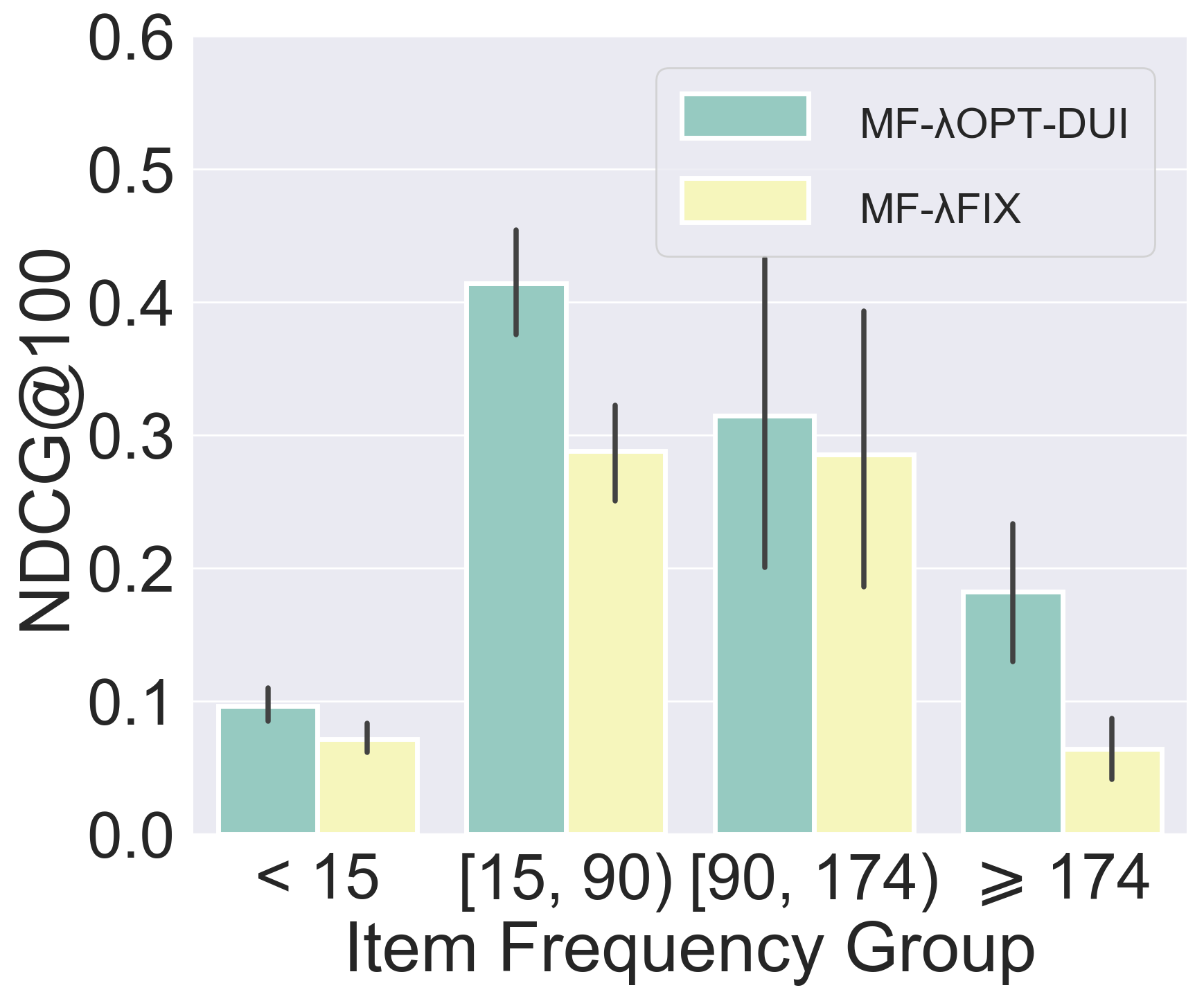
(d) NDCG@100 for items

Figure 6. Performance improvements of users/items in varied frequency groups on Amazon Food Review.

5.4. Analysis of $\Lambda$-trajectories (RQ.3)

How does $\lambda$Opt adjust $\lambda$ to gain such surprising improvement across heterogeneous users and items? In other words, does $\lambda$Opt find special $\Lambda$-trajectories for them? We dive into this research question by analyzing the $\Lambda$-trajectories.

Figure 7 shows the $\Lambda$-trajectories. Different colors indicate different groups of users and items divided according to numbers of interactions. For every user and item, we aggregate the $\Lambda$ over all the latent dimensions. We then take the average of all users or items within the same group. The variance within a group is indicated by the shades in the figure. Figure 8 shows the relationship between $\lambda$ and the frequency for users/items, evolving as training epoch increases. Color implies the magnitudes of $\lambda$.

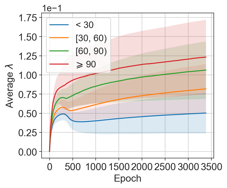
(a) For users on Amazon Food Review

(b) For items on Amazon Food Review

Figure 7. $\Lambda$-trajectories generated by MF-$\lambda$Opt-DUI.

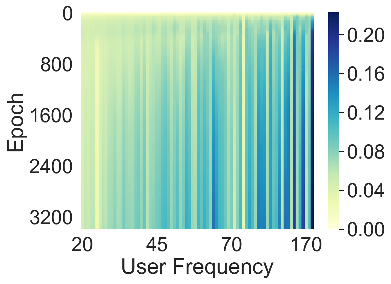
(a) For users on Amazon Food Review

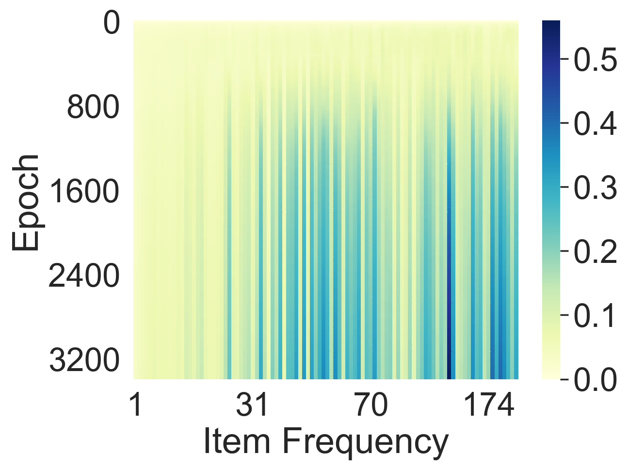
(b) For items on Amazon Food Review

Figure 8. Relationship between frequencies and average $\lambda$ by MF-$\lambda$Opt-DUI, evolving as training epoch increases. Color indicates the magnitude of average $\lambda$.

As we could see, most $\lambda$s tend to increase as the training procedure goes on. This conforms to the intuition that regularization is necessary after the model encounters the data multiple times. Difference among groups can also be observed. Interestingly, the active users receive stronger regularization after epochs of training although the initial $\Lambda$ is zero for all users. A possible explanation would be the active users have more data and the model learns from the data so quickly that it might get overfitting to them, making strong regularization necessary. Under these circumstances, a global strong regularization level would satisfy the active users but at the risk of failing the sparse users. In contrast, $\lambda$Opt finds a special $\Lambda$-trajectory for every user, being capable to please both sparse users and active users. As shown in Figure 7, sparse users receive a relatively weak regularization so that recommendation to them could rely more on the data. The findings on the item $\Lambda$-trajectories are similar. We could conclude here that $\lambda$Opt owns most of its improvements to finding ”personalized” $\Lambda$-trajectories for a diverse set of users and items. We believe this property is valuable to most large-scale web applications where long-tailed phenomenons are common and data sparsity remains a severe challenge.

So far, we have justified that $\lambda$Opt not only lowers down the computation cost needed to search for a good regularization level but also has the potential to boost the recommendation performance by fine-grained regularization. We also reveal its secret in improving the recommendation performance by analyzing the $\Lambda$-trajectories.

6. Related Work

Adaptive Regularization for Rating Prediction.

The close work is SGDA (Rendle, 2012), where adaptive regularization for rating prediction is achieved by alternating optimization for model parameters $\Theta$ and regularization coefficients $\lambda$. Similar validation set based alternating optimization method has also been proposed in (Luketina et al., 2016). Both work focused on the reduced computation complexity while ignoring the potential performance boost. As far as we know, we are the first to reveal the important insight that, adaptive regularization in finer levels can bring additional performance benefits for recommender systems. (Rendle, 2012) only considers dimension-wise $\lambda$, which might be the reason why the algorithm does not outperform the best fixed $\lambda$ algorithm in the reported experimental results. Instead, our work shows the effectiveness of incorporating fine-grained regularization. Besides, our method is more generic in terms of endowing the practitioners more freedom in optimizer choices while SGDA(Rendle, 2012) applies only to SGD optimizers.

Hyperparameters Optimization.

Finding good regularization coefficients can be part of the overall hyperparameters optimization (HO). Typically, grid-search-like methods are used where people monitor performance on the validation set and choose the best set of hyperparameters from a bunch of candidates. These methods are simple and generic, capable of being applied to any task and any model, ranging from SVM (Hsu et al., 2003) to decision trees. Random search could be very time-consuming. Previous work (Snoek et al., 2012; Shahriari et al., 2016; Snoek et al., 2015; Li et al., 2016; Feurer et al., 2014) have dedicated to lower down the nontrivial search cost, along with developing some enhanced toolboxes (Martinez-Cantin, 2014; Bergstra et al., 2013; Claesen et al., 2014). However, most of them require multiple full training runs instead of learning to regularize on the fly. Recently, (Franceschi et al., 2018) explored bilevel programming to unify gradient based HO and meta-learning. The above hyper-parameters optimization methods do not specialize on recommender systems. Applying them to tuning the regularization coefficients for recommendation might not work well due to some characteristics, i.e., data sparsity issue, in recommender systems. In contrast, our algorithms are tailored to recommendation, where users/items are highly heterogeneous.

Regularization of Embeddings.

Embedding technique is widely used to project categorical values into a latent vector space (Guo and Berkhahn, 2016). In natural language processing, training large embeddings usually requires suitable regularization (Peng et al., 2015). Training recommender models also involves regularizing large embedding matrices, such as the user/item embedding matrix. Although the tasks are different, the basic regularization strategies and their analysis might be similar. A cross-sectional study across them would be interesting and meaningful in terms of deriving a generic regularization method for embeddings. Since parameters initialization can be regarded as a special regularization, embedding initialization methods like (Pan et al., 2019) are also worth exploring.

7. Conclusion and Future Work

Tuning regularization hyperparameters for recommender models has been a tedious even miserable job for practitioners. We propose a generic method, $\lambda$Opt, to address this problem. $\lambda$Opt adjusts the regularization hyperparameters on the fly based on validation data. Our experiments based on two benchmarks demonstrate that $\lambda$Opt can be a simple yet effective training tool in terms of lower computation cost and better performance with fine-grained regularization.

In future, we are interested in extending our method to more complex models, such as FM and NeuMF. Since $\lambda$Opt relies on validation data to update the regularization coefficients, it requires sufficient data to ensure the generalization (Rendle, 2012; Snoek et al., 2015) when the number of hyperparameters is large. It would be worthwhile to investigate the influence of validation data size. Moreover, we would like to dive into the theoretical foundation for such adaptive hyperparameter optimization methods, which is significant for further applications.

- (1)
- Abadi et al. (2016) Martín Abadi, Paul Barham, Jianmin Chen, Zhifeng Chen, Andy Davis, Jeffrey Dean, Matthieu Devin, Sanjay Ghemawat, Geoffrey Irving, Michael Isard, et al. 2016. Tensorflow: a system for large-scale machine learning.
- Agarwal and Chen (2011) Deepak Agarwal and Bee-Chung Chen. 2011. Machine Learning for Large Scale Recommender Systems. http://pages.cs.wisc.edu/~beechung/icml11-tutorial/.
- Bayer et al. (2017) Immanuel Bayer, Xiangnan He, Bhargav Kanagal, and Steffen Rendle. 2017. A generic coordinate descent framework for learning from implicit feedback. In WWW.
- Bergstra et al. (2013) James Bergstra, Dan Yamins, and David D Cox. 2013. Hyperopt: A python library for optimizing the hyperparameters of machine learning algorithms. In Python in Science Conference. 13–20.
- Chapelle et al. (2002) Olivier Chapelle, Vladimir Vapnik, Olivier Bousquet, and Sayan Mukherjee. 2002. Choosing multiple parameters for support vector machines. Machine learning 46, 1-3 (2002), 131–159.
- Chen et al. (2017) Jingyuan Chen, Hanwang Zhang, Xiangnan He, Liqiang Nie, Wei Liu, and Tat-Seng Chua. 2017. Attentive collaborative filtering: Multimedia recommendation with item-and component-level attention. In SIGIR.
- Claesen et al. (2014) Marc Claesen, Jaak Simm, Dusan Popovic, Yves Moreau, and Bart De Moor. 2014. Easy hyperparameter search using Optunity. arXiv:1412.1114 (2014).
- Cremonesi et al. (2010) Paolo Cremonesi, Yehuda Koren, and Roberto Turrin. 2010. Performance of Recommender Algorithms on Top-n Recommendation Tasks. In RecSys.
- Duchi et al. (2011) John Duchi, Elad Hazan, and Yoram Singer. 2011. Adaptive subgradient methods for online learning and stochastic optimization. JMLR 12, Jul (2011), 2121–2159.
- Dyer et al. (2011) Justin S Dyer, Art B Owen, et al. 2011. Visualizing bivariate long-tailed data. Electronic Journal of Statistics 5 (2011), 642–668.
- Feurer et al. (2014) Matthias Feurer, Jost Tobias Springenberg, and Frank Hutter. 2014. Using meta-learning to initialize bayesian optimization of hyperparameters. In International Conference on Meta-learning and Algorithm Selection.
- Franceschi et al. (2018) Luca Franceschi, Paolo Frasconi, Saverio Salzo, Riccardo Grazzi, and Massimiliano Pontil. 2018. Bilevel Programming for Hyperparameter Optimization and Meta-Learning. In International Conference on Machine Learning. 1563–1572.
- Guo and Berkhahn (2016) Cheng Guo and Felix Berkhahn. 2016. Entity embeddings of categorical variables. arXiv:1604.06737 (2016).
- He and Chua (2017) Xiangnan He and Tat-Seng Chua. 2017. Neural factorization machines for sparse predictive analytics. In SIGIR.
- He et al. (2018) Xiangnan He, Zhankui He, Xiaoyu Du, and Tat-Seng Chua. 2018. Adversarial personalized ranking for recommendation. In SIGIR.
- He et al. (2017) Xiangnan He, Lizi Liao, Hanwang Zhang, Liqiang Nie, Xia Hu, and Tat-Seng Chua. 2017. Neural collaborative filtering. In WWW.
- Hsu et al. (2003) Chih-Wei Hsu, Chih-Chung Chang, Chih-Jen Lin, et al. 2003. A practical guide to support vector classification. (2003).
- Kingma and Ba (2015) Diederik P Kingma and Jimmy Ba. 2015. Adam: A method for stochastic optimization. ICLR.
- Koren et al. (2009) Yehuda Koren, Robert Bell, and Chris Volinsky. 2009. Matrix factorization techniques for recommender systems. Computer 8 (2009), 30–37.
- Larsen et al. (1998) Jan Larsen, Claus Svarer, Lars Nonboe Andersen, and Lars Kai Hansen. 1998. Adaptive regularization in neural network modeling. In Neural Networks: Tricks of the Trade. 113–132.
- Li et al. (2016) Lisha Li, Kevin Jamieson, Giulia DeSalvo, Afshin Rostamizadeh, and Ameet Talwalkar. 2016. Efficient hyperparameter optimization and infinitely many armed bandits. CoRR, abs/1603.06560 (2016).
- Luketina et al. (2016) Jelena Luketina, Mathias Berglund, Klaus Greff, and Tapani Raiko. 2016. Scalable gradient-based tuning of continuous regularization hyperparameters. In ICML.
- Martinez-Cantin (2014) Ruben Martinez-Cantin. 2014. Bayesopt: A bayesian optimization library for nonlinear optimization, experimental design and bandits. JMLR 15, 1 (2014), 3735–3739.
- Pan et al. (2019) Feiyang Pan, Shuokai Li, Xiang Ao, Pingzhong Tang, and Qing He. 2019. Warm Up Cold-start Advertisements: Improving CTR Predictions via Learning to Learn ID Embeddings. In Proceedings of the 42nd annual international ACM SIGIR conference on Research and development in information retrieval. ACM.
- Peng et al. (2015) Hao Peng, Lili Mou, Ge Li, Yunchuan Chen, Yangyang Lu, and Zhi Jin. 2015. A Comparative Study on Regularization Strategies for Embedding-based Neural Networks. In EMNLP.
- Rendle (2012) Steffen Rendle. 2012. Learning recommender systems with adaptive regularization. In WSDM.
- Rendle et al. (2009) Steffen Rendle, Christoph Freudenthaler, Zeno Gantner, and Lars Schmidt-Thieme. 2009. BPR: Bayesian personalized ranking from implicit feedback. In UAI.
- Shahriari et al. (2016) Bobak Shahriari, Kevin Swersky, Ziyu Wang, Ryan P Adams, and Nando De Freitas. 2016. Taking the human out of the loop: A review of bayesian optimization. IEEE 104, 1 (2016), 148–175.
- Sinha et al. (2018) Ankur Sinha, Pekka Malo, and Kalyanmoy Deb. 2018. A review on bilevel optimization: from classical to evolutionary approaches and applications. IEEE Transactions on Evolutionary Computation 22, 2 (2018), 276–295.
- Snoek et al. (2012) Jasper Snoek, Hugo Larochelle, and Ryan P Adams. 2012. Practical bayesian optimization of machine learning algorithms. In NIPS.
- Snoek et al. (2015) Jasper Snoek, Oren Rippel, Kevin Swersky, Ryan Kiros, Nadathur Satish, Narayanan Sundaram, Mostofa Patwary, Mr Prabhat, and Ryan Adams. 2015. Scalable bayesian optimization using deep neural networks. In ICML.
- Yu et al. (2018) Wenhui Yu, Huidi Zhang, Xiangnan He, Xu Chen, Li Xiong, and Zheng Qin. 2018. Aesthetic-based clothing recommendation. In WWW.
- Zhang et al. (2017) Yongfeng Zhang, Qingyao Ai, Xu Chen, and W Bruce Croft. 2017. Joint representation learning for top-n recommendation with heterogeneous information sources. In CIKM.