Beyond Exponentially Discounted Sum: Automatic Learning of Return Function

Abstract

In reinforcement learning, Return, which is the weighted accumulated future rewards, and Value, which is the expected return, serve as the objective that guides the learning of the policy. In classic RL, return is defined as the exponentially discounted sum of future rewards. One key insight is that there could be many feasible ways to define the form of the return function (and thus the value), from which the same optimal policy can be derived, yet these different forms might render dramatically different speeds of learning this policy. In this paper, we research how to modify the form of the return function to enhance the learning towards the optimal policy. We propose to use a general mathematical form for return function, and employ meta-learning to learn the optimal return function in an end-to-end manner. We test our methods on a specially designed maze environment and several Atari games, and our experimental results clearly indicate the advantages of automatically learning optimal return functions in reinforcement learning.

1 Introduction

The objective of reinforcement learning (RL) is to find a policy that takes the best action to gain accumulated long-term rewards, through trial and error. There are two important notions in RL: return, which is the weighted accumulated future rewards after taking a series of actions, and value, which is the expected value of the return, serveing as the objective for the policy function to maximize. In classic RL (Sutton et al., 1998), the return is usually defined as the exponentially discounted sum of future rewards, where the discounting factor $\gamma$ balances the importance of the immediate and future rewards. The motivation for using such a mathematical form of return is based on the economic theory (Sutton et al., 1998; Pitis, 2019), however, from the perspective of machine learning, there could be many different feasible ways to define the form of the return function (and thus the value), from which the same optimal policy can be derived. For example, let us consider the task of navigating through a maze. Any form of the return function that gives higher values to the correct path leading to the exit would generate the same optimal policy. However, these different forms might render dramatically different speeds of learning this policy. For example, suppose the agent can only receive a long-delayed non-zero reward when it reaches the exit. The return function that exponentially discounts this reward (inversely) along the path might incur very slow learning at the beginning of the correct path, while the return function that backs up this reward without decay might greatly ease the learning at the beginning. Based on this observation, our paper is concerned with the following question: Is there any better form of the return function than exponentially discounted sum, and can we design an algorithm to automatically learn such a function?

Actually, there have been some previous works that aim at finding better return/value functions that render more stable and faster policy learning. They can be mainly classified into two categories. The first kind of works modify the form of the return function. For example, Xu et al. (2018); Zahavy et al. (2020) proposed to use meta-learning to learn the hyperparameters $\lambda$, $\gamma$ used in the TD-$\lambda$ methods. This generalizes the case of using fixed values of $\lambda$, $\gamma$, but in general the return function is still constrained in the exponentially discounted sum form. Arjona-Medina et al. (2018) employed a LSTM model to predict the delayed terminal reward at each time step, and then redistributed the delayed reward to previous time steps according to the prediction error (or the heuristic analysis on the hidden states of LSTM). However, there is no guarantee that the heuristic redistribution can lead to better performance or fast learning. A very recent work (Xu et al., 2020) proposes to directly use a neural network to parameterise the update target, including value and returns, in reinforcement learning objectives. Our work differs from theirs in that we inject special structure and relational reasoning into the learned update target by employing a linear combination of rewards as the return and use a transformer (Vaswani et al., 2017) to assign the linear coefficients based on the relationship of states in a trajectory. The second kind of works focus on modifying the rewards used for return computation, and do not change the form of the return function at all. Examples include reward shaping (Ng et al., 1999), reward clipping (Mnih et al., 2013), intrinsic reward (Chentanez et al., 2005; Icarte et al., 2018), exploration bonus (Bellemare et al., 2016), and reward from auxiliary task (Jaderberg et al., 2016). In addition to these hand-crafted manipulations on rewards, a few recent works attempted to learn the manipulations automatically (Zheng et al., 2018; Xu et al., 2018; Veeriah et al., 2019).

In clear contrast to the aforementioned previous works, our work aims at automatically learning the appropriate mathematical form of the return function. Different from just learning the hyperparameters in the exponentially discounted sum, we propose to use a general mathematical form for the return function, and employ meta learning to learn the optimal return function in an end-to-end manner. In particular, we argue that the general form of the return function should take into account the information of the whole trajectory instead of merely the current state. This mimics the process of human reasoning, as we human always tend to analyze a sequence of moves as a whole. We implement our idea upon modern actor-critic algorithms (Babaeizadeh et al., 2017; Schulman et al., 2017), and demonstrate its efficiency first in a specially designed Maze environment, and then in the high-dimensional Atari games using the Arcade Learning Environment(ALE) (Bellemare et al., 2013; Machado et al., 2017). The experimental results clearly indicate the advantages of automatically learning optimal return functions in reinforcement learning.

The paper is organized as follows. In Section 2 we introduce related works and background settings. In Section 3, we formalize the proposed idea and describe the meta learning algorithm in detail. In Section 4, the experimental results are presented. The paper concludes in Section 5.

2 Background and Related Work

2.1 Modifying The Mathematical Form of Return Function

Lots of works has researched the discounting factor in the exponentially discounted form return function. Lattimore & Hutter (2011) proposed to generalize the exponentially discounting form through discount functions that change with the agents’ age. Precisely choosing different $\gamma$ at different time has been proposed in (François-Lavet et al., 2015; OpenAI, 2018). Xu et al. (2018) treated hyper-parameter [$\lambda$, $\gamma$] in TD-$\lambda$ as learnable parameters that could be optimized by meta-gradient approach. Pitis (2019) introduced a flexible state-action discounting factor by characterizing rationality in sequential decision making. Barnard (1993) generalized the work of Singh (1992) to propose a multi-time scale TD learning model, based on which Romoff et al. (2019); Reinke et al. (2017); Sherstan et al. (2018) explored to decompose the original discounting factor into multiple ones. Arjona-Medina et al. (2018) proposes to decompose the delayed return to previous time steps by analyzing the hidden states of a LSTM. All these works suggest that the form of return function is one of the key elements in RL. Our work generalizes them by proposing to use a general form return function.

2.2 Reward Augmentation

Another family of works focus on manipulating the reward functions to enhance the learning of the agents. Reward shaping (Ng et al., 1999) shows what property a reward modification should possess to remain the optimal policy, i.e., the potential-based reward. Lots of works focus on designing intrinsic reward to help learning, e.g., (Oudeyer & Kaplan, 2009; Schmidhuber, 2010; Stadie et al., 2016) used hand-engineered intrinsic reward that greatly accelerate the learning. Exploration bonus is another class of works that add bonus reward to improve the exploration behaviours of the agent so as to help learning, e.g., Bellemare et al. (2016); Martin et al. (2017); Tang et al. (2017) propose to use the pseudo-count of states to derive the bonus reward. (Sutton et al., 2011; Mirowski et al., 2016; Jaderberg et al., 2016) propose to augment the reward by considering information coming from the task itself.

2.3 Learning to Learn in Reinforcement Learning

Metagradient (Zahavy et al., 2020; Xu et al., 2018; Zheng et al., 2018; Xu et al., 2020; Oh et al., 2020) is a general method for adapting some of the hyperparameters in the learning algorithm online. This approach has been used to tune many different meta-parameters of RL algorithms in various settings, such as the $\gamma$ and $\lambda$ in TD-$\lambda$ (Xu et al., 2018), intrinsic rewards (Zheng et al., 2018), auxiliary tasks (Veeriah et al., 2019), and etc. For a summary of different learning to learn methods in RL, we refer the readers to (Xu et al., 2020). We also use metagradients in our paper, to learn the linear coefficients in a new form of return function.

3 Methods

3.1 Classic RL Settings

Here we briefly review the classic RL settings, where return and value are defined as the exponentially discounted sum of accumulated future rewards. We will also review the policy gradient theorem, upon which our method is built on. We assume an episodic setting. At each time step $t$, the agent receive a state $s_{t}$ from the state space $S$, takes an action $a_{t}$ in the action space $A$, receives a reward $r_{t}$ from the environment based on the reward function $r_{t}=r(s_{t},a_{t})$, and then transfers to the next state $s_{t+1}$ according to the transition dynamics $P:S\times A\times S\rightarrow[0,1]$. Given a trajectory $\tau=(s_{0},a_{0},r_{0},...,s_{T},a_{T},r_{T},...)$, the return of $\tau$ is computed in the following exponentially discounted sum form: $G(\tau)=\sum_{t=0}^{\infty}\gamma^{t}r_{t}$, , where $\gamma$ is the discounting factor. Similarly, the return of a state-action pair $(s_{t},a_{t})$ is computed as: $G(s_{t},a_{t})=\sum_{l=t}^{\infty}\gamma^{l-t}r_{l}$.

A policy $\pi$ (which is usually parameterized by $\theta$, e.g., a neural network) is a probability distribution on $A$ given a state $s$, $\pi_{\theta}:S\times A\rightarrow[0,1]$. A trajectory $\tau$ is generated under policy $\pi_{\theta}$ if all the actions along the trajectory is chosen following $\pi_{\theta}$, i.e., $\tau\sim\pi_{\theta}$ means $a_{t}\sim\pi_{\theta}(\cdot|s_{t})$ and $s_{t+1}\sim P(\cdot|s_{t},a_{t})$. Given a policy $\pi_{\theta}$, the value of a state $s$ is defined as the expected return of all trajectories when the agent starts at $s$ and then follows $\pi_{\theta}$: $V^{\pi_{\theta}}(s)=E_{\tau}[G(\tau)|\tau(s_{0})=s,\tau\sim\pi_{\theta}]$. Similarly, the value of a state-action pair is defined as: $Q^{\pi_{\theta}}(s,a)=E_{\tau}[G(\tau)|\tau(s_{0})=s,\tau(a_{0})=a,\tau\sim\pi_{\theta}]$.

The performance of a policy $\pi_{\theta}$ can be measured as $J(\pi_{\theta})=E_{\tau}[G(\tau)|\tau(s_{0})\sim\rho,\tau\sim\pi_{\theta}]$, where $\rho$ is the initial state distribution. For brevity, we will write $J(\theta)=J(\pi_{\theta})$ throughout. The famous policy gradient theorem (Sutton et al., 2000) states:

$$\frac{dJ(\theta)}{d\theta}=E_{s_{t}\sim P(\cdot|s_{t-1},a_{t-1}),a_{t}\sim\pi_{\theta}(\cdot|s_{t})}[\nabla_{\theta}\text{log}\pi_{\theta}(a_{t}|s_{t})Q^{\pi_{\theta}}(s_{t},a_{t})]$$ (1)

Usually, a baseline value $B(s_{t})$ can be subtracted by $Q^{\pi_{\theta}}(s_{t},a_{t})$ to lower the variance, e.g., in A3C (Mnih et al., 2016) the state value $V^{\pi_{\theta}}(s_{t})$ is used. In the following, for the simplicity of derivation, we will assume that $Q^{\pi_{\theta}}(s_{t},a_{t})$ is computed using a sample return $G(s_{t},a_{t})=\sum_{l=t}^{\infty}\gamma^{l-t}r_{l}$.

3.2 Learning a General Form of Return Function

The key of our method is that we do not restrict the function form of return to be just the exponentially discounted sum of future rewards. Instead, we compute it using an arbitrary function $g$, which is parameterized by a neural network $\eta$, and we call $g_{\eta}$ as the return generating model. In addition, the function $g$ considers the information of the whole trajectory:

$$G^{g}(s_{t},a_{t})\vcentcolon=g_{\eta}(t,s_{0},a_{0},r_{0},...,s_{T},a_{T},r_{T},...)$$ (2)

We can then optimize our policy $\theta$ with regard to this new return by substituting it in the policy gradient theorem, where $\alpha$ is the learning rate:

$$\begin{split}\hat{\frac{dJ(\theta)}{d\theta}}&=E_{s_{t},a_{t}\sim\pi_{\theta}}[\nabla_{\theta}\text{log}\pi_{\theta}(a_{t}|s_{t})G^{g}(s_{t},a_{t})],~{}~{}~{}~{}~{}~{}\theta^{\prime}=\theta+\alpha\hat{\frac{dJ(\theta)}{d\theta}}\end{split}$$ (3)

We now show how to train $g_{\eta}$, so that it renders faster learning when the policy is updated using the new return. For the simplicity of derivation, we take $g$ in the following particular form:

$$\begin{split}G^{g}(s_{t},a_{t})&=\sum_{l=t}^{\infty}\beta_{l}^{\eta}r_{l},~{}~{}~{}~{}~{}~{}~{}~{}\beta_{l}^{\eta}=g_{\eta}(l,s_{0},a_{0},r_{0},...,s_{T},a_{T},r_{T},...),~{}~{}t=1,...,T,...\end{split}$$ (4)

i.e., the new return is calculated as a linear combination of future rewards, and the linear coefficient is computed using the return generating model $g_{\eta}$.

Using meta-learning, it is straightforward to set the learning objective of $g_{\eta}$ to be the performance of the updated policy $\pi_{\theta}^{\prime}$, and thus $g_{\eta}$ can be trained using chain rule. The similar idea has also been used in Xu et al. (2018) and Zheng et al. (2018). Formally, with the particular linear combination form of the new return, update in E.q.3 becomes:

$$\begin{split}G^{g}(s_{t},a_{t})&=\sum_{l=t}^{\infty}\beta_{l}^{\eta}r_{l},~{}~{}~{}~{}~{}~{}~{}~{}~{}~{}~{}~{}~{}\theta^{\prime}=\theta+\alpha\nabla_{\theta}\text{log}\pi_{\theta}(a_{t}|s_{t})G^{g}(s_{t},a_{t})\end{split}$$ (5)

We want the new return $G^{g}$ to maximize the effect of such an update, i.e., to maximize the performance of the updated policy $\pi_{\theta}^{\prime}$. By the chain rule, we have:

$$\frac{dJ(\theta^{\prime})}{d\eta}=\frac{dJ(\theta^{\prime})}{d\theta^{\prime}}\frac{d\theta^{\prime}}{d\eta}$$ (6)

The first term $\frac{dJ(\theta^{\prime})}{d\theta^{\prime}}$ in E.q. 6 can be computed by policy gradient theorem (E.q 1), with the original return and samples collected under the new policy $\pi_{\theta}^{\prime}$:

$$\frac{dJ(\theta^{\prime})}{d\theta^{\prime}}=E_{s^{\prime},a^{\prime}\sim\pi_{\theta^{\prime}}}[{\nabla_{\theta^{\prime}}\text{log}\pi_{\theta^{\prime}}(a^{\prime}|s^{\prime})G(s^{\prime},a^{\prime})}]$$ (7)

and the second term $\frac{d\theta^{\prime}}{d\eta}$ in E.q. 6 can be computed using E.q. 5:

$$\begin{split}\frac{d\theta^{\prime}}{d\eta}&=\alpha\nabla_{\theta}\text{log}\pi_{\theta}(a_{t}|s_{t})\frac{dG^{g}(s_{t},a_{t})}{d\eta}=\alpha\nabla_{\theta}\text{log}\pi_{\theta}(a_{t}|s_{t})\sum_{l=t}^{\infty}r^{l}\frac{d\beta_{l}^{\eta}}{d\eta}\end{split}$$ (8)

Therefore, the gradient $\frac{dJ(\theta^{\prime})}{d\eta}$ can be computed by combining E.q. 7 and E.q. 8, and any first-order methods can be used to optimize $g_{\eta}$ (e.g., gradient ascent).

In practice, when computing $\frac{dJ(\theta^{\prime})}{d\theta^{\prime}}$, we do not really sample a new trajectory using the updated policy as this increases the sample complexity. Instead, we compute it using the current trajectory with importance sampling:

$$\frac{dJ(\theta^{\prime})}{d\theta^{\prime}}=G(s_{t},a_{t})\nabla_{\theta^{\prime}}\frac{\pi_{\theta^{\prime}}(a_{t}|s_{t})}{\pi_{\theta}(a_{t}|s_{t})}$$ (9)

The full procedure of our method is shown in Algorithm 1, and a overview of the relationship between our return generating model and existing policy gradient-based RL algorithms is shown in figure 1.

For the clearance of illustration we only show our algorithm in the simplest case, i.e, 1) using the linear combination of future rewards as the new form of return function; 2) using vanilla gradient ascent to update $\theta$, and 3) using sample return $G(s,a)$ to approximate the Q-value $Q^{\theta}(s,a)$. Actually, our method can be applied much more broadly: 1) $g$ can take in any form as long as it is differentiable to the parameter $\eta$; 2) the update of the policy $\theta$ can employ any modern optimizer like RMSProp (Tieleman & Hinton, 2012) or Adam (Kingma & Ba, 2014), as long as the update procedure of computing $\theta^{\prime}$ is fully differentiable to $\eta$ (as in E.q. 8); and 3) our methods can be combined with any advanced actor-critic algorithms like A3C (Mnih et al., 2016) or PPO (Schulman et al., 2017), as long as the new gradient $\frac{dJ(\theta^{\prime})}{d\theta^{\prime}}$ can be effectively evaluated (as in E.q. 7).

3.3 Discussion

Viewing in Trajectory. In this subsection we present how we design the structure of the return generating model $g_{\eta}$. Our first design principle is that $g_{\eta}$ should be able to use the information of the whole trajectory $(s_{0},a_{0},r_{0},...,s_{T},a_{T},r_{T})$ to generate return. This mimics the process of human reasoning, as we always tends to analyze a sequence of moves. Our second design principle is that the model should be excel to analyze the relationship between different time steps when generating the return, which is again natural to human reasoning. With these two design principles, we choose to employ the Multi-Head Attention Module (Vaswani et al., 2017) as a main block of our model. We adopted the encoder part of the Transformer architecture Vaswani et al. (2017). Specifically, the input to our model is a whole trajectory $\tau=(s_{0},a_{0},r_{0},...,s_{T},a_{T},r_{T})$. The model takes the trajectory $\tau$ as input, embeds it into a vector $e$ of dimension $d$, and then passes it through several stack of layers that consist of multi-head attention and residual feed forward connection. At last, the model uses a feed forward generator to generate the new returns $G^{g}(s_{0},a_{0}),...,G^{g}(s_{T},a_{T})$. In the linear combination case, the generator uses softmax to produce the normalized linear coefficient $\beta_{1}^{\eta},...,\beta_{t}^{\eta}$.

1 Input: policy network $\pi_{\theta}$, reward generating model $g_{\eta}$, training iterations $N$, step size $\alpha$ and $\alpha^{\prime}$

2 for $i=1$ to $N$ do

3       Sample a trajectory $\tau=\{s_{0},a_{0},r_{0},...,s_{T},a_{T},r_{T}\}$ with length $T$ using $\pi_{\theta}$

4       Compute the new return $G^{g}(s_{t},a_{t})$ using $g_{\eta}$ as in E.q. 4

5       update $\theta^{\prime}=\theta+\alpha\nabla_{\theta}\text{log}\pi_{\theta}(a_{t}|s_{t})G^{\eta}(s_{t},a_{t})$ as in E.q. 5

6       Approximate $\frac{dJ(\theta^{\prime})}{d\theta^{\prime}}$ using E.q. 9

7       Compute $\frac{d\theta^{\prime}}{d\eta}$ using E.q. 8

8       Compute $\frac{dJ(\theta^{\prime})}{d\eta}=\frac{dJ(\theta^{\prime})}{d\theta^{\prime}}\frac{d\theta^{\prime}}{d\eta}$

9       update $\eta^{\prime}\leftarrow\eta+\alpha^{\prime}\frac{dJ(\theta^{\prime})}{d\eta}$

Algorithm 1 Learning Return Computation with Meta Learning

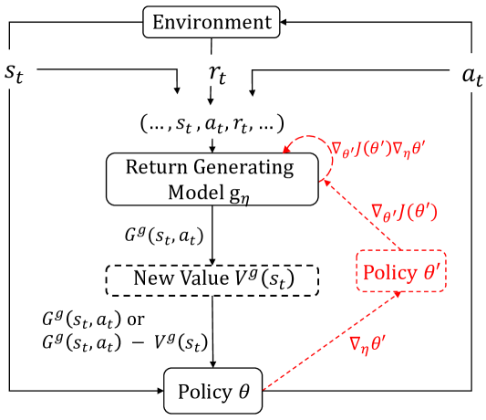
Figure 1: Relationship between Return Generating Model and existing policy gradient-based RL. We can optionally use a new value network to learn the new return generated by $g_{\eta}$, as shown by the dashed black box. The dashed red lines and box show how the return generating model $g_{\eta}$ can be trained using meta-learning and the chain rule.

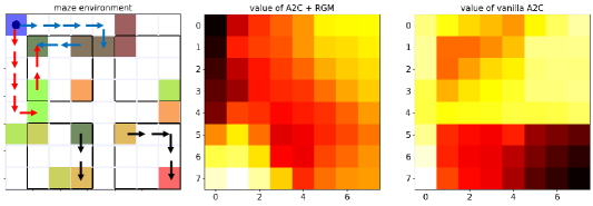
Figure 2: The values of grids of vanilla A2C (the value learns towards the traditional discounted sum return) and our A2C + RGM (the value learns towards to the return generated by RGM ). Darker color represents larger value. The value of A2C + RGM derives the correct path labeled by the red + black arrows in the leftmost panel, and the value of vanilla A2C derives another correct path labeled by blue + black arrows in the leftmost panel.

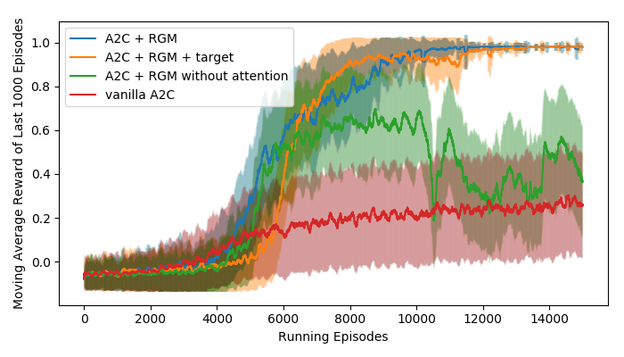
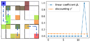
Figure 3: Left: Learning curves of the compared algorithms. The Y-axis is the moving average reward of the last 1000 episodes, and the shaded region is half a standard deviation. Middle and Right: Visualization of $\gamma^{t}$ and $\beta_{t}$ along the correct path, which is labeled by the arrows in the left maze.

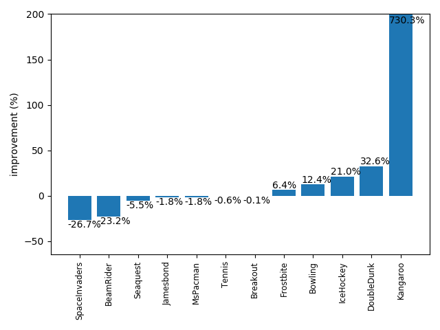
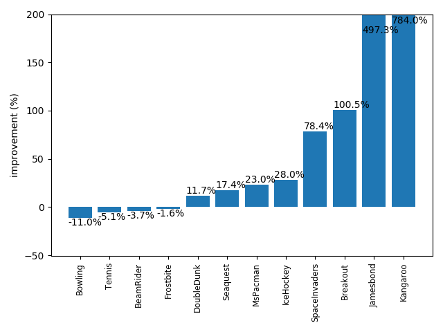
Figure 4: Left: Improvements of A2C + RGM over vanilla A2C. Right: Improvements of A2C + RGM over LIRPG. The y-axes show relative raw game score improvements.

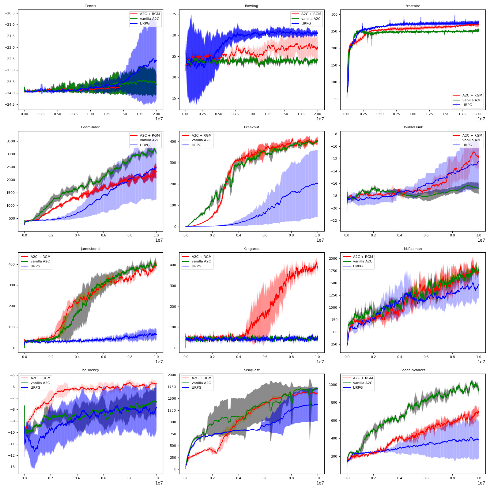
Figure 5: Comparison of Vanilla A2C and A2C + RGM on 12 Atari games. Red: A2C + RGM; Green: vanilla A2C. Blue: LIRPG. The X-axis is the trained time steps. The Y-axis is the raw game scores. The solid line is the mean of the raw scores in the last 100 episodes, averaged over 3 random seeds, and the shaded area is a standard deviation. As the large delayed-reward games Bowling, Tennis and Frostbite are very difficult to learn, we trained all algorithms on them for more time steps.

From New Return to New Value. The new return function naturally brings about a brand new value function. Indeed, we can similarly define the value of $V^{g}(s)$ and $Q^{g}(s,a)$ as the expected value of the new returns of trajectories starting from $s$ (taking action $a$), and following policy $\pi_{\theta}$:

$$\begin{split}G^{g}(\tau)&=G^{g}(s_{0},a_{0})=g_{\eta}(0,s_{0},a_{0},r_{0},...,s_{T},a_{T},r_{T},...)\\ V^{g}(s)=E_{\tau\sim\pi_{\theta}}[G^{g}(\tau)&|\tau(s_{0})=s],~{}~{}~{}~{}~{}~{}~{}~{}~{}~{}~{}Q^{g}(s,a)=E_{\tau\sim\pi_{\theta}}[G^{g}(\tau)|\tau(s_{0})=s,\tau(a_{0})=a]\\ \end{split}$$ (10)

Here we give a very shallow analysis on this new value definition (one obvious future work would be to give a deep analysis on such definitions). The new value definition is way more general than the original one, but this generality also loses useful properties, e.g., the Bellman Equation might no longer applies. In the classic RL setting, the bellman equation tells that the value of the current state can be computed by bootstrapping from the value of the next state $V(s_{t})=r_{t}+\gamma E_{s_{t+1}}[V(s_{t+1})]$, and the correction of such bootstrap might not hold true for an arbitrary return function $g$. As a result, temporal difference learning methods (e.g. Q-learning, SARSA) might not be applicable with the new value On the other hand, the Monte-Carlo methods for evaluating the new value would still work, which only relies on the Law of Big Number.

4 Experiments

4.1 General Setups

In this subsection, we describe some general setups for the following experiments. We implemented our RGM upon the A2C (Mnih et al., 2016) algorithm. All the experiment are running on a machine equipped with Intel(R) Xeon(R) CPU E5-2690, and four Nvidia Tesla M40 GPUs. In the following, we will denote the A2C baseline as the vanilla A2C, and denote our algorithms as A2C + RGM (short for Return Genearting Model). In both the illustrative case and the Atari experiment, the new form of return function is the linear combinations of the future rewards, as discussed in Section 3.2 and E.q. 4. The RGM $g_{\eta}$ has 4 stacking layers and 4 heads in multi-head attention.

4.2 Illustrative Case

In this section, we show our algorithm using an illustrative maze example. As shown in the leftmost panel of figure 2, the maze (MattChanTK, 2016) is a 2-D grid world of size $8\times 8$. The agent starts from the left-top corner, and needs to find its way to the exit at the bottom-right corner. Black lines in the maze represents unbreakable walls. The key feature of the maze is that it has portals, shown as colored grids in figure 2, which can transport the agent immediately from one location to another with the same color. Indeed, we deliberately created four isolated rooms in the maze, and to successfully reach the exit requires the agent to utilize these portals to transport between different rooms. Two possible routes have been marked out in figure 2.

At each time step, the agent gets a state which is the coordinate of his current location, chooses an moving direction among up, down, left and right, and receives a reward of $-\epsilon$ if he does not reach the exit, and $1$ if he reaches the exit, which also ends the game. We set $\epsilon$ to be very small, e.g., $-0.01$ in our experiments. Therefore, the maze renders an environment that has very delayed reward. Besides, from our human beings’ perspective, we would pay special attention to the portals, as they enable nonconsecutive spatial location change.

We compare the vanilla A2C algorithm and our A2C + RGM algorithm. We use separate value and policy networks, both of them are feed-forward MLPs with three hidden layers of 64 neurons and the ReLU nonlinear activation. Figure 3 (b) compares the learning curves of these two algorithms. For ablation study, we implemented two more versions of our A2C + RGM besides the vanilla one. 1) ‘RGM + target’: since our RGM is always learning (changing) itself, the learning objective it provides to the value network is also changing, which might cause oscillation for the learning of the value network. To alleviate this, similar to that in DQN (Mnih et al., 2013) and DDPG (Lillicrap et al., 2015), we use a target network of the RGM model and optimize the value network towards the target network to stabilize its learning. The parameters of the target network is copied from the learning RGM periodically. 2) ‘RGM without attention’: we replaced all the attention modules with feed-forward layers to test whether the attention module is necessary. The results in figure 3 (b) shows that our algorithm learns dramatically faster and better than the vanilla A2C algorithms. It also shows that the attention module is necessary for stable learning, and whether using a target network does not cause huge difference in learning in the maze environment.

To have a deeper understanding of how the RGM works, we visualized the values of the grids under the vanilla A2C’s value network and our A2C + RGM’s value network. The result is shown in figure 2. As expected, the values of grids learned in vanilla A2C exponentially decreases as the distance to the exit increases, and there is no difference in values between the transport grids and vanilla grids. However, the values learned by our RGM is quite different. It shows that a heavy part of return is redistributed to the beginning of the correct path that leads to the exit, and the value almost follows a decreasing trend as it approaches the exit. Also, compared with the vanilla values, the portals in our A2C + RGM tends to have higher values than the vanilla grids around it. Both values give the correct policy, as they all have higher values along the correct path. However, as indicated by Figure 3 (b), these two different values render large difference in the learning speed towards the optimal policy.

To further investigate how the new value is learned, we visualized the linear coefficient $\beta_{t}$ generated by our RGM along the correct path, and compared it with the traditional discounted $\gamma^{t}$. The result is shown in figure 3 (b). We normalize both coefficients to make them sum up to $1$. With $\gamma=0.99$, the discounted form return gives almost equal favour to each reward encountered along the path. On the contrast, our RGM distributed almost all the weight to the delayed reward at the last time step, which is the only positive reward the agent receives when reaching the exit. As a result, when using the traditional discounted return, the delayed reward (in our setting, which is also the only effective learning signal) is exponentially decayed $13$ times before it can reach the initial state, which greatly hurts its propagation; on the other hand, our RGM could propagate back this learning signal with nearly zero loss to all previous states (recall that our RGM compute return as $G^{g}(s_{t},a_{t})=\sum_{t=0}^{T}\beta_{t}r_{t}$, if some $\beta_{t}$ is near 1, then $r_{t}$ will be fully used when computing all $G(s_{i},a_{i}),~{}~{}i\leq t$). With this effective back propagation of the learning signal, our RGM greatly eases the learning of the agents.

4.3 Deep Reinforcement Learning Results on Atari Games

We also tested our A2C + RGM on multiple Atari games from the Arcade Learning Environment (ALE) Bellemare et al. (2013). We implemented the baseline A2C algorithm using Pytorch with exactly the same network architecture as in Mnih et al. (2016), and trained it using the same hyper-parameters as in the OpenAI implementation Dhariwal et al. (2017). We do not use a separate target network for the RGM as it does not bring significant help in the maze experiments.

We compare our A2C + RGM , with the vanilla A2C and LIRPG Zheng et al. (2018), in which the authors used the meta-learning methods to learn an intrinsic rewards at each time step instead of augmenting the return function. Figure 4 shows the improvements of A2C + RGM over the baseline methods, and Figure 5 shows the learning curves of all games. Among them, Bowling, Tennis, and Frosbite have very rare and delayed rewards, e.g., in Frostbite it takes the agent 180 time steps to get its first reward. DoubleDunk, IceHockey, Jamesbond and Kangaroo has an itermediate level of delayed rewards, e.g., the agent needs roughly 50 steps to get its first reward. The rest of the games, i.e., Seaquest, BeamRider, SpaceInvaders, Breakout and Mspacman all have rich immediate rewards. Using the original discounted sum return, learning in the delayed reward games are much more difficult than the rich-reward games. As shown in Figure 5, as expected, our A2C + RGM brings large benefits in the delayed games by learning a better form of return computation. For the non-delayed reward games, it boosts the performance in some of them, while hurts the performance in some others, as the original exponentially discounted return is already good enough for learning in such non-delayed games. For the RGM, there are two hyper-parameters: the learning rate $\alpha^{\prime}$ and the trajectory length $T$. We searched the following combinations of them $\{1e-4,1e-5,1e-6,1e-7\}\times\{50,100,200\}$, and plotted the best results from the search.

5 Conclusion

Return and value serve as the key objective that guide the learning of the policy. One key insight is that there could be many different ways to define the computation form of the return (and thus the value), from which the same optimal policy can be derived. However, these different forms could render dramatic difference in the learning speed. In this paper, we propose to use arbitrary general form for return computation, and designed an end-to-end algorithm to learn such general form to enhance policy learning by meta-gradient methods. We test our methods on a specially designed maze environment and several Atari games, and the experimental results show that our methods effectively learned new return computation forms that greatly improved learning performance.

References

- Arjona-Medina et al. (2018) Jose A Arjona-Medina, Michael Gillhofer, Michael Widrich, Thomas Unterthiner, and Sepp Hochreiter. Rudder: Return decomposition for delayed rewards. arXiv preprint arXiv:1806.07857, 2018.
- Babaeizadeh et al. (2017) Mohammad Babaeizadeh, Iuri Frosio, Stephen Tyree, Jason Clemons, and Jan Kautz. Reinforcement learning thorugh asynchronous advantage actor-critic on a gpu. In ICLR, 2017.
- Barnard (1993) Etienne Barnard. Temporal-difference methods and markov models. IEEE Transactions on Systems, Man, and Cybernetics, 23(2):357–365, 1993.
- Bellemare et al. (2013) M. G. Bellemare, Y. Naddaf, J. Veness, and M. Bowling. The arcade learning environment: An evaluation platform for general agents. Journal of Artificial Intelligence Research, 47:253–279, jun 2013.
- Bellemare et al. (2016) Marc Bellemare, Sriram Srinivasan, Georg Ostrovski, Tom Schaul, David Saxton, and Remi Munos. Unifying count-based exploration and intrinsic motivation. In Advances in Neural Information Processing Systems, pp. 1471–1479, 2016.
- Bellemare et al. (2013) Marc G Bellemare, Yavar Naddaf, Joel Veness, and Michael Bowling. The arcade learning environment: An evaluation platform for general agents. Journal of Artificial Intelligence Research, 47:253–279, 2013.
- Chentanez et al. (2005) Nuttapong Chentanez, Andrew G Barto, and Satinder P Singh. Intrinsically motivated reinforcement learning. In Advances in neural information processing systems, pp. 1281–1288, 2005.
- Dhariwal et al. (2017) Prafulla Dhariwal, Christopher Hesse, Oleg Klimov, Alex Nichol, Matthias Plappert, Alec Radford, John Schulman, Szymon Sidor, Yuhuai Wu, and Peter Zhokhov. Openai baselines. GitHub, GitHub repository, 2017.
- François-Lavet et al. (2015) Vincent François-Lavet, Raphael Fonteneau, and Damien Ernst. How to discount deep reinforcement learning: Towards new dynamic strategies. arXiv preprint arXiv:1512.02011, 2015.
- Icarte et al. (2018) Rodrigo Toro Icarte, Toryn Klassen, Richard Valenzano, and Sheila McIlraith. Using reward machines for high-level task specification and decomposition in reinforcement learning. In International Conference on Machine Learning, pp. 2112–2121, 2018.
- Jaderberg et al. (2016) Max Jaderberg, Volodymyr Mnih, Wojciech Marian Czarnecki, Tom Schaul, Joel Z Leibo, David Silver, and Koray Kavukcuoglu. Reinforcement learning with unsupervised auxiliary tasks. arXiv preprint arXiv:1611.05397, 2016.
- Kingma & Ba (2014) Diederik P Kingma and Jimmy Ba. Adam: A method for stochastic optimization. arXiv preprint arXiv:1412.6980, 2014.
- Lattimore & Hutter (2011) Tor Lattimore and Marcus Hutter. Time consistent discounting. In International Conference on Algorithmic Learning Theory, pp. 383–397. Springer, 2011.
- Lillicrap et al. (2015) Timothy P Lillicrap, Jonathan J Hunt, Alexander Pritzel, Nicolas Heess, Tom Erez, Yuval Tassa, David Silver, and Daan Wierstra. Continuous control with deep reinforcement learning. arXiv preprint arXiv:1509.02971, 2015.
- Machado et al. (2017) Marlos C. Machado, Marc G. Bellemare, Erik Talvitie, Joel Veness, Matthew J. Hausknecht, and Michael Bowling. Revisiting the arcade learning environment: Evaluation protocols and open problems for general agents. CoRR, abs/1709.06009, 2017.
- Martin et al. (2017) Jarryd Martin, Suraj Narayanan Sasikumar, Tom Everitt, and Marcus Hutter. Count-based exploration in feature space for reinforcement learning. In Proceedings of the International Joint Conference on Artificial Intelligence (IJCAI), 2017.
- MattChanTK (2016) MattChanTK. Mattchantk/gym-maze, 2016. URL https://github.com/MattChanTK/gym-maze.
- Mirowski et al. (2016) Piotr Mirowski, Razvan Pascanu, Fabio Viola, Hubert Soyer, Andrew J Ballard, Andrea Banino, Misha Denil, Ross Goroshin, Laurent Sifre, Koray Kavukcuoglu, et al. Learning to navigate in complex environments. arXiv preprint arXiv:1611.03673, 2016.
- Mnih et al. (2013) Volodymyr Mnih, Koray Kavukcuoglu, David Silver, Alex Graves, Ioannis Antonoglou, Daan Wierstra, and Martin Riedmiller. Playing atari with deep reinforcement learning. arXiv preprint arXiv:1312.5602, 2013.
- Mnih et al. (2016) Volodymyr Mnih, Adria Puigdomenech Badia, Mehdi Mirza, Alex Graves, Timothy Lillicrap, Tim Harley, David Silver, and Koray Kavukcuoglu. Asynchronous methods for deep reinforcement learning. In International Conference on Machine Learning, pp. 1928–1937, 2016.
- Ng et al. (1999) Andrew Y Ng, Daishi Harada, and Stuart Russell. Policy invariance under reward transformations: Theory and application to reward shaping. In ICML, volume 99, pp. 278–287, 1999.
- Oh et al. (2020) Junhyuk Oh, Matteo Hessel, Wojciech M Czarnecki, Zhongwen Xu, Hado van Hasselt, Satinder Singh, and David Silver. Discovering reinforcement learning algorithms. arXiv preprint arXiv:2007.08794, 2020.
- OpenAI (2018) OpenAI. Openai five. https://blog.openai.com/openai-five/, 2018.
- Oudeyer & Kaplan (2009) Pierre-Yves Oudeyer and Frederic Kaplan. What is intrinsic motivation? a typology of computational approaches. Frontiers in neurorobotics, 1:6, 2009.
- Pitis (2019) Silviu Pitis. Rethinking the discount factor in reinforcement learning: A decision theoretic approach. arXiv preprint arXiv:1902.02893, 2019.
- Reinke et al. (2017) Chris Reinke, Eiji Uchibe, and Kenji Doya. Average reward optimization with multiple discounting reinforcement learners. In International Conference on Neural Information Processing, pp. 789–800. Springer, 2017.
- Romoff et al. (2019) Joshua Romoff, Peter Henderson, Ahmed Touati, Yann Ollivier, Emma Brunskill, and Joelle Pineau. Separating value functions across time-scales. arXiv preprint arXiv:1902.01883, 2019.
- Schmidhuber (2010) Jürgen Schmidhuber. Formal theory of creativity, fun, and intrinsic motivation (1990–2010). IEEE Transactions on Autonomous Mental Development, 2(3):230–247, 2010.
- Schulman et al. (2017) John Schulman, Filip Wolski, Prafulla Dhariwal, Alec Radford, and Oleg Klimov. Proximal policy optimization algorithms. arXiv preprint arXiv:1707.06347, 2017.
- Sherstan et al. (2018) Craig Sherstan, James MacGlashan, and Patrick M Pilarski. Generalizing value estimation over timescale. Network, 2:3, 2018.
- Singh (1992) Satinder P Singh. Scaling reinforcement learning algorithms by learning variable temporal resolution models. In Machine Learning Proceedings 1992, pp. 406–415. Elsevier, 1992.
- Stadie et al. (2016) Bradly C Stadie, Sergey Levine, and Pieter Abbeel. Incentivizing exploration in reinforcement learning with deep predictive models. In ICLR, 2016.
- Sutton et al. (1998) Richard S Sutton, Andrew G Barto, et al. Introduction to reinforcement learning, volume 135. MIT press Cambridge, 1998.
- Sutton et al. (2000) Richard S Sutton, David A McAllester, Satinder P Singh, and Yishay Mansour. Policy gradient methods for reinforcement learning with function approximation. In Advances in neural information processing systems, pp. 1057–1063, 2000.
- Sutton et al. (2011) Richard S Sutton, Joseph Modayil, Michael Delp, Thomas Degris, Patrick M Pilarski, Adam White, and Doina Precup. Horde: A scalable real-time architecture for learning knowledge from unsupervised sensorimotor interaction. In The 10th International Conference on Autonomous Agents and Multiagent Systems-Volume 2, pp. 761–768. International Foundation for Autonomous Agents and Multiagent Systems, 2011.
- Tang et al. (2017) Haoran Tang, Rein Houthooft, Davis Foote, Adam Stooke, OpenAI Xi Chen, Yan Duan, John Schulman, Filip DeTurck, and Pieter Abbeel. # exploration: A study of count-based exploration for deep reinforcement learning. In Advances in Neural Information Processing Systems, pp. 2750–2759, 2017.
- Tieleman & Hinton (2012) Tijmen Tieleman and Geoffrey Hinton. Lecture 6.5-rmsprop: Divide the gradient by a running average of its recent magnitude. COURSERA: Neural networks for machine learning, 4(2):26–31, 2012.
- Vaswani et al. (2017) Ashish Vaswani, Noam Shazeer, Niki Parmar, Jakob Uszkoreit, Llion Jones, Aidan N Gomez, Łukasz Kaiser, and Illia Polosukhin. Attention is all you need. In Advances in neural information processing systems, pp. 5998–6008, 2017.
- Veeriah et al. (2019) Vivek Veeriah, Matteo Hessel, Zhongwen Xu, Janarthanan Rajendran, Richard L Lewis, Junhyuk Oh, Hado P van Hasselt, David Silver, and Satinder Singh. Discovery of useful questions as auxiliary tasks. In Advances in Neural Information Processing Systems, pp. 9310–9321, 2019.
- Xu et al. (2018) Zhongwen Xu, Hado P van Hasselt, and David Silver. Meta-gradient reinforcement learning. In Advances in Neural Information Processing Systems, pp. 2396–2407, 2018.
- Xu et al. (2020) Zhongwen Xu, Hado van Hasselt, Matteo Hessel, Junhyuk Oh, Satinder Singh, and David Silver. Meta-gradient reinforcement learning with an objective discovered online. arXiv preprint arXiv:2007.08433, 2020.
- Zahavy et al. (2020) Tom Zahavy, Zhongwen Xu, Vivek Veeriah, Matteo Hessel, Junhyuk Oh, Hado van Hasselt, David Silver, and Satinder Singh. Self-tuning deep reinforcement learning. arXiv preprint arXiv:2002.12928, 2020.
- Zheng et al. (2018) Zeyu Zheng, Junhyuk Oh, and Satinder Singh. On learning intrinsic rewards for policy gradient methods. In Advances in Neural Information Processing Systems, pp. 4644–4654, 2018.