Estimating and Inferring the Maximum Degree of Stimulus-Locked Time-Varying Brain Connectivity Networks

Abstract

Neuroscientists have enjoyed much success in understanding brain functions by constructing brain connectivity networks using data collected under highly controlled experimental settings. However, these experimental settings bear little resemblance to our real-life experience in day-to-day interactions with the surroundings. To address this issue, neuroscientists have been measuring brain activity under natural viewing experiments in which the subjects are given continuous stimuli, such as watching a movie or listening to a story. The main challenge with this approach is that the measured signal consists of both the stimulus-induced signal, as well as intrinsic-neural and non-neuronal signals. By exploiting the experimental design, we propose to estimate stimulus-locked brain network by treating non-stimulus-induced signals as nuisance parameters. In many neuroscience applications, it is often important to identify brain regions that are connected to many other brain regions during cognitive process. We propose an inferential method to test whether the maximum degree of the estimated network is larger than a pre-specific number. We prove that the type I error can be controlled and that the power increases to one asymptotically. Simulation studies are conducted to assess the performance of our method. Finally, we analyze a functional magnetic resonance imaging dataset obtained under the Sherlock Holmes movie stimuli.

Keywords: Gaussian multiplier bootstrap; Hypothesis testing; Inter-subject; Latent variables; Maximum degree; Subject specific effects.

1 Introduction

In the past few decades, much effort has been put into understanding task-based brain connectivity networks. For instance, in a typical visual mapping experiment, subjects are presented with a simple static visual stimulus and are asked to maintain fixation at the visual stimulus, while their brain activities are measured. Under such highly controlled experimental settings, numerous studies have shown that there are substantial similarities across brain connectivity networks constructed for different subjects (Press et al. 2001, Hasson et al. 2003). However, such experimental settings bear little resemblance to our real-life experience in several aspects: natural viewing consists of a continuous stream of perceptual stimuli; subjects can freely move their eyes; there are interactions among viewing, context, and emotion (Hasson et al. 2004). To address this issue, neuroscientists have started measuring brain activity under continuous natural stimuli, such as watching a movie or listening to a story (Hasson et al. 2004, Simony et al. 2016, Chen et al. 2017). The main scientific question is to understand the dynamics of the brain connectivity network that are specific to the continuous natural stimuli.

In the neuroscience literature, a typical approach for constructing a brain connectivity network is to calculate a sample covariance matrix for each subject: the covariance matrix encodes marginal relationships for each pair of brain regions within each subject. More recently, graphical models have been used in modeling brain connectivity networks: graphical models encode conditional dependence relationships between each pair of brain regions, given the others (Rubinov & Sporns 2010). A graph consists of $d$ nodes, each representing a random variable, as well as a set of edges joining pairs of nodes corresponding to conditionally dependent variables. There is a vast literature on learning the structure of static undirected graphical models, and we refer the reader to Drton & Maathuis (2017) for a detailed review.

Under natural continuous stimuli, it is often of interest to estimate a dynamic brain connectivity network, i.e., a graph that changes over time. A natural candidate for this purpose is the time-varying Gaussian graphical model (Zhou et al. 2010, Kolar et al. 2010). The time-varying Gaussian graphical model assumes

$$\bm{X}(z)\mid Z=z\sim N_{d}\{\mathbf{0},\bm{\Sigma}_{X}(z)\},$$ (1)

where $\bm{\Sigma}_{X}(z)$ is the covariance matrix of $\bm{X}(z)$ given $Z=z$, and $Z\in[0,1]$ has a continuous density. The inverse covariance matrix $\{\bm{\Sigma}_{X}(z)\}^{-1}$ encodes conditional dependence relationships between pairs of random variables at time $Z=z$: $\{\bm{\Sigma}_{X}(z)\}^{-1}_{jk}=0$ if and only if the $j$th and $k$th variables are conditionally independent given the other variables at time $Z=z$.

In natural viewing experiments, the main goal is to construct a brain connectivity network that is locked to the processing of external stimuli, referred to as stimulus-locked network (Simony et al. 2016, Chen et al. 2017, Regev et al. 2018). Constructing a stimulus-locked network can better characterize the dynamic changes of brain patterns across the continuous stimulus (Simony et al. 2016). The main challenge in constructing stimulus-locked network is the lack of highly controlled experiments that remove spontaneous and individual variations. The measured blood-oxygen-level dependent (BOLD) signal consists of not only signal that is specific to the stimulus, but also intrinsic neural signal (random fluctuations) and non-neuronal signal (physiological noise) that are specific to each subject. The intrinsic neural signal and non-neuronal signal can be interpreted as measurement error or latent variables that confound the stimuli-specific signal. We refer to non-stimulus-induced signals as subject specific effects throughout the manuscript. Thus, directly fitting (1) using the measured data will yield a time-varying graph that primarily reflects intrinsic BOLD fluctuations within each brain rather than BOLD fluctuations due to the natural continuous stimulus.

In this paper, we exploit the experimental design aspect of natural viewing experiments and propose to estimate a dynamic stimulus-locked brain connectivity network by treating the intrinsic neural signal and non-neuronal signal as nuisance parameters. Our proposal exploits the fact that the same stimulus will be given to multiple independent subjects, and that the intrinsic neural signal and non-neuronal signal for different subjects are independent. Thus, this motivates us to estimate a brain connectivity network across two brains rather than within each brain. In fact, this approach has been considered in Simony et al. (2016) and Chen et al. (2017) where they estimated brain connectivity networks by calculating covariance for brain regions between two brains.

After estimating the stimulus-locked brain connectivity network, the next important question is to infer whether there are any regions of interest that are connected to many other regions of interest during cognitive process (Hagmann et al. 2008). These highly connected brain regions are referred to as hub nodes, and the number of connections for each brain region is referred to as degree. Identifying hub brain regions that are specific to the given natural continuous stimulus will lead to a better understanding of the cognitive processes in the brain, and may shed light on various cognitive disorders. In the existing literature, several authors have proposed statistical methodologies to estimate networks with hubs (see, for instance, Tan et al. 2014). In this paper, we instead focus on developing a novel inferential framework to test the hypothesis whether there exists at least one time point such that the maximum degree of the graph is greater than $k$.

Our proposed inferential framework is motivated by two major components: (1) the Gaussian multiplier bootstrap for approximating the distribution of supreme of empirical processes (Chernozhukov et al. 2013, 2014b), and (2) the step-down method for multiple hypothesis testing problems (Romano & Wolf 2005). In a concurrent work, Neykov et al. (2019) proposed a framework for testing general graph structure on a static graph. In Appendix A, we will show that our proposed method can be extended to testing a large family of graph structures similar to that of Neykov et al. (2019).

2 Stimulus-Locked Time-Varying Brain Connectivity Networks

2.1 A Statistical Model

Let $\bm{X}(z)$, $\bm{S}(z)$, $\bm{E}(z)$ be the observed data, stimulus-induced signal, and subject specific effects at time $Z=z$, respectively. Assume that $Z$ is a continuous random variable with a continuous density. For a given $Z=z$, we model the observed data as the summation of stimulus-induced signal and the subject specific effects:

$$\bm{X}(z)=\bm{S}(z)+\bm{E}(z),\quad\bm{S}(z)\mid Z=z\sim N_{d}\{\mathbf{0},\bm{\Sigma}(z)\},\quad\bm{E}(z)\mid Z=z\sim N_{d}\{\mathbf{0},\mathbf{L}_{X}(z)\},$$ (2)

where $\bm{\Sigma}(z)$ is the covariance matrix of the stimulus-induced signal, and $\mathbf{L}_{X}(z)$ is the covariance matrix of the subject specific effects. We assume that $\bm{S}(z)$ and $\bm{E}(z)$ are independent for all $z$. Thus, estimating the stimulus-locked brain connectivity network amounts to estimating $\{\bm{\Sigma}(z)\}^{-1}$. Fitting the model in (1) using the observed data will yield an estimate of $\{\bm{\Sigma}(z)+\mathbf{L}_{X}(z)\}^{-1}$, and thus, (1) fails to estimate the stimulus-locked brain connectivity network $\{\bm{\Sigma}(z)\}^{-1}$.

To address this issue, we exploit the experimental design aspect of natural viewing experiments. In many studies, neuroscientists often measure brain activity for multiple subjects under the same continuous natural stimulus (Chen et al. 2017, Simony et al. 2016). Let $\bm{X}(z)$ and $\bm{Y}(z)$ be measured data for two subjects at time point $Z=z$. Since the same natural stimulus is given to both subjects, this motivates the following statistical model:

$$\begin{split}\bm{X}(z)=\bm{S}(z)+\bm{E}_{X}(z),\qquad\bm{Y}(z)=\bm{S}(z)+&\bm{E}_{Y}(z),\qquad\bm{S}(z)|Z=z\sim N_{d}\{\mathbf{0},\bm{\Sigma}(z)\},\\ \bm{E}_{X}(z)|Z=z\sim N_{d}\{\mathbf{0},\mathbf{L}_{X}(z)\},&~{}~{}~{}~{}\bm{E}_{Y}(z)|Z=z\sim N_{d}\{\mathbf{0},\mathbf{L}_{Y}(z)\},\end{split}$$ (3)

where $\bm{S}(z)$ is the stimulus-induced signal, and $\bm{E}_{X}(z)$ and $\bm{E}_{Y}(z)$ are the subject specific effects at $Z=z$. Model (3) motivates the calculation of inter-subject covariance between two subjects rather than the within-subject covariance. For a given time point $Z=z$, we have

$$\mathbb{E}[\bm{X}(z)\{\bm{Y}(z)\}^{T}\mid Z=z]=\mathbb{E}[\bm{S}(z)\{\bm{S}(z)\}^{T}\mid Z=z]+\mathbb{E}[\bm{E}_{X}(z)\{\bm{E}_{Y}(z)\}^{T}\mid Z=z]=\bm{\Sigma}(z).$$

That is, we estimate $\bm{\Sigma}(z)$ via the inter-subject covariance by treating $\mathbf{L}_{X}(z)$ and $\mathbf{L}_{Y}(z)$ as nuisance parameters. In the neuroscience literature, several authors have been calculating inter-subject covariance matrix to estimate marginal dependencies among brain regions that are stimulus-locked (Chen et al. 2017, Simony et al. 2016). They have found that calculating the inter-subject covariance is able to better capture the stimulus-locked marginal relationships for pairs of brain regions.

For simplicity, throughout the paper, we focus on two subjects. When there are multiple subjects, we can split the subjects into two groups, and obtain an average of each group to estimate the stimulus-locked brain network. We also discuss a $U$-statistic type estimator for the case when there are multiple subjects in Appendix B.

2.2 Inter-Subject Time-Varying Gaussian Graphical Models

We now propose inter-subject time-varying Gaussian graphical models for estimating stimulus-locked time-varying brain networks. Let $(Z_{1},\bm{X}_{1},\bm{Y}_{1}),\ldots,(Z_{n},\bm{X}_{n},\bm{Y}_{n})$ be $n$ independent realizations of the triplets $(Z,\bm{X},\bm{Y})$. Both subjects share the same $Z_{1},\ldots,Z_{n}$ since they are given the same continuous stimulus. Let $K:\mathbb{R}\rightarrow\mathbb{R}$ be a symmetric kernel function. To obtain an estimate for $\bm{\Sigma}(z)$, we propose the inter-subject kernel smoothed covariance estimator

$$\widehat{\bm{\Sigma}}(z)=\frac{\sum_{i\in[n]}K_{h}(Z_{i}-z)\bm{X}_{i}\bm{Y}_{i}^{T}}{\sum_{i\in[n]}K_{h}(Z_{i}-z)},$$ (4)

where $K_{h}(Z_{i}-z)=K\{(Z_{i}-z)/h\}/h$, $h>0$ is the bandwidth parameter, and $[n]=\{1,\ldots,n\}$. For simplicity, we use the Epanechnikov kernel

$$K(u)=0.75\cdot\left(1-u^{2}\right)\cdot\operatorname{\mathds{1}}_{\{|u|\leq 1\}},$$ (5)

where $\operatorname{\mathds{1}}_{\{|u|\leq 1\}}$ is an indicator function that takes value one if $|u|\leq 1$ and zero otherwise. The choice of kernel is not essential as long as it satisfies regularity conditions in Section 5.1.

Let $\bm{\Theta}(z)=\{\bm{\Sigma}(z)\}^{-1}$. Given the kernel smoothed inter-subject covariance estimator in (27), there are multiple approaches to obtain an estimate of the inverse covariance matrix $\bm{\Theta}(z)$. We consider the CLIME estimator proposed by Cai et al. (2011). Let $\mathbf{e}_{j}$ be the $j$th canonical basis in $\mathbb{R}^{d}$. For a vector $\mathbf{v}\in\mathbb{R}^{d}$, let $\|\mathbf{v}\|_{1}=\sum_{j=1}^{d}|v_{j}|$ and let $\|\mathbf{v}\|_{\infty}=\max_{j}|v_{j}|$. For each $j\in[d]$, the CLIME estimator takes the form

$$\widehat{\bm{\Theta}}_{j}(z)=\underset{\bm{\theta}\in\mathbb{R}^{d}}{\mathop{\mathrm{argmin}}}\;\|\bm{\theta}\|_{1}\qquad\mathrm{subject\;to\;}\left\|\widehat{\bm{\Sigma}}(z)\cdot\bm{\theta}-\mathbf{e}_{j}\right\|_{\infty}\leq\lambda,$$ (6)

where $\lambda>0$ is a tuning parameter that controls the sparsity of $\widehat{\bm{\Theta}}_{j}(z)$. We construct an estimator for the stimulus-locked brain network as $\widehat{\bm{\Theta}}(z)=[\{\widehat{\bm{\Theta}}_{1}(z)\}^{T},\ldots,\{\widehat{\bm{\Theta}}_{d}(z)\}^{T}]$.

There are two tuning parameters in our proposed method: a bandwidth parameter $h$ that controls the smoothness of the estimated covariance matrix, and a tuning parameter $\lambda$ that controls the sparsity of the estimated network. The bandwidth parameter $h$ can be selected according to the scientific context. For instance, in many neuroscience applications that involve continuous natural stimuli, we select $h$ such that there are always at least 30% of the time points that have non-zero kernel weights. In the following, we propose a $L$-fold cross-validation type procedure to select $\lambda$. We first partition the $n$ time points into $L$ folds. Let $C_{\ell}$ be an index set containing time points for the $\ell$th fold. Let $\bm{\Theta}(z)^{(-\ell)}$ be the estimated inverse covariance matrix using data excluding the $\ell$th fold, and let $\bm{\Sigma}(z)^{(\ell)}$ be the estimated kernel smoothed covariance estimated using data only from the $\ell$th fold. We calculate the following quantity for various values of $\lambda$ :

$$\mathrm{cv}_{\lambda}=\frac{1}{L}\sum_{\ell=1}^{L}\sum_{i\in C_{\ell}}\|\widehat{\bm{\Sigma}}(z_{i},\lambda)^{(\ell)}\widehat{\bm{\Theta}}{(z_{i},\lambda)}^{(-\ell)}-\mathbf{I}_{d}\|_{\max},$$ (7)

where $\|\cdot\|_{\max}$ is the element-wise max norm for matrix. From performing extensive numerical studies, we find that picking $\lambda$ that minimizes the above quantity tend to be too conservative. We instead propose to pick the smallest $\lambda$ with $\mathrm{cv}_{\lambda}$ smaller than the minimum plus two standard deviation.

2.3 Inference on Maximum Degree

We consider testing the hypothesis:

$$\small\begin{split}&H_{0}:\mathrm{\;for\;all\;}z\in[0,1],\mathrm{\;the\;maximum\;degree\;of\;the\;graph\;is\;not\;greater\;than\;}k,\\ &H_{1}:\mathrm{\;there\;exists\;a\;}z_{0}\in[0,1]\mathrm{\;such\;that\;the\;maximum\;degree\;of\;the\;graph\;is\;greater\;than\;}k.\\ \end{split}$$ (8)

In the existing literature, many authors have proposed to test whether there is an edge between two nodes in a graph (see, Neykov et al. 2018, and the references therein). Due to the $\ell_{1}$ penalty used to encourage a sparse graph, classical test statistics are no longer asymptotically normal. We employ the de-biased test statistic

$$\widehat{\bm{\Theta}}^{\mathrm{de}}_{jk}(z)=\widehat{\bm{\Theta}}_{jk}(z)-\frac{\left\{\widehat{\bm{\Theta}}_{j}(z)\right\}^{T}\left\{\widehat{\bm{\Sigma}}(z)\widehat{\bm{\Theta}}_{k}(z)-\mathbf{e}_{k}\right\}}{\left\{\widehat{\bm{\Theta}}_{j}(z)\right\}^{T}\widehat{\bm{\Sigma}}_{j}(z)},$$ (9)

where $\widehat{\bm{\Theta}}_{j}(z)$ is the $j$th column of $\widehat{\bm{\Theta}}(z)$. The subtrahend in (9) is the bias introduced by imposing an $\ell_{1}$ penalty during the estimation procedure.

We use (9) to construct a test statistic for testing the maximum degree of a time-varying graph. Let $G(z)=\{V,E(z)\}$ be an undirected graph, where $V=\{1,\ldots,d\}$ is a set of $d$ nodes and $E(z)\subseteq V\times V$ is a set of edges connecting pairs of nodes. Let

$$T_{E}=\underset{z\in[0,1]}{\sup}\;\underset{(j,k)\in E(z)}{\max}\;\sqrt{nh}\cdot\left|\widehat{\bm{\Theta}}^{\mathrm{de}}_{jk}(z)-\bm{\Theta}_{jk}(z)\right|\cdot\left\{\frac{1}{n}\sum_{i\in[n]}K_{h}(Z_{i}-z)\right\}.$$ (10)

The edge set $E(z)$ is defined based on the hypothesis testing problem. In the context of testing maximum degree of a time-varying graph as in (8), $E(z)=V\times V$, and therefore the maximum is taken over all possible edges between pairs of nodes. Throughout the manuscript, we will use the notation $E(z)$ to indicate some predefined known edge set. This general edge set will be different for testing different graph structures, and we refer the reader to Appendix A for details.

Since the test statistic (10) involves taking the supreme over $z$ and the maximum over all edges in $E(z)$, it is challenging to evaluate its asymptotic distribution. To this end, we generalize the Gaussian multiplier bootstrap proposed in Chernozhukov et al. (2013) and Chernozhukov et al. (2014b) to approximate the distribution of the test statistic $T_{E}$. Let $\xi_{1},\ldots,\xi_{n}\stackrel{{\scriptstyle\mathrm{i.i.d.}}}{{\sim}}N(0,1)$. We construct the bootstrap statistic as

$$T^{B}_{E}=\underset{z\in[0,1]}{\sup}\;\underset{(j,k)\in E(z)}{\max}\;\sqrt{nh}\cdot\left|\frac{\sum_{i\in[n]}\left\{\widehat{\bm{\Theta}}_{j}(z)\right\}^{T}K_{h}(Z_{i}-z)\left\{\bm{X}_{i}\bm{Y}_{i}^{T}\widehat{\bm{\Theta}}_{k}(z)-\mathbf{e}_{k}\right\}\xi_{i}/n}{\left\{\widehat{\bm{\Theta}}_{j}(z)\right\}^{T}\widehat{\bm{\Sigma}}_{j}(z)}\right|.$$ (11)

We denote the conditional $(1-\alpha)$-quantile of $T^{B}_{E}$ given $\{(Z_{i},\bm{X}_{i},\bm{Y}_{i})\}_{i\in[n]}$ as

$$c(1-\alpha,E)=\inf\left(t\in\mathbb{R}\;|\;P\left[T^{B}_{E}\leq t\;|\;\{(Z_{i},\bm{X}_{i},\bm{Y}_{i})\}_{i\in[n]}\right]\geq 1-\alpha\right).$$ (12)

The quantity $c(1-\alpha,E)$ can be calculated numerically using Monte-Carlo. In Section 5.2, we show that the quantile of $T_{E}$ in (10) can be estimated accurately by the conditional $(1-\alpha)$-quantile of the bootstrap statistic.

We now propose an inference framework for testing hypothesis problem of the form (8). Our proposed method is motivated by the step-down method in Romano & Wolf (2005) for multiple hypothesis tests. The details are summarized in Algorithm 1. Algorithm 1 involves evaluating all values of $z\in[0,1]$. In practice, we implement the proposed method by discretizing values of $z\in[0,1]$ into a large number of time points. We note that there will be approximation error by taking the maximum over the discretized time points instead of the supremum of the continuous trajectory. The approximation error could be reduced to arbitrarily small if we increase the density of discretization.

Algorithm 1 Testing Maximum Degree of a Time-Varying Graph.

Input: type I error $\alpha$; pre-specified degree $k$; de-biased estimator $\widehat{\bm{\Theta}}^{\mathrm{de}}(z)$ for $z\in[0,1]$.

1. Compute the conditional quantile

   $$c(1-\alpha,E)=\inf\left[t\in\mathbb{R}\mid P(T^{B}_{E})\leq t\mid\{(Z_{i},\bm{X}_{i},\bm{Y}_{i})\}_{i\in[n]}\geq 1-\alpha\right],$$

   where $T^{B}_{E}$ is the bootstrap statistic defined in (11).

2. Construct the rejected edge set

   $$\mathcal{R}(z)=\left\{e\in E(z)\mid\sqrt{nh}\cdot|\widehat{\bm{\Theta}}_{e}^{d}(z)|\cdot\sum_{i\in[n]}K_{h}(Z_{i}-z)/n>c(1-\alpha,E)\right\}.$$

3. Compute $d_{\mathrm{rej}}$ as the maximum degree of the dynamic graph based on the rejected edge set.

Output: Reject the null hypothesis if $d_{\mathrm{rej}}>k$.

In Section 5.2, we will show that Algorithm 1 is able to control the type I error at a pre-specified value $\alpha$. Moreover, the power of the proposed inferential method increases to one as we increase the number of time points $n$. In fact, the proposed inferential method can be generalized to testing a wide variety of structures that satisfy the monotone graph property. Some examples of monotone graph property are that the graph is connected, the graph has no more than $k$ connected components, the maximum degree of the graph is larger than $k$, the graph has no more than $k$ isolated nodes, and the graph contains a clique of size larger than $k$. This generalization will be presented in Appendix A.

3 Simulation Studies

We perform numerical studies to evaluate the performance of our proposal using the inter-subject covariance relative to the typical time-varying Gaussian graphical model using within-subject covariance. To this end, we define the true positive rate as the proportion of correctly identified non-zeros in the true inverse covariance matrix, and the false positive rate as the proportion of zeros that are incorrectly identified to be non-zeros. To evaluate our testing procedure, we calculate the type I error rate and power as the proportion of falsely rejected $H_{0}$ and correctly rejected $H_{0}$, respectively, over a large number of data sets.

To generate the data, we first construct the inverse covariance matrix $\bm{\Theta}(z)$ for $z=\{0,0.2,0.5\}$. At $z=0$, we set $(d-2)/4$ off-diagonal elements of $\bm{\Theta}(0)$ to equal 0.3 randomly with equal probability. At $z=0.2$, we set an additional $(d-2)/4$ off-diagonal elements of $\bm{\Theta}(0)$ to equal 0.3. At $z=0.5$, we randomly select two columns of $\bm{\Theta}(0.2)$ and add $k+1$ edges to each of the two columns. This guarantees that the maximum degree of the graph is greater than $k$. To ensure that the inverse covariance matrix is smooth, for $z\in[0,0.2]$, we construct $\bm{\Theta}(z)$ by taking linear interpolations between the elements of $\bm{\Theta}(0)$ and $\bm{\Theta}(0.2)$. For $z\in[0.2,0.5]$, we construct $\bm{\Theta}(z)$ in a similar fashion based on $\bm{\Theta}(0.2)$ and $\bm{\Theta}(0.5)$. The construction is illustrated in Figure 1.

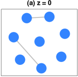
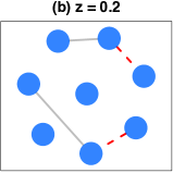
Figure 1: (a): A graph corresponding to $\bm{\Theta}(0)$ with maximum degree no greater than four. (b): A graph corresponding to $\bm{\Theta}(0.2)$ with maximum degree less than or equal to four. The red dash edges are additional edges that are added to $\bm{\Theta}(0)$. (c): A graph corresponding to $\bm{\Theta}(0.5)$ with maximum degree larger than four. The red dash edges are additional edges that are added to $\bm{\Theta}(0.2)$ such that the maximum degree of the graph is larger than four.

To ensure that the inverse covariance matrix is positive definite, we set $\bm{\Theta}_{jj}(z)=|\Lambda_{\min}\{\bm{\Theta}(z)\}|+0.1$, where $\Lambda_{\min}\{\bm{\Theta}(z)\}$ is the minimum eigenvalue of $\bm{\Theta}(z)$. We then rescale the matrix such that the diagonal elements of $\bm{\Theta}(z)$ equal one. The covariance $\bm{\Sigma}(z)$ can be obtained by taking the inverse of $\bm{\Theta}(z)$ for each value of $z$. Model (3) involves the subject specific covariance matrix $\mathbf{L}_{X}(z)$ and $\mathbf{L}_{Y}(z)$. For simplicity, we assume that these covariance matrices stay constant over time. We generate $\mathbf{L}_{X}$ by setting the diagonal elements to be one and the off-diagonal elements to be 0.3. Then, we add random perturbations $\epsilon_{k}\epsilon_{k}^{T}$ to $\mathbf{L}_{X}$ for $k=1,\ldots,10$, where $\epsilon_{k}\sim N_{d}(\mathbf{0},\mathbf{I}_{d})$. The matrix $\mathbf{L}_{Y}$ is generated similarly.

To generate the data according to (3), we first generate $Z_{i}\sim\mathrm{Unif}(0,1)$. Given $Z_{1},\ldots,Z_{n}$, we generate $\bm{S}(Z_{i})\mid Z=Z_{i}\sim N_{d}\{\mathbf{0},\bm{\Sigma}(Z_{i})\}$. We then simulate $\bm{E}_{X}(Z_{i})\mid Z=Z_{i}\sim N_{d}(\mathbf{0},\mathbf{L}_{X})$ and $\bm{E}_{Y}(Z_{i})\mid Z=Z_{i}\sim N_{d}(\mathbf{0},\mathbf{L}_{Y})$. Finally, for each value of $Z$, we generate

$$\bm{X}(Z_{i})=\bm{S}(Z_{i})+\bm{E}_{X}(Z_{i})\qquad\mathrm{and}\qquad\bm{Y}(Z_{i})=\bm{S}(Z_{i})+\bm{E}_{Y}(Z_{i}).$$

Note that both $\bm{X}(Z_{i})$ and $\bm{Y}(Z_{i})$ share the same generated $\bm{S}(Z_{i})$ since both subjects will be given the same natural continuous stimulus. In the following sections, we will assess the performance of our proposal relative to that of typical approach for time-varying Gaussian graphical models using the. within-subject covariance matrix as input. We then evaluate the proposed inferential procedure in Section 2.3 by calculating its type I error and power.

3.1 Estimation

To mimic the data application we consider, we generate the data with $n=945$, $d=172$, and $k=10$. Given the data $(Z_{1},\bm{X}_{1},\bm{Y}_{1}),\ldots,(Z_{n},\bm{X}_{n},\bm{Y}_{n})$, we estimate the covariance matrix at $Z=z$ using the inter-subject kernel smoothed covariance estimator as defined in (27). To obtain estimates of the inverse covariance matrix $\widehat{\bm{\Theta}}(Z_{1}),\ldots,\widehat{\bm{\Theta}}(Z_{n})$, we use the CLIME estimator as described in (6), implemented using the R package clime. There are two tuning parameters $h$ and $\lambda$: we set $h=1.2\cdot n^{-1/5}$ and vary the tuning parameter $\lambda$ to obtain the ROC curve in Figure 2. The smoothing parameter $h$ is selected such that there are always at least 30% of the time points that have non-zero kernel weights. We compare our proposal to time-varying Gaussian graphical models with the kernel smoothed within-subject covariance matrix. The true and false positive rates, averaged over 100 data sets, are in Figure 2.

Figure 2: The true and false positive rates for the numerical study with $n=952$, $d=172$, and $k=10$. Panels (a), (b), and (c) correspond to $Z=\{0.25,0.50,0.75\}$, respectively. The two curves represent our proposal (black solid line) and within-subject time-varying Gaussian graphical model (black dash), respectively.

From Figure 2, we see that our proposed method outperforms the typical approach for time-varying Gaussian graphical models by calculating the within-subject covariance matrix. This is because the typical approach is not estimating the parameter of interest, as discussed in Section 2.2. Our proposed method treats the subject specific effects as nuisance parameters and is able to estimate the stimulus-locked graph accurately.

3.2 Testing the Maximum Degree of a Time-Varying Graph

In this section, we evaluate the proposed inferential method in Algorithm 1 by calculating its type I error and power. In all of our simulation studies, we consider $d=50$ and $B=500$ bootstrap samples, across a range of samples $n$. Similarly, we select the smoothing parameter to be $h=1.2\cdot n^{-1/5}$. The tuning parameter $\lambda$ is then selected using the cross-validation criterion defined in (7). The tuning parameter $\lambda=0.9\cdot[h^{2}+\sqrt{\{\log(d/h)\}/(nh)}]$ is selected for one of the simulated data set. For computational purposes, we use this value of tuning parameter across all replications.

We construct the test statistic $T_{E}$ and the Gaussian multiplier bootstrap statistic $T^{B}_{E}$ as defined in (10) and (11), respectively. Both the statistics $T_{E}$ and $T^{B}_{E}$ involve evaluating the supreme over $z\in[0,1]$. In our simulation studies, we approximate the supreme by taking the maximum of the statistics over 50 evenly spaced grid $z\in[z_{\min},z_{\max}]$, where $z_{\min}=\min\left\{Z_{i}\right\}_{i\in[n]}$ and $z_{\max}=\max\left\{Z_{i}\right\}_{i\in[n]}$.

Our testing procedure tests the hypothesis

$$\begin{split}&H_{0}:\mathrm{\;for\;all\;}z\in[z_{\min},z_{\max}],\mathrm{\;the\;maximum\;degree\;of\;the\;graph\;is\;no\;greater\;than\;}k,\\ &H_{1}:\mathrm{\;there\;exists\;a\;}z_{0}\in[z_{\min},z_{\max}]\mathrm{\;such\;that\;the\;maximum\;degree\;of\;the\;graph\;is\;greater\;than\;}k.\\ \end{split}$$

For power analysis, we construct $\bm{\Theta}(z)$ according to Figure 1 by randomly selecting two columns of $\bm{\Theta}(0.2)$ and adding $k+1$ edges to each of the two columns. This ensure that the maximum degree of the graph is greater than $k$. To evaluate the type I error under $H_{0}$, instead of adding $k+1$ edges to the two columns, we instead add sufficient edges such that the maximum degree of the graph is no greater than $k$. For the purpose of illustrating the type I error and power in the finite sample setting, we increase the signal-to-noise ratio of the data by reducing the effect of the nuisance parameters in the data generating mechanism described in Section 3. The type I error and power for $k=\{5,6\}$, averaged over $500$ data sets, are reported in Table 1. We see that the type I error is controlled and that the power increases to one as we increase the number of time points $n$.

Table 1: The type I error and power for testing the maximum degree of the graph at the 0.05 significance level are calculated as the proportion of falsely rejected and correctly rejected null hypotheses, respectively, over 500 data sets. Simulation results with $d=50$ and $k=\{5,6\}$, over a range of $n$ are shown.

		$n=400$	$n=600$	$n=800$	$n=1000$	$n=1500$
$k$=5	Type I error	0.014	0.024	0.030	0.034	0.028
	Power	0.068	0.182	0.690	0.976	1
$k$=6	Type I error	0.032	0.040	0.034	0.028	0.018
	Power	0.050	0.142	0.446	0.898	1

4 Sherlock Holmes Data

We analyze a brain imaging data set studied in Chen et al. (2017). This data set consists of fMRI measurements of 17 subjects while watching audio-visual movie stimuli in an fMRI scanner. More specifically, the subjects were asked to watch a 23-minute segment of BBC television series Sherlock, taken from the beginning of the first episode of the series. The fMRI measurements were taken every 1.5 seconds of the movie, yielding $n=945$ brain images for each subject. To understand the dynamics of the brain connectivity network under natural continuous stimuli, we partition the movie into 26 scenes (Chen et al. 2017). The data were pre-processed for slice time correction, motion correction, linear detrending, high-pass filtering, and coregistration to a template brain (Chen et al. 2017). Furthermore, for each subject, we attempt to mitigate issues caused by non-neuronal signal sources by regressing out the average white matter signal.

There are measurements for 271,633 voxels in this data set. For interpretation purposes, we reduce the dimension from 271,633 voxels to $d=172$ regions of interest (ROIs) as described in Baldassano et al. (2015). We map the $n=945$ brain images taken across the 23 minutes into the interval $[0,1]$ chronologically. We then standardize each of the 172 ROIs to have mean zero and standard deviation one.

We first estimate the stimulus-locked time-varying brain connectivity network. To this end, we construct the inter-subject kernel smoothed covariance matrix $\widehat{\bm{\Sigma}}(z)$ as defined in (27). Since there are 17 subjects, we randomly split the 17 subjects into two groups, and use the averaged data to construct (27). Note that we could also construct a brain connectivity network for each pair of subjects separately. We then obtain estimates of the inverse covariance matrix using the CLIME estimator as in (6). We set the smoothing parameter $h=1.2\cdot n^{-1/5}$ so that at least 30% of the kernel weights are non-zero across all time points $Z$. For the sparsity tuning parameter, our theoretical results suggest picking $\lambda=C\cdot\{h^{2}+\sqrt{\log(d/h)/nh}\}$ to guarantee a consistent estimator. We select the constant $C$ by considering a sequence of numbers using a $5$-fold cross-validation procedure described in (7), and this yields $\lambda=1.4\cdot\{h^{2}+\sqrt{\log(d/h)/(nh)}\}$. Heatmaps of the estimated stimulus-locked brain connectivity networks for three different scenes in Sherlock are in Figure 3.

Figure 3: Heatmaps of the estimated stimulus-locked brain connectivity network for three different scenes in Sherlock. (a) Watson psychiatrist scene; (b) Park run in scene; and (c) Watson joins in scene. Colored elements in the heatmaps correspond to edges in the estiamted brain network.

From Figure 3, we see that there are quite a number of connections between brain regions that remain the same across different scenes in the movie. It is also evident that the graph structure changes across different scenes. We see that most brain regions are very sparsely connected, with the exception of a few ROIs. This raises the question of identifying whether there are hub ROIs that are connected to many other ROIs under audio-visual stimuli.

To answer this question, we perform a hypothesis test to test whether there are hub nodes that are connected to many other nodes in the graph across the 26 scenes. If there are such hub nodes, which ROIs do they correspond to. More formally, we test the hypothesis

$$\begin{split}&H_{0}:\mathrm{\;for\;all\;}z\in[0,1],\mathrm{\;the\;maximum\;degree\;of\;the\;graph\;is\;no\;greater\;than\;}15,\\ &H_{1}:\mathrm{\;there\;exists\;a\;}z_{0}\in[0,1]\mathrm{\;such\;that\;the\;maximum\;degree\;of\;the\;graph\;is\;greater\;than\;}15.\end{split}$$

The number 15 is chosen since we are interested in testing whether there is any brain region that is connected to more than 10% of the total number of brain regions. We apply Algorithm 1 with 26 values of $z$ corresponding to the middle of the 26 scenes. Figure 4 shows the ROIs that have more than 12 rejected edges across the 26 scenes based on Algorithm 1. Since the maximum degree of the rejected nodes in some scenes are larger than 15, we reject the null hypothesis that the maximum degree of the graph is no greater than 15. In Figure 5, we plot the sagittal snapshot of the brain connectivity network, visualizing the rejected edges from Algorithm 1 and the identified hubs ROIs.

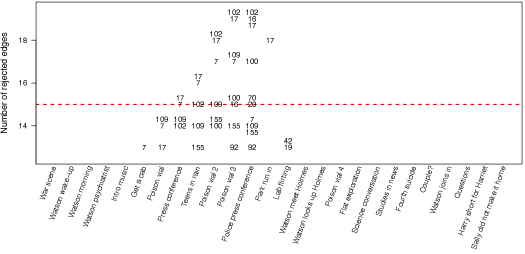
Figure 4: The $x$-axis displays the 26 scenes in the movie and the $y$-axis displays the number of rejected edges from Algorithm 1. The numbers correspond to the regions of interest (ROIs) in the brain. The ROIs correspond to frontal pole (7, 155), temporal fusiform cortex (16, 100), lingual gyrus (17), cingulate gyrus (19), cingulate gyrus (20), temporal pole (42), paracingulate gyrus (70), precuneus cortex (102), and postcentral gyrus (109).

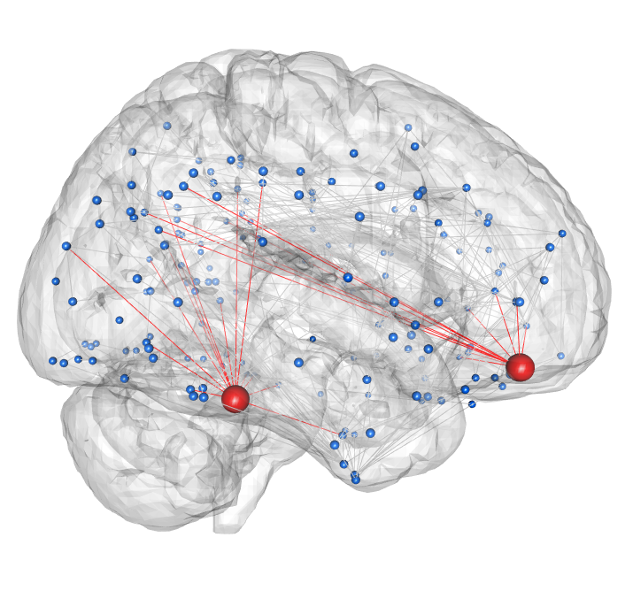
(a) Teens in rain scene

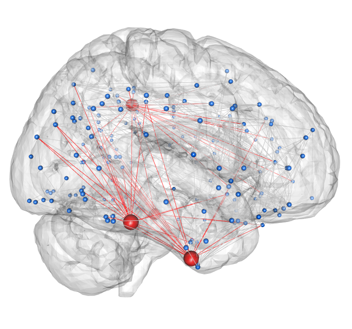
(b) Police press conference scene

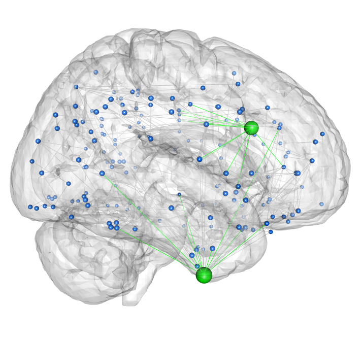
(c) Lab flirting scene

Figure 5: Sagittal snapshots of the rejected edges based on Algorithm 1. Panels (a)-(c) contain the snapshots for the “teens in rain”, “police press conference”, and “lab flirting” scenes, respectively. The red nodes and red edges are regions of interest that have more than 15 rejected edges. The grey edges are rejected edges from nodes that have no greater than 15 rejected edges. For (c), the green nodes and edges are regions of interest that have more than 12 rejected edges.

From Figure 4, we see that the rejected hub nodes (nodes that have more than 15 rejected edges) correspond to the frontal pole (7), temporal fusiform cortex (16, 100), lingual gyrus (17), and precuneus (102) regions of the brain. Many studies have suggested that the frontal pole plays significant roles in higher order cognitive operations such as decision making and moral reasoning (among others, Okuda et al. 2003). The fusiform cortex is linked to face and body recognition (see, Iaria et al. 2008, and the references therein). In addition, the lingual gyrus is known for its involvement in processing of visual information about parts of human faces (McCarthy et al. 1999). Thus, it is not surprising that both of these ROIs have more than 15 rejected edges since the brain images are collected while the subjects are exposed to an audio-visual movie stimulus.

Compared to the lingual gyrus, temporal fusiform cortex, and the frontal pole, the precuneus is the least well-understood brain literature in the current literature. We see from Figure 4 that the precuneus is the most connected ROI across many scenes. This is supported by the observation in Hagmann et al. (2008) where the precuneus serves as a hub region that is connected to many other parts of the brain. In recent years, Lerner et al. (2011) and Ames et al. (2015) conducted experiments where subjects were asked to listen to a story under an fMRI scanner. Their results suggest that the precuneus represents high-level concepts in the story, integrating feature information arriving from many different ROIs of the brain. Interestingly, we find that the precuneus has the highest number of rejected edges during the first half of the movie and that the number of rejected edges decreases significantly during the second half of the movie. Our results correspond well to the findings of Lerner et al. (2011) and Ames et al. (2015) in which the precuneus is active when the subjects comprehend the story. However, it also raises an interesting scientific question for future study: is the precuneus active only when the subjects are trying to comprehend the story, that is, once the story is understood, the precuneus is less active.

5 Theoretical Results

We establish uniform rates of convergence for the proposed estimators, and show that the testing procedure in Algorithm 1 is a uniformly valid test. We study the asymptotic regime in which $n$, $d$, and $s$ are allowed to increase. In the context of the Sherlock Holmes data set, $n$ is the total number of brain images obtained under the continuous stimulus, $d$ is the number of brain regions, and $s$ is the maximum number of connections for each brain region in the true stimulus-locked brain connectivity network. The current theoretical results assume that $Z$ is a random variable with continuous density. Our theoretical results can be easily generalized to the case when $\{Z_{i}\}_{i\in[n]}$ are fixed.

5.1 Theoretical Results on Parameter Estimation

Our proposed estimator involves a kernel function $K(\cdot)$: we require $K(\cdot)$ to be symmetric, bounded, unimodal, and compactly supported. More formally, for $l=1,2,3,4$,

$$\int K(u)du=1,\quad\int uK(u)du=0,\quad\int u^{l}K(u)du<\infty,\quad\int K^{l}(u)du<\infty.$$ (13)

In addition, we require the total variation of $K(\cdot)$ to be bounded, i.e., $\|K\|_{\mathrm{TV}}<\infty$, where $\|K\|_{\mathrm{TV}}=\int|\dot{K}|$. In other words, we require the kernel function to be a smooth function. The Epanechnikov kernel we consider in (5) for analyzing Sherlock data satisfies (13). A unimodal kernel function is extremely plausible in our setting: for instance, to estimate brain network in the “police press conference scene”, we expect the brain images within that scene to play a larger role than brain images that are far away from the scene. One practical limitation of the conditions on the kernel function is the symmetric kernel condition. When we are estimating a stimulus-locked brain network for a particular time point, the ideal case is to weight the previous images more heavily than the future brain images. The scientific reasoning is that there may be some time lag for information processing. In order to capture this effect, a more carefully designed kernel function is needed and it is out of the scope of this paper.

Next, we impose regularity conditions on the marginal density $f_{Z}(\cdot)$.

Assumption 1.

There exists a constant $\underline{f}_{Z}$ such that $\inf_{z\in[0,1]}\;f_{Z}(z)\geq\underline{f}_{Z}>0.$ Furthermore, $f_{Z}$ is twice continuously differentiable and that there exists a constant $\bar{f}_{Z}<\infty$ such that $\max\;\{\|f_{Z}\|_{\infty},\|\dot{f}_{Z}\|_{\infty},\|\ddot{f}_{Z}\|_{\infty}\}\leq\bar{f}_{Z}$.

Next, we impose smoothness assumptions on the inter-subject covariance matrix $\bm{\Sigma}(\cdot)$. Our theoretical results hold for any positive definite subject-specific covariance matrices $\mathbf{L}_{X}(z)$ and $\mathbf{L}_{Y}(z)$, since these matrices are treated as nuisance parameters.

Assumption 2.

There exists a constant $M_{\sigma}$ such that

$$\underset{z\in[0,1]}{\sup}\;\underset{j,k\in[d]}{\max}\;\max\left\{|\bm{\Sigma}_{jk}(z)|,|\dot{\bm{\Sigma}}_{jk}(z)|,|\ddot{\bm{\Sigma}}_{jk}(z)|\right\}\leq M_{\sigma}.$$

In other words, we assume that the inter-subject covariance matrices are smooth and do not change too rapidly in neighboring time points. This assumption clearly holds in a dynamic brain network where we expect the brain network to change smoothly over time. Assumptions 1 and 2 on $f(z)$ and $\bm{\Sigma}(z)$ are standard assumptions in the nonparametric statistics literature (see, for instance, Chapter 2 of Pagan & Ullah 1999).

The following theorem establishes the uniform rates of convergence for $\widehat{\bm{\Sigma}}(z)$.

Theorem 1.

Assume that $h=o(1)$ and that $\log^{2}(d/h)/(nh)=o(1)$. Under Assumptions 1-2, we have

$$\underset{z\in[0,1]}{\sup}\left\|\widehat{\bm{\Sigma}}(z)-\bm{\Sigma}(z)\right\|_{\max}=\mathcal{O}_{P}\left\{h^{2}+\sqrt{\frac{\log(d/h)}{nh}}\right\}.$$

Theorem 1 guarantees that our estimator always converges to the population parameter under the max norm, if the smoothing parameter $h$ goes to zero asymptotically. For instance, this will satisfy if $h=C\cdot n^{-1/5}$ for some constant $C>0$. The quantity ${\sup}_{{z\in[0,1]}}\|\widehat{\bm{\Sigma}}(z)-\bm{\Sigma}(z)\|_{\max}$ can be upper bounded by the summation of two terms: ${\sup}_{{z\in[0,1]}}\|\mathbb{E}[\widehat{\bm{\Sigma}}(z)]-\bm{\Sigma}(z)\|_{\max}$ and ${\sup}_{{z\in[0,1]}}\|\widehat{\bm{\Sigma}}(z)-\mathbb{E}[\widehat{\bm{\Sigma}}(z)]\|_{\max}$, which are known as the bias and variance terms, respectively, in the kernel smoothing literature (see, for instance, Chapter 2 of Pagan & Ullah 1999). The term $h^{2}$ on the upper bound corresponds to the bias term and the term $\sqrt{\log(d/h)/(nh)}$ corresponds to the variance term.

Next, we establish theoretical results for $\widehat{\bm{\Theta}}(z)$. Recall that the stimulus-locked brain connectivity network is encoded by the support of the inverse covariance matrix $\bm{\Theta}(z)$: $\bm{\Theta}_{jk}(z)=0$ if and only if the $j$th and $k$th brain regions are conditionally independent given all of the other brain regions. We consider the class of inverse covariance matrices:

$$\mathcal{U}_{s,M}=\left\{\bm{\Theta}\in\mathbb{R}^{d\times d}\mid\bm{\Theta}\succ 0,\;\|\bm{\Theta}\|_{2}\leq\rho,\;\underset{j\in[d]}{\max}\;\|\bm{\Theta}_{j}\|_{0}\leq s,\;\underset{j\in[d]}{\max}\;\|\bm{\Theta}_{j}\|_{1}\leq M\right\}.$$ (14)

Here, $\|\bm{\Theta}\|_{2}$ is the largest singular value of $\bm{\Theta}$ and $\|\bm{\Theta}_{j}\|_{0}$ is the number of non-zeros in $\bm{\Theta}_{j}$.

Brain connectivity networks are usually densely connected due to the intrinsic-neural and non-neuronal signals, such as background processing. Instead of assuming an overall sparse brain network, we assume that the stimulus-locked brain network $\bm{\Theta}(z)$ is sparse, and allow the intrinsic brain network unrelated to the stimulus to be dense. The sparsity assumption on stimulus-locked brain network is plausible in this setting since it characterizes brain activities that are specific to the stimulus. For instance, we may believe that only certain brain regions are active under cognitive process. The other conditions are satisfied since $\bm{\Theta}(z)$ is the inverse of a positive definite covariance matrix.

Given Theorem 1, the following corollary establishes the uniform rates of convergence for $\widehat{\bm{\Theta}}(z)$ using the CLIME estimator as defined in (6). It follows directly from the proof of Theorem 6 in Cai et al. (2011).

Corollary 1.

Assume that $\bm{\Theta}(z)\in\mathcal{U}_{s,M}$ for all $z\in[0,1]$. Let $\lambda\geq C\cdot\{h^{2}+\sqrt{\log(d/h)/(nh)}\}$ for $C>0$. Under the same conditions in Theorem 1,

$$\underset{z\in[0,1]}{\sup}\;\left\|\widehat{\bm{\Theta}}(z)-\bm{\Theta}(z)\right\|_{\max}=\mathcal{O}_{P}\left\{h^{2}+\sqrt{\frac{\log(d/h)}{nh}}\right\};$$ (15)

$$\underset{z\in[0,1]}{\sup}\;\underset{j\in[d]}{\max}\;\left\|\widehat{\bm{\Theta}}_{j}(z)-\bm{\Theta}_{j}(z)\right\|_{1}=\mathcal{O}_{P}\left[s\cdot\left\{h^{2}+\sqrt{\frac{\log(d/h)}{nh}}\right\}\right];$$ (16)

$$\underset{z\in[0,1]}{\sup}\;\underset{j\in[d]}{\max}\;\left\|\left\{\widehat{\bm{\Theta}}_{j}(z)\right\}^{T}\widehat{\bm{\Sigma}}(z)-\mathbf{e}_{j}\right\|_{\infty}=\mathcal{O}_{P}\left\{h^{2}+\sqrt{\frac{\log(d/h)}{nh}}\right\}.$$ (17)

In the real data analysis, Corollary 1 is helpful in terms of selecting the sparsity tuning parameter $\lambda$: it motivates a sparsity tuning parameter of the form $\lambda\geq C\cdot\{h^{2}+\sqrt{\log(d/h)/(nh)}\}$ to guarantee statistically consistent estimated stimulus-locked brain network. To select the constant $C$, we consider a sequence of number and select the appropriate $C$ using a data-driven cross-validation procedure in (7).

5.2 Theoretical Results on Topological Inference

In this section, we first show that the distribution of the test statistic $T_{E}$ can be approximated by the conditional $(1-\alpha)$-quantile of the bootstrap statistic $T^{B}_{E}$. Next, we show that the proposed testing method in Algorithm 1 is valid in the sense that the type I error can be controlled at a pre-specified level $\alpha$.

Recall from (12) the definition of $c(1-\alpha,E)$. The following theorem shows that the Gaussian multiplier bootstrap is valid for approximating the quantile of the test statistic $T_{E}$ in (10). Our results are based on the series of work on Gaussian approximation on multiplier bootstrap in high dimensions (see, e.g., Chernozhukov et al. 2013, 2014b). We see from (10) that $T_{E}$ involves taking the supremum over $z\in[0,1]$ and a dynamic edge set $E(z)$. Due to the dynamic edge set $E(z)$, existing theoretical results for the Gaussian multiplier bootstrap methods cannot be directly applied. We construct a novel Gaussian approximation result for the supreme of empirical processes of $T_{E}$ by carefully characterizing the capacity of the dynamic edge set $E(z)$.

Theorem 2.

Assume that $\sqrt{nh^{5}}+s\cdot\sqrt{nh^{9}}=o(1)$. In addition, assume that $s\sqrt{\log^{4}(d/h)/(nh^{2})}+\log^{22}(s)\cdot\log^{8}(d/h)/(nh)=o(1)$. Under the same conditions in Corollary 1, we have

$$\underset{n\rightarrow\infty}{\lim}\;\underset{\bm{\Theta}(\cdot)\in\mathcal{U}_{s,M}}{\sup}\;P_{\bm{\Theta}(\cdot)}\left\{T_{E}\geq c(1-\alpha,E)\right\}\leq\alpha.$$

Some of the scaling conditions are standard conditions in nonparametric estimation (Tsybakov 2009). The most notable scaling conditions are $s\sqrt{\log^{4}(d/h)/(nh^{2})}=o(1)$ and $\log^{22}(s)\cdot\log^{8}(d/h)/(nh)=o(1)$: these conditions arise from Gaussian approximation on multiplier bootstrap (Chernozhukov et al. 2013). These scaling conditions will hold asymptotically as long as the number of brain images $n$ is much larger than the maximum degree in the graph $s$. This corresponds well with the real data analysis where we expect only certain ROIs are active during information processing.

Recall the hypothesis testing problem in (8). We now show that the type I error of the proposed inferential method for testing the maximum degree of a time-varying graph can be controlled at a pre-specified level $\alpha$.

Theorem 3.

Assume that the same conditions in Theorem 2 hold. Under the null hypothesis in (8), we have

$$\underset{n\rightarrow\infty}{\lim}P_{\mathrm{null}}(\mathrm{Algorithm~{}\ref{al:stepdown}~{}rejects~{}the~{}null~{}hypothesis})\leq\alpha.$$

To study the power analysis of the proposed method, we define the signal strength of a precision matrix $\bm{\Theta}$ as

$$\text{Sig}_{\mathrm{deg}}(\bm{\Theta}):=\max_{{E^{\prime}\subseteq E(\bm{\Theta}),\text{Deg}(E)>k}}\min_{e\in E^{\prime}}|\bm{\Theta}_{e}|,$$ (18)

where $\text{Deg}(E)$ is the maximum degree of graph $G=(V,E)$. Under the alternative hypothesis in (8), $\mathrm{there\;exists\;a\;}z_{0}\in[0,1]\mathrm{\;such\;that\;}$ the maximum degree of the graph is greater than $k$. We define the parameter space under the alternative:

$$\mathcal{G}_{1}(\theta)=\Big{[}\bm{\Theta}(\cdot)\in\mathcal{U}_{s,M}\,\Big{|}\,\text{Sig}_{\mathrm{deg}}\{\bm{\Theta}(z_{0})\}\geq\theta\text{ for some $z_{0}\in[0,1]$}\Big{]}.$$ (19)

The following theorem presents the power analysis of Algorithm 1.

Theorem 4.

Assume that the same conditions in Theorem 2 hold and select the smoothing parameter such that $h=o(n^{-1/5})$. Under the alternative hypothesis in (8) and the assumption that $\theta\geq C\sqrt{\log(d/h)/nh}$, where $C$ is a fixed large constant, we have

$$\lim_{n\rightarrow\infty}\inf_{\bm{\Theta}\in\mathcal{G}_{1}(\theta)}\mathbb{P}_{\bm{\Theta}}(\mathrm{Algorithm~{}\ref{al:stepdown}~{}rejects~{}the~{}null~{}hypothesis})=1,$$ (20)

for any fixed $\alpha\in(0,1)$.

The signal strength condition defined in (24) is weaker than the typical minimal signal strength condition required on testing a single edge on a conditional independent graph, $\min_{e\in E(\bm{\Theta})}|\bm{\Theta}_{e}|$. The condition in (24) requires only that there exists a subgraph whose maximum degree is larger than $k$ and the minimal signal strength on that subgraph is above certain level. In our real data analysis, this requires only the edges for brain regions that are highly connected to many other brain regions to be strong, which is plausible since these regions should have high brain activity.

6 Discussion

We consider estimating stimulus-locked brain connectivity networks from data obtained under natural continuous stimuli. Due to lack of highly controlled experiments that remove all spontaneous and individual variations, the measured brain signal consists of not only stimulus-induced signal, but also intrinsic neural signal and non-neuronal signals that are subjects specific. Typical approach for estimating time-varying Gaussian graphical models will fail to estimate the stimulus-locked brain connectivity network accurately due to the presence of subject specific effects. By exploiting the experimental design aspect of the problem, we propose a simple approach to estimating stimulus-locked brain connectivity network. In particular, rather than calculating within-subject smoothed covariance matrix as in the typical approach for modeling time-varying Gaussian graphical models, we propose to construct the inter-subject smoothed covariance matrix instead, treating the subject specific effects as nuisance parameters.

To answer the scientific question on whether there are any brain regions that are connected to many other brain regions during the given stimulus, we propose an inferential method for testing the maximum degree of a stimulus-locked time-varying graph. In our analysis, we found that several interesting brain regions such as the fusiform cortex, lingual gyrus, and precuneus are highly connected. From the neuroscience literature, these brain regions are mainly responsible for high order cognitive operations, face and body recognition, and serve as control region that integrates information from other brain regions. We have also extended the proposed inferential framework to testing various topological graph structures. These are detailed in Appendix A.

The practical limitation of our proposed method is on the Gaussian assumption on the data. While we focus on the time-varying Gaussian graphical model in this paper, our framework can be extended to other types of time-varying graphical models such as the time-varying discrete graphical model or the time-varying nonparanormal graphical model (Kolar et al. 2010, Lu et al. 2015b). Another limitation is the independence assumption on the data across time points. All of our theoretical results can be generalized to the case when the data across time points are correlated, and we leave such generalization for future work.

Appendix A Inference on Topological Structure of Time-Varying Graph

In this section, we generalize Algorithm 1 in the main manuscript to testing various graph structures that satisfy the monotone graph property. In A.1, we briefly introduce some concepts on graph theory. These include the notion of isomorphism, graph property, monotone graph property, and critical edge set. In A.2, we provide a test statistic and an estimate of the quantile of the proposed test statistic using the Gaussian multiplier bootstrap. We then develop an algorithm to test the dynamic topological structure of a time-varying graph which satisfies the monotone graph property.

A.1 Graph Theory

Let $G=(V,E)$ be an undirected graph where $V=\{1,\ldots,d\}$ is a set of nodes and $E\subseteq V\times V$ is a set of edges connecting pairs of nodes. Let $\mathcal{G}$ be the set of all graphs with the same number of nodes. For any two graphs $G=(V,E)$ and $G^{\prime}=(V,E^{\prime})$, we write $G\subseteq G^{\prime}$ if $G$ is a subgraph of $G^{\prime}$, that is, if $E\subseteq E^{\prime}$. We start with introducing some concepts on graph theory (see, for instance, Chapter 4 of Lovász 2012).

Definition 1.

Two graphs $G=(V,E)$ and $G^{\prime}=(V,E^{\prime})$ are said to be isomorphic if there exists permutations $\pi:V\rightarrow V$ such that $(j,k)\in E$ if and only if $\{\pi(j),\pi(k)\}\in E^{\prime}$.

The notion of isomorphism is used in the graph theory literature to quantify whether two graphs have the same topological structure, up to any permutation of the vertices (see Chapter 1.2 of Bondy & Murty 1976). We provide two concrete examples on the notion of isomorphism in Figure 6.

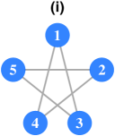
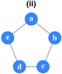
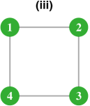
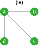
Figure 6: Graphs (i) and (ii) are isomorphic. Graphs (iii) and (iv) are not isomorphic.

Next, we introduce the notion of graph property. A graph property is a property of graphs that depends only on the structure of the graphs, that is, a graph property is invariant under permutation of vertices. A formal definition is given as follows.

Definition 2.

For two graphs $G$ and $G^{\prime}$ that are isomorphic, a graph property is a function $\mathcal{P}:\mathcal{G}\rightarrow\{0,1\}$ such that $\mathcal{P}(G)=\mathcal{P}(G^{\prime})$. A graph $G$ satisfies the graph property $\mathcal{P}$ if $\mathcal{P}(G)=1$.

Some examples of graph property are that the graph is connected, the graph has no more than $k$ connected components, the maximum degree of the graph is larger than $k$, the graph has no more than $k$ isolated nodes, the graph contains a clique of size larger than $k$, and the graph contains a triangle. For instance, the two graphs in Figures 6(i) and 6(ii) are isomorphic and satisfy the graph property of being connected.

Definition 3.

For two graphs $G\subseteq G^{\prime}$, a graph property $\mathcal{P}$ is monotone if $\mathcal{P}(G)=1$ implies that $\mathcal{P}(G^{\prime})=1$.

In other words, we say that a graph property is monotone if the graph property is preserved under the addition of new edges. Many graph property that are of interest such as those given in the paragraph immediately after Definition 2 are monotone. In Figure 7, we present several examples of graph property that are monotone by showing that adding additional edges to the graph does not change the graph property. For instance, we see from Figure 7(a) that the existing graph with gray edges are connected. Adding the red edges to the existing graph, the graph remains connected and therefore the graph property is monotone. Another example is the graph with maximum degree at least three as in Figure 7(c). We see that adding the red dash edges to the graph preserves the graph property of having maximum degree at least three.

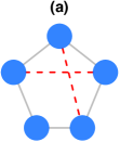
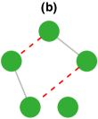
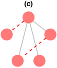
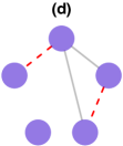
Figure 7: Some examples on graph property that are monotone. The gray edges are the original edges and the red dash edges are additional edges added to the existing graph. (a) Graph that is connected. (b) Graph that has no more than three connected components. (c) Graph with maximum degree at least three. (d) Graph with no more than two isolated nodes. Adding the red dash edges to the existing graphs does not change the graph property.

For a given graph $G=(V,E)$, we define the class of edge sets satisfying the graph property $\mathcal{P}$ as

$$\mathscr{P}=\{E\subseteq V\times V\mid\mathcal{P}(G)=1\}.$$ (21)

Finally, we introduce the notion of critical edge set in the following definition.

Definition 4.

Given any edge set $E\subseteq V\times V$, we define the critical edge set of $E$ for a given monotone graph property $\mathcal{P}$ as

$$\mathcal{C}(E,\mathcal{P})=\{e\mid e\not\in E,\;\mathrm{there\;exists\;}E^{\prime}\supseteq E\mathrm{\;such\;that\;}E^{\prime}\in\mathscr{P}\text{ and }E^{\prime}\backslash\{e\}\notin\mathscr{P}\}.$$ (22)

For a given monotone graph property $\mathcal{P}$, the critical edge set is the set of edges that will change the graph property of the graph once added to the existing graph. We provide two examples in Figure 8. Suppose that $\mathcal{P}$ is the graph property of being connected. In Figure 8(a), we see that the graph is not connected, and thus $\mathcal{P}(G)=0$. Adding any of the red dash edges in Figure 8(b) changes $\mathcal{P}(G)=0$ to $\mathcal{P}(G)=1$.

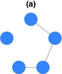
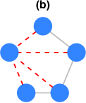
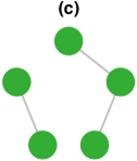
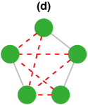
Figure 8: Let $\mathcal{P}$ be the graph property of being connected. Gray edges are the original edges of a graph $G$ and the red dash edges are the critical edges that will change the graph property from $\mathcal{P}(G)=0$ to $\mathcal{P}(G)=1$. (a) The graph satisfies $\mathcal{P}(G)=0$. (b) The graph property changes from $\mathcal{P}(G)=0$ to $\mathcal{P}(G)=1$ if some red dash edges are added to the graph. (c) The graph satisfies $\mathcal{P}(G)=0$. (d) The graph property changes from $\mathcal{P}(G)=0$ to $\mathcal{P}(G)=1$ if some red dash edges are added to the existing graph.

A.2 An Algorithm for Topological Inference

Throughout the rest of the paper, we denote $G(z)=\{V,E(z)\}$ as the graph at $Z=z$. We consider hypothesis testing problem of the form

$$\begin{split}&H_{0}:\mathcal{P}\{G(z)\}=0\mathrm{\;for\;all\;}z\in[0,1]\\ &H_{1}:\mathrm{there\;exists\;a\;}z_{0}\in[0,1]\mathrm{\;such\;that\;}\mathcal{P}\{G(z_{0})\}=1,\end{split}$$ (23)

where $G(\cdot)$ is the true underlying graph and $\mathcal{P}$ is a given monotone graph property as defined in Definition 3. We provide two concrete examples of the hypothesis testing problem in (23).

Example 1.

Number of connected components:

$$\begin{split}&H_{0}:\mathrm{\;for\;all\;}z\in[0,1],\mathrm{\;the\;number\;of\;connected\;components\;is\;greater\;than\;}k,\\ &H_{1}:\mathrm{\;there\;exists\;a\;}z_{0}\in[0,1]\mathrm{\;such\;that\;the\;number\;of\;connected\;components\;is\;not\;greater\;than\;}k.\\ \end{split}$$

Example 2.

Maximum degree of the graph:

$$\begin{split}&H_{0}:\mathrm{\;for\;all\;}z\in[0,1],\mathrm{\;the\;maximum\;degree\;of\;the\;graph\;is\;not\;greater\;than\;}k,\\ &H_{1}:\mathrm{\;there\;exists\;a\;}z_{0}\in[0,1]\mathrm{\;such\;that\;the\;maximum\;degree\;of\;the\;graph\;is\;greater\;than\;}k.\\ \end{split}$$

We now propose an algorithm to test the topological structure of a time-varying graph. The proposed algorithm is very general and is able to test the hypothesis problem of the form in (23). Our proposed algorithm is motivated by the step-down algorithm in Romano & Wolf (2005) for testing multiple hypothesis simultaneously. The main crux of our algorithm is as follows. By Definition 4, the critical edge set $\mathcal{C}\{E_{t-1}(z),\mathcal{P}\}$ contains edges that may change the graph property from $\mathcal{P}\{G(z)\}=0$ to $\mathcal{P}\{G(z)\}=1$. Thus, at the $t$-th iteration of the proposed algorithm, it suffices to test whether the edges on the critical edge set $\mathcal{C}\{E_{t-1}(z),\mathcal{P}\}$ are rejected. Let $E_{t}(z)=E_{t-1}(z)\;\cup\;\mathcal{R}(z)$, where $\mathcal{R}(z)$ is the rejected edge set from the critical edge set $\mathcal{C}\{E_{t-1}(z),\mathcal{P}\}$. Since $\mathcal{P}$ is a monotone graph property, if there exists a $z_{0}\in[0,1]$ such that $E_{t}(z_{0})\in\mathscr{P}$, we directly reject the null hypothesis $H_{0}:\mathcal{P}\{G(z)\}=0$ for all $z$. This is due to the definition of monotone graph property that adding more edges does not change the graph property. If $E_{t}(z_{0})\notin\mathscr{P}$, we repeat this process until the null hypothesis is rejected or no more edges in the critical edge set are rejected. We summarize the procedure in Algorithm 2.

Algorithm 2 Dynamic skip-down method.

Input: A monotone graph property $\mathcal{P}$; $\widehat{\bm{\Theta}}^{\mathrm{de}}(z)$ for $z\in[0,1]$.
Initialize: $t=1$; $E_{0}(z)=\emptyset$ for $z\in[0,1]$.
Repeat:

1. Compute the critical edge set $\mathcal{C}\{E_{t-1}(z),\mathcal{P}\}$ for $z\in[0,1]$ and the conditional quantile $c\{1-\alpha,\mathcal{C}(E_{t-1},\mathcal{P})\}=\inf\left(t\in\mathbb{R}\mid P[T^{B}_{\mathcal{C}(E_{t-1},\mathcal{P})}\leq t\mid\{(\bm{X}_{i},\bm{Y}_{i},Z_{i})\}_{i\in[n]}]\geq 1-\alpha\right)$, where $T^{B}_{\mathcal{C}(E_{t-1},\mathcal{P})}$ is the bootstrap statistic defined in (11) with the maximum taken over the edge set $\mathcal{C}\{E_{t-1}(z),\mathcal{P}\}$.

2. Construct the rejected edge set

   $$\mathcal{R}(z)=\left[e\in\mathcal{C}\{E_{t-1}(z),\mathcal{P}\}\mid\sqrt{nh}\cdot|\widehat{\bm{\Theta}}_{e}^{\mathrm{de}}(z)|\cdot\sum_{i\in[n]}K_{h}(Z_{i}-z)/n>c\{1-\alpha,\mathcal{C}(E_{t-1},\mathcal{P})\}\right].$$

3. Update the rejected edge set $E_{t}(z)\leftarrow E_{t-1}(z)\cup\mathcal{R}(z)$ for $z\in[0,1]$.

4. $t\leftarrow t+1$.

Until: There exists a $z_{0}\in[0,1]$ such that $E_{t}(z_{0})\in\mathscr{P}$, or $E_{t}(z)=E_{t-1}(z)$ for $z\in[0,1]$.

Output: $\psi_{\alpha}=1$ if there exists a $z_{0}\in[0,1]$ such that $E_{t}(z_{0})\in\mathscr{P}$ and $\psi_{\alpha}=0$ otherwise.

Finally, we generalize the theoretical results in Theorems 3 and 4 to the general testing procedure in Algorithm 2. Given a monotone graph property $\mathcal{P}$, let

$$\mathcal{G}_{0}=(\bm{\Theta}(\cdot)\in\mathcal{U}_{s,M}\mid\mathcal{P}[G\{\bm{\Theta}(z)\}]=0\mathrm{\;for\;all\;}z\in[0,1]).$$

We now show that the type I error of the proposed inferential method in Algorithm 2 can be controlled at a pre-specified level $\alpha$.

Theorem 5.

Under the same conditions in Theorem 2, we have

$$\underset{n\rightarrow\infty}{\lim}\underset{\bm{\Theta}(\cdot)\in\mathcal{G}_{0}}{\sup}P_{\bm{\Theta}(\cdot)}\left(\psi_{\alpha}=1\right)\leq\alpha.$$

In order to study the power analysis for testing graph structure that satisfies the monotone graph property, we define signal strength of a precision matrix $\bm{\Theta}$ as

$$\text{Sig}(\bm{\Theta}):=\max_{{E^{\prime}\subseteq E(\bm{\Theta}),\mathcal{P}(E^{\prime})=1}}\min_{e\in E^{\prime}}|\bm{\Theta}_{e}|.$$ (24)

Under $H_{1}:\mathrm{there\;exists\;a\;}z_{0}\in[0,1]\mathrm{\;such\;that\;}\mathcal{P}\{G(z_{0})\}=1$, we define the parameter space

$$\mathcal{G}_{1}(\theta;\mathcal{P})=\Big{(}\bm{\Theta}(\cdot)\in\mathcal{U}_{s,M}\,\Big{|}\,\mathcal{P}[G\{\bm{\Theta}(z_{0})\}]=1\text{ and }\text{Sig}\{\bm{\Theta}(z_{0})\}\geq\theta\text{ for some $z_{0}\in[0,1]$}\Big{)}.$$ (25)

Again, we emphasize that the signal strength defined in (24) is weaker than the typical minimal signal strength for testing a single edge in a graph $\min_{e\in E(\bm{\Theta})}|\bm{\Theta}_{e}|$. $\text{Sig}(\bm{\Theta})$ only requires that there exists a subgraph satisfying the property of interest such that the minimal signal strength on that subgraph is above certain level. For example, for $\mathcal{P}(G)=1$ if and only if $G$ is connected, it suffices for $\bm{\Theta}$ belongs to $\mathcal{G}_{1}(\theta;\mathcal{P})$ if the minimal signal strength on a spanning tree is larger than $\theta$. The following theorem presents the power analysis of our test.

Theorem 6.

Assume that the same conditions in Theorem 2 hold and select the smoothing parameter $h=o(1/n^{-1/5})$. Assume that $\theta\geq C\sqrt{\log(dn)}/n^{2/5}$ for some sufficiently large constant $C$. Under the alternative hypothesis $H_{1}:\mathcal{P}(G)=1$ in (23), we have

$$\lim_{n\rightarrow\infty}\inf_{\bm{\Theta}\in\mathcal{G}_{1}(\theta;\mathcal{P})}\mathbb{P}_{\bm{\Theta}}(\psi_{\alpha}=1)=1$$ (26)

for any fixed $\alpha\in(0,1)$.

Thus, we have shown in Theorem 6 that the power of the proposed inferential method increases to one asymptotically.

Appendix B A $U$-Statistic Type Estimator

The main manuscript primarily concerns the case when there are two subjects. In this section, we present a $U$-statistic type inter-subject covariance to accommodate the case when there are more than two subjects. First, we note that the same natural stimuli is given to all subjects. This motivates the following statistical model for each $Z=z$:

$$\bm{X}^{(\ell)}=\bm{S}+\bm{E}^{(\ell)},~{}~{}\bm{S}|Z=z\sim N_{d}\{\mathbf{0},\bm{\Sigma}(z)\},~{}~{}\bm{E}^{(\ell)}|Z=z\sim N_{d}\{\mathbf{0},\bm{L}^{(\ell)}(z)\},$$

where $\bm{X}^{(\ell)}$, $\bm{E}^{(\ell)}$, and $\bm{L}^{(\ell)}(z)$ are the data, subject specific effect, and the covariance matrix for the subject specific effect for the $\ell$th subject, respectively. Suppose that there $N$ subjects. Then, the following $U$-statistic type inter-subject covariance matrix can be constructed to estimate $\bm{\Sigma}(z)$:

$$\widehat{\mathbf{\Sigma}}_{U}(z)=\frac{1}{{N\choose 2}}\sum_{1\leq\ell<\ell^{\prime}\leq N}\left[\frac{\sum_{i\in[n]}K_{h}(Z_{i}-z)\bm{X}_{i}^{(\ell)}\{\bm{X}_{i}^{(\ell^{\prime})}\}^{T}}{\sum_{i\in[n]}K_{h}(Z_{i}-z)}\right].$$ (27)

We leave the theoretical analysis of the above estimator for future work.

Appendix C Preliminaries

In this section, we define some notation that will be used throughout the Appendix. Let $[n]$ denote the set $\{1,\ldots,n\}$ and let $[d]$ denote the set $\{1,\ldots,d\}$. For two scalars $a,b$, we define $a\vee b=\max(a,b)$. We denote the $\ell_{q}$-norm for the vector $\mathbf{v}$ as $\|\mathbf{v}\|_{q}=(\sum_{j\in[d]}|v_{j}|^{q})^{1/q}$ for $1\leq q<\infty$. In addition, we let $\mathrm{supp}(\mathbf{v})=\{j:v_{j}\neq 0\}$, $\|\mathbf{v}\|_{0}=|\mathrm{supp}(\mathbf{v})|$, and $\|\mathbf{v}\|_{\infty}={\max}_{j\in[d]}\;|v_{j}|$, where $|\mathrm{supp}(\mathbf{v})|$ is the number of non-zero elements in $\mathbf{v}$. For a matrix $\mathbf{A}\in\mathbb{R}^{n_{1}\times n_{2}}$, we denote the $j$th column as $\mathbf{A}_{j}$. We denote the Frobenius norm of $\mathbf{A}$ by $\|\mathbf{A}\|_{F}^{2}=\sum_{i\in[n_{1}]}\sum_{j\in[n_{2}]}A_{ij}^{2}$, the max norm $\|\mathbf{A}\|_{\max}=\max_{i\in[n_{1}],j\in[n_{2}]}|A_{ij}|$, and the operator norm $\|\mathbf{A}\|_{2}=\sup_{\|\mathbf{v}\|_{2}=1}\;\|\mathbf{A}\mathbf{v}\|_{2}$. Given a function $f$, let $\dot{f}$ and $\ddot{f}$ be the first and second-order derivatives, respectively. For $1\leq p<\infty$, let $\|f\|_{p}=(\int f^{p})^{1/p}$ denote the $L_{p}$ norm of $f$ and let $\|f\|_{\infty}=\sup_{x}|f(x)|$. The total variation of $f$ is defined as $\|f\|_{\mathrm{TV}}=\int|\dot{f}|$. We use the Landau symbol $a_{n}=\mathcal{O}(b_{n})$ to indicate the existence of a constant $C>0$ such that $a_{n}\leq C\cdot b_{n}$ for two sequences $a_{n}$ and $b_{n}$. We write $a_{n}=o(b_{n})$ if ${\lim}_{n\rightarrow\infty}\;a_{n}/b_{n}\rightarrow 0$. Let $C,C_{1},C_{2},\ldots$ be generic constants whose values may vary from line to line.

Let

$$\mathbb{P}_{n}(f)=\frac{1}{n}\sum_{i\in[n]}f(X_{i})\qquad\mathrm{and}\qquad\mathbb{G}_{n}(f)=\sqrt{n}\cdot[\mathbb{P}_{n}(f)-\mathbb{E}\{f(X_{i})\}].$$ (28)

For notational convenience, for fixed $j,k\in[d]$, let

$$g_{z,jk}(Z_{i},X_{ij},Y_{ik})=K_{h}(Z_{i}-z)X_{ij}Y_{ik},\qquad\qquad w_{z}(Z_{i})=K_{h}(Z_{i}-z),$$ (29)

$$q_{z,jk}(Z_{i},X_{ij},Y_{ik})=g_{z,jk}(Z_{i},X_{ij},Y_{ik})-\mathbb{E}\{g_{z,jk}(Z,X_{j},Y_{k})\},$$ (30)

and let

$$k_{z}(Z_{i})=w_{z}(Z_{i})-\mathbb{E}\{w_{z}(Z)\}.$$ (31)

Recall from 5 that $K(\cdot)$ can be any symmetric kernel function that satisfies (13) and that $K_{h}(Z_{i}-z)=K\{(Z_{i}-z)/h\}/h$. By the definition of $\widehat{\bm{\Sigma}}(z)$ in (27), we have

$$\widehat{\bm{\Sigma}}_{jk}(z)=\frac{\sum_{i\in[n]}g_{z,jk}(Z_{i},X_{ij},Y_{ik})}{\sum_{i\in[n]}w_{z}(Z_{i})}=\frac{\mathbb{P}_{n}(g_{z,jk})}{\mathbb{P}_{n}(w_{z})}.$$ (32)

In addition, let

$$J_{z,jk}^{(1)}(Z_{i},\bm{X}_{i},\bm{Y}_{i})=\sqrt{h}\cdot\left\{\bm{\Theta}_{j}(z)\right\}^{T}\cdot\left[K_{h}(Z_{i}-z)\bm{X}_{i}\bm{Y}_{i}^{T}-\mathbb{E}\left\{K_{h}(Z-z)\bm{X}\bm{Y}^{T}\right\}\right]\cdot\bm{\Theta}_{k}(z),$$ (33)

$$\begin{split}J_{z,jk}^{(2)}(Z_{i})&=\sqrt{h}\cdot\left\{\bm{\Theta}_{j}(z)\right\}^{T}\cdot\left[K_{h}(Z_{i}-z)-\mathbb{E}\left\{K_{h}(Z-z)\right\}\right]\cdot\bm{\Sigma}(z)\cdot\bm{\Theta}_{k}(z),\end{split}$$ (34)

$$\begin{split}J_{z,jk}(Z_{i},\bm{X}_{i},\bm{Y}_{i})=J_{z,jk}^{(1)}(Z_{i},\bm{X}_{i},\bm{Y}_{i})-J_{z,jk}^{(2)}(Z_{i}),\end{split}$$ (35)

and let

$$W_{z,jk}(Z_{i},X_{ij},Y_{ik})=\sqrt{h}\cdot\left\{K_{h}(Z_{i}-z)X_{ij}Y_{ik}-K_{h}(Z_{i}-z)\bm{\Sigma}_{jk}(z)\right\}.$$ (36)

For two functions $f$ and $g$, we define its convolution as

$$(f*g)(x)=\int f(x-z)g(z)dz.$$ (37)

In our proofs, we will use the following property of the derivative of a convolution

$$\frac{\partial}{\partial x}(f*g)=\frac{\partial f}{\partial x}*g.$$ (38)

Finally, our proofs use the following inequality

$$\int_{0}^{b_{1}}\sqrt{\log(b_{2}/\epsilon)}d\epsilon\leq\sqrt{b_{1}}\cdot\sqrt{\int_{0}^{b_{1}}\log(b_{2}/\epsilon)d\epsilon}=b_{1}\cdot\sqrt{1+\log(b_{2}/b_{1})},$$ (39)

where the first inequality holds by an application of Jensen’s inequality.

Appendix D Proof of Results in 5.1

In this section, we establish the uniform rate of convergence for $\widehat{\bm{\Sigma}}(z)$ and $\widehat{\bm{\Theta}}(z)$ over $z\in[0,1]$. To prove Theorem 1, we first observe that

$$\underset{z\in[0,1]}{\sup}\left\|\widehat{\bm{\Sigma}}(z)-\bm{\Sigma}(z)\right\|_{\max}\leq\underset{z\in[0,1]}{\sup}\;\underset{j,k\in[d]}{\max}\;\left|\widehat{\bm{\Sigma}}_{jk}(z)-\mathbb{E}\left\{\widehat{\bm{\Sigma}}_{jk}(z)\right\}\right|+\underset{z\in[0,1]}{\sup}\;\underset{j,k\in[d]}{\max}\;\left|\mathbb{E}\left\{\widehat{\bm{\Sigma}}_{jk}(z)\right\}-\bm{\Sigma}_{jk}(z)\right|.$$ (40)

The first term is known as the variance term and the second term is known as the bias term in the kernel smoothing literature (see, for instance, Chapter 2 of Pagan & Ullah 1999). Both the variance and bias terms involve evaluating the quantity $\mathbb{E}\{\widehat{\bm{\Sigma}}_{jk}(z)\}$. From (32), we see that $\widehat{\bm{\Sigma}}_{jk}(z)$ involves the quotient of two averages and it is not straightforward to evaluate its expectation. The following lemma quantifies $\mathbb{E}\{\widehat{\bm{\Sigma}}_{jk}(z)\}$ in terms of the expectations of its numerator and its denominator.

Lemma 1.

Under the following conditions

$$\left|\frac{\mathbb{G}_{n}(w_{z})}{\sqrt{n}\cdot\mathbb{E}\left\{\mathbb{P}_{n}(w_{z})\right\}}\right|<1\qquad\mathrm{and}\qquad\mathbb{E}\left\{\mathbb{P}_{n}(w_{z})\right\}\neq 0,$$ (41)

we have

$$\mathbb{E}\left\{\widehat{\bm{\Sigma}}_{jk}(z)\right\}=\frac{\mathbb{E}\left\{\mathbb{P}_{n}(g_{z,jk})\right\}}{\mathbb{E}\left\{\mathbb{P}_{n}(w_{z})\right\}}+\frac{1}{n}\mathcal{O}\left[\mathbb{E}\Big{\{}\mathbb{G}_{n}(w_{z})\cdot\mathbb{G}_{n}(g_{z,jk})\Big{\}}+\mathbb{E}\left\{\mathbb{G}_{n}^{2}(g_{z,jk})\right\}\right].$$ (42)

We note that (42) only holds under the two conditions in (41). In the proof of Theorem 1, we will show that the two conditions in (41) hold for $n$ sufficiently large. To obtain upper bounds for the bias and variance terms in (40), we use the following intermediate lemmas.

Lemma 2.

Assume that $h=o(1)$. Under Assumptions 1-2, we have

$$\underset{z\in[0,1]}{\sup}\;\underset{j,k\in[d]}{\max}\;\Big{|}\mathbb{E}\{\mathbb{P}_{n}(g_{z,jk})\}-f_{Z}(z)\bm{\Sigma}_{jk}(z)\Big{|}=\mathcal{O}(h^{2}),$$ (43)

$$\underset{z\in[0,1]}{\sup}\;\Big{|}\mathbb{E}\{\mathbb{P}_{n}(w_{z})\}-f_{Z}(z)\Big{|}=\mathcal{O}(h^{2}),$$ (44)

$$\underset{z\in[0,1]}{\sup}\;\underset{j,k\in[d]}{\max}\;\frac{1}{n}\left|\mathbb{E}\Big{\{}\mathbb{G}_{n}(g_{z,jk})\cdot\mathbb{G}_{n}(w_{z})\Big{\}}\right|=\mathcal{O}\left(\frac{1}{nh}\right),$$ (45)

and

$$\underset{z\in[0,1]}{\sup}\;\frac{1}{n}\mathbb{E}\Big{\{}\mathbb{G}_{n}^{2}(w_{z})\Big{\}}=\mathcal{O}\left(\frac{1}{nh}\right).$$ (46)

Lemma 3.

Assume that $h=o(1)$ and $\log^{2}(d/h)/(nh)=o(1)$. Under Assumptions 1-2, there exists a universal constant $C>0$ such that

$$\underset{z\in[0,1]}{\sup}\;\underset{j,k\in[d]}{\max}\;\Big{|}\mathbb{G}_{n}(w_{z})\vee\mathbb{G}_{n}(g_{z,jk})\Big{|}\leq C\cdot\sqrt{\frac{\log(d/h)}{h}},$$ (47)

with probability at least $1-3/d$.

The proofs of Lemmas 1-3 are deferred to Sections 1-3, respectively. We now provide a proof of Theorem 1.

D.1 Proof of Theorem 1

Recall from (40) that

$$\begin{split}\underset{z\in[0,1]}{\sup}\left\|\widehat{\bm{\Sigma}}(z)-\bm{\Sigma}(z)\right\|_{\max}&\leq\underset{z\in[0,1]}{\sup}\;\underset{j,k\in[d]}{\max}\;\left|\widehat{\bm{\Sigma}}_{jk}(z)-\mathbb{E}\left\{\widehat{\bm{\Sigma}}_{jk}(z)\right\}\right|+\underset{z\in[0,1]}{\sup}\;\underset{j,k\in[d]}{\max}\;\left|\mathbb{E}\left\{\widehat{\bm{\Sigma}}_{jk}(z)\right\}-\bm{\Sigma}_{jk}(z)\right|\\ &=I_{1}+I_{2}.\end{split}$$

It suffices to obtain upper bounds for $I_{1}$ and $I_{2}$.

We first verify that the two conditions in (41) hold. By Lemma 2, we have

$$\Big{|}\mathbb{E}\{\mathbb{P}_{n}(w_{z})\}\Big{|}=\mathcal{O}(h^{2})+f_{Z}(z)\geq\underline{f}_{Z}(z)>0,$$

where the last inequality follows from Assumption 1. Moreover,

$$\begin{split}\left|\frac{\mathbb{G}_{n}(w_{z})}{\sqrt{n}\cdot\mathbb{E}\left\{\mathbb{P}_{n}(w_{z})\right\}}\right|&\leq C\cdot\frac{1}{\sqrt{n}}|\mathbb{G}_{n}(w_{z})|\cdot\frac{1}{f_{Z}(z)+\mathcal{O}(h^{2})}\\ &\leq C_{1}\cdot\sqrt{\frac{\log(d/h)}{nh}}\cdot\frac{1}{f_{Z}(z)+\mathcal{O}(h^{2})}\\ &<1,\end{split}$$

for sufficiently large $n$, where the first inequality is obtained by an application of Lemma 2, the second inequality is obtained by an application of Lemma 3, and the last inequality is obtained by the scaling assumptions $h=o(1)$ and $\log(d/h)/(nh)=o(1)$.

Upper bound for $I_{1}$: By (55) in the proof of Lemma 1, we have

$$\widehat{\bm{\Sigma}}_{jk}(z)=\frac{\mathbb{G}_{n}(g_{z,jk})}{\sqrt{n}\mathbb{E}\left\{\mathbb{P}_{n}(w_{z})\right\}}+\frac{\mathbb{E}\{\mathbb{P}_{n}(g_{z,jk})\}}{\mathbb{E}\left\{\mathbb{P}_{n}(w_{z})\right\}}-\frac{\mathbb{G}_{n}(w_{z})\mathbb{E}\{\mathbb{P}_{n}(g_{z,jk})\}}{\sqrt{n}\mathbb{E}^{2}\{\mathbb{P}_{n}(w_{z})\}}+\frac{1}{n}\mathcal{O}\left[\Big{\{}\mathbb{G}_{n}(w_{z})\mathbb{G}_{n}(g_{j,zk})\Big{\}}+\mathbb{G}_{n}^{2}(g_{z,jk})\right].$$

Thus, by Lemma 1, we have

$$\begin{split}I_{1}&=\underset{z\in[0,1]}{\sup}\;\underset{j,k\in[d]}{\max}\;\left|\underbrace{\frac{\mathbb{G}_{n}(g_{z,jk})}{\sqrt{n}\cdot\mathbb{E}\left\{\mathbb{P}_{n}(w_{z})\right\}}}_{I_{11}}-\underbrace{\frac{\mathbb{G}_{n}(w_{z})\cdot\mathbb{E}\{\mathbb{P}_{n}(g_{z,jk})\}}{\sqrt{n}\cdot\mathbb{E}^{2}\{\mathbb{P}_{n}(w_{z})\}}}_{I_{12}}+I_{13}\right|\\ &\leq\underset{z\in[0,1]}{\sup}\;\underset{j,k\in[d]}{\max}\;\left\{|I_{11}|+|I_{12}|+|I_{13}|\right\},\end{split}$$ (48)

where $I_{13}=\mathcal{O}[\{\mathbb{G}_{n}(w_{z})\mathbb{G}_{n}(g_{j,zk})\}+\mathbb{G}_{n}^{2}(g_{z,jk})+\mathbb{E}\{\mathbb{G}_{n}(w_{z})\cdot\mathbb{G}_{n}(g_{j,zk})\}+\mathbb{E}\{\mathbb{G}_{n}^{2}(g_{z,jk})\}]/n$.

We now provide upper bounds for $I_{11}$, $I_{12}$, and $I_{13}$. By an application of Lemmas 2 and 3, we obtain

$$\underset{z\in[0,1]}{\sup}\;\underset{j,k\in[d]}{\max}\;|I_{11}|\leq n^{-1/2}\cdot\underset{z\in[0,1]}{\sup}\;\underset{j,k\in[d]}{\max}\;\left|\frac{\mathbb{G}_{n}(g_{z,jk})}{f_{Z}(z)+\mathcal{O}(h^{2})}\right|\leq C\cdot\sqrt{\frac{\log(d/h)}{nh}}.$$ (49)

Similarly, we have

$$\underset{z\in[0,1]}{\sup}\;\underset{j,k\in[d]}{\max}\;|I_{12}|\leq n^{-1/2}\cdot\underset{z\in[0,1]}{\sup}\;\underset{j,k\in[d]}{\max}\;\left|\frac{\mathbb{G}_{n}(g_{z,jk})\{f_{Z}(z)\bm{\Sigma}_{jk}(z)+\mathcal{O}(h^{2})\}}{\{f_{Z}(z)+\mathcal{O}(h^{2})\}^{2}}\right|\leq C\cdot\sqrt{\frac{\log(d/h)}{nh}}.$$ (50)

For $I_{13}$, we have

$$\begin{split}\underset{z\in[0,1]}{\sup}\;\underset{j,k\in[d]}{\max}\;|I_{13}|&\leq\underset{z\in[0,1]}{\sup}\;\underset{j,k\in[d]}{\max}\;\left|\frac{1}{n}\mathcal{O}\left[\Big{\{}\mathbb{G}_{n}(w_{z})\cdot\mathbb{G}_{n}(g_{z,jk})\Big{\}}+\mathbb{G}_{n}^{2}(g_{z,jk})\right]\right|+\mathcal{O}\left(\frac{1}{nh}\right)\\ &\leq C\cdot{\frac{\log(d/h)}{nh}}+\mathcal{O}\left(\frac{1}{nh}\right)\\ &\leq C\cdot{\frac{\log(d/h)}{nh}},\end{split}$$ (51)

where the first and second inequalities follow from Lemmas 2 and 3, respectively. Combining (49), (50), and (51), we have

$$I_{1}\leq C\cdot\sqrt{\frac{\log(d/h)}{nh}},$$ (52)

with probability at least $1-3/d$.

Upper bound for $I_{2}$: By Lemmas 1 and 2, we have

$$\begin{split}I_{2}&=\underset{z\in[0,1]}{\sup}\;\underset{j,k\in[d]}{\max}\;\left|\frac{\mathbb{E}\left\{\mathbb{P}_{n}(g_{z,jk})\right\}}{\mathbb{E}\left\{\mathbb{P}_{n}(w_{z})\right\}}-\bm{\Sigma}_{jk}(z)+\frac{1}{n}\mathcal{O}\left[\mathbb{E}\Big{\{}\mathbb{G}_{n}(w_{z})\cdot\mathbb{G}_{n}(g_{z,jk})\Big{\}}+\mathbb{E}\left\{\mathbb{G}_{n}^{2}(g_{z,jk})\right\}\right]\right|\\ &\leq\underset{z\in[0,1]}{\sup}\;\underset{j,k\in[d]}{\max}\;\left|\frac{f_{Z}(z)\bm{\Sigma}_{jk}(z)+\mathcal{O}(h^{2})}{f_{Z}(z)+\mathcal{O}(h^{2})}-\bm{\Sigma}_{jk}(z)+\frac{1}{n}\mathcal{O}\left[\mathbb{E}\Big{\{}\mathbb{G}_{n}(w_{z})\cdot\mathbb{G}_{n}(g_{z,jk})\Big{\}}+\mathbb{E}\left\{\mathbb{G}_{n}^{2}(g_{z,jk})\right\}\right]\right|\\ &=\underset{z\in[0,1]}{\sup}\;\underset{j,k\in[d]}{\max}\;\left|\frac{f_{Z}(z)\bm{\Sigma}_{jk}(z)+\mathcal{O}(h^{2})}{f_{Z}(z)+\mathcal{O}(h^{2})}-\bm{\Sigma}_{jk}(z)+\mathcal{O}\left(\frac{1}{nh}\right)\right|\\ &=\underset{z\in[0,1]}{\sup}\;\underset{j,k\in[d]}{\max}\;\left|\frac{\mathcal{O}(h^{2})\bm{\Sigma}_{jk}(z)}{f_{Z}(z)+\mathcal{O}(h^{2})}+\mathcal{O}\left(\frac{1}{nh}\right)\right|\\ &\leq C\cdot\left(h^{2}+\frac{1}{nh}\right),\end{split}$$ (53)

where the first inequality follows from (43) and (44), the second equality follows from (45) and (46), and the last inequality follows from the assumption that $h=o(1)$.

Combining the upper bounds (52) and (53), we obtain

$$\underset{z\in[0,1]}{\sup}\left\|\widehat{\bm{\Sigma}}(z)-\bm{\Sigma}(z)\right\|_{\max}\leq C\cdot\left\{h^{2}+\sqrt{\frac{\log(d/h)}{nh}}\right\}$$

with probability at least $1-3/d$.

Appendix E Proof of Technical Lemmas in Appendix D

In this section, we provide the proofs of Lemmas 1-3.

E.1 Proof of Lemma 1

The proof of the lemma uses the following fact

$$(1+x)^{-1}=1-x+\mathcal{O}(x^{2})\qquad\mathrm{for\;any\;}|x|<1.$$ (54)

From (32), we have

$$\begin{split}\widehat{\bm{\Sigma}}_{jk}(z)&=\frac{\mathbb{P}_{n}(g_{z,jk})}{\mathbb{P}_{n}(w_{z})}\\ &=\frac{\mathbb{P}_{n}(g_{z,jk})-\mathbb{E}\left\{\mathbb{P}_{n}(g_{z,jk})\right\}+\mathbb{E}\left\{\mathbb{P}_{n}(g_{z,jk})\right\}}{\mathbb{E}\left\{\mathbb{P}_{n}(w_{z})\right\}}\cdot\left[\frac{\mathbb{E}\left\{\mathbb{P}_{n}(w_{z})\right\}}{\mathbb{P}_{n}(w_{z})}\right]\\ &=\frac{n^{-1/2}\cdot\mathbb{G}_{n}(g_{z,jk})+\mathbb{E}\left\{\mathbb{P}_{n}(g_{z,jk})\right\}}{\mathbb{E}\left\{\mathbb{P}_{n}(w_{z})\right\}}\cdot\left[1+\frac{\mathbb{P}_{n}(w_{z})-\mathbb{E}\left[\mathbb{P}_{n}(w_{z})\right]}{\mathbb{E}\left[\mathbb{P}_{n}(w_{z})\right]}\right]^{-1}\\ &=\frac{n^{-1/2}\cdot\mathbb{G}_{n}(g_{z,jk})+\mathbb{E}\left[\mathbb{P}_{n}(g_{z,jk})\right]}{\mathbb{E}\left\{\mathbb{P}_{n}(w_{z})\right\}}\cdot\left[1+\frac{\mathbb{G}_{n}(w_{z})}{\sqrt{n}\cdot\mathbb{E}\left\{\mathbb{P}_{n}(w_{z})\right\}}\right]^{-1}.\end{split}$$

Under the conditions (41) and by applying (54), we have

$$\begin{split}\widehat{\bm{\Sigma}}_{jk}(z)&=\frac{n^{-1/2}\cdot\mathbb{G}_{n}(g_{z,jk})+\mathbb{E}\left\{\mathbb{P}_{n}(g_{z,jk})\right\}}{\mathbb{E}\left\{\mathbb{P}_{n}(w_{z})\right\}}\cdot\left(1-\frac{\mathbb{G}_{n}(w_{z})}{\sqrt{n}\cdot\mathbb{E}\left\{\mathbb{P}_{n}(w_{z})\right\}}+\mathcal{O}\left[\frac{\mathbb{G}_{n}^{2}(w_{z})}{n\cdot\mathbb{E}^{2}\left\{\mathbb{P}_{n}(w_{z})\right\}}\right]\right)\\ &=\frac{\mathbb{G}_{n}(g_{z,jk})}{\sqrt{n}\mathbb{E}\left\{\mathbb{P}_{n}(w_{z})\right\}}+\frac{\mathbb{E}\{\mathbb{P}_{n}(g_{z,jk})\}}{\mathbb{E}\left\{\mathbb{P}_{n}(w_{z})\right\}}-\frac{\mathbb{G}_{n}(w_{z})\mathbb{E}\{\mathbb{P}_{n}(g_{z,jk})\}}{\sqrt{n}\mathbb{E}^{2}\{\mathbb{P}_{n}(w_{z})\}}+\frac{1}{n}\mathcal{O}\left[\Big{\{}\mathbb{G}_{n}(w_{z})\mathbb{G}_{n}(g_{z,jk})\Big{\}}+\mathbb{G}_{n}^{2}(g_{z,jk})\right].\end{split}$$ (55)

Note that $\mathbb{E}\{\mathbb{G}_{n}(f)\}=0$ by the definition of $\mathbb{G}_{n}(f)$ in (28). Taking expectation on both sides of (55), we obtain

$$\mathbb{E}\left\{\widehat{\bm{\Sigma}}_{jk}(z)\right\}=\frac{\mathbb{E}\left\{\mathbb{P}_{n}(g_{z,jk})\right\}}{\mathbb{E}\left\{\mathbb{P}_{n}(w_{z})\right\}}+\frac{1}{n}\mathcal{O}\left[\mathbb{E}\Big{\{}\mathbb{G}_{n}(w_{z})\cdot\mathbb{G}_{n}(g_{z,jk})\Big{\}}+\mathbb{E}\left\{\mathbb{G}_{n}^{2}(g_{z,jk})\right\}\right],$$

as desired.

E.2 Proof of Lemma 2

To prove Lemma 2, we write the expectation as an integral and apply Taylor expansion to the density function and the covariance function. We will show that the higher-order terms of the Taylor expansion can be bounded by $\mathcal{O}(h^{2})$. We start by proving (43).

Proof of (43): Recall from (29) the definition of $g_{z,jk}(Z_{i},X_{ij},Y_{ik})=K_{h}(Z_{i}-z)X_{ij}Y_{ik}$. Thus, we have

$$\begin{split}\mathbb{E}\{\mathbb{P}_{n}(g_{z,jk})\}&=\mathbb{E}\left\{\frac{1}{h}K\left(\frac{Z-z}{h}\right)X_{j}Y_{k}\right\}\\ &=\mathbb{E}\left\{\frac{1}{h}K\left(\frac{Z-z}{h}\right)\mathbb{E}(X_{j}Y_{k}\mid Z)\right\}\\ &=\mathbb{E}\left\{\frac{1}{h}K\left(\frac{Z-z}{h}\right)\mathbb{E}(S_{j}S_{k}\mid Z)\right\}\\ &=\mathbb{E}\left\{\frac{1}{h}K\left(\frac{Z-z}{h}\right)\bm{\Sigma}_{jk}(Z)\right\}\\ &=\int\frac{1}{h}K\left(\frac{Z-z}{h}\right)\bm{\Sigma}_{jk}(Z)f_{Z}(Z)dZ\\ &=\int K(u)\bm{\Sigma}_{jk}(uh+z)f_{Z}(uh+z)du,\end{split}$$ (56)

where the third equality hold using the fact that the subject-specific effects are independent between two subjects, and the last equality holds by a change of variable, $u=(Z-z)/h$. Applying Taylor expansions to $\bm{\Sigma}_{jk}(uh+z)$ and $f_{Z}(uh+z)$, we have

$$\bm{\Sigma}_{jk}(u+zh)=\bm{\Sigma}_{jk}(z)+uh\cdot\dot{\bm{\Sigma}}_{jk}(z)+u^{2}h^{2}\cdot\ddot{\bm{\Sigma}}_{jk}(z^{\prime})$$ (57)

and

$$f_{Z}(u+zh)=f_{Z}(z)+uh\cdot\dot{f}_{Z}(z)+u^{2}h^{2}\cdot\ddot{f}_{Z}(z^{\prime\prime}),$$ (58)

where $z^{\prime}$ and $z^{\prime\prime}$ are between $z$ and $uh+z$. Substituting (57) and (58) into the last expression of (56), we have

$$\begin{split}\int K(u)\left\{\bm{\Sigma}_{jk}(z)+uh\cdot\dot{\bm{\Sigma}}_{jk}(z)+u^{2}h^{2}\cdot\ddot{\bm{\Sigma}}_{jk}(z^{\prime})\right\}\cdot\left\{f_{Z}(z)+uh\cdot\dot{f}_{Z}(z)+u^{2}h^{2}\cdot\ddot{f}_{Z}(z^{\prime\prime})\right\}du.\end{split}$$ (59)

By (13), we have $\int uK(u)du=0$ and $\int u^{l}K(u)du<\infty$ for $l=1,2,3,4$. By Assumptions 1 and 2, we have

$$\begin{split}&h^{2}\int u^{2}K(u)\ddot{\bm{\Sigma}}_{jk}(z^{\prime})f_{Z}(z)du\leq h^{2}CM_{\sigma}\bar{f}_{Z}=\mathcal{O}(h^{2}),\\ &h^{2}\int u^{2}K(u)\dot{\bm{\Sigma}}_{jk}(z)\dot{f}_{Z}(z)du\leq h^{2}CM_{\sigma}\bar{f}_{Z}=\mathcal{O}(h^{2}),\\ &h^{2}\int u^{2}K(u)\bm{\Sigma}_{jk}(z)\ddot{f}_{Z}(z^{\prime\prime})du\leq h^{2}CM_{\sigma}\bar{f}_{Z}=\mathcal{O}(h^{2}).\end{split}$$ (60)

Substituting (60) into (59) and bounding the other higher-order terms by $\mathcal{O}(h^{2})$, we obtain

$$\mathbb{E}\{\mathbb{P}_{n}(g_{z,jk})\}=\bm{\Sigma}_{jk}(z)f_{Z}(z)+\mathcal{O}(h^{2}),$$

for all $z\in[0,1]$ and $j,k\in[d]$. This implies that

$$\underset{z\in[0,1]}{\sup}\;\underset{j,k\in[d]}{\max}\;|\mathbb{E}\{\mathbb{P}_{n}(g_{z,jk})\}-\bm{\Sigma}_{jk}(z)f_{Z}(z)|=\mathcal{O}(h^{2}).$$

The proof of (44) follows from the same set of argument.

Proof of (45): Recall from (29) the definition of $w_{z}(Z_{i})=K_{h}(Z_{i}-z)$. Thus, we have

$$\begin{split}&\frac{1}{n}\mathbb{E}\Big{\{}\mathbb{G}_{n}(g_{z,jk})\cdot\mathbb{G}_{n}(w_{z})\Big{\}}\\ &=\mathbb{E}\Big{\{}\mathbb{P}_{n}(g_{z,jk})\cdot\mathbb{P}_{n}(w_{z})\Big{\}}-\mathbb{E}\{\mathbb{P}_{n}(g_{z,jk})\}\cdot\mathbb{E}\{\mathbb{P}_{n}(w_{z})\}\\ &=\mathbb{E}\left[\left\{\frac{1}{n}\sum_{i\in[n]}K_{h}(Z_{i}-z)X_{ij}Y_{ik}\right\}\cdot\left\{\frac{1}{n}\sum_{i\in[n]}K_{h}(Z_{i}-z)\right\}\right]-\mathbb{E}\{\mathbb{P}_{n}(g_{z,jk})\}\cdot\mathbb{E}\{\mathbb{P}_{n}(w_{z})\}\\ &=\frac{1}{n}\mathbb{E}\left\{K^{2}_{h}(Z-z)S_{j}S_{k}\right\}+\frac{1}{n^{2}}\mathbb{E}\left\{\sum_{i\in[n]}\sum_{i^{\prime}\neq i}K_{h}(Z_{i}-z)K_{h}(Z_{i^{\prime}}-z)X_{ij}Y_{ik}\right\}-\mathbb{E}\{\mathbb{P}_{n}(g_{z,jk})\}\cdot\mathbb{E}\{\mathbb{P}_{n}(w_{z})\}\\ &=\frac{1}{n}\mathbb{E}\left\{K^{2}_{h}(Z-z)\bm{\Sigma}_{jk}(Z)\right\}+\frac{n-1}{n}\left[\mathbb{E}\left\{K_{h}(Z-z)\right\}\cdot\mathbb{E}\left\{K_{h}(Z-z)\bm{\Sigma}_{jk}(Z)\right\}\right]-\mathbb{E}\{\mathbb{P}_{n}(g_{z,jk})\}\mathbb{E}\{\mathbb{P}_{n}(w_{z})\}\\ &=\underbrace{\frac{1}{n}\mathbb{E}\left\{K^{2}_{h}(Z-z)\bm{\Sigma}_{jk}(Z)\right\}}_{I_{1}}-\underbrace{\frac{1}{n}\mathbb{E}\{\mathbb{P}_{n}(g_{z,jk})\}\mathbb{E}\{\mathbb{P}_{n}(w_{z})\}}_{I_{2}},\end{split}$$ (61)

where the second to the last equality follows from the fact that $Z_{i}$ and $Z_{i^{\prime}}$ are independent.

We now obtain an upper bound for $I_{1}$. By (13) and Assumptions 1-2, we have

$$I_{1}=\frac{1}{nh}\int\frac{1}{h}K^{2}\left(\frac{Z-z}{h}\right)\bm{\Sigma}_{jk}(Z)f_{Z}(Z)dZ\leq\frac{1}{nh}\cdot M_{\sigma}\cdot\bar{f}_{Z}\int\frac{1}{h}K^{2}\left(\frac{Z-z}{h}\right)dZ=\mathcal{O}\left(\frac{1}{nh}\right),$$ (62)

where the last equality holds by a change of variable. Moreover, by (43) and (44), we have

$$I_{2}=\frac{1}{n}\left\{f_{Z}(z)\bm{\Sigma}_{jk}(z)+\mathcal{O}(h^{2})\right\}\cdot\{f_{Z}(z)+\mathcal{O}(h^{2})\}=\mathcal{O}\left(\frac{1}{n}\right).$$ (63)

Substituting (62) and (63) into (61), and taking the supreme over $z\in[0,1]$ and $j,k\in[d]$ on both sides of the equation, we obtain

$$\underset{z\in[0,1]}{\sup}\;\underset{j,k\in[d]}{\max}\;\left|\frac{1}{n}\mathbb{E}\Big{\{}\mathbb{G}_{n}(g_{z,jk})\cdot\mathbb{G}_{n}(w_{z})\Big{\}}\right|=\mathcal{O}\left(\frac{1}{nh}\right)+\mathcal{O}\left(\frac{1}{n}\right)=\mathcal{O}\left(\frac{1}{nh}\right),$$

where the last equality holds by the scaling assumption of $h=o(1)$. The proof of (46) follows from the same set of argument.

E.3 Proof of Lemma 3

The proof of Lemma 3 involves obtaining upper bounds for the supreme of the empirical processes $\mathbb{G}_{n}(w_{z})$ and $\mathbb{G}_{n}(g_{z,jk})$. To this end, we apply the Talagrand’s inequality in Lemma 20. Let $\mathcal{F}$ be a function class. In order to apply Talagrand’s inequality, we need to evaluate the quantities $\eta$ and $\tau^{2}$ such that

$$\underset{f\in\mathcal{F}}{\sup}\;\|f\|_{\infty}\leq\eta\qquad\mathrm{and}\qquad\underset{f\in\mathcal{F}}{\sup}\;\mathrm{Var}(f(X))\leq\tau^{2}.$$

Talagrand’s inequality in Lemma 20 provides an upper bound for the supreme of an empirical process in terms of its expectation. By Lemma 21, the expectation can then be upper bounded as a function of the covering number of the function class $\mathcal{F}$, denoted as $N\{\mathcal{F},L_{2}(Q),\epsilon\}$. The following lemmas provide upper bounds for the supreme of the empirical processes $\mathbb{G}_{n}(w_{z})$ and $\mathbb{G}_{n}(g_{z,jk})$, respectively. The proofs are deferred to Sections E.3.1 and E.3.2, respectively.

Lemma 4.

Assume that $h=o(1)$ and $\log(d/h)/(nh)=o(1)$. Under Assumptions 1-2, for sufficiently large $n$, there exists a universal constant $C>0$ such that

$$\underset{z\in[0,1]}{\sup}\;\left|\mathbb{G}_{n}(w_{z})\right|\leq C\cdot\sqrt{\frac{\log(d/h)}{h}},$$ (64)

with probability at least $1-1/d$.

Lemma 5.

Assume that $h=o(1)$ and $\log^{2}(d/h)/(nh)=o(1)$. Under Assumptions 1-2, for sufficiently large $n$, there exists a universal constant $C>0$ such that

$$\underset{z\in[0,1]}{\sup}\;\underset{j,k\in[d]}{\max}\;\left|\mathbb{G}_{n}(g_{z,jk})\right|\leq C\cdot\sqrt{\frac{\log(d/h)}{h}},$$ (65)

with probability at least $1-2/d$.

Applying Lemmas 4 and 5, we obtain

$$\begin{split}\underset{z\in[0,1]}{\sup}\;\underset{j,k\in[d]}{\max}\;\Big{|}\mathbb{G}_{n}(w_{z})\vee\mathbb{G}_{n}(g_{z,jk})\Big{|}&\leq\underset{z\in[0,1]}{\sup}\;\left|\mathbb{G}_{n}(w_{z})\right|+\underset{z\in[0,1]}{\sup}\;\underset{j,k\in[d]}{\max}\;\left|\mathbb{G}_{n}(g_{z,jk})\right|\\ &\leq C\cdot\sqrt{\frac{\log(d/h)}{h}},\end{split}$$

with probability at least $1-3/d$, as desired.

E.3.1 Proof of Lemma 4

The proof of Lemma 4 uses the set of arguments as detailed in the beginning of E.3. Recall from (29) and (31) the definition of $w_{z}(Z_{i})=K_{h}(Z_{i}-z)$ and $k_{z}(Z_{i})=w_{z}(Z_{i})-\mathbb{E}\{w_{z}(Z)\}$, respectively. We consider the class of function

$$\mathcal{K}=\left\{k_{z}\mid z\in[0,1]\right\}.$$ (66)

First, note that

$$\begin{split}\underset{z\in[0,1]}{\sup}\;\|k_{z}\|_{\infty}&=\underset{z\in[0,1]}{\sup}\;\|w_{z}(Z_{i})-\mathbb{E}\{w_{z}(Z)\}\|_{\infty}\\ &\leq\frac{1}{h}\|K\|_{\infty}+\bar{f}_{Z}+\mathcal{O}(h^{2})\\ &\leq\frac{2}{h}\|K\|_{\infty},\end{split}$$ (67)

where the first inequality holds by (13) and Lemma 2, and the last inequality holds by the scaling assumption $h=o(1)$ for sufficiently large $n$.

Next, we obtain an upper bound for the variance of $k_{z}(Z_{i})$. Note that

$$\begin{split}\underset{z\in[0,1]}{\sup}\;\mathrm{Var}\{k_{z}(Z)\}&=\underset{z\in[0,1]}{\sup}\;\mathbb{E}\left(\left[w_{z}(Z)-\mathbb{E}\{w_{z}(Z)\}\right]^{2}\right)\\ &\leq\underbrace{\underset{z\in[0,1]}{\sup}\;2\mathbb{E}\{w_{z}^{2}(Z)\}}_{I_{1}}+\underbrace{\underset{z\in[0,1]}{\sup}\;2\mathbb{E}^{2}\{w_{z}(Z)\}}_{I_{2}},\end{split}$$

where we apply the inequality $(x-y)^{2}\leq 2x^{2}+2y^{2}$ for two scalars $x,y$. By Lemma 2, we have $I_{2}\leq 2\{\bar{f}_{Z}+\mathcal{O}(h^{2})\}^{2}$. Also, by a change of variable and second-order Taylor expansion on the marginal density $f_{Z}(\cdot)$, we have

$$\begin{split}I_{1}&=2\underset{z\in[0,1]}{\sup}\;\int\frac{1}{h^{2}}K^{2}\left(\frac{Z-z}{h}\right)f_{Z}(Z)dZ\\ &=2\underset{z\in[0,1]}{\sup}\;\frac{1}{h}\int K^{2}(u)f_{Z}(uh+z)du\\ &=2\underset{z\in[0,1]}{\sup}\;\frac{1}{h}\int K^{2}(u)\left\{f_{Z}(z)+uh\dot{f}_{Z}(z)+u^{2}h^{2}\ddot{f}_{Z}(z^{\prime})\right\}du\quad\mathrm{for\;}z^{\prime}\in(z,u+zh)\\ &\leq\frac{2}{h}\bar{f}_{Z}\|K\|_{2}^{2}+\mathcal{O}(1)+\mathcal{O}(h).\end{split}$$ (68)

Thus, for sufficiently large $n$ and the assumption that $h=o(1)$, we have

$$\underset{z\in[0,1]}{\sup}\;\mathrm{Var}\{k_{z}(Z)\}\leq\frac{3}{h}\cdot\bar{f}_{Z}\cdot\|K\|_{2}^{2}.$$ (69)

By Lemma 16, the covering number for the function class $\mathcal{K}$ satisfies

$$\underset{Q}{\sup}\;N\{\mathcal{K},L_{2}(Q),\epsilon\}\leq\left(\frac{4\cdot\|K\|_{\mathrm{TV}}\cdot C_{K}^{4/5}\cdot\bar{f}_{Z}^{1/5}}{h\epsilon}\right)^{5}.$$ (70)

We are now ready to obtain an upper bound for the supreme of the empirical process, $\sup_{z\in[0,1]}\left|\mathbb{G}_{n}(w_{z})\right|$. By Lemma 21 with $A=2\cdot\|K\|_{\mathrm{TV}}\cdot C_{K}^{4/5}\cdot\bar{f}_{Z}^{1/5}/\|K\|_{\infty}$, $\|F\|_{L_{2}(\mathbb{P}_{n})}=2\cdot\|K\|_{\infty}/h$, $V=5$, $\sigma^{2}_{P}=3\cdot\bar{f}_{Z}\cdot\|K\|_{2}^{2}/h$, for sufficiently large $n$, we obtain

$$\begin{split}\mathbb{E}\left\{\underset{z\in[0,1]}{\sup}\;\frac{1}{\sqrt{n}}\cdot\left|\mathbb{G}_{n}(w_{z})\right|\right\}&=\mathbb{E}\left(\underset{z\in[0,1]}{\sup}\;\frac{1}{n}\left|\sum_{i\in[n]}[w_{z}(Z_{i})-\mathbb{E}\{w_{z}(Z)\}]\right|\right)\\ &\leq C\cdot\left\{\sqrt{\frac{\log(1/h)}{nh}}+\frac{\log(1/h)}{n}\right\}\\ &\leq C\cdot\sqrt{\frac{\log(1/h)}{nh}},\end{split}$$ (71)

where $C>0$ is some sufficiently large constant. By Lemma 20 with $\tau^{2}=3\bar{f}_{Z}\cdot\|K\|_{2}^{2}/h$, $\eta=2\cdot\|K\|_{\infty}/h$, $\mathbb{E}[Y]\leq C\cdot\sqrt{\log(1/h)/(nh)}$, and picking $t=\sqrt{\log(d)/n}$, for sufficiently large $n$, we have

$$\begin{split}\underset{z\in[0,1]}{\sup}\;\frac{1}{\sqrt{n}}\cdot\left|\mathbb{G}_{n}(w_{z})\right|&=\underset{z\in[0,1]}{\sup}\;\frac{1}{n}\left|\sum_{i\in[n]}(w_{z}(Z_{i})-\mathbb{E}\{w_{z}(Z)\}\right|\\ &\leq C\cdot\left(\sqrt{\frac{\log(1/h)}{nh}}+\sqrt{\frac{\log(d)}{nh}}\cdot\sqrt{1+\sqrt{\frac{\log(1/h)}{nh}}}+\frac{\log(d)}{nh}\right)\\ &\leq C\cdot\sqrt{\frac{\log(d/h)}{nh}},\end{split}$$

with probability $1-1/d$, where the last expression holds by the assumption that $\log(d/h)/(nh)=o(1)$ and $h=o(1)$. Multiplying both sides of the above equation by $\sqrt{n}$ completes the proof of Lemma 4.

E.3.2 Proof of Lemma 5

The proof of Lemma 5 uses the set of arguments as detailed in the beginning of E.3. For convenience, we prove Lemma 5 by conditioning on the event

$$\mathcal{A}=\left\{\underset{i\in[n]}{\max}\;\underset{j\in[d]}{\max}\;\max(|X_{ij}|,|Y_{ij}|)\leq M_{X}\cdot\sqrt{\log d}\right\}.$$ (72)

Since $X_{ij}$ and $Y_{ij}$ conditioned on $Z$ are Gaussian random variables, the event $\mathcal{A}$ occurs with probability at least $1-1/d$ for sufficiently large constant $M_{X}>0$.

Recall from (29) and (30) the definition of $g_{z,jk}(Z_{i},X_{ij},Y_{ik})=K_{h}(Z_{i}-z)X_{ij}Y_{ik}$ and $q_{z,jk}(Z_{i},X_{ij},Y_{ik})=g_{z,jk}(Z_{i},X_{ij},Y_{ik})-\mathbb{E}\{g_{z,jk}(Z,X_{j},Y_{k})\}$, respectively. We consider the function class

$$\mathcal{Q}=\left\{q_{z,jk}\mid z\in[0,1],j,k\in[d]\right\}.$$ (73)

We first obtain an upper bound for the function class

$$\begin{split}\underset{z\in[0,1]}{\sup}\;\underset{j,k\in[d]}{\max}\;\|q_{z,jk}\|_{\infty}&=\underset{z\in[0,1]}{\sup}\;\underset{j,k\in[d]}{\max}\;\|g_{z,jk}(Z_{i},X_{ij},Y_{ik})-\mathbb{E}\{g_{z,jk}(Z,X_{j},Y_{k})\}\|_{\infty}\\ &\leq\underset{z\in[0,1]}{\sup}\;\underset{j,k\in[d]}{\max}\;\|g_{z,jk}(Z_{i},X_{ij},Y_{ik})\|_{\infty}+\underset{z\in[0,1]}{\sup}\;\underset{j,k\in[d]}{\max}\;\|\mathbb{E}\{g_{z,jk}(Z,X_{j},Y_{k})\}\|_{\infty}\\ &\leq\underset{z\in[0,1]}{\sup}\;\underset{j,k\in[d]}{\max}\;\|K_{h}(Z_{i}-z)X_{ij}Y_{ik}\|_{\infty}+\bar{f}_{Z}\cdot M_{\sigma}+\mathcal{O}(h^{2})\\ &\leq\frac{1}{h}\cdot M^{2}_{X}\cdot\|K\|_{\infty}\cdot\log d+\bar{f}_{Z}\cdot M_{\sigma}+\mathcal{O}(h^{2})\\ &\leq\frac{2}{h}\cdot M^{2}_{X}\cdot\|K\|_{\infty}\cdot\log d,\end{split}$$ (74)

where the second inequality holds by Assumptions 1-2 and Lemma 2, the third inequality holds by (13) and by conditioning on the event $\mathcal{A}$, and the last inequality holds by the scaling assumption $h=o(1)$ for sufficiently large $n$.

Next, we obtain an upper bound for the variance of $q_{z,jk}(Z_{i},X_{ij},Y_{ik})$. Note that

$$\begin{split}\underset{z\in[0,1]}{\sup}\;\underset{j,k\in[d]}{\max}\;\mathrm{Var}\{q_{z,jk}(Z,X_{j},Y_{k})\}&=\underset{z\in[0,1]}{\sup}\;\underset{j,k\in[d]}{\max}\;\mathbb{E}\left[\left(g_{z,jk}(Z,X_{j},Y_{k})-\mathbb{E}\{g_{z,jk}(Z,X_{j},Y_{k})\}\right)^{2}\right]\\ &\leq\underbrace{\underset{z\in[0,1]}{\sup}\;\underset{j,k\in[d]}{\max}\;2\mathbb{E}\left\{g_{z,jk}^{2}(Z,X_{j},Y_{k})\right\}}_{I_{1}}+\underbrace{\underset{z\in[0,1]}{\sup}\;\underset{j,k\in[d]}{\max}\;2\mathbb{E}^{2}\{g_{z,jk}(Z,X_{j},Y_{k})\}}_{I_{2}},\end{split}$$

where we apply the inequality $(x-y)^{2}\leq 2x^{2}+2y^{2}$ for two scalars $x,y$. By Lemma 2, we have $I_{2}\leq 2\left\{\bar{f}_{Z}\cdot M_{\sigma}+\mathcal{O}(h^{2})\right\}^{2}$. Also, by a change of variable and second-order Taylor expansion on the marginal density $f_{Z}(\cdot)$ as in (68), we have

$$\begin{split}I_{1}&=2\underset{z\in[0,1]}{\sup}\;\underset{j,k\in[d]}{\max}\;\mathbb{E}\left\{K_{h}^{2}(Z-z)\cdot\mathbb{E}\left(X_{j}^{2}Y_{k}^{2}\mid Z\right)\right\}\\ &\leq 2\kappa\underset{z\in[0,1]}{\sup}\;\mathbb{E}\left\{K_{h}^{2}(Z-z)\right\}\\ &\leq\frac{2\kappa}{h}\cdot\bar{f}_{Z}\cdot\|K\|_{2}^{2}+\mathcal{O}(1)+\mathcal{O}(h),\end{split}$$

where the first inequality follows from the fact that $|\mathbb{E}(X_{j}^{2}Y_{k}^{2}\mid Z)|\leq\kappa$ for some $\kappa<\infty$ since these are Gaussian random variables, and the second inequality follows from (68). Thus, for sufficiently large $n$ and the assumption that $h=o(1)$, we have

$$\underset{z\in[0,1]}{\sup}\;\underset{j,k\in[d]}{\max}\;\mathrm{Var}\{q_{z,j,k}(Z,X_{j},Y_{k})\}\leq\frac{3\kappa}{h}\cdot\bar{f}_{Z}\cdot\|K\|_{2}^{2}.$$ (75)

By Lemma 17, the covering number for the function class $\mathcal{Q}$ satisfies

$$\underset{Q}{\sup}\;N\{\mathcal{Q},L_{2}(Q),\epsilon\}\leq\left(\frac{4\|K\|_{\mathrm{TV}}\cdot C_{K}^{4/5}\cdot\bar{f}_{Z}^{1/5}\cdot M_{\sigma}^{1/5}\cdot d^{1/10}\cdot M^{2/5}_{X}\cdot\log^{2/5}d}{h\epsilon}\right)^{5}.$$ (76)

We now obtain an upper bound for the supreme of the empirical process, $\underset{z\in[0,1]}{\sup}\;\underset{j,k\in[d]}{\max}\;\left|\mathbb{G}_{n}(g_{z,jk})\right|$. By Lemma 21 with $A=2\cdot\|K\|_{\mathrm{TV}}\cdot C_{K}^{4/5}\cdot\bar{f}_{Z}^{1/5}\cdot M_{\sigma}^{1/5}\cdot d^{1/10}/\|K\|_{\infty}$, $\|F\|_{L_{2}(\mathbb{P}_{n})}=2\cdot\|K\|_{\infty}\cdot M^{2}_{X}\cdot\log d/h$, $V=5$, $\sigma^{2}_{P}=(3\kappa/h)\cdot\bar{f}_{Z}\cdot\|K\|_{2}^{2}$, for sufficiently large $n$, we obtain

$$\begin{split}\mathbb{E}\left\{\underset{z\in[0,1]}{\sup}\;\underset{j,k\in[d]}{\max}\;\frac{1}{\sqrt{n}}\cdot\left|\mathbb{G}_{n}(g_{z,jk})\right|\right\}&=\mathbb{E}\left(\underset{z\in[0,1]}{\sup}\;\underset{j,k\in[d]}{\max}\;\frac{1}{n}\cdot\left|\sum_{i\in[n]}[g_{z,jk}(Z_{i},X_{ij},Y_{ik})-\mathbb{E}\{g_{z,jk}(Z,X_{j},Y_{k})\}]\right|\right)\\ &\leq C\cdot\left\{\sqrt{\frac{\log(d/h)}{nh}}+\frac{\log(d/h)}{n}\right\}\\ &\leq C\cdot\sqrt{\frac{\log(d/h)}{nh}},\end{split}$$ (77)

where the last inequality holds by the assumption $\log(d/h)/nh=o(1)$. By Lemma 20 with $\tau^{2}=3\cdot\kappa\cdot\bar{f}_{Z}\cdot\|K\|_{2}^{2}/h$, $\eta=2\cdot\|K\|_{\infty}\cdot M^{2}_{X}\cdot\log d/h$, $\mathbb{E}[Y]\leq C\cdot\sqrt{\log(d/h)/(nh)}$, and picking $t=\sqrt{\log d/n}$, for sufficiently large $n$, we have

$$\begin{split}\underset{z\in[0,1]}{\sup}\;\underset{j,k\in[d]}{\max}\;\frac{1}{\sqrt{n}}\cdot\left|\mathbb{G}_{n}(g_{z,jk})\right|&=\underset{z\in[0,1]}{\sup}\;\underset{j,k\in[d]}{\max}\;\frac{1}{n}\cdot\left|\sum_{i\in[n]}[g_{z,jk}(Z_{i},X_{ij},Y_{ik})-\mathbb{E}\{g_{z,jk}(Z,X_{j},Y_{k})\}]\right|\\ &\leq C\cdot\left\{\sqrt{\frac{\log(d/h)}{nh}}+\sqrt{\frac{\log d}{nh}}\cdot\sqrt{1+\log d\cdot\sqrt{\frac{\log(d/h)}{nh}}}+\frac{\log^{2}d}{nh}\right\}\\ &\leq C\cdot\sqrt{\frac{\log(d/h)}{nh}},\end{split}$$

with probability at least $1-2/d$. The second inequality holds by the assumption that $\log^{2}(d/h)/(nh)=o(1)$. Multiplying both sides of the equation by $\sqrt{n}$, we completed the proof of Lemma 5.

Appendix F Proof of Theorem 2

In this section, we provide the proof of Theorem 2. To prove Theorem 2, we use a similar set of arguments in the series of work on Gaussian multiplier bootstrap of the supreme of empirical process (see, for instance, Chernozhukov et al. 2013, 2014a, 2014b). Recall from (10) and (11) that

$$T_{E}=\underset{z\in[0,1]}{\sup}\;\underset{(j,k)\in E(z)}{\max}\;\sqrt{nh}\cdot\left|\widehat{\bm{\Theta}}_{jk}^{\mathrm{de}}(z)-\bm{\Theta}_{jk}(z)\right|\cdot\mathbb{P}_{n}(w_{z})$$ (78)

and

$$T^{B}_{E}=\underset{z\in[0,1]}{\sup}\;\underset{(j,k)\in E(z)}{\max}\;\sqrt{nh}\cdot\left|\frac{\sum_{i\in[n]}\left\{\widehat{\bm{\Theta}}_{j}(z)\right\}^{T}K_{h}(Z_{i}-z)\left\{\bm{X}_{i}\bm{Y}_{i}^{T}\widehat{\bm{\Theta}}_{k}(z)-\mathbf{e}_{k}\right\}\xi_{i}/n}{\left\{\widehat{\bm{\Theta}}_{j}(z)\right\}^{T}\widehat{\bm{\Sigma}}_{j}(z)}\right|,$$ (79)

respectively, where $\xi_{i}\sim N(0,1)$. Note that for notational convenience, we drop the subscript $E$ from $T_{E}$ and $T_{E}^{B}$ throughout the proof.

We aim to show that $T^{B}$ is a good approximation of $T$. However, $T$ and $T^{B}$ are not exact averages. To apply the results in Chernozhukov et al. 2014a, we define four intermediate processes:

$$T_{0}=\underset{z\in[0,1]}{\sup}\;\underset{(j,k)\in E(z)}{\max}\;\sqrt{nh}\cdot\left|\sum_{i\in[n]}\left\{\bm{\Theta}_{j}(z)\right\}^{T}K_{h}(Z_{i}-z)\left\{\bm{X}_{i}\bm{Y}_{i}^{T}-\bm{\Sigma}(z)\right\}\bm{\Theta}_{k}(z)/n\right|;$$ (80)

$$\begin{split}T_{00}&=\underset{z\in[0,1]}{\sup}\;\underset{(j,k)\in E(z)}{\max}\;\sqrt{nh}\cdot\bigg{|}\sum_{i\in[n]}\left\{\bm{\Theta}_{j}(z)\right\}^{T}K_{h}(Z_{i}-z)\left\{\bm{X}_{i}\bm{Y}_{i}^{T}-\bm{\Sigma}(z)\right\}\bm{\Theta}_{k}(z)/n\\ &\qquad\qquad\qquad\qquad-\left\{\bm{\Theta}_{j}(z)\right\}^{T}\bigg{(}\Big{[}\mathbb{E}\{K_{h}(Z-z)\bm{X}\bm{Y}^{T}\}-\mathbb{E}\{K_{h}(Z-z)\}\bm{\Sigma}(z)\Big{]}\bigg{)}\bm{\Theta}_{k}(z)/n\bigg{|};\end{split}$$ (81)

$$T_{0}^{B}=\underset{z\in[0,1]}{\sup}\;\underset{(j,k)\in E(z)}{\max}\;\sqrt{nh}\cdot\left|\sum_{i\in[n]}\left[\left\{\bm{\Theta}_{j}(z)\right\}^{T}K_{h}(Z_{i}-z)\left\{\bm{X}_{i}\bm{Y}_{i}^{T}-\bm{\Sigma}(z)\right\}\bm{\Theta}_{k}(z)\right]\xi_{i}/n\right|,$$ (82)

$$\begin{split}T_{00}^{B}&=\underset{z\in[0,1]}{\sup}\;\underset{(j,k)\in E(z)}{\max}\;\sqrt{nh}\cdot\bigg{|}\sum_{i\in[n]}\Big{\{}\left\{\bm{\Theta}_{j}(z)\right\}^{T}K_{h}(Z_{i}-z)\left\{\bm{X}_{i}\bm{Y}_{i}^{T}-\bm{\Sigma}(z)\right\}\bm{\Theta}_{k}(z)/n\\ &\qquad\qquad\qquad\qquad-\left\{\bm{\Theta}_{j}(z)\right\}^{T}\Big{(}\Big{[}\mathbb{E}\{K_{h}(Z-z)\bm{X}\bm{Y}^{T}\}-\mathbb{E}\{K_{h}(Z-z)\}\bm{\Sigma}(z)\Big{]}\Big{)}\bm{\Theta}_{k}(z)\Big{\}}\cdot\xi_{i}/n\bigg{|};\end{split}$$ (83)

where $\xi_{i}\stackrel{{\scriptstyle\mathrm{i.i.d.}}}{{\sim}}N(0,1)$.

To prove Theorem 2, we show that $T_{00}$ is a good approximation of $T$ and that $T_{00}^{B}$ is a good approximation of $T^{B}$. We then show that there exists a Gaussian process $W$ such that both $T_{00}^{B}$ and $T_{00}$ can be accurately approximated by $W$. This is done by applications of Theorems A.1 and A.2 in Chernozhukov et al. (2014a). The following summarizes the chain of empirical and Gaussian processes that we are going to study

$$T\longleftrightarrow T_{0}\longleftrightarrow T_{00}\longleftrightarrow W\longleftrightarrow T_{00}^{B}\longleftrightarrow T_{0}^{B}\longleftrightarrow T^{B}.$$

The following lemma provides an approximation error between the statistic $T$ and the intermediate empirical process $T_{00}$.

Lemma 6.

Assume that $h^{2}+\sqrt{\log(d/h)/nh}=o(1)$. Under Assumptions 1-2, for sufficiently large $n$, there exists a universal constant $C>0$ such that

$$|T-T_{00}|\leq C\cdot\left\{\sqrt{nh^{5}}+s\cdot\sqrt{nh^{9}}+\frac{s\cdot\log(d/h)}{\sqrt{nh}}+\cdot s\cdot h^{2}\cdot\sqrt{\log(d/h)}\right\},$$

with probability at least $1-1/d$.

Proof.

The proof is deferred to F.2. ∎

We now apply Theorems A.1 and A.2 in Chernozhukov et al. (2014a) to show that there exists a Gaussian process $W$ such that the quantities $|T_{00}-W|$ and $|T_{00}^{B}-W|$ can be controlled, respectively. The results are stated in the following lemmas.

Lemma 7.

Assume that $\log^{6}s\cdot\log^{4}(d/h)/(nh)=o(1)$. Under Assumptions 1-2, for sufficiently large $n$, there exists universal constants $C,C^{\prime}>0$ such that

$$P\left[|T_{00}-W|\geq C\cdot\left\{\frac{\log^{6}(s)\cdot\log^{4}(d/h)}{nh}\right\}^{1/8}\right]\leq C^{\prime}\cdot\left\{\frac{\log^{6}(s)\cdot\log^{4}(d/h)}{nh}\right\}^{1/8}.$$

Proof.

The proof is deferred to F.3. ∎

Lemma 8.

Assume that $\log^{4}(s)\cdot\log^{3}(d/h)/(nh)=o(1)$. Under Assumptions 1-2, for sufficiently large $n$, there exists universal constants $C,C^{\prime\prime}>0$ such that

$$P\left[|T_{00}^{B}-W|>C\cdot\left\{\frac{\log^{4}(s)\cdot\log^{3}(d/h)}{nh}\right\}^{1/8}\;\;\Big{|}\;\left\{(Z_{i},\bm{X}_{i},\bm{Y}_{i})\right\}_{i\in[n]}\right]\leq C^{\prime\prime}\cdot\left\{\frac{\log^{4}(s)\cdot\log^{3}(d/h)}{nh}\right\}^{1/8},$$

with probability at least $1-3/n$.

Proof.

The proof is deferred to F.4. ∎

Finally, the following lemma provides an upper bound on the difference between $T^{B}$ and $T_{00}^{B}$, conditioned on the data $\left\{(Z_{i},\bm{X}_{i},\bm{Y}_{i})\right\}_{i\in[n]}$.

Lemma 9.

Assume that $s\cdot\sqrt{h^{3}\log^{3}(d/h)}+s\cdot\sqrt{\log^{4}(d/h)/nh^{2}}+\sqrt{h^{5}\log n}=o(1)$. Under Assumptions 1-2, for sufficiently large $n$, there exists universal constants $C,C^{\prime\prime}>0$ such that, with probability at least $1-1/d$,

$$\small P\left[|T^{B}-T_{00}^{B}|>C\cdot\sqrt{h^{3}\log^{3}(d/h)}+s\cdot\sqrt{\frac{\log^{4}(d/h)}{nh^{2}}}+\sqrt{h^{5}\log n}\;\;\Big{|}\;\left\{(Z_{i},\bm{X}_{i},\bm{Y}_{i})\right\}_{i\in[n]}\right]\leq 2/d+1/n.$$

Proof.

The proof is deferred to F.5. ∎

With Lemmas 6-9, we are now ready to prove Theorem 2.

F.1 Proof of Theorem 2

Recall that for notational convenience, we drop the subscript $E$ from $T_{E}$ and $T_{E}^{B}$ throughout the proof. In this section, we show that $T$ can be well-approximated by the $(1-\alpha)$-conditional quantile of $T^{B}$, i.e., $P\{T\geq c(1-\alpha)\}\leq\alpha$. For notational convenience, we let $r=r_{1}+r_{2}+r_{3}+r_{4}$, where

$$\begin{split}r_{1}&=\sqrt{nh^{5}}+s\cdot\sqrt{nh^{9}}+\frac{s\cdot\log(d/h)}{\sqrt{nh}}+\cdot s\cdot h^{2}\cdot\sqrt{\log(d/h)}\\ r_{2}&=\left\{\frac{\log^{6}s\cdot\log^{4}(d/h)}{nh}\right\}^{1/8}\\ r_{3}&=\left\{\frac{\log^{4}s\cdot\log^{3}(d/h)}{nh}\right\}^{1/8}\\ r_{4}&=\sqrt{h^{3}\log^{3}(d/h)}+s\cdot\sqrt{\frac{\log^{4}(d/h)}{nh^{2}}}+\sqrt{h^{5}\log n}.\end{split}$$

These are the scaling that appears in Lemmas 6-9. By Lemmas 6 and 7, it can be shown that

$$P(|T-W|\geq 2r_{2})\leq P(|T-T_{00}|+|T_{00}-W|\geq 2r_{2})\leq 2r_{2},$$ (84)

since $r_{2}\geq r_{1}$ and $r_{2}\geq 1/d$. With some abuse of notation, throughout the proof, we write $P_{\xi}(T^{B}\geq t)$ to indicate $P[T^{B}\geq t\mid\{(Z_{i},\bm{X}_{i},\bm{Y}_{i})\}_{i\in[n]}]$. By Lemmas 8 and 9, we have

$$P_{\xi}(|T^{B}-W|\geq 2r_{2})\leq P_{\xi}(|T^{B}-T^{B}_{00}|+|T^{B}_{00}-W|\geq 2r_{2})\leq 2r_{2},$$ (85)

since $r_{2}\geq r_{3}$ and $r_{2}\geq 2/d+1/n$. Define the event

$$\mathcal{E}=\left(P[|T_{00}^{B}-W|>r_{2}\mid\{(Z_{i},\bm{X}_{i},\bm{Y}_{i})\}_{i\in[n]}\leq r_{2}]\right),$$

and note that $P(\mathcal{E})\geq 1-2/d-4/n$ by Lemmas 8 and 9. Throughout the proof, we condition on the event $\mathcal{E}$.

By the triangle inequality, we obtain

$$\begin{split}P\{T\leq c(1-\alpha)\}&\geq 1-P\{T-W+W+2r_{2}\geq c(1-\alpha)+2r_{2}\}\\ &\geq 1-P(|T-W|\geq 2r_{2})-P\{W\geq c(1-\alpha)-2r_{2}\}\\ &\geq P\{|W|\leq c(1-\alpha)-2r_{2}\}-2r_{2},\end{split}$$ (86)

where the last inequality follows from (84). By a similar argument and by (85), we have

$$\begin{split}P\{W\leq c(1-\alpha)-2r_{2}\}&\geq P_{\xi}\{T^{B}\leq c(1-\alpha)-4r_{2}\}-2r_{2}\\ &\geq P_{\xi}\{T^{B}\leq c(1-\alpha)\}-2r_{2}-P_{\xi}\{|T^{B}-c(1-\alpha)|\leq r_{2}\},\end{split}$$ (87)

where the last inequality follows from the fact that $P(X\leq t-\epsilon)-P(X\leq t)\geq-P(|X-t|\leq\epsilon)$ for any $\epsilon>0$. Thus, combining (86) and (87), we obtain

$$P\{T\leq c(1-\alpha)\}\geq 1-\alpha-4r_{2}-P_{\xi}\{|T^{B}-c(1-\alpha)|\leq r_{2}\}.$$ (88)

It remains to show that the quantity $P_{\xi}\{|T^{B}-c(1-\alpha)|\leq r_{2}\}$ converges to zero as we increase $n$.

By the definition of $T_{00}$ and from (35), we have

$$T_{00}=\underset{z\in[0,1]}{\sup}\;\underset{j,k\in[d]}{\max}\;\frac{1}{\sqrt{n}}\left|\sum_{i\in[n]}J_{z,jk}(Z_{i},\bm{X}_{i},\bm{Y}_{i})\right|\qquad\mathrm{and}\qquad T_{00}^{B}=\underset{z\in[0,1]}{\sup}\;\underset{j,k\in[d]}{\max}\;\frac{1}{\sqrt{n}}\left|\sum_{i\in[n]}J_{z,jk}(Z_{i},\bm{X}_{i},\bm{Y}_{i})\xi_{i}\right|.$$

Let $\widehat{\sigma}^{2}_{z,jk}=\sum_{i=1}^{n}J^{2}_{z,jk}(Z_{i},\bm{X}_{i},\bm{Y}_{i})/n$ be the conditional variance, and let $\underline{\sigma}=\inf_{z,jk}\widehat{\sigma}_{z,jk}$ and $\bar{\sigma}=\sup_{z,jk}\widehat{\sigma}_{z,jk}$. By Lemma A.1 of Chernozhukov et al. (2014b) and Theorem 3 of Chernozhukov et al. (2013), we obtain

$$\begin{split}&P_{\xi}\{|T^{B}-c(1-\alpha)|\leq r_{2}\}\\ &\leq C\cdot\bar{\sigma}/\underline{\sigma}\cdot r_{2}\cdot\{\mathbb{E}[T^{B}\mid\{(Z_{i},\bm{X}_{i},\bm{Y}_{i})\}_{i\in[n]}]+\sqrt{1\vee\log(\underline{\sigma}/r_{2})}\}\\ &\leq C\cdot\bar{\sigma}/\underline{\sigma}\cdot r_{2}\cdot\{\mathbb{E}[T^{B}_{00}\mid\{(Z_{i},\bm{X}_{i},\bm{Y}_{i})\}_{i\in[n]}]+\mathbb{E}[|T^{B}-T_{00}^{B}|\mid\{(Z_{i},\bm{X}_{i},\bm{Y}_{i})\}_{i\in[n]}]+\sqrt{1\vee\log(\underline{\sigma}/r_{2})}\}.\end{split}$$ (89)

We first calculate the quantity $\bar{\sigma}$. By (110), we have

$$\sup_{z\in[0,1]}\max_{j,k\in[d]}\|J_{z,jk}^{2}(Z_{i},\bm{X}_{i},\bm{Y}_{i})\|_{\infty}\leq C\cdot\log^{2}s/h.$$ (90)

Moreover, by (110), we have

$$\sup_{z\in[0,1]}\max_{j,k\in[d]}\mathbb{E}[J^{4}_{z,jk}(Z_{i},\bm{X}_{i},\bm{Y}_{i})]\leq C\cdot\log^{4}s/h^{2}.$$ (91)

Define the function class $\mathcal{J}^{\prime}=\{J^{2}_{z,jk}(\cdot)\mid z\in[0,1],j,k\in[d]\}$. By Lemmas 15, 18 and 19, we have

$$\underset{Q}{\sup}\;N\{\mathcal{J}^{\prime},L_{2}(Q),\epsilon\}\leq C\cdot d^{2}\cdot\left(\frac{d^{17/24}\cdot\log^{3/4}d}{h^{11/12}\cdot\epsilon}\right)^{24}.$$ (92)

Thus, applying Lemma 21 with $\sigma^{2}_{P}=C\cdot\log^{4}s/h^{2}$ and $\|F\|_{L_{2}(\mathbb{P}_{n})}\leq C\cdot d^{2}\cdot(d^{17/24}\cdot\log^{3/4}d/h^{11/12})^{24}$, we have

$$\mathbb{E}\left[\sup_{z\in[0,1]}\max_{j,k\in[d]}\frac{1}{n}\left|\sum_{i\in[n]}J_{z,jk}^{2}(Z_{i},\bm{X}_{i},\bm{Y}_{i})-\mathbb{E}\{J_{z,jk}^{2}(Z,\bm{X},\bm{Y})\}\right|\right]\leq C\cdot\sqrt{\frac{\log^{5}(d/h)}{nh^{2}}}.$$

By an application of the Markov’s inequality, we obtain

$$\small P\left(\sup_{z\in[0,1]}\max_{j,k\in[d]}\left[\frac{1}{n}\sum_{i\in[n]}J^{2}_{z,jk}(Z_{i},\bm{X}_{i},\bm{Y}_{i})-\mathbb{E}\{J^{2}_{z,jk}(Z_{i},\bm{X}_{i},\bm{Y}_{i})\}\right]\geq C\cdot\left\{\frac{\log^{5}(d/h)}{nh^{2}}\right\}^{1/4}\right)\leq C\cdot\left\{\frac{\log^{5}(d/h)}{nh^{2}}\right\}^{1/4}.$$ (93)

Thus, we have with probability at least $1-C\cdot\left\{\log^{5}(d/h)/(nh^{2})\right\}^{1/4}$,

$$\small\bar{\sigma}^{2}=\sup_{z\in[0,1]}\max_{j,k\in[d]}\frac{1}{n}\sum_{i\in[n]}J^{2}_{z,jk}(Z_{i},\bm{X}_{i},\bm{Y}_{i})\leq\sup_{z\in[0,1]}\max_{j,k\in[d]}\mathbb{E}\{J^{2}_{z,jk}(Z_{i},\bm{X}_{i},\bm{Y}_{i})\}+C\cdot\left\{\frac{\log^{5}(d/h)}{nh^{2}}\right\}^{1/4}\leq C\cdot\log^{2}s,$$ (94)

where the last inequality follows from (115) for sufficiently large $n$. By Lemma 10, we have $\inf_{z,j,k}\mathbb{E}\{J^{2}_{z,jk}(Z,\bm{X},\bm{Y})\}\geq c>0.$ Therefore, we have

$$\underline{\sigma}^{2}=\inf_{z,j,k}\frac{1}{n}\sum_{i=1}^{n}J^{2}_{z,jk}(Z_{i},\bm{X}_{i},\bm{Y}_{i})\geq c-\sup_{z,j,k}\frac{1}{n}\sum_{i=1}^{n}[J^{2}_{z,jk}(Z_{i},\bm{X}_{i},\bm{Y}_{i})-\mathbb{E}\{J^{2}_{z\mid(j,k)}(Z,\bm{X},\bm{Y})\}]\geq c/2>0,$$

with probability at least $1-C\cdot\left\{\log^{5}(d/h)/(nh^{2})\right\}^{1/4}$.

Next, we calculate the quantity $\mathbb{E}[T^{B}_{00}\mid\{(Z_{i},\bm{X}_{i},\bm{Y}_{i})\}_{i\in[n]}]$. By Dudley’s inequality (see, e.g., Corollary 2.2.8 in Van Der Vaart & Wellner 1996) and (116), we obtain

$$\mathbb{E}[T_{00}^{B}\mid\{(Z_{i},\bm{X}_{i},\bm{Y}_{i})\}_{i\in[n]}]\leq C\cdot\log s\cdot\sqrt{\log(d/h)}.$$ (95)

Moreover, by Lemma 9, we have

$$\mathbb{E}[|T^{B}-T_{00}^{B}|\mid\{(Z_{i},\bm{X}_{i},\bm{Y}_{i})\}_{i\in[n]}]\leq C\cdot\sqrt{h^{3}\log^{3}(d/h)}+s\cdot\sqrt{\frac{\log^{4}(d/h)}{nh^{2}}}+\sqrt{h^{5}\log n}\leq r_{2},$$ (96)

with probability at least $1-2/d-1/n$. Substituting (94), (95), and (96) into (89), we obtain

$$P_{\xi}\{|T^{B}-c(1-\alpha)|\leq r_{2}\}\leq C\cdot\left\{\frac{\log^{22}s\cdot\log^{8}(d/h)}{nh}\right\}^{1/8}.$$ (97)

Thus, substituting (97) into (88), we have

$$P\{T\leq c(1-\alpha)\}\geq 1-\alpha-4r_{2}-\frac{\log^{22}s\cdot\log^{8}(d/h)}{nh}.$$

By the scaling assumptions, $r_{2}=o(1)$ and $\log^{22}s\cdot\log^{8}(d/h)/(nh)=o(1)$. Thus, this implies that

$$\lim_{n\rightarrow\infty}P\{T\leq c(1-\alpha)\}\geq 1-\alpha,$$

which implies that

$$\lim_{n\rightarrow\infty}P\{T\geq c(1-\alpha)\}\leq\alpha,$$

as desired.

F.2 Proof of Lemma 6

In this section, we show that $|T-T_{00}|$ is upper bounded by the quantity

$$C\cdot\left\{\sqrt{nh^{5}}+s\cdot\sqrt{nh^{9}}+\frac{s\cdot\log(d/h)}{\sqrt{nh}}+\cdot s\cdot h^{2}\cdot\sqrt{\log(d/h)}\right\}$$

with high probability for sufficiently large constant $C>0$. By the triangle inequality, we have $|T-T_{00}|\leq|T-T_{0}|+|T_{0}-T_{00}|$. Thus, is suffices to obtain upper bounds for the terms $|T-T_{0}|$ and $|T_{0}-T_{00}|$.

Upper Bound for $|T-T_{0}|$: Let $\widetilde{\bm{\Theta}}_{k}=\left(\widehat{\bm{\Theta}}_{1k},\ldots,\widehat{\bm{\Theta}}_{(j-1)k},\bm{\Theta}_{jk},\widehat{\bm{\Theta}}_{(j+1)k},\ldots,\widehat{\bm{\Theta}}_{dk}\right)^{T}\in\mathbb{R}^{d}$. Then, the statistics $T$ can be rewritten as

$$\begin{split}T&=\underset{z\in[0,1]}{\sup}\;\underset{(j,k)\in E(z)}{\max}\;\sqrt{nh}\cdot\left|\widehat{\bm{\Theta}}_{jk}^{\mathrm{de}}(z)-\bm{\Theta}_{jk}(z)\right|\cdot\mathbb{P}_{n}(w_{z})\\ &=\underset{z\in[0,1]}{\sup}\;\underset{(j,k)\in E(z)}{\max}\;\sqrt{nh}\cdot\left|\widehat{\bm{\Theta}}_{jk}(z)-\bm{\Theta}_{jk}(z)-\frac{\left\{\widehat{\bm{\Theta}}_{j}(z)\right\}^{T}\left\{\widehat{\bm{\Sigma}}(z)\widehat{\bm{\Theta}}_{k}-\mathbf{e}_{k}\right\}}{\left\{\widehat{\bm{\Theta}}_{j}(z)\right\}^{T}\widehat{\bm{\Sigma}}_{j}(z)}\right|\cdot\mathbb{P}_{n}(w_{z})\\ &=\underset{z\in[0,1]}{\sup}\;\underset{(j,k)\in E(z)}{\max}\;\sqrt{nh}\cdot\left|\frac{\left\{\widehat{\bm{\Theta}}_{j}(z)\right\}^{T}\left\{\widehat{\bm{\Sigma}}(z)\widetilde{\bm{\Theta}}_{k}-\mathbf{e}_{k}\right\}}{\left\{\widehat{\bm{\Theta}}_{j}(z)\right\}^{T}\widehat{\bm{\Sigma}}_{j}(z)}\right|\cdot\mathbb{P}_{n}(w_{z}).\end{split}$$ (98)

To obtain an upper bound on the difference between $T$ and $T_{0}$, we make use of the following inequality:

$$\left|\frac{x}{1+\delta}-y\right|\leq 2\cdot y\cdot|\delta|+2\cdot|x-y|\qquad\qquad\mathrm{for\;any\;}|\delta|\leq\frac{1}{2}.$$ (99)

Recall from (80) that

$$T_{0}=\underset{z\in[0,1]}{\sup}\;\underset{(j,k)\in E(z)}{\max}\;\sqrt{nh}\cdot\left|\sum_{i\in[n]}\left\{\bm{\Theta}_{j}(z)\right\}^{T}K_{h}(Z_{i}-z)\left\{\bm{X}_{i}\bm{Y}_{i}^{T}-\bm{\Sigma}(z)\right\}\bm{\Theta}_{k}(z)/n\right|.$$

Applying (99) with $x=\{\widehat{\bm{\Theta}}_{j}(z)\}^{T}\{\widehat{\bm{\Sigma}}(z)\widetilde{\bm{\Theta}}_{k}-\mathbf{e}_{k}\}$, $\delta=\{\widehat{\bm{\Theta}}_{j}(z)\}^{T}\widehat{\bm{\Sigma}}_{j}(z)-1$, and $y=\{\bm{\Theta}_{j}(z)\}^{T}\{\widehat{\bm{\Sigma}}(z)-\bm{\Sigma}(z)\}\bm{\Theta}_{k}(z)$, and by the triangle inequality, we have

$$\small\begin{split}&|T-T_{0}|\\ &\leq\underset{z\in[0,1]}{\sup}\;\underset{(j,k)\in E(z)}{\max}\;\sqrt{nh}\cdot\Bigg{|}\frac{\left\{\widehat{\bm{\Theta}}_{j}(z)\right\}^{T}\left\{\widehat{\bm{\Sigma}}(z)\widetilde{\bm{\Theta}}_{k}-\mathbf{e}_{k}\right\}\cdot\mathbb{P}_{n}(w_{z})}{\left\{\widehat{\bm{\Theta}}_{j}(z)\right\}^{T}\widehat{\bm{\Sigma}}_{j}(z)}-\frac{1}{n}\sum_{i\in[n]}\left\{\bm{\Theta}_{j}(z)\right\}^{T}K_{h}(Z_{i}-z)\left\{\bm{X}_{i}\bm{Y}_{i}^{T}-\bm{\Sigma}(z)\right\}\bm{\Theta}_{k}(z)\Bigg{|}\\ &\leq\underset{z\in[0,1]}{\sup}\;\underset{(j,k)\in E(z)}{\max}\;\sqrt{nh}\cdot\Bigg{|}\frac{\left\{\widehat{\bm{\Theta}}_{j}(z)\right\}^{T}\left\{\widehat{\bm{\Sigma}}(z)\widetilde{\bm{\Theta}}_{k}-\mathbf{e}_{k}\right\}}{\left\{\widehat{\bm{\Theta}}_{j}(z)\right\}^{T}\widehat{\bm{\Sigma}}_{j}(z)}-\left\{\bm{\Theta}_{j}(z)\right\}^{T}\left\{\widehat{\bm{\Sigma}}(z)-\bm{\Sigma}(z)\right\}\bm{\Theta}_{k}(z)\Bigg{|}\cdot\left|\mathbb{P}_{n}(w_{z})\right|\\ &\leq\underbrace{2\underset{z\in[0,1]}{\sup}\;\underset{(j,k)\in E(z)}{\max}\;\sqrt{nh}\cdot\left[\left\{\bm{\Theta}_{j}(z)\right\}^{T}\left\{\widehat{\bm{\Sigma}}(z)-\bm{\Sigma}(z)\right\}\bm{\Theta}_{k}(z)\cdot\left|\left\{\widehat{\bm{\Theta}}_{j}(z)\right\}^{T}\widehat{\bm{\Sigma}}_{j}(z)-1\right|\right]\cdot\left|\mathbb{P}_{n}(w_{z})\right|}_{I_{1}}\\ &+\underbrace{2\underset{z\in[0,1]}{\sup}\;\underset{(j,k)\in E(z)}{\max}\;\sqrt{nh}\cdot\left[\left\{\widehat{\bm{\Theta}}_{j}(z)\right\}^{T}\left\{\widehat{\bm{\Sigma}}(z)\widetilde{\bm{\Theta}}_{k}-\mathbf{e}_{k}\right\}-\left\{\bm{\Theta}_{j}(z)\right\}^{T}\left\{\widehat{\bm{\Sigma}}(z)-\bm{\Sigma}(z)\right\}\bm{\Theta}_{k}(z)\right]\cdot\left|\mathbb{P}_{n}(w_{z})\right|}_{I_{2}}.\end{split}$$ (100)

It remains to obtain upper bounds for $I_{1}$ and $I_{2}$ in (100).

Upper bound for $I_{1}$: By Corollary 1, we have

$$\underset{z\in[0,1]}{\sup}\;\underset{j\in[d]}{\max}\;\left|\left\{\widehat{\bm{\Theta}}_{j}(z)\right\}^{T}\widehat{\bm{\Sigma}}_{j}(z)-1\right|\leq C\cdot\left[h^{2}+\sqrt{\frac{\log(d/h)}{nh}}\right].$$ (101)

Moreover, by Lemmas 4 and 2, we have

$$\begin{split}\underset{z\in[0,1]}{\sup}\;\left|\mathbb{P}_{n}(w_{z})\right|&\leq\left|\mathbb{E}\left\{\mathbb{P}_{n}(w_{z})\right\}\right|+C\cdot\sqrt{\frac{\log(d/h)}{nh}}=\bar{f}_{Z}+\mathcal{O}\left\{h^{2}+\sqrt{\frac{\log(d/h)}{nh}}\right\},\end{split}$$ (102)

with probability at least $1-1/d$. Thus, by Holder’s inequality, we have

$$\small\begin{split}I_{1}&\leq 2\underset{z\in[0,1]}{\sup}\;\underset{(j,k)\in E(z)}{\max}\;\sqrt{nh}\cdot\left|\left\{\widehat{\bm{\Theta}}_{j}(z)\right\}^{T}\widehat{\bm{\Sigma}}_{j}(z)-1\right|\cdot\left|\mathbb{P}_{n}(w_{z})\right|\cdot\left|\left\{\bm{\Theta}_{j}(z)\right\}^{T}\left\{\widehat{\bm{\Sigma}}(z)-\bm{\Sigma}(z)\right\}\bm{\Theta}_{k}(z)\right|\\ &\leq 2\underset{z\in[0,1]}{\sup}\;\underset{(j,k)\in E(z)}{\max}\;\sqrt{nh}\cdot\left|\left\{\widehat{\bm{\Theta}}_{j}(z)\right\}^{T}\widehat{\bm{\Sigma}}_{j}(z)-1\right|\cdot\left|\mathbb{P}_{n}(w_{z})\right|\cdot\|\bm{\Theta}_{j}(z)\|_{1}^{2}\cdot\|\widehat{\bm{\Sigma}}(z)-\bm{\Sigma}(z)\|_{\max}\\ &\leq 2\cdot M^{2}\cdot\sqrt{nh}\cdot C\cdot\left\{h^{2}+\sqrt{\frac{\log(d/h)}{nh}}\right\}\cdot\left[\bar{f}_{Z}+\mathcal{O}\left\{h^{2}+\sqrt{\frac{\log(d/h)}{nh}}\right\}\right]\cdot\left\{h^{2}+\sqrt{\frac{\log(d/h)}{nh}}\right\}\\ &\leq C\cdot\sqrt{nh}\cdot\left\{h^{2}+\sqrt{\frac{\log(d/h)}{nh}}\right\}^{2},\end{split}$$ (103)

with probability greater than $1-4/d$, where the third inequality holds by Theorem 1, (101), and (102).

Upper bound for $I_{2}$: To obtain an upper bound for $I_{2}$, we first decompose the quantity $\sqrt{nh}\cdot\{\widehat{\bm{\Theta}}_{j}(z)\}^{T}\{\widehat{\bm{\Sigma}}(z)\widetilde{\bm{\Theta}}_{k}-\mathbf{e}_{k}\}$ into the following

$$\begin{split}&\sqrt{nh}\cdot\left\{\widehat{\bm{\Theta}}_{j}(z)\right\}^{T}\left\{\widehat{\bm{\Sigma}}(z)\widetilde{\bm{\Theta}}_{k}-\mathbf{e}_{k}\right\}\\ =&\underbrace{\sqrt{nh}\cdot\left\{\widehat{\bm{\Theta}}_{j}(z)\right\}^{T}\widehat{\bm{\Sigma}}(z)\left\{\widetilde{\bm{\Theta}}_{k}(z)-\bm{\Theta}_{k}(z)\right\}}_{I_{21}}+\underbrace{\sqrt{nh}\cdot\left\{\widehat{\bm{\Theta}}_{j}(z)\right\}^{T}\left\{\widehat{\bm{\Sigma}}(z)\ -\bm{\Sigma}(z)\right\}\bm{\Theta}_{k}(z)}_{I_{22}}.\end{split}$$

Next, we show that $I_{21}$ converges to zero and that the difference between $I_{22}$ and the term $\sqrt{nh}\cdot\{\bm{\Theta}_{j}(z)\}^{T}\{\widehat{\bm{\Sigma}}(z)-\bm{\Sigma}(z)\}\bm{\Theta}_{k}(z)$ is small.

Upper bound for $I_{21}$: By Holder’s inequality and Corollary 1, we have

$$\begin{split}|I_{21}|&\leq\underset{z\in[0,1]}{\sup}\;\underset{(j,k)\in E(z)}{\max}\;\sqrt{nh}\cdot\left\|\left\{\widehat{\bm{\Theta}}_{j}(z)\right\}^{T}\widehat{\bm{\Sigma}}_{-j}(z)\right\|_{\infty}\cdot\left\|\widehat{\bm{\Theta}}_{k}(z)-\bm{\Theta}_{k}(z)\right\|_{1}\\ &\leq C\cdot\sqrt{nh}\cdot s\cdot\left\{h^{2}+\sqrt{\frac{\log(d/h)}{nh}}\right\}^{2}\\ &\leq C\cdot\left\{s\cdot\sqrt{nh^{9}}+\frac{s\cdot\log(d/h)}{\sqrt{nh}}+s\cdot h^{2}\cdot\sqrt{\log(d/h)}\right\},\end{split}$$ (104)

with probability at least $1-1/d$.

Decomposition of $I_{22}$: By adding and subtracting terms, we have

$$I_{22}=\underbrace{\sqrt{nh}\cdot\left\{\widehat{\bm{\Theta}}_{j}(z)-\bm{\Theta}_{j}(z)\right\}^{T}\left\{\widehat{\bm{\Sigma}}(z)-\bm{\Sigma}(z)\right\}\bm{\Theta}_{k}(z)}_{I_{221}}+\underbrace{\sqrt{nh}\cdot\left\{\bm{\Theta}_{j}(z)\right\}^{T}\left\{\widehat{\bm{\Sigma}}(z)-\bm{\Sigma}(z)\right\}\bm{\Theta}_{k}(z)}_{I_{222}}.$$ (105)

Similar to (104), we have

$$\begin{split}|I_{221}|&\leq\underset{z\in[0,1]}{\sup}\;\underset{(j,k)\in E(z)}{\max}\;\sqrt{nh}\cdot\left\|\widehat{\bm{\Theta}}_{j}(z)-\bm{\Theta}_{j}(z)\right\|_{1}\cdot\left\|\widehat{\bm{\Sigma}}(z)-\bm{\Sigma}(z)\right\|_{\max}\cdot\|\bm{\Theta}_{k}(z)\|_{1}\\ &\leq C\cdot\sqrt{nh}\cdot M\cdot s\cdot\left\{h^{2}+\sqrt{\frac{\log(d/h)}{nh}}\right\}^{2}\\ &\leq C\cdot\left\{s\cdot\sqrt{nh^{9}}+\frac{s\cdot\log(d/h)}{\sqrt{nh}}+s\cdot h^{2}\cdot\sqrt{\log(d/h)}\right\},\end{split}$$ (106)

where the second inequality holds by Holder’s inequality, Corollary 1, and the fact that $\bm{\Theta}(z)\in\mathcal{U}_{s,M}$.

Combining the results (104)-(106), we have

$$\begin{split}I_{2}&=2\underset{z\in[0,1]}{\sup}\;\underset{(j,k)\in E(z)}{\max}\;\sqrt{nh}\cdot\left[\left\{\widehat{\bm{\Theta}}_{j}(z)\right\}^{T}\left\{\widehat{\bm{\Sigma}}(z)\widetilde{\bm{\Theta}}_{k}-\mathbf{e}_{k}\right\}-\left\{\bm{\Theta}_{j}(z)\right\}^{T}\left\{\widehat{\bm{\Sigma}}(z)-\bm{\Sigma}(z)\right\}\bm{\Theta}_{k}(z)\right]\cdot\left|\mathbb{P}_{n}(w_{z})\right|\\ &\leq 2\cdot\underset{z\in[0,1]}{\sup}\;|\mathbb{P}_{n}(w_{z})|\cdot\left[I_{21}+I_{221}\right]\\ &\leq 2\cdot\left[\bar{f}_{Z}+\mathcal{O}\left\{h^{2}+\sqrt{\frac{\log(d/h)}{nh}}\right\}\right]\cdot\left(I_{21}+I_{221}\right)\\ &\leq C\cdot\left\{s\cdot\sqrt{nh^{9}}+\frac{s\cdot\log(d/h)}{\sqrt{nh}}+s\cdot h^{2}\cdot\sqrt{\log(d/h)}\right\},\end{split}$$ (107)

where the third inequality follows from (102).

Combining the upper bounds for $I_{1}$ in (103) and $I_{2}$ in (107), we have

$$|T-T_{0}|\leq C\cdot\left\{s\cdot\sqrt{nh^{9}}+\frac{s\cdot\log(d/h)}{\sqrt{nh}}+s\cdot h^{2}\cdot\sqrt{\log(d/h)}\right\},$$ (108)

with probability at least $1-1/d$.

Upper bound for $|T_{0}-T_{00}|$: Recall from (81) the definition of $T_{00}$

$$\begin{split}T_{00}&=\underset{z\in[0,1]}{\sup}\;\underset{(j,k)\in E(z)}{\max}\;\sqrt{nh}\cdot\bigg{|}\sum_{i\in[n]}\left\{\bm{\Theta}_{j}(z)\right\}^{T}K_{h}(Z_{i}-z)\left\{\bm{X}_{i}\bm{Y}_{i}^{T}-\bm{\Sigma}(z)\right\}\bm{\Theta}_{k}(z)/n\\ &\qquad\qquad\qquad\qquad-\left\{\bm{\Theta}_{j}(z)\right\}^{T}\bigg{[}\mathbb{E}\{K_{h}(Z-z)\bm{X}\bm{Y}^{T}\}-\mathbb{E}\{K_{h}(Z-z)\}\bm{\Sigma}(z)\bigg{]}\bm{\Theta}_{k}(z)/n\bigg{|};\end{split}$$

Using the triangle inequality $||x|-|y||\leq|x-y|$, we obtain

$$\begin{split}|T_{0}-T_{00}|&\leq\sqrt{nh}\cdot\underset{z\in[0,1]}{\sup}\;\underset{(j,k)\in E(z)}{\max}\;\left|\left\{\bm{\Theta}_{j}(z)\right\}^{T}\Big{[}\mathbb{E}\{K_{h}(Z-z)\bm{X}\bm{Y}^{T}\}-\mathbb{E}\{K_{h}(Z-z)\}\bm{\Sigma}(z)\Big{]}\bm{\Theta}_{k}(z)\right|\\ &\leq\sqrt{nh}\cdot\underset{z\in[0,1]}{\sup}\;\underset{(j,k)\in E(z)}{\max}\;\|\bm{\Theta}_{j}(z)\|_{1}\cdot\|\bm{\Theta}_{k}(z)\|_{1}\cdot\left|\mathbb{E}\{K_{h}(Z-z)X_{j}Y_{k}\}-\mathbb{E}\{K_{h}(Z-z)\}\cdot\bm{\Sigma}_{jk}(z)\right|\\ &\leq\sqrt{nh}\cdot M^{2}\cdot\underset{z\in[0,1]}{\sup}\;\underset{(j,k)\in E(z)}{\max}\;\left|\mathbb{E}\{K_{h}(Z-z)X_{j}Y_{k}\}-\mathbb{E}\{K_{h}(Z-z)\}\cdot\bm{\Sigma}_{jk}(z)\right|\\ &=\sqrt{nh}\cdot M^{2}\cdot\left|f_{Z}(z)\cdot\bm{\Sigma}_{jk}(z)+\mathcal{O}(h^{2})-f_{Z}(z)\cdot\bm{\Sigma}_{jk}(z)+\bm{\Sigma}_{jk}(z)\cdot\mathcal{O}(h^{2})\right|\\ &\leq M^{2}\cdot M_{\sigma}\cdot\sqrt{nh^{5}},\end{split}$$ (109)

where the second inequality follows from an application of Holder’s inequality, the third inequality follows from the fact that $\bm{\Theta}(z)\in\mathcal{U}_{s,M}$, the first equality follows by an application of Lemma 2, and the last inequality follows from Assumption 2 and that $h^{2}=o(1)$.

Thus, combining (108) and (109), there exists a constant $C>0$ such that

$$|T-T_{00}|\leq C\cdot\left\{\sqrt{nh^{5}}+s\cdot\sqrt{nh^{9}}+\frac{s\cdot\log(d/h)}{\sqrt{nh}}+\cdot s\cdot h^{2}\cdot\sqrt{\log(d/h)}\right\},$$

with probability at least $1-1/d$.

F.3 Proof of Lemma 7

Recall from (81) the definition

$$\begin{split}T_{00}&=\underset{z\in[0,1]}{\sup}\;\underset{(j,k)\in E(z)}{\max}\;\sqrt{nh}\cdot\bigg{|}\sum_{i\in[n]}\left\{\bm{\Theta}_{j}(z)\right\}^{T}K_{h}(Z_{i}-z)\left\{\bm{X}_{i}\bm{Y}_{i}^{T}-\bm{\Sigma}(z)\right\}\bm{\Theta}_{k}(z)/n\\ &\qquad\qquad\qquad\qquad-\left\{\bm{\Theta}_{j}(z)\right\}^{T}\bigg{[}\mathbb{E}\{K_{h}(Z-z)\bm{X}\bm{Y}^{T}\}-\mathbb{E}\{K_{h}(Z-z)\}\bm{\Sigma}(z)\bigg{]}\bm{\Theta}_{k}(z)/n\bigg{|}.\end{split}$$

Recall from (35) that $J_{z,jk}(Z_{i},\bm{X}_{i},\bm{Y}_{i})=J_{z,jk}^{(1)}(Z_{i},\bm{X}_{i},\bm{Y}_{i})-J_{z,jk}^{(2)}(Z_{i})$, where $J_{z,jk}^{(1)}(Z_{i},\bm{X}_{i},\bm{Y}_{i})$ and $J_{z,jk}^{(2)}(Z_{i})$ are as defined in (33) and (34), respectively. Let $\mathcal{J}=\left\{J_{z,jk}\mid z\in[0,1],\;j,k\in[d]\right\}$. Then the intermediate empirical average $T_{00}$ can be written as

$$T_{00}=\underset{z\in[0,1]}{\sup}\;\underset{(j,k)\in E(z)}{\max}\;\left|\frac{1}{\sqrt{n}}\sum_{i\in[n]}J_{z,jk}(Z_{i},\bm{X}_{i},\bm{Y}_{i})\right|.$$

In this section, we show that there exists a Gaussian process $W$ such that

$$|T_{00}-W|\leq C\cdot\left\{\frac{\log^{6}s\cdot\log^{4}(d/h)}{nh}\right\}^{1/8}$$

with high probability. To this end, we apply Theorem A.1 in Chernozhukov et al. (2014a), which involves the following quantities

• upper bound for $\underset{z\in[0,1]}{\sup}\;\underset{j,k\in[d]}{\max}\;\|J_{z,jk}(Z_{i},\bm{X}_{i},\bm{Y}_{i})\|_{\infty}$;

• upper bound for $\underset{z\in[0,1]}{\sup}\;\underset{j,k\in[d]}{\max}\;\mathbb{E}\left\{J_{z,jk}^{2}(Z,\bm{X},\bm{Y})\right\}$;

• covering number for the function class $\mathcal{J}$.

Let ${\mathcal{S}}_{j}(z)$ and ${\mathcal{S}}_{k}(z)$ to be the support of $\bm{\Theta}_{j}(z)$ and $\bm{\Theta}_{k}(z)$, respectively. Note that the cardinality for both sets are less than $s$. We now obtain the above quantities.

Upper bound for $\underset{z\in[0,1]}{\sup}\;\underset{j,k\in[d]}{\max}\;\|J_{z,jk}(Z_{i},\bm{X}_{i},\bm{Y}_{i})\|_{\infty}$: We have with probability at least $1-1/(2s)$,

$$\begin{split}&\underset{z\in[0,1]}{\sup}\;\underset{j,k\in[d]}{\max}\;\|J_{z,jk}(Z_{i},\bm{X}_{i},\bm{Y}_{i})\|_{\infty}\\ &\leq\sqrt{h}\cdot\underset{z\in[0,1]}{\sup}\;\underset{j,k\in[d]}{\max}\;\|\bm{\Theta}_{j}(z)\|_{1}\cdot\|\bm{\Theta}_{k}(z)\|_{1}\cdot\left(\underset{j\in{\mathcal{S}}_{j}(z),k\in{\mathcal{S}}_{k}(z)}{\max}\;\|q_{z,jk}\|_{\infty}+M_{\sigma}\cdot\|k_{z}\|_{\infty}\right)\\ &\leq\sqrt{h}\cdot M^{2}\cdot\left\{\frac{2}{h}\cdot M_{X}^{2}\cdot\|K\|_{\infty}\cdot\log(2s)+M_{\sigma}\cdot\frac{2}{h}\cdot\|K\|_{\infty}\right\}\\ &\leq\frac{4}{\sqrt{h}}\cdot M^{2}\cdot M_{X}^{2}\cdot M_{\sigma}\cdot\|K\|_{\infty}\cdot\log(2s)\\ &=C_{1}\cdot\frac{\log s}{\sqrt{h}},\end{split}$$ (110)

where the first inequality follows by Holder’s inequality and the definition of $q_{z,jk}$ and $k_{z}$ and the second inequality follows from (67) and (74). Note that since we are only taking max over the set ${\mathcal{S}}_{j}(z)$ and ${\mathcal{S}}_{k}(z)$, instead of a $\log d$ factor from (74), we obtain a $\log(2s)$ factor.

Upper bound for $\underset{z\in[0,1]}{\sup}\;\underset{j,k\in[d]}{\max}\;\mathbb{E}\{J_{z,jk}^{2}(Z,\bm{X},\bm{Y})\}$: By an application of the inequality $(x-y)^{2}\leq 2x^{2}+2y^{2}$, we have

$$\begin{split}\underset{z\in[0,1]}{\sup}\;\underset{j,k\in[d]}{\max}\;\mathbb{E}\left\{J_{z,jk}^{2}(Z,\bm{X},\bm{Y})\right\}&=\underset{z\in[0,1]}{\sup}\;\underset{j,k\in[d]}{\max}\;\mathbb{E}\left[\left\{J_{z,jk}^{(1)}(Z,\bm{X},\bm{Y})-J_{z,jk}^{(2)}(Z)\right\}^{2}\right]\\ &\leq\underbrace{2\underset{z\in[0,1]}{\sup}\;\underset{j,k\in[d]}{\max}\;\mathbb{E}\left[\left\{J_{z,jk}^{(1)}(Z,\bm{X},\bm{Y})\right\}^{2}\right]}_{I_{1}}+\underbrace{2\underset{z\in[0,1]}{\sup}\;\underset{j,k\in[d]}{\max}\;\mathbb{E}\left[\left\{J_{z,jk}^{(2)}(Z)\right\}^{2}\right]}_{I_{2}}.\end{split}$$

To obtain an upper bound for $I_{1}$, we need an upper bound for $\underset{z\in[0,1]}{\sup}\;\underset{j,k\in[d]}{\max}\;\mathbb{E}\{\underset{j\in{\mathcal{S}}_{j}(z),k\in{\mathcal{S}}_{k}(z)}{\max}\;q_{z,jk}^{2}\}$. Recall from (29) the definition of $g_{z,jk}(Z_{i},X_{ij},Y_{ik})=K_{h}(Z_{i}-z)X_{ij}Y_{ik}$ and that $q_{z,jk}(Z_{i},X_{ij},Y_{ik})=g_{z,jk}(Z_{i},X_{ij},Y_{ik})-\mathbb{E}\{g_{z,jk}(Z,X_{j},Y_{k})\}$. Thus, we have

$$\begin{split}\underset{z\in[0,1]}{\sup}\;\underset{j,k\in[d]}{\max}\;\mathbb{E}\left\{\underset{j\in{\mathcal{S}}_{j}(z),k\in{\mathcal{S}}_{k}(z)}{\max}\;q_{z,jk}^{2}\right\}&=\underset{z\in[0,1]}{\sup}\;\underset{j,k\in[d]}{\max}\;\mathbb{E}\left[\underset{j\in{\mathcal{S}}_{j}(z),k\in{\mathcal{S}}_{k}(z)\in[d]}{\max}\;\left\{g_{z,jk}-\mathbb{E}(g_{z,jk})\right\}^{2}\right]\\ &\leq 2\underset{z\in[0,1]}{\sup}\;\underset{j,k\in[d]}{\max}\;\mathbb{E}\left\{\underset{j\in{\mathcal{S}}_{j}(z),k\in{\mathcal{S}}_{k}(z)\in[d]}{\max}\;g^{2}_{z,jk}\right\}+2\underset{z\in[0,1]}{\sup}\;\underset{j,k\in[d]}{\max}\;\mathbb{E}^{2}(g_{z,jk}),\end{split}$$ (111)

where we apply the fact that $(x-y)^{2}\leq 2x^{2}+2y^{2}$ to obtain the last inequality. By Lemma 2, we have $2\underset{z\in[0,1]}{\sup}\;\underset{j,k\in[d]}{\max}\;\mathbb{E}^{2}(g_{z,jk})\leq 2\left\{\bar{f}_{Z}\cdot M_{\sigma}+\mathcal{O}(h^{2})\right\}^{2}$. Moreover, we have

$$\begin{split}2\underset{z\in[0,1]}{\sup}\;\underset{j,k\in[d]}{\max}\;\mathbb{E}\left\{\underset{j\in{\mathcal{S}}_{j}(z),k\in{\mathcal{S}}_{k}(z)\in[d]}{\max}\;g^{2}_{z,jk}\right\}&=2\underset{z\in[0,1]}{\sup}\;\underset{j,k\in[d]}{\max}\;\mathbb{E}\left\{\underset{j\in{\mathcal{S}}_{j}(z),k\in{\mathcal{S}}_{k}(z)\in[d]}{\max}\;K^{2}_{h}(Z-z)X_{j}^{2}Y_{k}^{2}\right\}\\ &\leq 2\cdot M_{X}^{4}\cdot\log^{2}(2s)\underset{z\in[0,1]}{\sup}\;\underset{j,k\in[d]}{\max}\;\mathbb{E}\left\{K^{2}_{h}(Z-z)\right\}\\ &\leq 2\cdot M^{4}_{X}\cdot\log^{2}(2s)\cdot\left\{\frac{1}{h}\cdot\bar{f}_{Z}\cdot\|K\|_{2}^{2}+\mathcal{O}(1)+\mathcal{O}(h^{2})\right\}\\ &\leq 3\cdot\bar{f}_{Z}\cdot\|K\|_{2}^{2}\cdot M_{X}^{4}\cdot\frac{\log^{2}(2s)}{h},\end{split}$$

with probability at least $1-1/(2s)$, where the second inequality follows from an application of Lemma 2.

Thus, by Holder’s inequality, we have

$$\begin{split}I_{1}&\leq 2\cdot h\cdot\underset{z\in[0,1]}{\sup}\;\underset{j,k\in[d]}{\max}\;\mathbb{E}\left[\left\{\|\bm{\Theta}_{j}(z)\|_{1}\cdot\|\bm{\Theta}_{k}(z)\|_{1}\cdot\underset{j\in{\mathcal{S}}_{j}(z),k\in{\mathcal{S}}_{k}(z)}{\max}\;|q_{z,jk}|\right\}^{2}\right]\\ &\leq 2\cdot h\cdot M^{4}\cdot\underset{z\in[0,1]}{\sup}\;\underset{j,k\in[d]}{\max}\;\mathbb{E}\left\{\underset{j\in{\mathcal{S}}_{j}(z),k\in{\mathcal{S}}_{k}(z)}{\max}\;q^{2}_{z,jk}\right\}\\ &\leq 2\cdot h\cdot M^{4}\cdot\left[3\cdot\bar{f}_{Z}\cdot\|K\|_{2}^{2}\cdot M_{X}^{4}\cdot\frac{\log^{2}(2s)}{h}+2\left\{\bar{f}_{Z}\cdot M_{\sigma}+\mathcal{O}(h^{2})\right\}^{2}\right]\\ &\leq 8\cdot M^{4}\cdot\bar{f}_{Z}\cdot M_{X}^{4}\cdot\|K\|_{2}^{2}\cdot\log^{2}(2s),\end{split}$$ (112)

where the second inequality holds by the fact that $\bm{\Theta}(z)\in\mathcal{U}_{s,M}$.

Similarly, to obtain an upper bound for $I_{2}$, we use the fact from (69) that

$$\underset{z\in[0,1]}{\sup}\;\mathbb{E}\left\{k_{z}^{2}\right\}\leq\frac{3}{h}\cdot\bar{f}_{Z}\cdot\|K\|_{2}^{2}.$$ (113)

By Holder’s inequality, we have

$$\begin{split}I_{2}&\leq 2\cdot h\cdot\underset{z\in[0,1]}{\sup}\;\underset{j,k\in[d]}{\max}\;\mathbb{E}\left[\left\{\|\bm{\Theta}_{j}(z)\|_{1}\cdot\|\bm{\Theta}_{k}(z)\|_{1}\cdot\underset{(j,k)\in E(z)}{\max}\;|\bm{\Sigma}_{jk}(z)|\cdot|k_{z}|\right\}^{2}\right]\\ &\leq 2\cdot h\cdot M^{4}\cdot M_{\sigma}^{2}\cdot\underset{z\in[0,1]}{\sup}\;\mathbb{E}\left(k^{2}_{z}\right)\\ &\leq 6\cdot M_{\sigma}^{2}\cdot M^{4}\cdot\bar{f}_{Z}\cdot\|K\|_{2}^{2},\end{split}$$ (114)

where the second inequality holds by Assumption 2 and by the fact that $\bm{\Theta}(z)\in\mathcal{U}_{s,M}$, and the last inequality holds by (113).

Combining the upper bounds for $I_{1}$ (112) and $I_{2}$ (114), we have

$$\underset{z\in[0,1]}{\sup}\;\underset{j,k\in[d]}{\max}\;\mathbb{E}\left\{J_{z,jk}^{2}(Z,\bm{X},\bm{Y})\right\}\leq 8\cdot M^{4}\cdot\bar{f}_{Z}\cdot\|K\|_{2}^{2}\cdot\left\{M_{\sigma}^{2}+M_{X}^{4}\cdot\log^{2}(2s)\right\}\\ \leq C\cdot\log^{2}s=\sigma^{2}_{J},$$ (115)

for sufficiently large $C>0$.

Covering number of the function class $\mathcal{J}$: First, we note that the function class $\mathcal{J}$ is generated from the addition of two function classes

$$\mathcal{J}^{(1)}_{jk}=\left\{J_{z,jk}^{(1)}\mid z\in[0,1]\right\}\qquad\mathrm{and}\qquad\mathcal{J}^{(2)}_{jk}=\left\{J_{z,jk}^{(2)}\mid z\in[0,1]\right\}.$$

Thus, to obtain the covering number of $\mathcal{J}$, we first obtain the covering number for the function classes $\mathcal{J}^{(1)}_{jk}$ and $\mathcal{J}^{(2)}_{jk}$. Then, we apply Lemma 15 to obtain the covering number of the function class $\mathcal{J}$. From Lemma 18, we have with probability at least $1-1/d$,

$$N\{\mathcal{J}^{(1)}_{jk},L_{2}(Q),\epsilon\}\leq C\cdot\left(\frac{d^{5/4}\cdot\log^{3/2}d}{\sqrt{h}\cdot\epsilon}\right)^{6}.$$

Moreover, from Lemma 19, we have

$$N\{\mathcal{J}^{(2)}_{jk},L_{2}(Q),\epsilon\}\leq C\cdot\left(\frac{d^{1/6}}{h^{4/3}\cdot\epsilon}\right)^{6}.$$

Applying Lemma 15 with $a_{1}=d^{5/4}\cdot\log^{3/2}d/h^{1/2}$, $v_{1}=6$, $a_{2}=d^{1/6}/h^{4/3}$, and $v_{2}=6$, we have

$$N\{\mathcal{J},L_{2}(Q),\epsilon\}\leq C\cdot d^{2}\cdot\left(\frac{d^{17/24}\cdot\log^{3/4}d}{h^{11/12}\cdot\epsilon}\right)^{12},$$ (116)

where we multiply $d^{2}$ on the right hand side since the function class $\mathcal{J}$ is taken over all $j,k\in[d]$.

Application of Theorem A.1 in Chernozhukov et al. (2014a): Applying Theorem A.1 in Chernozhukov et al. (2014a) with $a=d^{65/24}\cdot\log^{7/4}d/h^{17/12}$, $b=C\cdot\log s/\sqrt{h}$, $\sigma_{J}=C\cdot\log s$, and

$$K_{n}=A\cdot\left\{\log n\vee\log(ab/\sigma_{J})\right\}=C\cdot\log(d/h),$$

for sufficiently large constant $A,C>0$, there exists a random process $W$ such that for any $\gamma\in(0,1)$,

$$P\left[|T_{00}-W|\geq C\cdot\left\{\frac{bK_{n}}{(\gamma n)^{1/2}}+\frac{(b\sigma_{J})^{1/2}K_{n}^{3/4}}{\gamma^{1/2}n^{1/4}}+\frac{b^{1/3}\sigma_{J}^{2/3}K_{n}^{2/3}}{\gamma^{1/3}n^{1/6}}\right\}\right]\leq C^{\prime}\cdot\left(\gamma+\frac{\log n}{n}\right)$$

for some absolute constant $C^{\prime}$. Picking $\gamma=\left\{\log^{6}s\cdot\log^{4}(d/h)/(nh)\right\}^{1/8}$, we have

$$P\left[|T_{00}-W|\geq C\cdot\left\{\frac{\log^{6}s\cdot\log^{4}(d/h)}{nh}\right\}^{1/8}\right]\leq C^{\prime}\cdot\left\{\frac{\log^{6}s\cdot\log^{4}(d/h)}{nh}\right\}^{1/8},$$

as desired.

F.4 Proof of Lemma 8

Recall from the proof of Lemma 7 that

$$T_{00}=\underset{z\in[0,1]}{\sup}\;\underset{(j,k)\in E(z)}{\max}\;\left|\frac{1}{\sqrt{n}}\sum_{i\in[n]}J_{z,jk}(Z_{i},\bm{X}_{i},\bm{Y}_{i})\right|.$$

We note that

$$T_{00}^{B}=\underset{z\in[0,1]}{\sup}\;\underset{(j,k)\in E(z)}{\max}\;\left|\frac{1}{\sqrt{n}}\sum_{i\in[n]}J_{z,jk}(Z_{i},\bm{X}_{i},\bm{Y}_{i})\cdot\xi_{i}\right|,$$

where $\xi_{i}\stackrel{{\scriptstyle\mathrm{i.i.d.}}}{{\sim}}N(0,1)$. To show that the term $|W-T_{00}^{B}|$ can be controlled, we apply Theorem A.2 in Chernozhukov et al. (2014a).

Let

$$\psi_{n}=\sqrt{\frac{\sigma_{J}^{2}K_{n}}{n}}+\left(\frac{b^{2}\sigma_{J}^{2}K_{n}^{3}}{n}\right)^{1/4}\qquad\mathrm{and}\qquad\gamma_{n}(\delta)=\frac{1}{\delta}\left(\frac{b^{2}\sigma_{J}^{2}K_{n}^{3}}{n}\right)^{1/4}+\frac{1}{n},$$

as defined in Theorem A.2 in Chernozhukov et al. (2014a). From the proof of Lemma 7, we have $b=C\cdot\log s/\sqrt{h}$, $K_{n}=C\cdot\log(d/h)$, and $\sigma_{J}=C\cdot\log s$. Since $b^{2}K_{n}=C\cdot\log^{2}s\cdot\log(d/h)/h\leq n\cdot\log^{2}s$ for sufficiently large $n$, there exists a constant $C^{\prime\prime}>0$ such that

$$P\left[|T_{00}^{B}-W|>\psi_{n}+\delta\;\Big{|}\;\{(Z_{i},\bm{X}_{i},\bm{Y}_{i})\}_{i\in[n]}\right]\leq C^{\prime\prime}\cdot\gamma_{n}(\delta),$$

with probability at least $1-3/n$. Choosing $\delta=\left\{\log^{4}(s)\cdot\log^{3}(d/h)/(nh)\right\}^{1/8}$, we have

$$P\left[|T_{00}^{B}-W|>C\cdot\left\{\frac{\log^{4}(s)\cdot\log^{3}(d/h)}{nh}\right\}^{1/8}\;\;\Big{|}\;\{(Z_{i},\bm{X}_{i},\bm{Y}_{i})\}_{i\in[n]}\right]\leq C^{\prime\prime}\cdot\left\{\frac{\log^{4}(s)\cdot\log^{3}(d/h)}{nh}\right\}^{1/8},$$

with probability at least $1-3/n$.

F.5 Proof of Lemma 9

In this section, we show that $|T^{B}-T^{B}_{00}|$ is upper bounded by the quantity

$$C\cdot\left\{s\cdot\sqrt{h^{3}\log^{3}(d/h)}+s\cdot\sqrt{\frac{\log^{4}(d/h)}{nh^{2}}}+\sqrt{h^{5}\log n}\right\}$$

with high probability for sufficiently large constant $C>0$. Throughout the proof of this lemma, we conditioned on the data $\{(Z_{i},\bm{X}_{i},\bm{Y}_{i})\}_{i\in[n]}$. By the triangle inequality, we have $|T^{B}-T_{00}^{B}|\leq|T^{B}-T_{0}^{B}|+|T_{0}^{B}-T_{00}^{B}|$. Thus, it suffices to obtain upper bounds for the terms $|T^{B}-T_{0}^{B}|$ and $|T_{0}^{B}-T_{00}^{B}|$.

Upper bound for $|T^{B}-T_{0}^{B}|$: Recall from (79) and (82) that

$$T^{B}=\underset{z\in[0,1]}{\sup}\;\underset{(j,k)\in E(z)}{\max}\;\sqrt{nh}\cdot\left|\frac{\sum_{i\in[n]}\left\{\widehat{\bm{\Theta}}_{j}(z)\right\}^{T}K_{h}(Z_{i}-z)\left\{\bm{X}_{i}\bm{Y}_{i}^{T}\widehat{\bm{\Theta}}_{k}(z)-\mathbf{e}_{k}\right\}\xi_{i}/n}{\left\{\widehat{\bm{\Theta}}_{j}(z)\right\}^{T}\widehat{\bm{\Sigma}}_{j}(z)}\right|,$$

and that

$$T_{0}^{B}=\underset{z\in[0,1]}{\sup}\;\underset{(j,k)\in E(z)}{\max}\;\sqrt{nh}\cdot\left|\sum_{i\in[n]}\left[\left\{\bm{\Theta}_{j}(z)\right\}^{T}K_{h}(Z_{i}-z)\left\{\bm{X}_{i}\bm{Y}_{i}^{T}-\bm{\Sigma}(z)\right\}\bm{\Theta}_{k}(z)\right]\xi_{i}/n\right|,$$

respectively. Using the triangle inequality, we have

$$\small\begin{split}|T^{B}-T_{0}^{B}|&\leq\sqrt{nh}\cdot\Bigg{|}\underset{z\in[0,1]}{\sup}\;\underset{(j,k)\in E(z)}{\max}\;\Bigg{[}\frac{1}{n}\sum_{i\in[n]}\left\{\widehat{\bm{\Theta}}_{j}(z)\right\}^{T}K_{h}(Z_{i}-z)\left\{\bm{X}_{i}\bm{Y}_{i}^{T}\widehat{\bm{\Theta}}_{k}(z)-\mathbf{e}_{k}\right\}/\left\{\widehat{\bm{\Theta}}_{j}(z)\right\}^{T}\widehat{\bm{\Sigma}}_{j}(z)\\ &\qquad\quad\qquad\qquad\qquad\qquad-\frac{1}{n}\sum_{i\in[n]}\left\{\bm{\Theta}_{j}(z)\right\}^{T}K_{h}(Z_{i}-z)\left\{\bm{X}_{i}\bm{Y}_{i}^{T}-\bm{\Sigma}(z)\right\}\bm{\Theta}_{k}(z)\Bigg{]}\xi_{i}\Bigg{|}\\ &\leq 2\underbrace{\sqrt{nh}\cdot\left|\underset{z\in[0,1]}{\sup}\;\underset{(j,k)\in E(z)}{\max}\;\frac{1}{n}\sum_{i\in[n]}\left\{\widehat{\bm{\Theta}}_{j}(z)-\bm{\Theta}_{j}(z)\right\}^{T}K_{h}(Z_{i}-z)\left\{\bm{X}_{i}\bm{Y}_{i}^{T}-\bm{\Sigma}(z)\right\}\bm{\Theta}_{k}(z)\xi_{i}\right|}_{I_{1}}\\ &+2\underbrace{\sqrt{nh}\cdot\left|\underset{z\in[0,1]}{\sup}\;\underset{(j,k)\in E(z)}{\max}\;\frac{1}{n}\sum_{i\in[n]}\left\{\bm{\Theta}_{j}(z)\right\}^{T}K_{h}(Z_{i}-z)\bm{X}_{i}\bm{Y}_{i}^{T}\left(\widehat{\bm{\Theta}}_{k}(z)-\bm{\Theta}_{k}(z)\right)\xi_{i}\right|}_{I_{2}}\\ &+2\underbrace{\sqrt{nh}\cdot\left|\underset{z\in[0,1]}{\sup}\;\underset{(j,k)\in E(z)}{\max}\;\frac{1}{n}\sum_{i\in[n]}\left\{\bm{\Theta}_{j}(z)\right\}^{T}K_{h}(Z_{i}-z)\left\{\bm{X}_{i}\bm{Y}_{i}^{T}-\bm{\Sigma}(z)\right\}\bm{\Theta}_{k}(z)\xi_{i}\right|\cdot\left|\left\{\widehat{\bm{\Theta}}_{j}(z)\right\}^{T}\widehat{\bm{\Sigma}}_{j}(z)-1\right|}_{I_{3}},\end{split}$$ (117)

where the second inequality holds by another application of the triangle inequality and inequality in (99). We now obtain upper bounds for $I_{1}$, $I_{2}$, and $I_{3}$.

Upper bound for $I_{1}$: By an application of Holder’s inequality, we have

$$\small\begin{split}I_{1}&\leq\underset{z\in[0,1]}{\sup}\;\underset{j,k\in[d]}{\max}\;\left\|\widehat{\bm{\Theta}}_{j}(z)-\bm{\Theta}_{j}(z)\right\|_{1}\cdot\|\bm{\Theta}_{k}(z)\|_{1}\cdot\sqrt{nh}\cdot\left|\underset{z\in[0,1]}{\sup}\;\underset{j,k\in[d]}{\max}\;\frac{1}{n}\sum_{i\in[n]}\left\{K_{h}(Z_{i}-z)X_{ij}Y_{ik}-K_{h}(Z_{i}-z)\bm{\Sigma}_{jk}(z)\right\}\xi_{i}\right|\\ &\leq M\cdot C\cdot s\cdot\left\{h^{2}+\sqrt{\frac{\log(d/h)}{nh}}\right\}\cdot\sqrt{nh}\cdot\left|\underset{z\in[0,1]}{\sup}\;\underset{j,k\in[d]}{\max}\;\frac{1}{n}\sum_{i\in[n]}\left\{K_{h}(Z_{i}-z)X_{ij}Y_{ik}-K_{h}(Z_{i}-z)\bm{\Sigma}_{jk}(z)\right\}\xi_{i}\right|,\end{split}$$ (118)

where the last inequality follows from the fact that $\bm{\Theta}(z)\in\mathcal{U}_{s,M}$ and by an application of Corollary 1. For notational convenience, we use the notation as defined in (36)

$$W_{z,jk}(Z_{i},X_{ij},Y_{ik})=\sqrt{h}\cdot\left\{K_{h}(Z_{i}-z)X_{ij}Y_{ik}-K_{h}(Z_{i}-z)\bm{\Sigma}_{jk}(z)\right\}.$$ (119)

Then, we have

$$\begin{split}\sqrt{\frac{h}{n}}\sum_{i\in[n]}\left\{K_{h}(Z_{i}-z)X_{ij}Y_{ik}-K_{h}(Z_{i}-z)\bm{\Sigma}_{jk}(z)\right\}\xi_{i}=\frac{1}{\sqrt{n}}\sum_{i\in[n]}W_{z,jk}(Z_{i},X_{ij},Y_{ik})\cdot\xi_{i}.\end{split}$$

We note that conditioned on the data $\{(Z_{i},\bm{X}_{i},\bm{Y}_{i})\}_{i\in[n]}$, the above expression is a Gaussian process. It remains to bound the supreme of the Gaussian process

$$\frac{1}{\sqrt{n}}\sum_{i\in[n]}W_{z,jk}(Z_{i},X_{ij},Y_{ik})\cdot\xi_{i}\sim N\left\{0,\frac{1}{n}\sum_{i\in[n]}W_{z,jk}^{2}(Z_{i},X_{ij},Y_{ik})\right\}$$

in probability.

To this end, we apply the Dudley’s inequality (see, e.g., Corollary 2.2.8 in Van Der Vaart & Wellner 1996) and the Borell’s inequality (see, e.g., Proposition A.2.1 in Van Der Vaart & Wellner 1996), which involves the following quantities:

• upper bound on the conditional variance $\sum_{i\in[n]}W_{z,jk}^{2}(Z_{i},X_{ij},Y_{ik})/n;$

• the covering number of the function class

  $$\mathcal{W}=\left\{W_{z,jk}(\cdot)\mid z\in[0,1],\;j,k\in[d]\right\}$$

  under the $L_{2}$ norm on the empirical measure.

Upper bound for the conditional variance $\sum_{i=1}^{n}W_{z,jk}^{2}(Z_{i},X_{ij},Y_{ik})/n:$ By the definition of $W_{z,jk}(Z_{i},X_{ij},Y_{ik})$ in (119), we have

$$\begin{split}\frac{1}{n}\sum_{i=1}^{n}W_{z,jk}^{2}(Z_{i},X_{ij},Y_{ik})&=\frac{h}{n}\cdot\sum_{i\in[n]}\left\{K_{h}(Z_{i}-z)X_{ij}Y_{ik}-K_{h}(Z_{i}-z)\bm{\Sigma}_{jk}(z)\right\}^{2}\\ &\leq h\cdot\underset{i\in[n]}{\max}\;\left\{K_{h}(Z_{i}-z)X_{ij}Y_{ik}-K_{h}(Z_{i}-z)\bm{\Sigma}_{jk}(z)\right\}^{2}\\ &\leq 2h\cdot\underset{i\in[n]}{\max}\;\left\{K_{h}^{2}(Z_{i}-z)X_{ij}^{2}Y_{ik}^{2}+K_{h}^{2}(Z_{i}-z)\bm{\Sigma}^{2}_{jk}(z)\right\}\\ &\leq 2h\cdot\left(\frac{1}{h^{2}}\cdot\|K\|_{\infty}^{2}\cdot M_{X}^{4}\cdot\log^{2}d+\frac{1}{h^{2}}\cdot\|K\|_{\infty}^{2}\cdot M_{\sigma}^{2}\right)\\ &\leq C\cdot\frac{\log^{2}d}{h},\end{split}$$ (120)

with probability at least $1-1/d$. Note that the second inequality holds by the fact that $(x-y)^{2}\leq 2x^{2}+2y^{2}$, and the third inequality holds by (13) and Assumption 2, and the fact that $\max(X_{ij},Y_{ij})\leq M_{X}\cdot\sqrt{\log d}$ with probability at least $1-1/d$.

Covering number of the function class $\mathcal{W}$: To obtain the covering number of the function class $\mathcal{W}$ under the $L_{2}$ norm on the empirical measure, it suffices to obtain the covering number $\underset{Q}{\sup}\;N\{\mathcal{W},L_{2}(Q),\epsilon\}$. First, we note that $W_{z,jk}=\sqrt{h}\cdot\left\{g_{z,jk}-w_{z}\cdot\bm{\Sigma}_{jk}(z)\right\}$. From Lemma 16, we have $\mathcal{K}_{1}=\{w_{z}(\cdot)\mid z\in[0,1]\}$ and that

$$\underset{Q}{\sup}\;\mathcal{N}\{\mathcal{K}_{1},L_{2}(Q),\epsilon\}\leq\left(\frac{2\cdot C_{K}\cdot\|K\|_{\mathrm{TV}}}{h\epsilon}\right)^{4}.$$

Also, From Lemma 17, we have $\mathcal{G}_{1,jk}=\{g_{z,jk}(\cdot)\mid z\in[0,1]\}$ and that

$$\underset{Q}{\sup}\;N\{\mathcal{G}_{1,jk},L_{2}(Q),\epsilon\}\leq\left(\frac{2\cdot M_{X}^{2}\cdot\log d\cdot C_{K}\cdot\|K\|_{\mathrm{TV}}}{h\epsilon}\right)^{4}.$$

Moreover, by Assumption 2, $\bm{\Sigma}_{jk}(z)$ is $M_{\sigma}$-Lipschitz. Thus, applying Lemmas 14 and 15, we obtain

$$\underset{Q}{\sup}\;N\{\mathcal{W},L_{2}(Q),\epsilon\}\leq 2^{22}\cdot M_{\sigma}\cdot M_{X}^{8}\cdot C_{K}^{8}\cdot\|K\|_{\mathrm{TV}}^{8}\cdot\|K\|_{\infty}^{5}\cdot d^{2}\cdot\left(\frac{\log^{4/9}d}{h^{17/18}\epsilon}\right)^{9}=C\cdot d^{2}\cdot\left(\frac{\log^{4/9}d}{h^{17/18}\epsilon}\right)^{9},$$ (121)

where the term $d^{2}$ appear on the right hand side because the function class $\mathcal{W}$ is over $j,k\in[d]$.

Applying Dudley’s inequality and Borell’s inequality: Applying Dudley’s inequality (see Corollary 2.2.8 in Van Der Vaart & Wellner 1996) with (120) and (121), we have

$$\mathbb{E}\left\{\underset{z\in[0,1]}{\sup}\;\underset{j,k\in[d]}{\max}\;\frac{1}{\sqrt{n}}\sum_{i\in[n]}W_{z,jk}(Z_{i},X_{ij},Y_{ik})\cdot\xi_{i}\right\}\leq C\cdot\int_{0}^{C\cdot\sqrt{\frac{\log^{2}d}{h}}}\sqrt{\log\left(\frac{d^{2/9}\cdot\log^{4/9}d}{h^{17/18}\epsilon}\right)}d\epsilon.$$

Applying (39) with $b_{1}=C\cdot\sqrt{\log^{2}d/h}$ and $b_{2}=d^{2/9}\cdot\log^{4/9}d/h^{17/18}$, we have

$$\mathbb{E}\left\{\underset{z\in[0,1]}{\sup}\;\underset{j,k\in[d]}{\max}\;\frac{1}{\sqrt{n}}\sum_{i\in[n]}W_{z,jk}(Z_{i},X_{ij},Y_{ik})\cdot\xi_{i}\right\}\leq C\cdot\sqrt{\frac{\log^{3}(d/h)}{h}},$$ (122)

for some sufficiently large $C>0$.

By Borell’s inequality (see Proposition A.2.1 in Van Der Vaart & Wellner 1996), for $\lambda>0$, we have

$$\small\begin{split}&P\left[\left|\underset{z\in[0,1]}{\sup}\;\underset{j,k\in E(z)}{\max}\;\frac{1}{\sqrt{n}}\sum_{i\in[n]}W_{z,jk}(Z_{i},X_{ij},Y_{ik})\cdot\xi_{i}\right|\geq C\cdot\sqrt{\frac{\log^{3}(d/h)}{h}}+\lambda\;\Bigg{|}\;\{(Z_{i},\bm{X}_{i},\bm{Y}_{i})\}_{i\in[n]}\right]\\ &\leq 2\cdot\exp\left(-\frac{\lambda^{2}}{2\sigma_{X}^{2}}\right),\end{split}$$

where $\sigma^{2}_{X}$ is the upper bound on the conditional variance. Picking $\lambda=C\cdot\sqrt{\frac{\log^{3}(d/h)}{h}}$, we have

$$P\left[\left|\underset{z\in[0,1]}{\sup}\;\underset{j,k\in[d]}{\max}\;\frac{1}{\sqrt{n}}\sum_{i\in[n]}W_{z,jk}(Z_{i},X_{ij},Y_{ik})\cdot\xi_{i}\right|\geq C\cdot\sqrt{\frac{\log^{3}(d/h)}{h}}\;\Bigg{|}\;\{(Z_{i},\bm{X}_{i},\bm{Y}_{i})\}_{i\in[n]}\right]\leq\frac{1}{d}.$$ (123)

Thus, substituting (123) into (118), we have

$$\begin{split}I_{1}&\leq C\cdot M\cdot s\cdot\left\{h^{2}+\sqrt{\frac{\log(d/h)}{nh}}\right\}\cdot\sqrt{\frac{\log^{3}(d/h)}{h}}\\ &\leq C\cdot s\cdot\sqrt{h^{3}\log^{3}(d/h)}+C\cdot s\cdot\sqrt{\frac{\log^{4}(d/h)}{nh^{2}}},\end{split}$$ (124)

with probability $1-1/d$.

Upper bound for $I_{2}$: By an application of Holder’s inequality, we have

$$\small\begin{split}I_{2}&\leq\sqrt{nh}\cdot\underset{z\in[0,1]}{\sup}\;\underset{j,k\in[d]}{\max}\;\left\|\widehat{\bm{\Theta}}_{j}(z)-\bm{\Theta}_{j}(z)\right\|_{1}\cdot\left\|\widehat{\bm{\Theta}}_{k}(z)\right\|_{1}\cdot\left|\underset{z\in[0,1]}{\sup}\;\underset{j,k\in[d]}{\max}\;\frac{1}{n}\sum_{i\in[n]}\left\{K_{h}(Z_{i}-z)X_{ij}Y_{ik}\right\}\xi_{i}\right|\\ &\leq\underset{z\in[0,1]}{\sup}\;\underset{j,k\in[d]}{\max}\;\left[\left\|\widehat{\bm{\Theta}}_{k}(z)-\bm{\Theta}_{k}(z)\right\|_{1}+\|\bm{\Theta}_{k}(z)\|_{1}\right]\cdot C\cdot s\cdot\left\{h^{2}+\sqrt{\frac{\log(d/h)}{nh}}\right\}\\ &\quad\times\sqrt{nh}\cdot\left|\underset{z\in[0,1]}{\sup}\;\underset{j,k\in[d]}{\max}\;\frac{1}{n}\sum_{i\in[n]}\left\{K_{h}(Z_{i}-z)X_{ij}Y_{ik}\right\}\xi_{i}\right|\\ &\leq C\cdot M\cdot s\cdot\left\{h^{2}+\sqrt{\frac{\log(d/h)}{nh}}\right\}\cdot\sqrt{nh}\cdot\left|\underset{z\in[0,1]}{\sup}\;\underset{j,k\in[d]}{\max}\;\frac{1}{n}\sum_{i\in[n]}\left\{K_{h}(Z_{i}-z)X_{ij}Y_{ik}\right\}\xi_{i}\right|,\end{split}$$ (125)

where the second inequality holds by triangle inequality and Corollary 1, and the last inequality holds by another application of Corollary 1 and the assumption that $h^{2}+\sqrt{\log(d/h)/(nh)}=o(1)$.

Recall the definition of $g_{z,jk}(Z_{i},X_{ij},Y_{ik})=K_{h}(Z_{i}-z)X_{ij}Y_{ik}$. Conditioned on the data $\{(Z_{i},\bm{X}_{i},\bm{Y}_{i})\}_{i\in[n]}$, we note that

$$\sqrt{\frac{h}{n}}\sum_{i\in[n]}\left\{K_{h}(Z_{i}-z)X_{ij}Y_{ik}\right\}\xi_{i}=\frac{1}{\sqrt{n}}\sum_{i\in[n]}\sqrt{h}\cdot g_{z,jk}(Z_{i},X_{ij},Y_{ik})\cdot\xi_{i}\sim N\left\{0,\frac{h}{n}\sum_{i\in[n]}g_{z,jk}^{2}(Z_{i},X_{ij},Y_{ik})\right\}.$$

Similar to the upper bound for $I_{1}$, we apply Dudley’s inequality and Borell’s inequality to bound the supreme of the Gaussian process in the last expression.

To this end, we need to obtain an upper bound for the conditional covariance. By (74), we have

$$\frac{h}{n}\sum_{i\in[n]}g^{2}_{z,jk}(Z_{i},X_{ij},Y_{ik})\leq\frac{1}{h}\cdot M_{X}^{4}\cdot\|K\|_{\infty}^{4}\cdot\log^{2}d,$$ (126)

with probability at least $1-1/d$. In addition, by an application of Lemma 17, the covering number for the class of function $\{\sqrt{h}\cdot g_{z,jk}(\cdot)\;|\;z\in[0,1],\;j,k\in[d]\}$ is

$$\underset{Q}{\sup}\;N\left[\left\{\sqrt{h}\cdot g_{z,jk}(\cdot)\;|\;z\in[0,1],\;j,k\in[d]\right\},L_{2}(Q),\epsilon\right]\leq d^{2}\cdot\left(\frac{2\cdot M_{X}^{2}\cdot\log d\cdot C_{K}\cdot\|K\|_{\mathrm{TV}}}{\sqrt{h}\epsilon}\right)^{4}.$$ (127)

By an application of Dudley’s inequality, we have

$$\mathbb{E}\left\{\underset{z\in[0,1]}{\sup}\;\underset{j,k\in[d]}{\max}\;\frac{1}{\sqrt{n}}\sum_{i\in[n]}\sqrt{h}\cdot g_{z,jk}(Z_{i},X_{ij},Y_{ik})\cdot\xi_{i}\right\}\leq C\cdot\int_{0}^{\sqrt{M_{X}^{4}\cdot\|K\|_{\infty}^{4}\cdot\frac{\log^{2}d}{h}}}\sqrt{\log\left(\frac{d^{1/2}\cdot\log d}{h^{1/2}\epsilon}\right)}d\epsilon.$$

Applying (39) with $b_{1}=\sqrt{M_{X}^{4}\cdot\|K\|_{\infty}^{4}\cdot\log^{2}d/h}$ and $b_{2}=d^{1/2}\cdot\log d/h^{1/2}$, we have

$$\mathbb{E}\left\{\underset{z\in[0,1]}{\sup}\;\underset{j,k\in[d]}{\max}\;\frac{1}{\sqrt{n}}\sum_{i\in[n]}\sqrt{h}\cdot g_{z,jk}(Z_{i},X_{ij},Y_{ik})\cdot\xi_{i}\right\}\leq C\cdot\sqrt{\frac{\log^{3}(d/h)}{h}}.$$ (128)

By Borell’s inequality (see Proposition A.2.1 in Van Der Vaart & Wellner 1996), we have

$$\small\begin{split}&P\left[\left|\underset{z\in[0,1]}{\sup}\;\underset{j,k\in[d]}{\max}\;\frac{1}{\sqrt{n}}\sum_{i\in[n]}\sqrt{h}\cdot g_{z,jk}(Z_{i},X_{ij},Y_{ik})\cdot\xi_{i}\right|\geq C\cdot\sqrt{\frac{\log^{3}(d/h)}{h}}+\lambda\;\Bigg{|}\;\{(Z_{i},\bm{X}_{i},\bm{Y}_{i})\}_{i\in[n]}\right]\\ &\leq 2\cdot\exp\left(-\frac{\lambda^{2}}{2\sigma_{X}^{2}}\right).\end{split}$$

Picking $\lambda=C\cdot\sqrt{\frac{\log^{3}(d/h)}{h}}$, we have

$$P\left[\left|\underset{z\in[0,1]}{\sup}\;\underset{j,k\in[d]}{\max}\;\frac{1}{\sqrt{n}}\sum_{i\in[n]}\sqrt{h}\cdot g_{z,jk}(Z_{i},X_{ij},Y_{ik})\cdot\xi_{i}\right|\geq C\cdot\sqrt{\frac{\log^{3}(d/h)}{h}}\;\Bigg{|}\;\{(Z_{i},\bm{X}_{i},\bm{Y}_{i})\}_{i\in[n]}\right]\leq\frac{1}{d}.$$ (129)

Thus, by (125) and (129), we have

$$\begin{split}I_{2}&\leq C\cdot M\cdot s\cdot\left\{h^{2}+\sqrt{\frac{\log(d/h)}{nh}}\right\}\cdot\sqrt{\frac{\log^{3}(d/h)}{h}}\\ &\leq C\cdot s\cdot\sqrt{h^{3}\log^{3}(d/h)}+C\cdot s\cdot\sqrt{\frac{\log^{4}(d/h)}{nh^{2}}},\end{split}$$ (130)

with probability at least $1-1/d$.

Upper bound for $I_{3}$: By an application of Holder’s inequality, we have

$$\small\begin{split}I_{3}&\leq\underset{z\in[0,1]}{\sup}\;\underset{j\in[d]}{\max}\;\left\|\left\{\widehat{\bm{\Theta}}_{j}(z)\right\}^{T}\widehat{\bm{\Sigma}}(z)-\mathbf{e}_{j}\right\|_{\infty}\left\|\widehat{\bm{\Theta}}_{k}(z)\right\|_{1}^{2}\cdot\sqrt{nh}\cdot\left|\underset{z\in[0,1]}{\sup}\;\underset{j,k\in[d]}{\max}\;\frac{1}{n}\sum_{i\in[n]}\left\{K_{h}(Z_{i}-z)X_{ij}Y_{ik}-K_{h}(Z_{i}-z)\bm{\Sigma}_{jk}(z)\right\}\xi_{i}\right|\\ \\ &\leq M^{3}\cdot C\cdot s\cdot\left\{h^{2}+\sqrt{\frac{\log(d/h)}{nh}}\right\}\sqrt{nh}\cdot\left|\underset{z\in[0,1]}{\sup}\;\underset{j,k\in[d]}{\max}\;\frac{1}{n}\sum_{i\in[n]}\left\{K_{h}(Z_{i}-z)X_{ij}Y_{ik}-K_{h}(Z_{i}-z)\bm{\Sigma}_{jk}(z)\right\}\xi_{i}\right|\\ \\ &\leq C\cdot M^{3}\cdot s\cdot\left\{h^{2}+\sqrt{\frac{\log(d/h)}{nh}}\right\}\cdot\sqrt{\frac{\log^{3}(d/h)}{h}}\\ &\leq C\cdot s\cdot\sqrt{h^{3}\log^{3}(d/h)}+C\cdot s\cdot\sqrt{\frac{\log^{4}(d/h)}{nh^{2}}},\end{split}$$ (131)

where the second inequality holds by the fact that $\bm{\Theta}(z)\in\mathcal{U}_{s,M}$ and by an application of Corollary 1, and the third inequality holds by (123).

Thus, combining (124), (130), and (131), we have

$$|T^{B}-T_{0}^{B}|\leq C\cdot s\cdot\sqrt{h^{3}\log^{3}(d/h)}+C\cdot s\cdot\sqrt{\frac{\log^{4}(d/h)}{nh^{2}}}$$ (132)

with probability at least $1-3/d$.

Upper bound for $|T_{0}^{B}-T_{00}^{B}|$: Recall from (83) that

$$\begin{split}T_{00}^{B}&=\underset{z\in[0,1]}{\sup}\;\underset{(j,k)\in E(z)}{\max}\;\sqrt{nh}\cdot\bigg{|}\sum_{i\in[n]}\Big{(}\left\{\bm{\Theta}_{j}(z)\right\}^{T}K_{h}(Z_{i}-z)\left\{\bm{X}_{i}\bm{Y}_{i}^{T}-\bm{\Sigma}(z)\right\}\bm{\Theta}_{k}(z)/n\\ &\qquad\qquad\qquad\qquad-\left\{\bm{\Theta}_{j}(z)\right\}^{T}\Big{[}\mathbb{E}\{K_{h}(Z-z)\bm{X}\bm{Y}^{T}\}-\mathbb{E}\{K_{h}(Z-z)\}\bm{\Sigma}(z)\Big{]}\bm{\Theta}_{k}(z)\Big{)}\cdot\xi_{i}/n\bigg{|}.\end{split}$$

By the triangle inequality, we have

$$\small\begin{split}|T_{0}^{B}-T_{00}^{B}|&\leq\sqrt{nh}\cdot\underset{z\in[0,1]}{\sup}\;\underset{(j,k)\in E(z)}{\max}\;\left|\frac{1}{n}\sum_{i\in[n]}\left(\left\{\bm{\Theta}_{j}(z)\right\}^{T}\left[\mathbb{E}\left\{K_{h}(Z_{i}-z)\bm{X}_{i}\bm{Y}_{i}^{T}\right\}-\mathbb{E}\{K_{h}(Z_{i}-z)\}\bm{\Sigma}(z)\right]\bm{\Theta}_{k}(z)\right)\cdot\xi_{i}\right|\\ &\leq\sqrt{nh}\cdot\underset{z\in[0,1]}{\sup}\;\underset{(j,k)\in E(z)}{\max}\;\left|\left\{\bm{\Theta}_{j}(z)\right\}^{T}\left[\mathbb{E}\left\{K_{h}(Z-z)\bm{X}\bm{Y}^{T}\right\}-\mathbb{E}\{K_{h}(Z-z)\}\bm{\Sigma}(z)\right]\bm{\Theta}_{k}(z)\right|\cdot\left|\frac{1}{n}\sum_{i\in[n]}\xi_{i}\right|\\ &\leq\sqrt{nh}\cdot M^{2}\cdot C\cdot h^{2}\cdot\left|\frac{1}{n}\sum_{i\in[n]}\xi_{i}\right|,\end{split}$$ (133)

where the last inequality holds by applying Holder’s inequality and Lemma 2. Since $\xi_{i}\stackrel{{\scriptstyle\mathrm{i.i.d.}}}{{\sim}}N(0,1)$, by the Gaussian tail inequality, we have

$$P\left(\left|\frac{1}{n}\sum_{i\in[n]}\xi_{i}\right|>\sqrt{\frac{2\log n}{n}}\right)\leq\frac{1}{n}.$$

Thus, substituting the above expression into (133), we obtain

$$|T_{0}^{B}-T_{00}^{B}|\leq\sqrt{nh}\cdot M^{2}\cdot C\cdot h^{2}\cdot\sqrt{\frac{2\log n}{n}}\leq C\cdot\sqrt{h^{5}\log n},$$ (134)

with probability at least $1-1/n$.

Combining the upper bounds: Combining the upper bounds (132) and (134), and applying the union bound, we have

$$\small\begin{split}&P\left[\left|T^{B}-T_{00}^{B}\right|\geq C\cdot s\cdot\sqrt{h^{3}\log^{3}(d/h)}+C\cdot s\cdot\sqrt{\frac{\log^{4}(d/h)}{nh^{2}}}+C\cdot\sqrt{h^{5}\log n}\;\Bigg{|}\;\{(Z_{i},\bm{X}_{i},\bm{Y}_{i})\}_{i\in[n]}\right]\\ &\leq P\left[\left|T^{B}-T_{0}^{B}\right|+\left|T_{0}^{B}-T_{00}^{B}\right|\geq C\cdot s\cdot\sqrt{h^{3}\log^{3}(d/h)}+C\cdot s\cdot\sqrt{\frac{\log^{4}(d/h)}{nh^{2}}}+C\cdot\sqrt{h^{5}\log n}\;\Bigg{|}\;\{(Z_{i},\bm{X}_{i},\bm{Y}_{i})\}_{i\in[n]}\right]\\ &\leq P\left[\left|T^{B}-T_{0}^{B}\right|\geq C\cdot s\cdot\sqrt{h^{3}\log^{3}(d/h)}+C\cdot s\cdot\sqrt{\frac{\log^{4}(d/h)}{nh^{2}}}\;\Bigg{|}\;\{(Z_{i},\bm{X}_{i},\bm{Y}_{i})\}_{i\in[n]}\right]\\ &\quad+P\left[\left|T_{0}^{B}-T_{00}^{B}\right|\geq C\cdot\sqrt{h^{5}\log n}\;\Bigg{|}\;\{(Z_{i},\bm{X}_{i},\bm{Y}_{i})\}_{i\in[n]}\right]\\ &\leq 2/d+1/n,\end{split}$$

as desired.

F.6 Lower Bound of the Variance

We aim to show that the variance of $J_{z,jk}$ defined in (35) is bounded from below.

Lemma 10.

Under the same conditions of Theorem 2, there exists a constant $c>0$ such that $\inf_{z}\min_{j,k}\operatorname{{\rm Var}}(J_{z,jk})\geq c>0$.

Proof.

In this proof, we will apply Isserlis’ theorem (Isserlis 1918). Given $\mathbf{T}\sim N(0,\bm{\Sigma})$, Isserlis’ theorem implies that for any vectors $\mathbf{u},\mathbf{v}\in\mathbb{R}^{d}$,

$$\mathbb{E}\{(\mathbf{u}^{T}\mathbf{T}\mathbf{T}^{T}\mathbf{v})^{2}\} =\mathbb{E}\{(\mathbf{u}^{T}\mathbf{T})^{2}\}\mathbb{E}\{(\mathbf{v}^{T}\mathbf{T})^{2}\}+2\{\mathbb{E}(\mathbf{u}^{T}\mathbf{T}\mathbf{v}^{T}\mathbf{T})\}^{2}$$

$$=(\mathbf{u}^{T}\bm{\Sigma}\mathbf{u})(\mathbf{v}^{T}\bm{\Sigma}\mathbf{v})+2(\mathbf{u}^{T}\bm{\Sigma}\mathbf{v})^{2}$$ (135)

According to the definition of $J_{z,jk}$ in (35), it can be decomposed into $J_{z,jk}(Z_{i},\bm{X}_{i},\bm{Y}_{i})=J_{z,jk}^{(1)}(Z,\bm{X}_{i},\bm{Y}_{i})-J_{z,jk}^{(2)}(Z_{i})$. Recall that

$$J_{z,jk}^{(1)}(Z_{i},\bm{X}_{i},\bm{Y}_{i})=\sqrt{h}\cdot\left\{\bm{\Theta}_{j}(z)\right\}^{T}\cdot\left[K_{h}(Z_{i}-z)\bm{X}_{i}\bm{Y}_{i}^{T}-\mathbb{E}\left\{K_{h}(Z-z)\bm{X}\bm{Y}^{T}\right\}\right]\cdot\bm{\Theta}_{k}(z),$$

and

$$J_{z,jk}^{(2)}(Z_{i})=\sqrt{h}\cdot\left\{\bm{\Theta}_{j}(z)\right\}^{T}\cdot\left[K_{h}(Z_{i}-z)-\mathbb{E}\left\{K_{h}(Z-z)\right\}\right]\cdot\bm{\Sigma}(z)\cdot\bm{\Theta}_{k}(z).$$

We will calculate $\operatorname{{\rm Var}}\{J_{z,jk}^{(2)}(Z)\}$, $\operatorname{{\rm Var}}\{J_{z,jk}^{(1)}(Z,\bm{X},\bm{Y})\}$, and $\operatorname{\rm Cov}\{J_{z,jk}^{(1)}(Z,\bm{X},\bm{Y}),J_{z,jk}^{(2)}(Z)\}$ separately.

We first calculate $\operatorname{{\rm Var}}\{J_{z,jk}^{(2)}(Z)\}$. Following a similar method as the proof of Lemma 2, we have $\mathbb{E}\{K_{h}(Z-z)\}=f_{Z}(z)+\mathcal{O}(h^{2})$ and $\mathbb{E}\{K^{2}_{h}(Z-z)\}=h^{-1}f_{Z}(z)\int K^{2}(u)du+\mathcal{O}(1).$ This implies that

$$\operatorname{{\rm Var}}\{J_{z,jk}^{(2)}(Z)\}=\bm{\Theta}^{2}_{jk}(z)\cdot f_{Z}(z)\int K^{2}(u)du+\mathcal{O}(h).$$ (136)

Next, we proceed to calculate the variance of $J_{z,jk}^{(1)}(Z)$. By a change of variable and Taylor’s expansion, we obtain

$$\begin{split}&\bm{\Theta}_{j}(z)^{T}\mathbb{E}\big{\{}K_{h}(Z-z)\bm{\Sigma}(Z)\}\bm{\Theta}_{k}(z)\\ &=\bm{\Theta}_{j}(z)^{T}\left\{\int K(u)\bm{\Sigma}(z+uh)f_{Z}(z+uh)du\right\}\bm{\Theta}_{k}(z)\\ &=\bm{\Theta}_{j}(z)^{T}\left[\int K(u)\{\bm{\Sigma}(z)+uh\dot{\bm{\Sigma}}(z)+u^{2}h^{2}\ddot{\bm{\Sigma}}(z^{\prime})\}\{f_{Z}(z)+uh\dot{f}_{Z}(z)+u^{2}h^{2}\ddot{f}_{Z}(z)\}du\right]\bm{\Theta}_{k}(z).\end{split}$$ (137)

Note that each term in the integrant that involves $\int uK(u)du$ is equal to zero since $\int uK(u)du=0$ by assumption. For terms with $\bm{\Sigma}(z)$, we have

$$\begin{split}&\bm{\Theta}_{j}(z)^{T}\bm{\Sigma}(z)\bm{\Theta}_{k}(z)\int K(u)\{f_{Z}(z)+uh\dot{f}_{Z}(z)+u^{2}h^{2}\ddot{f}_{Z}(z)\}du\\ &=\bm{\Theta}_{jk}(z)\{f_{Z}(z)+\mathcal{O}(h^{2})\}.\end{split}$$

For terms that involve $\dot{\bm{\Sigma}}(z)$ and $\ddot{\bm{\Sigma}}(z^{\prime})$, we have

$$\bm{\Theta}_{j}(z)^{T}\dot{\bm{\Sigma}}(z)\bm{\Theta}_{k}(z)\leq M_{\sigma}\|\bm{\Theta}_{j}(z)\|_{2}\|\bm{\Theta}_{k}(z)\|_{2}\leq\rho^{2}M_{\sigma}=\mathcal{O}(1),$$

since the maximum eigenvalue of $\bm{\Theta}(z)$ is bounded by $\rho$ by assumption. Thus, combining the above into (137), we have

$$\begin{split}\bm{\Theta}_{j}(z)^{T}\mathbb{E}\big{\{}K_{h}(Z-z)\bm{\Sigma}(Z)\}\bm{\Theta}_{k}(z)=\bm{\Theta}_{jk}(z)f_{Z}(z)+\mathcal{O}(h^{2}).\end{split}$$ (138)

Next, we bound the second moment. By the Isserlis’ theorem in (135), and by taking the conditional expectation, we have

$$\begin{split}&\mathbb{E}\big{[}K^{2}_{h}(Z-z)\{\bm{\Theta}_{j}(z)^{T}\bm{X}\bm{Y}^{T}\bm{\Theta}_{k}(z)\}^{2}\big{]}\\ &=\mathbb{E}\big{(}K^{2}_{h}(Z-z)[\{\bm{\Theta}_{j}(z)^{T}\bm{\Sigma}(Z)\bm{\Theta}_{j}(z)\}\{\bm{\Theta}_{k}(z)^{T}\bm{\Sigma}(Z)\bm{\Theta}_{k}(z)\}+2\{\bm{\Theta}_{j}(z)^{T}\bm{\Sigma}(Z)\bm{\Theta}_{k}(z)\}^{2}]\big{)}.\end{split}$$ (139)

Following a similar argument as in (138), we can derive

$$\mathbb{E}\big{[}K^{2}_{h}(Z-z)\{\bm{\Theta}_{j}(z)^{T}\bm{X}\bm{Y}^{T}\bm{\Theta}_{k}(z)\}^{2}\big{]}=\{\bm{\Theta}_{jj}(z)\bm{\Theta}_{kk}(z)+2\bm{\Theta}_{jk}^{2}(z)\}f_{Z}(z)h^{-1}\int K^{2}(u)du+\mathcal{O}(1)$$ (140)

Thus, we have

$$\operatorname{{\rm Var}}\left\{J_{z,jk}^{(1)}(Z)\right\}=\{\bm{\Theta}_{jj}(z)\bm{\Theta}_{kk}(z)+2\bm{\Theta}_{jk}^{2}(z)\}f_{Z}(z)\int K^{2}(u)du+\mathcal{O}(h).$$ (141)

Now we begin to bound the $\operatorname{\rm Cov}\{J_{z,jk}^{(1)}(Z),J_{z,jk}^{(2)}(Z)\}$. By using a similar argument as (138), we have

$$\mathbb{E}\big{[}\bm{\Theta}_{jk}(z)K^{2}_{h}(Z-z)\{\bm{\Theta}_{j}(z)^{T}\bm{X}\bm{Y}^{T}\bm{\Theta}_{k}(z)\}\big{]}=\bm{\Theta}_{jk}^{2}(z)\cdot h^{-1}f_{Z}(z)\int K^{2}(u)du+\mathcal{O}(1),$$ (142)

Combining with (142) and (138), and using the covariance formula, we have that

$$\operatorname{\rm Cov}\big{\{}J_{z,jk}^{(1)}(Z),J_{z,jk}^{(2)}(Z)\big{\}}=\bm{\Theta}^{2}_{jk}(z)f_{Z}(z)\int K^{2}(u)du+\mathcal{O}(h).$$ (143)

Using (136), (141) and (143), we have

$$\operatorname{{\rm Var}}\{J_{z,jk}(Z)\} =\operatorname{{\rm Var}}(J_{z,jk}^{(1)}(Z))+\operatorname{{\rm Var}}\{J_{z,jk}^{(2)}(Z)\}-2\operatorname{\rm Cov}\big{\{}J_{z,jk}^{(1)}(Z),J_{z,jk}^{(2)}(Z)\big{\}}$$

$$=\{\bm{\Theta}_{jj}(z)\bm{\Theta}_{kk}(z)+\bm{\Theta}_{jk}^{2}(z)\}f_{Z}(z)\int K^{2}(u)du+\mathcal{O}(h)\geq\rho^{2}\underline{f}_{Z},$$

where the last inequality is because $\rho$ is smaller than the minimum eigenvalue of $\bm{\Sigma}(z)$ for any $z\in[0,1]$ and $\inf_{z\in[0,1]}\;f_{Z}(z)\geq\underline{f}_{Z}>0$ by Assumption 1. Since the lower bound above is uniformly true over $z,j,k$, the lemma is proven.

∎

Appendix G Proof of Theorem 5

In this section, we show that the proposed procedure in Algorithm 1 is able to control the type I error below a pre-specified level $\alpha$. We first define some notation that will be used throughout the proof of Theorem 3. Let $E^{*}(z)$ be the true edge set at $Z=z$. That is, $E^{*}(z)$ is the set of edges induced by the true inverse covariance matrix $\bm{\Theta}(z)$. Recall from Definition 4 that the critical edge set is defined as

$$\mathcal{C}\{E(z),\mathcal{P}\}=\{e\mid e\not\in E(z),\;\mathrm{there\;exists\;}E^{\prime}(z)\supseteq E(z)\mathrm{\;such\;that\;}E^{\prime}(z)\in\mathscr{P}\text{ and }E^{\prime}(z)\backslash\{e\}\notin\mathscr{P}\},$$ (144)

where $\mathscr{P}=\{E\subseteq V\times V\mid\mathcal{P}(G)=1\}$ is the class of edge sets satisfying the graph property $\mathcal{P}$.

Suppose that Algorithm 1 rejects the null hypothesis at the $T$th iteration. That is, there exists $z_{0}\in[0,1]$ such that $E_{T}(z_{0})\in\mathscr{P}$ but $E_{T-1}(z_{0})\notin\mathscr{P}$. To prove Theorem 3, we state the following two lemmas on the properties of critical edge set.

Lemma 11.

Let $E_{T}(z_{0})\in\mathscr{P}$ for some $z_{0}\in[0,1]$. Then, at least one rejected edge in $E_{T}(z_{0})$ is in the critical edge set $\mathcal{C}\{E^{*}(z_{0}),\mathcal{P}\}$.

Lemma 12.

Let $\bar{e}\in\mathcal{C}\{E^{*}(z_{0}),\mathcal{P}\}$ be the first rejected edge in the critical edge set $\mathcal{C}\{E^{*}(z_{0}),\mathcal{P}\}$. Suppose that $\bar{e}$ is rejected at the $l$th step of Algorithm 1. Then, $\mathcal{C}\{E^{*}(z),\mathcal{P}\}\subseteq\mathcal{C}\{E_{l-1}(z),\mathcal{P}\}$ for all $z\in[0,1]$.

The proofs of Lemmas 11 and 12 are deferred to Sections G.2 and G.3, respectively. We now provide the proof of Theorem 3.

G.1 Proof of Theorem 3

Suppose that Algorithm 1 rejects the null hypothesis at the $T$th iteration. That is, $E_{T}(z_{0})\in\mathscr{P}$ and $E_{T-1}(z_{0})\notin\mathscr{P}$. By Lemma 11, there is at least one edge in $E_{T}(z_{0})$ that is also in the critical edge set $\mathcal{C}\{E^{*}(z_{0}),\mathcal{P}\}$. We denote the first rejected edge in the critical edge set as $\bar{e}$, i.e., $\bar{e}\in\mathcal{C}\{E^{*}(z_{0}),\mathcal{P}\}$ and suppose that $\bar{e}$ is rejected at the $l$th iteration of Algorithm 1. We note that $l$ is not necessarily $T$. Thus, we have

$$\begin{split}\underset{z\in[0,1]}{\sup}\;\underset{e\in\mathcal{C}\{E^{*}(z),\mathcal{P}\}}{\max}\;\sqrt{nh}\cdot\widehat{\bm{\Theta}}_{e}^{\mathrm{de}}(z)\cdot\sum_{i\in[n]}K_{h}(Z_{i}-z)/n&\geq\sqrt{nh}\cdot\widehat{\bm{\Theta}}_{\bar{e}}^{\mathrm{de}}(z_{0})\cdot\sum_{i\in[n]}K_{h}(Z_{i}-z_{0})/n\\ &\geq c\{1-\alpha,\mathcal{C}(E_{l-1},\mathcal{P})\}\\ &\geq c\{1-\alpha,\mathcal{C}(E^{*},\mathcal{P})\},\end{split}$$

where the first inequality follows by Lemma 11, the second inequality follows from the $l$th step of Algorithm 1, and the last inequality follows directly from Lemma 12.

Under the null hypothesis, $\bm{\Theta}_{e}(z)=0$ for any $e\in\mathcal{C}\{E^{*}(z),\mathcal{P}\}$. By Theorem 2, we have

$$\begin{split}&\underset{n\rightarrow\infty}{\lim}\;\underset{\bm{\Theta}(\cdot)\in\mathcal{G}_{0}}{\sup}\;P_{\bm{\Theta}(\cdot)}(\psi_{\alpha}=1)\\ &\leq\underset{n\rightarrow\infty}{\lim}\;\underset{\bm{\Theta}(\cdot)\in\mathcal{G}_{0}}{\sup}\;P\left[\underset{z\in[0,1]}{\sup}\;\underset{e\in\mathcal{C}\{E^{*}(z),\mathcal{P}\}}{\max}\;\sqrt{nh}\cdot|\widehat{\bm{\Theta}}^{\mathrm{de}}_{jk}(z)|\cdot\sum_{i\in[n]}K_{h}(Z_{i}-z)/n\geq c\{1-\alpha,\mathcal{C}(E^{*},\mathcal{P})\}\right]\\ &\leq\alpha,\end{split}$$

as desired.

G.2 Proof of Lemma 11

To prove Lemma 11, it suffices to show that the intersection between the two sets $E_{T}(z_{0})$ and $\mathcal{C}\{E^{*}(z_{0}),\mathcal{P}\}$ is not an empty set, i.e., $E_{T}(z_{0})\cap\mathcal{C}\{E^{*}(z_{0}),\mathcal{P}\}\neq\emptyset$. To this end, we let $F=E_{T}(z_{0})\cup E^{*}(z_{0})$ and let $E_{T}(z_{0})\setminus E^{*}(z_{0})=\{e_{1},e_{2},\ldots,e_{k}\}$. We note that the set $E_{T}(z_{0})\setminus E^{*}(z_{0})$ is not an empty set since $E_{T}(z_{0})\in\mathscr{P}$ but $E^{*}(z_{0})\notin\mathscr{P}$.

Using the fact that $\mathcal{P}$ is monotone and that $E_{T}(z_{0})\in\mathscr{P}$, we have $F\in\mathscr{P}$ since adding additional edges to $E_{T}(z_{0})$ does not change the graph property of $E_{T}(z_{0})$. Then, we have

$$E^{*}(z_{0})\subseteq E^{*}(z_{0})\cup\{e_{1}\}\subseteq E^{*}(z_{0})\cup\{e_{1},e_{2}\}\subseteq\cdots\subseteq E^{*}(z_{0})\cup\{e_{1},\ldots,e_{k}\}=F.$$

Since $E^{*}(z_{0})\notin\mathscr{P}$ and $F\in\mathscr{P}$, there must exists an edge set $\{e_{1},\ldots,e_{k_{0}}\}$ for $k_{0}\leq k$ that changes the graph property of $E^{*}(z_{0})$ from $E^{*}(z_{0})\notin\mathscr{P}$ to $E^{*}(z_{0})\cup\{e_{1},\ldots,e_{k_{0}}\}\in\mathscr{P}$.

Thus, there must exists at least an edge $\bar{e}\in\{e_{1},\ldots,e_{k_{0}}\}$ such that $\bar{e}\in\mathcal{C}\{E^{*}(z_{0}),\mathcal{P}\}$ since adding the set of edges $\{e_{1},\ldots,e_{k_{0}}\}$ changes the graph property of $E^{*}(z_{0})$. Also, $\bar{e}\in E_{T}(z_{0})$ by construction. Thus, we conclude that $E_{T}(z_{0})\cap\mathcal{C}\{E^{*}(z_{0}),\mathcal{P}\}\neq\emptyset$.

G.3 Proof of Lemma 12

Let $\bar{e}\in\mathcal{C}\{E^{*}(z_{0}),\mathcal{P}\}$ be the first rejected edge in the critical edge set $\mathcal{C}\{E^{*}(z_{0}),\mathcal{P}\}$ for some $z_{0}\in[0,1]$. Suppose that $\bar{e}$ is rejected at the $l$th step of Algorithm 1. We want to show that $\mathcal{C}\{E^{*}(z),\mathcal{P}\}\subseteq\mathcal{C}\{E_{l-1}(z),\mathcal{P}\}$ for all $z\in[0,1]$. It suffices to show that $\mathcal{C}\{E^{*}(z_{0}),\mathcal{P}\}\subseteq\mathcal{C}\{E_{l-1}(z_{0}),\mathcal{P}\}$. In other words, we want to prove that for any $e^{\prime}\in\mathcal{C}\{E^{*}(z_{0}),\mathcal{P}\}$, $e^{\prime}\in\mathcal{C}\{E_{l-1}(z_{0}),\mathcal{P}\}$. We first note the following fact

$$E_{l-1}(z_{0})\cap\mathcal{C}\{E^{*}(z_{0}),\mathcal{P}\}=\emptyset\qquad\mathrm{and}\qquad E_{l-1}(z_{0})\notin\mathscr{P}.$$ (145)

By the definition of the critical edge set (144), we construct a set $E^{\prime}$ such that $E^{*}(z_{0})\supseteq E^{\prime}$, $E^{\prime}\in\mathscr{P}$, and $E^{\prime}\setminus\{e^{\prime}\}\notin\mathscr{P}$, for any $e^{\prime}\in\mathcal{C}\{E^{*}(z_{0}),\mathcal{P}\}$. By the definition of monotone property, we have $E^{\prime}\cup E_{l-1}(z_{0})\in\mathscr{P}$. Since $\mathcal{C}\{E^{\prime}\cup E_{l-1}(z_{0}),\mathcal{P}\}\subseteq\mathcal{C}\{E_{l-1}(z_{0}),\mathcal{P}\}$, to show that $e^{\prime}\in\mathcal{C}\{E_{l-1}(z_{0}),\mathcal{P}\}$, it is equivalent to showing $e^{\prime}\in\mathcal{C}\{E^{\prime}\cup E_{l-1}(z_{0}),\mathcal{P}\}$. That is, we want to show

$$\{E^{\prime}\cup E_{l-1}(z_{0})\}\setminus\{e^{\prime}\}\notin\mathscr{P}.$$

This is equivalent to showing

$$\{E^{\prime}\setminus e^{\prime}\}\cup\{E_{l-1}(z_{0})\setminus E^{\prime}\}\notin\mathscr{P}.$$ (146)

There are two cases: (1) $E_{l-1}(z_{0})\setminus E^{\prime}=\emptyset$ and (2) $E_{l-1}(z_{0})\setminus E^{\prime}\neq\emptyset$. For the first case, (146) is true by the construction of $E^{\prime}$. For the second case, we prove by contradiction.

Suppose that $(E^{\prime}\setminus e^{\prime})\cup\{E_{l-1}(z_{0})\setminus E^{\prime}\}\in\mathscr{P}$. Let $E_{l-1}(z_{0})\setminus E^{\prime}=\{e^{\prime}_{1},\ldots,^{\prime}_{k}\}$. By the definition of monotone property, we have

$$E^{\prime}\setminus\{e^{\prime}\}\subseteq(E^{\prime}\setminus\{e^{\prime}\})\cup\{e_{1}^{\prime}\}\subseteq\cdots\subseteq(E^{\prime}\setminus\{e^{\prime}\})\cup\{e_{1}^{\prime},e_{2}^{\prime},\ldots,e_{k}^{\prime}\}=(E^{\prime}\setminus\{e^{\prime}\})\cup(E_{l-1}(z_{0})\setminus E^{\prime}).$$

Since $E^{\prime}\setminus\{e^{\prime}\}\notin\mathscr{P}$ by construction, and that $(E^{\prime}\setminus\{e^{\prime}\})\cup(E_{l-1}(z_{0})\setminus E^{\prime})\in\mathscr{P}$, there must exists an edge set $\{e_{1},\ldots,e_{k_{0}}\}$ for $k_{0}\leq k$ that changes the graph property of $E^{\prime}\setminus\{e^{\prime}\}\notin\mathscr{P}$ to $(E^{\prime}\setminus\{e^{\prime}\})\cup\{e_{1}^{\prime},\ldots,e_{k_{0}}^{\prime}\}\in\mathscr{P}$.

Since $e^{\prime}_{k_{0}}\in E_{l-1}(z_{0})\setminus E^{\prime}$ and that $E^{*}(z_{0})\subseteq E^{\prime}$ by construction, we have $e^{\prime}_{k_{0}}\notin E^{*}(z_{0})$. Thus, $e^{\prime}_{k_{0}}\in\mathcal{C}\{E^{*}(z_{0}),\mathcal{P}\}$. This contradicts the fact that

$$E_{l-1}(z_{0})\cap\mathcal{C}\{E^{*}(z_{0}),\mathcal{P}\}=\emptyset.$$

Appendix H Proof of Theorem 6

By the definition in (25), if $\bm{\Theta}(\cdot)\in\mathcal{G}_{1}(\theta;\mathcal{P})$, there exists an edge set $E^{\prime}_{0}$ and $z_{0}\in[0,1]$ satisfying

$$E_{0}^{\prime}\subseteq E\{\bm{\Theta}(z_{0})\},\mathcal{P}(E_{0}^{\prime})=1\text{ and }\min_{e\in E_{0}^{\prime}}|\bm{\Theta}_{e}(z_{0})|>C\sqrt{\log(d/h)/nh},$$ (147)

and we will determine the magnitude tf constant $C$ later. We aim to show that $\mathcal{P}\{E_{0}^{\prime}\cap\mathcal{C}(\emptyset,\mathcal{P})\}=\mathcal{P}(E_{0}^{\prime})=1$. First, there exists a subgraph $E_{0}^{\prime\prime}\subset E_{0}^{\prime}$ such that $\mathcal{P}(E_{0}^{\prime\prime})=\mathcal{P}(E_{0}^{\prime})=1$ and for any $\widetilde{E}\subset E_{0}^{\prime\prime}$, $\mathcal{P}(\widetilde{E})=0$. We can construct such $E_{0}^{\prime\prime}$ by deleting edges from $E_{0}^{\prime}$ until it is impossible to further deleting any edge such that the property $\mathcal{P}$ is still true. By Definition 4, $E_{0}^{\prime\prime}\subseteq\mathcal{C}(\emptyset,\mathcal{P})$ and therefore $E_{0}^{\prime\prime}\subseteq E_{0}^{\prime}\cap\mathcal{C}(\emptyset,\mathcal{P})$. By monotone property, we have $\mathcal{P}\{E_{0}^{\prime}\cap\mathcal{C}(\emptyset,\mathcal{P})\}=\mathcal{P}(E_{0}^{\prime})=1$ since $\mathcal{P}(E^{\prime\prime}_{0})=\mathcal{P}(E^{\prime}_{0})=1$. Consider the following event

$$\mathcal{E}_{1}=\Big{[}\min_{e\in E_{0}^{\prime}\cap\mathcal{C}(\emptyset,\mathcal{P})}\sqrt{nh}|\widehat{\bm{\Theta}}^{\mathrm{de}}_{e}(z_{0})|\cdot\sum_{i\in[n]}K_{h}(Z_{i}-z_{0})/n>c\{1-\alpha,\mathcal{C}(\emptyset,\mathcal{P})\}\Big{]}.$$

According to Algorithm 1, the rejected set in the first iteration at $z_{0}$ is

$$E_{1}(z_{0})=\Big{[}e\in\mathcal{C}(\emptyset,\mathcal{P}):\sqrt{nh}|\widehat{\bm{\Theta}}^{\mathrm{de}}_{e}(z_{0})|\cdot\sum_{i\in[n]}K_{h}(Z_{i}-z_{0})/n>c\{1-\alpha,\mathcal{C}(\emptyset,\mathcal{P})\}\Big{]}.$$

Under the event $\mathcal{E}_{1}$, we have $E_{0}^{\prime}\cap\mathcal{C}(\emptyset,\mathcal{P})\subseteq E_{1}(z_{0})$ and since $\mathcal{P}\{E_{0}^{\prime}\cap\mathcal{C}(\emptyset,\mathcal{P})\}=\mathcal{P}(E_{0}^{\prime})$, we have $\mathcal{P}\{E_{1}(z_{0})\}=\mathcal{P}(E_{0}^{\prime})=1$. Therefore,

$$\mathbb{P}(\psi_{\alpha}=1)\geq\mathbb{P}(\mathcal{E}_{1}).$$ (148)

It suffices to bound $\mathbb{P}(\mathcal{E}_{1})$ then. We consider two events

$$\mathcal{E}_{2} =\Big{[}\min_{e\in E_{0}^{\prime}}\sqrt{nh}|\bm{\Theta}_{e}(z_{0})|\cdot\sum_{i\in[n]}K_{h}(Z_{i}-z_{0})/n>2c\{1-\alpha,\mathcal{C}(\emptyset,\mathcal{P})\}\Big{]};$$

$$\mathcal{E}_{3} =\Big{[}\max_{e\in V\times V}\sqrt{nh}|\widehat{\bm{\Theta}}^{\mathrm{de}}_{e}(z_{0})-\bm{\Theta}_{e}(z_{0})|\cdot\sum_{i\in[n]}K_{h}(Z_{i}-z_{0})/n\leq c\{1-\alpha,\mathcal{C}(\emptyset,\mathcal{P})\}\Big{]}.$$

We have $\mathbb{P}(\mathcal{E}_{1})\geq\mathbb{P}(\mathcal{E}_{2}\cup\mathcal{E}_{3}).$ By Lemmas 2 and 3, we have

$$\textstyle\mathbb{P}\Big{\{}\sup_{z}\Big{|}\sum_{i\in[n]}K_{h}(Z_{i}-z)/n-f_{Z}(z)\Big{|}>\sqrt{\log(d/h)/nh}\Big{\}}<3/d.$$ (149)

Combining with (15) in Corollary 1, we have with probability at least $1-6/d$,

$$\sup_{z}\max_{e\in V\times V}\sqrt{nh}|\widehat{\bm{\Theta}}^{\mathrm{de}}_{e}(z)-\bm{\Theta}_{e}(z)|\cdot\sum_{i\in[n]}K_{h}(Z_{i}-z)/n\leq C\sqrt{\log(d/h)/nh}\cdot\sqrt{nh}.$$

For any fixed $\alpha\in(0,1)$ and sufficiently large $d,n$, as $\mathcal{C}(\emptyset,\mathcal{P})\subseteq V\times V$, we have

$$c\{1-\alpha,\mathcal{C}(\emptyset,\mathcal{P})\}\leq c(1-\alpha,V\times V)\leq C\sqrt{\log(d/h)/nh}\cdot\sqrt{nh}.$$

Thus $\mathbb{P}(\mathcal{E}_{3})>1-6/d$. Similarly, we also have $\mathbb{P}(\mathcal{E}_{2})>1-3/d$. By (148), we have

$$\mathbb{P}(\psi_{\alpha}=1)\geq\mathbb{P}(\mathcal{E}_{1})\geq\mathbb{P}(\mathcal{E}_{2}\cup\mathcal{E}_{3})\geq 1-9/d.$$

Therefore, we complete the proof of the theorem.

Appendix I Technical Lemmas on Covering Number

In this section, we present some technical lemmas on the covering number of some function classes. Lemma 13 provides an upper bound on the covering number for the class of function of bounded variation. Lemma 14 provides an upper bound on the covering number of a class of Lipschitz function. Lemma 15 provides an upper bound on the covering numbers for function classes generated from the product and addition of two function classes.

Lemma 13.

(Lemma 3 in Giné & Nickl 2009) Let $K:\mathbb{R}\rightarrow\mathbb{R}$ be a function of bounded variation. Define the function class $\mathcal{F}_{h}=\left[K\left\{(t-\cdot)/h)\right\}\mid t\in\mathbb{R}\right]$. Then, there exists $C_{K}<\infty$ independent of $h$ and of $K$ such that for all $0<\epsilon<1$,

$$\underset{Q}{\sup}\;N\{\mathcal{F}_{h},L_{2}(Q),\epsilon\}\leq\left(\frac{2\cdot C_{K}\cdot\|K\|_{\mathrm{TV}}}{\epsilon}\right)^{4},$$

where $\|K\|_{\mathrm{TV}}$ is the total variation norm of the function $K$.

Lemma 14.

Let $f(l)$ be a Lipschitz function defined on $[0,1]$ such that $|f(l)-f(l^{\prime})|\leq L_{f}\cdot|l-l^{\prime}|$ for any $l,l^{\prime}\in[0,1]$. We define the constant function class $\mathcal{F}=\{g_{l}:=f(l)\mid l\in[0,1]\}$. For any probability measure $Q$, the covering number of the function class $\mathcal{F}$ satisfies

$$N\{\mathcal{F},L_{2}(Q),\epsilon\}\leq\frac{L_{f}}{\epsilon},$$

where $\epsilon\in(0,1)$.

Proof.

Let $\mathcal{N}=\left\{\frac{i\epsilon}{L_{f}}\;|\;i=1,\ldots,\frac{L_{f}}{\epsilon}\right\}$. By definition of $\mathcal{N}$, for any $l\in[0,1]$, there exists an $l^{\prime}\in\mathcal{N}$ such that $|l-l^{\prime}|\leq\epsilon/L_{f}$. Thus, we have

$$|f(l)-f(l^{\prime})|\leq L_{f}\cdot|l-l^{\prime}|\leq\epsilon.$$

This implies that $\{g_{l}\;|\;l\in\mathcal{N}\}$ is an $\epsilon$-cover of the function class $\mathcal{F}$. To complete the proof, we note that the cardinality of the set $|\mathcal{N}|\leq L_{f}/\epsilon$. ∎

Lemma 15.

Let $\mathcal{F}_{1}$ and $\mathcal{F}_{2}$ be two function classes satisfying

$$N\{\mathcal{F}_{1},L_{2}(Q),a_{1}\epsilon\}\leq C_{1}\epsilon^{-v_{1}}\quad\mathrm{and}\quad N\{\mathcal{F}_{2},L_{2}(Q),a_{2}\epsilon\}\leq C_{2}\epsilon^{-v_{2}}$$

for some $C_{1},C_{2},a_{1},a_{2},v_{1},v_{2}>0$ and any $0<\epsilon<1$. Define $\|F_{\ell}\|_{\infty}=\underset{f\in\mathcal{F}_{\ell}}{\sup}\;\|f\|_{\infty}$ for $\ell=1,2$ and $U=\|\mathcal{F}_{1}\|_{\infty}\vee\|\mathcal{F}_{2}\|_{\infty}$. For the function classes $\mathcal{F}_{\times}=\{f_{1}f_{2}\;|\;f_{1}\in\mathcal{F}_{1},\;f_{2}\in\mathcal{F}_{2}\}$ and $\mathcal{F}_{+}=\{f_{1}+f_{2}\;|\;f_{1}\in\mathcal{F}_{1},\;f_{2}\in\mathcal{F}_{2}\}$, we have for any $\epsilon\in(0,1)$,

$$N\{\mathcal{F}_{\times},L_{2}(Q),\epsilon\}\leq C_{1}\cdot C_{2}\cdot\left(\frac{2a_{1}U}{\epsilon}\right)^{v_{1}}\cdot\left(\frac{2a_{2}U}{\epsilon}\right)^{v_{2}}$$

and

$$N\{\mathcal{F}_{+},L_{2}(Q),\epsilon\}\leq C_{1}\cdot C_{2}\cdot\left(\frac{2a_{1}}{\epsilon}\right)^{v_{1}}\cdot\left(\frac{2a_{2}}{\epsilon}\right)^{v_{2}}.$$

Lemma 16.

Let $w_{z}(u)=K_{h}(u-z)$. We define the function classes

$$\mathcal{K}_{1}=\left\{w_{z}(\cdot)\;|\;z\in[0,1]\right\}\qquad\mathrm{and}\qquad\mathcal{K}_{2}=\left[\mathbb{E}\{w_{z}(Z)\}\;|\;z\in[0,1]\right].$$

Given Assumptions 1-2, we have for any $\epsilon\in(0,1)$,

$$\underset{Q}{\sup}\;N\{\mathcal{K}_{1},L_{2}(Q),\epsilon\}\leq\left(\frac{2\cdot C_{K}\cdot\|K\|_{\mathrm{TV}}}{h\epsilon}\right)^{4}$$

and

$$\underset{Q}{\sup}\;N\{\mathcal{K}_{2},L_{2}(Q),\epsilon\}\leq\frac{2}{h\epsilon}\cdot\|K\|_{\mathrm{TV}}\cdot\bar{f}_{Z}.$$

Moreover, let $k_{z}(u)=w_{z}(u)-\mathbb{E}\{w_{z}(Z)\}$ and let $\mathcal{K}=\{k_{z}(\cdot)\mid z\in[0,1]\}$. We have

$$\underset{Q}{\sup}\;N\{\mathcal{K},L_{2}(Q),\epsilon\}\leq\left(\frac{4\cdot\|K\|_{\mathrm{TV}}\cdot C_{K}^{4/5}\cdot\bar{f}_{Z}^{1/5}}{h\epsilon}\right)^{5}.$$

Proof.

The covering number for the function class $\mathcal{K}_{1}$ is obtained by an application of Lemma 13. To obtain the covering number for $\mathcal{K}_{2}$, we show that the constant function $\mathbb{E}\{w_{z}(Z)\}$ is Lipschitz. The covering number is obtained by applying Lemma 14. Finally, we note that the function class $\mathcal{K}$ is generated from the addition of the two function classes $\mathcal{K}_{1}$ and $\mathcal{K}_{2}$. The covering number can be obtained by an application of Lemma 15. The details are deferred to I.1. ∎

Lemma 17.

Let $g_{z,jk}(u,X_{ij},Y_{ik})=K_{h}(u-z)X_{ij}Y_{ik}$. We define the function classes

$$\mathcal{G}_{1,jk}=\left\{g_{z,jk}(\cdot)\mid z\in[0,1]\right\}\qquad\mathrm{and}\qquad\mathcal{G}_{2,jk}=\left[\mathbb{E}\{g_{z,jk}(Z,X_{j},Y_{k})\}\mid z\in[0,1]\right].$$

Given Assumptions 1-2, for all $\epsilon\in(0,1)$,

$$\underset{Q}{\sup}\;N\{\mathcal{G}_{1,jk},L_{2}(Q),\epsilon\}\leq\left(\frac{2\cdot M_{X}^{2}\cdot\log d\cdot C_{K}\cdot\|K\|_{\mathrm{TV}}}{h\epsilon}\right)^{4}$$

and

$$\underset{Q}{\sup}\;N\{\mathcal{G}_{2,jk},L_{2}(Q),\epsilon\}\leq\frac{2}{h\epsilon}\cdot\|K\|_{\mathrm{TV}}\cdot\bar{f}_{Z}\cdot M_{\sigma},$$

with probability at least $1-1/d$. Moreover, let $q_{z,jk}(u,X_{ij},Y_{ik})=g_{z,jk}(u,X_{ij},Y_{ik})-\mathbb{E}\{g_{z,jk}(Z,X_{j},Y_{k})\}$ and let $\mathcal{G}_{jk}=\left\{q_{z,jk}(\cdot)\mid z\in[0,1]\right\}$. We have

$$\underset{Q}{\sup}\;N\{\mathcal{G}_{jk},L_{2}(Q),\epsilon\}\leq\left(\frac{4\cdot\|K\|_{\mathrm{TV}}\cdot C_{K}^{4/5}\cdot\bar{f}_{Z}^{1/5}\cdot M_{\sigma}^{1/5}\cdot M^{8/5}_{X}\cdot\log^{4/5}d}{h\epsilon}\right)^{5}.$$

with probability at least $1-1/d$.

Proof.

The proof uses the same set of argument as in the proof of Lemma 16. The probability statement comes from the fact that we upper bound the random variable $X_{j}$ by $M_{X}\cdot\sqrt{\log d}$ for some constant $M_{X}>0$. The details are deferred to I.2. ∎

Lemma 18.

Let $J_{z,jk}^{(1)}(u,\bm{X}_{i},\bm{Y}_{i})=\sqrt{h}\cdot\left\{\bm{\Theta}_{j}(z)\right\}^{T}\cdot\left[K_{h}(u-z)\bm{X}_{i}\bm{Y}_{i}^{T}-\mathbb{E}\left\{K_{h}(Z-z)\bm{X}\bm{Y}^{T}\right\}\right]\cdot\bm{\Theta}_{k}(z)$ and let $\mathcal{J}^{(1)}_{jk}=\{J_{z,jk}^{(1)}\;|\;z\in[0,1]\}$. Given Assumptions 1-2, for all $\epsilon\in(0,1)$

$$\underset{Q}{\sup}\;N\{\mathcal{J}^{(1)}_{jk},L_{2}(Q),\epsilon\}\leq C\cdot\left(\frac{d^{5/4}\cdot\log^{3/2}d}{\sqrt{h}\cdot\epsilon}\right)^{6},$$

with probability at least $1-1/d$, where $C>0$ is a generic constant that does not depend on $d$, $h$, and $n$.

Proof.

The proof is deferred to I.3. ∎

Lemma 19.

Let $J_{z,jk}^{(2)}(u)=\sqrt{h}\cdot\left\{\bm{\Theta}_{j}(z)\right\}^{T}\cdot\left[K_{h}(u-z)-\mathbb{E}\left\{K_{h}(Z-z)\right\}\right]\cdot\bm{\Sigma}(z)\cdot\bm{\Theta}_{k}(z)$ and let $\mathcal{J}^{(2)}_{jk}=\{J_{z,jk}^{(2)}\mid z\in[0,1]\}.$ Given Assumptions 1-2, for all probability measures $Q$ on $\mathbb{R}$ and all $0<\epsilon<1$,

$$N\{\mathcal{J}^{(2)}_{jk},L_{2}(Q),\epsilon\}\leq C\cdot\left(\frac{d^{1/6}}{h^{4/3}\cdot\epsilon}\right)^{6},$$

where $C>0$ is a generic constant that does not depend on $d$, $h$, and $n$.

Proof.

We first note that $\mathcal{J}^{(2)}_{jk}$ is a function class generated from the product of two function classes $\mathcal{K}$ as in Lemma 16 and $\varTheta_{jk}=\{\bm{\Theta}_{jk}(z)\;|\;z\in[0,1]\}$. To obtain the covering number of $\varTheta_{jk}$, we show that the constant function $\bm{\Theta}_{jk}(z)$ is Lipschitz and apply Lemma 14. We then apply Lemma 15 to obtain the covering number of $\mathcal{J}^{(2)}_{jk}$. The details are deferred to I.4. ∎

I.1 Proof of Lemma 16

Let $w_{z}(u)=K_{h}(u-z)$ and that $k_{z}(u)=w_{z}(u)-\mathbb{E}\{w_{z}(Z)\}$. We first obtain the covering number for the function classes

$$\mathcal{K}_{1}=\{w_{z}(\cdot)\mid z\in[0,1]\}\qquad\mathrm{and}\qquad\mathcal{K}_{2}=[\mathbb{E}\{w_{z}(Z)\}\mid z\in[0,1]].$$

Then, we apply Lemma 15 to obtain the covering number of the function class

$$\mathcal{K}=\{k_{z}(\cdot)\mid z\in[0,1]\}.$$

Covering number for $\mathcal{K}_{1}$: By an application of Lemma 13, the covering number for $\mathcal{K}_{1}$ is

$$\underset{Q}{\sup}\;N\{\mathcal{K}_{1},L_{2}(Q),\epsilon\}\leq\left(\frac{2\cdot C_{K}\cdot\|K\|_{\mathrm{TV}}}{h\epsilon}\right)^{4}.$$ (150)

Covering number for $\mathcal{K}_{2}$: First, note that $\mathbb{E}\{w_{z}(Z)\}=\int K_{h}(z-Z)f_{Z}(Z)dZ=(K_{h}*f_{Z})(z)$ is a function of $z$ generated by the convolution $(K_{h}*f_{Z})(z)$. By the property of the derivative of a convolution as in (38), we have

$$\begin{split}\underset{z_{0}\in[0,1]}{\sup}\;\left|\frac{\partial}{\partial z}\mathbb{E}\{w_{z}(Z)\}\Big{|}_{z=z_{0}}\right|&=\underset{z_{0}\in[0,1]}{\sup}\;\left|\dot{K}_{h}*f_{Z}(z_{0})\right|=\left\|(\dot{K}_{h}*f_{Z})(z)\right\|_{\infty}\leq\left\|\dot{K}_{h}\right\|_{1}\cdot\|f_{Z}\|_{\infty},\end{split}$$ (151)

where the last expression is obtained by an application of Young’s inequality. The expression in (151) depends on the quantity $\|\dot{K}_{h}\|_{1}$, which is equal to the following expression

$$\left\|\dot{K}_{h}\right\|_{1}=\int\frac{1}{h^{2}}\left|\dot{K}\left(\frac{Z-z}{h}\right)\right|dZ=\frac{1}{h}\int\left|\dot{K}(u)\right|du=\frac{1}{h}\cdot\|K\|_{\mathrm{TV}},$$ (152)

where the second inequality holds by a change of variable, and $\|K\|_{\mathrm{TV}}$ is the total variation of the function $K(\cdot)$. Substituting (152) into (151) and by Assumption 1, we have

$$\underset{z_{0}\in[0,1]}{\sup}\;\left|\frac{\partial}{\partial z}\mathbb{E}\{w_{z}(Z)\}\Big{|}_{z=z_{0}}\right|\leq\frac{1}{h}\cdot\|K\|_{\mathrm{TV}}\cdot\bar{f}_{Z}.$$ (153)

Thus, for any $z_{1},z_{2}\in[0,1]$, we have

$$\left|\mathbb{E}\{w_{z_{1}}(Z)\}-\mathbb{E}\{w_{z_{2}}(Z)\}\right|\leq\frac{1}{h}\cdot\|K\|_{\mathrm{TV}}\cdot\bar{f}_{Z}\cdot|z_{1}-z_{2}|,$$

implying that $\mathbb{E}\{w_{z}(Z)\}$ is a Lipschitz continuous function with Lipschitz constant $h^{-1}\cdot\|K\|_{\mathrm{TV}}\cdot\bar{f}_{Z}$. By Lemma 14, an upper bound for the covering number of $\mathcal{K}_{2}$ is

$$\underset{Q}{\sup}\;N\{\mathcal{K}_{2},L_{2}(Q),\epsilon\}\leq\frac{2}{h\epsilon}\cdot\|K\|_{\mathrm{TV}}\cdot\bar{f}_{Z}.$$ (154)

Covering number of the function class $\mathcal{K}$: The function class $\mathcal{K}$ can be written as

$$\mathcal{K}=\{f_{1}-f_{2}\mid f_{1}\in\mathcal{K}_{1},\;f_{2}\in\mathcal{K}_{2}\}.$$

By an application of Lemma 15 with $C_{1}=(2\cdot C_{K}\cdot\|K\|_{\mathrm{TV}})^{4}$, $C_{2}=2\cdot\bar{f}_{Z}\cdot\|K\|_{\mathrm{TV}}$, $a_{1}=a_{2}=h^{-1}$, $v_{1}=4$, and $v_{2}=1$, along with (150) and (154), we obtain

$$\underset{Q}{\sup}\;N\{\mathcal{K},L_{2}(Q),\epsilon\}\leq\left(\frac{4\cdot\|K\|_{\mathrm{TV}}\cdot C_{K}^{4/5}\cdot\bar{f}_{Z}^{1/5}}{h\epsilon}\right)^{5}.$$

I.2 Proof of Lemma 17

Throughout the proof, we condition on the event

$$\mathcal{A}=\left\{\underset{i\in[n]}{\max}\;\underset{j\in[d]}{\max}\;\max(|X_{ij}|,|Y_{ij}|)\leq M_{X}\cdot\sqrt{\log d}\right\}.$$ (155)

Since $\bm{X}$ and $\bm{Y}$ conditioned on $Z$ are Gaussian random variables, the event $\mathcal{A}$ occurs with probability at least $1-1/d$ for sufficiently large constant $M_{X}>0$.

Recall that $g_{z,jk}(u,X_{ij},Y_{ik})=K_{h}(u-z)X_{ij}Y_{ik}$ and that $q_{z,jk}(u,X_{ij},Y_{ik})=K_{h}(u-z)X_{ij}Y_{ik}-\mathbb{E}\{K_{h}(Z-z)X_{j}Y_{k}\}$. We first obtain the covering number of the function classes

$$\mathcal{G}_{1,jk}=\{g_{z,jk}(\cdot)\mid z\in[0,1]\}$$

and

$$\mathcal{G}_{2,jk}=[\mathbb{E}\{g_{z,jk}(Z,X_{j},Y_{k})\}\mid z\in[0,1]].$$

Then, we apply Lemma 15 to obtain the covering number of the function class

$$\mathcal{G}_{jk}=\{q_{z,jk}(\cdot)\mid z\in[0,1],\;j,k\in[d]\}.$$

Covering number for $\mathcal{G}_{1,jk}$: Conditioned on the event $\mathcal{A}$ in (155), we have

$$g_{z,jk}(u,X_{ij},Y_{ik})=K_{h}(u-z)X_{ij}Y_{ik}\leq M^{2}_{X}\cdot\log d\cdot K_{h}(u-z).$$

By an application of Lemma 13, the covering number for $\mathcal{G}_{1,jk}$ is

$$\underset{Q}{\sup}\;N\{\mathcal{G}_{1,jk},L_{2}(Q),\epsilon\}\leq\left(\frac{2\cdot M_{X}^{2}\cdot\log d\cdot C_{K}\cdot\|K\|_{\mathrm{TV}}}{h\epsilon}\right)^{4}.$$ (156)

Covering number for $\mathcal{G}_{2,jk}$: We now obtain the covering number for $\mathcal{G}_{2,jk}$ by showing that the function $\mathbb{E}\{g_{z,jk}(Z,X_{j},Y_{k})\}$ is Lipschitz. First, note that

$$\mathbb{E}\{g_{z,jk}(Z,X_{j},Y_{k})\}=\mathbb{E}\{K_{h}(Z-z)\cdot\bm{\Sigma}_{jk}(Z)\}=\int K_{h}(z-Z)\cdot\varphi_{jk}(Z)dZ=(K_{h}*\varphi_{jk})(z),$$

where $\varphi_{jk}(Z)=f_{Z}(Z)\cdot\bm{\Sigma}_{jk}(Z)$ and $K_{h}*\varphi_{jk}$ is the convolution between $K_{h}$ and $\varphi_{jk}$. Similar to (151)-(153), we have

$$\begin{split}\underset{z_{0}\in[0,1]}{\sup}\;\underset{j,k\in[d]}{\max}\;\left|\frac{\partial}{\partial z}\mathbb{E}\{g_{z,jk}(Z,X_{j},Y_{k})\}\Big{|}_{z=z_{0}}\right|&=\underset{z_{0}\in[0,1]}{\sup}\;\underset{j,k\in[d]}{\max}\;\left|(\dot{K}_{h}*\varphi_{jk})(z_{0})\right|\\ &=\underset{j,k\in[d]}{\max}\;\left\|(\dot{K}_{h}*\varphi_{jk})(z)\right\|_{\infty}\\ &\leq\left\|\dot{K}_{h}\right\|_{1}\cdot\underset{j,k\in[d]}{\max}\;\|\varphi_{jk}\|_{\infty}\\ &\leq\frac{1}{h}\cdot\|K\|_{\mathrm{TV}}\cdot\bar{f}_{Z}\cdot M_{\sigma},\end{split}$$ (157)

where the first inequality is obtained by an application of Young’s inequality, and the last expression is obtained by (152) and Assumptions 1-2.

Equation 157 implies that for any $z_{1},z_{2}\in[0,1]$,

$$\left|\mathbb{E}\{g_{z_{1},jk}(Z,X_{j},Y_{k})\}-\mathbb{E}\{g_{z_{2},jk}(Z,X_{j},Y_{k})\}\right|\leq\frac{1}{h}\cdot\|K\|_{\mathrm{TV}}\cdot\bar{f}_{Z}\cdot M_{\sigma}\cdot|z_{1}-z_{2}|,$$

implying that $\mathbb{E}\{g_{z,jk}(Z,X_{j},Y_{k})\}$ is a Lipschitz continuous function with Lipschitz constant $h^{-1}\cdot\|K\|_{\mathrm{TV}}\cdot\bar{f}_{Z}\cdot M_{\sigma}$. By an application of Lemma 14, we have

$$\underset{Q}{\sup}\;N\{\mathcal{G}_{2,jk},L_{2}(Q),\epsilon\}\leq\frac{2}{h\epsilon}\cdot\|K\|_{\mathrm{TV}}\cdot\bar{f}_{Z}\cdot M_{\sigma}.$$ (158)

Covering number of the function class $\mathcal{G}_{jk}$: The function class $\mathcal{G}_{jk}$ can be written as

$$\mathcal{G}_{jk}=\{f_{1,jk}-f_{2,jk}\mid f_{1,jk}\in\mathcal{G}_{1,jk},\;f_{2,jk}\in\mathcal{G}_{2,jk},\;j,k\in[d]\}.$$

By an application of Lemma 15 with $C_{1}=(2\cdot C_{K}\cdot\|K\|_{\mathrm{TV}}\cdot M^{2}_{X})^{4}$, $C_{2}=2\cdot\bar{f}_{Z}\cdot\|K\|_{\mathrm{TV}}\cdot M_{\sigma}$, $a_{1}=h^{-1}\cdot\log d$, $a_{2}=h^{-1}$, $v_{1}=4$, and $v_{2}=1$, along with (156) and (158), we obtain

$$\underset{Q}{\sup}\;N\{\mathcal{G}_{jk},L_{2}(Q),\epsilon\}\leq\left(\frac{4\cdot\|K\|_{\mathrm{TV}}\cdot C_{K}^{4/5}\cdot\bar{f}_{Z}^{1/5}\cdot M_{\sigma}^{1/5}\cdot M^{8/5}_{X}\cdot\log^{4/5}d}{h\epsilon}\right)^{5},$$ (159)

as desired.

I.3 Proof of Lemma 18

Similar to the proof of Lemma 17, we condition on the event

$$\mathcal{A}=\left\{\underset{i\in[n]}{\max}\;\underset{j\in[d]}{\max}\;\max(|X_{ij}|,|Y_{ij}|)\leq M_{X}\cdot\sqrt{\log d}\right\}.$$

The event $\mathcal{A}$ holds with probability at least $1-1/d$.

Recall that $J_{z,jk}^{(1)}(u,\bm{X}_{i},\bm{Y}_{i})=\sqrt{h}\cdot\left\{\bm{\Theta}_{j}(z)\right\}^{T}\cdot\left[K_{h}(u-z)\bm{X}_{i}\bm{Y}_{i}^{T}-\mathbb{E}\left\{K_{h}(Z-z)\bm{X}\bm{Y}^{T}\right\}\right]\cdot\bm{\Theta}_{k}(z)$ and let $\mathcal{J}^{(1)}_{jk}=\left\{J_{z,jk}^{(1)}\;|\;z\in[0,1]\right\}$. To obtain the covering number of the function class $\mathcal{J}_{jk}^{(1)}$, we consider bounding the covering number of a larger class of function. To this end, we define $\bm{\Phi}_{\omega}^{(1)}(u,\bm{X}_{i},\bm{Y}_{i})=\sqrt{h}\cdot\left[K_{h}(u-z)\bm{X}_{i}\bm{Y}_{i}^{T}-\mathbb{E}\left\{K_{h}(Z-z)\bm{X}\bm{Y}^{T}\right\}\right]$ to be a $d\times d$ matrix. We denote the $(j,k)$th element of $\Phi_{\omega}^{(1)}(u,\bm{X}_{i},\bm{Y}_{i})$ as $\Phi_{\omega,jk}^{(1)}(u,X_{ij},Y_{ik})=\sqrt{h}\cdot q_{\omega,jk}(u,X_{ij},Y_{ik})$, where $q_{\omega,jk}(u,X_{ij},Y_{ik})=K_{h}(u-\omega)X_{ij}Y_{ik}-\mathbb{E}\{K_{h}(Z-\omega)X_{j}Y_{k}\}$. We aim to obtain an $\epsilon$-cover $\mathcal{N}^{(1^{\prime})}$ for the following function class

$$\mathcal{J}_{jk}^{(1^{\prime})}=\left[\{\bm{\Theta}_{j}(z)\}^{T}\bm{\Phi}_{\omega}^{(1)}(\cdot)\bm{\Theta}_{k}(z)\;|\;\omega,z\in[0,1]\right].$$

In other words, we show that for any $(\omega_{1},z_{1})\in[0,1]^{2}$, there exists $(\omega_{2},z_{2})\in\mathcal{N}^{(1^{\prime})}$ such that

$$\left\|\{\bm{\Theta}_{j}(z)\}^{T}\bm{\Phi}_{\omega}^{(1)}(u,\bm{X}_{i},\bm{Y}_{i})\bm{\Theta}_{k}(z)-\{\bm{\Theta}_{j}(z^{\prime})\}^{T}\bm{\Phi}_{\omega^{\prime}}^{(1)}(u,\bm{X}_{i},\bm{Y}_{i})\bm{\Theta}_{k}(z^{\prime})\right\|_{L_{2}(Q)}\leq\epsilon.$$

Given any $j,k\in[d]$, $\omega,\omega^{\prime},z,z^{\prime}\in[0,1]$, by the triangle inequality, we have

$$\small\begin{split}&\left\|\{\bm{\Theta}_{j}(z_{1})\}^{T}\bm{\Phi}_{\omega_{1}}^{(1)}(u,\bm{X}_{i},\bm{Y}_{i})\bm{\Theta}_{k}(z_{1})-\{\bm{\Theta}_{j}(z_{2})\}^{T}\bm{\Phi}_{\omega_{2}}^{(1)}(u,\bm{X}_{i},\bm{Y}_{i})\bm{\Theta}_{k}(z_{2})\right\|_{L_{2}(Q)}\\ &\leq\underbrace{\left\|\left\{\bm{\Theta}_{j}(z_{1})-\bm{\Theta}_{j}(z_{2})\right\}^{T}\bm{\Phi}_{\omega_{1}}^{(1)}(u,\bm{X}_{i},\bm{Y}_{i})\bm{\Theta}_{k}(z_{1})\right\|_{L_{2}(Q)}}_{I_{1}}+\underbrace{\left\|\left\{\bm{\Theta}_{j}(z_{2})\right\}^{T}\left\{\bm{\Phi}_{\omega_{1}}^{(1)}(u,\bm{X}_{i},\bm{Y}_{i})-\bm{\Phi}_{\omega_{2}}^{(1)}(u,\bm{X}_{i},\bm{Y}_{i})\right\}\bm{\Theta}_{k}(z_{1})\right\|_{L_{2}(Q)}}_{I_{2}}\\ &\quad+\underbrace{\left\|\left\{\bm{\Theta}_{j}(z_{2})\right\}^{T}\bm{\Phi}_{\omega_{2}}^{(1)}(u,\bm{X}_{i},\bm{Y}_{i})\left\{\bm{\Theta}_{k}(z_{1})-\bm{\Theta}_{k}(z_{2})\right\}\right\|_{L_{2}(Q)}}_{I_{3}}.\end{split}$$ (160)

We now obtain the upper bounds for $I_{1},I_{2}$, and $I_{3}$.

Upper bound for $I_{1}$ and $I_{3}$: First, we note that by Holder’s inequality, we have

$$I_{1}\leq\left\|\bm{\Theta}_{j}(z_{1})-\bm{\Theta}_{j}(z_{2})\right\|_{1}\cdot\underset{j,k\in[d]}{\max}\;\left\|\Phi_{\omega_{1},jk}^{(1)}(u,X_{ij},Y_{ik})\right\|_{L_{2}(Q)}\cdot\|\bm{\Theta}_{k}(z_{1})\|_{1}.$$

Since $\bm{\Theta}(z)\in\mathcal{U}(s,M,\rho)$, we have

$$\underset{z\in[0,1]}{\sup}\;\underset{j\in[d]}{\max}\;\|\bm{\Theta}_{j}(z)\|_{1}\leq M.$$ (161)

Moreover, for any $z_{1},z_{2}\in[0,1]$, we have

$$\begin{split}\underset{j\in[d]}{\sup}\;\|\bm{\Theta}_{j}(z_{1})-\bm{\Theta}_{j}(z_{2})\|_{1}&\leq\sqrt{d}\cdot\|\bm{\Theta}(z_{1})-\bm{\Theta}(z_{2})\|_{2}\\ &\leq\sqrt{d}\cdot\|\bm{\Theta}(z_{1})\|_{2}\cdot\|\mathbf{I}_{d}-\bm{\Sigma}(z_{1})\bm{\Theta}(z_{2})\|_{2}\\ &\leq\sqrt{d}\cdot\|\bm{\Theta}(z_{1})\|_{2}\cdot\|\bm{\Theta}(z_{2})\|_{2}\cdot\|\bm{\Sigma}(z_{1})-\bm{\Sigma}(z_{2})\|_{2}\\ &\leq\sqrt{d}\cdot\rho^{2}\cdot d\cdot\|\bm{\Sigma}(z_{1})-\bm{\Sigma}(z_{2})\|_{\max}\\ &\leq d^{3/2}\cdot\rho^{2}\cdot M_{\sigma}\cdot|z_{1}-z_{2}|,\end{split}$$ (162)

where the second to the last inequality follows from the fact that $\bm{\Theta}(z)\in\mathcal{U}(s,M,\rho)$ and the last inequality follows from Assumption 2. Finally, from (74) and the definition of $\Phi_{\omega_{1},jk}^{(1)}(\cdot)=\sqrt{h}\cdot q_{\omega_{1},jk}(\cdot)$, we have

$$\underset{j,k\in[d]}{\max}\;\left\|\Phi_{\omega_{1},jk}^{(1)}(u,X_{ij},Y_{ik})\right\|_{L_{2}(Q)}\leq\frac{2}{\sqrt{h}}\cdot M_{X}^{2}\cdot\|K\|_{\infty}\cdot\log d.$$ (163)

Combining (161)-(163), we have

$$I_{1}\leq d^{3/2}\cdot\log d\cdot\rho^{2}\cdot M_{\sigma}\cdot M\cdot M_{X}^{2}\cdot\|K\|_{\infty}\cdot\frac{2}{\sqrt{h}}\cdot|z_{1}-z_{2}|.$$ (164)

We note that $I_{3}$ can be upper bounded the same way as $I_{1}$.

Upper bound for $I_{2}$: Recall from (160) that

$$\begin{split}I_{2}&=\left\|\left\{\bm{\Theta}_{j}(z_{2})\right\}^{T}\left\{\bm{\Phi}_{\omega_{1}}^{(1)}(u,\bm{X}_{i},\bm{Y}_{i})-\bm{\Phi}_{\omega_{2}}^{(1)}(u,\bm{X}_{i},\bm{Y}_{i})\right\}\bm{\Theta}_{k}(z_{1})\right\|_{L_{2}(Q)}\\ &\leq\|\bm{\Theta}_{k}(z_{1})\|\cdot\|\bm{\Theta}_{j}(z_{2})\|_{1}\cdot\underset{j,k\in[d]}{\max}\;\left\|\sqrt{h}\cdot\{q_{\omega_{1},jk}(u,X_{ij},Y_{ik})-q_{\omega_{2},jk}(u,X_{ij},Y_{ik})\}\right\|_{L_{2}(Q)},\end{split}$$

where the inequality holds by Holder’s inequality and the definition of $\bm{\Phi}_{\omega}^{(1)}(u,\bm{X}_{i},\bm{Y}_{i})$. Let $\varPhi_{jk}^{(1)}=\left\{\sqrt{h}\cdot q_{\omega,jk}(\cdot)\;|\;\omega\in[0,1]\right\}$ and recall from Lemma 17 that we constructed an $\epsilon$-cover $\mathcal{N}^{(1^{\prime\prime})}\subset[0,1]$ for the function class $\varPhi_{jk}^{(1)}$ with cardinality $\left|\mathcal{N}^{(1^{\prime\prime})}\right|=\left(\frac{4\cdot\|K\|_{\mathrm{TV}}\cdot C_{K}^{4/5}\cdot\bar{f}_{Z}^{1/5}\cdot M_{\sigma}^{1/5}\cdot M^{8/5}_{X}\cdot\log^{4/5}d}{\sqrt{h}\cdot\epsilon}\right)^{5}$. Since the construction of the $\epsilon$-cover in Lemma 17 is independent of the indices $j$ and $k$, we have that for any $j,k\in[d]$ and $\omega_{1}\in[0,1]$, there exists a $\omega_{2}\in\mathcal{N}^{(1^{\prime\prime})}$ such that

$$\underset{j,k\in[d]}{\max}\;\left\|\sqrt{h}\cdot\{q_{\omega_{1},jk}(u,X_{ij},Y_{ik})-q_{\omega_{2},jk}(u,X_{ij},Y_{ik})\}\right\|_{L_{2}(Q)}\leq\epsilon.$$ (165)

Thus, by (161) and (165), we have

$$I_{2}\leq M^{2}\cdot\epsilon.$$ (166)

Covering number of the function class $\mathcal{J}_{jk}^{(1)}$: Since $\mathcal{J}_{jk}^{(1)}\subset\mathcal{J}_{jk}^{(1^{\prime})}$, the covering number of $\mathcal{J}_{jk}^{(1)}$ is upper bounded by the covering number of $\mathcal{J}_{jk}^{(1^{\prime})}$. It suffices to construct an $\epsilon$-cover of the function class $\mathcal{J}_{jk}^{(1^{\prime})}$. In the following, we show that $\mathcal{N}^{(1^{\prime})}=\mathcal{N}^{(1^{\prime\prime})}\times\left\{i\cdot\epsilon\cdot\sqrt{h}\;|\;i=1,\ldots,\frac{1}{\epsilon\cdot\sqrt{h}}\right\}$ is an $\epsilon$-cover of $\mathcal{J}_{jk}^{(1^{\prime})}$. For any $(\omega_{1},z_{1})\in[0,1]^{2}$, there exists $(\omega_{2},z_{2})\in\mathcal{N}^{(1^{\prime})}$ such that (165) holds and that $|z_{1}-z_{2}|\leq\sqrt{h}\cdot\epsilon$. Thus, combining (164) and (166), we have

$$\begin{split}&\left\|\{\bm{\Theta}_{j}(z_{1})\}^{T}\bm{\Phi}_{\omega_{1}}^{(1)}(u,\bm{X}_{i},\bm{Y}_{i})\bm{\Theta}_{k}(z_{1})-\{\bm{\Theta}_{j}(z_{2})\}^{T}\bm{\Phi}_{\omega_{2}}^{(1)}(u,\bm{X}_{i},\bm{Y}_{i})\bm{\Theta}_{k}(z_{2})\right\|_{L_{2}(Q)}\\ &\leq 2\cdot d^{3/2}\cdot\log d\cdot\rho^{2}\cdot M_{\sigma}\cdot M\cdot M_{X}^{2}\cdot\|K\|_{\infty}\cdot\frac{2}{\sqrt{h}}\cdot|z_{1}-z_{2}|+M^{2}\cdot\epsilon\\ &\leq 4\cdot d^{3/2}\cdot\log d\cdot\rho^{2}\cdot M_{\sigma}\cdot M\cdot M_{X}^{2}\cdot\|K\|_{\infty}\cdot\frac{2}{\sqrt{h}}\cdot\epsilon+M^{2}\cdot\epsilon\\ &\leq C\cdot d^{3/2}\cdot\log d\cdot\epsilon,\end{split}$$ (167)

where $C>0$ is a generic constant that does not depend on $d$, $h$, and $n$.

Thus, we have

$$N\{\mathcal{J}_{jk}^{(1^{\prime})},L_{2}(Q),C\cdot d^{3/2}\cdot\log d\cdot\epsilon\}\leq\left|\mathcal{N}^{(1^{\prime})}\right|\leq\left(\frac{4\cdot\|K\|_{\mathrm{TV}}\cdot C_{K}^{4/5}\cdot\bar{f}_{Z}^{1/5}\cdot M_{\sigma}^{1/5}\cdot M^{8/5}_{X}\cdot\log^{4/5}d}{\sqrt{h}\cdot\epsilon}\right)^{5}\cdot\frac{1}{\sqrt{h}\cdot\epsilon}.$$

Since $\mathcal{J}_{jk}^{(1)}\subset\mathcal{J}_{jk}^{(1^{\prime})}$, the above expression implies that

$$\begin{split}N\{\mathcal{J}_{jk}^{(1)},L_{2}(Q),\epsilon\}\leq N\{\mathcal{J}_{jk}^{(1^{\prime})},L_{2}(Q),\epsilon\}\leq C\cdot\left(\frac{d^{5/4}\cdot\log^{3/2}d}{\sqrt{h}\cdot\epsilon}\right)^{6},\end{split}$$ (168)

as desired.

I.4 Proof of Lemma 19

First, we note that

$$\begin{split}J_{z,jk}^{(2)}(u)&=\sqrt{h}\cdot\left\{\bm{\Theta}_{j}(z)\right\}^{T}\cdot\left[K_{h}(u-z)-\mathbb{E}\left\{K_{h}(Z-z)\right\}\right]\cdot\bm{\Sigma}(z)\cdot\bm{\Theta}_{k}(z)\\ &=\sqrt{h}\cdot k_{z}(u)\cdot\bm{\Theta}_{jk}(z),\end{split}$$

where $k_{z}(u)=K_{h}(u-z)-\mathbb{E}\{K_{h}(Z-z)\}$. Let $\mathcal{J}^{(2)}_{jk}=\left\{J_{z,jk}^{(2)}\;|\;z\in[0,1]\right\}$. Furthermore, recall that $\mathcal{K}=\left\{k_{z}(\cdot)\;|\;z\in[0,1]\right\}$ and let $\varTheta_{jk}=\left\{\bm{\Theta}_{jk}(z)\;|\;z\in[0,1]\right\}$. The function class $\mathcal{J}^{(2)}_{jk}$ can be written as

$$\mathcal{J}^{(2)}_{jk}=\{\sqrt{h}\cdot f_{1}\cdot f_{2,jk}\;|\;f_{1}\in\mathcal{K},\;f_{2,jk}\in\varOmega_{jk}\}.$$

It suffices to obtain the covering number for $\mathcal{K}$ and $\varOmega_{jk}$, and apply Lemma 15.

Covering number of the function class $\mathcal{K}$: By Lemma 16, we have

$$N\{\mathcal{K},L_{2}(Q),\epsilon\}\leq\left(\frac{4\cdot\|K\|_{\mathrm{TV}}\cdot C_{K}^{4/5}\cdot\bar{f}_{Z}^{1/5}}{h\epsilon}\right)^{5}.$$ (169)

Covering number of the function class $\varTheta_{jk}$: We show that $\bm{\Theta}_{jk}(z)$ is Lipschitz, and apply Lemma 14 to obtain the covering number for $\varTheta_{jk}$. Similar to (162), for any $z_{1},z_{2}\in[0,1]$, we have

$$\begin{split}\|\bm{\Theta}(z_{1})-\bm{\Theta}(z_{2})\|_{\max}&\leq\|\bm{\Theta}(z_{1})\|_{2}\cdot\|\bm{\Theta}(z_{2})\cdot\{\bm{\Sigma}(z_{1})-\bm{\Sigma}(z_{2})\}\|_{2}\\ &\leq\|\bm{\Theta}(z_{1})\|_{2}\cdot\|\bm{\Theta}(z_{2})\|_{2}\cdot\|\bm{\Sigma}(z_{1})-\bm{\Sigma}(z_{2})\|_{2}\\ &\leq\rho^{2}\cdot d\cdot\|\bm{\Sigma}(z_{1})-\bm{\Sigma}(z_{2})\|_{\max}\\ &\leq\rho^{2}\cdot d\cdot M_{\sigma}\cdot|z_{1}-z_{2}|,\end{split}$$

where the last inequality follows from Assumption 2. Since $\bm{\Theta}_{jk}(z)$ is $\rho^{2}\cdot d\cdot M_{\sigma}$-Lipschitz, by Lemma 14, we have

$$N\{\varTheta_{jk},L_{2}(Q),\epsilon\}\leq\frac{M_{\sigma}\cdot\rho^{2}\cdot d}{\epsilon}.$$ (170)

Covering number of the function class $\mathcal{J}_{jk}^{(2)}$: We now apply Lemma 15 to obtain the covering number of $\mathcal{J}_{jk}^{(2)}$. Applying Lemma 15 with $a_{1}=d$, $v_{1}=1$, $C_{1}=M_{\sigma}\cdot\rho^{2}$, $a_{2}=h^{-1}$, $v_{2}=5$, $C_{2}=\left(4\cdot\|K\|_{\mathrm{TV}}\cdot C_{K}^{4/5}\cdot\bar{f}_{Z}^{1/5}\right)^{5}$, and $U=\frac{2}{h}\cdot\|K\|_{\infty}$, along with (169) and (170), we have

$$N\{\mathcal{J}_{jk}^{(2)},L_{2}(Q),\sqrt{h}\cdot\epsilon\}\leq C\cdot\left(\frac{d^{1/6}}{h^{11/6}\cdot\epsilon}\right)^{6},$$

where $C>0$ is a generic constant that does not depend on $n,d$, and $h$. This implies that

$$N\{\mathcal{J}_{jk}^{(2)},L_{2}(Q),\epsilon\}\leq C\cdot\left(\frac{d^{1/6}}{h^{4/3}\cdot\epsilon}\right)^{6},$$

as desired.

Appendix J Technical Lemmas on Empirical Process

In this section, we present some existing tools on empirical process. The following lemma states that the supreme of any empirical process is concentrated near its mean. It follows directly from Theorem 2.3 in Bousquet (2002).

Lemma 20.

(Theorem A.1 in Van de Geer 2008) Let $X_{1},\ldots,X_{n}$ be independent random variables and let $\mathcal{F}$ be a function class such that there exists $\eta$ and $\tau^{2}$ satisfying

$$\underset{f\in\mathcal{F}}{\sup}\;\|f\|_{\infty}\leq\eta\qquad\mathrm{and}\qquad\underset{f\in\mathcal{F}}{\sup}\;\frac{1}{n}\sum_{i\in n}\mathrm{Var}\{f(X_{i})\}\leq\tau^{2}.$$

Define

$$Y=\underset{f\in\mathcal{F}}{\sup}\;\left|\frac{1}{n}\sum_{i\in[n]}\left[f(X_{i})-\mathbb{E}\{f(X_{i})\}\right]\right|.$$

Then, for any $t>0$,

$$P\left[Y\geq\mathbb{E}(Y)+t\sqrt{2\left\{\tau^{2}+2\eta\mathbb{E}(Y)\right\}}+2t^{2}\eta/3\right]\leq\exp\left(-nt^{2}\right).$$

The above inequality involves evaluating the expectation of the supreme of the empirical process. The following lemma follows directly from Theorem 3.12 in Koltchinskii (2011). It provides an upper bound on the expectation of the supreme of the empirical process as a function of its covering number.

Lemma 21.

(Lemma F.1 in Lu et al. 2015a) Assume that the functions in $\mathcal{F}$ defined on $\mathcal{X}$ are uniformly bounded by a constant $U$ and $F(\cdot)$ is the envelope of $\mathcal{F}$ such that $|f(x)|\leq F(x)$ for all $x\in\mathcal{X}$ and $f\in\mathcal{F}$. Let $\sigma^{2}_{P}=\underset{f\in\mathcal{F}}{\sup}\;\mathbb{E}(f^{2})$. Let $X_{1},\ldots,X_{n}$ be $\mathrm{i.i.d.}$ copies of the random variables $X$. We denote the empirical measure as $\mathbb{P}_{n}=\frac{1}{n}\sum_{i\in[n]}\delta_{X_{i}}$. If for some $A,V>0$ and for all $\epsilon>0$ and $n\geq 1$, the covering entropy satisfies

$$N\{\mathcal{F},L_{2}(\mathbb{P}_{n}),\epsilon\}\leq\left(\frac{A\|F\|_{L_{2}(\mathbb{P}_{n})}}{\epsilon}\right)^{V},$$

then for any $\mathrm{i.i.d.}$ sub-gaussian mean zero random variables $\xi_{1},\ldots,\xi_{n}$, there exists a universal constant $C$ such that

$$\mathbb{E}\left\{\underset{f\in\mathcal{F}}{\sup}\;\frac{1}{n}\left|\sum_{i\in[n]}\xi_{i}f(X_{i})\right|\right\}\leq C\left\{\sqrt{\frac{V}{n}}\sigma_{P}\sqrt{\log\left(\frac{A\|F\|_{L_{2}(\mathbb{P})}}{\sigma_{P}}\right)}+\frac{VU}{n}\log\left(\frac{A\|F\|_{L_{2}(\mathbb{P})}}{\sigma_{P}}\right)\right\}.$$

Furthermore, we have

$$\mathbb{E}\left\{\underset{f\in\mathcal{F}}{\sup}\;\frac{1}{n}\left|\sum_{i\in[n]}[f(X_{i})-\mathbb{E}\{f(X_{i})\}]\right|\right\}\leq C\left\{\sqrt{\frac{V}{n}}\sigma_{P}\sqrt{\log\left(\frac{A\|F\|_{L_{2}(\mathbb{P})}}{\sigma_{P}}\right)}+\frac{VU}{n}\log\left(\frac{A\|F\|_{L_{2}(\mathbb{P})}}{\sigma_{P}}\right)\right\}.$$

References

- (1)
- Ames et al. (2015) Ames, D. L., Honey, C. J., Chow, M. A., Todorov, A. & Hasson, U. (2015), ‘Contextual alignment of cognitive and neural dynamics’, Journal of Cognitive Neuroscience 27(4), 655–664.
- Baldassano et al. (2015) Baldassano, C., Beck, D. M. & Fei-Fei, L. (2015), ‘Parcellating connectivity in spatial maps’, PeerJ 3, e784.
- Bondy & Murty (1976) Bondy, J. A. & Murty, U. S. R. (1976), Graph Theory with Applications, Macmillan London.
- Bousquet (2002) Bousquet, O. (2002), ‘A Bennett concentration inequality and its application to suprema of empirical processes’, Comptes Rendus Mathematique 334(6), 495–500.
- Cai et al. (2011) Cai, T., Liu, W. & Luo, X. (2011), ‘A constrained minimization approach to sparse precision matrix estimation’, Journal of the American Statistical Association 106(494), 594–607.
- Chen et al. (2017) Chen, J., Leong, Y. C., Honey, C. J., Yong, C. H., Norman, K. A. & Hasson, U. (2017), ‘Shared memories reveal shared structure in neural activity across individuals’, Nature Neuroscience 20(1), 115–125.
- Chernozhukov et al. (2013) Chernozhukov, V., Chetverikov, D. & Kato, K. (2013), ‘Gaussian approximations and multiplier bootstrap for maxima of sums of high-dimensional random vectors’, The Annals of Statistics 41(6), 2786–2819.
- Chernozhukov et al. (2014a) Chernozhukov, V., Chetverikov, D. & Kato, K. (2014a), ‘Anti-concentration and honest, adaptive confidence bands’, The Annals of Statistics 42(5), 1787–1818.
- Chernozhukov et al. (2014b) Chernozhukov, V., Chetverikov, D. & Kato, K. (2014b), ‘Gaussian approximation of suprema of empirical processes’, The Annals of Statistics 42(4), 1564–1597.
- Drton & Maathuis (2017) Drton, M. & Maathuis, M. H. (2017), ‘Structure learning in graphical modeling’, Annual Review of Statistics and Its Application 4, 365–393.
- Giné & Nickl (2009) Giné, E. & Nickl, R. (2009), ‘An exponential inequality for the distribution function of the kernel density estimator, with applications to adaptive estimation’, Probability Theory and Related Fields 143(3), 569–596.
- Hagmann et al. (2008) Hagmann, P., Cammoun, L., Gigandet, X., Meuli, R., Honey, C. J., Wedeen, V. J. & Sporns, O. (2008), ‘Mapping the structural core of human cerebral cortex’, PLoS Biol 6(7), e159.
- Hasson et al. (2003) Hasson, U., Harel, M., Levy, I. & Malach, R. (2003), ‘Large-scale mirror-symmetry organization of human occipito-temporal object areas’, Neuron 37(6), 1027–1041.
- Hasson et al. (2004) Hasson, U., Nir, Y., Levy, I., Fuhrmann, G. & Malach, R. (2004), ‘Intersubject synchronization of cortical activity during natural vision’, Science 303(5664), 1634–1640.
- Iaria et al. (2008) Iaria, G., Fox, C. J., Waite, C. T., Aharon, I. & Barton, J. J. (2008), ‘The contribution of the fusiform gyrus and superior temporal sulcus in processing facial attractiveness: neuropsychological and neuroimaging evidence’, Neuroscience 155(2), 409–422.
- Isserlis (1918) Isserlis, L. (1918), ‘On a formula for the product-moment coefficient of any order of a normal frequency distribution in any number of variables’, Biometrika 12, 134–139.
- Kolar et al. (2010) Kolar, M., Song, L., Ahmed, A. & Xing, E. P. (2010), ‘Estimating time-varying networks’, The Annals of Applied Statistics 4(1), 94–123.
- Koltchinskii (2011) Koltchinskii, V. (2011), Oracle Inequalities in Empirical Risk Minimization and Sparse Recovery Problems: Ecole d’Eté de Probabilités de Saint-Flour XXXVIII-2008, Springer Science & Business Media.
- Lerner et al. (2011) Lerner, Y., Honey, C. J., Silbert, L. J. & Hasson, U. (2011), ‘Topographic mapping of a hierarchy of temporal receptive windows using a narrated story’, The Journal of Neuroscience 31(8), 2906–2915.
- Lovász (2012) Lovász, L. (2012), Large networks and graph limits, Vol. 60, American Mathematical Soc.
- Lu et al. (2015a) Lu, J., Kolar, M. & Liu, H. (2015a), ‘Post-regularization confidence bands for high dimensional nonparametric models with local sparsity’, arXiv preprint arXiv:1503.02978 .
- Lu et al. (2015b) Lu, J., Kolar, M. & Liu, H. (2015b), ‘Post-regularization inference for dynamic nonparanormal graphical models’, arXiv preprint arXiv:1512.08298 .
- McCarthy et al. (1999) McCarthy, G., Puce, A., Belger, A. & Allison, T. (1999), ‘Electrophysiological studies of human face perception. ii: Response properties of face-specific potentials generated in occipitotemporal cortex’, Cerebral Cortex 9(5), 431–444.
- Neykov et al. (2019) Neykov, M., Lu, J. & Liu, H. (2019), ‘Combinatorial inference for graphical models’, The Annals of Statistics 47(2), 795–827.
- Neykov et al. (2018) Neykov, M., Ning, Y., Liu, J. S. & Liu, H. (2018), ‘A unified theory of confidence regions and testing for high-dimensional estimating equations’, Statistical Science 33(3), 427–443.
- Okuda et al. (2003) Okuda, J., Fujii, T., Ohtake, H., Tsukiura, T., Tanji, K., Suzuki, K., Kawashima, R., Fukuda, H., Itoh, M. & Yamadori, A. (2003), ‘Thinking of the future and past: The roles of the frontal pole and the medial temporal lobes’, Neuroimage 19(4), 1369–1380.
- Pagan & Ullah (1999) Pagan, A. & Ullah, A. (1999), Nonparametric Econometrics, Cambridge university press.
- Press et al. (2001) Press, W. A., Brewer, A. A., Dougherty, R. F., Wade, A. R. & Wandell, B. A. (2001), ‘Visual areas and spatial summation in human visual cortex’, Vision Research 41(10), 1321–1332.
- Regev et al. (2018) Regev, M., Simony, E., Lee, K., Tan, K. M., Chen, J. & Hasson, U. (2018), ‘Propagation of information along the cortical hierarchy as a function of attention while reading and listening to stories’, Cerebral Cortex bhy282.
- Romano & Wolf (2005) Romano, J. P. & Wolf, M. (2005), ‘Exact and approximate stepdown methods for multiple hypothesis testing’, Journal of the American Statistical Association 100(469), 94–108.
- Rubinov & Sporns (2010) Rubinov, M. & Sporns, O. (2010), ‘Complex network measures of brain connectivity: uses and interpretations’, Neuroimage 52(3), 1059–1069.
- Simony et al. (2016) Simony, E., Honey, C. J., Chen, J., Lositsky, O., Yeshurun, Y., Wiesel, A. & Hasson, U. (2016), ‘Dynamic reconfiguration of the default mode network during narrative comprehension’, Nature Communications 7.
- Tan et al. (2014) Tan, K. M., London, P., Mohan, K., Lee, S.-I., Fazel, M. & Witten, D. (2014), ‘Learning graphical models with hubs’, The Journal of Machine Learning Research 15(1), 3297–3331.
- Tsybakov (2009) Tsybakov, A. B. (2009), Introduction to Nonparametric Estimation, Springer.
- Van de Geer (2008) Van de Geer, S. A. (2008), ‘High-dimensional generalized linear models and the lasso’, The Annals of Statistics 36(2), 614–645.
- Van Der Vaart & Wellner (1996) Van Der Vaart, A. W. & Wellner, J. A. (1996), Weak Convergence, Springer.
- Zhou et al. (2010) Zhou, S., Lafferty, J. & Wasserman, L. (2010), ‘Time varying undirected graphs’, Machine Learning 80(2), 295–319.