Age Based Task Scheduling and Computation Offloading in Mobile-Edge Computing Systems

Abstract

To support emerging real-time monitoring and control applications, the timeliness of computation results is of critical importance to mobile-edge computing (MEC) systems. We propose a performance metric called age of task (AoT) based on the concept of age of information (AoI), to evaluate the temporal value of computation tasks. In this paper, we consider a system consisting of a single MEC server and one mobile device running several applications. We study an age minimization problem by jointly considering task scheduling, computation offloading and energy consumption. To solve the problem efficiently, we propose a light-weight task scheduling and computation offloading algorithm. Through performance evaluation, we show that our proposed age-based solution is competitive when compared with traditional strategies.

I Introduction

As the deep integration of mobile Internet and Internet of things, new uses of wireless communication are envisioned in real-time monitoring and control applications such as vehicular networks, industrial control, online facial recognition, etc. The transmission and computation resources in wireless networks are employed to realize networked monitoring and real-time control decision, thus can provide a paradigm shift for wireless communication from data delivery to intelligence acquisition. In these applications, status updates about the surroundings such as pictures and videos, need to be processed to reveal the status information embedded in the updates. However, the limited battery capacity and computation ability of mobile devices restrict the performance of systems. To address this, mobile-edge computing (MEC) has emerged as a promising technology to solve the contradiction between computation-intensive applications and limited resources of mobile devices [1], [2]. By offloading the computation from the mobile device to the MEC server, energy consumption and execution time can be reduced.

Apart from the computation-intensive feature, another key requirement of the emerging real-time monitoring and control applications is the timely situational awareness. That is, the users rely on the computation results to be aware of the surroundings so that right decisions can be made in time. In these applications, stale information is disturbing or even deleterious, therefore the freshness of computation tasks is of critical importance to the performance of MEC systems. The conventional task scheduling and computation offloading strategies are delay-oriented[3], [4]. However, every computation task is treated independently and the value of each task does not change over time. Therefore, the traditional delay-oriented strategies cannot satisfy the requirements of evaluating the freshness of computation tasks and ensure the timeliness of computation results.

Recently, age of information (AoI) is proposed as a metric to measure the freshness of information [5], [6], [7]. The age of a piece of information is defined as the time elapsed since the last received packet is generated at the source. Previous researches reported that AoI has been further employed to measure the estimation error of collected information in remote estimation systems [8], and effective age of a sample is used to evaluate the time difference between the ideal sample and the actual sample [9].

Inspired by AoI, in this paper, we employ the concept of age of task (AoT) to evaluate the temporal value of computation tasks that can be revealed through the computation of tasks. In real-time monitoring and control applications, computation tasks are generated on demand. That is, the generation of tasks is event triggered and captures a change of status. Therefore, for the sequence of tasks generated by an application, each processed task reveals knowledge of the system only for a short period of time. Similarly, each unprocessed task left in the queue represents that something unknown have happened in the past. Therefore, AoT is defined as the time elapsed since the first unprocessed task left in the queue is generated. It represents the uncertainty of knowledge about the surroundings. To obtain the full awareness of the change of status brought by the passage of time, the computation tasks should be processed in a timely manner.

Task scheduling and computation offloading problems have been widely studied in MEC systems. In [10], Zhang et al. proposed an energy-efficient binary offloading policy under stochastic wireless channel. In [11], Zhao et al. proposed a task scheduling and computational resource allocation policy in heterogeneous networks. In [12], Mao et al. proposed an online computation offloading algorithm by jointly considering radio and computational resource management in multi-user MEC systems. In [13], Tao et al. investigated the optimal computation offloading algorithm when the CPU of helper is opportunistic. Different from these existing works, in this paper, we focus on the relationship between the generation time and the temporal value of computation tasks. Therefore, we aim to explore an age-based task scheduling and offloading strategy.

The main contributions of this paper can be summarized as follows: 1) Based on the concept of AoI, we employ a new performance metric called AoT to evaluate the temporal value of computation tasks. 2) We study an age minimization problem by jointly considering task scheduling, computation offloading and energy consumption. The formulated problem falls in the form of an integer nonlinear program (INLP). 3) To solve the problem efficiently, we propose a light-weight age-based task scheduling and computation offloading algorithm. 4) We perform numerical studies to show that our proposed solution is competitive when compared with traditional strategies.

The remainder of this paper is organized as follows. In Section II, we present the system architecture for the MEC system, and describe the proposed age minimization problem. In Section III, we propose a light-weight task scheduling and computation offloading algorithm. In Section IV, we show the simulation results and analyze the results. Section V concludes this paper.

II System Model and Problem Formulation

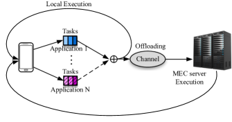
Figure 1: The system model.

In this section, we describe a system architecture consisting of a single MEC server and one mobile device running several applications. We study an age minimization problem and develop the mathematical model for task scheduling and computation offloading.

II-A System Architecture

We consider a status monitoring and control MEC system consisting of a single MEC server and one mobile device as shown in Fig. 1. The mobile device runs $N$ applications to monitor several physical phenomena. A computation task is generated by application only when a change of status occurs. The status information embedded in the updates can be obtained by processing the tasks. Given a set of tasks for each application, this paper focuses on the task scheduling and computation offloading strategy under energy consumption constraints.

II-B Mathematical Modeling

We denote $\mathcal{N}=\{1,2,\ldots,N\}$ as the set of applications with $N=|\mathcal{N}|$ as the total number of applications. We denote $\mathcal{K}_{n}=\{1,2,\ldots,K_{n}\}$ as the set of tasks of application $n$ with $K_{n}=|\mathcal{K}_{n}|$ as the total number of tasks in each application. We consider a time slotted system and the time slot length is $\tau$. We denote $T$ as the total number of time slots. We employ a centralized control architecture, where the MEC server will select one task in each time slot and further partition the data for local computing and computation offloading to the MEC server.

1) Task Scheduling Constraints: We denote $u_{nk}(t)$ as a binary variable to indicate whether or not task $k$ in application $n$ is selected in time slot $t$. When the task is selected, $u_{nk}(t)=1$, otherwise, $u_{nk}(t)=0$. In each time slot, at most one task can be selected to be processed. Then we have:

$$\sum_{n=1}^{N}\sum_{k=1}^{K_{n}}u_{nk}(t)\leq 1.$$ (1)

For task scheduling in each application, the processing order of tasks fulfills the first-come-first-served (FCFS) discipline. Task $k+1$ can be selected until the previous task $k$ is completed. We denote $L_{nk}$ as the data size of task $k$ in application $n$. Denote $L_{nk}(t)$ as the remaining data size of task $k$ in application $n$ at the beginning time slot $t$. Then, when the task is completed, $L_{nk}(t)=0$, otherwise $L_{nk}(t)>0$. We denote ${\mathcal{K}}^{\prime}_{n}$ as the set of tasks of application $n$ except the last task. Then we have:

$$u_{n,k+1}(t)\leq 1-\frac{L_{nk}(t)}{L_{nk}},\quad n\in\mathcal{N},k\in\mathcal{K}^{\prime}_{n}.$$ (2)

If task $k$ in application $n$ is completed, the value of the terms in the right side of inequalities (2) equals to 1, otherwise the value is less than 1.

For task scheduling among different applications, if task $k$ is selected to be processed, consecutive time slots will be allocated to this task until it is completed. After completing this task, time slot will be released for other tasks. When the task is being processed, $0<\frac{L_{nk}(t)}{L_{nk}}<1$, otherwise $\frac{L_{nk}(t)}{L_{nk}}=1$ or $\frac{L_{nk}(t)}{L_{nk}}=0$ . Then we have:

$$u_{nk}(t)\geq(1-\frac{L_{nk}(t)}{L_{nk}})\frac{L_{nk}(t)}{L_{nk}},\quad n\in\mathcal{N},k\in\mathcal{K}_{n}.$$ (3)

If task $k$ in application $n$ is being processed, the value of the terms in the right side of inequalities (3) is a positive number, otherwise the value is 0.

2) Computation Offloading Constraints: In each time slot, the computation offloading strategy will decide the data size processed at mobile device, and the data size offloaded to the MEC server. We denote $D_{loc}(t)$ and $D_{off}(t)$ as the data size processed by local CPU and the MEC server respectively. Obviously, the sum of data size processed in time slot $t$ does not exceed the remaining data size of the selected task. Then we have:

$$D_{loc}(t)+D_{off}(t)\leq\sum_{n=1}^{N}\sum_{k=1}^{K_{n}}u_{nk}(t)L_{nk}(t).$$ (4)

Then at the beginning of next time slot, the remaining data size is

$$L_{nk}(t+1)\!=\!L_{nk}(t)\!-\!u_{nk}(t)(D_{loc}(t)\!+\!D_{off}(t)),n\!\in\!\mathcal{N},k\!\in\!\mathcal{K}_{n}.$$ (5)

3) Energy Consumption Constraints: For local computing, the major energy consumption is the operation of CPU. We denote $\omega$ as the number of CPU cycles required for computing one-bit data at mobile device. For local computing, CPU operation at a constant CPU-cycle frequency is most energy-efficient. We denote $f(t)$ as the CPU frequency of mobile device in time slot $t$. Then, $f(t)$ can be expressed as

$$f(t)=\frac{\omega D_{loc}(t)}{\tau}.$$ (6)

In particular, according to the model in [14], the energy consumption per CPU cycle is proportional to the square of the frequency of CPU. The energy consumption per CPU cycle can be modeled by $E_{cyc}=\gamma f^{2}(t)$, where $\gamma$ is a constant related to chip architecture. Therefore, the energy consumption for local computing can be given by

$$E_{loc}(t)=E_{cyc}\omega D_{loc}(t)=\gamma f^{2}(t)\omega D_{loc}(t)=\alpha(D_{loc}(t))^{3},$$ (7)

where $\alpha=\gamma\omega^{3}/\tau^{2}$.

For computation offloading, the major energy consumption of mobile device includes the energy consumption for task computation offloading, and the energy consumption for downloading the computational results of tasks. We assume that the computational results are relatively small compared to the input data, therefore the energy consumption for downloading the computational results back to the mobile device is neglected.

We denote $h(t)$ as the channel gain between the mobile device and the MEC server in time slot $t$. Denote $P_{off}(t)$ as the transmitted signal power of mobile device. Following the empirical model in [10],[13], the transmitted power consumed by reliable transmitting is a convex monomial function with respect to the achievable data rate. Then the energy consumption for task computation offloading is

$$E_{off}(t)=P_{off}(t)\tau=\lambda_{0}\frac{(D_{off}(t)/\tau)^{m}}{h(t)}\tau=\lambda\frac{(D_{off}(t))^{m}}{h(t)},$$ (8)

where $\lambda=\lambda_{0}/\tau^{m-1}$. $\lambda_{0}$ is the energy coefficient incorporating the efforts of bandwidth and noise power. $m$ is the monomial order determined by the modulation-and-coding scheme and takes on values in the typical range of $2\leq m\leq 5$.

We assume that the energy consumed by the mobile device for processing all tasks does not exceed the upper limit $E_{max}$, then we have:

$$\sum_{t=1}^{T}\{E_{loc}(t)+E_{off}(t)\}\leq E_{max}.$$ (9)

4) AoT Constraints: In real-time monitoring and control applications, users rely on timely situational awareness to make the right decisions. It is important to obtain timely knowledge of the surroundings, to reduce the uncertainty of the system. The sample strategy of this system is sample-at-change, in which the generation of task is event triggered and captures a change of status. The uncertainty of knowledge about the surroundings appears when a new task is generated, and becomes more severe over time if the task is not processed. When the task is completed, the corresponding knowledge of the specific time interval is revealed by the computation results, and the uncertainty of knowledge about the surroundings is reduced to the generation time of the first unprocessed task left in the queue. When all tasks have been processed, the uncertainty of knowledge about the surroundings becomes zero.

We employ the concept of AoT to evaluate the temporal value of computation tasks that can be revealed through the computation of a task. Numerically, AoT is the time elapsed since the first unprocessed task left in the queue is generated. Fig. 2 shows the evolution of AoT in application $n$. For each application, AoT increases by one per time slot if no task is completed. AoT drops to a smaller value when a task of this application is completed. AoT is reset to zero after all tasks of the application are completed.

As shown in Fig. 2, we denote $\tau_{0}$ as the start time of the task scheduling and $a_{n0}$ as the initial age of application $n$. We assume that task $k$ in application $n$ is generated at time $\tau_{nk}$ and completed at time $\tau^{\prime}_{nk}$. The initial AoT of application $n$ is the time interval between start time of the task scheduling and generation time of the first task, $a_{n0}=\tau_{0}-\tau_{n1}$. Denote $a_{n}(t)$ as the instantaneous AoT of application $n$ at time slot $t$. It represents the elapsed time since the first unprocessed task left in the queue is generated. Then $a_{n}(t)$ can be calculated as follows:

$$a_{n}(t)=\begin{cases}a_{n}(t-1)+1,\ \ \;\text{if no task in application $n$ is }\\ \qquad\qquad\qquad\quad\text{completed in time slot $(t-1)$,}\\ t-\tau_{n,k+1},\qquad\ \text{if task $k$ in application $n$ is}\\ \qquad\qquad\qquad\quad\text{completed in time slot $(t-1)$.}\\ \qquad 0,\qquad\qquad\text{if all tasks in application $n$ are }\\ \qquad\qquad\qquad\quad\text{completed.}\end{cases}$$ (10)

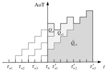
Figure 2: Evolution of AoT in application $n$. The task $k$ in application $n$ is generated at time $\tau_{nk}$ and completed at time $\tau^{\prime}_{nk}$.

Let $A_{n}$ denotes the overall AoT of application $n$. The overall AoT is the area under the finite-length sawtooth ladderlike function in Fig.2, and equals to

$$A_{n}=\sum_{t=1}^{\tau^{\prime}_{n,K_{n}}-\tau_{0}}a_{n}(t),\quad n\in\mathcal{N}.$$ (11)

As shown in Fig. 2, the area under this curve can be decomposed into a sum of disjoint geometric parts. The area can be seen as the concatenation of the parallelogram-like area $Q_{nk}$ for $1\leq\!k\!\leq K_{n}\!-\!1$ and trapezoid-like area $\tilde{Q}_{n,K_{n}}$. This decomposition yields

$$A_{n}=\tilde{Q}_{n,K_{n}}+\sum_{k=1}^{K_{n}-1}Q_{nk},\quad n\in\mathcal{N}.$$ (12)

We denote $\Delta_{nk}$ as the elapsed time between the generation of tasks $k+1$ and $k$ in application $n$. It follows that

$$\Delta_{nk}=\tau_{n,k+1}-\tau_{nk},\quad k\in\mathcal{K}_{n}^{{}^{\prime}}$$ (13)

Then the parallelogram-like area $Q_{nk}$ is:

$$Q_{nk}=\Delta_{nk}(\tau^{\prime}_{nk}-\tau_{0}),\quad n\in\mathcal{N},k\in\mathcal{K}_{n}^{{}^{\prime}},$$ (14)

The trapezoid-like area $\tilde{Q}_{n,K_{n}}$ is:

$$\begin{split}\tilde{Q}_{n,K_{n}}&=(\tau_{0}-\tau_{n,K_{n}})+(\tau_{0}-\tau_{n,K_{n}}+1)+\ldots+\\ &(\tau_{0}-\tau_{n,K_{n}}+\tau^{\prime}_{n,K_{n}}-\tau_{0}-1)\\ &=\frac{(\tau^{\prime}_{n,K_{n}}-\tau_{0})(\tau_{0}-2\tau_{n,K_{n}}+\tau^{\prime}_{n,K_{n}}-1)}{2},\quad n\in\mathcal{N},\end{split}$$ (15)

Therefore, the overall AoT of application $n$ can be calculated as follows:

$$\begin{split}A_{n}=&\frac{(\tau^{\prime}_{n,K_{n}}-\tau_{0})^{2}}{2}+(\tau_{0}-\tau_{n,K_{n}}-\frac{1}{2})(\tau^{\prime}_{n,K_{n}}-\tau_{0})+\\ &\sum_{k=1}^{K_{n}-1}\Delta_{nk}(\tau^{\prime}_{nk}-\tau_{0}),\quad n\in\mathcal{N}.\end{split}$$ (16)

II-C Problem Formulation

To ensure the timely situational awareness about the surroundings, we aim to minimize the sum AoT of all applications under energy consumption constraints. The problem can be formulated as follows:

(P1) $$\min_{u_{nk}(t),D_{loc}(t),D_{off}(t)}\ \sum_{n=1}^{N}A_{n}$$

s.t. $$\textrm{Task scheduling constraints: }\eqref{eq:scheduling 1}-\eqref{eq:scheduling 3};$$

$$\textrm{Computation offloading constraints: }\eqref{eq:Dnk(t)},\eqref{eq:task_length};$$

$$\textrm{Energy consumption constraints:}\eqref{eq:Energy_loc}-\eqref{eq:Energy_sum}$$

$$\textrm{AoT constraints: }\eqref{eq:overall age 1},\eqref{eq:Delta},\eqref{eq:overall age}.$$

In this formulation, $D_{loc}(t)$ and $D_{off}(t)$ are integer variables. $u_{nk}(t)$ is binary variable. $N$, $K_{n}$, $L_{nk}$, $\tau_{nk}$, $h(t)$ are constants. The formulated problem is an INLP, which is intractable. To remove the nonlinear terms in constraint (7) and (8), we employ the piecewise linear approximation technique. Then the problem is transformed into an integer linear program, which can be solved by a commercial solver such as Gurobi [15].

Algorithm 1 An efficient task scheduling algorithm

1:  $empty(n)\!\leftarrow\!0$, $num(n)\!\leftarrow\!1,order\!\leftarrow\!\emptyset,i\!\leftarrow\!1,n\!\in\!\mathcal{N}$

2:  while $sum(empty)\leq N-1$ do

3:     for $n\in\mathcal{N}$ do

4:        Compute $\delta_{n}$

5:     end for

6:     $c\leftarrow argmax(\delta_{n})$, $order(i)\leftarrow c$, $i\leftarrow i+1$, $E(i)\leftarrow E_{c,num(c)}$

7:     Perform task computation offloading, update AoT of each application.

8:     $E(i)\leftarrow E^{\prime}_{c,num(c)}$

9:     if $num(c)\leq K_{n}-1$ then

10:        $num(c)\leftarrow num(c)+1$

11:     else

12:        $empty(c)\leftarrow 1$

13:     end if

14:  end while

15:  for $j=1\ to\ \sum_{n=1}^{N}K_{n}$ do

16:     $E(j)=E_{max}-sum(E)+E(j)$

17:     $empty(n)\leftarrow 0$, $num(n)\leftarrow 1,i\leftarrow 1,n\in\mathcal{N}$

18:     while $sum(empty)\leq N-1$ do

19:        $c\leftarrow order(i),E_{c,num(c)}\leftarrow E(i)$, $i\leftarrow i+1$

20:        repeat lines 7 - 13

21:     end while

22:  end for

III An Efficient Solution

In this section, we present a light-weight age-based task scheduling and computation offloading algorithm. The basic idea is as follows. For task scheduling, we should select the task which reveals the most knowledge about the surroundings and least waiting time for other tasks. For computation offloading, we should decide the data size processed in each time slot as well as the exact portions for local computing and computation offloading to minimize the processing time of the selected task under energy constraints.

For task scheduling, if a task in application $n$ is selected for processing, the change of sum AoT of all applications consists of two parts: 1) the age reduction of application $n$ caused by completing the task, 2) the age increment of applications caused by waiting for the processing of the task. We denote $\delta_{n}$ as the change of the sum AoT of all applications after completing a task in application $n$. Denote $\delta_{n}^{r}$ as the age reduction by completing the task and $\delta_{n}^{i}$ as the age increment due to waiting for the processing of the task, then we have $\delta_{n}=\delta_{n}^{r}-\delta_{n}^{i}$.

First, we look into the details of age reduction caused by completing task $k$ in application $n$. For the set of tasks except the last task, $\delta_{n}^{r}$ equals to $\Delta_{nk}$, which is a constant determined by the task generation interval times defined in constraint (13). For the last task, $\delta_{n}^{r}$ equals to $a_{n}(\tau^{\prime}_{n,K_{n}}-\tau_{0})+1$ because AoT is reset to zero after complete this task, where $a_{n}(\tau^{\prime}_{n,K_{n}}-\tau_{0})$ is the AoT of application $n$ at time slot $\tau^{\prime}_{n,K_{n}}-\tau_{0}$. Then, we consider the age increment of applications. We denote $N^{\prime}$ as the number of applications that have unprocessed task and $s_{nk}$ as the number of time slots needed to process task $k$ in application $n$. Then the total age increment caused by waiting for the processing of task $n$ in application $n$ is $s_{nk}N^{\prime}$.

For computation offloading, we aim at finding the optimal data size for local computing and offloading to minimize the processing time under energy constraints. We denote $E_{nk}$ as the energy assigned to task $k$ in application $n$. We assign an initial energy to each task, which is proportional to the cube of the task length. Then we have:

$$E_{nk}=\frac{(L_{nk})^{3}}{\sum_{n=1}^{N}\sum_{k=1}^{K_{n}}(L_{nk})^{3}}E_{max}.$$ (17)

We denoet $t^{s}_{nk}$ as the time when task $k$ in application $n$ starts to be processed. The computation offloading problem is formulated as follows:

(P2) $$\min_{D_{loc}(t),D_{off}(t)}\ s_{nk}$$

s.t. $$\eqref{eq:Energy_loc},\eqref{eq:Energy_off},$$

$$\sum_{t=t^{s}_{nk}}^{t^{s}_{nk}+s_{nk}}\{D_{loc}(t)+D_{off}(t)\}=L_{nk},$$

$$\sum_{t=t^{s}_{nk}}^{t^{s}_{nk}+s_{nk}}\{E_{loc}(t)+E_{off}(t)\}\leq E_{nk}.$$

The computation offloading problem includes two parts: How many bits can be processed in each time slot? Within each time slot, how many bits should be processed locally and offloaded to MEC server, respectively? If the data size can be processed in time slot $t$ is fixed, we aim to find an offloading scheme to minimize the energy consumption based on channel condition. We denote $D(t)$ as the data size processed in time slot $t$. The energy consumption in a single time slot is

$$E(t)=\alpha(D_{loc}(t))^{3}+\lambda\frac{(D(t)-D_{loc}(t))^{m}}{h(t)}.$$ (18)

Notably, Equation (18) is a convex function. We set the monomial order $m$ as 3 [13]. Using the Lagrangian method, the optimal data allocation for local execution and MEC server execution, $D_{loc}(t)$ and $D_{off}(t)$, are given by

$$D_{loc}(t)=\frac{D(t)}{1+\sqrt{\frac{\alpha h(t)}{\lambda}}}\ \text{and}\ D_{off}(t)=\frac{D(t)}{1+\sqrt{\frac{\lambda}{\alpha h(t)}}}.$$ (19)

Then the minimum energy consumption for execute $D(t)$ bits data in a single time slot $t$ can be obtained as

$$E(t)=\alpha(D(t))^{3}(1+\sqrt{\frac{\alpha h(t)}{\lambda}})^{-2}.$$ (20)

To obtain the value of $D(t)$, we apply feasibility test to find the minimum number of time slots needed to process a task under energy constraints. We first fix the task completion time as one time slot and $D(t)=L_{nk}$ to calculate the energy needed based on Equation (20). If the obtained energy $E^{\prime}_{nk}$ is smaller than the energy limit ($E_{nk}$), the value of $D(t)$ is feasible. Otherwise, we increase the task completion time by one slot and calculate the date sizes processed in each time slot interactively until the resulting energy consumption meet the energy consumption constraint. Note that the data partition among different time slots can be obtained by using Lagrange method for Equation (20).

$$\frac{D(t_{1})}{D(t_{2})}=\frac{1+\sqrt{\frac{\alpha h(t_{1})}{\lambda}}}{1+\sqrt{\frac{\alpha h(t_{2})}{\lambda}}}.$$ (21)

After determining the processing order of tasks, if there is energy left, we assign the rest energy to previous tasks to further reduce the age increment caused by task waiting.

IV Performance Evaluation

In this section, we present simulation results to first answer the following question: Is there a difference between age-based task scheduling and traditional delay-based task scheduling? Moreover, we evaluate the performance of our proposed algorithm and compare the performance between age-optimal strategy and delay-optimal strategy. As for delay-optimal strategy, the completion time of all tasks is minimized. As a performance benchmark, we also simulate the MEC-only strategy where each task is offloaded to MEC server for computing using round-robin task scheduling. Note that the optimal solutions in these three strategies are obtained using a commercial solver Gurobi.

We show that age-optimal strategy outperforms delay-optimal strategy in minimizing the sum AoT of all applications, while it also offers competitive solution in minimizing completion time of all tasks when compared with delay-optimal strategy. We also notice that the MEC-only strategy offers poor performance in terms of both sum age and completion time of tasks. This shows that judicious design of task scheduling and computation offloading strategy is critical.

IV-A Simulation Settings

We consider the mobile device runs 3 applications and each application has 3 tasks that are randomly generated. The time stamp of each task follows the uniform distribution with $[1,8]$. The starting time of the scheduling horizon is $\tau_{0}=10$. The length of time slot is set as 10 ms. The data size of each task follows the uniform distribution with $[400,600]$ (bits). For local computing, the effective energy coefficient of the CPU at mobile device is set as $\gamma=10^{-28}$. Computing one-bit data at mobile device require $\omega=10^{5}$ CPU cycles. For MEC computation offloading, the channel gain in each time slot follows the uniform distribution with $[10^{-5},10^{-3}]$. The energy coefficient and the monomial order are set as $\lambda_{0}=10^{-17}$ and $m=3$, respectively. For each comparison study, we generate 50 random instances and take the average from the results.

IV-B Results

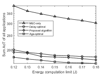
Figure 3: Sum AoT of all applications when energy consumption limit increases from 0.12 (J) to 0.18 (J).

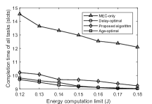
Figure 4: Completion time of all tasks when energy consumption limit increases from 0.12 (J) to 0.18 (J).

We first compare the achievable sum AoT of all applications obtained by the four strategies for different energy consumption limits. Fig. 3 shows the trend of sum AoT of all applications as the energy consumption limit increases from 0.12 J to 0.18 J. Each point on the curve is averaged over results from 50 randomly generated instances. As shown in Fig. 3, the objective values obtained by the four strategies decrease as the energy consumption limit increases, as expected. It shows that (i) MEC-only strategy yields the worst performance; (ii) the age-optimal strategy and the proposed algorithm outperform the delay-optimal strategy (with an average gap of 18.2 slots and 5.7 slots, respectively); (iii) the average ratio between the objective values obtained by the proposed algorithm and those from Gurobi is 93.2%.

We also compare the completion time of all tasks obtained by the four strategies for different energy consumption limits. Fig. 4 shows the trend of completion time of all tasks as the energy consumption limit increases from 0.12 J to 0.18 J. Each point on the curve is averaged over results from 50 randomly generated instances. As shown in Fig. 4, the completion time needed by the four strategies decreases as the energy consumption limit increases, as expected. It shows that (i) MEC-only strategy yields the worst performance; (ii) the performance of both age-optimal strategy and the proposed algorithm are competitive when compared with the delay-optimal strategy (with an average gap of 0.07 slots and 0.43 slots, respectively); (iii) the average ratio between the objective values obtained by the proposed algorithm and those by delay-optimal strategy is 95.6%.

V Conclusions

The emerging real-time monitoring and control applications require timely situational awareness. Therefore, evaluating the temporal value of computation tasks is urgently needed when designing task scheduling strategy. In this paper, we employed the concept of AoT to evaluate the temporal value of information. We studied an age minimization problem in a MEC system consisting of a single MEC server and one mobile device running several applications. The problem formulation involves task scheduling constraints, computation offloading constraints, energy consumption constraints, and falls in the form of an INLP. To solve the problem efficiently, we proposed a light-weight task scheduling and computation offloading algorithm. Simulation results showed that the performance of our proposed age-based scheduling strategy is competitive when compared with traditional strategies.

- [1] P. Mach and Z. Becvar, “Mobile edge computing: A survey on architecture and computation offloading,” IEEE Commun. Surveys Tuts., vol. 19, pp. 1628–1656, Mar 2017.
- [2] Y. Mao, C. You, J. Zhang, K. Huang, and K. B. Letaief, “A survey on mobile edge computing: The communication perspective,” IEEE Commun. Surveys Tuts., vol. 19, pp. 2322–2358, Aug. 2017.
- [3] Y. Kao, B. Krishnamachari, M. Ra, and F. Bai, “Hermes: Latency optimal task assignment for resource-constrained mobile computing,” IEEE Trans. Mobile Comput., vol. 16, pp. 3056–3069, Nov. 2017.
- [4] G. Zhang, W. Zhang, Y. Cao, D. Li, and L. Wang, “Energy-delay tradeoff for dynamic offloading in mobile-edge computing system with energy harvesting devices,” IEEE Trans. Ind. Informat., vol. 14, pp. 4642–4655, Oct. 2018.
- [5] S. Kaul, R. Yates, and M. Gruteser, “Real-time status: How often should one update?,” in Proc. IEEE INFOCOM, pp. 2731–2735, Orlando, USA, March 2012.
- [6] Y. Sun, E. Uysal-Biyikoglu, R. Yates, C. E. Koksal, and N. B. Shroff, “Update or wait: How to keep your data fresh,” in Proc. IEEE INFOCOM, pp. 1–9, San Francisco, USA, April 2016.
- [7] Q. He, D. Yuan, and A. Ephremides, “Optimal link scheduling for age minimization in wireless systems,” IEEE Trans. Inf. Theory, vol. 64, pp. 5381–5394, July 2018.
- [8] Y. Sun, Y. Polyanskiy, and E. Uysal-Biyikoglu, “Remote estimation of the wiener process over a channel with random delay,” in Proc. IEEE ISIT, pp. 321–325, Aachen, Germany, June 2017.
- [9] C. Kam, S. Kompella, G. D. Nguyen, J. E. Wieselthier, and A. Ephremides, “Towards an effective age of information: Remote estimation of a markov source,” in Proc. IEEE INFOCOM, pp. 367–372, Honolulu, USA, April 2018.
- [10] W. Zhang, Y. Wen, K. Guan, D. Kilper, H. Luo, and D. O. Wu, “Energy-optimal mobile cloud computing under stochastic wireless channel,” IEEE Trans. Wireless Commun., vol. 12, pp. 4569–4581, Sep. 2013.
- [11] T. Zhao, S. Zhou, X. Guo, and Z. Niu, “Tasks scheduling and resource allocation in heterogeneous cloud for delay-bounded mobile edge computing,” in Proc. IEEE ICC, pp. 1–7, Paris, France, May 2017.
- [12] Y. Mao, J. Zhang, S. H. Song, and K. B. Letaief, “Stochastic joint radio and computational resource management for multi-user mobile-edge computing systems,” IEEE Trans. Wireless Commun., vol. 16, pp. 5994–6009, Sep. 2017.
- [13] Y. Tao, C. You, P. Zhang, and K. Huang, “Stochastic control of computation offloading to a helper with a dynamically loaded cpu,” IEEE Trans. Wireless Commun., to be published, doi: 10.1109/TWC.2018.2890653
- [14] A. P. Chandrakasan, S. Sheng, and R. W. Brodersen, “Low-power cmos digital design,” IEICE Trans. Electron., vol. 75, no. 4, pp. 371–382, April 1992.
- [15] Gurobi Optimization, LLC, [Online], http://www.gurobi.com.